observed structure of the mean planetary-scale extratropical

circulation

1. surface energy balance disparities2. mean sea-level structure3. mean structure aloft4. baroclinic variability5. the movement of synoptic-scale systems

The images shown herein are based on NCEP/NCAR reanalysis dataset,

accessed thru the Climate Diagnostics Center website,

http://www.cdc.noaa.gov/cgi-bin/DataMenus.pl?dataset=NCEP

We aim to answer these questions:

1. What explains the observed climatological SLP (sea level pressure) distribution and its seasonal variation?

2. What explains the “upper-level” height and flow pattern?

3. How does the upper-level structure relate to the surface lows and highs?

4. How do upper-level trofs move in the baroclinic storm track?

suggested further reading

• Holton Chapter 6.1• Bluestein 1993, esp.

– section 1.1.8 [Climatology of cyclogenesis and anticyclogenesis]– section 1.2.5 [Climatology of lows and highs]

• Palmen and Newton (1969) – various chapters are useful. The book is somewhat outdated, but it is

very legible. • Peixoto and Oort (1992)

– 4.1 transient and stationary eddies– 7.2 mean temperature structure– 7.3 mean height structure– 7.4 mean atmospheric circulation

• An introductory, descriptive overview of the atmospheric general circulation (Word file), if you are not familiar with this.

1. background basics: the Earth’s energy budget (global, annual mean)

-30 +30 net radiation

the units are in % of the TOA incoming solar radiation, i.e. S/4 (S=solar constant = 1380 W/m2)

R = Sn+ Lnand

R H + LE

R = 51 –21 = 30

R = 7 + 23 = 30

surface energy terms:R : net radiationSn: net solar radiation

Ln : net terr. radiationH: sensible heat fluxLE: latent heat flux

the net solar radiation varies considerably with latitude and season

En = Sn + Ln -H-LE

net surface energy flux En

Source: Trenberth and Caron 2001: Estimates of Meridional Atmosphere and Ocean Heat Transports. Journal of Climate, 14, 3433–3443

note: the green-shaded area should equal the orange one. This is true since the area of the green latitudes is far larger than it appears.

zonal mean

note the linear scale

net incoming solar radiation

Snnet outgoing

terrestrial radiation (-Ln)

proportional to Earth surface area

En

The required total heat transport in order to maintain an annual-mean steady state (RT), and estimates of the total atmospheric transport AT from NCEP and ECMWF re-analyses

What about the shortfall??

Seasonal variation of the zonal mean of the meridional heat transport by the atmosphere

PW: petawatt or 1015 W

Source: Trenberth and Caron 2001: Estimates of Meridional Atmosphere and Ocean Heat Transports. Journal of Climate, 14, 3433–3443

answer: that heat is transported by oceans

zonal annual mean ocean heat transports

solid: mean; dashed: ±1 (standard deviation)

Source: Trenberth and Caron 2001: Estimates of Meridional Atmosphere and Ocean Heat Transports. Journal of Climate, 14, 3433–3443

0 +30-30

latitude

The poleward energy transfer that is needed to offset the pole-to-equator net radiation imbalance is accomplished partly by the troposphere, partly by the oceans.

(ºN)

annual mean,northern hemisphere

this graph seems to overestimate the heat transport by oceans (Source: Ackerman and Knox 2003)

seasonal march of Sn, Ln and R

notice how - the latitudinal variation of Sn is far larger than that of Ln and dominates that of R- the zonal asymmetry of R (land-sea contrast) is rather small- the desert areas over land are radiatively deficient (anomalously low R for their latitude, on account of the large Ln loss)

seasonal march of surface energy fluxes

Note how LE and H vary tremendously with season, between land and ocean, and even over land and over ocean. H and LE tend to compensate each other. Their variation can be explained in terms of forested regions vs deserts, warm vs cold ocean currents, the sea ice edge, continental airmasses advected over water, etc. Note that oceans absorb and release far more heat than land (“storage change”)

seasonal march of surface air temperature

note that the amplitude of the annual temperature range is higher at:- higher latitudes- over land rather than over water [this does NOT occur in terms of net radiation Rn]- over large land masses, especially their eastern side

2. Structure of SLP, winds, temperatureseasonal march of sea level pressure and sfc winds

observations:- A see-saw SLP variation dominates over the northern continents, with highs in winter and lows in summer. The seasonal variation of the polar lows and subtropical highs over the northern oceans is also large, and is in opposition to SLP variations over land at corresponding latitudes.- The southern hemisphere is far more zonally symmetric.- Note the extremely low SLP around the Antarctic ice dome.

northern oceans:- polar lows: Aleutian, Icelandic- subtropical highs: Pacific, Bermuda

northern continents: - winter highs: Siberian, Intramtn - summer lows: Pakistan, Sonoran

southern oceans: - circumpolar (southern) low - subtropical highs (3 oceans)

polar perspective

• the following plots are all polar stereographic• the images based on NCEP/NCAR re-analysis dataset, accessed thru

the Climate Diagnostics Center website• either winter or summer is shown, either the northern hemisphere

(NH or the southern (SH)• some maps display ‘zonal anomalies’, i.e. the departures from the

zonal (constant latitude) mean

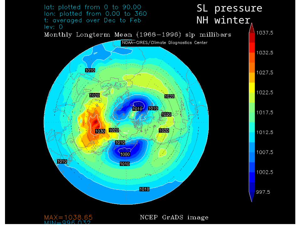
SL pressureNH winter

1000 mb heightNH winter

What SLP is that?Z1000 = 280 m

answer: 280 m ~1035 mb

1000 mb temperatureNH winter

1000 mb temperature, NH winter departure from zonal mean

keep the magnitude of the zonal anomalies in mind

hydrostatic balance implies

• negative surface temperature anomaly high SLP• positive surface temperature anomaly low SLP

• Proof this assuming a flat pressure surface above the cold (warm) anomaly. The depth of this anomaly typically is ~ 2km.

800 mb

ground(sea level)1000 mb

warm Z1000-850 large cold Z1000-850 small

low high

heig

ht

guess when1000 mb height

1000 mb temperature, NH summerdeparture from zonal mean

keep the magnitude of the zonal anomalies in mind

guess when1000 mb height, SH

note how the zonally rather symmetric subtropical high is interrupted over land

1000 mb temperature, SH summerdeparture from zonal mean

note the subtropical warm pools over land, coincident with a low SLP anomaly

note the unusually low SSTs in the eastern subtropical ocean

basins

guess when1000 mb height, SH

1000 mb height, SH winter!

400 m ~1050 mb

1000 mb height, SHAntarctic high removed

ignored

1000 mb temperatureSH winter

1000 mb temperature, SH winterdeparture from zonal mean

ignored

note that these zonal anomalies are relatively small

3. upper-level climatological structure

• focus on winter in the northern hemisphere (NH)

seasonal march of the 500 mb height

wind speed

500 mb heightNH winter

note the seasonal-mean trofs, coincident with the cold anomalies at low levels

1000 hPa temperature

500 mb height (zonal anomaly)NH winter

two quasi-stationary trofs wavenumber 2 pattern

Temperature 850 mb, NH winter

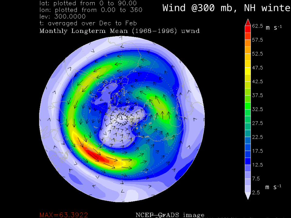
Wind @300 mb, NH winter

m s-1

m s-1

Verify qualitatively that climatological fields are roughly in thermal wind balance. For instance, look at the meridional variation of temperature with height (in Jan)

Around 30-45 ºN, temperature drops northward, therefore westerly winds increase in strength with height

The meridional temperature gradient is large between 30-50ºN and 1000-300 mb

thermal wind

Therefore the zonal windincreases rapidly from 1000 mb up to 300 mb

Question:

Why, if it is colder at higher latitude, doesn’t the wind continue to get stronger with altitude ?

There is definitively a jet ...

Answer: above 300 mb, it is no longer colder at higher latitudes...

tropopause

Tp

Tp

Tropopause pressure (hPa), NH winter

Wind 300 mb, NH winter

80 W

Zonal-mean wind, 80ºW, troposphere and lower stratosphere

Wind @300 hPa, NH winter

A

B

section A, Japantemperature

Japan

tropopause

Japansection A, Japanzonal wind speed

the polar-front jet (PFJ) has merged with the subtropical

jet (STJ)

section B, West Coasttemperature

West Coast of N America

West Coast of N America section B, West Coastzonal wind speed

STJPFJ

Wind 300 mb, NH winter

STJ

PFJ

STJ

PFJ

note that at most longitudes (esp. Asia and the Pacific), a

single jet is present

GP height @ 300 mb, NH winter

Potential vorticity @345 K

stra

tosp

heri

c ai

rtr

opo-

sphe

ric

air

pgPV

Schematic zonal-mean cross section (after Palmen & Newton)

ITCZ

The Palmen-Newton model has three meridional circulation cells in each hemisphere

Note that the three-cell pattern ignores seasonal variation and land-sea contrast.

500 mb omega

note that blue is upward motion (<0)note the rising motion near the ITCZ and subtropical sinking, the latter mainly in the winter hemispherenote the seasonal march of the ITCZ (monsoon)note the rising motion in the baroclinic storm tracknote the sinking (rising) on the lee (upwind) side of mountain ranges

How strong are the meridional cells? (zonal mean)

NH winter

NH summer

Jan

July

HadleyFerrel

NHHadley

FerrelSH

Hadley

note the broad belt of subsidence (12-52ºN) in winter and the broad belt of ITCZ ascent (0-30ºN) in summer.

In the NH winter, over continents, the northern Hadley cell rising branch crosses the Equator into the SH ITCZ,

and its sinking branch extends between 12-50ºN

Effectively ascent dominates in the summer hemisphere, and sinking in the winter hemisphere, and the Hadley cell that straddles the equator is the strongest.

ITCZ

ITCZ

ageostrophic flow & secondary circulation near jet streak

Does this synoptic pattern apply to the mean circulation?

Wind 300 hPa, NH winter

A

B

look for evidence of a secon-dary meridional circulation around the Japan jet streak

Circulation, Section A

ag fvvvffvx

Zg

Dt

Du

)(

x Jet stream

Specific humidity, Section A

Thermally direct!

Precipitation rate

ITCZ

Jet core

Note: the vertical velocity field in jet cores will be revisited later for synoptic jets.

4. SLP and 500 m height intraseasonal variability, as a measure of the frequency of storms due to baroclinic

instability*(the midlatitude ‘storm track’)

a 3-10 day bandpass filter is used to highlight ‘synoptic’ disturbances.

*In theory this may include tropical cyclones, but they are rare

hPa

SLP variability (3-10 day)

mm

hPa hPa

Northern hemisphere storm track, SLP, winter

Northern hemisphere storm track, 500 mb, summerNorthern hemisphere storm track, 500 mb, winter

Northern hemisphere storm track, SLP, summer

hPa

Southern hemisphere storm track, SLP, winter

hPa

Southern hemisphere storm track, SLP, summer

summary: 3-10 day variability

• there is a ‘baroclinic storm’ track between 40-60º latitude

• storms appear vertically coupled – 1000 mb variability similar to 500 mb variability

• storm track intensity (synoptic SLP variability) relates to meridional T gradient– stronger in winter than in summer– strongest east of the continents

• storm track intensity also is stronger over ocean than land

• the NH storm track has larger seasonal variability and is less zonally symmetric than the SH storm track

• Lagrangian perspective: where do lows and highs form and decay??

NH baroclinic storm trackcontour: standard deviation of GPHvector: phase propagation vector

1000 mb 500 mb

Winter cyclogenesisWinter cyclolysis

(Bluestein 1993, p 20)

Sea level cyclone formation and decay around North America

Winter anticyclogenesis

Winter anticyclolysis

(Bluestein p. 25)

anticyclone formation and decay around North America

5. On the movement of trofs and ridges

• Rossby waves result from the conservation of vorticity. The restoring force is or, more generally, the meridional gradient of the absolute vorticity. The resulting circulation causes the wave to propagate westward.

c is the Rossby wave propagation speed, u zonal wind, k and l are zonal and meridional wavenumbers

• In short waves, the advection of relative vorticity dominates. The wave propagation speed is slow and they move with the prevailing westerly flow.

• In long waves, the advection of planetary vorticity dominates. Their speed is large and they are generally stationary, or may retrograde.

22 lkuc

cos2

ady

df

gv

gv

• Trofs may be cut-off from the westerly flow and they become stationary at lower latitudes. Cut-off lows may dissipate or they may be ‘kicked back’ into the main current

• The kicker trof needs to approach the cut-off to within ~2000 km (Henry’s rule)

On the movement of trofs and ridges

On the movement of trofs and ridges

• If the max cyclonic shear is on the upstream side of the trof, the trof will tend to move equatorward, and may deepen.

• If the max cyclonic shear is on the downstream side of the trof, the trof will tend to move poleward.

Hovmöller diagrams

red: short-wave trofsblue: stationary long-wave ridge

Winter 02-03

500 mb height (m)

30-40ºN

all longitudes

24 hr average

Alpine lee cyclogenesis

Source: http://www.cdc.noaa.gov/map/clim/glbcir.shtml

Rockies lee cyclogenesis

question: how does the stationary long-wave pattern shown here matches with the 500 mb anomalies from zonal mean, discussed earlier ?

departure of the 24 hr average from the zonal mean

“blocking” flow aloft

• occurs most frequently in spring around 50°N

• results from an anomalous long-wave ridge that blocks the progression of short waves

• Occurs during ‘low-index’ cycles– high index: strong zonal flow– low index: zonal flow weak, meridional flow strong

• 3 types, qualitatively separated– High-over-low block– Omega block– upper-level ridge

upper-level ridgehigh over low block

omega block

conclusions• A seasonally-variable net surface energy imbalance exists, with En>0 at low latitudes and En<0 at high

latitudes.• The atmospheric component of the meridional heat transfer is achieved in part by the meridional

mean circulation (Hadley), but mainly by the mid-latitude eddy circulation associated with the high variability observed on the 3-10 day timescale (baroclinic eddies).

• The Palmen-Newton model of the general circulation of the atmosphere– Highly simplified (seasonal variations/ land-sea contrast are very important) - applies better in the SH– The only strong meridional cell in the zonal mean circulation is the Hadley cell

• The seasonal variation of SLP in the NH is dominated by the land-sea contrast– The annual temperature range over land, esp the eastern end of the land masses, is far larger than that over the

oceans. This is not explained by the annual range of net radiation, which shows weak zonal anomalies.– Subtropical (~30ºN) ocean highs and continental lows dominate in summer– Polar (~60ºN) ocean lows and continental highs dominate in winter

• A jet stream exists in the upper mid-latitude troposphere– Its climatological position and strength are in thermal wind balance, thus it is stronger in winter than in summer– The separation between STJ and PJ is not present at all longitudes, nor in the zonal mean, in both hemispheres &

seasons– Highly zonally asymmetric in the NH, due to continents and topography

• Quasi-stationary trofs along east coasts of N America & Asia• Very symmetric in the SH

– Jet stream separates reservoirs of very different air (in terms of potential vorticity)

• The jet stream carries quasistationary long waves and eastward-moving, baroclinic short waves– baroclinic storm track most apparent in the 3-10 band-pass filtered data, at LL and UL– stronger in winter than summer, – storm track most ‘intense’ near east coasts, where the UL jet and LL baroclinicity are strongest – this is consistent with QG theory (stronger PVA and WAA), to be discussed later

meridional cross section (potential temperature, zonal wind speed)

pre

ssure

(m

b)

latitudeHolton (2004) p.145

W

E

Relationship between surface cyclone and UL wave trof, during the lifecycle of a frontal disturbance

500 mb height (thick lines)SLP isobars (thin lines)

layer-mean temperature (dashed)

The deflection of the upper-level wave contributes to deepening of the surface low.