Empirical Mode Reduction in a Model of Extratropical … · Empirical Mode Reduction in a Model of...

Empirical Mode Reduction in a Model of Extratropical Low-Frequency Variability

D. KONDRASHOV, S. KRAVTSOV, AND M. GHIL*

Department of Atmospheric and Oceanic Sciences, and Institute of Geophysics and Planetary Physics, University of California,Los Angeles, Los Angeles, California

(Manuscript received 16 April 2005, in final form 21 November 2005)

ABSTRACT

This paper constructs and analyzes a reduced nonlinear stochastic model of extratropical low-frequencyvariability. To do so, it applies multilevel quadratic regression to the output of a long simulation of a globalbaroclinic, quasigeostrophic, three-level (QG3) model with topography; the model’s phase space has adimension of O(104).

The reduced model has 45 variables and captures well the non-Gaussian features of the QG3 model’sprobability density function (PDF). In particular, the reduced model’s PDF shares with the QG3 model itsfour anomalously persistent flow patterns, which correspond to opposite phases of the Arctic Oscillationand the North Atlantic Oscillation, as well as the Markov chain of transitions between these regimes. Inaddition, multichannel singular spectrum analysis identifies intraseasonal oscillations with a period of 35–37days and of 20 days in the data generated by both the QG3 model and its low-dimensional analog.

An analytical and numerical study of the reduced model starts with the fixed points and oscillatoryeigenmodes of the model’s deterministic part and uses systematically an increasing noise parameter toconnect these with the behavior of the full, stochastically forced model version. The results of this studypoint to the origin of the QG3 model’s multiple regimes and intraseasonal oscillations and identify theconnections between the two types of behavior.

1. Introduction

We analyze the output of a global, three-level, quasi-geostrophic (QG3) atmospheric model with topogra-phy (Marshall and Molteni 1993; D’Andrea and Vau-tard 2001; Kondrashov et al. 2004). As shown by theseauthors, the QG3 model has a fairly realistic climatol-ogy and rich variability, which also compares favorablywith atmospheric behavior observed in Northern Hemi-sphere (NH) midlatitude flows. In addition to synopticvariability associated with baroclinic eddies, the modelis characterized on longer time scales by the existenceof a few persistent and recurrent flow patterns, orweather regimes (Reinhold and Pierrehumbert 1982;

Legras and Ghil 1985; Molteni 2002), as well as by in-traseasonal oscillations (Ghil and Robertson 2000,2002; Kondrashov et al. 2004).

These coarse-grained features of the model’s low-frequency variability (LFV) may be better understoodby using reduced models, which have considerablyfewer degrees of freedom. Such models can accuratelyrepresent both linear and nonlinear aspects of the fullmodel’s LFV, while parameterizing the effect of higher-frequency, synoptic transients on LFV (Robinson 1996,2000; Lorenz and Hartmann 2001, 2003; Kravtsov et al.2003, 2005a). In this paper, we construct and analyzesuch a reduced nonlinear model, which is based solelyon the output of a long QG3 simulation and involves astochastic parameterization of the synoptic eddies’ ef-fect on the full model’s LFV (Kravtsov et al. 2005b).

To construct reduced dynamical models, one oftenrewrites the full dynamical model equations in terms ofempirical orthogonal functions (EOFs; Preisendorfer1988) derived from a long simulation of the latter. Theequations in this basis are then truncated by retainingonly a few leading EOFs that represent large-scale,low-frequency flow (Rinne and Karhila 1975; Schubert1985; Sirovich and Rodriguez 1987; Mundt and Hart

* Additional affiliation: Département Terre-Atmosphère-Océan, and Laboratoire de Météorologie Dynamique du CNRS/IPSL, Ecole Normale Supérieure, Paris, France.

Corresponding author address: Dr. Dmitri Kondrashov, Dept.of Atmospheric and Oceanic Sciences, and Institute of Geophys-ics and Planetary Physics, University of California, Los Angeles,405 Hilgard Ave., Los Angeles, CA 90095-1565.E-mail: [email protected]

JULY 2006 K O N D R A S H O V E T A L . 1859

© 2006 American Meteorological Society

JAS3719

1994; Selten 1995, 1997), while the residual varianceassociated with the remaining EOFs is usually treatedas random forcing. Alternatively, one can develop adeterministic, flow-dependent parameterization ofthese fast unresolved processes based on the library ofdifferences between the tendency of the full and trun-cated models (D’Andrea and Vautard 2001; D’Andrea2002). Yet another approach to this closure problem,which is mathematically rigorous in the limit of signifi-cant scale separation, has been developed by Majda etal. (1999, 2001, 2002, 2003). Franzke et al. (2005) haverecently applied this approach to a barotropic model onthe sphere, with a T21 resolution, while C. Franzke andA. Majda (2005, personal communication) have appliedit to the QG3 model.

The closure problem above can be effectively ad-dressed in a data-driven, rather than model-driven ap-proach, by using inverse stochastic models; these mod-els rely almost entirely on the dataset’s informationcontent, while making only minimal assumptions aboutthe underlying dynamics. The simplest type of inversestochastic model is the so-called linear inverse model(LIM; Penland 1989, 1996; Penland and Ghil 1993), inwhich the dependence of the state vector’s time deriva-tives on the state vector itself is assumed to be linear,while the time-dependent flow is forced by spatiallycorrelated white noise. LIMs have shown some successin predicting El Niño–Southern Oscillation (ENSO;Penland and Sardeshmukh 1995; Johnson et al. 2000),tropical Atlantic sea surface temperature variability(Penland and Matrosova 1998), as well as extratropicalatmospheric variability (Winkler et al. 2001).

Kravtsov et al. (2005b) have recently developed gen-eralizations of LIMs that relax the assumptions ofmodel linearity and of the noise being white in time.Colored noise, in particular red noise, can be accom-modated by allowing additional model levels, whichpermit one to achieve truly white noise at the last level;model nonlinearities are accommodated in the deter-ministic part of the first level. Such nonlinear, multiple-level inverse models have proven useful in modelingLFV of NH geopotential height anomalies (Kravtsov etal. 2005b), as well as tropical sea surface temperaturevariability (Kondrashov et al. 2005). In the present pa-per we apply methodology of Kravtsov et al. (2005b)and of Kondrashov et al. (2005) to obtain reduced ana-logs of the QG3 model. The best reduced model soobtained is then used to shed light on the full model’sLFV.

The paper is organized as follows. In section 2, wedescribe the experimental setup of the QG3 model andthe statistical methods used to analyze its behavior; themultilevel regression modeling technique used to con-

struct the reduced model is reviewed in the appendix.An excellent match between the statistical properties ofthe full and reduced models is documented in section 3,in terms of both intraseasonal oscillations and multipleflow regimes. In section 4 we interpret the results ofsection 3 by examining quasi-stationary states and lin-ear eigenmodes of the deterministic part of the reducedmodel, and study the behavior of this model as a func-tion of the stochastic forcing amplitude. Concluding re-marks follow in section 5.

2. Data and methodology

We analyze the daily output from a perpetual-wintersimulation that is 54 000 days long and was described indetail by Kondrashov et al. (2004). Each of the threelevels of the QG3 model has 1024 grid points in the NH.Since the model’s LFV is equivalent barotropic, we ap-ply principal component (PC) analysis to its NH 500-hPa streamfunction anomalies to reduce the dataset’sdimensionality; in computing EOFs, the anomalies areweighted by the cosine of the latitude (Branstator1987).

We study the QG3 model’s behavior in the phasespace spanned by its leading EOFs by applying twodistinct types of statistical data analysis: probabilitydensity function (PDF) estimation via Gaussian mix-tures (Smyth et al. 1999; Hannachi and O’Neil 2001;Kondrashov et al. 2004) and the multichannel versionof singular spectrum analysis (M-SSA; see Ghil et al.2002 and references therein). These two types of analy-sis correspond to two complementary descriptions ofLFV: (i) the episodic one in terms of anomalously per-sistent multiple flow regimes, and the Markov chain oftransitions between them; and (ii) the one that empha-sizes low-frequency oscillations (Ghil and Robertson2002).

The weather regimes correspond to the k clustersobtained by the Gaussian mixture analysis applied inthe subspace of d leading EOFs. The optimal numberk* of clusters is determined using a built-in criterion,based on cross-validated log-likelihood estimates. Eachdata point has a degree of membership in several clus-ters, depending on its position with respect to each clus-ter centroid and the weight of that cluster. Based on acombination of these two criteria, one can associateeach point with a unique cluster and obtain the com-posite pattern of anomalies associated with this cluster.Furthermore, we define regime events as the number ofconsecutive points (days) along the model trajectorythat fall within a given cluster, and compute variousquantities related to conditional probabilities of regimeoccurrence, which characterize the statistics of the tran-

1860 J O U R N A L O F T H E A T M O S P H E R I C S C I E N C E S VOLUME 63

sitions between regimes (Mo and Ghil 1988; Kimotoand Ghil 1993b). The preferred transition paths soidentified may, in certain cases, be associated with low-frequency oscillations present in the dataset (Ghil et al.1991; Kondrashov et al. 2004).

These oscillations will be identified here by M-SSAanalysis (Keppenne and Ghil 1993), which is especiallyuseful in the study of amplitude- and phase-modulatedsignals. M-SSA finds eigenvalues and eigenvectors ofthe grand covariance matrix built from lagged copies ofa vector time series. An oscillatory mode is character-ized by a pair of nearly equal eigenvalues and periodiceigenvectors that correspond to the same frequency.Following Ghil et al. (2002), we apply a Monte Carlotest to ascertain statistical significance of the oscilla-tions detected by M-SSA. In addition, we subject sus-pected oscillatory pairs to the lag-correlation test ofPlaut and Vautard (1994). All oscillatory signals iden-tified in section 3 pass both of these tests.

The data-adaptively bandpass-filtered time series as-sociated with the oscillatory modes are called recon-structed components (RCs), which we use to define theoscillation’s phase categories (Keppenne and Ghil1993; Plaut and Vautard 1994). Similarly to the regimecompositing described above, we also performed acomposite analysis keyed to a given phase of a low-fre-quency oscillation to describe the anomalies in physicalspace associated with that phase (Ghil and Mo 1991;Plaut and Vautard 1994).

The statistical significance of any composite quantitycan be estimated using a nonparametric Monte Carlomethod (Dole and Gordon 1983; Vautard et al. 1990;Plaut and Vautard 1994). To do so, one gathers intotime segments the consecutive days belonging to agiven oscillation phase or a given regime, including a“null regime,” defined as all data points that do notbelong to any of the regimes identified. These segmentsare randomly shuffled 100 times, thus providing 100independent realizations with the same length as theoriginal time series. Each quantity estimated for a givencomposite, whether keyed to a given regime or to anoscillation’s given phase category, can also be com-puted using the 100 shuffled sets of category numbers.The 95% confidence interval, for example, is thenbounded by the 2.5th and 97.5th percentiles of the ran-dom values so computed, sorted in ascending order.

The procedure for constructing the reduced modelhas been described in detail by Kravtsov et al. (2005b)and is reviewed here briefly in the appendix. The modelhas, in general, I variables at the first level and N levels;see Eq. (A1). We chose the number I of state vectorcomponents (EOFs) to achieve maximal correspon-dence between the behavior of the reduced model and

full QG3 model in terms of their PDF structure and theperiods, as well as spatial patterns, of low-frequencyoscillations in each model. The reduced model with I �15 variables and quadratic nonlinearities at the firstlevel produced optimal results, while the number oflevels is N � 3, and it is given by the requirement thatthe additive noise be truly white at the last level; seeKravtsov et al. (2005b). The total number of variablesin the inverse model is thus I � N � 15 � 3 � 45, twoorders of magnitude less than that in the full QG3model.

3. Weather regimes and intraseasonal oscillations

We performed long simulations (�54 000 days) ofthe reduced model (A1) with I � 15 and N � 3, usinga time step of �t � 1 day. In this section, we comparethe statistical properties of the datasets produced by thereduced model and the full QG3 model.

a. Weather regimes

The PDF of the datasets produced by the QG3 andthe reduced model are shown Fig. 1 in the subspace ofthe QG3 model’s three leading EOFs. The clusterswere found using mixtures of k � 4 Gaussian compo-nents in a phase subspace of three leading EOFs, whichcapture 25% of the total variance. The optimal numberof clusters is k � 4 for both the QG3 simulation and forthe reduced-model dataset, as determined by the cross-validation procedure of Smyth et al. (1999); see alsoKondrashov et al. (2004). The locations, shapes andsizes of clusters, and hence the general shape of theQG3 model’s PDF, are well reproduced by our reducedmodel’s PDF in Fig. 1. On the other hand, linear re-duced models driven by Gaussian noise cannot capturethe clearly non-Gaussian shape of the QG3 model’sPDF and the associated weather regimes; see furtherdiscussion of this point in Kravtsov et al. (2005b) andKondrashov et al. (2005).

The composites over the data points that belong toeach of the ellipses in Fig. 1 represent, in physical space,the patterns of four planetary flow regimes (Legras andGhil 1985; Ghil and Childress 1987, chapter 6; Mo andGhil 1988; Cheng and Wallace 1993; Kimoto and Ghil1993a,b; Hannachi 1997; Smyth et al. 1999; Hannachiand O’Neill 2001; Molteni 2002). These regimes areassociated with the opposite phases of the NH annularmode, the so-called Arctic Oscillation (AO; Deser2000; Thompson and Wallace 2000; Thompson et al.2000; Wallace 2000), and the sectorial North AtlanticOscillation (NAO; Hurrel 1995) pattern.

In Fig. 1a, cluster AO� occupies a distinctive regionon the PDF ridge that stretches along EOF-1. It corre-


sponds to the low-index phase of the AO (Deser 2000;Wallace 2000). The clusters AO�, NAO�, and NAO�

are located around the global PDF maximum, with thecentroid of AO� to the left and below, NAO� above,and NAO� slightly to the right of this maximum, re-spectively. These four regimes are not identical to butin fairly good agreement with the observational resultsof Cheng and Wallace (1993) and Smyth et al. (1999);see also Ghil and Robertson (2002) and Kondrashov etal. (2004).

Since we are ultimately interested in explaining LFVin NH observations, one might question the indepen-

dence of the two NAO-related and the two AO-relatedregimes in the QG3 model. The relations betweenhemispheric and sectorial regimes are a topic of con-tinuing investigation and debate. Watanabe (2004), forinstance, showed, using both NH observations and alinear barotropic model, how the sectorial NAO couldhave, at certain times of year and in combination withother sectorial phenomena, a downstream effect ex-tending all the way to East Asia. Kravtsov et al. (2006),on the other hand, distinguish in NH observations be-tween a more truly hemispheric character of AO� ver-sus more complex and sectorial manifestations of AO�.

FIG. 1. Mixture model PDF and clusters of the four weather regimes—AO�, AO�, NAO�, and NAO� (see text)for the (left) QG3 model and (right) reduced. (a), (b), (c) Projections onto pairs of EOFs, as indicated on the axes.The semiaxes of the ellipses equal the standard deviation (i.e., the eigenvalue) in each principal direction.


As we shall see in section 4, these observational resultsare reflected in the reduced model’s AO� regime beingassociated with a stable fixed point of our model’s de-terministic part.

The streamfunction anomalies associated with eachregime centroid of the QG3 model are plotted in Fig. 2.The spatial correlations between these anomaly pat-terns and those obtained from the reduced model (notshown) all exceed 0.9. They are thus much higher thanthe correlations obtained by D’Andrea and Vautard(2001) and D’Andrea (2002) in their 10-variable re-duced model.

b. Intraseasonal oscillations

We compare the results of M-SSA analysis for theQG3-model and the reduced-model simulations in Fig.3. Both datasets have the same length of 54 000 days.M-SSA was applied to the time series of the three lead-ing PCs of the QG3 data. The QG3-model spectrum(dashed line) and the reduced-model spectrum (solidline) show excellent agreement in terms of overallshape, as well as in the location of the leading signifi-cant oscillatory pair, marked by an arrow. This oscilla-tory mode has a period of about 37 days in both models

FIG. 2. Mixture-model centroids, showing streamfunction anomaly maps at 500 hPa, for the QG3 model: (a)NAO�, (b) NAO�, (c) AO�, and (d) A��. Positive contours are thick and land masses are shaded; 20 contourlevels between maximum and minimum values are used, with the following intervals (in 106 m2 s�1): (a) 1.1, (b) 0.8,(c) 0.8, and (d) 1.1. Reproduced from Kondrashov et al. (2004), with the permission of the American Meteoro-logical Society.


and will be analyzed in detail in the remainder of thispaper. The second, less energetic, oscillatory mode hasa period of about 20 days in the QG3 model (see Kon-drashov et al. 2004), and lies outside of the frequencyrange of Fig. 3. This secondary mode is also present inthe reduced model, but is less robust (see section 4bbelow). The other spectral peaks in Fig. 3 correspond tosingle PCs and not to oscillatory pairs in M-SSA.

The composite maps keyed to the phases of this os-cillation (see section 2) are shown in Fig. 4 for theQG3-model simulation. The reduced model producesresults that are virtually identical to those in Fig. 4 (notshown). Figures 4a–d illustrate four successive, equallypopulated composites that, taken together, cover one-half cycle of the oscillation.

The composites of Figs. 4a,d,b have a strong resem-blance to the NAO�, NAO�, and AO� flow-regimecentroids of Figs. 2a–c, respectively. After passingthrough the NAO� (Fig. 4a) and AO� (Fig. 4b) phases,the next phase of our reduced model’s oscillation re-sembles the Pacific–North American (PNA) pattern(Fig. 4c), before reaching the NAO� phase (Fig. 4d);the PNA is a well-known pattern that, along with theAO and NAO, characterizes dominant modes of theNH LFV (Wallace and Gutzler 1981; Ghil and Robert-son 2002). Overall, this oscillation shares several fea-tures of the oscillatory topographic instability describedby Ghil and associates in a hierarchy of models and inNH observations (Legras and Ghil 1985; Jin and Ghil

1990; Ghil and Mo 1991; Ghil and Robertson 2000; Lottet al. 2001, 2004a, b); see Kondrashov et al. (2004) fora more detailed discussion.

c. Connection between regimes and oscillations

The similarity between the regime composites andcertain phases of the low-frequency oscillations de-scribed in the previous subsection points to possiblerelationships between the episodic and oscillatory de-scriptions of LFV (Ghil et al. 1991; Kimoto and Ghil1993b; Plaut and Vautard 1994; Ghil and Robertson2002; Koo et al. 2002; Kravtsov et al. 2006). Kon-drashov et al. (2004) computed conditional probabili-ties of regime transitions for the QG3 model and iden-tified the preferred cycle NAO� → AO� → NAO�,which is consistent with the trajectory of the intrasea-sonal oscillation. We have computed the transitionprobability matrix for our reduced model (not shown)and have found it to be almost identical to that of theQG3 model (see Kondrashov et al. 2004, their Table 6).

The relationship between the regimes and oscilla-tions can be quantified by computing the conditionalprobability of a given regime occurrence, assuming theknowledge of the intraseasonal oscillation’s phase cat-egory (see section 2), as shown in Fig. 5a for the QG3model (left panel) and the reduced model (right panel).In both models, the NAO�, NAO�, and AO� regimesare associated with the same distinct phases of the in-traseasonal oscillation, while the occurrence probabilityof the AO� regime does not strongly depend on theoscillation’s phase category. This is consistent with theoscillation’s spatial patterns in Fig. 4, of which onlythree resemble one of the four flow regimes. Small dif-ferences in phase categorization between Fig. 4 and Fig.5 are due to the fact that phases of the 37-day oscilla-tion strongly resemble, but are not identical to theweather regimes; compare Figs. 2 and 4.

To examine further the relationship between regimesand oscillations, we computed the composite phase ve-locity in the plane spanned by the pair of RCs thatcaptures most of the variance associated with the in-traseasonal oscillation, and the corresponding ten-dency. This pair is given, in both models, by RCs 8–9.Since the RCs in M-SSA are themselves vector-valuedtime series, we used the second channel, denoted byRC*-2, of this pair, along with its tendency. Both RC*-2and the tendency time series were normalized by theirrespective standard deviations; with this normalization,a purely sinusoidal oscillation has a constant phase ve-locity (see Kravtsov et al. 2006).

The results are shown in Fig. 5b for the QG3-model(left panel) and the reduced model (right panel): forboth models, the trajectory slows down considerably in

FIG. 3. M-SSA of QG3 model (dashed line with squares) andreduced-model (solid line with circles) simulations. M-SSA is per-formed in a subspace spanned by the three leading EOFs of theQG3 model. Symbols show M-SSA eigenvalues, plotted againstthe dominant frequency associated with the corresponding space–time PCs. The arrow indicates a significant oscillatory pair with aperiod of about 37 days; the 20-day pair lies outside the frequencyrange shown.


the AO� and NAO� regimes, while it accelerates in theNAO� regime. These results are consistent with alarger number of days and regime events for the high-index AO� and blocked NAO� regimes, when com-pared to these quantities for the zonal NAO� regime(Kondrashov et al. 2004).

4. Analysis of the reduced model

To identify the roots of multiple flow regimes andintraseasonal oscillations, we study in sections 4a and4b the properties of the full dynamical operator of Eq.(A1) obtained by dropping the stochastic forcing termdr(2) at the third and last level of the reduced model. In

this study, we also consider the even simpler, quadraticoperator obtained by retaining only the deterministiccomponent of the model’s first level. Section 4c thentraces the onset of the complete behavior described insection 3, as the stochastic forcing amplitude changesfrom zero to the value obtained by the inverse model-ing procedure described in section 2 and the appendix.

a. Steady and quasi-stationary states

We identify quasi-stationary states of the reducedmodel’s full dynamical operator by computing multiplelocal minima of the quadratic functional defined as thesum, over all 45 state variables, of their squared ten-dencies (Legras and Ghil 1985; Mukougawa 1988; Vau-

FIG. 4. Phase composites of the 500-hPa streamfunction anomalies associated with the 37-day oscillation in theQG3 model: (a)–(d) One-half of the oscillation cycle, with the same plotting conventions and contour intervals asin Fig. 2. Reproduced from Kondrashov et al. (2004), with the permission of the American Meteorological Society.


tard and Legras 1988). To do so, we apply a “subspacetrust region” technique from Matlab’s OptimizationToolbox. This method is based on the interior-reflec-tive Newton procedure (Coleman and Li 1994, 1996),which involves approximate solutions of the minimiza-tion problem for this functional; these solutions, in turn,rely on using a preconditioned conjugate-gradientmethod. The degree of quasi-stationarity of the mini-mal-tendency states so obtained is controlled by a pre-set tolerance �: for a given � and a given initial guess ofthe solution, the procedure iteratively corrects the so-lution until the value of the functional drops below �.

The values of � we use below should be compared withthe typical variance of the reduced model’s state vector,which is approximately equal to 10�2. Once � is chosen,we repeat the minimization procedure many times forrandomly chosen initial states.

For � � 10�8, the procedure converges to the singlesolution located in the vicinity of the AO� regime (seeFig. 1), irrespective of the initial guess used. This is atrue steady state, which is linearly stable (see section 4bbelow) and can be obtained by direct integration of thereduced-model equations with no stochastic forcing.The AO� regime in the reduced-model and in the full

FIG. 5. Regimes vs oscillations for the (left) QG3-model and the (right) reduced-model simulation: (a) prob-ability of a given regime occurrence during one of the eight phase categories of the 37-day oscillation for NAO�

(circles), AO� (diamonds), NAO� (squares), and AO� (triangles); (b) composite phase velocity of the modeltrajectory keyed to the phase categories of the 37-day oscillation (see text). Dashed lines in all panels correspondto 95% confidence levels based on the nonparameteric Monte Carlo test of Plaut and Vautard (1994).


QG3 model simulations is thus associated with the pres-ence of this stable fixed point in the reduced model’sdynamical operator.

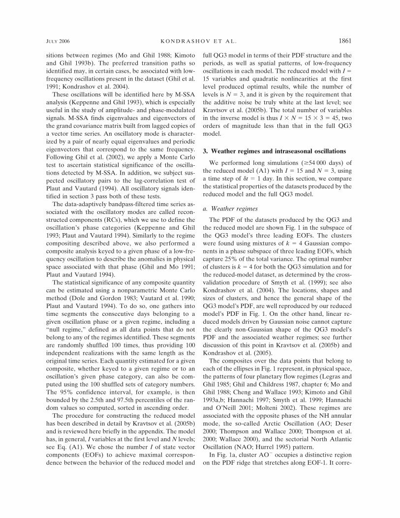
As � increases, we find multiple local minima thatcorrespond to quasi-stationary states of the reducedmodel. The locations of these minima in the phasespace of the latter’s three leading EOFs are shown inFig. 6, for � � 10�6 in Fig. 6a and � � 10�5 in Fig. 6b.If � is sufficiently small, � � 10�7, the quasi-stationarystates are still located mostly in the vicinity of the AO�

regime (not shown). With increasing �, these statesstart to progressively spread out toward the climato-logical mean of the full QG3 model and form a distinct“tongue” (Figs. 6a,b) aligned along the EOF-1 axis.

This small-tendency region in the reduced model’sphase space is thus responsible for the PDF ridge inFigs. 1a,b.

b. Linear stability analysis

We perform here a linear stability analysis of thereduced model’s fixed points. The eigenvectors associ-ated with pairs of complex eigenvalues representdamped oscillations, whose decay time and period arerelated to the inverse of the corresponding eigenvalue’sreal and imaginary parts, respectively.

The dynamical operator we considered so far arisesby dropping the white-noise forcing dr(2) at the thirdlevel; as a result, dr(1) and dr(0) also become determin-

FIG. 6. Quasi-stationary states of the reduced model (open circles) plotted in the phasespace spanned by the QG3 model’s leading EOFs. The degree of quasi-stationarity is presetby selecting a threshold � for the norm of the tendency vector in Eq. (A1) (see text): (a) � �10�6, (b) � � 10�5. Also shown in each panel are the cluster centroids corresponding to thefour weather regimes of the QG3 model in Fig. 1 (filled circles), as well as the trajectory of its37-day oscillatory mode (solid lines and arrows, whose length is scaled according to themagnitude of phase velocity).


istic. It is quite useful to investigate the fixed points ofthe reduced model’s deterministic operator at the firstlevel as well. Instead of a single stable steady state forthe full dynamical operator with all 3 levels discussed insection 4a, two steady states are found: one of them islocated near the AO� regime and it is linearly unstable,with a growth rate of 25 days (see below), while theother is located near the climatology and it is stable.The locations of all fixed points are shown in Fig. 7a,while the eigenspectrum for each of them is shown inFig. 7b.

For the unique steady state of the full, three-leveloperator (diamonds in Figs. 7a,b), all of the eigenmodesare decaying. The two least-damped modes are oscilla-tory; they are characterized by a decay time of approxi-mately 6 days, and have periods of 20 and 35 days,respectively. These two periods are close to the onesobtained by M-SSA analysis of the full QG3 and re-duced-model solutions in section 3b (see also Kon-drashov et al. 2004). It is tempting, therefore, to inter-pret the oscillations identified in the two models’ simu-lations as these damped modes. In the reduced modelthey are excited by the stochastic forcing, while in thefull QG3 model their excitation is due to the smaller-scale modes that have been filtered out of the deter-ministic dynamics by our mode-reduction approach.

The trajectory of the 37-day intraseasonal oscillation,which is shown in Figs. 6a,b, evolves around the time-mean state of the QG3 model, rather than around themodel’s steady state. This result is consistent with thefact that the AO� regime does not appear to be asso-ciated with our 37-day oscillation (see section 3c hereand section 5 in Kondrashov et al. 2004).

We computed therefore the linear eigenmodes of thereduced model linearized about the climatologicalmean state and found that the least-damped eigenmodein this case has a decay time of 6 days and a period of37 days (filled circles in Figs. 7a,b), similar to what weobtained when linearizing about the unique steady stateof the reduced model’s full dynamical operator. The20-day mode, however, is strongly damped when lin-earizing about the reduced model’s climatology, with adecay time of 3 days or less (not shown), which mightexplain the dominance of the 37-day cycle in the QG3model and in NH observations.

A similar separation in periods is observed in theoscillatory modes associated with the fixed points of thefirst-level dynamical operator. The least-damped modefor the unstable steady state near AO� (downward-pointing triangles in Figs. 7a,b) has a decay time of 15days and a period of 25 days, while the correspondingmode for the stable steady state near the climatology(filled squares in Figs. 7a,b) has a period of 35 days and

a decay time of 16 days; note that the instability of theformer steady state is of exponential, rather than oscil-latory type.

The shorter decay times of the oscillatory eigen-modes and the transformation of the steady state nearAO� from unstable to stable, when going from thefirst-level to the three-level deterministic dynamics, in-dicate that the two additional, linear levels involved inmodeling the red-noise forcing levels play a dampingrole. This role makes both mathematical and physicalsense. Mathematically, red noise is associated with lin-ear damping of white noise, which is thus correctly cap-tured by the two additional levels. Physically, the effectof the smaller scales on the large ones can involvepumping energy into the latter, but also damping insta-bilities associated with their self interaction.

Figure 8 shows the real (Fig. 8a) and imaginary (Fig.8b) parts of the 37-day mode obtained by linearizing

FIG. 7. Fixed points of the reduced model and their stability. (a)Fixed points of the reduced model’s deterministic operator:unique, stable steady state for the operator with all three levels(diamond), and linearly unstable (downward-pointing triangle)and stable (filled square) steady states for operator with the firstlevel only; the filled circle denotes the climatological state. (b)Eigenvalues of the reduced model’s deterministic operator linear-ized about the fixed points in (a) and climatology. The two least-damped oscillatory modes for the unique steady state of the op-erator with three levels have periods of 20 and 35 days, and adecay time of 6 days; the corresponding modes of the first-leveldeterministic operator have a period of 35 and 25 days, and decaytimes of 16 and 15 days for the stable and unstable steady state,respectively. The symbols correspond to the fixed points and cli-matology in (a).


the full dynamical operator of the reduced-model equa-tions about climatology, while Figs. 8c,d show the pat-terns for the 35-day mode obtained by linearization ofthe same operator about its unique steady state. Thespatial patterns of these two eigenmodes are remark-ably similar.

The similarity between the two patterns can be inter-preted as follows. Both the AO� regime and the re-duced model’s steady state are primarily associatedwith the weakening and southward shift of the jetstream position, with respect to climatology. Thechanges to the jet stream that are related to the AO�

anomaly have, therefore, a large degree of zonal sym-metry (see Fig. 2d) so that their self-interaction tends to

vanish. This feature is consistent with the presence of atongue of quasi-stationary states along the EOF-1 axisin Fig. 6. The approximate invariance of the least-damped eigenmodes of the reduced-model equations,when linearized about either the climatological jet or itsuniformly shifted counterpart means that the least-damped eigenmodes are not sensitive to AO-typechanges of the basic state. In other words, the eigen-modes turn out to be patterns whose interaction withAO-type changes of the midlatitude jet vanishes.

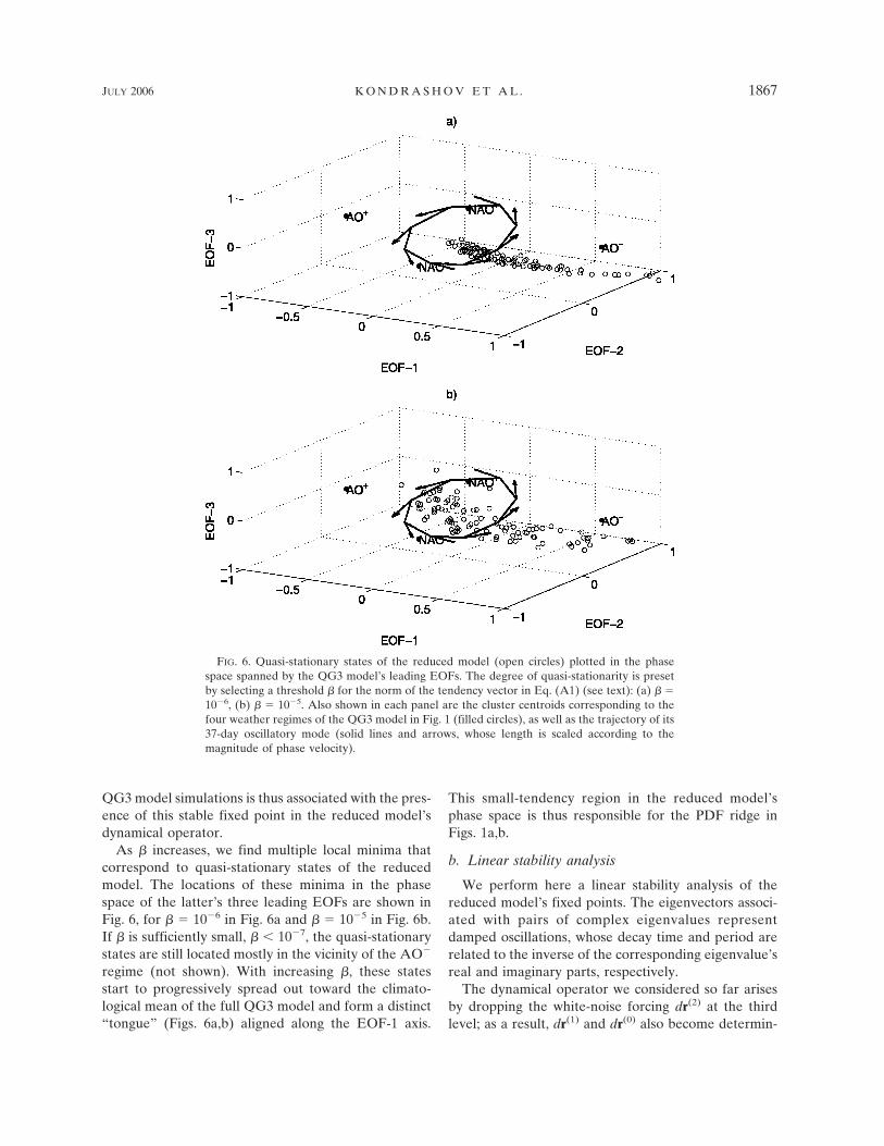
We visualize in Figs. 9a–d the linear mode’s evolu-tion during one-half of its 37-day oscillation cycle. Thisfigure shows one-to-one correspondence between thelinear eigenmode of the reduced model and the simu-

FIG. 8. Real and imaginary parts of a least-damped eigenmode of the reduced model linearized about (a), (b)climatology (i.e., the origin of the model anomalies’ phase space), and (c), (d) its single stable steady state (see alsoFig. 7). Positive contours are thick. The period of the eigenmodes is 37 days in (a), (b) and 35 days in (c), (d).


lated intraseasonal pattern of the full QG3 model inFig. 4. We conclude, therefore, that the QG3 model’s37-day intraseasonal oscillation is associated with thedamped linear eigenmode of the reduced model, ex-cited by the modes of the full model that are capturedby the stochastic forcing in the reduced one.

The power spectrum of the PCs is getting progres-sively whiter as the rank increases, while the spatialscale of the EOFs is getting smaller. In both the re-duced and QG3 model simulations, the intraseasonaloscillation has a large amplitude in the four leadingPCs, as indicated by the size of the streamfunctionanomalies in Fig. 4; the variance associated with thisoscillation is very small, though, for the higher-rankedEOFs 5–15 (not shown). The cluster-centroid patterns

in both the QG3 model and the reduced model (section3) also have essentially null projections onto EOFs 5–15(not shown here, but see Kondrashov et al. 2004). Thereduced model with only a few state vector variables atthe first level, though—say I � 4 variables instead ofthe 15 used in the reduced model of sections 3 and4—reproduces neither the period and spatial pattern ofthe QG3 model’s intraseasonal signal nor its PDF struc-ture (not shown).

Based on this evidence, we conclude that interactionsbetween the leading modes 1–4 of the system’s LFV, onthe one hand, and the intermediate modes representedby EOFs 5–15, on the other, are an essential contribu-tor to the system’s low-dimensional, leading-order dy-namics. Such interactions between low-frequency flow

FIG. 9. Evolution of the oscillatory eigenmode of Figs. 8a,b. (a)–(d) Patterns that are equidistant in time, duringone-half of the oscillation cycle. Positive contours are thick.


and intermediate modes may also be instrumental indetermining the region of phase space in which thedominant intraseasonal oscillation actually takes place(see Fig. 6), thus removing the degeneracy of the lead-ing eigenmodes of the reduced model’s linearizationwith respect to the shifts of the basic state along theEOF-1 axis (see Fig. 8 and its discussion above). Theseinteractions could also play a role in slowing down theintraseasonal oscillation’s trajectory in the vicinity ofthe anomalously persistent flow regimes detected insection 3c. Besides the intermediate modes 5–15, the“noise” associated with EOFs 16 and higher in the QG3model can also play a role in the system’s leading-orderdynamics, as we shall see forthwith.

c. Emergence of weather regimes

In this section, we track the emergence of the QG3model’s weather regimes. To do so, we introduce a fac-tor � (0 � � � 1) that multiplies the stochastic forcingterm dr(2) at the third level of the reduced model (see

the appendix), and perform simulations of the reducedmodel so modified using different values of �. For � �0, the solution converges to the steady state locatedwithin the AO� regime (see diamond in Fig. 7a andsection 4a). For small values of �, the stochastic forcingmerely causes the model trajectories to wander in thevicinity of this steady state. As the stochastic forcingamplitude � increases, the region occupied by the mod-el’s trajectory grows in size. As progressively largerportions of the phase space are filled up, the associatedPDF becomes more inhomogeneous.

In Figs. 10a–d, we show a mixture-model approxima-tion of this PDF, along with the clusters supported bythe simulated data for � � 0.2, 0.4, 0.6, and 1, respec-tively. The optimum number of clusters k* for eachvalue of � is obtained using the cross-validated log-likelihood criterion (Smyth et al. 1999; see also section2). For � � 0.15, k* � 1 (not shown), while k* increaseswith �: k* � 2 for � � 0.2 (Fig. 10a), k* � 3 for � � 0.4(Fig. 10b), and k* � 4 for � � 0.6 (Figs. 10c,d). This

FIG. 10. Mixture-model clusters for the reduced model simulations, in which the stochastic forcing is multipliedby a factor �: (a) � � 0.2, (b) � � 0.4, (c) � � 0.6, and (d) � � 1 (control case). Note that the number of clustersincreases with �.


increased non-Gaussianity of the model’s PDF is in-dicative of the weather regimes’ nonlinear origin, sincea linear system forced by Gaussian stochastic forcingwill always support only one mixture-model cluster,centered around the mean.

The AO� regime, characterized by a large positiveprojection onto EOF-1, is present in all of the reduced-model PDFs of Fig. 10 and is clearly related to thedeterministic model version’s steady state (see section4a). As � increases, the model PDF becomes elongatedin the negative EOF-1 direction (Figs. 10a,b), therebyspending most of the time in the vicinity of the quasi-stationary tongue of Fig. 6. As � increases even further(Figs. 10c,d), additional spreading of the PDF along theEOF-1 axis is accompanied by the PDF’s increased pro-jection onto the (EOF-2–EOF-3) plane (see Fig. 1c for� � 1; not shown for smaller �).

This increased three-dimensionality of the PDF is as-sociated with the excitation of the oscillatory modes ofsections 3b and 4b. The slow phases of the 37-day os-cillation, due to interactions between the model’s low-est-frequency EOFs (1–4) and faster (EOFs 5–15)modes (see sections 3c and 4b) become associated withthe emergence of additional anomalously persistent re-gimes. The latter occupy the vicinity of the model’sclimatological state, farther away from the three-levelreduced model’s unique steady state and AO� regime.

It is clear, therewith, that our reduced model doesnot support the oscillatory topographic instability ofGhil and associates (Legras and Ghil 1985; Jin and Ghil1990; Strong et al. 1993, 1995; Marcus et al. 1994, 1996)as a limit cycle (i.e., as a self-sustained, stable periodicsolution) of its empirically inferred, deterministic dy-namics. Instead, the 37-day oscillation arises here bythe reduced model’s stochastic forcing, which repre-sents the QG3 model’s eddy variability, pumping of aleast-damped eigenmode with the appropriate period-icity. This type of relation between episodic and oscil-latory variability in NH LFV, where synoptic variabilityplays a significant role, has to be added, therefore, tothe catalog of such relations already established by Ghilet al. (1991) and by Ghil and Robertson (2002).

5. Concluding remarks

a. Summary

We have constructed a reduced, nonlinear, stochas-tically forced model for the behavior of the three-level,quasigeostrophic (QG3) model with topography ofMarshall and Molteni (1993), using the empirical meth-odology of Kravtsov et al. (2005b). The QG3 model hasO(104) degrees of freedom. The reduced model, de-scribed in the appendix, operates in the phase space of

the QG3 model’s leading 15 empirical orthogonal func-tions (EOFs); it involves quadratic nonlinearity at thefirst model level, while the two additional levels, whichdescribe the effect of unresolved variables on the re-duced model’s evolution, are both linear (see section 2).

Our reduced model thus has 45 variables and isdriven at the third level by a spatially coherent noisethat is white in time. Once the size of the state vector(number of EOFs) is chosen, the number of levels inthe reduced model is determined automatically by en-suring that the last-level residual forcing’s lag-1 covari-ance matrix vanishes, while its lag-0 covariance matrixconverges to a constant matrix. The covariance matri-ces of the noise, as well as the model’s dynamical op-erator were determined from a very long simulation ofthe QG3 model, by least squares regression (Wetherill1986; Press et al. 1994; Kravtsov et al. 2005b). Ourmodel generalizes linear inverse models (LIMs), whichhave only one level and have been extensively appliedto study climate variability (Penland 1989, 1996; Pen-land and Ghil 1993; Penland and Sardeshmukh 1995;Penland and Matrosova 1998; Winkler et al. 2001).

The dimension I � 15 of EOF subspace for construct-ing the reduced model was chosen to maximize corre-spondence between its behavior and that of the fullQG3 model. We documented remarkable similarity be-tween the full and reduced models, in terms of theiranomalously persistent flow regimes, as described bythe Gaussian-mixture PDF (section 3a), and in terms oftheir low-frequency oscillatory modes, as captured bymultichannel singular-spectrum analysis (M-SSA; seesection 3b). The QG3 model’s low-frequency variability(LFV) in turn, captures several key features of ob-served NH LFV.

In particular, both models are characterized by fouranomalously persistent flow regimes, NAO�, NAO�,AO�, and AO� (see Figs. 1, 2 and section 3a), and adominant oscillatory mode with a period of about 37days (see Figs. 3, 4 and section 3b). The AO� andNAO� regimes are related, in both models, to anoma-lous slow-down of the intraseasonal oscillation trajec-tory, while AO� is a stand-alone regime (see Fig. 5 andsection 3c), also associated with the presence of thePDF ridge in Figs. 1a,b.

These features of both models’ LFV were interpretedvia the analysis of the reduced-model dynamics in sec-tion 4: the AO� regime arises from the unique steadystate of the reduced model’s 3-level deterministic op-erator, while the PDF ridge of Figs. 1a,b coincides withthe location of a plateau of quasi-stationary states ofthe reduced model (see Fig. 6 and section 4a). Asshown in section 4b, the dominant intraseasonal oscil-lation in both the QG3 and reduced model has a period


of about 35–37 days and is associated with the least-damped eigenmode of the latter (Fig. 7), when linear-ized about its climatological state (cf. Figs. 9 and 4).

This eigenmode is also very similar to the least-damped eigenmode obtained when linearizing the re-duced model’s deterministic operator about the AO�

steady state (cf. Figs. 8a,b and Figs. 8c,d). The similaritybetween the two eigenmodes reflects their approximateinvariance with respect to shifts of the basic state alongthe EOF-1 axis; the large degree of zonal symmetry ofEOF-1 helps explain such an invariance, which is alsoconsistent with the presence of the quasi-stationarytongue along this axis (Fig. 6).

The degeneracy associated with these shifts is re-moved due to interactions between the largest-scalemodes of the system, whose variance is concentrated inthe subspace of the four leading EOFs, and the inter-mediate scales, captured by EOFs 5–15; the reducedmodel constructed in the phase subspace of the fourleading EOFs alone reproduces neither the non-Gaussian features of the QG3 model’s PDF, nor itslow-frequency oscillatory modes. We also suspect,therefore, that such interactions are responsible for theslow-down of the intraseasonal oscillation’s trajectoryin the full QG3 model, as well as in our optimal reducedmodel; this slow-down is associated with the emergenceof the AO� and NAO� regimes.

Finally, in section 4c, we studied the emergence ofmultiple flow regimes and intraseasonal oscillations asthe stochastic forcing associated with unresolved small-scale processes increases from zero to its observedvalue (Fig. 10): the model trajectory is initially confinedto a small region near the three-level reduced model’sunique steady state and gradually fills up the quasi-stationary ridge along the EOF-1 axis of the reducedmodel. When the amplitude of the stochastic forcingbecomes large enough, the intraseasonal oscillatorymode is excited, resulting in the model’s PDF expand-ing in the EOF-2 and EOF-3 directions, while addi-tional quasi-stationary clusters appear.

b. Discussion

The methodology of mode reduction used in this pa-per is based solely on the statistical information con-tained in the model-generated dataset. D’Andrea andVautard (2001) and D’Andrea (2002) took a differentapproach and constructed a low-order representationof the QG3 model by projecting its equations onto afew leading EOFs of the model, and introducing anempirical deterministic closure to account for the effectof unresolved small-scale processes on the reducedmodel’s low-frequency evolution. They compared theperformance of the resulting deterministic low-order

model with that of the full QG3 model, in terms ofapproximate correspondence between the full model’sweather regimes and the quasi-stationary states of thelow-order model. Their flow-dependent parameteriza-tion of the closure term turned out to be essential for agood performance of the reduced model. In particular,their Arctic High regime, analogous to our AO� re-gime, had a high spatial correlation with the corre-sponding unstable steady state of their deterministicreduced model.

Our model accounts for small-scale processes by us-ing additional model levels that describe their effect onthe large-scale variables; the energy for the system’svariability is supplied by the stochastic forcing, whichrepresents the joint effect of small-scale instabilitiesthat occur in the full model. The AO� regime of theQG3 and reduced models is associated, in our ap-proach, with the unique steady state of the reducedmodel’s three-level deterministic operator. One canthink of this zonally symmetric regime as the zonal flowof classical dynamic meteorology (Gill 1982; Holton2004).

The correlation between the multiple-flow regimes’anomaly patterns in our reduced model and those ofthe full QG3 model all exceed 0.9 and are thus higherthan the correlations obtained by D’Andrea and Vau-tard (2001) and D’Andrea (2002). It is interesting thatmost of the LFV in the QG3 model and in NH obser-vations, including the AO�, NAO� and NAO� re-gimes, as well as the intraseasonal oscillations, occurfairly far away in phase space from the classical zonalflow of the AO� regime.

Majda et al. (1999, 2001, 2002, 2003) have developeda strategy for systematic mode reduction in determin-istic models that govern geophysical flows. This strat-egy has been recently applied to the analysis of a baro-tropic atmospheric model (Franzke et al. 2005) and tothe QG3 model (C. Franzke and A. Majda 2005, per-sonal communication). Our method, like that of Majdaand colleagues, results in a nonlinear deterministicmodel, driven by stochastic forcing. Unlike theirmethod, ours is completely empirical and has also beenapplied directly to NH geopotential height anomalies(Kravtsov et al. 2005b), as well as to sea surface tem-perature anomalies (Kondrashov et al. 2005). The simi-larities and differences between these two methods,when applying both to a fairly realistic atmosphericmodel, like QG3, are a matter of considerable interestand further investigation.

The number of variables in our reduced model ismuch less than the number of degrees of freedom in thefull QG3 model, but it is still larger than the number ofmodes that contain most of the latter models low-


frequency variance (EOFs 1–4). The higher-rankedEOFs 5–15 can thus be associated with intermediate-scale modes, while the additive noise in our reducedmodel’s highest level represents the smallest scales,captured by EOFs 16 and higher in the full QG3 model.Note that our higher-order PCs have spectra that be-come increasingly whiter, rather than being increas-ingly shifted to higher frequencies or faster decay times.

Direct comparison with the mode-reduction strategyof Majda and coauthors is thus difficult at the presentstage: our strategy emphasizes separation in spatialscales—large, intermediate, and small—while theirsemphasizes separation in temporal scales (somewhatlike in F. D’Andrea and R. Vautard’s work), with slowand fast scales only. This being said, there might besome analogy between the effects on the large-scaleLFV of the quadratic terms that describe the interac-tions between EOFs 1–4 and EOFs 5–15 in our reducedmodel, on the one hand, and the effects of multiplica-tive noise in the Franzke et al. (2005) model, on theother.

Empirically based reduced models, like the one con-structed in this paper, provide a useful statistical toolfor interpretation of complex behavior detected inhighly resolved climate models, as well as in observa-tions. Such models not only help compact the dataset’sinformation content but can also provide insights intothe dynamics of large-scale, low-frequency climate vari-ability, via the analysis of the reduced model’s math-ematical structure.

In this way, we have identified the leading modes ofthe QG3 model’s LFV as the least-damped eigenmodesof this system linearized about its climatological state(see also Branstator 1992, 1995; Farrell and Ioannou1993, 1995; Metz 1994; Da Costa and Vautard 1997;Itoh and Kimoto 1999; Kravtsov et al. 2003, 2005a). Wehave also pointed out the possible effect of the inter-mediate and smallest scales of motion on the QG3model’s LFV and on connecting the oscillatory descrip-tion of LFV with its “episodic” description via multipleflow regimes (Ghil et al. 1991; Ghil and Robertson2002). The effect of the smaller scales on the largestones may be related to a more or less active synopticeddy feedback (Robinson 1996, 2000; Lorenz and Hart-mann 2001, 2003; Koo et al. 2002; Kravtsov et al.2005a), although a detailed look at how the additionallevels of the reduced model affect the deterministic dy-namics indicates a damping role of the red-noise-likesmall scales in the QG3 model.

We have provided additional evidence for the AO�

regime, detected in the QG3-model simulation and as-sociated with the steady state of our reduced model,representing a dynamical entity that is distinct from the

regional NAO phenomenon (see also Deser 2000;Kravtsov et al. 2006). Our reduced-model analysis alsosuggests that extended-range predictability of the NAOmay be possible, due to its connection with intrasea-sonal oscillations (Lott et al. 2001, 2004a,b) and mul-tiple flow regimes (Ghil and Robertson 2002).

Finally, an important difference between linear andnonlinear reduced models concerns their ability tosimulate non-Gaussian PDFs and help predict transi-tions between different weather regimes. Yang andReinhold (1991) have reviewed earlier studies of ob-served NH LFV and shown that large-amplitude tran-sitions between quasi-stationary, persistent states play akey role in it. On the other hand, D’Andrea et al. (1998)have reviewed the performance of 15 general circula-tion models and found them to generally underestimatethe number and duration of blocking events, whilePelly and Hoskins (2003) found that forecasts of block-ing inception in advanced numerical weather predictionsystems still have no skill starting from a lead time of sixdays. Thus, if a reduced model can simulate a non-Gaussian PDF whose distinct Gaussians capture mul-tiple weather regimes present in NH LFV, then it mightalso have some helpful skill at predicting the breaks andonsets of these regimes.

Acknowledgments. We are grateful to F. D’Andreafor providing a numerical code for the QG3 model andinformation on its performance. A. W. Robertson andP. J. Smyth kindly provided the codes for the k-meansmethod and the Gaussian mixture model and advice ontheir implementation. C. Franzke and A. J. Majda gen-erously shared with us their preprint “Low-order sto-chastic mode reduction for a prototype atmosphericGCM” and related correspondence. Three refereesprovided interesting and constructive comments. Thisstudy was supported by NSF Grant ATM00-82131 (DKand MG), as well as by DOE Grant DE-FG02-04ER63881 (SK). Preliminary results of this investiga-tion were presented at the First Annual Assembly ofthe European Geosciences Union held in Nice, France,in April 2004, and at the Fifth AIMS Dynamical Sys-tems Conference in Pomona, California, in June 2004.

APPENDIX

Constructing the Reduced Model

The inverse stochastic counterpart of the QG3 modelis constructed in the phase space of I leading EOFs ofthe 500-hPa streamfunction anomaly field. If x � {xi} issuch a state vector of dimension I, then the multilevelquadratic inverse stochastic model has the general form(Kravtsov et al. 2005b)


dxi � �xTAix � bi�0 x � ci

�0 � r i�0 dt,

dr i�0 � bi

�1 �x, r�0 � dt � r i�1 dt,

dr i�1 � bi

�2 �x, r�0 , r�1 � dt � r i�2 dt,

· · ·dr i

�N � bi�N �x, r�0 , r �1 , . . . , r �N � dt � dr i

�N�1 , i � 1, I;

�A1

the matrices Ai, the rows b(n)i of the matrices B(n), n �

0, N and the components c(0)i of the vector c(0), as well

as the components r(n)i of each level’s residual forcing

r(n), n � 0, N � 1, are determined by general leastsquares (Wetherill 1986; Press et al. 1994).

Linear inverse models (LIMs; see section 2) are aparticular case of Eq. (A1) with only one level, N � 1,and with zero Ai and c(0). Including quadratic nonlin-earity at the first level of the multilevel model allowsone to account for processes characterized by non-Gaussian statistics. The stochastic forcing r(0) at thislevel, however, typically involves serial correlations andmight also depend on the modeled process x. We in-clude, therefore, an additional model level to expressthe time increments dr(0) as a linear function of an ex-tended state vector (x, r(0))T; in numerical practice,these increments are equivalent to the divided differ-ences of the residual forcing r(0).

Linear dependence is used at the second and higherlevels ones since the non-Gaussian statistics of the datahas already been captured by the first, nonlinear level.More levels are added, until the estimate of the Nthlevel’s residual r(N�1) becomes white in time, and itslag-0 correlation matrix converges to a constant matrix.With the addition of each level, we are accounting foradditional time-lag information, thereby squeezing outany time correlations from the residual forcing. Equa-tion (A1) thus describes a wide class of processes in afashion that explicitly accounts for the modeled processx feeding back on the noise statistics (see Kravtsov et al.2005b).

REFERENCES

Branstator, G. W., 1987: A striking example of the atmosphere’sleading traveling pattern. J. Atmos. Sci., 44, 2310–2323.

——, 1992: The maintenance of low-frequency atmosphericanomalies. J. Atmos. Sci., 49, 1924–1945.

——, 1995: Organization of storm track anomalies by recurringlow-frequency circulation anomalies. J. Atmos. Sci., 52, 207–226.

Cheng, X. H., and J. M. Wallace, 1993: Analysis of the northern-hemisphere wintertime 500-hPa height field spatial patterns.J. Atmos. Sci., 50, 2674–2696.

Coleman, T. F., and Y. Li, 1994: On the convergence of reflective

Newton methods for large-scale nonlinear minimization sub-ject to bounds. Math. Program., 67, 189–224.

——, and ——, 1996: An interior, trust region approach for non-linear minimization subject to bounds. SIAM J. Optim., 6,418–445.

Da Costa, E., and R. Vautard, 1997: A qualitative realistic low-order model of the extratropical low-frequency variabilitybuilt from long records of potential vorticity. J. Atmos. Sci.,54, 1064–1084.

D’Andrea, F., 2002: Extratropical low-frequency variability as alow-dimensional problem. Part II: Stationarity and stabilityof large-scale equilibria. Quart. J. Roy. Meteor. Soc., 128,1059–1073.

——, and R. Vautard, 2001: Extratropical low-frequency variabil-ity as a low-dimensional problem. Part I: A simplified model.Quart. J. Roy. Meteor. Soc., 127, 1357–1374.

——, and Coauthors, 1998: Northern Hemisphere atmosphericblocking as simulated by 15 general circulation models in theperiod 1979–1988. Climate Dyn., 14, 285–325.

Deser, C., 2000: On the teleconnectivity of the “Arctic Oscilla-tion.” Geophys. Res. Lett., 27, 779–782.

Dole, R. M., and N. D. Gordon, 1983: Persistent anomalies of theextratropical Northern Hemisphere wintertime circulation —Geographical distribution and regional persistence character-istics. Mon. Wea. Rev., 111, 1567–1586.

Farrell, B. F., and P. J. Ioannou, 1993: Stochastic forcing of thelinearized Navier–Stokes equations. Phys. Fluids, 5A, 2600–2609.

——, and ——, 1995: Stochastic dynamics of the midlatitude at-mospheric jet. J. Atmos. Sci., 52, 1642–1656.

Franzke, C., A. J. Majda, and E. Vanden-Eijnden, 2005: Low-order stochastic mode reduction for a realistic barotropicmodel climate. J. Atmos. Sci., 62, 1722–1745.

Ghil, M., and S. Childress, 1987: Topics in Geophysical Fluid Dy-namics: Atmospheric Dynamics, Dynamo Theory and ClimateDynamics. Springer-Verlag, 485 pp.

——, and K. C. Mo, 1991: Intraseasonal oscillations in the globalatmosphere. Part I: Northern Hemisphere and Tropics. J.Atmos. Sci., 48, 752–779.

——, and A. W. Robertson, 2000: Solving problems with GCMs:General circulation models and their role in the climate mod-eling hierarchy. General Circulation Model Development:Past, Present and Future, D. Randall, Ed., Academic Press,285–325.

——, and ——, 2002: “Waves” vs. “particles” in the atmosphere’sphase space: A pathway to long-range forecasting? Proc.Natl. Acad. Sci. USA, 99 (Suppl. 1), 2493–2500.

——, M. Kimoto, and J. D. Neelin, 1991: Nonlinear dynamics andpredictability in the atmospheric sciences. Rev. Geophys., 29,(Suppl.: U.S. National Rep. to Int. Union of Geodesy andGeophysics, 1987–1990), 46–55.

——, and Coauthors, 2002: Advanced spectral methods for cli-matic time series. Rev. Geophys., 40, 1003, doi:10.1029/2000GR000092.

Gill, A. E., 1982: Atmosphere–Ocean Dynamics. Academic Press,662 pp.

Hannachi, A., 1997: Low-frequency variability in a GCM: Three-dimensional flow regimes and their dynamics. J. Climate, 10,1357–1379.

——, and A. O’Neil, 2001: Atmospheric multiple equilibria andnon-Gaussian behavior in model simulations. Quart. J. Roy.Meteor. Soc., 127, 939–958.


Holton, J. R., 2004: An Introduction to Dynamic Meteorology. 4thed. Elsevier/Academic Press, 529 pp.

Hurrel, J. E., 1995: Decadal trends in the North Atlantic Oscilla-tion: Regional temperatures and precipitation. Science, 269,676–679.

Itoh, H., and M. Kimoto, 1999: Weather regimes, low-frequencyoscillations, and principal patterns of variability: A perspec-tive of extratropical low-frequency variability. J. Atmos. Sci.,56, 2684–2705.

Jin, F. F., and M. Ghil, 1990: Intraseasonal oscillations in the ex-tratropics: Hopf bifurcation and topographic instabilities. J.Atmos. Sci., 47, 3007–3022.

Johnson, S. D., D. S. Battisti, and E. S. Sarachik, 2000: Empiri-cally derived Markov models and prediction of tropical Pa-cific sea surface temperature anomalies. J. Climate, 13, 3–17.

Keppenne, C. L., and M. Ghil, 1993: Adaptive filtering and pre-diction of noisy multivariate signals: An application to sub-annual variability in atmospheric angular momentum. Intl. J.Bifurcation Chaos, 3, 625–634.

Kimoto, M., and M. Ghil, 1993a: Multiple flow regimes in theNorthern Hemisphere winter. Part I: Methodology and hemi-spheric regimes. J. Atmos. Sci., 50, 2625–2643.

——, and ——, 1993b: Multiple flow regimes in the NorthernHemisphere winter. Part II: Sectorial regimes and preferredtransitions. J. Atmos. Sci., 50, 2645–2673.

Kondrashov, D., K. Ide, and M. Ghil, 2004: Weather regimes andpreferred transition paths in a three-level quasigeostrophicmodel. J. Atmos. Sci., 61, 568–587.

——, S. Kravtsov, and M. Ghil, 2005: A hierarchy of data-basedENSO models. J. Climate, 18, 4425–4444.

Koo, S., A. W. Robertson, and M. Ghil, 2002: Multiple regimesand low-frequency oscillations in the Southern Hemisphere’szonal-mean flow. J. Geophys. Res., 107, doi:10.1029/2001JD001353.

Kravtsov, S., A. W. Robertson, and M. Ghil, 2003: Low-frequencyvariability in a baroclinic �-channel with land–sea contrast. J.Atmos. Sci., 60, 2267–2293.

——, ——, and ——, 2005a: Bimodal behavior in the zonal meanflow of a baroclinic �-channel model. J. Atmos. Sci., 62, 1746–1769.

——, D. Kondrashov, and M. Ghil, 2005b: Multilevel regressionmodeling of nonlinear processes: Derivation and applicationsto climatic variability. J. Climate, 18, 4404–4424.

——, A. W. Robertson, and M. Ghil, 2006: Multiple regimes andlow-frequency oscillations in the Northern Hemisphere’szonal-mean flow. J. Atmos. Sci., 63, 840–860.

Legras, B., and M. Ghil, 1985: Persistent anomalies, blocking andvariations in atmospheric predictability. J. Atmos. Sci., 42,433–471.

Lorenz, D. J., and D. L. Hartmann, 2001: Eddy–zonal flow feed-back in the Southern Hemisphere. J. Atmos. Sci., 58, 3312–3327.

——, and ——, 2003: Eddy–zonal flow feedback in the NorthernHemisphere winter. J. Climate, 16, 1212–1227.

Lott, F., A. W. Robertson, and M. Ghil, 2001: Mountain torquesand atmospheric oscillations. Geophys. Res. Lett., 28, 1207–1210.

——, ——, and ——, 2004a: Mountain torques and NorthernHemisphere low-frequency variability. Part I: Hemisphericaspects. J. Atmos. Sci., 61, 1259–1271.

——, ——, and ——, 2004b: Mountain torques and NorthernHemisphere low-frequency variability. Part II: Regional as-pects. J. Atmos. Sci., 61, 1272–1283.

Majda, A. J., I. Timofeyev, and E. Vanden-Eijnden, 1999: Modelsfor stochastic climate prediction. Proc. Natl. Acad. Sci. USA,96, 14 687–14 691.

——, ——, and ——, 2001: A mathematical framework for sto-chastic climate models. Commun. Pure Appl. Math., 54, 891–974.

——, ——, and ——, 2002: A priori test of a stochastic modereduction strategy. Physica D, 170, 206–252.

——, ——, and ——, 2003: Systematic strategies for stochasticmode reduction in climate. J. Atmos. Sci., 60, 1705–1722.

Marcus, S. L., M. Ghil, and J. O. Dickey, 1994: The extratropical40-day oscillation in the UCLA general circulation model.Part I: Atmospheric angular momentum. J. Atmos. Sci., 51,1431–1446.

——, ——, and ——, 1996: The extratropical 40-day oscillation inthe UCLA general circulation model. Part II: Spatial struc-ture. J. Atmos. Sci., 53, 1993–2014.

Marshall, J., and F. Molteni, 1993: Toward a dynamical under-standing of atmospheric weather regimes. J. Atmos. Sci., 50,1792–1818.

Metz, W., 1994: Singular modes and low-frequency atmosphericvariability. J. Atmos. Sci., 51, 1740–1753.

Mo, K., and M. Ghil, 1988: Cluster analysis of multiple planetaryflow regimes. J. Geophys. Res., 93D, 10 927–10 952.

Molteni, F., 2002: Weather regimes and multiple equilibria. En-cyclopedia of Atmospheric Science, J. R. Holton, J. Curry,and J. Pyle, Eds., Academic Press, 2577–2585.

Mukougawa, H., 1988: A dynamical model of “quasi-stationary”states in large-scale atmospheric motions. J. Atmos. Sci., 45,2868–2888.

Mundt, M. D., and J. E. Hart, 1994: Secondary instability, EOFreduction, and the transition to baroclinic chaos. Physica D,78, 65–92.

Pelly, J., and B. Hoskins, 2003: How well does the ECMWF en-semble prediction system predict blocking? Quart. J. Roy.Meteor. Soc., 129, 1683–1703.

Penland, C., 1989: Random forcing and forecasting using principaloscillation pattern analysis. Mon. Wea. Rev., 117, 2165–2185.

——, 1996: A stochastic model of Indo-Pacific sea-surface tem-perature anomalies. Physica D, 98, 534–558.

——, and M. Ghil, 1993: Forecasting Northern Hemisphere 700-mb geopotential height anomalies using empirical normalmodes. Mon. Wea. Rev., 121, 2355–2372.

——, and P. D. Sardeshmukh, 1995: The optimal growth of tropi-cal sea surface temperature anomalies. J. Climate, 8, 1999–2024.

——, and L. Matrosova, 1998: Prediction of tropical Atlantic seasurface temperatures using linear inverse modeling. J. Cli-mate, 11, 483–496.

Plaut, G., and R. Vautard, 1994: Spells of low-frequency variabil-ity and weather regimes in the Northern Hemisphere. J. At-mos. Sci., 51, 210–236.

Preisendorfer, R. W., 1988: Principal Component Analysis in Me-teorology and Oceanography. Elsevier, 425 pp.

Press, W. H., S. A. Teukolsky, W. T. Vetterling, and B. P. Flan-nery, 1994: Numerical Recipes. 2d ed. Cambridge UniversityPress, 994 pp.

Reinhold, B. B., and R. T. Pierrehumbert, 1982: Dynamics ofweather regimes: Quasi-stationary waves and blocking. Mon.Wea. Rev., 110, 1105–1145; Corrigendum, 113, 2055–2056

Rinne, J., and V. Karhila, 1975: A spectral barotropic model inhorizontal empirical orthogonal functions. Quart. J. Roy. Me-teor. Soc., 101, 365–382.


Robinson, W., 1996: Does eddy feedback sustain variability in thezonal index? J. Atmos. Sci., 53, 3556–3569.

——, 2000: A baroclinic mechanism for the eddy feedback on thezonal index. J. Atmos. Sci., 57, 415–422.

Schubert, S. D., 1985: A statistical–dynamical study of empiricallydetermined modes of atmospheric variability. J. Atmos. Sci.,42, 3–17.

Selten, F. M., 1995: An efficient description of the dynamics of thebarotropic flow. J. Atmos. Sci., 52, 915–936.

——, 1997: Baroclinic empirical orthogonal functions as basisfunctions in an atmospheric model. J. Atmos. Sci., 54, 2100–2114.

Sirovich, L., and J. D. Rodriguez, 1987: Coherent structures andchaos—A model problem. Phys. Lett., 120, 211–214.

Smyth, P., K. Ide, and M. Ghil, 1999: Multiple regimes in North-ern Hemisphere height fields via mixture model clustering. J.Atmos. Sci., 56, 3704–3723.

Strong, C. M., F.-F. Jin, and M. Ghil, 1993: Intraseasonal variabil-ity in a barotropic model with seasonal forcing. J. Atmos. Sci.,50, 2965–2986.

——, ——, and ——, 1995: Intraseasonal oscillations in a baro-tropic model with annual cycle, and their predictability. J.Atmos. Sci., 52, 2627–2642.

Thompson, D. W. J., and J. M. Wallace, 2000: Annular modes inthe extratropical circulation. Part I: Month-to-month vari-ability. J. Climate, 13, 1000–1016.

——, ——, and G. C. Hegerl, 2000: Annular modes in the extra-tropical circulation. Part II: Trends. J. Climate, 13, 1018–1036.

Vautard, R., and B. Legras, 1988: On the source of low frequencyvariability. Part II: Nonlinear equilibration of weather re-gimes. J. Atmos. Sci., 45, 2845–2867.

——, K.-C. Mo, and M. Ghil, 1990: Statistical significance test fortransition matrices of atmospheric Markov chains. J. Atmos.Sci., 47, 1926–1931.

Wallace, J. M., 2000: North Atlantic Oscillation/Annular Mode:Two paradigms–one phenomenon. Quart. J. Roy. Meteor.Soc., 126, 791–805.

——, and D. S. Gutzler, 1981: Teleconnections in the geopotentialheight field during the Northern Hemisphere winter. Mon.Wea. Rev., 109, 784–812.

Watanabe, M., 2004: Asian jet waveguide and a downstream ex-tension of the North Atlantic Oscillation. J. Climate, 17,4674–4691.

Wetherill, G. B., 1986: Regression Analysis with Applications.Chapman and Hall, 311 pp.

Winkler, C. R., M. Newman, and P. D. Sardeshmukh, 2001: Alinear model of wintertime low-frequency variability. Part I:Formulation and forecast skill. J. Climate, 14, 4474–4494.

Yang, S., and B. Reinhold, 1991: How does the low-frequencyvariance vary? Mon. Wea. Rev., 119, 119–127.


Empirical Mode Reduction in a Model of Extratropical … · Empirical Mode Reduction in a Model of...

Documents

Transcript of Empirical Mode Reduction in a Model of Extratropical … · Empirical Mode Reduction in a Model of...