Numerical solutions of 2-D steady incompressible flow

in a driven skewed cavity.

Ercan Erturk 1, Bahtiyar Dursun

Gebze Institute of Technology, Energy Systems Engineering Department, Gebze, Kocaeli 41400, Turkey

Key words Driven skewed cavity flow, steady incompressible N-S equations, general curvilinear coordinates, finite

difference, non-orthogonal grid mesh

AbstractThe benchmark test case for non-orthogonal grid mesh, the “driven skewed cavity flow”, first introduced by Demirdžiü et

al. [5] for skew angles of 30D D and 45D D , is reintroduced with a more variety of skew angles. The benchmark

problem has non-orthogonal, skewed grid mesh with skew angle (D ). The governing 2-D steady incompressible Navier-

Stokes equations in general curvilinear coordinates are solved for the solution of driven skewed cavity flow with non-

orthogonal grid mesh using a numerical method which is efficient and stable even at extreme skew angles. Highly

accurate numerical solutions of the driven skewed cavity flow, solved using a fine grid (512¯512) mesh, are presented

for Reynolds number of 100 and 1000 for skew angles ranging between15 165Dd dD D .

1. Introduction

In the literature, it is possible to find many numerical methods proposed for the solution of the steady

incompressible N-S equations. These numerical methods are often tested on several benchmark test cases in

terms of their stability, accuracy as well as efficiency. Among several benchmark test cases for steady

incompressible flow solvers, the driven cavity flow is a very well known and commonly used benchmark

problem. The reason why the driven cavity flow is so popular may be the simplicity of the geometry. In this

flow problem, when the flow variables are nondimensionalized with the cavity length and the velocity of the

lid, Reynolds number appears in the equations as an important flow parameter. Even though the geometry is

simple and easy to apply in programming point of view, the cavity flow has all essential flow physics with

counter rotating recirculating regions at the corners of the cavity. Among numerous papers found in the

literature, Erturk et al. [6], Botella and Peyret [4], Schreiber and Keller [21], Li et al. [12], Wright and Gaskel

[30], Erturk and Gokcol [7], Benjamin and Denny [2] and Nishida and Satofuka [16] are examples of

numerical studies on the driven cavity flow.

Due to its simple geometry, the cavity flow is best solved in Cartesian coordinates with Cartesian grid

mesh. Most of the benchmark test cases found in the literature have orthogonal geometries therefore they are

best solved with orthogonal grid mesh. However often times the real life flow problems have much more

complex geometries than that of the driven cavity flow. In most cases, researchers have to deal with non-

orthogonal geometries with non-orthogonal grid mesh. In a non-orthogonal grid mesh, when the governing

equations are formulated in general curvilinear coordinates, cross derivative terms appear in the equations.

Depending on the skewness of the grid mesh, these cross derivative terms can be very significant and can

affect the numerical stability as well as the accuracy of the numerical method used for the solution. Even

though, the driven cavity flow benchmark problem serves for comparison between numerical methods, the

flow is far from simulating the real life fluid problems with complex geometries with non-orthogonal grid

mesh. The numerical performances of numerical methods on orthogonal grids may or may not be the same on

non-orthogonal grids.

Unfortunately, there are not much benchmark problems with non-orthogonal grids for numerical methods

to compare solutions with each other. Demirdžiü et al. [5] have introduced the driven skewed cavity flow as a

test case for non-orthogonal grids. The test case is similar to driven cavity flow but the geometry is a

parallelogram rather than a square. In this test case, the skewness of the geometry can be easily changed by

1Corresponding author, e-mail: ercanerturk@gyte.edu.tr, URL: http://www.cavityflow.com

Published in : ZAMM - Journal of Applied Mathematics and Mechanics (2007)

ZAMM - Z. Angew. Math. Mech. 2007; Vol 87: pp 377-392

changing the skew angle (D ). The skewed cavity problem is a perfect test case for body fitted non-orthogonal

grids and yet it is as simple as the cavity flow in terms of programming point of view. Later Oosterlee et al.

[17], Louaked et al. [13], Roychowdhury et al. [20], Xu and Zhang [31], Wang and Komori [28], Xu and

Zhang [32], Tucker and Pan [27], Brakkee et al. [3], Pacheco and Peck [18], Teigland and Eliassen [25], Lai

and Yan [11] and Shklyar and Arbel [22] have solved the same benchmark problem. In all these studies, the

solution of the driven skewed cavity flow is presented for Reynolds numbers of 100 and 1000 for only two

different skew angles which are 30D D and 45D D and also the maximum number of grids used in these

studies is 320¯320.

Periü [19] considered the 2-D flow in a skewed cavity and he stated that the governing equations fail to

converge for 30D � D . The main motivation of this study is then to reintroduce the skewed cavity flow problem

with a wide range of skew angle (15 165Dd dD D ) and present detailed tabulated results obtained using a fine

grid mesh with 512¯512 points for future references.

Erturk et al. [6] have introduced an efficient, fast and stable numerical formulation for the steady

incompressible Navier-Stokes equations. Their methods solve the streamfunction and vorticity equations

separately, and the numerical solution of each equation requires the solution of two tridiagonal systems.

Solving tridiagonal systems are computationally efficient and therefore they were able to use very fine grid

mesh in their solution. Using this numerical formulation, they have solved the very well known benchmark

problem, the steady flow in a square driven cavity, up to Reynolds number of 21000 using a 601¯601 fine

grid mesh. Their formulation proved to be stable and effective at very high Reynolds numbers ([6], [7], [8]).

In this study, the numerical formulation introduced by Erturk et al. [6] will be applied to Navier-Stokes

equations in general curvilinear coordinates and the numerical solutions of the driven skewed cavity flow

problem with body fitted non-orthogonal skewed grid mesh will be presented. By considering a wide range of

skew angles, the efficiency of the numerical method will be tested for grid skewness especially at extreme

skew angles. The numerical solutions of the flow in a skewed cavity will be presented for Reynolds number of

100 and 1000 for a wide variety of skew angles ranging between 15D D and 165D D with

15D' D increments.

2. Numerical Formulation

For two-dimensional and axi-symmetric flows it is convenient to use the streamfunction (\ ) and vorticity

(Z ) formulation of the Navier-Stokes equations. In non-dimensional form, they are given as

xx yy\ \ Z� � (1)

( )y x x y xx yyRe

\ Z \ Z Z Z� �1

(2)

where, Re is the Reynolds number, and x and y are the Cartesian coordinates. We consider the governing

Navier-Stokes equations in general curvilinear coordinates as the following

( ) ( ) ( ) ( ) ( )x y x y xx yy xx yy x x y y[[ KK [ K [K[ [ \ K K \ [ [ \ K K \ [ K [ K \ Z� � � � � � � � � �2 2 2 22 (3)

( ) ( ) (( ) ( )x y x y x y x yRe

K [ [ K [[ KK[ K \ Z [ K \ Z [ [ Z K K Z� � � �2 2 2 21

( ) ( ) ( ) )xx yy xx yy x x y y[ K [K[ [ Z K K Z [ K [ K Z� � � � � �2 (4)

Following Erturk et al. [6], first pseudo time derivatives are assigned to streamfunction and vorticity equations

and using an implicit Euler time step for these pseudo time derivatives, the finite difference formulations in

operator notation become the following

2 2 2 2 1(1 ( ) ( ) ( ) ( ) ) n

x y x y xx yy xx yyt t t t[[ KK [ K[ [ G K K G [ [ G K K G \ ��' � �' � �' � �' �

( )n n n

x x y yt t[K\ [ K [ K \ Z � ' � � '2 (5)

( ( ) ( ) ( ) ( )x y x y xx yy xx yy

t t t t

Re Re Re Re[[ KK [ K[ [ G K K G [ [ G K K G

' ' ' '� � � � � � � �2 2 2 2

1

( ) ( ) )n n n

x y x yt tK [ [ K[ K \ G [ K \ G Z ��' � ' 1

( )n n

x x y y

t

Re[KZ [ K [ K Z

' � �

2 (6)

Where [[G and KKG denote the second order finite difference operators, and similarly [G and KG denote the

first order finite difference operators in [ - and K -direction respectively. The equations above are in implicit

form and require the solution of a large matrix at every pseudo time iteration which is computationally

inefficient. Instead these equations are spatially factorized such that

2 2 2 2 1(1 ( ) ( ) )(1 ( ) ( ) ) n

x y xx yy x y xx yyt t t t[[ [ KK K[ [ G [ [ G K K G K K G \ ��' � �' � �' � �' �

( )n n n

x x y yt t[K\ [ K [ K \ Z � ' � � '2 (7)

( ( ) ( ) ( ) )n

x y xx yy x y

t tt

Re Re[[ [ K [[ [ G [ [ G [ K \ G

' '� � � � � '2 2

1

( ( ) ( ) ( ) )n n

x y xx yy x y

t tt

Re ReKK K [ KK K G K K G [ K \ G Z �' '

u � � � � �'2 2 11

( )n n

x x y y

t

Re[KZ [ K [ K Z

' � �

2 (8)

The advantage of these equations are that each equation require the solution of a tridiagonal systems that can

be solved very efficiently using the Thomas algorithm. It can be shown that approximate factorization

introduces additional second order terms (O( t' 2 ))in these equations. In order for the equations to have the

correct physical representation, to cancel out the second order terms due to factorization the same terms are

added to the right hand side of the equations. The reader is referred to Erturk et al. [6] for more details of the

numerical method. The final form of the equations take the following form

2 2 2 2 1(1 ( ) ( ) )(1 ( ) ( ) ) n

x y xx yy x y xx yyt t t t[[ [ KK K[ [ G [ [ G K K G K K G \ ��' � �' � �' � �' �

( )n n n

x x y yt t[K\ [ K [ K \ Z � ' � � '2

2 2 2 2( ( ) ( ) )( ( ) ( ) ) n

x y xx yy x y xx yyt t t t[[ [ KK K[ [ G [ [ G K K G K K G \' � � ' � ' � � ' � (9)

( ( ) ( ) ( ) )n

x y xx yy x y

t tt

Re Re[[ [ K [[ [ G [ [ G [ K \ G

' '� � � � � '2 2

1

( ( ) ( ) ( ) )n n

x y xx yy x y

t tt

Re ReKK K [ KK K G K K G [ K \ G Z �' '

u � � � � �'2 2 11

( )n n

x x y y

t

Re[KZ [ K [ K Z

' � �

2

( ( ) ( ) ( ) )n

x y xx yy x y

t tt

Re Re[[ [ K [[ [ G [ [ G [ K \ G

' '� � � � '2 2

( ( ) ( ) ( ) )n n

x y xx yy x y

t tt

Re ReKK K [ KK K G K K G [ K \ G Z

' 'u � � � � '2 2

(10)

3. Driven Skewed Cavity Flow

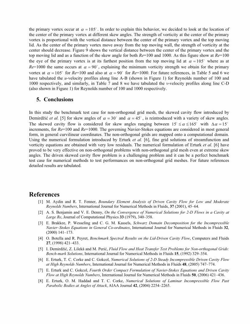
Fig. 1 illustrates the schematic view of the benchmark problem, the driven skewed cavity flow. We will

consider the most general case where the skew angle can be 90D ! D or 90D � D .

In order to calculate the metrics, the grids in the physical domain are mapped onto orthogonal grids in the

computational grids as shown in Fig. 2. The inverse transformation metrics are calculated using central

differences, as an example 1, 1,

12

1.

2 2

i j i jx x N

u N[� ��w :

w '

Similarly, inverse transformation metrics are

calculated as the following

, , ,cos sin

x x y yN N N

[ K [ KD D

1

0 (11)

where N is the number of grid points. We consider a (N¯N) grid mesh. The determinant of the Jacobian

matrix is found as

| |sin

J x y x yN

[ K K [D

� 2

(12)

The transformation metrics are defined as

, , ,| | | | | | | |

x y x yy x y xJ J J J

K K [ [[ [ K K� �

1 1 1 1

(13)

Substituting Equations (11) and (12) into (13), the transformation metrics are obtained as the following

, , ,x y x y

Ncos NN

sin sin

D[ [ K K

D D�

0 (14)

Note that since we use equal grid spacing, the second order transformation metrics will be all equal to zero

such that for example

( ) ( ) ( )x x xxx x x

x

[ [ [[ [ K

[ Kw w w

� w w w

0 (15)

Hence

xx yy xx yy[ [ K K 0 (16)

These calculated metrics are substituted into Equations (9) and (10) and the final form of the numerical

equations become as the following

( ( ) )( ( ) ) nN Nt t

sin sin[[ KKG G \

D D�� ' � '

2 21

2 21 1

cos( ) ( ( ) )( ( ) )n n n nN N N

t t t tsin sin sin

[K [[ KK

D\ \ Z G G \

D D D�

� ' � ' � ' '2 2 2

2 2 22 (17)

( ( ) ( ) )( ( ) ( ) )Re Re

n n nt N N t N Nt t

sin sin sin sin[[ K [ KK [ KG \ G G \ G Z

D D D D�' '

� � ' � �'2 2 2 2

1

2 2 2 21 1

( )n nt N cos

Re sin[K

DZ Z

D' �

�2

2

2

( ( ) ( ) )( ( ) ( ) )n n nt N N t N Nt t

Re sin sin Re sin sin[[ K [ KK [ KG \ G G \ G Z

D D D D' '

� �' � '2 2 2 2

2 2 (18)

The solution methodology of each of the above two equations, Equations (17) and (18), involves a two-stage

time-level updating. First the streamfunction equation (17) is solved, and for this, the variable f is introduced

such that

( ( ) ) nNt f

sinKKG \

D�� '

21

21 (19)

where

( ( ) ) ( )n n nN N cost f t t

sin sin[[ [K

DG \ \ Z

D D�

� ' � ' � '2 2

2 21 2

( ( ) )( ( ) ) nN Nt t

sin sin[[ KKG G \

D D� ' '

2 2

2 2 (20)

In Equation (20) f is the only unknown variable. First, this Equation (20) is solved for f at each grid point.

Following this, the streamfunction (\ ) variable is advanced into the new time level using Equation (19).

Then the vorticity equation (18) is solved, and in a similar fashion, the variable g is introduced such that

( ( ) ( ) )n nt N Nt g

Re sin sinKK [ KG \ G Z

D D�'

� � ' 2 2

1

21 (21)

where

( ( ) ( ) ) ( )n n nt N N t N cost g

Re sin sin Re sin[[ K [ [K

DG \ G Z Z

D D D' ' �

� � ' �2 2 2

2 2

21

( ( ) ( ) )( ( ) ( ) )n n nt N N t N Nt t

Re sin sin Re sin sin[[ K [ KK [ KG \ G G \ G Z

D D D D' '

� �' � '2 2 2 2

2 2 (22)

As with f , first the variable g is determined at every grid point using Equation (22), then vorticity (Z )

variable is advanced into the next time level using Equation (21).

3.1 Boundary Conditions

In the computational domain the velocity components are defined as the following

y y y

Ncos Nu

sin sin[ K [ K

D\ [ \ K \ \ \

D D�

� � (23)

x x xv N[ K [\ [ \ K \ \ � � � � (24)

On the left wall boundary we have

, , ,, | , |j j jK KK\ \ \ 0 0 0

0 0 0 (25)

where the subscripts 0 and j are the grid indexes. Also on the left wall, the velocity is zero (u 0 and v 0 ).

Using Equations (23) and (24) we obtain

,| j[\ 0

0 (26)

and also

,

( )| j

[[K

\\

K

w

w 0 0 (27)

Therefore, substituting these into the streamfunction Equation (3) and using Thom’s formula [26], on the left

wall boundary the vorticity is calculated as the following

,

,

j

j

N

sin

\Z

D �

2

1

0 2

2 (28)

Similarly the vorticity on the right wall (,N jZ ) and the vorticity on the bottom wall (

,0iZ ) are defined

as the following

, ,

, ,,N j i

N j i

N N

sin sin

\ \Z Z

D D� � �

2 2

1 1

02 2

2 2 (29)

On the top wall the u-velocity is equal to u 1 . Following the same procedure, the vorticity on the top wall is

found as

,

,

i N

i N

N N

sin sin

\Z

D D� � �

2

1

2

2 2 (30)

We note that, it is well understood ([10], [15], [23], [29]) that, even though Thom’s method is locally first

order accurate, the global solution obtained using Thom’s method preserves second order accuracy. Therefore

in this study, since three point second order central difference is used inside the skewed cavity and Thom’s

method is used at the wall boundary conditions, the presented solutions are second order accurate.

In the skewed driven cavity flow, the corner points are singular points for vorticity. We note that due to the

skew angle, the governing equations have cross derivative terms and because of these cross derivative terms

the computational stencil includes 3¯3 grid points. Therefore, the solution at the first diagonal grid points

near the corners of the cavity require the vorticity values at the corner points. For square driven cavity flow

Gupta et al. [9] have introduced an explicit asymptotic solution in the neighborhood of sharp corners.

Similarly, Störtkuhl et al. [24] have presented an analytical asymptotic solutions near the corners of cavity and

using finite element bilinear shape functions they also have presented a singularity removed boundary

condition for vorticity at the corner points as well as at the wall points. In this study we follow Störtkuhl et al.

[24] and use the following expression for calculating vorticity values at the corners of the skewed cavity

2

2

1 1 12 1

2 9 2 2sin3sin

1 1 11

2 2 4

N VN\ Z

DD

ª º ª º« » « »x x x x x x« » « »« » « »x � � x �« » « »« » « »« » « »x x¬ ¼ ¬ ¼

(31)

where V is the speed of the wall which is equal to 1 for the upper two corners and it is equal to 0 for the

bottom two corners. The reader is referred to Störtkuhl et al. [24] for details.

4. Results

The steady incompressible flow in a driven skewed cavity is numerically solved using the described numerical

formulation and boundary conditions. We have considered two Reynolds numbers, Re=100 and Re=1000. For

these two Reynolds numbers we have varied the skew-angle (D ) from 15D D 165D D with 15D' D

increments. We have solved the introduced problem with a 512¯512 grid mesh, for the two Reynolds number

and for all the skew angles considered.

During the iterations as a measure of the convergence to the steady state solution, we monitored three error

parameters. The first error parameter, ERR1 , is defined as the maximum absolute residual of the finite

difference equations of the steady streamfunction and vorticity equations in general curvilinear

coordinates, Equations (3) and (4). These are respectively given as

2 2 2

2 2 2

,

cos1 max abs 2

sin sin sin

n

i j

N N NERR

a a a\ [[ KK [K

D\ \ \ Z

§ ·§ ·¨ ¸¨ ¸ � � �

¨ ¸¨ ¸© ¹© ¹

2 2 2 2 2

2 2 2 2 2

,

1 1 2 cos1 max abs

sin sin sin sin sin

n

w

i j

N N N N NERR

Re a Re a a a Re a[[ KK K [ [ K [K

DZ Z \ Z \ Z Z

§ ·§ ·¨ ¸¨ ¸ � � � �

¨ ¸¨ ¸© ¹© ¹ (32)

The magnitude of ERR1 is an indication of the degree to which the solution has converged to steady state. In

the limit ERR1 would be zero.

The second error parameter, ERR2 , is defined as the maximum absolute difference between an iteration

time step in the streamfunction and vorticity variables. These are respectively given as

� �� �, ,max abs n n

i j i jERR \ \ \� �12

� �� �, ,max abs n n

i j i jERR Z Z Z� �12 (33)

ERR2 gives an indication of the significant digit of the streamfunction and vorticity variables are changing

between two time levels.

The third error parameter, ERR3 , is similar to ERR2 , except that it is normalized by the representative

value at the previous time step. This then provides an indication of the maximum percent change in \ and Zat each iteration step. ERR3 is defined as

, ,

,

max abs

n n

i j i j

n

i j

ERR \

\ \

\

�§ ·§ ·� ¨ ¸¨ ¸¨ ¸¨ ¸© ¹© ¹

1

3

, ,

,

max abs

n n

i j i j

n

i j

ERR Z

Z Z

Z

�§ ·§ ·� ¨ ¸¨ ¸¨ ¸¨ ¸© ¹© ¹

1

3 (34)

In our computations, for every Reynolds numbers and for every skew angles, we considered that convergence

was achieved when both ERR \1 and ERR Z1 were less than 1010� . Such a low value was chosen to ensure the

accuracy of the solution. At these residual levels, the maximum absolute difference in streamfunction value

between two time steps, ERR \2 , was in the order of 1710� and for vorticity, ERR Z2 , it was in the order of

1510� . And also at these convergence levels, between two time steps the maximum absolute normalized

difference in streamfunction, ERR \3 , and in vorticity, ERR Z3 , was in the order of 1410� , and 1310�

respectively.

We note that at extreme skew angles, convergence to such low residuals is necessary. For example, at skew

angle 15D D at the bottom left corner, and at skew angle 165D D at the bottom right corner, there appears

progressively smaller counter rotating recirculating regions in accordance with Moffatt [14]. In these

recirculating regions confined in the sharp corner, the value of streamfunction variable is getting extremely

smaller as the size of the recirculating region gets smaller towards the corner. Therefore, it is crucial to have

convergence to such low residuals especially at extreme skew angles.

Before solving the skewed driven cavity flow at different skew angles first we have solved the square

driven cavity flow to test the accuracy of the solution. The square cavity is actually a special case for skewed

cavity and obtained when the skew angle is chosen as 90D D . For the square driven cavity flow, the

streamfunction and the vorticity values at the center of the primary vortex and the location of this center are

tabulated in Table 1 for Reynolds numbers of Re=1000, together with results found in the literature. The

present results are almost exactly the same with that of Erturk et al. [6]. This was expected since in both

studies the same number of grid points were used and also the spatial accuracy of both the boundary condition

approximations and the solutions were the same. Furthermore the presented results are in very good agreement

with that of highly accurate spectral solutions of Botella and Peyret [4] and extrapolated solutions of Schreiber

and Keller [21] and also fourth order solutions of Erturk and Gokcol [7] with approximately less than 0.18%

and 0.14% difference in streamfunction and vorticity variables respectively. For all the skew angles considered

in this study (15 165Dd dD D )we expect to have the same level of accuracy we achieved forc. With Li et al.

[12], Wright and Gaskel [30], Benjamin and Denny [2] and Nishida and Satofuka [16] again our solutions

compare good.

After validating our solution for 90D D , we decided to validate our solutions at different skew angles. In

order to do this we compare our results with the results found in the literature. At this point, we would like to

note that in the literature among the studies that have solved the skewed cavity flow ([5], [17], [13], [20], [31],

[28], [32], [27], [3], [18], [25], [11] and [22]), only Demirdžiü et al. [5], Oosterlee et al. [17], Shklyar and

Arbel [22] and Louaked et al. [13] have presented tabulated results therefore we will mainly compare our

results with those studies.

As mentioned earlier, Demirdžiü et al. [5] have presented solutions for skewed cavity for Reynolds number

of 100 and 1000 for skewed angles of 45D D and 30D D . Figure 3 compares our results of u-velocity along

line A-B and v-velocity along line C-D with that of Demirdžiü et al. [5] for Re=100 and 1000 for 45D D , and

also Figure 4 compares the same for 30D D . Our results agree excellent with results of Demirdžiü et al. [5].

Table 2 compares our results of the minimum and also maximum streamfunction value and also their

location for Reynolds numbers of 100 and 1000 for skew angles of 30D D and 45D D with results of

Demirdžiü et al. [5], Oosterlee et al. [17], Louaked et al. [13] and Shklyar and Arbel [22]. The results of this

study and the results of Demirdžiü et al. [5] and also those of Oosterlee et al. [17], Shklyar and Arbel [22] and

Louaked et al. [13] agree well with each other, although we believe that our results are more accurate since in

this study a very fine grid mesh is used.

Figure 5 to Figure 8 show the streamline and also vorticity contours for Re=100 and Re=1000 for skew

angles from 15D D to 165D D with 15D' D increments. As it is seen from these contour figures of

streamfunction and vorticity, the solutions obtained are very smooth without any wiggles in the contours even

at extreme skew angles.

We have solved the incompressible flow in a skewed driven cavity numerically and compared our

numerical solution with the solutions found in the literature for 90D D , 30D and 45D , and good agreement is

found. We, then, have presented solutions for 15 165Dd dD D . Since we could not find solutions in the

literature to compare with our presented solutions other than 90D D , 30D and 45D , in order to demonstrate the

accuracy of the numerical solutions we presented, a good mathematical check would be to check the continuity

of the fluid, as suggested by Aydin and Fenner [1]. We have integrated the u-velocity and v-velocity profiles

along line A-B and line C-D, passing through the geometric center of the cavity shown by the red dotted line

in Figure 1, in order to obtain the net volumetric flow rate through these sections. Through section A-B, the

volumetric flow rate isABQ udy vdx �³ ³ and through section C-D it is

CDQ vdx ³ . Since the flow is

incompressible, the net volumetric flow rate passing through these sections should be equal to zero, 0Q .

Using Simpson’s rule for the integration, the volumetric flow ratesABQ and

CDQ are calculated for every skew

angle (D ) and every Reynolds number considered. In order to help quantify the errors, the obtained

volumetric flow rate values are normalized by the absolute total flow rate through the corresponding section at

the considered Re and D . Hence ABQ is normalized by u dy vdx�³ ³ and similarly

CDQ is normalized by

CDQ vdx ³ . Table 3 tabulates the normalized volumetric flow rates through the considered sections. We note

that in an integration process the numerical errors will add up, nevertheless, the normalized volumetric flow

rate values tabulated in Table 3 are close to zero, such that they can be considered as 0AB CDQ Q| | . This

mathematical check on the conservation of the continuity shows that our numerical solution is indeed very

accurate at the considered skew angles and Reynolds numbers.

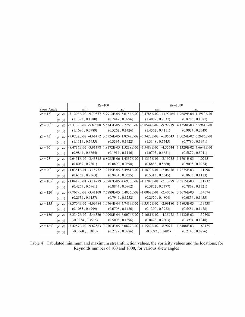
We note that, to the authors best knowledge, in the literature there is not a study that considered the skewed

cavity flow at the skew angles used in the present study other than 30D D and 45D D . The solutions

presented in this study are unique therefore, for future references, in Table 4 we have tabulated the minimum

and also maximum streamfunction values and their locations and also the vorticity value at these points for

Reynolds number of 100 and 1000 for all the skew angles considered, from 15D D to 165D D with

15D' D increments. In this table the interesting point is, at Reynolds number of 1000, the strength of

vorticity (absolute value of the vorticity) at the center of the primary vortex decrease as the skew angle

increase from 15D D to 90D D , having the minimum value at 90D D . As the skew angle increase further

from 90D D to 165D D , the strength of vorticity at the center of the primary vortex increase. At this

Reynolds number, Re=1000, the streamfunction value at the center of the primary vortex also show the same

type of behavior, where the value of the streamfunction start to increase as the skew angle increase until

90D D , then start to decrease as the skew angle increase further. However at Reynolds number of 100, the

minimum value of the strength of vorticity and also the maximum value of the streamfunction at the center of

the primary vortex occur at 105D D . In order to explain this behavior, we decided to look at the location of

the center of the primary vortex at different skew angles. The strength of vorticity at the center of the primary

vortex is proportional with the vertical distance between the center of the primary vortex and the top moving

lid. As the center of the primary vortex move away from the top moving wall, the strength of vorticity at the

center should decrease. Figure 9 shows the vertical distance between the center of the primary vortex and the

top moving lid and as a function of the skew angle for both Re=100 and 1000. As this figure show at Re=100

the eye of the primary vortex is at its farthest position from the top moving lid at 105D D where as at

Re=1000 the same occurs at 90D D , explaining the minimum vorticity strength we obtain for the primary

vortex at 105D D for Re=100 and also at 90D D for Re=1000. For future references, in Table 5 and 6 we

have tabulated the u-velocity profiles along line A-B (shown in Figure 1) for Reynolds number of 100 and

1000 respectively, and similarly, in Table 7 and 8 we have tabulated the v-velocity profiles along line C-D

(also shown in Figure 1) for Reynolds number of 100 and 1000 respectively.

5. Conclusions

In this study the benchmark test case for non-orthogonal grid mesh, the skewed cavity flow introduced by

Demirdžiü et al. [5] for skew angles of 30D D and 45D D , is reintroduced with a variety of skew angles.

The skewed cavity flow is considered for skew angles ranging between 15 165Dd dD D with 15D' D

increments, for Re=100 and Re=1000. The governing Navier-Stokes equations are considered in most general

form, in general curvilinear coordinates. The non-orthogonal grids are mapped onto a computational domain.

Using the numerical formulation introduced by Erturk et al. [6], fine grid solutions of streamfunction and

vorticity equations are obtained with very low residuals. The numerical formulation of Erturk et al. [6] have

proved to be very effective on non-orthogonal problems with non-orthogonal grid mesh even at extreme skew

angles. The driven skewed cavity flow problem is a challenging problem and it can be a perfect benchmark

test case for numerical methods to test performances on non-orthogonal grid meshes. For future references

detailed results are tabulated.

References[1] M. Aydin and R. T. Fenner, Boundary Element Analysis of Driven Cavity Flow for Low and Moderate

Reynolds Numbers, International Journal for Numerical Methods in Fluids, 37 (2001), 45–64.

[2] A. S. Benjamin and V. E. Denny, On the Convergence of Numerical Solutions for 2-D Flows in a Cavity at

Large Re, Journal of Computational Physics 33 (1979), 340–358.

[3] E. Brakkee, P. Wesseling and C. G. M. Kassels, Schwarz Domain Decomposition for the Incompressible Navier–Stokes Equations in General Co-ordinates, International Journal for Numerical Methods in Fluids 32,

(2000) 141–173.

[4] O. Botella and R. Peyret, Benchmark Spectral Results on the Lid-Driven Cavity Flow, Computers and Fluids

27, (1998) 421–433.

[5] I. Demirdžiü, Z. Lileký and M. Periü, Fluid Flow and Heat Transfer Test Problems for Non-orthogonal Grids:

Bench-mark Solutions, International Journal for Numerical Methods in Fluids 15, (1992) 329–354.

[6] E. Erturk, T. C. Corke and C. Gokcol, Numerical Solutions of 2-D Steady Incompressible Driven Cavity Flow

at High Reynolds Numbers, International Journal for Numerical Methods in Fluids 48, (2005) 747–774.

[7] E. Erturk and C. Gokcol, Fourth Order Compact Formulation of Navier-Stokes Equations and Driven Cavity Flow at High Reynolds Numbers, International Journal for Numerical Methods in Fluids 50, (2006) 421–436.

[8] E. Erturk, O. M. Haddad and T. C. Corke, Numerical Solutions of Laminar Incompressible Flow Past Parabolic Bodies at Angles of Attack, AIAA Journal 42, (2004) 2254–2265.

[9] M. M. Gupta, R. P. Manohar and B. Noble, Nature of Viscous Flows Near Sharp Corners, Computers and

Fluids 9, (1981) 379–388.

[10] H. Huang and B. R. Wetton, Discrete Compatibility in Finite Difference Methods for Viscous Incompressible Fluid Flow, Journal of Computational Physics 126, (1996) 468–478.

[11] H. Lai and Y. Y. Yan, The Effect of Choosing Dependent Variables and Cellface Velocities on Convergence of

the SIMPLE Algorithm Using Non-Orthogonal Grids, International Journal of Numerical Methods for Heat &

Fluid Flow 11, (2001) 524–546.

[12] M. Li, T. Tang and B. Fornberg, A Compact Forth-Order Finite Difference Scheme for the Steady

Incompressible Navier-Stokes Equations International Journal for Numerical Methods in Fluids 20, (1995)

1137–1151.

[13] M. Louaked, L. Hanich and K. D. Nguyen, An Efficient Finite Difference Technique For Computing Incompressible Viscous Flows, International Journal for Numerical Methods in Fluids 25, (1997) 1057–1082.

[14] H. K. Moffatt, Viscous and resistive eddies near a sharp corner, Journal of Fluid Mechanics 18, (1963) 1–18.

[15] M. Napolitano, G. Pascazio and L. Quartapelle, A Review of Vorticity Conditions in the Numerical Solution of

the ] -\ Equations, Computers and Fluids 28, (1999) 139–185.

[16] H. Nishida and N. Satofuka, Higher-Order Solutions of Square Driven Cavity Flow Using a Variable-Order

Multi-Grid Method, International Journal for Numerical Methods in Fluids 34, (1992) 637–653.

[17] C. W. Oosterlee, P. Wesseling, A. Segal and E. Brakkee, Benchmark Solutions for the Incompressible Navier-

Stokes Equations in General Co-ordinates on Staggered Grids, International Journal for Numerical Methods in

Fluids 17, (1993) 301–321.

[18] J. R. Pacheco and R. E. Peck, Nonstaggered Boundary-Fitted Coordinate Method For Free Surface Flows,

Numerical Heat Transfer Part B 37, (2000) 267–291.

[19] M. Periü, Analysis of Pressure-Velocity Coupling on Non-orthogonal Grids, Numerical Heat Transfer Part B

17, (1990) 63–82.

[20] D. G. Roychowdhury, S. K. Das and T. Sundararajan, An Efficient Solution Method for Incompressible N-S

Equations Using Non-Orthogonal Collocated Grid, International Journal for Numerical Methods in

Engineering 45, (1999) 741–763.

[21] R. Schreiber and H. B. Keller, Driven Cavity Flows by Efficient Numerical Techniques, Journal of

Computational Physics 49, (1983) 310–333.

[22] A. Shklyar and A. Arbel, Numerical Method for Calculation of the Incompressible Flow in General

Curvilinear Co-ordinates With Double Staggered Grid, International Journal for Numerical Methods in Fluids

41, (2003) 1273–1294.

[23] W. F. Spotz, Accuracy and Performance of Numerical Wall Boundary Conditions for Steady 2D

Incompressible Streamfunction Vorticity, International Journal for Numerical Methods in Fluids 28, (1998)

737–757.

[24] T. Stortkuhl, C. Zenger and S. Zimmer, An Asymptotic Solution for the Singularity at the Angular Point of the

Lid Driven Cavity, International Journal of Numerical Methods for Heat & Fluid Flow 4, (1994) 47–59.

[25] R. Teigland and I. K. Eliassen, A Multiblock/Multilevel Mesh Refinement Procedure for CFD Computations,

International Journal for Numerical Methods in Fluids 36, (2001) 519–538.

[26] A. Thom, The Flow Past Circular Cylinders at Low Speed, Proceedings of the Royal Society of London Series

A 141, (1933) 651–669.

[27] P. G. Tucker and Z. Pan, A Cartesian Cut Cell Method for Incompressible Viscous Flow, Applied

Mathematical Modelling 24, (2000) 591–606.

[28] Y. Wang and S. Komori, On the Improvement of the SIMPLE-Like method for Flows with Complex Geometry,

Heat and Mass Transfer 36, (2000) 71–78.

[29] E. Weinan and L. Jian-Guo, Vorticity Boundary Condition and Related Issues for Finite Difference Schemes,

Journal of Computational Physics 124, (1996) 368–382.

[30] N. G. Wright and P. H. Gaskell, An Efficient Multigrid Approach to Solving Highly Recirculating Flows,

Computers and Fluids 24, (1995) 63–79.

[31] H. Xu and C. Zhang, Study Of The Effect Of The Non-Orthogonality For Non-Staggered Grids—The Results,

International Journal for Numerical Methods in Fluids 29, (1999) 625–644.

[32] H. Xu and C. Zhang, Numerical Calculation of Laminar Flows Using Contravariant Velocity Fluxes,

Computers and Fluids 29, (2000) 149–177.

a) skewed cavity with D�!���R

D�����R�

U = 1

d = 1

D�!���R�

d = 1

A

B

DC

U = 1

d = 1

d = 1

C

B

A

D

b) skewed cavity with D�����R

Fig. 1. Schematic view of driven skewed cavity flow

Fig

. 2

. T

ran

sfo

rmat

ion

of

the

ph

ysi

cal

do

mai

n t

o c

om

pu

tati

on

al d

om

ain

-1

x

y

[�

K�

i+1,j

i,j

01

-11

°° ¿°° ¾½

°° ¯°° ®­ wwww

»»»» ¼º

«««« ¬ª

wwww

wwww

°° ¿°° ¾½

°° ¯°° ®­ wwww

K[K

[

K[

yy

xx

yx

°° ¿°° ¾½

°° ¯°° ®­ wwww

»»»» ¼º

«««« ¬ª

wwww

wwww

°° ¿°° ¾½

°° ¯°° ®­ wwww

yxy

x

yx

KK

[[

K[

Co

mp

uta

tio

nal

do

mai

n

Ph

ysi

cal

do

mai

n

Di-1

,j

i,j-

1

i,j+

1

x'

=

N1

N1

y'

=

N

)(

sinD

['

=1

K'

=1

Re=100 α=45ο Re=100 α=45

ο

Re=1000 α=45οRe=1000 α=45

ο

grid index along C-D

v-velocity

0 128 256 384 512-0.2

-0.15

-0.1

-0.05

0

0.05

0.1

0.15

ComputedDemirdzic et al. (1992)

^

′

grid index along C-D

v-velocity

0 128 256 384 512-0.06

-0.05

-0.04

-0.03

-0.02

-0.01

0

0.01

0.02

0.03

ComputedDemirdzic et al. (1992)

^

′

u-velocity

grid

index

along

A-B

-0.25 0 0.25 0.5 0.75 10

128

256

384

512

ComputedDemirdzic et al. (1992)

^

′

u-velocity

grid

index

along

A-B

-0.25 0 0.25 0.5 0.75 10

128

256

384

512

ComputedDemirdzic et al. (1992)

^

′

Fig. 3. Comparison of u-velocity along line A-B and v-velocity alongline C-D, for Re=100 and 1000, for skew angle α=45

ο

Re=100 α=30ο Re=100 α=30

ο

Re=1000 α=30ο Re=1000 α=30

ο

u-velocity

grid

index

along

A-B

-0.25 0 0.25 0.5 0.75 10

128

256

384

512

ComputedDemirdzic et al. (1992)

^

′

grid index along C-D

v-velocity

0 128 256 384 512-0.15

-0.1

-0.05

0

0.05

0.1

0.15

Computed

^

′Demirdzic et al. (1992)

u-velocity

grid

index

along

A-B

-0.25 0 0.25 0.5 0.75 10

128

256

384

512

ComputedDemirdzic et al. (1992)

^

′

grid index along C-D

v-velocity

0 128 256 384 512-0.03

-0.025

-0.02

-0.015

-0.01

-0.005

0

0.005

0.01

0.015

ComputedDemirdzic et al. (1992)

^

′

Fig. 4. Comparison of u-velocity along line A-B and v-velocity alongline C-D, for Re=100 and 1000, for skew angle α=30

ο

α

Verticaldistance

015

3045

6075

9010

512

013

515

016

518

00.

00

0.10

0.20

0.30

0.40

0.50

a)R

e=10

0b)

Re=

1000

α

Verticaldistance

015

3045

6075

9010

512

013

515

016

518

00.

05

0.10

0.15

0.20

0.25

0.30

Fig

.9.

The

vert

ical

dist

ance

betw

een

the

cent

erof

the

prim

ary

vort

exan

dth

eto

pm

ovin

glid

vers

usth

esk

ewan

gle

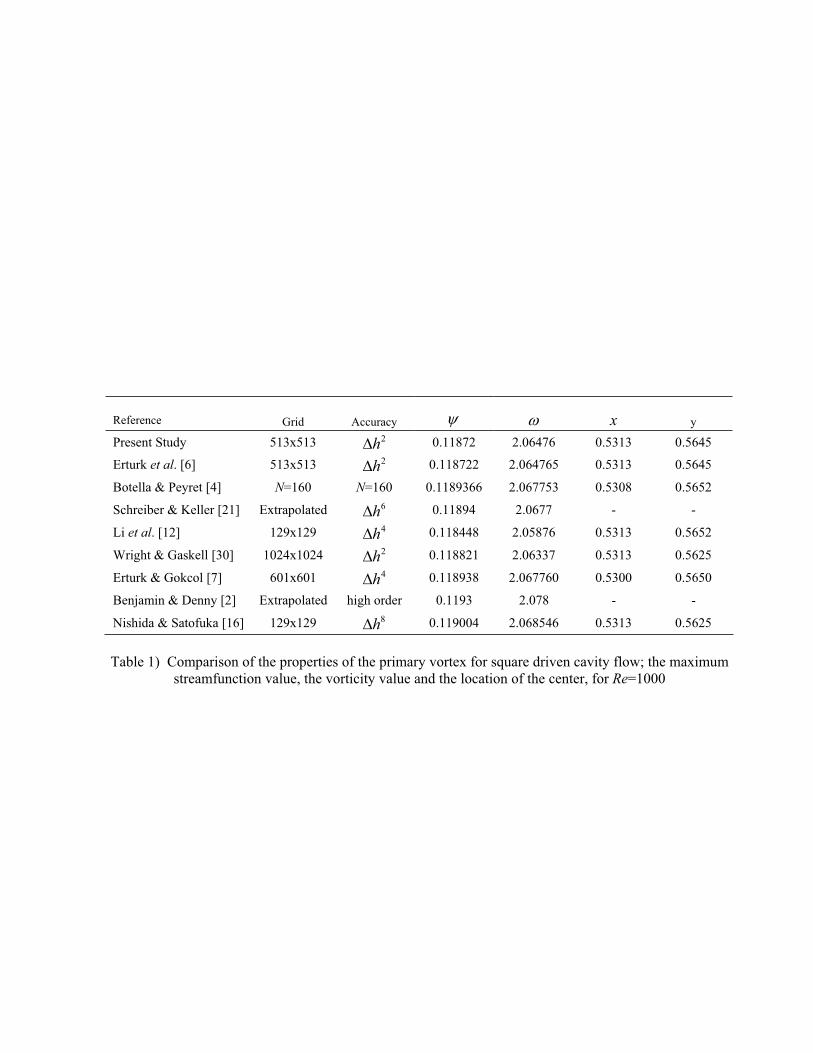
Reference Grid Accuracy \ Z x y

Present Study 513x513 2h' 0.11872 2.06476 0.5313 0.5645

Erturk et al. [6] 513x513 2h' 0.118722 2.064765 0.5313 0.5645

Botella & Peyret [4] N=160 N=160 0.1189366 2.067753 0.5308 0.5652

Schreiber & Keller [21] Extrapolated 6h' 0.11894 2.0677 - -

Li et al. [12] 129x129 4h' 0.118448 2.05876 0.5313 0.5652

Wright & Gaskell [30] 1024x1024 2h' 0.118821 2.06337 0.5313 0.5625

Erturk & Gokcol [7] 601x601 4h' 0.118938 2.067760 0.5300 0.5650

Benjamin & Denny [2] Extrapolated high order 0.1193 2.078 - -

Nishida & Satofuka [16] 129x129 8h' 0.119004 2.068546 0.5313 0.5625

Table 1) Comparison of the properties of the primary vortex for square driven cavity flow; the maximum

streamfunction value, the vorticity value and the location of the center, for Re=1000

Skew Re=100 Re=1000

Angle min max min max

Present study \ -5.3139E-02 5.5343E-05 -3.8544E-02 4.1358E-03

(513¯513) (x,y) (1.1680 , 0.3789) (0.5262 , 0.1426) (1.4562 , 0.4111) (0.9024 , 0.2549)

Demirdžiü et al. [5] \ -5.3135E-02 5.6058E-05 -3.8563E-02 4.1494E-03

(320¯320) (x,y) (1.1664 , 0.3790) (0.5269 , 0.1433) (1.4583 , 0.4109) (0.9039 , 0.2550)

30D D Oosterlee et al. [17] \ -5.3149E-02 5.6228E-05 -3.8600E-02 4.1657E-03

(256¯256) (x,y) (1.1680 , 0.3789) (0.5291 , 0.1426) (1.4565 , 0.4102) (0.9036 , 0.2559)

Shklyar and Arbel [22] \ -5.3004E-02 5.7000E-05 -3.8185E-02 3.8891E-03

(320¯320) (x,y) (1.1674 , 0.3781) (0.5211 , 0.1543) (1.4583 , 0.4109) (0.8901 , 0.2645)

Louaked et al. [13] \ - - -3.9000E-02 4.3120E-03

(120¯120) (x,y) - - (1.4540 , 0.4080) (0.8980 , 0.2560)

Present study \ -7.0232E-02 3.6724E-05 -5.3423E-02 1.0024E-02

(513¯513) (x,y) (1.1119 , 0.5455) (0.3395 , 0.1422) (1.3148 , 0.5745) (0.7780 , 0.3991)

Demirdžiü et al. [5] \ -7.0226E-02 3.6831E-05 -5.3507E-02 1.0039E-02

(320¯320) (x,y) (1.1100 , 0.5464) (0.3387 , 0.1431) (1.3130 , 0.5740) (0.7766 , 0.3985)

45D D Oosterlee et al. [17] \ -7.0238E-02 3.6932E-05 -5.3523E-02 1.0039E-02

(256¯256) (x,y) (1.1100 , 0.5469) (0.3390 , 0.1409) (1.3128 , 0.5745) (0.7775 , 0.4005)

Shklyar and Arbel [22] \ -7.0129E-02 3.9227E-05 -5.2553E-02 1.0039E-02

(320¯320) (x,y) (1.1146 , 0.5458) (0.3208 , 0.1989) (1.3120 , 0.5745) (0.7766 , 0.3985)

Louaked et al. [13] \ - - -5.4690E-02 1.0170E-02

(120¯120) (x,y) - - (1.3100 , 0.5700) (0.7760 , 0.3980)

Table 2) Comparison of the minimum and maximum streamfunction value and the location of these points,

for Reynolds number of 100 and 1000, for skew angles of 30D and 45D

AB

udy vdxQ

u dy v dx

�

�

³ ³³ ³

CD

vdxQ

v dx ³³

Skew

Angle Re=100 Re=1000 Re=100 Re=1000

D =15° 1.999E-05 2.275E-05 1.699E-05 7.794E-05

D =30° 2.089E-05 4.485E-05 2.692E-05 9.423E-06

D =45° 2.056E-05 5.841E-05 2.976E-05 1.552E-05

D =60° 2.054E-05 3.660E-05 2.225E-05 2.112E-06

D =75° 2.172E-05 3.849E-05 1.065E-05 1.371E-05

D =90° 2.420E-05 5.096E-05 2.855E-07 5.988E-06

D =105° 2.444E-05 5.546E-05 6.075E-06 1.017E-05

D =120° 2.399E-05 4.875E-05 8.410E-06 5.312E-06

D =135° 2.256E-05 4.232E-05 8.836E-06 1.049E-06

D =150° 2.058E-05 2.963E-05 1.011E-05 3.649E-07

D =165° 1.842E-05 1.654E-05 1.165E-05 5.009E-06

Table 3) Normalized volumetric flow rates through sections A-B and C-D

Re=100 Re=1000

Skew Angle min max min max

D = 15° \ Z -3.1296E-02 -9.79337 5.7912E-05 5.6154E-02 -2.4788E-02 -13.90465 1.9689E-04 1.3912E-01

(x , y) (1.1393 , 0.1880) (0.7447 , 0.0996) (1.4009 , 0.2037) (0.8705 , 0.1087)

D = 30° \ Z -5.3139E-02 -5.89608 5.5343E-05 2.7263E-02 -3.8544E-02 -9.92219 4.1358E-03 5.5961E-01

(x , y) (1.1680 , 0.3789) (0.5262 , 0.1426) (1.4562 , 0.4111) (0.9024 , 0.2549)

D = 45° \ Z -7.0232E-02 -4.61452 3.6724E-05 1.8247E-02 -5.3423E-02 -6.95543 1.0024E-02 6.2686E-01

(x , y) (1.1119 , 0.5455) (0.3395 , 0.1422) (1.3148 , 0.5745) (0.7780 , 0.3991)

D = 60° \ Z -8.4736E-02 -3.91398 1.8172E-05 1.5238E-02 -7.5489E-02 -4.55744 1.1329E-02 7.6643E-01

(x , y) (0.9844 , 0.6664) (0.1914 , 0.1116) (1.0703 , 0.6631) (0.5879 , 0.5041)

D = 75° \ Z -9.6451E-02 -3.43315 6.8985E-06 1.4337E-02 -1.1315E-01 -2.19235 1.1701E-03 1.07451

(x , y) (0.8089 , 0.7301) (0.0890 , 0.0698) (0.6888 , 0.5660) (0.9095 , 0.0924)

D = 90° \ Z -1.0351E-01 -3.15952 1.2755E-05 3.4981E-02 -1.1872E-01 -2.06476 1.7275E-03 1.11098

(x , y) (0.6152 , 0.7363) (0.9434 , 0.0625) (0.5313 , 0.5645) (0.8633 , 0.1113)

D = 105° \ Z -1.0419E-01 -3.14779 3.8987E-05 4.6978E-02 -1.1709E-01 -2.13999 2.5815E-03 1.11932

(x , y) (0.4267 , 0.6961) (0.8844 , 0.0962) (0.3852 , 0.5377) (0.7869 , 0.1321)

D = 120° \ Z -9.7679E-02 -3.41108 7.6889E-05 5.4836E-02 -1.0862E-01 -2.40556 3.3676E-03 1.14674

(x , y) (0.2539 , 0.6157) (0.7949 , 0.1252) (0.2520 , 0.4804) (0.6836 , 0.1455)

D = 135° \ Z -8.3704E-02 -4.06484 1.0764E-04 5.7419E-02 -9.3512E-02 -2.99180 3.7805E-03 1.19738

(x , y) (0.1055 , 0.4999) (0.6708 , 0.1436) (0.1390 , 0.3922) (0.5554 , 0.1478)

D = 150° \ Z -6.2347E-02 -5.46336 1.0998E-04 6.0074E-02 -7.1681E-02 -4.35978 3.4432E-03 1.32398

(x , y) (-0.0074 , 0.3516) (0.5003 , 0.1396) (0.0478 , 0.2803) (0.3994 , 0.1348)

D = 165° \ Z -3.4257E-02 -9.62563 7.9703E-05 8.0827E-02 -4.1542E-02 -8.90771 1.8408E-03 1.60475

(x , y) (-0.0660 , 0.1810) (0.2727 , 0.0986) (-0.0097 , 0.1486) (0.2140 , 0.0976)

Table 4) Tabulated minimum and maximum streamfunction values, the vorticity values and the locations, for

Reynolds number of 100 and 1000, for various skew angles

Grid

index D = 15° D = 30° D = 45° D = 60° D = 75° D = 90° D = 105° D = 120° D = 135° D = 150° D = 165°

0 0.0000 0.0000 0.0000 0.0000 0.0000 0.0000 0.0000 0.0000 0.0000 0.0000 0.0000

32 -1.046E-07 5.348E-04 -2.389E-03 -1.104E-02 -2.550E-02 -4.196E-02 -4.948E-02 -3.817E-02 -1.339E-02 8.356E-04 5.251E-06

64 8.216E-05 -1.246E-04 -8.901E-03 -2.542E-02 -5.002E-02 -7.711E-02 -9.142E-02 -7.886E-02 -3.997E-02 -3.508E-03 1.867E-04

96 4.236E-04 -3.723E-03 -1.949E-02 -4.262E-02 -7.499E-02 -1.098E-01 -1.297E-01 -1.194E-01 -7.459E-02 -1.722E-02 7.885E-04

128 6.686E-04 -1.193E-02 -3.426E-02 -6.282E-02 -1.014E-01 -1.419E-01 -1.663E-01 -1.596E-01 -1.143E-01 -4.174E-02 7.299E-04

160 -1.509E-03 -2.646E-02 -5.373E-02 -8.627E-02 -1.292E-01 -1.727E-01 -1.995E-01 -1.974E-01 -1.571E-01 -7.746E-02 -4.517E-03

192 -1.228E-02 -4.960E-02 -7.846E-02 -1.125E-01 -1.563E-01 -1.984E-01 -2.242E-01 -2.265E-01 -1.976E-01 -1.250E-01 -2.378E-02

224 -4.672E-02 -8.374E-02 -1.080E-01 -1.393E-01 -1.785E-01 -2.129E-01 -2.328E-01 -2.374E-01 -2.237E-01 -1.772E-01 -7.796E-02

256 -1.246E-01 -1.274E-01 -1.390E-01 -1.616E-01 -1.892E-01 -2.091E-01 -2.185E-01 -2.223E-01 -2.215E-01 -2.088E-01 -1.743E-01

288 -1.969E-01 -1.675E-01 -1.634E-01 -1.717E-01 -1.808E-01 -1.821E-01 -1.792E-01 -1.799E-01 -1.861E-01 -1.940E-01 -2.037E-01

320 -1.794E-01 -1.776E-01 -1.669E-01 -1.594E-01 -1.478E-01 -1.313E-01 -1.189E-01 -1.172E-01 -1.261E-01 -1.404E-01 -1.544E-01

352 -9.556E-02 -1.309E-01 -1.315E-01 -1.146E-01 -8.742E-02 -6.026E-02 -4.446E-02 -4.358E-02 -5.514E-02 -7.342E-02 -9.361E-02

384 1.746E-02 -1.756E-02 -3.945E-02 -2.745E-02 1.595E-03 2.785E-02 3.966E-02 3.604E-02 2.086E-02 5.348E-04 -1.142E-02

416 1.587E-01 1.544E-01 1.217E-01 1.149E-01 1.280E-01 1.404E-01 1.416E-01 1.318E-01 1.157E-01 1.033E-01 1.153E-01

448 3.461E-01 3.727E-01 3.544E-01 3.323E-01 3.203E-01 3.105E-01 2.975E-01 2.824E-01 2.710E-01 2.751E-01 3.049E-01

480 6.096E-01 6.403E-01 6.477E-01 6.365E-01 6.184E-01 5.974E-01 5.762E-01 5.583E-01 5.504E-01 5.612E-01 5.844E-01

512 1.0000 1.0000 1.0000 1.0000 1.0000 1.0000 1.0000 1.0000 1.0000 1.0000 1.0000

Table 5) Tabulated u-velocity profiles along line A-B, for various skew angles, for Re=100

Grid

index D = 15° D = 30° D = 45° D = 60° D = 75° D = 90° D = 105° D = 120° D = 135° D = 150° D = 165°

0 0.0000 0.0000 0.0000 0.0000 0.0000 0.0000 0.0000 0.0000 0.0000 0.0000 0.0000

32 -3.288E-06 4.793E-04 6.609E-03 1.207E-02 -7.301E-02 -2.015E-01 -2.088E-01 -1.096E-01 2.413E-02 2.430E-02 -8.002E-05

64 -6.741E-06 2.474E-03 1.515E-02 2.177E-02 -2.081E-01 -3.468E-01 -3.555E-01 -2.777E-01 -8.895E-02 3.998E-02 6.432E-04

96 6.860E-05 6.023E-03 2.356E-02 2.909E-02 -3.379E-01 -3.837E-01 -3.778E-01 -3.587E-01 -2.480E-01 -8.784E-03 5.942E-03

128 4.193E-04 1.044E-02 3.055E-02 3.328E-02 -3.556E-01 -3.187E-01 -3.052E-01 -3.034E-01 -3.020E-01 -1.236E-01 1.571E-02

160 1.085E-03 1.456E-02 3.417E-02 3.259E-02 -2.873E-01 -2.454E-01 -2.351E-01 -2.308E-01 -2.341E-01 -2.283E-01 6.163E-03

192 9.249E-04 1.627E-02 3.235E-02 2.539E-02 -2.145E-01 -1.835E-01 -1.754E-01 -1.718E-01 -1.702E-01 -1.796E-01 -5.770E-02

224 -5.788E-03 1.247E-02 2.477E-02 1.051E-02 -1.499E-01 -1.233E-01 -1.160E-01 -1.139E-01 -1.148E-01 -1.182E-01 -1.395E-01

256 -3.399E-02 2.305E-04 1.327E-02 -1.699E-02 -8.557E-02 -6.204E-02 -5.571E-02 -5.474E-02 -5.813E-02 -6.683E-02 -9.094E-02

288 -9.154E-02 -2.354E-02 -5.257E-04 -7.328E-02 -1.941E-02 4.851E-04 5.684E-03 5.516E-03 4.957E-05 -1.385E-02 -5.420E-02

320 -1.504E-01 -6.401E-02 -1.957E-02 -1.600E-01 4.928E-02 6.508E-02 6.892E-02 6.739E-02 5.952E-02 3.851E-02 -4.750E-02

352 -1.674E-01 -1.235E-01 -5.675E-02 -1.886E-01 1.221E-01 1.333E-01 1.354E-01 1.320E-01 1.198E-01 7.867E-02 -9.372E-02

384 -1.055E-01 -1.842E-01 -1.206E-01 -8.809E-02 2.016E-01 2.075E-01 2.069E-01 1.992E-01 1.736E-01 7.965E-02 -1.391E-01

416 5.665E-02 -1.843E-01 -1.428E-01 7.657E-02 2.883E-01 2.879E-01 2.814E-01 2.606E-01 1.981E-01 2.251E-02 -3.318E-02

448 3.175E-01 -3.197E-02 -6.035E-03 2.582E-01 3.700E-01 3.618E-01 3.420E-01 2.907E-01 1.670E-01 -2.538E-02 1.799E-01

480 6.442E-01 3.562E-01 2.664E-01 4.276E-01 4.510E-01 4.220E-01 3.788E-01 2.980E-01 1.938E-01 2.774E-01 4.910E-01

512 1.0000 1.0000 1.0000 1.0000 1.0000 1.0000 1.0000 1.0000 1.0000 1.0000 1.0000

Table 6) Tabulated u-velocity profiles along line A-B, for various skew angles, for Re=1000

Grid

index D = 15° D = 30° D = 45° D = 60° D = 75° D = 90° D = 105° D = 120° D = 135° D = 150° D = 165°

0 0.0000 0.0000 0.0000 0.0000 0.0000 0.0000 0.0000 0.0000 0.0000 0.0000 0.0000

32 -1.440E-06 -2.980E-04 3.515E-03 1.986E-02 5.361E-02 9.478E-02 1.207E-01 1.184E-01 9.474E-02 6.812E-02 4.223E-02

64 -7.221E-05 8.638E-04 1.484E-02 4.693E-02 9.612E-02 1.492E-01 1.852E-01 1.902E-01 1.618E-01 1.105E-01 6.114E-02

96 -4.017E-04 7.005E-03 3.410E-02 7.411E-02 1.243E-01 1.743E-01 2.094E-01 2.201E-01 2.000E-01 1.439E-01 6.931E-02

128 -3.705E-04 2.231E-02 5.789E-02 9.573E-02 1.385E-01 1.792E-01 2.072E-01 2.175E-01 2.061E-01 1.628E-01 7.719E-02

160 5.307E-03 4.818E-02 8.020E-02 1.084E-01 1.402E-01 1.691E-01 1.867E-01 1.908E-01 1.809E-01 1.522E-01 8.685E-02

192 3.201E-02 7.850E-02 9.469E-02 1.104E-01 1.302E-01 1.457E-01 1.506E-01 1.443E-01 1.276E-01 1.016E-01 7.282E-02

224 9.001E-02 9.932E-02 9.693E-02 1.010E-01 1.080E-01 1.088E-01 9.910E-02 7.941E-02 4.916E-02 1.030E-02 -1.324E-02

256 1.222E-01 9.779E-02 8.505E-02 7.962E-02 7.305E-02 5.753E-02 3.203E-02 -2.908E-03 -4.939E-02 -1.061E-01 -1.537E-01

288 7.313E-02 7.193E-02 5.911E-02 4.567E-02 2.468E-02 -7.743E-03 -4.894E-02 -9.757E-02 -1.532E-01 -1.999E-01 -1.667E-01

320 1.657E-03 2.857E-02 2.026E-02 -5.948E-04 -3.599E-02 -8.404E-02 -1.374E-01 -1.905E-01 -2.304E-01 -2.106E-01 -6.811E-02

352 -4.738E-02 -2.320E-02 -2.898E-02 -5.685E-02 -1.045E-01 -1.630E-01 -2.182E-01 -2.552E-01 -2.440E-01 -1.449E-01 -1.343E-02

384 -7.167E-02 -7.428E-02 -8.326E-02 -1.166E-01 -1.702E-01 -2.278E-01 -2.665E-01 -2.622E-01 -1.903E-01 -6.954E-02 -1.555E-04

416 -7.836E-02 -1.142E-01 -1.322E-01 -1.667E-01 -2.146E-01 -2.537E-01 -2.568E-01 -2.056E-01 -1.093E-01 -2.295E-02 6.897E-04

448 -7.150E-02 -1.294E-01 -1.572E-01 -1.848E-01 -2.121E-01 -2.186E-01 -1.858E-01 -1.170E-01 -4.378E-02 -3.811E-03 1.537E-04

480 -4.890E-02 -1.006E-01 -1.284E-01 -1.406E-01 -1.415E-01 -1.233E-01 -8.469E-02 -4.007E-02 -9.214E-03 5.144E-04 5.610E-06

512 0.0000 0.0000 0.0000 0.0000 0.0000 0.0000 0.0000 0.0000 0.0000 0.0000 0.0000

Table 7) Tabulated v-velocity profiles along line C-D, for various skew angles, for Re=100

Grid

index D = 15° D = 30° D = 45° D = 60° D = 75° D = 90° D = 105° D = 120° D = 135° D = 150° D = 165°

0 0.0000 0.0000 0.0000 0.0000 0.0000 0.0000 0.0000 0.0000 0.0000 0.0000 0.0000

32 1.531E-06 -3.406E-04 -5.132E-03 -1.717E-02 1.809E-01 2.799E-01 2.678E-01 1.601E-01 3.646E-02 -8.451E-04 2.827E-02

64 1.500E-07 -2.408E-03 -1.882E-02 -4.224E-02 2.846E-01 3.641E-01 3.776E-01 3.384E-01 1.954E-01 3.264E-02 2.674E-02

96 -1.003E-04 -7.569E-03 -3.661E-02 -5.437E-02 3.428E-01 3.672E-01 3.778E-01 3.821E-01 3.449E-01 1.562E-01 1.232E-02

128 -6.255E-04 -1.518E-02 -4.446E-02 -4.211E-02 3.211E-01 3.067E-01 3.119E-01 3.301E-01 3.545E-01 3.107E-01 4.428E-02

160 -1.657E-03 -1.990E-02 -3.446E-02 -1.662E-02 2.530E-01 2.310E-01 2.317E-01 2.450E-01 2.757E-01 3.177E-01 1.687E-01

192 -3.826E-04 -1.574E-02 -1.513E-02 7.834E-03 1.809E-01 1.604E-01 1.571E-01 1.624E-01 1.790E-01 2.164E-01 2.433E-01

224 9.904E-03 -5.336E-03 2.777E-03 2.583E-02 1.134E-01 9.287E-02 8.576E-02 8.412E-02 8.705E-02 9.592E-02 1.261E-01

256 2.484E-02 3.619E-03 1.512E-02 3.963E-02 4.721E-02 2.581E-02 1.493E-02 6.477E-03 -3.297E-03 -2.199E-02 -6.893E-02

288 2.973E-02 7.896E-03 2.195E-02 5.622E-02 -1.930E-02 -4.173E-02 -5.646E-02 -7.190E-02 -9.466E-02 -1.403E-01 -3.282E-01

320 2.448E-02 8.976E-03 2.441E-02 7.605E-02 -8.676E-02 -1.106E-01 -1.293E-01 -1.514E-01 -1.856E-01 -2.676E-01 -2.648E-01

352 1.505E-02 9.378E-03 2.372E-02 7.994E-02 -1.557E-01 -1.814E-01 -2.034E-01 -2.300E-01 -2.762E-01 -4.399E-01 -9.856E-03

384 3.636E-03 1.056E-02 2.136E-02 4.498E-02 -2.259E-01 -2.529E-01 -2.766E-01 -3.096E-01 -4.084E-01 -2.632E-01 1.607E-02

416 -1.236E-02 1.194E-02 1.879E-02 -2.239E-02 -3.025E-01 -3.311E-01 -3.647E-01 -4.350E-01 -4.205E-01 -2.209E-02 6.206E-03

448 -3.536E-02 1.075E-02 1.475E-02 -7.703E-02 -4.293E-01 -4.672E-01 -5.040E-01 -4.339E-01 -9.916E-02 1.664E-02 7.531E-04

480 -4.864E-02 3.899E-03 9.615E-03 -5.713E-02 -4.796E-01 -4.548E-01 -3.097E-01 -8.699E-02 1.292E-02 1.051E-02 -2.054E-05

512 0.0000 0.0000 0.0000 0.0000 0.0000 0.0000 0.0000 0.0000 0.0000 0.0000 0.0000

Table 8) Tabulated v-velocity profiles along line C-D, for various skew angles, for Re=1000