Numerical Simulation for Steady Incompressible Laminar...

IJISET - International Journal of Innovative Science, Engineering & Technology, Vol. 2 Issue 11, November 2015.

www.ijiset.com

ISSN 2348 – 7968

Numerical Simulation for Steady Incompressible Laminar Fluid Flow and Heat Transfer inside T-Shaped Cavity in the Parallel

and Anti-Parallel Wall Motions

Hassan Nasr Ahamed IsmailP

1P, Aly Maher AbourabiaP

2P, Abd El Rahman Ali SaadP

3P, A .El Desouky A .P

4

P

1PDepartment of Basic Engineering Sciences, Benha Faculty of Engineering, Benha University

P

2PDepartment of Mathematics, Faculty of Science, Menoufiya University

P

3PDepartment of Mathematics and Physics, Shoubra Faculty of Engineering, Benha University

P

4PDepartment of Basic Engineering Science, Benha Faculty of Engineering, Benha University

Abstract

For the purpose of numerical simulations, we will use finite difference approximation to solve non-dimensional Navier-Stokes equations (NSEs) expressed by stream functions in the case of vorticity. The fluid flow inside T - shaped cavity is movement subject to laminar flow. The equations of motion and energy of the viscous fluid flow apply for a steady state of incompressible fluids. The fluid mechanics under this boundary is simulated in two dimensional domains" x and y". Under these boundary conditions we simulate the streamlines, vorticity, temperature distribution and velocity vector in x-y plane. The cavity driven by the horizontal velocities and solve the problem under two cases depends on the direction of velocities "parallel and anti-parallel wall motions". During the motion of the fluid inside the cavity, some vertices vorticity will appear, these vertices indicate that position and change its positions under changing the Reynolds numbers. The viscous fluid motion and energy are simulated under the Prandtl number is equal 1.96 and the Reynolds numbers taken at " Re=1, Re=100, Re=400, Re=800, Re=1200 and Re=2000".

Keywords: 28TNavier-Stokes Equations, laminar flow, T - shaped cavity, incompressible viscous fluid, finite difference method.

1. Introduction

The cavity flow simulation was introduced in early 1982 used finite difference method (FDM) [1]. Conventional FDM with new perspective is applied to the simulation of lid driven flow in a 2-D, rectangular, deep cavity. Results are presented in streamlines pattern for deep cavity flow at steady state for various Reynolds numbers. The predicted result from FDM with new perspective gives more improvement results as grid mesh increases [2]. The 2-D lid driven square cavity flow is simulated using finite difference method with non-uniform meshing for various Reynolds numbers. Special non-uniform finite difference approximation is developed. Where 50×50 non-uniform meshing was used to simulate the streamline patterns, center of the vortex, horizontal

and vertical midsection velocity [3]. It is found that a plethora of vortex patterns can be generated with different aspect ratios and directions of motion of the walls. More recently, Perumal and Dass [4-5] investigated the flow driven by parallel and antiparallel motion of two facing walls in a two-sided lid-driven square cavity at different Reynolds numbers, using finite difference method and Lattice Boltzmann method. In [6] investigated the characteristics of incompressible viscous flow inside a two sided lid driven deep cavity with its two opposite walls moving with a uniform velocity in parallel and in anti-parallel direction at different Reynolds numbers by finite difference method. The parallel and antiparallel motion results are studied for the streamline and vorticity contours with the variation of Reynolds number [6]. The flow inside the two sided lid driven cavity is simulated using third order upwind compact finite difference scheme based on flux difference splitting in combination with artificial compressibility approach. Unlike single lid driven cavity, there is free shear layer and two symmetric secondary eddies growing in size directly with Reynolds numbers for parallel wall motion. However, for anti-parallel wall motion the eddy structure changes [7]. The mixed convection heat transfer and fluid flow behaviors in a lid-driven square cavity filled with a high Prandtl number at low Reynolds number is studied using thermal Lattice Boltzmann method (TLBM). The results are presented as velocity and temperature profiles as well as stream function and temperature contours are present in the study [8]. The algorithm used to compute the flow in a two-sided 2D lid-driven cavity where, besides wall shear, free shear flow is also encountered. The present work is concerned with the computation of two-sided lid-driven square cavity flows by Finite Difference Method [9]. Another classic example is the case where a flow is induced by the tangential movement of two facing cavity boundaries with uniform velocities. If the two facing walls move in the same direction, it is termed the parallel wall motion and if in the opposite direction, it is termed anti-

E-mail: (1) [email protected] (2) [email protected]

271

http://www.ijiset.com/


www.ijiset.com

ISSN 2348 – 7968

parallel wall motion. Kuhlmann and other investigators [10-11-12] have done several experiments and computational works on two-sided lid-driven rectangular cavity with various aspect ratios. [13] The effect of inclination angle on the heat transfer rate and flow pattern inside a lid-driven square cavity with different mixed convection parameter has been studied. The driven cavity contains an incompressible fluid bounded by a square enclosure and the flow is driven by a uniform translation of the top lid and it serves as a means through which any numerical scheme can be validated [14].

ℎ Distance between two successive nodes 𝑖 Unit vector in horizontal direction 𝑗 Unit vector in vertical direction 𝐾 Coefficient of thermal conductivity 𝑝 Non-Dimensional pressure 𝑇 Temperature 𝑢 Non-Dimensional horizontal velocity 𝑣 Non-Dimensional vertical velocity 𝑥 Non-Dimensional horizontal direction 𝑦 Non-Dimensional vertical direction 𝐶𝑣 Specific heat at constant volume per unit mass 𝑁𝑥 Node number in x-direction 𝑃𝑟 Prandtl number 𝑅𝑒 Reynolds number 𝑇𝑐 Cold temperature 𝑇ℎ Hot temperature 𝑈0 Characteristic velocity 𝛼 Characteristic length in x-direction 𝛽 Characteristic length in y-direction 𝛾 Aspect ratio between 𝛼 and 𝛽 𝜃 Non-Dimensional temperature 𝜇 Coefficient of dynamic viscosity 𝜌 Density 𝜓 Non-Dimensional stream function 𝜔 Non-Dimensional vorticity

Table 1: Table of symbols 2. Problem Statement

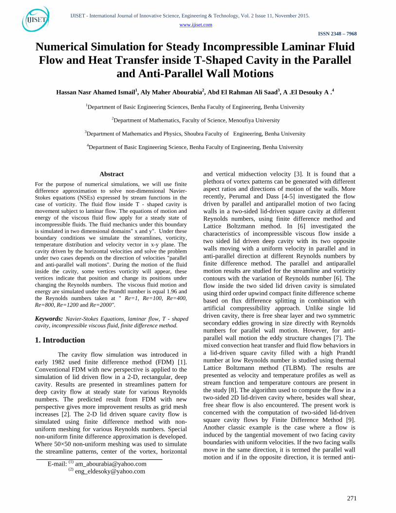
Fig. 1: The statement for

T-shaped cavity.

The Navier-Stokes equations solve under the boundary conditions which has T - shaped cavity. The cavity indicated in Fig.1 has two parts. The top part called the head and the lower part called the tail. The physical structure of the cavity itself is in dimensionless parameters and solving under aspect ratio equal to 1" α =1 and β = 1".

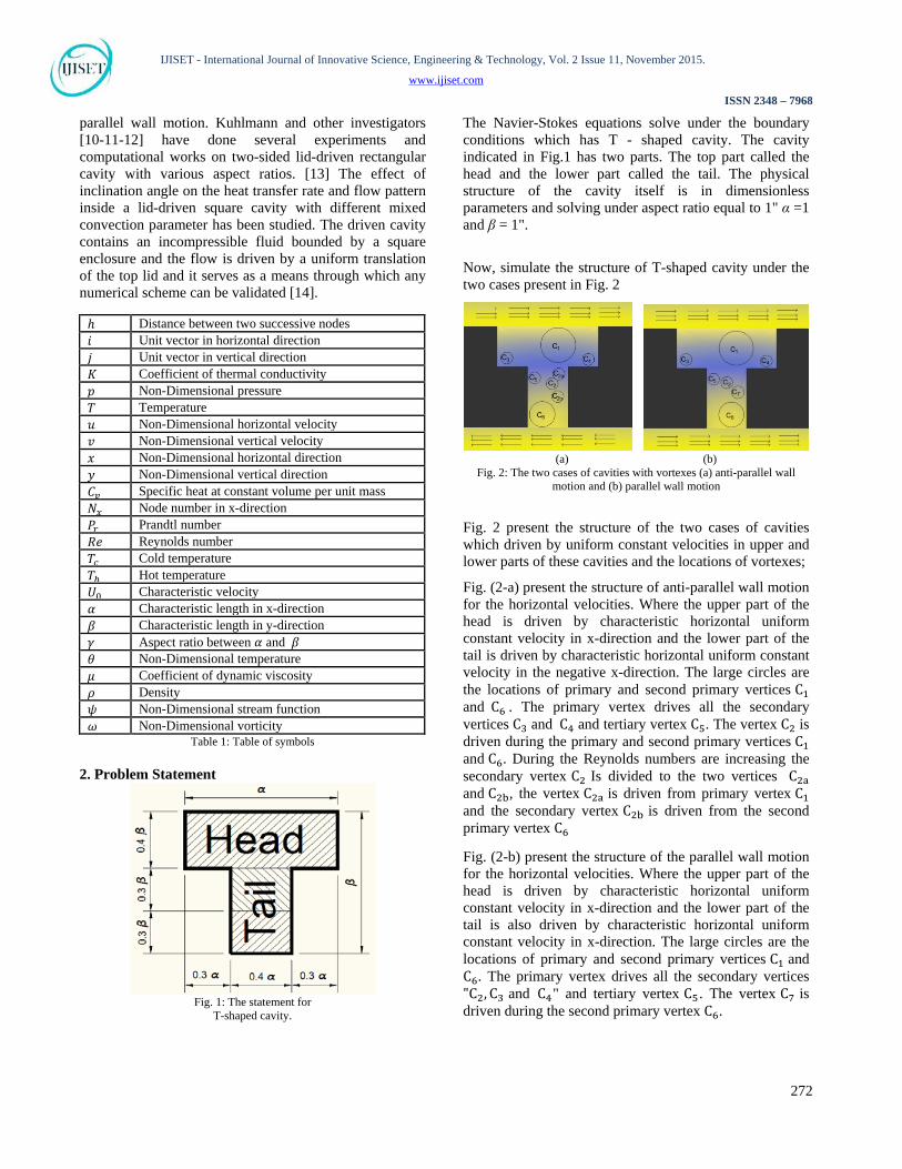
Now, simulate the structure of T-shaped cavity under the two cases present in Fig. 2

(a) (b)

Fig. 2: The two cases of cavities with vortexes (a) anti-parallel wall motion and (b) parallel wall motion

Fig. 2 present the structure of the two cases of cavities which driven by uniform constant velocities in upper and lower parts of these cavities and the locations of vortexes;

Fig. (2-a) present the structure of anti-parallel wall motion for the horizontal velocities. Where the upper part of the head is driven by characteristic horizontal uniform constant velocity in x-direction and the lower part of the tail is driven by characteristic horizontal uniform constant velocity in the negative x-direction. The large circles are the locations of primary and second primary vertices C1 and C6 . The primary vertex drives all the secondary vertices C3 and C4 and tertiary vertex C5. The vertex C2 is driven during the primary and second primary vertices C1 and C6. During the Reynolds numbers are increasing the secondary vertex C2 Is divided to the two vertices C2a and C2b, the vertex C2a is driven from primary vertex C1 and the secondary vertex C2b is driven from the second primary vertex C6

Fig. (2-b) present the structure of the parallel wall motion for the horizontal velocities. Where the upper part of the head is driven by characteristic horizontal uniform constant velocity in x-direction and the lower part of the tail is also driven by characteristic horizontal uniform constant velocity in x-direction. The large circles are the locations of primary and second primary vertices C1 and C6. The primary vertex drives all the secondary vertices "C2, C3 and C4" and tertiary vertex C5 . The vertex C7 is driven during the second primary vertex C6.

272



www.ijiset.com

ISSN 2348 – 7968

3. Governing Equations

For laminar incompressible steady state flow, the governing equations for NSEs " continuity equation, Momentum Equation in x and y direction and energy Equation"[15-16] can be written with the symbol (*) as

𝜕𝑢∗

𝜕𝑥∗+𝜕𝑣∗

𝜕𝑦∗= 0

(1)

𝜌∗ � 𝑢∗𝜕𝑢∗

𝜕𝑥∗+ 𝑣∗

𝜕𝑢∗

𝜕𝑦∗� = −

𝜕𝑝∗

𝜕𝑥∗+ 𝜇∗ �

𝜕2𝑢∗

𝜕𝑥∗2+𝜕2𝑢∗

𝜕𝑦∗2�

(2)

𝜌∗ � 𝑢∗𝜕𝑣∗

𝜕𝑥∗+ 𝑣∗

𝜕𝑣∗

𝜕𝑦∗� = −

𝜕𝑝∗

𝜕𝑦∗+ 𝜇∗ �

𝜕2𝑣∗

𝜕𝑥∗2+𝜕2𝑣∗

𝜕𝑦∗2�

(3)

𝜌∗𝐶𝑣∗ �𝑢∗𝜕𝑇∗

𝜕𝑥∗+ 𝑣∗

𝜕𝑇∗

𝜕𝑦∗� = 𝐾∗ �

𝜕2𝑇∗

𝜕𝑥∗2+𝜕2𝑇∗

𝜕𝑦∗2�

(4) Using non-dimensional parameter which used to convert Navier-Stokes equations to non-dimensional forms can written as,

𝑥 =𝑥∗

𝛼 ,𝑦 =

𝑦∗

𝛽 , 𝛾 =

𝛼𝛽

,𝑢 =𝑢∗

𝑈0 , 𝑣 =

𝑣∗

𝑈0 ,𝑝 =

𝑃∗

𝜌 𝑈02 ,

𝜃 =𝑇 − 𝑇𝑐𝑇ℎ − 𝑇𝑐

,𝜓 =𝜓∗

𝑈0 𝛼 ,𝜔 =

𝜔∗ 𝛼𝑈0

(5)

�𝜕𝑢𝜕𝑥

+ 𝛾𝜕𝑣𝜕𝑦� = 0

(6)

�𝑢𝜕𝑢𝜕𝑥

+ 𝛾𝑣𝜕𝑢𝜕𝑦� =

−𝜕𝑝𝜕𝑥

+ 1𝑅𝑒

��𝜕2𝑢𝜕𝑥2

�+ 𝛾2 �𝜕2𝑢𝜕𝑦2

��

(7)

�𝑢𝜕𝑣𝜕𝑥

+ 𝛾𝑣𝜕𝑣𝜕𝑦� = −𝛾

𝜕𝑝𝜕𝑦

+1𝑅𝑒

��𝜕2𝑣𝜕𝑥2

�+ 𝛾2 �𝜕2𝑣𝜕𝑦2

��

(8)

�𝑢𝜕𝜃𝜕𝑥

+ 𝛾𝑣𝜕𝜃𝜕𝑦� =

1𝑃𝑟𝑅𝑒

�𝜕2𝜃𝜕𝑥2

+ 𝛾2𝜕2𝜃𝜕𝑦2

�

(9) Where, Reynolds number and Prandtl number and equals

𝑅𝑒 =𝜌∗ 𝑈0 𝛼𝜇∗

, 𝑃𝑟 =𝐶𝑣∗ 𝜇∗

𝐾∗

(10) Stream function and vorticity equations during the horizontal and vertical velocities has formed [17]

𝑢∗ =𝜕𝜓∗

𝜕𝑦∗ , 𝑣∗ = −

𝜕𝜓∗

𝜕𝑥∗, 𝜔∗ =

𝜕𝑣∗

𝜕𝑥∗ −

𝜕𝑢∗

𝜕𝑦∗

(11) 23TFrom Eq. (11) and23T non-dimensional parameter (5),23T non-23Tdimensional stream function and vorticity has form.

𝑢 = 𝛾𝜕𝜓𝜕𝑦

, 𝑣 = −𝜕𝜓𝜕𝑥

, 𝜔 = −�𝜕2𝜓𝜕𝑥2

+ 𝛾2𝜕2𝜓𝜕𝑦2

�

(12) From the Eq. (7) and Eq. (12) and multiply −(𝜕/𝜕𝑦) in x-momentum, the new equation has form

−𝑢𝜕𝜕𝑦

𝜕𝑢𝜕𝑥

− 𝑣𝜕𝜕𝑦

𝜕𝑢𝜕𝑦

=𝜕𝜕𝑦

𝜕𝑝𝜕𝑥

− 1𝑅𝑒

𝜕𝜕𝑦

�𝜕2𝑢𝜕𝑥2

+𝜕2𝑢𝜕𝑦2

�

(13) From the Eq. (8) and Eq. (12) and multiply −(𝜕/𝜕𝑥) in y-momentum, the new equation has form

𝑢𝜕𝜕𝑥

𝜕𝑣𝜕𝑥

+ 𝑣𝜕𝜕𝑥

𝜕𝑣𝜕𝑦

= −𝜕𝜕𝑥

𝜕𝑝𝜕𝑦

+ 1𝑅𝑒

𝜕𝜕𝑥

�𝜕2𝑣𝜕𝑥2

+𝜕2𝑣𝜕𝑦2

�

(14) By adding Eq. (13) in Eq. (14) and from the stream function and vorticity Eq. (12), the momentum equation has form

�𝜕𝜓𝜕𝑦

𝜕𝜔𝜕𝑥

− 𝜕𝜓𝜕𝑥

𝜕𝜔𝜕𝑦� =

1𝑅𝑒

�𝜕2𝜔𝜕𝑥2

+𝜕2𝜔𝜕𝑦2

�

(15) From the Eq. (9) and from the stream function and Eq. (12), the energy equation has form.

�𝜕𝜓𝜕𝑦

𝜕𝜃𝜕𝑥

− 𝜕𝜓𝜕𝑥

𝜕𝜃𝜕𝑦� =

1𝑃𝑟 𝑅𝑒

�𝜕2𝜃𝜕𝑥2

+𝜕2𝜃𝜕𝑦2

�

(16) 4. The Boundary Condition

The boundary conditions for dimensionless stream function, horizontal velocity, vertical velocity and temperature due to the two cases indicated in Fig. 3 are as follows.

𝜓 = 0,𝑢 = 0, 𝑣 = 0 𝑎𝑛𝑑 𝜃 = 1 𝑎𝑡 𝑥 = 0.3𝛼 𝑎𝑛𝑑 0.3𝛽 ≤ 𝑦 ≤ 0.6𝛽, 𝑥 = 0.7𝛼 𝑎𝑛𝑑 0.3𝛽 ≤ 𝑦 ≤ 0.6𝛽

(17)

Fig. 3: T-shaped boundary conditions.

273



www.ijiset.com

ISSN 2348 – 7968

𝜓 = 0,𝑢 = 0, 𝑣 = 0 𝑎𝑛𝑑 𝜕𝜃𝜕𝑥

= 0 𝑎𝑡 𝑥 = 0.7𝛼 𝑎𝑛𝑑 0 ≤ 𝑦 ≤ 0.3,

𝑥 = 0.3𝛼 𝑎𝑛𝑑 0 ≤ 𝑦 ≤ 0.3𝛽 (18)

𝜓 = 0,𝑢 = 0, 𝑣 = 0 𝑎𝑛𝑑 𝜃 = 0 𝑎𝑡 𝑥 = 𝛼 𝑎𝑛𝑑 0.6 𝛽 ≤ 𝑦 ≤ 𝛽 ,

𝑥 = 0 𝑎𝑛𝑑 0.6 𝛽 ≤ 𝑦 ≤ 𝛽 (19)

𝜓 = 0,𝑢 = 0, 𝑣 = 0 𝑎𝑛𝑑 𝜕𝜃𝜕𝑦

= 0 𝑎𝑡

𝑦 = 0.6 𝛽 𝑎𝑛𝑑 0.7𝛼 ≤ 𝑥 ≤ 𝛼, 𝑦 = 0.6 𝛽 𝑎𝑛𝑑 0 ≤ 𝑥 ≤ 0.3𝛼

(20) 𝜓 = 0,𝑢 = 0, 𝑣 = 0 ,𝑎𝑛𝑑 𝜃 = 1 𝑎𝑡 𝑦 = 𝛽 𝑎𝑛𝑑 0 ≤ 𝑥 ≤ 𝛼

(21) 𝜓 = 0, 𝑣 = 0 ,𝑎𝑛𝑑 𝜃 = 1 𝑎𝑡 𝑦 = 0 𝑎𝑛𝑑 0.3𝛼 ≤ 𝑥 ≤ 0.7𝛼 and the horizontal velocity for anti-parallel wall motion and parallel wall motion are equal to u = −1 and u = 1 respectively. 5. Two Dimensional Grid Generation for the

Two Cases

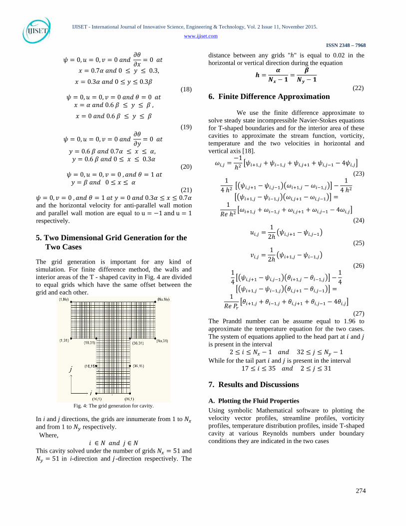
The grid generation is important for any kind of simulation. For finite difference method, the walls and interior areas of the T - shaped cavity in Fig. 4 are divided to equal grids which have the same offset between the grid and each other.

Fig. 4: The grid generation for cavity.

In i and j directions, the grids are innumerate from 1 to 𝑁𝑥 and from 1 to 𝑁𝑦 respectively. Where,

𝑖 ∈ 𝑁 𝑎𝑛𝑑 𝑗 ∈ 𝑁 This cavity solved under the number of grids 𝑁𝑥 = 51 and 𝑁𝑦 = 51 in i-direction and 𝑗-direction respectively. The

distance between any grids "h" is equal to 0.02 in the horizontal or vertical direction during the equation

𝒉 =𝜶

𝑵𝒙 − 𝟏=

𝜷𝑵𝒚 − 𝟏

(22) 6. Finite Difference Approximation

We use the finite difference approximate to solve steady state incompressible Navier-Stokes equations for T-shaped boundaries and for the interior area of these cavities to approximate the stream function, vorticity, temperature and the two velocities in horizontal and vertical axis [18].

𝜔𝑖,𝑗 =−1ℎ2

�𝜓𝑖+1,𝑗 + 𝜓𝑖−1,𝑗 + 𝜓𝑖,𝑗+1 + 𝜓𝑖,𝑗−1 − 4𝜓𝑖,𝑗� (23)

14 ℎ2

��𝜓𝑖,𝑗+1 − 𝜓𝑖,𝑗−1��𝜔𝑖+1,𝑗 − 𝜔𝑖−1,𝑗�� −1

4 ℎ2

��𝜓𝑖+1,𝑗 − 𝜓𝑖−1,𝑗��𝜔𝑖,𝑗+1 − 𝜔𝑖,𝑗−1�� = 1

𝑅𝑒 ℎ2�𝜔𝑖+1,𝑗 + 𝜔𝑖−1,𝑗 + 𝜔𝑖,𝑗+1 + 𝜔𝑖,𝑗−1 − 4𝜔𝑖,𝑗�

(24)

𝑢𝑖,𝑗 =12ℎ

�𝜓𝑖,𝑗+1 − 𝜓𝑖,𝑗−1� (25)

𝑣𝑖,𝑗 =12ℎ

�𝜓𝑖+1,𝑗 − 𝜓𝑖−1,𝑗� (26)

14��𝜓𝑖,𝑗+1 − 𝜓𝑖,𝑗−1��𝜃𝑖+1,𝑗 − 𝜃𝑖−1,𝑗�� −

14

��𝜓𝑖+1,𝑗 − 𝜓𝑖−1,𝑗��𝜃𝑖,𝑗+1 − 𝜃𝑖,𝑗−1�� = 1

𝑅𝑒 𝑃𝑟�𝜃𝑖+1,𝑗 + 𝜃𝑖−1,𝑗 + 𝜃𝑖,𝑗+1 + 𝜃𝑖,𝑗−1 − 4𝜃𝑖,𝑗�

(27) The Prandtl number can be assume equal to 1.96 to approximate the temperature equation for the two cases. The system of equations applied to the head part at 𝑖 and 𝑗 is present in the interval

2 ≤ 𝑖 ≤ 𝑁𝑥 − 1 𝑎𝑛𝑑 32 ≤ 𝑗 ≤ 𝑁𝑦 − 1 While for the tail part 𝑖 and 𝑗 is present in the interval

17 ≤ 𝑖 ≤ 35 𝑎𝑛𝑑 2 ≤ 𝑗 ≤ 31

7. Results and Discussions

A. Plotting the Fluid Properties Using symbolic Mathematical software to plotting the velocity vector profiles, streamline profiles, vorticity profiles, temperature distribution profiles, inside T-shaped cavity at various Reynolds numbers under boundary conditions they are indicated in the two cases

274



www.ijiset.com

ISSN 2348 – 7968

(a) (b)

(c) (d)

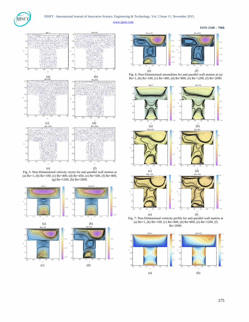
(e) (f) Fig. 5: Non-Dimensional velocity vector for anti-parallel wall motion at (a) Re=1, (b) Re=100, (c) Re=400, (d) Re=450, (e) Re=500, (f) Re=800,

(g) Re=1200, (h) Re=2000.

(a) (b)

(c) (d)

(e) (f) Fig. 6: Non-Dimensional streamlines for anti-parallel wall motion at (a) Re=1, (b) Re=100, (c) Re=400, (d) Re=800, (e) Re=1200, (f) Re=2000.

(a) (b)

(c) (d)

(e) (f) Fig. 7: Non-Dimensional vorticity profile for anti-parallel wall motion at

(a) Re=1, (b) Re=100, (c) Re=400, (d) Re=800, (e) Re=1200, (f) Re=2000.

(a) (b)

275



www.ijiset.com

ISSN 2348 – 7968

(c) (d)

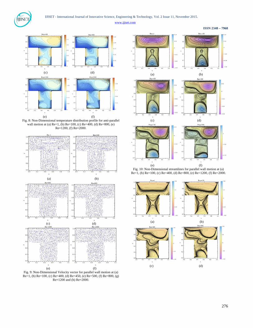
(e) (f) Fig. 8: Non-Dimensional temperature distribution profile for anti-parallel

wall motion at (a) Re=1, (b) Re=100, (c) Re=400, (d) Re=800, (e) Re=1200, (f) Re=2000.

(a) (b)

(c) (d)

(e) (f) Fig. 9: Non-Dimensional Velocity vector for parallel wall motion at (a)

Re=1, (b) Re=100, (c) Re=400, (d) Re=450, (e) Re=500, (f) Re=800, (g) Re=1200 and (h) Re=2000.

(a) (b)

(c) (d)

(e) (f)

Fig. 10: Non-Dimensional streamlines for parallel wall motion at (a) Re=1, (b) Re=100, (c) Re=400, (d) Re=800, (e) Re=1200, (f) Re=2000.

(a) (b)

(c) (d)

276



www.ijiset.com

ISSN 2348 – 7968

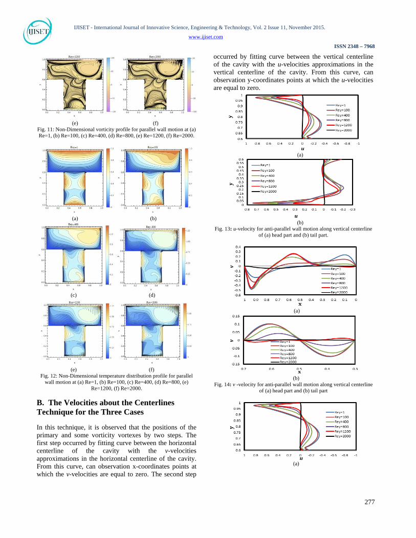
(e) (f) Fig. 11: Non-Dimensional vorticity profile for parallel wall motion at (a) Re=1, (b) Re=100, (c) Re=400, (d) Re=800, (e) Re=1200, (f) Re=2000.

(a) (b)

(c) (d)

(e) (f)

Fig. 12: Non-Dimensional temperature distribution profile for parallel wall motion at (a) Re=1, (b) Re=100, (c) Re=400, (d) Re=800, (e)

Re=1200, (f) Re=2000.

B. The Velocities about the Centerlines Technique for the Three Cases

In this technique, it is observed that the positions of the primary and some vorticity vortexes by two steps. The first step occurred by fitting curve between the horizontal centerline of the cavity with the v-velocities approximations in the horizontal centerline of the cavity. From this curve, can observation x-coordinates points at which the v-velocities are equal to zero. The second step

occurred by fitting curve between the vertical centerline of the cavity with the u-velocities approximations in the vertical centerline of the cavity. From this curve, can observation y-coordinates points at which the u-velocities are equal to zero.

(a)

(b)

Fig. 13: u-velocity for anti-parallel wall motion along vertical centerline of (a) head part and (b) tail part.

(a)

(b)

Fig. 14: v -velocity for anti-parallel wall motion along vertical centerline of (a) head part and (b) tail part

(a)

277



www.ijiset.com

ISSN 2348 – 7968

(b)

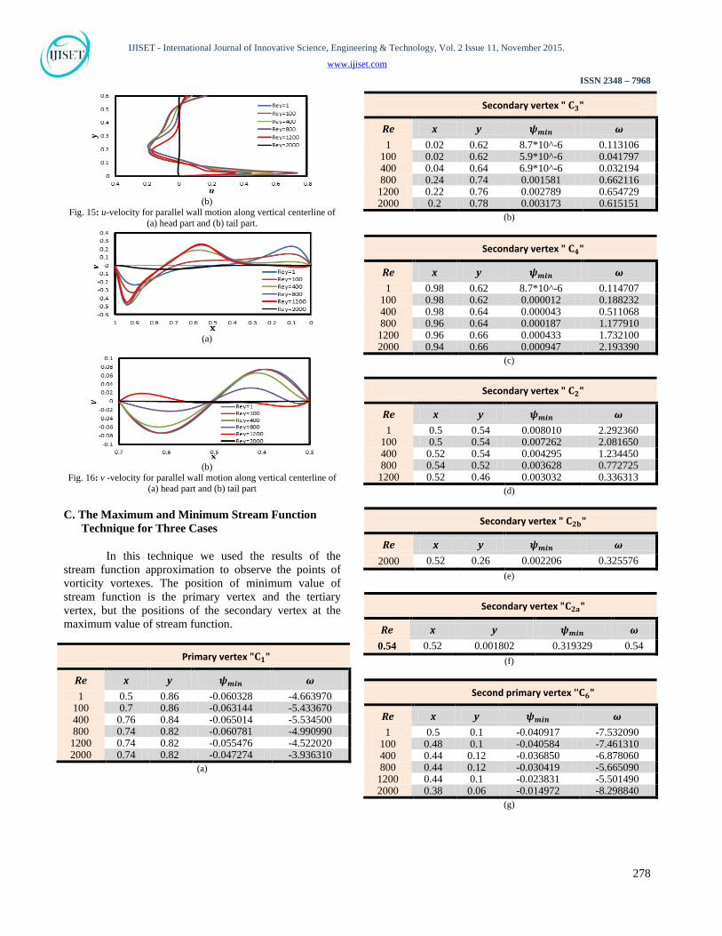
Fig. 15: u-velocity for parallel wall motion along vertical centerline of (a) head part and (b) tail part.

(a)

(b)

Fig. 16: v -velocity for parallel wall motion along vertical centerline of (a) head part and (b) tail part

C. The Maximum and Minimum Stream Function Technique for Three Cases

In this technique we used the results of the stream function approximation to observe the points of vorticity vortexes. The position of minimum value of stream function is the primary vertex and the tertiary vertex, but the positions of the secondary vertex at the maximum value of stream function.

Primary vertex "𝐂𝟏"

Re x y 𝝍𝒎𝒊𝒏 ω 1 0.5 0.86 -0.060328 -4.663970

100 0.7 0.86 -0.063144 -5.433670 400 0.76 0.84 -0.065014 -5.534500 800 0.74 0.82 -0.060781 -4.990990

1200 0.74 0.82 -0.055476 -4.522020 2000 0.74 0.82 -0.047274 -3.936310

(a)

Secondary vertex " 𝐂𝟑"

Re x y 𝝍𝒎𝒊𝒏 ω 1 0.02 0.62 8.7*10^-6 0.113106

100 0.02 0.62 5.9*10^-6 0.041797 400 0.04 0.64 6.9*10^-6 0.032194 800 0.24 0.74 0.001581 0.662116 1200 0.22 0.76 0.002789 0.654729 2000 0.2 0.78 0.003173 0.615151

(b)

Secondary vertex " 𝐂𝟒"

Re x y 𝝍𝒎𝒊𝒏 ω 1 0.98 0.62 8.7*10^-6 0.114707

100 0.98 0.62 0.000012 0.188232 400 0.98 0.64 0.000043 0.511068 800 0.96 0.64 0.000187 1.177910 1200 0.96 0.66 0.000433 1.732100 2000 0.94 0.66 0.000947 2.193390

(c)

Secondary vertex " 𝐂𝟐"

Re x y 𝝍𝒎𝒊𝒏 ω 1 0.5 0.54 0.008010 2.292360

100 0.5 0.54 0.007262 2.081650 400 0.52 0.54 0.004295 1.234450 800 0.54 0.52 0.003628 0.772725

1200 0.52 0.46 0.003032 0.336313 (d)

Secondary vertex " 𝐂𝟐𝐛"

Re x y 𝝍𝒎𝒊𝒏 ω 2000 0.52 0.26 0.002206 0.325576

(e)

Secondary vertex "𝐂𝟐𝐚"

Re x y 𝝍𝒎𝒊𝒏 ω 0.54 0.52 0.001802 0.319329 0.54

(f)

Second primary vertex ''𝐂𝟔"

Re x y 𝝍𝒎𝒊𝒏 ω 1 0.5 0.1 -0.040917 -7.532090

100 0.48 0.1 -0.040584 -7.461310 400 0.44 0.12 -0.036850 -6.878060 800 0.44 0.12 -0.030419 -5.665090

1200 0.44 0.1 -0.023831 -5.501490 2000 0.38 0.06 -0.014972 -8.298840

(g)

278



www.ijiset.com

ISSN 2348 – 7968

Tertiary vertex ''𝐂𝟓"

Re x y 𝝍𝒎𝒊𝒏 ω 0.54 0.32 0.58 -0.000007 -0.097117

Table 2: Simulation of vertices for anti-parallel wall motion under the various of Reynolds numbers for (a) vertex '' C1'', (b) vertex '' C3'', (c)

vertex '' C4'', (d) vertex''C2'', (e) vertex '' C2b'', (f) vertex '' C2a'', (g) vertex ''C6'' and (h) vertex ''C5''

Primary vertex "𝐂𝟏"

Re x y 𝝍𝒎𝒊𝒏 ω 1 0.5 0.86 -0.060328 -4.663970

100 0.7 0.86 -0.063144 -5.433670 400 0.76 0.84 -0.065014 -5.534500 800 0.74 0.82 -0.060781 -4.990990

1200 0.74 0.82 -0.055476 -4.522020 2000 0.74 0.82 -0.047274 -3.936310

(a)

Secondary vertex "𝐂𝟑"

Re x y 𝝍𝒎𝒊𝒏 ω 1 0.02 0.62 8.72*10^-6 0.113106

100 0.02 0.62 5.93*10^-6 0.041797 400 0.04 0.64 6.97*10^-6 0.032194 800 0.24 0.74 0.001581 0.662116

1200 0.22 0.76 0.002789 0.654729 2000 0.2 0.78 0.003173 0.615151

(b)

Secondary vertex " 𝐂𝟒"

Re x y 𝝍𝒎𝒊𝒏 ω 1 0.98 0.62 8.74*10^-6 0.114707

100 0.98 0.62 0.000012 0.188232 400 0.98 0.64 0.000036 0.177142 800 0.96 0.64 0.000187 1.177910 1200 0.96 0.66 0.000433 1.732100 2000 0.94 0.66 0.000947 2.193390

(c)

Second primary vertex ''𝐂𝟔"

Re x y 𝝍𝒎𝒊𝒏 ω 1 0.5 0.1 0.041065 7.494580

100 0.52 0.1 0.040703 7.405220 400 0.56 0.12 0.037060 6.754100 800 0.56 0.12 0.030533 5.480450

1200 0.56 0.1 0.023868 5.417130 2000 0.64 0.06 0.004240 0.166997

(d)

Secondary vertex " 𝐂𝟐"

Re x y 𝝍𝒎𝒊𝒏 ω 1 0.5 0.5 0.009629 1.487750

100 0.5 0.5 0.008811 1.311510 400 0.5 0.52 0.004275 0.746777 800 0.56 0.56 0.002573 1.186520 1200 0.58 0.56 0.001997 1.088830 2000 0.56 0.56 0.001666 0.790605

(e)

Tertiary vertex " 𝐂𝟕"

Re x y 𝝍𝒎𝒊𝒏 ω 400 0.68 0.36 -0.000018 -0.260378 800 0.6 0.36 -0.000422 -0.759700

1200 0.48 0.34 -0.001625 -0.616726 2000 0.46 0.24 -0.001996 -0.443466

(f)

Tertiary vertex '' 𝐂𝟓''

Re x y 𝝍𝒎𝒊𝒏 ω 800 0.6 0.36 -0.000422 -0.759700

1200 0.48 0.34 -0.001625 -0.616726 2000 0.46 0.24 -0.001996 -0.443466

(g)

Table 3: Simulation of vertices for parallel wall motion under the various of Reynolds numbers for (a) vertex '' C1'', (b) vertex

'' C3'', (c) vertex '' C4'', (d) vertex '' C6'', (e) vertex '' C2'', (f) vertex '' C7'' and (g) vertex '' C5''.

Table (2) present Simulation of vertices for anti-parallel wall motion under the various of Reynolds numbers and Show its locations and the value of the stream function and vorticity. For vertex C1 , C6 and C5 , has a negative sign of the stream function and vorticity for any Reynolds number, this means that the vortices rotating clockwise. For the vertices '' C3 '', '' C4 '', C2b , C2a and '' C2 '', has a positive sign of the stream function and vorticity for any Reynolds number, this means that the vortices rotating counterclockwise.

Table (3) present Simulation of vertices for parallel wall motion under the various of Reynolds numbers and Show its locations and the value of the stream function and vorticity. For vertex C1 , C7 and C5, has a negative sign of the stream function and vorticity for any Reynolds number, this means that the vortices rotating clockwise. For the vertices '' C3'', '' C4'', C6 and '' C2'', has a positive sign of the stream function and vorticity for any Reynolds number, this means that the vortices rotating counterclockwise.

279



www.ijiset.com

ISSN 2348 – 7968

8. Conclusions

The viscous fluid flow and energy inside T-shaped cavity was simulated for different Reynolds numbers and Prandtl number is equal 1.96. Using the finite difference method to solve Navier-Stokes equations which for the stream functions and vorticity to simulate the fluid mechanics. The equations of motion of the viscous fluid flow subject to laminar flow are applied in steady state for incompressible fluid with the boundary conditions. We simulate the streamline, vorticity, temperature distribution and velocities in x-y plane. The horizontal velocities in the parallel and anti-parallel wall motion drive the cavity. During these motions, some vertices vorticity has appeared and observed that position and change its positions under changed the Reynolds number. References

[1] K.N. Ghia and C.T. Shin, "High-Resolutions for incompressible flow using the Navier–Stokes equations and a multigrid method", Journal of Computational Physics, Vol. 48, PP. 367-411, (1982)

[2] M.S. Idris and N.M.N.M. Ammar, "2-D Deep Cavity Flow, Lid Driven Using Conventional Method With New Perspective", National Conference in Mechanical Engineering Research and Postgraduate Studies, Faculty of Mechanical Engineering, UMP Pekan, Kuantan, Pahang, pp. 550-558, (2010).

[3] M.S.Idris and C.S.N. Azwadi,"Numerical Investigation of 2-D Lid Driven Cavity Flow Emphasizing Finite Difference Method of Non Uniform Meshing", National Conference in Mechanical Engineering Research and Postgraduate Students, FKM Conference Hall, UMP, Kuantan, Pahang, Malaysia, pp. 91-98, (2010).

[4] Perumal, Anoop K.Dass,"Simulation of incompressible flows in two-sided lid-driven square cavities. Part I – FDM", CFD Letters, Issue 1, Vol. 2(1), pp. 13-24, (2010).

[5] Perumal, Anoop K.Dass,"Simulation of incompressible flows in two-sided lid-driven square cavities, Part II – LBM", CFD Letters, Issue 1, Vol. 2(1), pp. 25-38, (2010).

[6] Perumal, "Simulation of Flow in Two-Slid Lid Driven Deep Cavities by Finite Difference Method", Journal of applied science in the thermodynamics and fluid mechanics, Vol. 6(1), (2012)

[7] A. Munir, M. Rizwan, M. Khan and A.Shah, "Simulation of Incompressible Flow in Two Sided Lid

Driven Cavity using Upwind Compact Scheme", CFD Letters, Vol. 5(3), pp. 57-66, (2013).

[8] M. A. Taher, S. C. Saha, Y. W. Lee, H. D. Kim, "Numerical Study of Lid-Driven Square Cavity with Heat Generation Using LBM", American Journal of Fluid Dynamics, Vol. 3(2), PP. 40-47, (2013).

[9] N. Kumar, J.C. Kalita and A.K. Dass, "Computation of Two-Sided Lid-Driven Cavity Flow", Conference on Computational Mechanics and Simulation, ICCMS, IIT Guwahati, India, (2006).

[10] H.C. Kuhlmann, M. Wanschura, and H.J. Rath, "Flow in two-sided lid-driven cavities: no uniqueness, instability, and cellular structures", Journal of Computational Physics, vol. 336, PP. 267-299, (1997).

[11] S. Albensoeder, H.C. Kuhlmann, and H.C. Rath, "Multiplicity of Steady Two Dimensional Flows in Two-sided Lid-Driven Cavities", Theoretical Computational Fluid Dynamics, Vol. 14: PP. 223-241, (2001).

[12] C.H .Blohm, and H.C. Kuhlmann, "The two-sided lid-driven cavity: experiments on stationary and time-dependent flows", Journal of Fluid Mechanics, Vol. 450, PP. 67-95, (2002).

[13] A. A.R. Darzi, M. Farhadi, K. Sedighi, E. Fattahi and H. Nemati, "Mixed convection simulation on inclined lid driven cavity using Lattice Boltzmann method", Transactions of Mechanical Engineering, , Vol. 35, PP. 73-83, (2011).

[14] R. Begum and A. M. Basit, "Lattice Boltzmann Method and its Applications to Fluid Flow Problems", European Journal of Scientific Research, ISSN 1450-216X, Vol. 22(2), PP. 216-23, (2008).

[15] L. Currie, "Fundamental Mechanics of Fluids", university of Jodhpur (India), third Edition, (1977).

[16] J. L. Bansal, "Viscous Fluid Dynamics", university of toronto (Canada), (1977).

[17] Batchelor, George K, "An Introduction to Fluid Dynamics", Cambridge University Press, (1967)

[18] H. N.A. Ismail, "Selected Topics of Numerical Analysis and Scientific Computation", El mostapha Publishing house, Cairo, (2015)

280


https://en.wikipedia.org/wiki/George_Batchelor

Numerical Simulation for Steady Incompressible Laminar...

Documents

Transcript of Numerical Simulation for Steady Incompressible Laminar...