Some Investigation Of Incompressible Inviscid Steady Flow ... · Some Investigation Of...

Some Investigation Of Incompressible Inviscid Steady Flow In Engineering

Systems: A Case Study Of The Bernoulli’s Equation With Its Application To

Leakage In Tanks Mutua, N. M 1, Wanyama, D. S 2, Kiogora, P. R 3

1Mathematics and Informatics, Taita Taveta University College, Voi, 80300, Kenya 2Mathematics and Informatics, Taita Taveta University College, Voi, 80300, Kenya

3Pure and Applied Mathematics, Jomo Kenyatta University of Agriculture and Technology, Nairobi,

62000-00200, Kenya

780

International Journal of Engineering Research & Technology (IJERT)

Vol. 2 Issue 8, August - 2013

IJERT

IJERT

ISSN: 2278-0181

www.ijert.orgIJERTV2IS80178

Abstract

During fluid spill incidents involving damaged

tanks, the amount of the product released may be

uncertain. Many accidents occur under adverse

conditions, so determining the volume lost by

sounding the tanks may not be practical. In the first

few hours, initial volume estimates often are based

on visual observations of the resulting levels, a

notorious unreliable approach. This study has

described a computer based model by Bernoulli’s

equation that will help in responding to leakages in

tanks.

1. Introduction Fluid storage tanks can be damaged in the

course of their life and a substantial amount of the

fluid lost through leakage. There is need therefore

to calculate the rate at which the tank leaks in order

to adequately respond to the situation. The volume

of a fluid escaping through a hole in the side of a

storage tank has been calculated by the Bernoulli’s

equation which has been adapted to a streamline

from the surface to the orifice.

1.1 Objectives

The objectives of the study are:

i. To determine the velocity of the fluid

through the opening in the tank.

ii. To determine the volume flow rate

through the opening.

iii. To determine the mass flow rate through

the opening.

1.2 Justification

Fluid storage tanks e.g. water reservoirs &

petroleum oil tanks are commonly used in our

society today. This storage tanks are prone to

accidents which when not adequately responded to,

great losses will be incurred in terms of money and

also pollution to the environment. The volume of a

fluid escaping through a hole in the side of a

storage tank is calculated by the Bernoulli’s

equation calculator the results of which are useful

for developing the intuitively skills of responders

and planners in spill releases.

1.3 Literature Review

Castelli and Tonicelli (1600) were first to state

that the velocity through a hole in a tank varies as

square root of water level above the hole. They also

stated that the volume flow rate through the hole is

proportional to the open area. It was almost another

century later that a Swiss physicist Daniel

Bernoulli (1738) developed an equation that

defined the relationship of forces due to the line

pressure to energy of the moving fluid and earth’s

gravitational forces on the fluid. Bernoulli’s

theorem has since been the basis for flow equation

of flow meters that expresses flow rate to

differential pressure between two reference points.

Since the differential pressure can also be

expressed in terms of height or head of liquid

above a reference plane. An Italian scientist,

Giovanni Venturi (1797), demonstrated that the

differential pressure across an orifice plate is a

square root function of the flow rate through the

pipe. This is the first known use of an orifice for

measuring flow rate through a pipe. Prior to

Giovanni’s experimental demonstration, the only

accepted flow measurement method was by filling

a bucket of known volume and counting the

number of buckets being filled. The use of orifice

plates as a continuous flow rate measuring device

has a history of over two hundred years.

Subsequent experiments, Industry standards online

in their demonstration showed that liquids flowing

from a tank through an orifice close to the bottom

are governed by the Bernoulli’s equation which can

be adapted to a streamline from the surface to the

orifice. They evaluated three cases whereby in a

vented tank, the velocity out from the tank is equal

to the speed of a freely body falling the distance h -also known as Torricelli’s Theorem. In a

pressurized tank, the tank is pressurized so that

product of gravity and height gh

is much lesser

than the pressure difference divided by the density.

The velocity out from the tank depends mostly on

the pressure difference. Due to friction the real

velocity will be somewhat lower than these

theoretic examples. On leaking tank models, a

recent literature review reveals numerous papers

describing formulas for calculating discharges of

non-volatile liquids from tanks Burgreen (1960);

Dodge and Bowls(1982); Elder and Sommerfeld

(1974); Fthenakis and Rohatgi (1999); Hart and

Sommerfeld (1993); Koehler(1984); Lee and

Sommerfeld (1984); Shoaei and Sommerfeld

(1984); Simecek-Beatty et al. There are also

computer models available in ship salvage

operations. These types of models estimate the

hydrostatic, stability, and strength characteristic of

a vessel using limited data. The models require the

user to have an understanding of basic salvage and

architectural principles, skills not typical of most

spill responders or contingency planners. A simple

computer model, requiring input of readily

available data, would be useful for developing the

intuitively skills of responders and planners in spill

releases. Mathematical formulas have been

developed to accurately describe releases for light

and heavy oils. Dodge and Bowles (1982);

Fthenakis and Rohatgi (1999); Simecek-Beatty et

al. (1997). However, whether any of these models

can describe the unique characteristics of fluids

781



IJERT

IJERT

ISSN: 2278-0181


accurately is not known. Observational data of

these types of releases are needed to test existing

models, and probably modify them in the case of a

given fluid. J. Irrig and Drain. Engrg (August 2010)

carried out experiments under different orifice

diameters and water heads. The dependence of the

discharge coefficient on the orifice diameter and

water head was analysed, and then an empirical

relation was developed by using a dimensional

analysis and a regression analysis. The results

showed that the larger orifice diameter or higher

water head have a smaller discharge coefficient and

the orifice diameter plays more significant

influence on the discharge coefficient than the

water head does. The discharge coefficient of water

flow through a bottom orifice is larger than that

through a sidewall orifice under the similar

conditions of the water head, orifice diameter, and

hopper size.

In this research work a simple computer model,

based on Bernoulli’s equation requiring input of

readily available data, is used to investigate leakage

from vessels or tanks: the case of two pipeline

companies (Oil refineries and Kenya pipeline co.)

in the Coast province of Kenya. The results are of

vital importance in responding to leakages to

minimize losses.

This template, created in MS Word 2003 and

saved as “Word 2003 – doc” for the PC, provides

authors with most of the formatting specifications

needed for preparing electronic versions of their

papers. All standard paper components have been

specified for three reasons: 1) ease of use when

formatting individual papers, 2) automatic

compliance to electronic requirements that

facilitate the concurrent or later production of

electronic products, and 3) Margins, column

widths, line spacing, and type styles are built-in;

examples of the type styles are provided throughout

this document. Some components, such as multi-

levelled equations, graphics, and tables are not

prescribed, although the various table text styles are

provided. The formatter will need to create these

components, incorporating the applicable criteria

that follow. Use the styles, fonts and point sizes as

defined in this template, but do not change or

redefine them in any way as this will lead to

unpredictable results. You will not need to

remember shortcut keys. Just a mouse-click at one

of the menu options will give you the style that you

want.

2. Governing Equations

2. 1 Overview

The equations governing the flow of an

incompressible inviscid steady fluid through an

orifice in a tank are presented in this chapter. This

chapter first considers the assumptions and

approximations made in this particular flow

problem and the consequences arising due to these

assumptions. The conservation equations of mass,

momentum, energy to be considered in the study

are stated, Bernoulli’s equation derived followed

by a model description of the fluid flow under

consideration.

Finally a simple computer model, requiring input

of readily available data is built which will be used

in investigating flow rate in chapter three.

2.2 Assumptions and approximations

The following assumptions have been made.

1. Fluid is incompressible i.e. density is a

constant and 0

t

2. Fluid is inviscid i.e. the fluid under

investigation is not viscous.

3. Flow is steady in that is if F is a flow

variable defined as ),,( tyxF then

0

t

F

4. Flow is along a streamline.

5. The fluid speed is sufficiently subsonic

3.0machV

6. Discharge coefficient C value is typically

between 0.90 and 0.98.

2.3 Consequences as a result of the assumptions

The fact that as the water issues out of the orifice

from the tank, the level in it changes and the flow

is, strictly speaking, not steady. However,

if 21 AA , this effect (as measured by the ratio of

the rate of change in the level and velocity 2V ), is

so small that the error made is insignificant.

The assumption of incompressibity would not

hold at varying temperatures for a fluid like water

which has differing densities at different

temperatures. However this is taken care of by our

model which allows the user to enter determined

values of densities at various temperatures.

2.4 The Governing Equations

2.4.1 Equation of conservation of mass

Consider the fluid element of volume v fixed in

space surrounded by a smooth surface S . If the

density of the fluid is and dv is the volume

element of v at a point p in v , then the total mass

of the fluid in v is given by

782



IJERT

IJERT

ISSN: 2278-0181


v

dv

1

We let s be an element of the surface S .

Then if the fluid flows outwards through s , and

after time t this fluid is displaced a distance

equal to x . Then the rate at which mass is leaving

the volume element is given by

t

xLims

t

xsLim

tt

00 2

t

x

is taken to be speed.

If n̂ is the unit normal vector to s , then

fnt

xLim

t

ˆ

0

( f

denotes

velocity).

Thus

nfst

xsLim

tˆ.

0

3

This gives the rate of mass flux flowing out of v .

From 3 , the total mass flux flowing out of v

through S is given by

s

snf ˆ

4

From Gauss theorem, equation 4 can be

written as

vs

dvfsnf

ˆ 5

From equation 1 the rate at which the mass is

changing in volume v is

v

dvt

6

Applying the law of conservation of mass, we

have,

vvv

dvt

dvt

dvf

Or

0

v v

dvt

dvf

v

dvt

f 0

7

Since v is an arbitrary volume, then for equation

7 to hold, we have

0

tf

8

And this is the general equation of mass

conservation.

If is a constant, then equation 8 becomes

0f

9

This is the equation of continuity of an

incompressible fluid flow.

On the other hand, if the flow is steady i.e. the

flow variables don’t depend on time, and then

equation 8 reduces to

0 f

10

This is the equation of continuity of a steady

fluid flow.

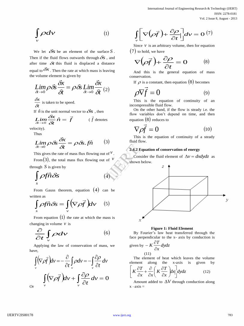
2.4.2 Equation of conservation of energy

Consider the fluid element of dxdydzv as

shown below.

Figure 1: Fluid Element

By Fourier’s law heat transferred through the

face perpendicular to the x- axis by conduction is

given by dydzx

TK

(11)

The element of heat which leaves the volume

element along the x-axis is given by

dydzdxx

TK

xx

TK

(12)

Amount added to V through conduction along

x –axis =

783



IJERT

IJERT

ISSN: 2278-0181


dxdzdyx

TK

x

dzdydxx

TK

xx

TK

x

TK

(13)

Similarly the amount added to v along the y-

axis and z- axis through conduction is

dxdydzx

TK

y

and dxdydz

x

TK

z

.

Total heat added to v by conduction

dxdydzz

TK

zy

TK

yx

TK

xt

Q

(14)

(Q is purely due to heat conduction)

If we let e be the internal energy per unit mass,

then total internal energy of the fluid

element v i.e. edxdydzev .

(15)

From this we have

dxdydzdt

de

dt

dev

dt

de (16)

So

dt

dwdxdydz

dt

de

dxdydzz

TK

zy

TK

yx

TK

x

or

dt

dw

vdt

de

z

TK

zy

TK

yx

TK

x

1

(17)

If the fluid is incompressible then 0dw for

incompressible fluids equation (17) reduces to

dt

de

z

TK

zy

TK

yx

TK

x

(18)

Adding heat generation by frictional force to

equation (18) we have,

dt

de

z

TK

zy

TK

yx

TK

x (19)

where is known as the dissipation function

given by

22

2

2222

3

2

2

z

w

y

v

x

u

y

w

z

v

x

w

z

u

x

v

y

u

z

w

y

v

x

u

(20)

(19) is the general equation of energy of the fluid

flow whose velocity components are vu, and w if

is as defined by (20)

It is noted that if the fluid is incompressible K =

a constant and the internal energy E is a function of

t alone, then equation (19) reduces to

dt

Tdf

z

T

y

T

x

TK

2

2

2

2

2

2

(T=temperature)

dt

TdfTK

)(2 (21)

If e is a function of T alone then

TCTfTCe VV (22)

substituting this in (21) we have

t

TCTK V

2 (23)

(23) is the equation of energy of a non- viscous

incompressible fluid with constant coefficient of

conductivity.

2.43 Equation of motion for compressible fluids

Consider a control volume ABCD (of unit depth)

in a 2-D flow field with its centre located at (x, y).

If the state of stress at (x, y) in this 2-D flow field is

represented by xx , yy , xy and yx , then the

surface forces on the four faces of the CV can be

written in terms of these stresses and their

derivatives using Taylor series. A few of these are

shown in the figure below.

784



IJERT

IJERT

ISSN: 2278-0181


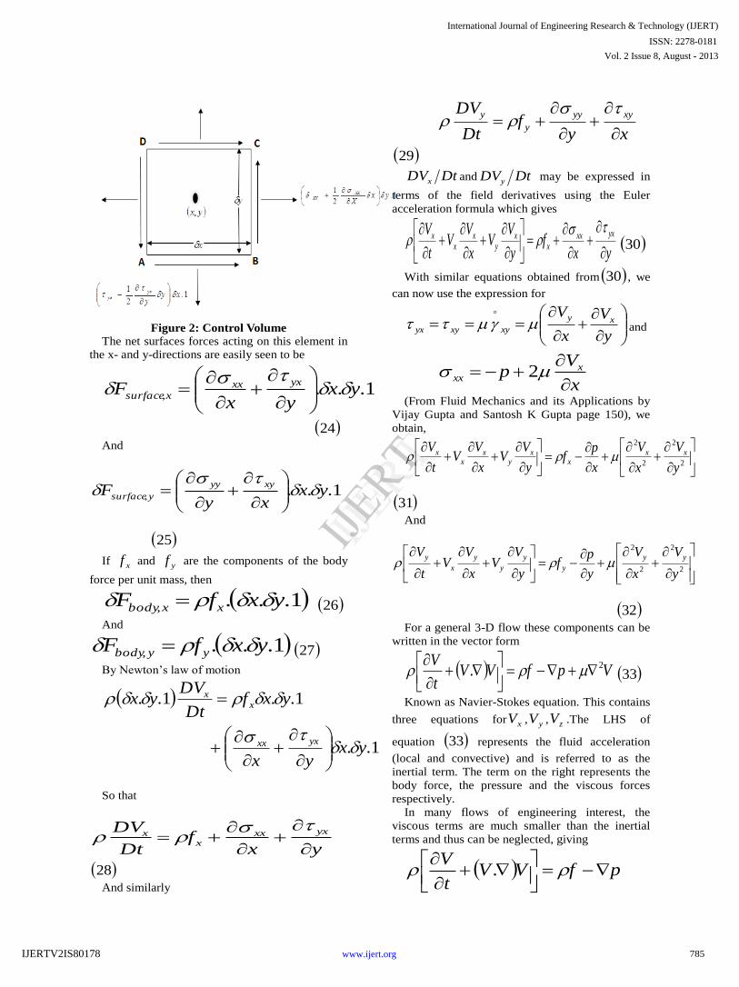
Figure 2: Control Volume

The net surfaces forces acting on this element in

the x- and y-directions are easily seen to be

1..., yxyx

Fyxxx

xsurface

24

And

1..., yxxy

Fxyyy

ysurface

25

If xf and yf are the components of the body

force per unit mass, then

1..., yxfF xxbody 26

And

1..., yxfF yybody 27

By Newton’s law of motion

1..

1..1..

yxyx

yxfDt

DVyx

yxxx

xx

So that

yxf

Dt

DV yxxxx

x

28

And similarly

xy

fDt

DV xyyy

y

y

29

DtDVx and DtDVy may be expressed in

terms of the field derivatives using the Euler

acceleration formula which gives

yxf

y

VV

x

VV

t

V yxxxx

xy

xx

x

30

With similar equations obtained from 30 , we

can now use the expression for

y

V

x

Vxy

xyxyyx

and

x

Vp x

xx

2

(From Fluid Mechanics and its Applications by

Vijay Gupta and Santosh K Gupta page 150), we

obtain,

2

2

2

2

y

V

x

V

x

pf

y

VV

x

VV

t

V xxx

xy

xx

x

31

And

2

2

2

2

y

V

x

V

y

pf

y

VV

x

VV

t

V yy

y

y

y

y

x

y

32

For a general 3-D flow these components can be

written in the vector form

VpfVVt

V 2.

33

Known as Navier-Stokes equation. This contains

three equations for xV , yV , zV .The LHS of

equation 33 represents the fluid acceleration

(local and convective) and is referred to as the

inertial term. The term on the right represents the

body force, the pressure and the viscous forces

respectively.

In many flows of engineering interest, the

viscous terms are much smaller than the inertial

terms and thus can be neglected, giving

pfVVt

V

.

785



IJERT

IJERT

ISSN: 2278-0181


This is known as the Euler equation which is

applicable to non-viscous flows and plays an

important role in the study of fluid motion.

2.5 Bernoulli’s Equation

Bernoulli’s equation states that the total

mechanical energy (consisting of kinetic, potential

and flow energy) is constant along a streamline.

It is a statement of the conservation of energy in

a form useful for solving problems involving fluids.

For a non-viscous, incompressible fluid in steady

flow, the sum of pressure, potential and kinetic

energies per unit volume is constant at any point.

The form of Bernoulli's Equation we have used

arises from the fact that in steady flow the particles

of fluid move along fixed streamlines, as on rails,

and are accelerated and decelerated by the forces

acting tangent to the streamlines.

Bernoulli’s equation has been obtained by

directly integrating the equation of motion of an

inviscid fluid.

Thus equation (34) is the Bernoulli’s equation

0

22

22

pgz

Vpgz

V

i

34

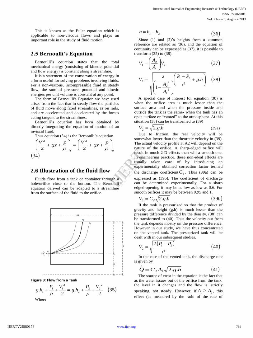
2.6 Illustration of the fluid flow

Fluids flow from a tank or container through a

hole/orifice close to the bottom. The Bernoulli

equation derived can be adapted to a streamline

from the surface of the fluid to the orifice.

Figure 3: Flow from a Tank

2.

2.

2

222

2

111

VPhg

VPhg

35

Where

21 hhh 36

Since (1) and (2)’s heights from a common

reference are related as (36), and the equation of

continuity can be expressed as (37), it is possible to

transform (35) to (38).

2

1

21 .V

A

AV

37

hgPP

A

AV .

1

2 21

2

1

2

2

2

38

A special case of interest for equation (38) is

when the orifice area is much lesser than the

surface area and when the pressure inside and

outside the tank is the same- when the tank has an

open surface or “vented” to the atmosphere. At this

situation (38) can be transformed to (39)

hgV ..22 (39a)

Due to friction, the real velocity will be

somewhat lower than the theoretic velocity in (39).

The actual velocity profile at A2 will depend on the

nature of the orifice. A sharp-edged orifice will

result in much 2-D effects than will a smooth one.

In engineering practice, these non-ideal effects are

usually taken care of by introducing an

experimentally obtained correction factor termed

the discharge coefficient dC . Thus (39a) can be

expressed as (39b). The coefficient of discharge

can be determined experimentally. For a sharp

edged opening it may be as low as low as 0.6. For

smooth orifices it may be between 0.95 and 1.

hgCV d ..22 b39

If the tank is pressurized so that the product of

gravity and height (g.h) is much lesser than the

pressure difference divided by the density, (38) can

be transformed to (40). Thus the velocity out from

the tank depends mostly on the pressure difference.

However in our study, we have thus concentrated

on the vented tank. The pressurized tank will be

dealt with in our subsequent studies.

212

.2 PPV

40

In the case of the vented tank, the discharge rate

is given by

hgACQ d ..22

41

The source of error in the equation is the fact that

as the water issues out of the orifice from the tank,

the level in it changes and the flow is, strictly

speaking, not steady. However, if 21 AA , this

effect (as measured by the ratio of the rate of

786



IJERT

IJERT

ISSN: 2278-0181


change in the level and velocity 2V ), is so small

that the error made is insignificant.

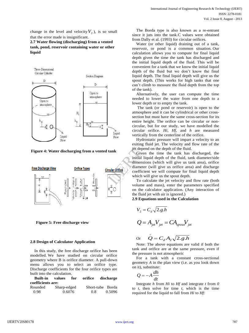
2.7 Water flowing (discharging) from a vented

tank, pond, reservoir containing water or other

liquid

Figure 4: Water discharging from a vented tank

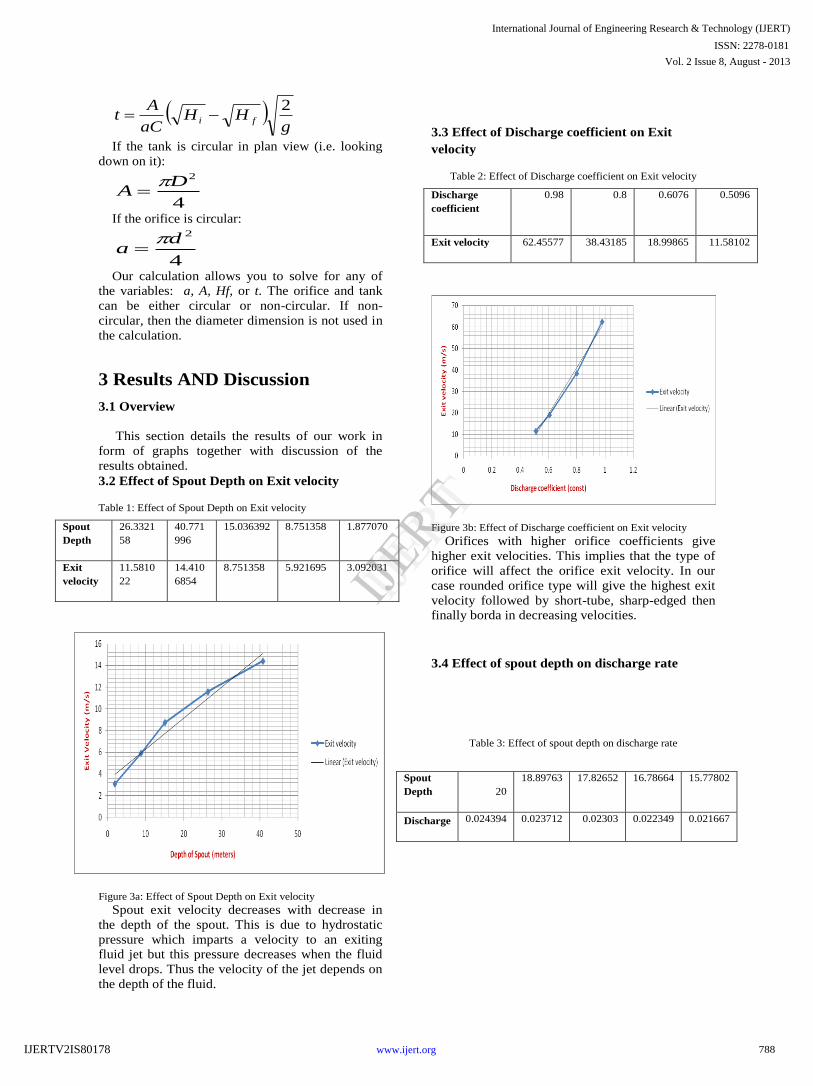
Figure 5: Free discharge view

2.8 Design of Calculator Application

In this study, the free discharge orifice has been

modelled. We have studied on circular orifice

geometry where B is orifice diameter. A pull-down

menu allows you to select an orifice type.

Discharge coefficients for the four orifice types are

built into the calculation.

Built-in values for orifice discharge

coefficients are: Rounded Sharp-edged Short-tube Borda

0.98 0.6076 0.8 0.5096

The Borda type is also known as a re-entrant

since it juts into the tank.C values were obtained

from Dally et al. (1993) for circular orifices.

Water (or other liquid) draining out of a tank,

reservoir, or pond is a common situation. Our

calculation allows you to compute for final liquid

depth given the time the tank has discharged and

the initial liquid depth of the fluid. This will be

convenient for a tank that we know the initial liquid

depth of the fluid but we don’t know the final

liquid depth. The final liquid depth will give us the

spout depth. (This works for high tanks that one

can’t climb to measure the fluid depth from the top

of the tank).

Alternatively, the user can compute the time

needed to lower the water from one depth to a

lower depth or to empty the tank.

The tank (or pond or reservoir) is open to the

atmosphere and it can be cylindrical or other cross-

section but must have the same cross-section for its

entire height. The orifice can be circular or non-

circular, but for our study, we have modelled the

circular orifice. Hi, Hf, and h are measured

vertically from the centerline of the orifice.

Hydrostatic pressure will impart a velocity to an

exiting fluid jet. The velocity and flow rate of the

jet depend on the depth of the fluid.

Given the time the tank has discharged, the

initial liquid depth of the fluid, tank diameter/side

dimensions (which will give us tank area), orifice

diameter (will give us orifice area) and discharge

coefficient we will compute for final liquid depth

which will give us the spout depth.

To calculate the jet velocity and flow rate (both

volume and mass), enter the parameters specified

on the calculator application. (Any interaction of

the fluid jet with air is ignored.)

2.9 Equations used in the Calculation

hgCV d ..22

jetspoutjetjet VCAVAQ

Or hgACQ d ..22

Note: The above equations are valid if both the

tank and orifice are at the same pressure, even if

the pressure is not atmospheric

For a tank with a constant cross-sectional

geometry A in the plan view (i.e. as you look down

on it), substitute:

dt

dhAQ

Integrate h from Hi to Hf and integrate t from 0

to t, then solve for time t, which is the time

required for the liquid to fall from Hi to Hf:

787



IJERT

IJERT

ISSN: 2278-0181


g

HHaC

At fi

2

If the tank is circular in plan view (i.e. looking

down on it):

4

2DA

If the orifice is circular:

4

2da

Our calculation allows you to solve for any of

the variables: a, A, Hf, or t. The orifice and tank

can be either circular or non-circular. If non-

circular, then the diameter dimension is not used in

the calculation.

3 Results AND Discussion

3.1 Overview

This section details the results of our work in

form of graphs together with discussion of the

results obtained.

3.2 Effect of Spout Depth on Exit velocity

Table 1: Effect of Spout Depth on Exit velocity

Spout

Depth

26.3321

58

40.771

996

15.036392 8.751358 1.877070

Exit

velocity

11.5810

22

14.410

6854

8.751358 5.921695 3.092031

Figure 3a: Effect of Spout Depth on Exit velocity

Spout exit velocity decreases with decrease in

the depth of the spout. This is due to hydrostatic

pressure which imparts a velocity to an exiting

fluid jet but this pressure decreases when the fluid

level drops. Thus the velocity of the jet depends on

the depth of the fluid.

3.3 Effect of Discharge coefficient on Exit

velocity

Table 2: Effect of Discharge coefficient on Exit velocity

Discharge

coefficient

0.98 0.8 0.6076 0.5096

Exit velocity 62.45577 38.43185 18.99865 11.58102

Figure 3b: Effect of Discharge coefficient on Exit velocity

Orifices with higher orifice coefficients give

higher exit velocities. This implies that the type of

orifice will affect the orifice exit velocity. In our

case rounded orifice type will give the highest exit

velocity followed by short-tube, sharp-edged then

finally borda in decreasing velocities.

3.4 Effect of spout depth on discharge rate

Table 3: Effect of spout depth on discharge rate

Spout

Depth 20

18.89763 17.82652 16.78664 15.77802

Discharge 0.024394 0.023712 0.02303 0.022349 0.021667

788



IJERT

IJERT

ISSN: 2278-0181


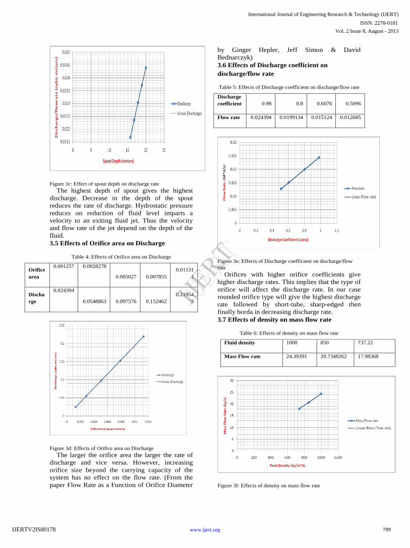
Figure 3c: Effect of spout depth on discharge rate

The highest depth of spout gives the highest

discharge. Decrease in the depth of the spout

reduces the rate of discharge. Hydrostatic pressure

reduces on reduction of fluid level imparts a

velocity to an exiting fluid jet. Thus the velocity

and flow rate of the jet depend on the depth of the

fluid.

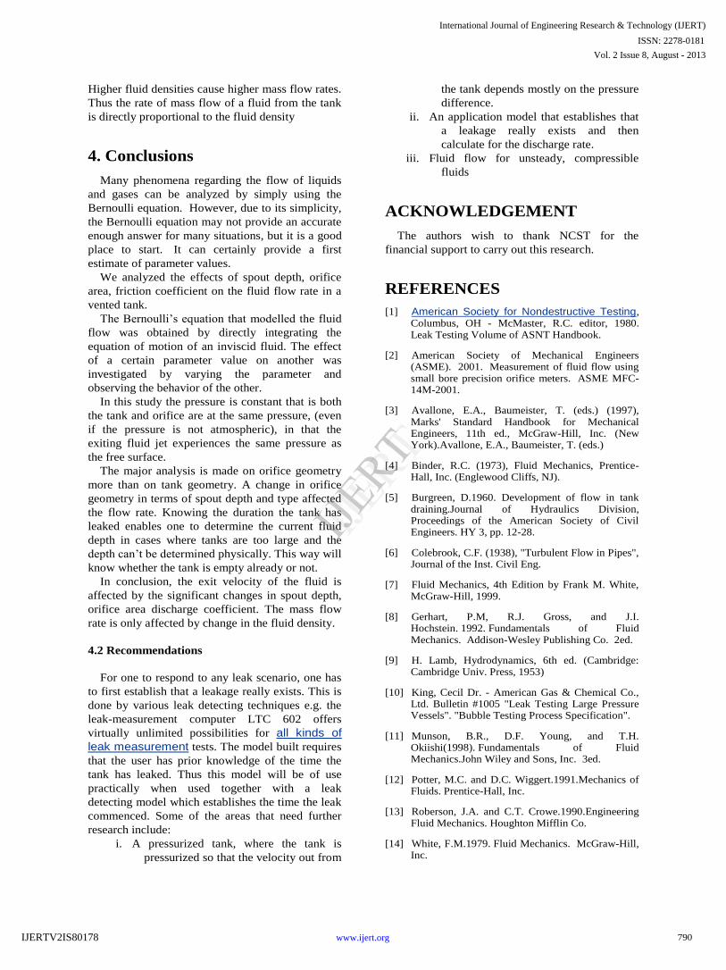
3.5 Effects of Orifice area on Discharge

Table 4: Effects of Orifice area on Discharge

Orifice

area

0.001257 0.0028278

0.005027 0.007855

0.01131

1

Discha

rge

0.024394

0.0548863 0.097576 0.152462

0.21954

5

Figure 3d: Effects of Orifice area on Discharge

The larger the orifice area the larger the rate of

discharge and vice versa. However, increasing

orifice size beyond the carrying capacity of the

system has no effect on the flow rate. (From the

paper Flow Rate as a Function of Orifice Diameter

by Ginger Hepler, Jeff Simon & David

Bednarczyk)

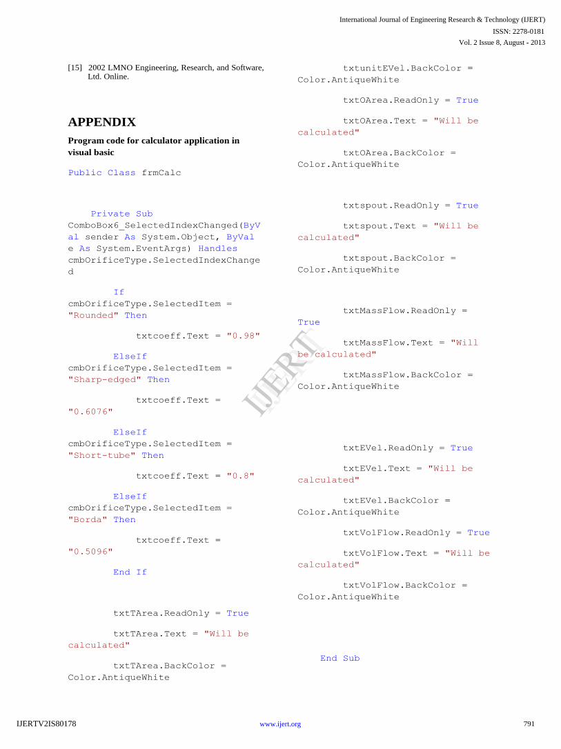
3.6 Effects of Discharge coefficient on

discharge/flow rate

Table 5: Effects of Discharge coefficient on discharge/flow rate

Discharge

coefficient 0.98 0.8 0.6076 0.5096

Flow rate 0.024394 0.0199134 0.015124 0.012685

Figure 3e: Effects of Discharge coefficient on discharge/flow

rate

Orifices with higher orifice coefficients give

higher discharge rates. This implies that the type of

orifice will affect the discharge rate. In our case

rounded orifice type will give the highest discharge

rate followed by short-tube, sharp-edged then

finally borda in decreasing discharge rate.

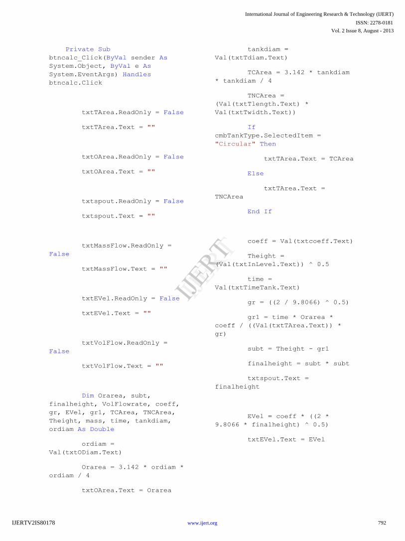
3.7 Effects of density on mass flow rate

Table 6: Effects of density on mass flow rate

Fluid density 1000 850 737.22

Mass Flow rate 24.39391 20.7348262 17.98368

Figure 3f: Effects of density on mass flow rate

789



IJERT

IJERT

ISSN: 2278-0181


Higher fluid densities cause higher mass flow rates.

Thus the rate of mass flow of a fluid from the tank

is directly proportional to the fluid density

4. Conclusions

Many phenomena regarding the flow of liquids

and gases can be analyzed by simply using the

Bernoulli equation. However, due to its simplicity,

the Bernoulli equation may not provide an accurate

enough answer for many situations, but it is a good

place to start. It can certainly provide a first

estimate of parameter values.

We analyzed the effects of spout depth, orifice

area, friction coefficient on the fluid flow rate in a

vented tank.

The Bernoulli’s equation that modelled the fluid

flow was obtained by directly integrating the

equation of motion of an inviscid fluid. The effect

of a certain parameter value on another was

investigated by varying the parameter and

observing the behavior of the other.

In this study the pressure is constant that is both

the tank and orifice are at the same pressure, (even

if the pressure is not atmospheric), in that the

exiting fluid jet experiences the same pressure as

the free surface.

The major analysis is made on orifice geometry

more than on tank geometry. A change in orifice

geometry in terms of spout depth and type affected

the flow rate. Knowing the duration the tank has

leaked enables one to determine the current fluid

depth in cases where tanks are too large and the

depth can’t be determined physically. This way will

know whether the tank is empty already or not.

In conclusion, the exit velocity of the fluid is

affected by the significant changes in spout depth,

orifice area discharge coefficient. The mass flow

rate is only affected by change in the fluid density.

4.2 Recommendations

For one to respond to any leak scenario, one has

to first establish that a leakage really exists. This is

done by various leak detecting techniques e.g. the

leak-measurement computer LTC 602 offers

virtually unlimited possibilities for all kinds of

leak measurement tests. The model built requires

that the user has prior knowledge of the time the

tank has leaked. Thus this model will be of use

practically when used together with a leak

detecting model which establishes the time the leak

commenced. Some of the areas that need further

research include:

i. A pressurized tank, where the tank is

pressurized so that the velocity out from

the tank depends mostly on the pressure

difference.

ii. An application model that establishes that

a leakage really exists and then

calculate for the discharge rate.

iii. Fluid flow for unsteady, compressible

fluids

ACKNOWLEDGEMENT

The authors wish to thank NCST for the

financial support to carry out this research.

REFERENCES

[1] American Society for Nondestructive Testing, Columbus, OH - McMaster, R.C. editor, 1980. Leak Testing Volume of ASNT Handbook.

[2] American Society of Mechanical Engineers (ASME). 2001. Measurement of fluid flow using small bore precision orifice meters. ASME MFC-14M-2001.

[3] Avallone, E.A., Baumeister, T. (eds.) (1997), Marks' Standard Handbook for Mechanical Engineers, 11th ed., McGraw-Hill, Inc. (New York).Avallone, E.A., Baumeister, T. (eds.)

[4] Binder, R.C. (1973), Fluid Mechanics, Prentice-Hall, Inc. (Englewood Cliffs, NJ).

[5] Burgreen, D.1960. Development of flow in tank draining.Journal of Hydraulics Division, Proceedings of the American Society of Civil Engineers. HY 3, pp. 12-28.

[6] Colebrook, C.F. (1938), "Turbulent Flow in Pipes", Journal of the Inst. Civil Eng.

[7] Fluid Mechanics, 4th Edition by Frank M. White, McGraw-Hill, 1999.

[8] Gerhart, P.M, R.J. Gross, and J.I. Hochstein. 1992. Fundamentals of Fluid Mechanics. Addison-Wesley Publishing Co. 2ed.

[9] H. Lamb, Hydrodynamics, 6th ed. (Cambridge: Cambridge Univ. Press, 1953)

[10] King, Cecil Dr. - American Gas & Chemical Co., Ltd. Bulletin #1005 "Leak Testing Large Pressure Vessels". "Bubble Testing Process Specification".

[11] Munson, B.R., D.F. Young, and T.H. Okiishi(1998). Fundamentals of Fluid Mechanics.John Wiley and Sons, Inc. 3ed.

[12] Potter, M.C. and D.C. Wiggert.1991.Mechanics of Fluids. Prentice-Hall, Inc.

[13] Roberson, J.A. and C.T. Crowe.1990.Engineering Fluid Mechanics. Houghton Mifflin Co.

[14] White, F.M.1979. Fluid Mechanics. McGraw-Hill, Inc.

790



IJERT

IJERT

ISSN: 2278-0181


[15] 2002 LMNO Engineering, Research, and Software, Ltd. Online.

APPENDIX

Program code for calculator application in

visual basic

Public Class frmCalc

Private Sub

ComboBox6_SelectedIndexChanged(ByV

al sender As System.Object, ByVal

e As System.EventArgs) Handles

cmbOrificeType.SelectedIndexChange

d

If

cmbOrificeType.SelectedItem =

"Rounded" Then

txtcoeff.Text = "0.98"

ElseIf


"Sharp-edged" Then

txtcoeff.Text =

"0.6076"

ElseIf


"Short-tube" Then

txtcoeff.Text = "0.8"

ElseIf


"Borda" Then

txtcoeff.Text =

"0.5096"

End If

txtTArea.ReadOnly = True

txtTArea.Text = "Will be

calculated"

txtTArea.BackColor =

Color.AntiqueWhite

txtunitEVel.BackColor =

Color.AntiqueWhite

txtOArea.ReadOnly = True

txtOArea.Text = "Will be

calculated"

txtOArea.BackColor =

Color.AntiqueWhite

txtspout.ReadOnly = True

txtspout.Text = "Will be

calculated"

txtspout.BackColor =

Color.AntiqueWhite

txtMassFlow.ReadOnly =

True

txtMassFlow.Text = "Will

be calculated"

txtMassFlow.BackColor =

Color.AntiqueWhite

txtEVel.ReadOnly = True

txtEVel.Text = "Will be

calculated"

txtEVel.BackColor =

Color.AntiqueWhite

txtVolFlow.ReadOnly = True

txtVolFlow.Text = "Will be

calculated"

txtVolFlow.BackColor =

Color.AntiqueWhite

End Sub

791



IJERT

IJERT

ISSN: 2278-0181


Private Sub

btncalc_Click(ByVal sender As

System.Object, ByVal e As

System.EventArgs) Handles

btncalc.Click

txtTArea.ReadOnly = False

txtTArea.Text = ""

txtOArea.ReadOnly = False

txtOArea.Text = ""

txtspout.ReadOnly = False

txtspout.Text = ""

txtMassFlow.ReadOnly =

False

txtMassFlow.Text = ""

txtEVel.ReadOnly = False

txtEVel.Text = ""

txtVolFlow.ReadOnly =

False

txtVolFlow.Text = ""

Dim Orarea, subt,

finalheight, VolFlowrate, coeff,

gr, EVel, gr1, TCArea, TNCArea,

Theight, mass, time, tankdiam,

ordiam As Double

ordiam =

Val(txtODiam.Text)

Orarea = 3.142 * ordiam *

ordiam / 4

txtOArea.Text = Orarea

tankdiam =

Val(txtTdiam.Text)

TCArea = 3.142 * tankdiam

* tankdiam / 4

TNCArea =

(Val(txtTlength.Text) *

Val(txtTwidth.Text))

If

cmbTankType.SelectedItem =

"Circular" Then

txtTArea.Text = TCArea

Else

txtTArea.Text =

TNCArea

End If

coeff = Val(txtcoeff.Text)

Theight =

(Val(txtInLevel.Text)) ^ 0.5

time =

Val(txtTimeTank.Text)

gr = ((2 / 9.8066) ^ 0.5)

gr1 = time * Orarea *

coeff / ((Val(txtTArea.Text)) *

gr)

subt = Theight - gr1

finalheight = subt * subt

txtspout.Text =

finalheight

EVel = coeff * ((2 *

9.8066 * finalheight) ^ 0.5)

txtEVel.Text = EVel

792



IJERT

IJERT

ISSN: 2278-0181


VolFlowrate = Orarea *

coeff * ((2 * 9.8066 *

finalheight) ^ 0.5)

txtVolFlow.Text =

VolFlowrate

mass = VolFlowrate *

Val(txtfluid.Text)

txtMassFlow.Text = mass

txtunitEVel.Text = "m/s"

txtunitMass.Text = "Kg/s"

txtunitOArea.Text =

"Square Metres"

txtunitSpout.Text =

"Metres"

txtunitTArea.Text =

"square Metres"

txtunitVolRate.Text =

"M^3/s"

End Sub

Private Sub

ComboBox1_SelectedIndexChanged(ByV

al sender As System.Object, ByVal

e As System.EventArgs) Handles

cmbTankType.SelectedIndexChanged

If


"Circular" Then

txtTlength.ReadOnly =

True

txtTwidth.ReadOnly =

True

txtTwidth.Text = "Not

Used"

txtTlength.Text = "Not

Used"

txtTdiam.ReadOnly =

False

txtTdiam.Text = ""

Else

txtTdiam.Text = "Not

Used"

txtTwidth.Text = ""

txtTlength.Text = ""

txtTlength.ReadOnly =

False

txtTwidth.ReadOnly =

False

txtTdiam.ReadOnly =

True

End If

End Sub

Private Sub

btnrefresh_Click(ByVal sender As

System.Object, ByVal e As

System.EventArgs) Handles

btnrefresh.Click

txtcoeff.Text = ""

txtEVel.Text = ""

txtfluid.Text = ""

txtInLevel.Text = ""

txtMassFlow.Text = ""

txtOArea.Text = ""

txtODiam.Text = ""

txtspout.Text = ""

txtTArea.Text = ""

txtTdiam.Text = ""

793



IJERT

IJERT

ISSN: 2278-0181


txtTimeTank.Text = ""

txtTlength.Text = ""

txtTwidth.Text = ""

txtunitEVel.Text = ""

txtunitMass.Text = ""

txtunitOArea.Text = ""

txtunitSpout.Text = ""

txtunitTArea.Text = ""

txtunitVolRate.Text = ""

txtVolFlow.Text = ""

cmbOrificeType.SelectedItem = ""


""

End Sub

Private Sub frmCalc_Load(ByVal

sender As System.Object, ByVal e

As System.EventArgs) Handles

MyBase.Load

End Sub

End Class

794



IJERT

IJERT

ISSN: 2278-0181


Some Investigation Of Incompressible Inviscid Steady Flow ... · Some Investigation Of...

Documents

Transcript of Some Investigation Of Incompressible Inviscid Steady Flow ... · Some Investigation Of...