
null hypothesis a,
166
1. Report No. 2. Government Accession No. FHWA/TX-95/1232-28 4. Title and Subtitle A STUDY OF SELECTED WARNING DEVICES FOR REDUCING TRUCK SPEEDS 7. Author(s) Dan Middleton 9. Performing Organization Name and Address Texas Transportation Institute The Texas A&M University System College Station, Texas 77843-3135 12. Sponsoring Agency Name and Address Texas Department of Transportation Research and Technology Transfer Office P. O. Box 5080 Austin, Texas 78763-5080 15. Supplementary Notes Technical Report Documentation Pa2e 3. Recipient's Catalog No. 5. Report Date November 1994 6. Performing Organization Code 8. Performing Organization Report No. Research Report 1232-28 10. Work Unit No. (fRAIS) 11. Contract or Grant No. Study No. 0-1232 13. Type of Report and Period Covered Interim: September 1993 - August 1994 14. Sponsoring Agency Code Research performed in cooperation with the Texas Department of Transportation and the U.S. Department of Transportation, Federal Highway Administration. Research Study Title: Urban Highway Operations Research and Implementation Program 16. Abstract Providing effective roadside warning devices for drivers of large trucks is critical on freeway connectors where speeds are relatively high but design speeds may be substantially lower than on mainlanes. Identifying and testing appropriate methods of monitoring traffic on freeway connectors was included in an earlier phase of this research. Two monitoring systems evolved, one using roadway sensors and the other using roadside sensors. Roadway sensors consisted of both piezoelectric and inductive loop sensors, while roadside sensors applied infrared sensor technology. The roadway warning devices tested can be categorized as passive devices and active devices. Passive devices consisted of "truck tipping" warning signs, while the active device consisted of flashing lights mounted one above and one below a set of passive truck tipping signs on both sides of the roadway. Speed reduction, as associated with accident reduction, was the ultimate goal of these tests. The null hypothesis tested by ANOVA of no treatment effect in the presence of initial speed was rejected in all but one of four models, using the probability of a Type I error, a, equal 0.05. Speed reductions due to the active system were significant downstream of the first curve on the connector, suggesting that truck drivers reduced speeds due to the lights, but beyond the desired location. Cumulative speed distributions showed that the fastest trucks decreased their speeds by approximately 3 to 5 km/h (2 to 3 mi/h) during the test period. Five of the seven single-vehicle truck accidents recorded on the 1-61O/US-59 connector in an 8 112 year period were speed-related, resulting in rollover. None occurred after installation of warning treatments being tested, although there were other prior years before treatment with no recorded accidents. 17. Key Words 18. Distribution Statement Truck Safety, Truck Stability, Truck Speeds, Vehicle Classification, Warning Devices No restrictions. This document is available to the public through NTIS: 19. Security Classif.(ofthis report) Unclassified National Technical Information Service 5285 Port Royal Road Springfield, Virginia 22161 20. Security Classif.(ofthis page) Unclassified 21. No. of Pages 164 22. Price Form DOT F 1700.7 (8-72) Reproduction of completed page authorized
Transcript of null hypothesis a,

1. Report No. 2. Government Accession No.
FHWA/TX-95/1232-28
4. Title and Subtitle
A STUDY OF SELECTED WARNING DEVICES FOR REDUCING TRUCK SPEEDS
7. Author(s)
Dan Middleton
9. Performing Organization Name and Address
Texas Transportation Institute The Texas A&M University System College Station, Texas 77843-3135
12. Sponsoring Agency Name and Address
Texas Department of Transportation Research and Technology Transfer Office P. O. Box 5080 Austin, Texas 78763-5080
15. Supplementary Notes
Technical Report Documentation Pa2e
3. Recipient's Catalog No.
5. Report Date
November 1994
6. Performing Organization Code
8. Performing Organization Report No.
Research Report 1232-28
10. Work Unit No. (fRAIS)
11. Contract or Grant No.
Study No. 0-1232
13. Type of Report and Period Covered
Interim: September 1993 - August 1994
14. Sponsoring Agency Code
Research performed in cooperation with the Texas Department of Transportation and the U.S. Department of Transportation, Federal Highway Administration. Research Study Title: Urban Highway Operations Research and Implementation Program
16. Abstract
Providing effective roadside warning devices for drivers of large trucks is critical on freeway connectors where speeds are relatively high but design speeds may be substantially lower than on mainlanes. Identifying and testing appropriate methods of monitoring traffic on freeway connectors was included in an earlier phase of this research. Two monitoring systems evolved, one using roadway sensors and the other using roadside sensors. Roadway sensors consisted of both piezoelectric and inductive loop sensors, while roadside sensors applied infrared sensor technology. The roadway warning devices tested can be categorized as passive devices and active devices. Passive devices consisted of "truck tipping" warning signs, while the active device consisted of flashing lights mounted one above and one below a set of passive truck tipping signs on both sides of the roadway. Speed reduction, as associated with accident reduction, was the ultimate goal of these tests. The null hypothesis tested by ANOV A of no treatment effect in the presence of initial speed was rejected in all but one of four models, using the probability of a Type I error, a, equal 0.05. Speed reductions due to the active system were significant downstream of the first curve on the connector, suggesting that truck drivers reduced speeds due to the lights, but beyond the desired location. Cumulative speed distributions showed that the fastest trucks decreased their speeds by approximately 3 to 5 km/h (2 to 3 mi/h) during the test period. Five of the seven single-vehicle truck accidents recorded on the 1-61O/US-59 connector in an 8 112 year period were speed-related, resulting in rollover. None occurred after installation of warning treatments being tested, although there were other prior years before treatment with no recorded accidents.
17. Key Words 18. Distribution Statement
Truck Safety, Truck Stability, Truck Speeds, Vehicle Classification, Warning Devices
No restrictions. This document is available to the public through NTIS:
19. Security Classif.(ofthis report)
Unclassified
National Technical Information Service 5285 Port Royal Road Springfield, Virginia 22161
20. Security Classif.(ofthis page)
Unclassified 21. No. of Pages
164 22. Price
~----------~---------, .--~------------------------~------------~----------~ Form DOT F 1700.7 (8-72) Reproduction of completed page authorized


A STUDY OF SELECTED WARNING DEVICES
FOR REDUCING TRUCK SPEEDS
by
Dan Middleton, P .E. Associate Research Engineer Texas Transportation Institute
Research Report 1232-28 Research Study Number 0-1232
Research Study Title: Urban Highway Operations Research and Implementation Program
Sponsored by the Texas Department of Transportation
In Cooperation with U. S. Department of Transportation
Federal Highway Administration
November 1994
TEXAS TRANSPORTATION INSTITUTE The Texas A&M University System College Station, Texas 77843-3135
-- -- -- ---------------------- ------------------------------~-----


IMPLEMENTATION STATEMENT
Findings of this research indicate that excessive speed is a significant factor in singlevehicle large truck crashes. Of the seven single-vehicle truck accidents that were recorded on the 1-610/US-59 connector in an 8 112 year period, excessive speed was noted explicitly by the investigating officer in four. Rollover was a result in five of these seven accidents. Therefore, providing effective vehicle-specific warning devices is deemed important in achieving speed reduction. The literature review, the truck driver interviews, and the speed data collected during this research provided insight into implementation of the warning devices tested.
Driver perceptions and preferences, along with roadway design considerations resulting from this research are pertinent to this discussion. Preferences of truck drivers interviewed in Maryland and Virginia included the following elements: a tipping truck silhouette, a diagrammatic curve arrow, an advisory speed, the legends ROLLOVER HAZARD or TRUCK CAUTION. Legibility testing strongly supported the use of symbolic signs but with a separate advisory speed plate underneath. Finally, truck drivers expressed the desirability of using both advance warning signs and flashing lights in combination with these at-ramp signs.
Statements of Texas truck drivers regarding advisory speeds revealed that they believe speeds are set for automobiles, requiring trucks to travel even slower than posted speeds to be safe. However, these comments from both groups of Texas drivers were inconsistent with findings of actual speeds on the I-61O/US-59 connector and with the author's observations of trucks elsewhere.
Values of side friction accepted by drivers on the first curve of the subject connector were significantly higher than the 0.15 value proposed by the Green Book for a 64 km/ h (40 mi/h) design speed. The 95th percentile speed on the subject connector of 93 km/h (58 mi/h) implied a side friction factor of 0.39 while the 10th percentile car drivers accepted a value of 0.18. It should also be noted that these relatively high values might also reflect driver inability to judge the sharpness of the curve in advance.
On horizontal curves with lower design speeds that are designed in accordance with Green Book Table m-6, the most unstable trucks can roll over when traveling as little as 8 to 16 km/h (5 to 10 mi/h) over the design speed. This is a particular concern on freeway ramps, many of which have unrealistically low design speeds in comparison to mainlanes.
Indicators that should be used to determine the success of warning treatments include not only reductions in accidents but changes in mean speeds and reductions in the speeds of the fastest trucks. This research monitored truck speeds at the beginning of the connector (called Location A), at the beginning of the first curve (Location B), and at the beginning of the second curve (Location C). Speed differences tested for statistical significance included those between A and B, A and C, and Band C. These will be referred to as AB, AC, and BC, respectively. These statistical tests account for initial speeds at either A or B, as signified by either A or B in parentheses. For example, BC(B) refers to the speed difference between B and C using the initial speed at B.
v

Statistical tests used the Analysis of Variance (ANOVA) to test the means of speed reductions and found that treatment was significant (in the presence of initial speed) in the AB, BC(B), and AC(A) data sets. In these tests, samples were large enough that a small difference in sample means was determined to be statistically significant. However, these differences were not practically significant. For example, the most effective treatment in the AB data set was Treatment Condition (TC) 5 whose resulting mean speed reduction was 9.95 km/h (5.83 milh). By comparison, TC 4 resulted in the least speed reduction of 8.74 km/h (5.43 milh) for a difference between the highest and lowest speed reduction of only 0.64 km/h (0.40 milh).
The magnitude of speed reductions of the fastest trucks were greater than reductions in mean speeds among treatment conditions. Speed reductions of the 85th and 95th percentile trucks steadily declined as additional treatments were added, accomplishing consistent reductions at all three monitoring locations of approximately 4.8 kmlh (3 milh). This rmding reinforces the results of the ANOV A, which show TC 5 as the most effective treatment in most cases. Because only the fastest trucks (generally over 88 kmlh (55 milh) at A) would have activated the flashing lights, the incremental effect of the lights on 85th and 95th percentile speeds is obvious. The improvement in speed reduction for TC 5 compared to TC 4 ranges from 0 to 3.2 km/h (0 to 2 milh). The other consideration for TC 5 was the length of time it was being tested, thus providing both a large data sample for comparison purposes and sufficient time of use to overcome the "novelty" effect.
The modest speed reductions indicated by the changes in sample means were disappointing. However, the fastest trucks apparently reduced their speeds as the testing of treatment conditions progressed and as the number of warning devices on the connector increased. This reduction, albeit small in magnitude, might have been sufficient to prevent rollovers of some high center-ofgravity (c.g.) trucks, given that there were no rollovers during the test period, according to accident reports. The sponsor of this research, the Texas Department of Transportation, is considering the use of some or all of these devices on other freeway connectors with implementation in the near future. It is recommended that widespread usage and/or adoption of truck tipping signs into the Texas Manual on Uniform Traffic Control Devices (12) for general use be delayed until supporting evidence of their effectiveness can be demonstrated.
vi

DISCLAIMER
The contents of this report reflect the views of the author who is responsible for the facts and the accuracy of the data presented herein. The contents do not necessarily reflect the official view or policies of the Texas Department of Transportation or of the Federal Highway Administration. This report does not constitute a standard, specification, or regulation. The engineer in charge of the project was Dan Middleton, P.E. # 60764.
vii


TABLE OF CONTENTS
LIST OF FIGURES . . . . . . . . . . . . . . . . . . . . . . . . . . . . . . . . . . . . . . . . . . .. xiii
LIST OF TABLES ............................................ xiv
SUl\IIl.\1ARY ................................................ xv
CHAPTER 1. INTRODUCTION .................................. 1
BACKGROUND ......................................... 1
OBJECTIVES ........................................... 1
SITE INFORMATION, ..................................... 2
TIlE PROBLEM ......................................... 5 Houston Freeway Accidents . . . . . . . . . . . . . . . . . . . . . . . . . . . . . . 6 I-610/US-59 Ramp Accident History ........................ 8
CO~EASURES ..................................... 8
TORT IlABillTY ..... . . . . . . . . . . . . . . . . . . . . . . . . . . . . . . . . . .. 11 Background . . . . . . . . . . . . . . . . . . . . . . . . . . . . . . . . . . . . . . .. 11 Tort Liability Implications Related to Active Traffic Devices .......... 12
CHAPTER 2. STUDY PROCEDURE ............................... 13
BACKGROUND ......................................... 13
TRUCK DRIVER INTERVIEWS . . . . . . . . . . . . . . . . . . . . . . . . . . . . . .. 14
TRAFFIC MONITORING SYSTEMS . . . . . . . . . . . . . . . . . . . . . . . . . . .. 14 Roadway Components ................................. 15 Temporary Roadway Sensors . . . . . . . . . . . . . . . . . . . . . . . . . . . .. 15 Permanent Roadway Sensors ............................. 16 Vehicle Classifiers . . . . . . . . . . . . . . . . . . . . . . . . . . . . . . . . . . .. 16 Roadside Sensors . . . . . . . . . . . . . . . . . . . . . . . . . . . . . . . . . . . .. 17
TRAFFIC CONTROL TREATMENTS . . . . . . . . . . . . . . . . . . . . . . . . . .. 18 Treatment Conditions . . . . . . . . . . . . . . . . . . . . . . . . . . . . . . . . .. 18 Passive Devices ..................................... 19 Active Devices . . . . . . . . . . . . . . . . . . . . . . . . . . . . . . . . . . . . .. 19
ix

DATA RETRIEVAL. . . . . . . . . . . . . . . . . . . . . . . . . . . . . . . . . . . . . .. 22
DATA ANALYSIS . . . . . . . . . . . . . . . . . . . . . . . . . . . . . . . . . . . . . . .. 23
Fonnatting the IRD Files ............................... 23 Removing Irrelevant Vehicle Records . . . . . . . . . . . . . . . . . . . . . . .. 25 Matching Pairs of Vehicles at A and B with A and C . . . . . . . . . . . . .. 25 Tracing Vehicles from Site A to Site B to Site C . . . . . . . . . . . . . . . .. 26 Statistical Analysis . . . . . . . . . . . . . . . . . . . . . . . . . . . . . . . . . . .. 26
CHAPTER3. LITERATURE REVIEW . . . . . . . . . . . . . . . . . . . . . . . . . . . . .. 29
INTRODUCTION ........................................ 29
GENERAL TRUCK CRASH STATISTICAL STUDIES ................ 29 Generic Studies of Truck Crashes .......................... 30 Freeway Connector and Ramp Studies ....................... 31
SIMULATION STUDIES OF TRUCK CRASHES . . . . . . . . . . . . . . . . . . .. 32
TRUCK FAILURE MODES . . . . . . . . . . . . . . . . . . . . . . . . . . . . . . . . .. 34 Concerns Regarding Current AASHTO Design . . . . . . . . . . . . . . . . .. 36 Factors that Affect Rollover Threshold . . . . . . . . . . . . . . . . . . . . . .. 38 Rollover Threshold for Design . . . . . . . . . . . . . . . . . . . . . . . . . . .. 40
CHAPTER 4. DRIVER CONSIDERATIONS . . . . . . . . . . . . . . . . . . . . . . . . .. 41
INTRODUCTION ........................................ 41
HUMAN FACTORS . . . . . . . . . . . . . . . . . . . . . . . . . . . . . . . . . . . . . .. 41 Driver Comfort Levels . . . . . . . . . . . . . . . . . . . . . . . . . . . . . . . .. 41 Human Factors Considerations on Freeway Connectors ............ 42
TRUCK DRIVER INTERVIEWS . . . . . . . . . . . . . . . . . . . . . . . . . . . . . .. 44 Driver Interviews in Maryland and Virginia . . . . . . . . . . . . . . . . . . .. 44 Driver Interviews in Texas . . . . . . . . . . . . . . . . . . . . . . . . . . . . . .. 55
CHAPTER 5. DATA ANALYSIS . . . . . . . . . . . . . . . . . . . . . . . . . . . . . . . . .. 65
INTRODUCTION ........................................ 65 Treatment Conditions . . . . . . . . . . . . . . . . . . . . . . . . . . . . . . . . .. 65 Modification of TC 1 Data . . . . . . . . . . . . . . . . . . . . . . . . . . . . . .. 67
x

STATISTICAL TESTS ON TRUCK SPEED DATA. . . . . . . . . . . . . . . . . .. 68 The Analysis of Variance ............................... 68 The Null Hypothesis .................................. 68
EFFECTIVENESS OF TREATMENTS BASED ON SPEEDS ............ 70 Selection of Test Criteria . . . . . . . . . . . . . . . . . . . . . . . . . . . . . . .. 70 General Statistical Results ... . . . . . . . . . . . . . . . . . . . . . . . . . . .. 70 Specific Statistical Results . . . . . . . . . . . . . . . . . . . . . . . . . . . . . .. 72 Speed Reductions of the Fastest Trucks . . . . . . . . . . . . . . . . . . . . . .. 77
COMMENTARY ON TRUCK SPEEDS .......................... 77 A Mathematically Derived Maximum Speed ................... 79 Advisory Speed versus Safe Speed . . . . . . . . . . . . . . . . . . . . . . . . .. 81
EFFECTIVENESS OF TREATMENTS BASED ON CRASH mSTORY ..... 85 Department of Public Safety Records . . . . . . . . . . . . . . . . . . . . . . .. 85 Houston Police Department Incident Records . . . . . . . . . . . . . . . . . .. 85 Case Studies . . . . . . . . . . . . . . . . . . . . . . . . . . . . . . . . . . . . . . .. 85 Case Study Evidence .................................. 89
CHAPTER 6. SlJl\t11.\tIARY ...................................... 91
INTRODUCTION ........................................ 91
STUDY PROCEDURE ..................................... 91
EFFECTS OF WARNING TREATMENTS ........................ 92
SOME DESIGN IMPLICATIONS OF STUDY FINDINGS .............. 93 Driver Considerations . . . . . . . . . . . . . . . . . . . . . . . . . . . . . . . . .. 93 Vehicle Design Parameters .............................. 93 Highway Design Parameters . . . . . . . . . . . . . . . . . . . . . . . . . . . . .. 94
RECOMMENDATIONS BASED ON STUDY FINDINGS .............. 94
LIMITATIONS OF DATA . . . . . . . . . . . . . . . . . . . . . . . . . . . . . . . . . .. 95
RECOMMENDATIONS FOR FUTURE RESEARCH ................. 96 Active Warning Devices .. . . . . . . . . . . . . . . . . . . . . . . . . . . . . .. 96 Passive Warning Devices . . . . . . . . . . . . . . . . . . . . . . . . . . . . . . .. 96 Reevaluate Advisory Speeds . . . . . . . . . . . . . . . . . . . . . . . . . . . . .. 96 Reevaluate Side Friction Factors . . . . . . . . . . . . . . . . . . . . . . . . . .. 97
xi

REFERENCES. . . . . . . . . . . . . . . . . . . . . . . . . . . . . . . . . . . . . . . . . . . . . .. 99
APPENDIX A: IRD CLASSIFICATION AND SPEED BINS . . . . . . . . . . . . . . .. 103
APPENDIX B: PENNSYLVANIA TRUCK TIPPING SIGN ................ 107
APPENDIX C: TEXAS TRUCK DRIVER INTERVIEW MATERIALS. . . . . . . .. 111
APPENDIX D: SAS OUTPUT .................................... 117
xii

Fignre
1-1 1-2 1-3 2-1 2-2 2-3 2-4 2-5 2-6 2-7 2-8 2-9 3-1 3-2 4-1 4-2 4-3 4-4 4-5 4-6 4-7 4-8 5-1 5-2 5-3 5-4
LIST OF FIGURES
1-61O/US-59 Interchange Layout .............................. . 1-610 Eastbound to US-59 Northbound Connector .................... . 1-61O/US-59 Connector Detail ................................ . 48-inch by 48-inch (I.22m by 1.22m) Truck Tipping Signs ............. . Overhead Truck Tipping Sign as Viewed from the WIM Site . . . . . . . . . . . . . . Close-up of Overhead Sign . . . . . . . . . . . . . . . . . . . . . . . . . . . . . . . . . . . Static Signs with Active Flashing Lights . . . . . . . . . . . . . . . . . . . . . . . . . . . Example of an IRD File Header . . . . . . . . . . . . . . . . . . . . . . . . . . . . . . . . Example of Records Before Formatting .......................... . Example of Records Mer Formatting .................. . . . . . . . . . . Example of Output Files . . . . . . . . . . . . . . . . . . . . . . . . . . . . . . . . . . . . . Example Data Set of Matched Vehicles .......................... . Rollover Threshold Values for Various Example Vehicles . . . . . . . . . . . . . . . . Influence of Axle Load Variations on Rollover Threshold . . . . . . . . . . . . . . . . Rating of Signs from Laboratory Number 2 . . . . . . . . . . . . . . . . . . . . . . . . . Rating of Signs from Laboratory Number 3 . . . . . . . . . . . . . . . . . . . . . . . . . Rating of Sign Elements from Laboratory Number 4 . . . . . . . . . . . . . . . . . . . Rating of Sign Meaning from Laboratory Number 5 .................. . Rating of Sign Effectiveness ................................. . Relative Sign Detection Distances . . . . . . . . . . . . . . . . . . . . . . . . . . . . . . . Truck Tipping Sign Used in First Interview Session .................. . Truck Tipping Signs Used in Second Interview Session ................ . Pictorial of Treatment Conditions . . . . . . . . . . . . . . . . . . . . . . . . . . . . . . . Cumulative Speed Distribution Values for Location A Cumulative Speed Distribution Values for Location B Cumulative Speed Distribution Values for Location C
xiii
2 3 4
20 20 21 21 24 24 24 25 26 39 39 46 48 49 51 52 53 56 57 66 78 78 79
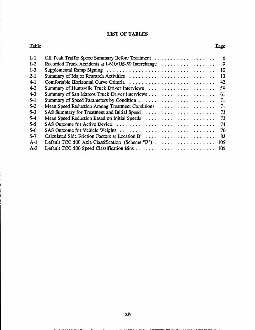
LIST OF TABLES
Table
1-1 Off-Peak Traffic Speed Summary Before Treatment ................... 6 1-2 Recorded Truck Accidents at I-610/US-59 Interchange ................. 9 1-3 Supplemental Ramp Signing .................................. 10 2-1 Summary of Major Research Activities ........................... 13 4-1 Comfortable Horizontal Curve Criteria ........................... 42 4-2 Summary of Huntsville Truck Driver Interviews ..................... 59 4-3 Summary of San Marcos Truck Driver Interviews. . . . . . . . . . . . . . . . . . . .. 61 5-1 Summary of Speed Parameters by Condition . . . . . . . . . . . . . . . . . . . . . . .. 71 5-2 Mean Speed Reduction Among Treatment Conditions .................. 71 5-3 SAS Summary for Treatment and Initial Speed ...... ~ . . . . . . . . . . . . . . .. 73 5-4 Mean Speed Reduction Based on Initial Speeds ...................... 73 5-5 SAS Outcome for Active Device ............................... 74 5-6 SAS Outcome for Vehicle Weights . . . . . . . . . . . . . . . . . . . . . . . . . . . . .. 76 5-7 Calculated Side Friction Factors at Location B I •••••••••••••••••••••• 83 A-I Default TCC 500 Axle Classification (Scheme "F") ................... 105 A-2 Default TCC 500 Speed Classification Bins ......................... 105
xiv

SUMMARY
Providing effective roadside warning devices for drivers of large trucks is critical on freeway connectors where speeds are relatively high but design speeds may be substantially less than on mainlanes. Identifying and testing appropriate methods of monitoring traffic on freeway connectors was also included in this research. Two monitoring systems evolved, one using roadway sensors and the other using roadside sensors. Roadway sensors consisted of both piezoelectric and inductive loop sensors, while roadside sensors applied infrared sensor technology.
The roadway warning devices tested can be categorized as passive devices and active devices. Passive devices consisted of "truck tipping" warning signs, while the active device consisted of flashing lights mounted one above and one below a set of passive truck tipping signs on both sides of the roadway.
Speed reduction, as associated with accident reduction, was the ultimate goal of these tests. The null hypothesis tested by Analysis of Variance (ANOVA) of no treatment effect in the presence of initial speed was rejected in all but one of four models, using the probability of a Type I error and a equal to 0.05. Based on ANOVA results, speed reductions due to the active system substantially occurred downstream of the point of curvature of the first curve, indicating that drivers either did not have sufficient reaction time after the lights came on or they chose to maintain a relatively high speed as long as possible and did not decelerate until they could visually verify the hazard. Truck weights were not significant in any tenable test results, and separation of trucks into the categories of combination and non-combination trucks, peak! off-peak periods, and day/night/dusk periods was not helpful in understanding variations in truck speeds. Cumulative speed distributions showed that the fastest trucks decreased their speeds by approximately 3 to 5 km/h (2 to 3 mi/h) during the test period.
Five of the seven single-vehicle truck accidents recorded on the 1-610/US-59 connector in an 8 112 year period were speed-related and resulted in rollover. None occurred after installation of warning treatments being tested, although there were other prior years with no recorded accidents.
xv


CHAPTER 1. INTRODUCTION
BACKGROUND
Historically, geometric design of roadways has been based on the concept of applying known features of a "design vehicle II to control critical elements of the roadway. Driver characteristics must also be considered, but human performance characteristics are relatively stable over time, requiring less emphasis. Therefore, roadway design requires appropriately selecting the design vehicle of known measurable performance characteristics, predicting the consumer and political dynamics affecting the design vehicle, and predicting the number of these vehicles over some design period. Several roadway design elements currently being used in the 1990 version of A Policy on Geometric Design of Highways and Streets (1) (the Green Book) by the American Association of State Highway and Transportation Officials' (AASHTO) use the passenger car implicitly and explicitly as the design vehicle. Even though the awareness of trucks and their consideration in design has increased over the past 30 years, many existing design features remain as reminders of design practice promulgated by predecessors of the current Green Book (2, J, 1). During this time period, truck sizes and weights have increased significantly, as have their numbers.
OBJECTIVES
The purpose of this research was to investigate the effectiveness of traffic control devices for reducing the speeds of large trucks where potentially hazardous conditions exist on freeway to freeway connectors. Objectives used to accomplish this goal are included in the following:
1. To design and build (or purchase off-the-shelf) systems to monitor and store truck classification and speed data,
2. To identify appropriate static warning devices specifically for truck drivers, 3. To design and build (or purchase) an active warning system that would be activated
by trucks, 4. To install and evaluate the effects of static warning devices for warning truck drivers, 5. To install and evaluate the effects of active warning devices for warning truck drivers,
and 6. To evaluate truck speed data to determine effects of the treatments.
SITE INFORMATION
This ramp is located north of downtown Houston at the interchange of I -61 0 (North Loop) and US-59 (Eastex Freeway). The I-610 eastbound connector to US-59 northbound is the facility that is under investigation. Figure 1-1 shows the general alignment of the ramp and its relationship to other elements of the interchange. Figures 1-2 and 1-3 show additional details regarding data collection equipment and traffic control devices tested in this research. The connector has two lanes which narrow to one lane at its downstream end before the merge with US-59. Because of its height above natural ground level, high speeds, truck volumes, and two 12-degree horizontal curves, it has become a particularly troublesome location.
1

US 59 EASTEX FlfY
Figure 1-1. I-610/US-59 Interchange Layout
2

III
'"
, " '" III ,,' , " '"
Truck Tipping Signs
Localion© . C '<l
Sensors
Lane Ends Merge
Figure 1-2. 1-610 Eastbound to US-59 Northbound Connector

LEGEND
-t CTR System
CJ Inductive Loop (6X8)
181 Cabinet
I Piezoelectric Sensor
Figure 1-3. 1-610IUS-59 Connector Detail
Truck Tipping Signs W/Flashers

Both of the horizontal curves on the connector use compound curve designs to approximate a spiral or transition leading into the 12-degree curves. The degree of curvature, liD, II progresses from a tangent section to 2 degrees, then to 7 degrees, and finally to 12 degrees, and then in reverse order to 7 degrees, to 2 degrees, and then to a tangent section again. The maximum superelevation ("e") is 0.08 mlm (0.08 ftlft), the lane widths are 3.7 m (12 ft), and the left and right shoulder widths are 1.8 m (6 ft) and 3.0 m (10 ft), respectively.
Traffic control devices on this connector prior to placing the truck warning devices consisted of a black on yellow RAMP 40 MPH sign near the gore, a set of black on yellow curve warning signs (one on each side) upstream of each curve, and one LANE ENDS MERGE LEFT warning sign mounted on the right hand side near the second curve. The advisory speed used with the first curve warning sign was 40 kmlh (25 milh) and for the second sign, it was 56 kmlh (35 milh).
Speeds of trucks on the ramp generally decrease from the beginning (gore area) of the ramp to the second curve, then increase gradually along the downgrade from the second curve to the merge area on the Eastex Freeway. Speed reductions by smaller vehicles are not as pronounced as for trucks. Off-peak speeds for various classes of vehicles recorded by the International Road Dynamics (IRD) classifiers are shown by Table 1-1. The vehicle functional classes are consistent with the Federal Highway Administration (FHW A) classification scheme. Classes 1 and 2 are motorcycles and automobiles, classes 3 through 5 are light- to medium-duty trucks, vans, and buses, and classes 6 through 13 are heavy trucks. Due to a problem with the Location A classifier on June 16, 1992, the next closest date (June 25, 1992) was selected to represent speeds at A for comparison purposes.
The average daily traffic volume as counted by the IRD classifiers for a seven-day period at Location A beginning June 17, 1992 was 11,924 vehicles per day (vpd). For the Wednesday of this week (typical of weekdays), the total traffic volume counted was 12,251 vehicles (10.2 percent trucks functional class 4 through 13). Appendix A includes a list of vehicles by functional class as defined by the Federal Highway Administration's Traffic Monitoring Guide (~). Sixty-nine percent of the class 4 through 13 trucks were in the right lane at Location A, according to the IRD classification count. The IRD count for the Saturday of this week was 11,408 vehicles (6.2 percent trucks of functional class 4 through 13).
THE PROBLEM
The unique characteristics of large trucks require special attention by design and operations engineers in order to maintain the safest possible environment for all vehicles, especially where constraining geometric elements exist. Freeway to freeway connectors are examples of roadways where speed reductions are necessary due to combinations of horizontal curves, vertical curves, and grades. Motorists exiting a high-speed freeway, utilizing a freeway to freeway connector, tend to maintain a certain momentum due, at least in part, to the merge downstream with high-speed traffic on another freeway. Combining this tendency to maintain high speeds with the relatively poor stability performance aspects of large trucks represents an increase in the hazard potential.
The involvement of large trucks can exacerbate the damage and delay aspects of freeway crashes and/or incidents. The truck's large size and the potential for spilled cargo, combined in some cases with special handling requirements of hazardous materials, requires that special care
5

Table 1-1. Off-Peak Traffic Speed Summary Before Treatment
Location Functional (Date) Class n Maximum Minimum Mean Std. Dev.
Loc. A 1-2 1197 196 40 90.5 9.7
(6/25192) 3-5 31 179 32 72.9 19.3
6-13 105 105 32 81.6 15.3
Loc.B 1-2 2662 124 39 84.7 8.5
(6/16/92) 3.5 62 98 32 69.6 16.7
6-13 277 105 40 78.2 10.3
Loc. C 1-2 2340 135 34 77.8 8.1
(6/16/92) 3-5 40 90 35 66.8 11.8
l'i-B 2:)1 R7 ~4 l'iR_7 R_7
Note: Speeds are in units of km/h.
be exercised in providing adequate warning specifically for truck drivers when existing roadway geometric features are unusually demanding.
Houston Freeway Accidents
Based on the activity log of the Accident Division of the City of Houston Police Department (HPD) over a three-month period, approximately one-third of the incidents to which police responded on freeway-to-freeway connectors were attributable to excessive speeds. When large trucks are involved, incidents can be catastrophic, especially when the incident occurs at an interchange where spilled loads alone can disrupt traffic for several hours. Examples of incidents which have resulted in loss of life and extensive damage to the roadway infrastructure are:
1) An ammonia truck incident in May 1976 at 1-610 (West Loop) and US 59 (Southwest Freeway) interchange,
2) A propane and gravel truck collision at the SH 225 (La Porte Freeway) and 1-610 interchange where a police officer died and a connector was closed for a year and a half, and
3) A truck incident on July 30, 1985 in which the driver died and disrupted traffic at the 1-610 and SH 225 (La Porte Freeway) interchange for several hours.
6

Several treatments have been considered at various freeway-to-freeway connectors in Houston based on: accident/incident history, truck volume, incidents attributable to excessive speeds, and consensus of members of the HPD Accident Division. At the 1-610 (North Loop) eastbound to US 59 (Eastex Freeway) northbound connector, the HPD tried speed enforcement by use of radar following installation of regulatory speed limits. Resulting speeds did not indicate the desired speed reduction. Other options, which are the subject of ongoing study, required the installation of sensors of various types and configurations to monitor the effects of varied traffic warning devices. Assessment of traffic monitoring devices and testing warning systems to reduce truck speeds are the subject of this research.
A current study (6) being conducted by Texas Transportation Institute (TTl) utilized two databases of Houston agencies in an evaluation of major incidents on Houston freeways. The HPD Motorcycle Patrol Division provided incident data for major freeway incidents and the Houston Fire Department (HFD) provided their hazardous material database, which included all responses made by the HFD response team during 1991 and 1992. Of the total 157 incidents reported as occurring on freeways, 98 were coded as collision or overturning accidents of vehicles carrying hazardous materials. The mean clearance time for these vehicles was 51 minutes, with a range from near zero to over 6.5 hours.
The HPD motorcycle division documented major incidents, defmed as those that blocked one or more freeway lanes for a duration of longer than 30 minutes. The database used for the TTl study spanned a time period from 1986 through 1992, yielding 612 incidents that occurred on all of the 10 major freeway segments within the HPD jurisdiction. The HPD database covers their hours of operation, which are between the hours of 4 a.m. and 10 p.m. daily.
The TIl analysis included a comparison of incident rates near major freeway to freeway interchanges versus rates between interchanges. This was accomplished by using Block Number information included in the database. Incident rates for all vehicles were 3.5 times greater within interchange areas than they were between interchanges. Of the 612 incidents in the database, 498 (81 percent) involved trucks even though truck traffic accounts for only 7.7 percent of total freeway vehicle miles traveled in Houston. System wide, the truck incident rate was 7.19 incidents per 100 million vehicle kilometers (MVK) (11.57 incidents per 100 million vehicle miles [MVM]); or stated another way, truck incidents occur once every 13.8 MVK (8.6 MVM) of truck travel. By contrast, major incidents involving automobiles only occur once every 731 MVK (454 MVM) of automobile travel.
The database also illustrates that when truck incidents are "major" as defmed above, they usually involve a lost load and/or an overturned truck. Of the 498 truck incidents, 198 (40 percent) were overturned trucks, and 233 (46.8 percent) involved a spilled load. These two categories are not mutually exclusive; however, both require special heavy-duty equipment to clear, increasing the incident duration. The median clearance time for overturned truck incidents was slightly more than 3 hours, compared to a 2.2 hour median clearance time for auto incidents and a 2.4 hour time for all truck incidents combined.
7

Comparing the number of truck accidents that occurred in Houston during this same time period indicates that the 498 major incidents are only a small fraction of the accident data set. According to accident records for 1986 through 1992, there were approximately 7,300 freeway accidents recorded in the Houston area involving trucks (10.7 percent of all accidents during that period). The 498 major incidents are only 6.8 percent of the total accidents, suggesting that the majority of truck-involved incidents are not major incidents as defmed above.
1-610/US-59 Ramp Accident History
Table 1-2 contains a summary of truck accidents at the I-61O/US-59 connector for the time period from January 1, 1985 to July 1,1993, according to Texas Department of Public Safety (DPS) accident reports. Unfortunately, some of these accident reports did not provide the desired level of detail, but details were sufficient to determine the approximate location of the accident on the ramp and whether the accident was speed-related. In addition to accidents recorded by DPS, there were incidents on this connector that were recorded by the HPD Motorcycle Division. Their records indicate one spilled load on February 11, 1988 and one truck rollover on June 20, 1989. However, the spilled load incident in 1988 was not conclusively the result of excessive speed. (See Case Study Number 1 in Chapter 5 for more details.) From January 1989 to November 1993, HPD recorded no additional incidents for the subject connector. The DPS and HPD databases were mutually exclusive with the exception of the June 20, 1989 incident.
COUNTERMEASURES
Because reconstruction of problematic freeway to freeway connectors is usually not feasible, other cost-effective countermeasures are used, at least in the short term. Middleton et al. (1), recently reported on truck accident countermeasures used on freeway ramps, including warning signs, oversize barriers, continuously flashing lights, and increased superelevation. Various warning signs are available in the Manual on Uniform Traffic Control Devices (MUTCD) (8). In addition to the standard ramp speed warning signs (W13-2 and W13-3 in the MUTCD) and warning signs used in advance of, or within curves (chevrons, large arrow signs, curve warning signs, and curve tum signs), some states have used "truck tipping" signs. This sign uses black on yellow colors and shows a tipping truck silhouette and an arrow (pictograph), intended to depict the ramp alignment. Most of these are diamond-shaped warning signs; many include the speed value (in mi/h) on this sign face, while others utilize an advisory speed plate underneath.
In a recent study, Knoblauch and Nitzburg (9) contacted 15 states to identify traffic control devices used at interchange ramps with histories of rollover accidents. Many of the states used variations of the standard MUTCD traffic control devices; others increased the size and/or number of devices or attempted innovative approaches at known problem locations. Although many of the innovative solutions were thought to have reduced the problem, none were formally evaluated. Table 1-3 summarizes the truck accident countermeasures used by these 15 states. Knoblauch and Nitzburg (9) conducted their own field tests at two interchange ramps in Virginia and Maryland to analyze reductions in truck speeds with activation of flashing beacons mounted on truck tipping signs. Results showed that neither large combination vehicles in general nor high center-ofgravity trucks in particular were affected by the treatments. These researchers concluded that even
8

Table 1-2. Recorded Truck Accidents at I-610/US-59 Interchange
Accident First Year Number Date Time Weather Harmful
Event
1985 No Recorded Accidents or Incidents
1986 No Recorded Accidents or Incidents
1987 No Recorded Accidents or Incidents
1988 8074142 3/17 6:30pm WindylRain Rollover
8311601 10/22 1:30pm Unknown Struck
1989 9178889 6/20 3:30pm Cloudy/Dry Rollover
1990 0133198 5/9 3:00pm Clear/Dry Rollover
0170396 6/13 1:40 am Clear/Dry Rollover
0230940 7/30 3:00pm Clear/Dry Rollovera
0337963 11122 12:34 pm Clear/Dry Swerved!
0343710 11128 10:30 am Clear/Dry Lost load
0355792 12/9 5:00pm ClearlDry Rollover
1991 No Recorded Accidents or Incidents
1992 No Recorded Accidents or Incidents
1993 No Recorded Accidents or Incidents a At downstream end of ramp in merge area. b Swerved to avoid another vehicle and rolled over. Source: Texas Department of Public Safety
Total Severity Ann.
Ace.
0
0
0
I 2
PDQ
PDQ 1
PDQ 6
PDQ
I
I
I
I
0
0
0
though speed reductions were not noticeable, the high level of truck driver understanding of these signs was sufficient to consider them at high accident locations.
Two other research initiatives installed warning devices to warn truck drivers of potentially hazardous conditions, but only one of them provided results showing effectiveness of treatments. The first is a study sponsored by the Federal Highway Administration, titled Feasibility of an Automatic Truck Warning System (10). The report provides details on the design, costs, and cost effectiveness of the three options evaluated, but no infonnation was provided on their effectiveness in reducing truck speeds. Future monitoring of the three Capital Beltway sites in Maryland and Virginia is intended to include such evaluations. The second study, sponsored by the Insurance Institute for Highway Safety (11), utilized a flashing light and truck tipping sign combination similar to that used by Knoblauch and Nitzburg. This study found that mean speeds at mid-ramp
9

; Table 1-3. Supplemental Ramp Signing
Mate Countermeasure
1 Tipping silhouette, 2.44 m by 2.44 m (8 ft by 8 ft) square (not diamond).
2 1) TRUCKS - CURVE TIGHTENS (black on white) for mainlane applications. 2) TRUCKS WATCH - RAMP TIGHTENS (black on yellow) for interchanges. 3) Tipping sign with flashing "25" sign overhead.
3 1) Tipping silhouette with diagrammatic arrow and advisory speed, 2) TRUCKS - CAUTION RAMP TIGHTENS
4 1) Chevrons, 2) Overhead lighting at interchange, 3) Scored concrete rumble strips, and 4) Flashing arrow panels.
5 1) Chevrons and 2) Additional delineation.
6 1) Chevrons and 2) Tipping silhouette 610 mm by 610 mm (48 inch by 48 inch) mounted as diamond. Truck always tipping to the right regardless of curve direction.
7 1) Larger than normal advisory speed signs, 2) Move advisory signs upstream.
8 1) Additional signing: RAMP EXIT speed signing, chevrons, horizontal arrows, diagrammatic signs, and double turn warning signs; 2) Rumble strips; 3) Amber flashers on advisory speed signs; 4) Constructed 3.05 m (lO-ft) paved shoulders with cross-hatched paint to improved visibility, 4) TRUCKS TOO FAST WHEN FLASHING activated by trucks at high accident location; 5) TOO FAST FOR CURVE WHEN FLASHING, but not specific to trucks.
9 1) Large Chevrons, 2) Large arrows, 3) Ramp speed signs with diagrammatic arrows, 4) Transverse lane striping, and 5) Additional delineators.
10 1) Chevrons and 2) Diagrammatic arrow of ramp with advisory speed (no truck silhouette).
11 1) Tipping silhouette with diagrammatic arrow, 2) TRUCKS CAUTION LOAD MAY SHIFT, 3) Rumble strips.
12 1) Tipping silhouette with diagrammatic arrow and advisory speed.
13 1) Chevrons, 2) Large arrows, 3) Large arrows with speed advisory, 4) Tipping silhouette (no diagrammatic arrow or advisory speed).
14 1) RAMP _ MPH, 2) Tipping silhouette (no diagrammatic arrow or advisory speed), 3) Large arrow sign.
15 1) Large (1.52 m by 1.52 m [5-ft by 5-ft]) 90 degree turn arrow, 2) 20 MPH with flashing yellow lights.
10

locations were lower when flashing lights were used as compared to speeds during a non-flashing period. Furthermore, even though the flashing lights did not significantly increase compliance of trucks with posted advisory speed signs, they did significantly reduce the number of trucks traveling more than 8 km/h (5 mi/h) and 16 km/h (10 mi/h) faster than the calculated maximum safe speed.
This research tested a warning sign not currently included in the Texas Manual on Uniform Traffic Control Devices (12). However, its use could be effective as a warning specifically for truck drivers where restrictive geometry exists. In addition, the research tests the effectiveness of an "active" warning element which is intended to attract a truck driver's attention to the warning sign and communicate a vehicle-specific message. Active, in this case, means that the traffic warning system is dormant until preset conditions pertaining to vehicle height, speed, and length are met. Passenger cars and most light trucks do not meet the height requirement and will not initiate the active system, no matter how long they are or how fast they are traveling. Only trucks large enough to meet the height and length limits that are exceeding the preset threshold speed will trigger the flashing device. If these devices are effective in reducing truck speeds, it is possible that the number of heavy truck accidents and/or incidents on freeway to freeway connectors will be reduced.
TORT LIABILITY
Background
An issue which is quite significant in the deployment of any traffic control device is tort liability. It is important to consider the implications of installing active warning devices and where governmental entities stand with regard to litigation, should an accident occur. First, the definition of "tort" is a civil wrong, as opposed to a moral or criminal wrong. In highway design and maintenance, a citizen or entity sometimes alleges to have been harmed by the actions of another and can sue in civil court to be awarded damages. Of the five types of torts (libel, slander, assault, trespass, and negligence), the one which is typically involved in lawsuits against governments is the tort of negligence. Negligence, in this context, can be defined as harm occurring to someone (e.g. motorist) or to someone's property by failure of another in government to exercise reasonable, or due care.
Sovereign immunity is another concept inherent to tort liability that needs to be introduced, although a comprehensive discussion of this and other elements related to tort liability are beyond the scope of this study. Sovereign immunity (or governmental immunity) is a legal concept used by governmental entities to defend against tort claims. In essence, the public may not bring suit against a governmental unit unless given permission to do so by that governmental unit. Texas and other states have adopted a tort claims act in which sovereign immunity is voluntarily waived, allowing individuals to sue the government based on losses. The Texas Tort Claims Act, initially introduced in 1967, was vetoed by the governor then and again in 1969. Finally, with modifications to satisfy concerns expressed by the governor, the modified act became law on January 1, 1970. In the Texas Tort Claims Act, sovereign immunity was waived for all governmental units in Texas, meaning that persons were "granted permission" to sue the state or any governmental entity to the extent of the waIver. "Governmental units" included cities, counties, state agencies, and many others.
11
Tort Liability Implications Related to Active Traffic Devices
It is anticipated that the tort of negligence related to active warning devices will be viewed by the courts as similar to two traffic control systems currently being used. These are traffic signals, used for control of vehicular traffic at at-grade intersections, and active railroad grade crossing controls. Both provide measures of comparison, although admittedly there are also differences. Tort claims relative to traffic signal-related accidents are usually based on design deficiencies, timing deficiencies, or improper maintenance. Improper maintenance is perhaps the most pertinent to active signals for trucks, assuming that the design is properly tested and proven and the system initiates and functions properly during an appropriate test period. As with traffic signal maintenance problems, governmental entities must respond within a reasonable amount of time. Notice of a malfunctioning device must be provided before it can be held liable. (This notice may be implied in a case where the defect exists for such a long time period that the governmental unit should have discovered it.) Other factors that have contributed to a finding of negligence are where accurate maintenance records were not kept showing responsiveness to defects, where carelessness or unusual practices in construction or maintenance result in conditions that cause injury, and where the governmental unit did not follow the Texas Manual on Uniform Traffic Control Devices (12).
Making traffic signals "failsafe" is anther means of minimizing losses due to lawsuits. In reality, some problems are beyond practical prevention, but measures need to be taken to ensure a failsafe mode in most situations when failure occurs in normal operation. In the case of intersection signals, the controller goes into a flash mode providing a flashing red signal to all directions of traffic, operationally replicating a STOP sign controlled intersection. Railroad grade crossing signals are also intended to go into a failsafe mode upon loss of power or other problems. Another consideration is that, insofar as practical, traffic control devices should be redundant in the warning conveyed to drivers. In the case of railroad grade crossing signals, there should always be a static sign warning motorists of the crossing in addition to the active signal. Therefore, if a failure occurs in the lights, the static sign still warns motorists of the crossing.
An active warning device for trucks must also contain elements of redundancy; it must be failsafe insomuch as practical; and it must provide a warning to truck drivers even if total loss of power occurs. An element of redundancy is provided by the static sign, which is always visible even if the light system fails. A failsafe mode for the light system would initiate a continuous flashing mode if a failure occurs (other than a complete power outage). A solar panel/battery supply could be provided as an auxiliary power supply to complement other failsafe features.
Past decisions regarding traffic control devices demonstrate how the courts might view a defect in an active device for large trucks. In the case of Henry v. Hack, (13) the courts found that the railroad is chargeable with defects in its warning signs at the crossing in a case where it knew about defects in sufficient time to make corrections. It should be noted that the requirements of highways and railroad do not absolve the motorist of reasonable or due care. All railroad crossings are potentially hazardous, and motorists approaching such crossings must exercise care commensurate with the known danger (14). When motorists are aware of sight distance or other problems that make these railroad crossings even more hazardous, motorists must approach the crossing with even greater care (.li).
12

CHAPTER 2. STUDY PROCEDURE
BACKGROUND
The need for effective speed control on the 1-610 eastbound to US-59 northbound connector became clear based on previous unsuccessful attempts and the crash history of the site. A previous speed control technique included implementing a regulatory speed limit and increased enforcement by the Houston Police Department (HPD) through the use of radar. The end result, according to documentation of speed studies, indicated no clear improvement due to these speed control measures. The regulatory speed limit was subsequently removed. During this time period, the Texas Department of Transportation (TxDOT) and Texas Transportation Institute (TTl) verified existing advisory speed values by using a ball-bank indicator. They determined that the appropriate speed should be 40 kmlh (25 milh) on the first curve and 56 kmlh (35 milh) on the second curve.
In 1990, TTl installed a system of traffic monitoring devices to begin another study of truck speeds on this connector, although there were delays in installing the full complement of equipment to monitor and test truck warning devices. In late 1991 through early 1992, at the request of TxDOT engineers, TTl began planning and designing the actual traffic warning and monitoring systems to supplement those already in place. Monitoring of traffic at Location A (see Figure 1-2) continued during this time period. The primary focus of this document targets the activities occurring during the time period beginning in January 1992 and ending in December 1993. Table 2-1 shows the major phases involved in the study and their time frames.
Table 2-1. Summary of Major Research Activities
TREATMENT DATE CONDITION ACTIVITY
8/5/90 1 nstall cabinet, conduit, and four sets of pavement sensors for monitoring truck speeds.
1/1/92 1 Conduct literature search, plan and conduct truck driver 'nterviews, design, purchase, and test hardware.
5/31/92 1 nstalled 12 piezoelectric film sensors at three locations on the connector to begin system testing and data collection.
6/25/92 2 nstalled four ground-mounted static truck warning signs.
7/21/92 3 nstalled advisory speed plates beneath Phase 2 signs.
8/16/92 4 nstalled large overhead sign near ramp entrance.
11/6/92 5 nstalled active warning system.
5/20/93 5 ~nstalled weigh-in-motion system.
A significant portion of the initial phase of this study was devoted to identifying and testing appropriate methods of monitoring traffic on freeway connectors where the requirement for continuous and uninterrupted communications and electrical power along the connector created unique challenges. It became clear in the early design stages that these challenges would require innovative solutions in order to ensure the project's long-term success.
13

During the hardware design phase, a parallel activity focused on identifying traffic control devices to warn truck drivers of hazards on freeway connectors such as this one. Once a list of static and active warning elements had been identified, the study established a methodical, step-bystep approach to accomplish the project objectives (see Chapter 1). Some of the basic qualifications surrounding this selection process included: 1) use elements in the first phases being tested elsewhere with apparent success, 2) add innovative devices during later phases, 3) avoid legally sensitive elements and/or issues, 4) maintain reasonable costs, 5) consider implications to non-truck drivers, and 6) utilize a phased approach to a multi-staged test.
The preliminary phase of the study included a review of the literature. Based on this review and the author's knowledge of current ongoing research, three static sign designs resulted. Truck driver interview results were used to design both the ground mounted signs and the overhead signs. TxDOT fabricated and installed the passive signs on the connector roadway, and a traffic control consultant installed electrical wiring and hardware for the active phase. The remainder of this chapter provides a more detailed account of the procedures used in the various stages of the research, including the data analysis.
TRUCK DRIVER INTERVIEWS
The primary purpose of truck driver interviews was to determine whether truck drivers in Texas understood the intended meaning of the "truck tipping" sign, which had been used in other states but which had apparently not been used in Texas, at least not extensively. A secondary purpose was to evaluate variations of the dominant standard sign being used in other states. The standard sign plus two alternatives were used to determine truck driver sign recognition and preference among the three choices. If driver recognition results were acceptable, then one of these signs would be proposed for use on the 1-61O/US-59 connector in Houston.
During interviews, information requested from drivers included sign meaning, sign preference among selected alternatives, previous exposure to the sign, their intetpretation of advisory speed plates, and opinions on the effectiveness of flashing yellow lights mounted near signs. Results of these interviews favored the use of the standard truck tipping sign currently used in other states. Details of the interview process and the results are provided in Chapter 4.
TRAFFIC MONITORING SYSTEMS
The design and acquisition phases acquired several components of the various subsystems off-the-shelf, designing and building others as necessary to perform specific functions. The resulting system(s) would need to operate in a stand-alone mode without a human operator for extended periods of time under all weather and traffic conditions. The unique functions required of the systems were: (1) to monitor and store vehicle-specific speed and classification data, (2) to "track" target vehicles from Location A to Location B to Location C to determine speed reduction, (3) to generate an "alarm" in the active phase to initiate a visual stimulus for truck drivers when preset thresholds were met, and 4) to monitor truck weights on "tracked" vehicles. These functions led to installation of three separate, non-integrated systems, although some functions were redundant among the systems.
14

Vehicle classifiers stored speed and classification data (function 1 above) utilizing two types of pavement sensors: temporary sensors mounted on the surface of the roadway and pennanent sensors embedded in the pavement. A system of roadside sensors using infrared (lR) technology performed functions (2) and (3), and a weigh-in-motion system developed by TIl performed function (4). These are described in greater detail below.
Roadway Components
August 5, 1990, was the date when initial installation of components of the traffic monitoring systems began for the subject connector. Included in the initial installations were: an aluminum cabinet mounted on a 760 mm (30-in) aluminum pedestal, 366 m (1,200 ft) of 64 mm (2112 in) diameter conduit welded to the right-hand bridge rail, AC power and a telephone line to the cabinet, and various sensors placed on top of or cut into the pavement. The purpose of the conduit was to protect communications and AC power linkages between control units in or near the cabinet and remote devices installed on the ramp. The initial pavement sensors included several piezoelectric and loop configurations generally located near the beginning of the ramp and both upstream and downstream of the first curve of the ramp.
Upon reevaluation in 1992, the monitoring locations of pavement sensors downstream of the cabinet were modified, and sensor locations near the cabinet changed slightly. The time period used for evaluation of the traffic control devices, which is the focus of this document, began on May 31, 1992. The positioning of sensors installed on this date was designed to capture speeds at the entrance of the ramp and as vehicles entered the two horizontal curves (see Figures 1-2 and 1-3). The first location was adjacent to the cabinet near the ramp gore, the second was at the point of curvature (PC) of the first curve, and the third was at the PC of the second curve. Each monitoring station included the sensors mounted on or in the pavement and a vehicle classifier for recording vehicular information.
Temporary Roadway Sensors
On May 31, 1992, TIl installed 12 "TP" series piezoelectric fIlm sensors manufactured by AMP Incorporated of Valley Forge, Pennsylvania (previously Elf Atochem North America) on the ramp. Figure 1-2 shows the three stations, designated as Locations A, B, and C. The TP sensors generated signals for the three IRD Series 500 classifiers for the duration of the study at Locations B and C, but for a shorter period of time at Location A. The reason was a higher failure rate of TP's at Location A compared to the other two sites and the availability of a back-up system of permanent sensors at Location A. Both cable and film sensors use KYNAR mm as a transducer material. In this application, they transform a mechanical force to an electrical response.
Maintaining the position of these TP sensors was difficult due to the "shoving" action of decelerating vehicles. One method involved the application of a primer which was painted directly on the pavement surface, followed by one layer of a scale tape material called Po1yguard across the entire lane width. After a few minutes of curing time (dependent upon ambient temperature), a new piezo sensor was placed directly on top of and in the center of the Polyguard, being careful
15
to maintain its position relative to the other sensor in the same lane. At least one layer (preferably two layers) of Polyguard covered the sensor in an overlapping fashion to maintain its position relative to the other sensor and to protect it from traffic. Each location typically used 152 mm (six-inch) widths of Polyguard, although 102 mm (four-inch) widths were occasionally used.
Permanent Roadway Sensors
TTl installed one permanent set of sensors on the ramp near the cabinet just downstream of the ramp gore. These sensor sets used two 1.83 m by 2.44 m (six-foot by eight-foot) stranded copper wire inductive loops with one permanent piezoelectric sensor between the two loops in each lane. The general layout is shown in Figure 1-2. To install these sensors, TTl used a pavement saw to cut slots in the pavement to the proper dimensions for both the piezoelectric sensors and the inductive loops. Then, to continue installation of the piezo sensors, the installation crew used flexible aluminum tabs to support the sensor over the slot in the correct position. The next step required backfilling the piezo sensor slot with an epoxy grout, ensuring that the sensor remained in the proper position throughout the pouring and curing process. The piezo-film sensors were placed so that the top surface was 3.2 mm (1/8 in) below the surface of the roadway. When the epoxy had cured sufficiently, the crew placed three layers of scale tape (e.g., Polyguard) over the sensor to ensure that wheel loads were transferred to the sensors underneath. Then, the crew used a sealant material to backfill the inductive loop slots once the three turns of stranded copper wire were in place.
Each permanent piezoelectric sensor consisted of a 25 mm (one-inch) square cross-section U-shaped aluminum channel that contained the piezo-fIlm strip surrounded by an elastomer. The sensor was 1.9 m (75 inches) in length and came equipped with 30 m (100 ft) of coaxial cable. TTl positioned one piezo sensor in each lane in the right-hand wheel path at a 90-degree angle to the direction of traffic. The two inductive loops were placed 5 m (18 ft) apart with the piezo sensor positioned between them. The primary purpose of the inductive loops in this scenario was for speed monitoring; the secondary purpose was to detect the presence of a vehicle.
The permanent sensors, which were installed during the summer of 1990, were the only pavement sensors tested at this site which provided continuous, reliable signals throughout the duration of the study. Unfortunately, these permanent sensors were only installed at Location A; the other two locations were on the actual deck of the bridge, precluding cutting the pavement to submerge the sensors. The only maintenance required from August 1990 to October 1993 was adding Polyguard.
Vehicle Classifiers
Of primary importance in determining the effectiveness of warning devices was the capability of tracking vehicles to determine vehicle-specific speed change from the ramp entry point to critical locations along the ramp. The initial design of the system considered communication by either radio frequency (RF) or copper-wire connections from the cabinet at Location A to monitoring stations. TTl installed AC and solar panel/battery power at the cabinet early in the installation process to be distributed elsewhere on the connector as the need arose.
16

One of the monitoring systems installed near the ftrst curve required AC power, as did the flashing lights which were part of the active trafftc warning system. However, the other monitoring system consisted of three vehicle classifters, each containing its own power source, internal clock, and sufftcient memory capacity to store bin data for over a week or raw data for almost a 24-hour period. Communication among the three units was unnecessary because, by coordinating their internal clocks at the beginning of the data collection period, a vehicle could be "tracked" along the ramp. Unfortunately, tracking vehicles required collecting data in the "raw data" mode, and this mode filled the available memory in less than one day.
The three classifters were International Road Dynamics (IRD) Series 500 vehicle classifters, which received signals from pavement sensors and calculated the vehicle I s speed and axle spacing, and assigned each vehicle to an appropriate class according to a user-specifted "bin" or "raw" mode. Only in the raw data mode could vehicle-speciftc information be stored. This included: speed; date; time in hour, minute, and second; number of axles; vehicle class; and wheelbase.
In the bin mode, classifters stored vehicles in two separate groups: speed bins (generally 8 kmlh [5 milh] increments) and count bins (by vehicle classiftcation). See Appendix A for both classiftcation schemes. However, in the bin mode, there was no way to isolate a particular class of vehicle (e.g. trucks) by speed bin because vehicle classes were aggregated. Vehicle class was based on the Federal Highway Administration (FHW A) classiftcation scheme in the Traffic Monitoring Guide (5).
The IRD system was typically used in the raw data mode so that for each of the three locations on the ramp any vehicle (particularly trucks) could be "tracked" by coordinating the time clocks on all three classifters and calculating the expected travel time between stations. Identiftcation of the same vehicle at each of the three sites was relatively straightforward either manually or by a computer program which matched a vehicle "footprint" at Location A with one which was reasonably close to the same physical dimensions at Band C and which passed the other two locations within a reasonable time window. A later section will describe the program in more detail.
Roadside Sensors
The Center for Transportation Research (CTR) of the University of Texas at Austin installed and tested infrared (IR) sensors at two locations on the I-61O/US-59 ramp to monitor trucks. CTR personnel began testing IR monitoring systems for counting and classifying vehicles in 1988 and installed a system in Houston to detect wrong-way movements on High Occupancy Vehicle lanes in 1989. The system was set to monitor vehicles which are over 4.88 m (16 ft) in length and over 2.16 m (7 ft 1 in) in height. These dimensions reflect those of large trucks which are more likely to have high centers of gravity and thus be subject to rollover. A shorter height is undesirable because sensor beams would be broken by four-tire vans with equipment attached to the roof.
17
Each location initially utilized a two-beam infrared sensor array with the IR source on the right-hand side of the ramp and the receiver on the left-hand side. The sensors were placed 0.61 m (2 ft) apart, oriented at a 90-degree angle to the direction of traffic. A metal pedestal, fastened to the barrier rail by clamps, supported the array. Source and receiver were located approximately 11.59 m (38 ft) apart. The initial installation of IR sensors on the ramp was near the cabinet to facilitate connection to AC power and for ease of comparisons to other systems. This system required AC power on a continuous basis; however, a battery was provided to protect against data loss during power outages. A modification to the initial two-beam array proved successful in overcoming many problems experienced in the data collection process. The modification to each pedestal reduced the height of these two sensors to 1.02 m (40 in) with a third sensor added at the original height (2.lfj m [7 ft 1 in]) of the two sensor array.
Among the advantages of the IR sensors as used on the I-610/US-59 ramp are the fact that they are less intrusive to the traffic stream than sensors on the pavement. There was little interference with traffic on the roadway and no lane closures were required where power cable could be run underneath the roadway.
TRAFFIC CONTROL TREATMENTS
The treatments that were tested for their effects on speeds of trucks can be categorized as passive and active. The system used to monitor vehicle speeds at the three key locations on the ramp utilized pavement sensors and the three IRD classifiers. Research staff collected data at three monitoring stations as soon as possible after each treatment was implemented in order to mitigate the effects of intervening factors and thus isolate the effects of each treatment. However, data collection also occurred over a longer term for some phases in hopes of detecting trends over time. Table 2-1 is a summary of the treatments described below.
Treatment Conditions
Treatment Condition (TC) 1 was the "before" condition representing no special traffic control for trucks, TC's 2, 3, and 4 were static sign treatments, and TC 5 was the active treatment. Addition of the weigh-in-motion system did not change the traffic control devices so it is not considered a separate treatment.
Each of the treatments was supplemental to previous treatments, meaning that TC 3 was an aggregate of all elements in TC 2, and so forth. This generally required that any conclusions regarding effects of any speed reduction treatment be conditional because each treatment was "in addition to" preceding treatment(s). The exception, of course, was TC 2,which could be compared directly with the no treatment scenario.
Special care was taken during data collection to eliminate effects which might introduce bias into the data. Factors which might have affected speeds included weather, recurring (peak period) congestion, non-recurring congestion (freeway incidents or accidents), enforcement activities, day of week, and time of day. Some uncertainty existed with some of these factors because most data collection occurred without a human observer at the site. However, the
18

III"'" -
weather, the day of week, and the time of day were generally known. Peak versus off-peak data comparisons helped to determine differences (if any) in speeds between the two conditions. Observations of traffic on the subject connector revealed that peak conditions typically occurred only in the afternoon between 4 p.m. and 7 p.m., although there was no strong evidence of peak/off-peak differences.
TC 1 existed from May 31, 1992, until June 25, 1992, as the "before" condition. Traffic control on the ramp for several months or even years prior to installation of TC 2 consisted of the following: a black on yellow RAMP 40 MPH sign on the right-hand side near the gore, a set of black on yellow curve warning signs (right-hand side only) upstream of each curve, and one LANE ENDS MERGE LEFr warning sign mounted on the right hand side upstream of the second curve. The advisory speed for the first curve was 40 km/h (25 milh), and for the second curve it was 56 km/h (35 mi/h).
Passive Devices
TC 2 added four diamond-shaped black on yellow signs, which were 1.22 m by 1.22 m (48 in by 48 in) in size, and which used a pictograph of a tipping truck and an arrow indicating the roadway alignment. TxDOT initially installed these signs without advisory speed plates underneath. The specifications of the sign used by the state of Pennsylvania (see Appendix B) provided the details needed for making this sign.
TC 3 added a 0.61 m by 0.61 m (24 in by 24 in) black on yellow advisory speed plate underneath each warning sign installed in TC 2. The advisory speed for the first curve was 40 km/h (25 milh), and for the second curve it was 56 km/h (35 milh). These advisory speed plates remained in place throughout the duration of subsequent phases. Figure 2-1 shows these signs near Location C; those initially installed near Location B were identical except for the advisory speed plates.
TC 4 included a 1.83 m by 2.44 m (6 ft by 8 ft) static overhead warning sign using the same (but larger) truck tipping pictograph as TC 2. The more distinctive difference between the two signs was in the arrows. The stem of the overhead sign's arrow used a white broken "centerline" in its center, with the intent being to better convey the message of roadway alignment. Figure 2-2 shows the sign as mounted on the overhead sign bridge; Figure 2-3 is a close-up of this same sign. TC' s 2 and 3 remained during treatment condition 4.
Active Devices
TC 5 added an active element to the 1.22 m by 1.22 m (48 in by 48 in) diamond-shaped warning signs placed in advance of the first curve. The portion of this device visible to drivers consisted of two 300 mm (12 in) diameter yellow lights mounted one above and one below each static sign as shown by Figure 2-4. These yellow lights flashed in a "wig-wag" fashion such that, when viewing both right-hand and left-hand signs from a distance, the upper right and lower left lights flashed in harmony and the lower right and upper left lights flashed in harmony. The CTR infrared sensor system initiated these lights based on vehicle parameters and user inputs. The
19

Figure 2-1. 1.22 m by 1.22 m (48 in by 48 in) Truck Tipping Signs
Figure 2-2. Overhead Truck Tipping Sign as Viewed from the WIM: Site
20
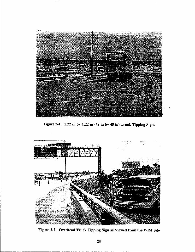
Figure 2-1. 1.22 m by 1.22 m (48 in by 48 in) Truck Tipping Signs
Figure 2-2. Overhead Truck Tipping Sign as Viewed from the WIlVl Site
20

Figure 2-3. Close-up of Overhead Sign
Figure 2-4. Static Signs with Active Flashing Lights
21

Figure 2-3. Close-up of Overhead Sign
Figure 2-4. Static Signs with Active Flashing Lights
21

vehicle must meet three criteria for the active lights to begin flashing. These are: 1) the vehicle must be tall enough to break the 2.16 m (7-ft I-in) beam, 2) it must be longer than the minimum length of 4.88 m (16 ft) at this height, and 3) its speed must be greater than the threshold speed entered by the user. The program logic which activated the lights also turned them off after 5 seconds.
Improvements to the active system included both software and hardware modifications. One software modification was needed for vehicles whose height was exactly 2.16 m (7-ft I-in). The most noticeable hardware improvement was the addition of a third infrared beam. The problem with the two-beam system was apparently related to the beam striking most trucks at windshield height. Apparently, a significant number of windshields were detected differently by the two beams. One beam might "see" the windshield but the other might not, giving erroneous results. To overcome the problem, the two-beam array was lowered so that its beams detected the metallic portion of the cab and the third (single) beam was positioned at the 2.16 m (7-ft I-in) height.
TTl installed a time-lapse video camera and video cassette recorder (VCR) at the cabinet location in April of 1993 in order to monitor the active system's performance. The camera's field of view included the active system's lights mounted near the first ramp curve. Upon arrival of a high-speed truck, the system controller generated two "alanns" -- one to initiate the lights and one to begin recording. The VCR was set to record 15 seconds for each actuation.
TTl installed a weigh-in-motion (WIM) system upstream of the ramp gore in lane one (the right-hand lane) to determine the correlation (if any) between truck weights on speeds. Figure 2-2 shows the WIM location in the foreground. This system used five temporary piezoelectric (TP) cable sensors similar to those used with the IRD classification system. Other hardware components of this system included an analog-to-digital board, a charge amplifier box, and a portable computer. The computer required expansion capability to accommodate the analog-todigital board, so not just any portable or laptop computer could be used. For the computer used in this study, a portable generator was also required. For future systems that integrate both classification and weight functions, it will be desirable to utilize a more compact, stand-alone, ruggedized computer system that can operate in an unmonitored mode for long periods of time.
DATA RETRIEVAL
A laptop computer provided the most convenient universal means of retrieving data from both of the traffic monitoring systems. Again, the WIM system required a special expandable computer. Factors considered important in connection with data storage and retrieval were: types of vehicles stored in memory, data elements stored for each detected vehicle, memory capacity, and sample size requirements. The CTR system had 32K bytes of memory, but it only stored vehicle number, hour, minute, second, length, and speed of trucks exceeding the dimensions noted earlier. The IRD system, on the other hand, contained 64K bytes of memory that were available for storing both cars and trucks. Data elements stored on each vehicle included: vehicle number, lane number, hour, minute, second, speed, and individual wheelbase spacings. In the raw data mode, the IRD software did not provide the option of eliminating cars.
22

The timing of data retrieval was based somewhat on availability of personnel traveling to the site, but more importantly, on the amount of available memory in each system. The CTR system I s memory was sufficient for several weeks of data storage, whereas the IRD system IS
memory would reach its capacity in less than 24 hours.
The initial data collection during the first few months of the project utilized a video camera to verify IRD results and to assist in the tracking process. Mter comparison of a few hours of IRD and video results, it was evident that the IRD system would provide data sufficiently accurate to track vehicles along the ramp. With increased confidence in the IRD results, video tracking was virtually eliminated during the remainder of the project.
Manually matching trucks at the three sites along the ramp from three different data sources was not difficult, but it was quite labor intensive. To expedite the process, a Foxbase computer program was written to read the raw data files and generate matched vehicle output. First, the Foxbase program eliminated small vehicles such as cars, motorcycles, and four-tire trucks from the sample. It also removed trucks following other vehicles at short headways in case these leading vehicles interfered with truck speeds. Then, trucks with recorded speeds much greater than or much less than reasonable speeds were considered as extreme outliers and were deleted from the sample. Data collected during inclement weather was not considered.
Collection of vehicle WIM data required an operator to remain with the monitoring system during the data collection period. The purpose of WIM data was to determine if speed reduction was correlated with the loading condition. This WIM system required the installation of five TP sensors on the pavement, and other equipment described above.
DATA ANALYSIS
The IRD files were the only ones that could be used to trace vehicles completely through the ramp and detect speed change under the various conditions. These files were larger than those from other sources, however, necessitating computerized assistance to handle the unwieldy matching tasks. The matching program traces vehicles from site A to site B to site C. It consists of three steps: 1) formatting the IRD files, 2) removing irrelevant vehicle records, and 3) matching pairs of files A and B with A and C.
Formatting the IRD Files
The first step in the formatting process was to convert IRD data files from Locations (parameter named "sites") A, B, and C into a format that could be read by the FoxBase database software used to process the files. This included removing the header of the file generated by the IRD equipment and any other extraneous information included in the file other than the vehicle (data) records. Figure 2-5 provides an example of the IRD file header.
23

lFile OPENED at 04/08/93 15:00 STORAGE: RAW ~ITE : 610/59 iINFO#1 : Loc. C iINFO#2 : 2d curve ~ Active Lanes. Date Format = MMIDDIYY. Unit Type = 5 1: LANE USED TRIG = TUBE AXLE = TUBE PRES = NONE
Sensor Spacing = 16.0' INFO: right lane 0 Record Intervals.
~: LANE USED TRIG = TUBE AXLE=TUBE PRES = NONE Sensor Spacing = 16.0'
~FO: Left lane 0 Record Intervals.
Figure 2-5. Example of an IRD File Header
The second step involved formatting the vehicle (data) records by removing any special characters like the (") character after the wheelbase length, or the "mph" characters after the speed field. Figure 2-6 is an example of records before formatting.
The next formatting step separated the fields from each other by one space and removed existing spaces before the first field in a record. Figure 2-7 demonstrates these formatted records.
This process used a text editor to convert (edit) the files. After the conversion was complete, the next step transferred formatted fIles from sites A, B, and C into the database files A.dbf, B.dbf, and C.dbf, respectively.
1: 15:01:13 53 mph, 2 Axles, 8.2' 2: 15:01:11 33 mph,S Axles, 18.6' 4.3' 29.0' 3.8' ~: 15:01:14 32 mph, 4 Axles, 8.0' 40.8' 9.4' ~: 15:01:17 92 mph, 2 Axles, 30.8'
Figure 2-6. Example of Records Before Formatting
1 15 01 13 53 2 8.2 ~ 150111 33 5 18.64.329.03.8 2 1501 143248.040.89.4 215011792230.8
Figure 2-7. Example of Records After Formatting
24

Removing Irrelevant Vehicle Records
Preprocessing of database flIes A, B, and C removed vehicles that were not relevant for this study. This fIrst classified the vehicles and moved the non-trucks into separate flIes. Second, the remaining vehicles in each fue that had headways of 2 seconds or less were removed because of possible interference by the leading vehicle.
Matching Pairs of Vehicles at A and B with A and C
The next step was to compare vehicles in ftle A with vehicles in ftles B and C. The criteria used to trace vehicles from Location A to Location B or C was based on the time needed for a truck to travel from Location A to the other sites with some reasonable tolerance. The allowable time for a vehicle to travel from A to B was 3 to 10 seconds, and the time allowed from A to C was between 17 and 40 seconds.
Also included in the tolerance criteria was the total length of the truck as calculated by the classifiers at each site. All three sites used piezo sensors in the beginning of the study. However, due to the high failure rate of TP sensors at Location A, an alternate system of permanent loops and piezos had to be used. In order to take into consideration the difference in total length between a vehicle measured by the loop detectors at Location A and the same vehicle measured by piezo sensors at Locations B and C, a tolerance ranging from 1.8 m to 3.4 m (6 to 11 ft) was allowed as the difference between total lengths of vehicles from Location A and Locations B or C. Inductive loops detect a different vehicle length than do piezo sensors. Vehicles in fue A that have matches in fues B or C, according to the above criteria, were placed in fues AB and AC, respectively. Figure 2-8 provides an example of the contents of output fue AB or AC.
~ 2 09 25 49 51 2339497.60 2 B 1 092552592339529.802 19920616 ~ 1 092653292340137.302 B 1 092703 60 2 34023 8.702 19920616 ~ 2 09270872 2 34028 11.703 B 10927 14552340348.702 19920616 ~ 2 09 27 087223402811.703 B 2 09 2715572340359.30219920616 ~ 1 092857 102341379.202 B 1 092902392341428.00 2 19920616 ~ 1 092857102341379.202 B 2 09 29 04 512 3414411.803 19920616 ~ 2 09 29 04 60 2341448.302 B 1 092911 4223415113.203 19920616 ~ 2092907642341479.302 B 1 092911 4223415113.203 19920616 ~ 2 09 30 19 55 2 34219 9.30 2 B 1 09 30 22 54 2 34222 7.80 2 19920616 ~ 1 09 30 37 312342377.202 B 1093045452342458.302 19920616 Al 09 30 56 26 2 34256 6.202 B 2 093105442342658.502 19920616 A209 31085223426811.103 B209 3113 53 2 342739.80219920616 Al 09 313027234290 7.90 2 B 2 09 3133512342939.502 19920616 Al 09 31 3027234290 7.90 2 B 2 0931374823429712.00 3 19920616 A 2 09 31 4462234304 10.90 3 B 1 0931 4949234309 12.503 19920616
Figure 2-8. Example of Output Files
25

Every record consisted of 21 fields. The first 10 fields were for the vehicle from Location A, while the next 10 fields were for the vehicle from B or C. The last field was the date field. Every vehicle set of fields consisted of the following from left to right: Location, Lane, Hour, Minute, Second, Speed, No. of Axles, Total Time in Seconds, Total Length, and Vehicle Class.
Tracing Vehicles from Site A to Site B to Site C
The next step compared records of vehicles in ftle AB with vehicle records in file AC. The records in both ftles that had the same vehicle A in common were considered as the same vehicle traced from A to B to C and were placed in a new file called ABC. Figure 2-9 is an example of the contents of the output file ABC.
The fields from left to right are: Lane, Hour, Minute, Second, Speed, No. of Axles, Site, Total Time in Seconds, Total Length, Vehicle Class, and Date. Every three consecutive records constitute a single vehicle traced from A to B to C.
For the last two steps, the program also had the capability of matching pairs of files A&B and B&C and then tracing a vehicle from sites A to B to C with vehicles in B as the common vehicle instead of matching with vehicles in A as the common vehicle for the records with pairs of vehicles.
21000 47 53.00 2 21000 54 46.00 2 2 10 01 09 54.00 2 2 10023260.00 2 2 10 02 35 44.00 2 210025457.00 2 2 10023260.00 2 2 10 02 35 44.00 2 1 10 0300 53.00 2 2 10023260.00 2 1 10 02 39 52.00 2 210025457.00 2
Statistical Analysis
A 36047 9.50 219920616 B 3605411.00 3 19920616 C 36069 8.402 19920616 A 36152 7.60 219920616 B 36155 9.40 219920616 C 36174 8.90 2 19920616 A 361527.60 219920616 B 36155 9.40 2 19920616 C 36180 11.90 3 19920616 A 361527.60 219920616 B 36159 8.802 19920616 C 36174 8.90 2 19920616
Figure 2-9. Example Data Set of Matched Vehicles
The computerized statistics package used to evaluate the speed and weight data was the Statistical Analysis System (SAS) (16). The process of evaluating truck speeds produced SAS programs designed to read the FoxBase output files and determine speeds and speed reductions among the three locations on the ramp. The PROC GLM and Duncan Multiple Range Test procedures generated sample means and the significance of differences among mean values and other parametric descriptors. Output generated by SAS was typically an evaluation of truck speed
26

reduction based on treatment type, vehicle speed at the ramp entrance, vehicle size/weight parameters, peak/off-peak conditions, day/night conditions, or interactions between two or more variables.
27


CHAPTER 3. LITERATURE REVIEW
INTRODUCTION
Several literature sources provided insight into the magnitude of large truck problems negotiating freeway curves. When Winkler et al. (11) evaluated the problem of truck stability, they frrst conducted a sUlvey of knowledgeable organizations to identify the sample set of vehicles thought most susceptible to exceeding acceptable stability performance limits. The survey included questions aimed at determining types of crashes considered most detrimental to the safety and mobility of the motoring pUblic. Responses from 29 states, four motor carriers, one trailer manufacturer, and the Brotherhood of Teamsters overwhelmingly concluded that rollover was the greatest concern, although yaw instability (often resulting in jackknife) was also regarded as highly problematic.
The Winkler study utilized Bureau of Motor Carrier Safety (BMCS) accident data for a three-year time period to determine the frequency of instability and handling problems. These data support the general conclusions of the survey; they show that 32 percent of the heavy (generally Class 7 and Class 8) vehicle accidents are classified as rollovers, while 18 percent are jackknifes. According to the data, jackknife is largely an empty-vehicle problem. Home (18) and Ivey (19) discovered an additional factor that can contribute to truck instability on wet pavements under lightly-loaded conditions. Truck tires can hydroplane where the depth of water and vehicle speed are sufficient to reduce tire contact with the pavement surface. For freeway connectors, this may become particularly troublesome for unloaded trucks on large-radius curves where combinations of high speeds, poor pavement friction, and/or poor drainage exist.
The growth in the number of trucks over the past several years has become a factor in their crash involvement. A study performed for the California Department of Transportation and documented by Reilly and Haven (20) indicated heavy truck percentages as high as 15 percent of total traffic on high volume urban freeways during off-peak periods. Findings of Middleton et al. (I) indicate truck volumes in excess of 25 percent of total traffic on segments of 1-5 north of Los Angeles and on 1-80/1-94 near Chicago. Besides reductions in pavement and bridge life, there are congestion and delay implications due to this growth in heavy truck volumes, especially when these trucks are involved in incidents or accidents. In a 1990 report, Roper (21) stated that truck accidents in California have increased by 10 percent per year since 1985 with delays averaging 2,500 vehicle-hours per accident.
GENERAL TRUCK CRASH STATISTICAL STUDIES
Studies of the involvement of large combination vehicles in crashes can be grouped into two categories: general statistical studies and explicit studies of crashes on freeway-to-freeway connectors. The first is used to investigate factors contributing to large truck crashes on a State or national level. The second method uses computer simulation to identify common factors found to influence similar crashes.
29

-- - ------------ ---------------------------l
Truck crashes on urban freeways occur predominantly at interchanges, with exit ramp crashes more frequent than entrance ramps. According to Vallete et al. (23.), as many as 21 percent of all truck accidents on urban freeways occur at interchanges. Two crash types, typically occurring on curved ramps and often associated with excessive speed and loss of control, are truck rollovers and jackknifes. Overturned truck crashes on exit ramps at interstate interchanges represent 5 out of every 100 fatal truck crashes.
Of the 11,069,000 vehicles estimated to have been involved in crashes in 1986, 235,000 (2.1 percent) were combination trucks. Even though this percentage is small, it should be noted that when combination vehicles are involved in crashes, there is typically an increase in severity. Of the 60,755 vehicles involved in fatal crashes in 1986, 6.7 percent were combination vehicles -three times the proportion involved in crashes (24). According to a 1991 report titled Trucks Involved in Fatal Accidents Factbook 1987 (25), trucks over 4,540 kg (10,000 lb) Gross Vehicle Weight Rating (GVWR) were involved in 41,187 fatal crashes throughout the U.S. from 1980 through 1987. This is an average of 5,148 fatal crash involvements per year. Of the total 5,275 fatal crashes in 1987 involving trucks, tractor-semitrailers were involved in 3,266 and doubles were involved in 232 fatal crashes.
Twenty-four percent of the 1987 fatal truck crashes occurred on limited access highways (25). Ervin et al. (26, Tl) cited Bureau of Motor Carrier crash data for 1980 showing that nine percent of all jackknife crashes and 16.8 percent of all truck rollover crashes occur on ramps. These percentages indicate that ramps are problematic, given that their crash percentages are significantly higher than the proportion of vehicle miles of travel on ramps compared to mainlanes.
Generic Studies of Truck Crashes
Recent statistical studies cited by Leonard and Recker (30) have identified factors that contribute to large truck crashes. These studies generally evaluate accident rates based on national accident statistics, using large scale databases such as FARS (Fatal Accident Reporting System), BMCS (Bureau of Motor Carrier Safety), NHTSA (National Highway Traffic Safety Administration), and NASS (National Accident Sampling System). These data are usually supplemented by individual state crash databases. Unfortunately, none of these large national databases identifies crashes occurring explicitly on freeway connectors; usually they include freeway-to-freeway connector data with ramp data. In some cases, all freeway data, including interchange data, are combined.
A recent NASS data set evaluated by Hilton and Meyer (3.1) indicated that the worst type of crash with respect to injury was rollover, and its significance was compounded by its frequency. From 1979 to 1986, rollover occurred in almost 14 percent of all single vehicle truck crashes, and it resulted in over 60 percent of the total truck occupant injuries. Of 4,640 single vehicle crashes (involving only heavy trucks) evaluated by first harmful event, 55 percent were "ran-off-road" type crashes, 17 percent were overturns, and 13 percent involved jackknifes. These were mutually exclusive categories.
30
I

Bowman and Hummer (22) examined truck crashes on urban freeways to determine their consequences as a function of vehicle type, traffic operations, and roadway characteristics. Their study was limited to high speed, high volume freeways that had a minimum of five percent trucks (over 4,540 kg [10,000 lb] GVWR). A total of 2,221 truck crashes occurred on five selected freeway segments whose lengths added together totalled 74.9 km (46.5 mi). These crashes covered a time period from January 1985 through September 1988. The study compared these truck crashes with 17,962 crashes occurring during the same time period and on the same segments, but involving only passenger cars. Fatality rates were higher for trucks: five persons were killed for each 1,000 accidents compared to 2.2 fatalities for autos only.
One of the few crash studies that actually examined accident rates (considered vehicle-miles traveled) in a manner that isolated urban freeways from other roadway types was conducted by McCasland and Stokes (32). This study found that on six Houston freeways the proportions of trucks involved in crashes was higher than the proportion of trucks on the freeways. Other fmdings included the fact that 18.5 percent of all crashes on freeway segments involved trucks, while 5.9 percent of the total traffic volume was trucks. Truck drivers were found to be not at fault in 50.4 percent of the crashes investigated. In crashes where truck drivers were cited as performing a hazardous action which led directly to the crash, the most common actions were: improper lane use (15.9 percent), following too close (13.6 percent), and speed too fast for conditions (8.1 percent). Improper lane use usually involved the truck driver changing to the lane to the right, striking a vehicle which already occupied that lane. Location of the crash was categorized as freeway proper, exit area, and merge area; 76.9 percent of the crashes investigated in this study occurred on the freeway proper. Freeway-to-freeway connectors were not separately considered.
Freeway Connector and Ramp Studies
Golob and Recker (29) used the discrete multivariate method of log-linear modeling to calculate indices of association between categories of variables. This method begins with a known distribution among types of crashes for all freeway segments and determines if there is significant interaction between route segment and collision type. Results were compared with the chi-square distribution for hypothesis testing. Analyses were divided into two categories: (a) accident characteristics by collision type and (b) accident characteristics by freeway route segment. The study analyzed accident data for 38 freeway segments in southern California using the California Department of Transportation (Caltrans) Traffic Accident Surveillance and Analysis (TASAS) database. More than 9,000 truck-involved crashes during the two-year time period from 1983 to 1984 provided the basis of the study.
Results of the study indicated that, at the p=0.05 level, there was strong association between collision type and accident location, roadway terrain, time period, road conditions, weather conditions, and surface conditions. The accident location analysis differentiated between highway and ramp locations, identifying overturns, broadsides, and hit-object crashes as those crash types occurring predominately on ramps.
31

In other research using the Caltrans TASAS database, Leonard and Recker (3.0) studied freeway connectors in California for the 8 112 year time period from January 1, 1979 through July 31, 1987. Their database utilized 1,745 crashes involving large combination vehicles on freewayto-freeway connectors in Los Angeles and Orange Counties.
Twenty-seven percent of the 1,745 crashes on connecters were the loss-of-control type. These 478 crashes can be broken down as follows: rollovers 35.8 percent and run-off-road 64.2 percent. The numbers of loss-of-control and all other truck-involved connector crashes increased at similar rates from 1979 through 1986. Least squares regression slopes for both of these categories were significantly different from zero at the p=0.05 level. Loss-of-control crashes increased at approximately nine percent per year, while all other crashes increased at approximately seven percent per year.
Leonard and Recker (3.0) reported that among several causal factors related to loss-ofcontrol, speeding was the most highly significant (p < 0.001). Speedjng was a factor jn 68 6 percent of a]] loss-of-contmlcrashes, whereas "other violations" were 10.7 percent, "not driver" was 9.2 percent, "improper tum" was 7.7 percent, and "other" was 3.8 percent. Furthennore, the analysis found that speeding was a factor in 78 percent of the 17 connectors (of the total 200) with the highest number of truck crashes. Next, study fmdings indicated that loss-of-control crashes were more severe than the "other" category, resulting in injuries or fatalities 45.2 percent of the time, compared to 20.3 percent for non-Ioss-of-control crashes.
SIMULATION STUDIES OF TRUCK CRASHES
Recent studies (TI, 26, 28, 3.0, 33, 34, 35) have utilized the PHASE4 simulation model (36) to study loss-of-control crashes involving appropriate AASHTO design vehicles on freewayto-freeway connectors. PHASE4 is a computerized model for simulating the braking and steering dynamics of large trucks, tractor-semitrailers, doubles, and triples combinations. The University of Michigan Transportation Research Institute (UMTRI) developed the model under the sponsorship of the (then) Motor Vehicle Manufacturers Association (MVMA) and the Federal Highway Administration (FHW A).
The modeling process must consider that, in the context of negotiating horizontal curves, commercial vehicles are subject to two general classes of instability, namely divergent roll response (rollover), and divergent yaw response (spin-out or for articulated vehicles, jackknife). Another class of instability, particularly in multiply-articulated combination vehicles, sometimes referred to as rearward amplification, was not included due to nonapplicability.
The maximum lateral acceleration that a vehicle can sustain without tipping over is, by definition, its rollover threshold. According to Ervin et al. (35), the rollover threshold for heavy trucks can be as low as 0.27 g, whereas McGee found that passenger cars have rollover thresholds of approximately 1.20 g. This means that passenger cars can sustain more lateral acceleration than trucks without rolling over. In fact, cars will generally begin to skid at their maximum lateral acceleration instead of rolling over.
32

Winkler et al. (U) describe the nature of yaw instability for heavy trucks as a slow, continuous build-up of lateral acceleration by the vehicle for a fIxed steering wheel input. That means that the vehicle will tum, not on a perfect circular arc, but on a tighter and tighter spiral. This tighter turning behavior leads to increased lateral acceleration levels until rollover occurs. This yaw instability can occur in high c.g. commercial vehicles during moderate turning maneuvers (0.2 to 0.3 g) while operating at highway speeds. For lightly loaded or unloaded commercial vehicles on slick pavements, yaw instability may result in loss of control without rollover as the tractor rotates rapidly into the trailer.
The simulation process incorporates both the detailed operating characteristics of specifIc design vehicles that use the highways and the as-built features of the roadway. To a lesser extent, it includes characteristics of drivers who operate those vehicles. Vehicle characteristics used in highway design and operational considerations change continually as a result of changes in size and weight laws and performance enhancements such as increased horsepower-to-weight ratio and moveable trailer axles. These vehicle-specifIc and driver population characteristics are critical inputs in the simulation process.
The first of the studies conducted by Ervin et al. (26), used simulation to examine relationships between roadway geometrics and truck safety at freeway interchanges. This study was apparently the fIrst of its kind to use an in-depth methodology to evaluate the effects of roadway geometrics on particular vehicle types. The study considered the influence of ramp geometry through direct simulation of vehicle response on geometrics that replicate the as-built design of the roadway. The Ervin study used single-unit or combination vehicles with class 7 or class 8 power units -- those with Gross Vehicle Weight Ratings (GVWR) of over 11,804 kg (26,000Ib).
The study began with national crash data from the Bureau of Motor Carrier Safety (BMCS), Fatal Accident Reporting System (FARS), National Accident Sampling System (NASS), and National Highway TraffIc Safety Administration (NHTSA) databases to identify states with signifIcant numbers of truck crashes. Then, details on the ramps and the accidents were requested from the states to identify ramps to be used. Case studies used the following selection criteria: completeness of detailed crash information, availability of geometric design data, and prior crash history, especially concentrating on loss-of-control crashes. The lack of sufficient exposure data prevented researchers from using accident rates as one of the criteria. Special emphasis was placed on sites in which "loss of control" was a factor in the crashes. The criteria resulted in a total of 15 crash sites using 11 different interchanges in California, Illinois, Maryland, Michigan, and Ohio for detailed evaluation. The study used the PHASE4 model to simulate the dynamic responses of heavy vehicles negotiating case study interchanges.
During the simulation phase, Ervin used the PHASE4 model to simulate two loading configurations on a tractor-semitrailer vehicle: (a) a baseline loading that placed the payload center-of-gravity (c.g.) at 2.1 m (83 in) above the ground and (b) a loading condition with the payload c.g. at 2.7 m (105 in) above the ground. The first height was thought to characterize a large proportion of existing truck loading conditions, while the second height represented specialized tank vehicles and van trailers carrying a full cube load of homogeneous freight. The
33

vehicle used in the simulations was a cab-over-engine tractor with a wheelbase of 3.7 m (144 in) pulling a 13.7 m (45 ft) van-type semitrailer. The computer simulations varied the combination vehicle's speed, using the connector's advisory speed in some cases and in others, speeds greater than the posted advisory.
The five case studies developed by the Ervin study illustrated the more significant aspects of geometric design that limited margins of safety for heavy trucks operating on freeway connectors and ramps. Both the physical size of trucks and limitations in their physical performance caused problems when negotiating connector roadways. The five case studies are instructive due to their value in portraying truck instability problems on freeway connectors. They are:
• Case 1-- side friction factor is excessive given the roll stability limits of many trucks,
• Case 2 -- truckers assume that the ramp advisory speed does not apply to all curves on the ramp,
• Case 3 -- deceleration lane lengths are deficient for trucks, resulting in excessive speeds at the entrance of sharply curved ramps,
• Case 4 -- lightly loaded truck tires are sensitive to pavement texture in avoiding hydroplaning on high-speed ramps, and
• Case 5 -- curbs placed on the outer side of curved ramps pose a peculiar obstacle that may trip and overturn articulated truck combinations.
TRUCK FAILURE MODES
Failure modes for large commercial vehicles on freeway ramps and connectors typically include divergent yaw response and divergent roll response. A third failure mode, referred to as lightly damped, oscillatory yaw response -- rearward amplification, predominates in multiplyarticulated combination vehicles in evasive maneuvers where steering input is necessary for collision avoidance. This is not often found to be a problem on freeway connectors, so rearward amplification will not be considered in detail in this discussion.
Solutions to divergent yaw response crashes emerge as those requiring design and/or maintenance improvements to the roadway. For example, jackknifes often occur under conditions of wet pavements, reduced pavement friction, lightly loaded or unloaded vehicles, short deceleration lanes, and high approach speeds as on exit ramps approaching restrictive curvature. Therefore, this discussion will focus on the rollover phenomenon.
To conduct a comprehensive analysis of the rollover phenomenon, one must consider several vehicle parameters. Included are height, width, suspension geometry, and compliances of the body, suspension, and tires. It should be realized that the actual mechanics of the quasi-
34

static rollover process are rather complex and are usually highly non-linear. Considerable discussion of this complex rollover process can be found in the literature (11, 3.6, 31).
In the absence of computerized simulation, the method used to evaluate divergent roll or yaw response in heavy trucks assumes a simple point mass moving in a circular arc in a horizontal plane. Additional detailed information is available in the literature to facilitate a better understanding of various dimensional and mechanical properties of heavy trucks and how they affect rollover.
An advantage of the point mass assumption is its simplicity, but a disadvantage is its lack of distinction by vehicle type. However, this concern is addressed by utilizing additional tirepavement friction and rollover threshold data that allow prediction of stability limits in roll and yaw with reasonable accuracy (38). For this reason and because the point mass assumption is used by the AASHTO Green Book (1), the basis for its inclusion in this document is axiomatic. It should be noted that the point mass method does not provide a complete analysis technique for loads that shift.
A vehicle traveling along a level circular path of constant radius without superelevation has three principal forces acting upon it: 1) the force of gravity (or the vehicle's weight, W) which is considered to act through the vehicle's center of gravity, c.g., 2) the upward force, N, of the pavement which supports the vehicle and is equal in magnitude and opposite in direction to the vehicle's weight, and 3) the lateral force between the pavement and tires which counteracts the centrifugal force. There remains an unbalanced (centrifugal) force acting through the vehicle's center of gravity and whose direction is horizontal, pointed radially outward away from the cUlve's center. Compensation for this unbalanced centrifugal force usually comes, at least in part, from pavement superelevation.
For purposes of this discussion, the following assumptions apply: 1) the vehicle is considered to be a point mass, 2) the angular speed of the vehicle is constant, 3) the path of the vehicle in the tangential direction is level, 4) the vehicle is approaching a rollover condition (the normal force of the pavement is acting solely on the outside tire), and 5) the radius of the path traversed by the vehicle is equal to the radius of highway curvature.
Equation (1) shows the relationship used by AASHTO for calculating the side friction factor based on design speed, "V," curve radius, "R," and superelevation, "e." On a superelevated curve, the superelevation offsets a portion of the lateral acceleration and the tire/pavement friction resists the tendency of the vehicle to skid off the roadway.
v 2
f·---e 15 R
(1)
35
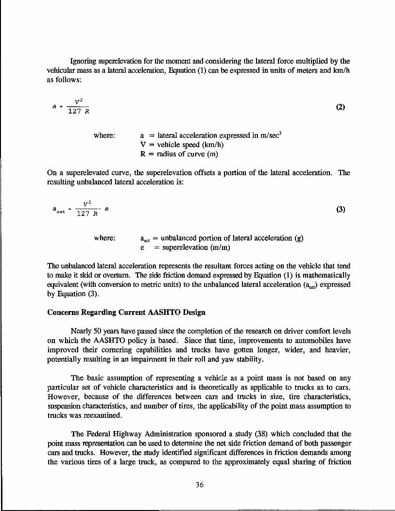
Ignoring superelevation for the moment and considering the lateral force multiplied by the vehicular mass as a lateral acceleration, Equation (1) can be expressed in units of meters and km/h as follows:
v 2 a • - ___ -
127 R
where: a = lateral acceleration expressed in ml sec2
V = vehicle speed (km/h) R = radius of curve (m)
(2)
On a superelevated curve, the superelevation offsets a portion of the lateral acceleration. The resulting unbalanced lateral acceleration is:
a • ---- e net 127 R
where: 3net = unbalanced portion of lateral acceleration (g) e = superelevation (m/m)
(3)
The unbalanced lateral acceleration represents the resultant forces acting on the vehicle that tend to make it skid or overturn. The side friction demand expressed by Equation (1) is mathematically equivalent (with conversion to metric units) to the unbalanced lateral acceleration (3neJ expressed by Equation (3).
Concerns Regarding Current AASHTO Design
Nearly 50 years have passed since the completion of the research on driver comfort levels on which the AASHTO policy is based. Since that time, improvements to automobiles have improved their cornering capabilities and trucks have gotten longer, wider, and heavier, potentially resulting in an impairment in their roll and yaw stability.
The basic assumption of representing a vehicle as a point mass is not based on any particular set of vehicle characteristics and is theoretically as applicable to trucks as to cars. However, because of the differences between cars and trucks in size, tire characteristics, suspension characteristics, and number of tires, the applicability of the point mass assumption to trucks was reexamined.
The Federal Highway Administration sponsored a study (3.&) which concluded that the point mass representation can be used to determine the net side friction demand of both passenger cars and trucks. However, the study identified significant differences in friction demands among the various tires of a large truck, as compared to the approximately equal sharing of friction
36

demands among the four tires of a passenger car. The net result of this variation is approximately 10 percent higher side friction demand in trucks than passenger cars. Additionally, truck tire rubber is harder than the rubber used for passenger car tires, reducing its tractive capability to 70 percent of automobile tire values.
Another inherent weakness in the point mass representation thus far has been no consideration of driver input as the vehicle negotiates the curve. In reality, as shown by field studies, all vehicles oversteer at some point on a horizontal curve (18). At the point of oversteering, the vehicle is following a radius that is less than the nominal curve radius. Thus, there is a high probability of the friction demand being greater in magnitude than that suggested by Equation (3). The AASHTO design policy does not consider oversteering by passenger cars but it may not be critical because the maximum lateral acceleration criteria are based on driver comfort levels rather than on available pavement friction. Later sections of this document·discuss corrections for oversteering and differences in tire friction.
Several authors have expressed concerns that side friction factors designed for discomfort ranges for passenger car occupants must be reevaluated in relation to implications for vehicles with relatively poor stability characteristics. These vehicles include large commercial vehicles with high centers of gravity. Weinberg and Thatp (39) expressed concern that the range of "f" values recommended by AASHTO fail to take into account the overturning tendency of a vehicle in a turn. Whiteside (40) pointed out that a side friction factor which has not exceeded the passenger car "driver comfort" range may be of sufficient magnitude to cause a heavily loaded vehicle with a high center of gravity to overturn while negotiating a horizontal curve. Harwood and Mason (41) used AASHTO criteria to compute margins of safety against skidding and rollover for cars and trucks on horizontal curves. Green Book (1) Tables ill-6 and ill-17 form the basis of their analyses. Their conclusions and recommendations for high-speed design include the following:
• The margins of safety against skidding and rollover appear to be adequate for trucks that do not exceed the high-speed (rural) design speed for curves designed in accordance with Table ill -6 of the Green Book.
• Minimum radius curves designed in accordance with AASHTO high-speed policy provide an adequate margin of safety against both skidding and rollover for passenger cars.
• Varying the methods for developing superelevation on horizontal curves has a modest effect on the likelihood of skidding or rollover by trucks.
• On horizontal curves with lower design speeds that are designed in accordance with Table ill-6, the most unstable trucks can roll over when traveling as little as 8 to 16 km/h (5 to 10 mi/h) over the design speed. This is a particular concern on freeway ramps, many of which have unrealistically low design speeds in comparison to mainlanes.
Based on these results, Harwood and Mason (41) do not recommend modifications of Table
37
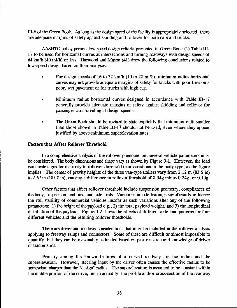
ill-6 of the Green Book. As long as the design speed of the facility is appropriately selected, there are adequate margins of safety against skidding and rollover for both cars and trucks.
AASHTO policy pennits low-speed design criteria presented in Green Book (1) Table ill-17 to be used for horizontal curves at intersections and turning roadways with design speeds of 64 km/h (40 mi/h) or less. Harwood and Mason (41) drew the following conclusions related to low-speed design based on their analyses:
• For design speeds of 16 to 32 km/h (10 to 20 mi/h), minimum radius horizontal curves may not provide adequate margins of safety for trucks with poor tires on a poor, wet pavement or for trucks with high c.g.
• Minimum radius horizontal curves designed in accordance with Table ill -17 generally provide adequate margins of safety against skidding and rollover for passenger cars traveling at design speeds.
• The Green Book should be revised to state explicitly that minimum radii smaller than those shown in Table ill-17 should not be used, even where they appear justified by above-minimum superelevation rates.
Factors that Affect Rollover Threshold
In a comprehensive analysis of the rollover phenomenon, several vehicle parameters must be considered. The body dimensions and shape vary as shown by Figure 3-1. However, the load can create a greater disparity in rollover threshold than variations in the body type, as the figure implies. The center of gravity heights of the three van-type trailers vary from 2.12 m (83.5 in) to 2.67 m (105.0 in), causing a difference in rollover threshold of 0.34g minus 0.24g, or 0.10g.
Other factors that affect rollover threshold include suspension geometry, compliances of the body, suspension, and tires, and axle loads. Variations in axle loadings significantly influence the roll stability of commercial vehicles insofar as such variations alter any of the following parameters: 1) the height of the payload c.g., 2) the total payload weight, and 3) the longitudinal distribution of the payload. Figure 3-2 shows the effects of different axle load patterns for four different vehicles and the resulting rollover thresholds.
There are driver and roadway considerations that must be included in the rollover analysis applying to freeway ramps and connectors. Some of these are difficult or almost impossible to quantify, but they can be reasonably estimated based on past research and knowledge of driver characteristics.
Primary among the known features of a curved roadway are the radius and the superelevation. However, steering input by the driver often causes the effective radius to be somewhat shatper than the "design" radius. The superelevation is assumed to be constant within the middle portion of the curve, but in actuality, the proftle and/or cross-section of the roadway
38

CASE CONFIGURATION
A. -r- Fun Gr .... Medium· OonsHy
"sAS!LINE" Freight 1!41blfl'l
':.r:: 00=00 "Typical" LT\. Froi9ht \.oDd
00=00 C. Full GroI'.
Full Cube, "HIGH .. CG" Homogeneous
Frei9ht (18.7 Ib/ll')
O· D. t e F.UGr ... 1"" -1- GoaoNne eer 00=00 T_
E. o Cry.v ..... Tonker
. (Ho, ond H,I
DAD
WEIGHT (lbsl
GVW
80,000
73,000
80,000
80.000
80,000
PAYLOAD CG ROLLOVER HEIGHT 'IliRESHOLO Onl (v"l
83.5 .34
95.0 .28
105.0 .24
88.6 .32
100. .26
t lb.' .4~~ tin .•. 02~4 m
• I IbllI" 16.01 ~/",'
Figure 3-1. Rollover Threshold Values for Various Example Vehicles
Vehicles I Case I Axle Number
A
~ 1 2 ._------!!
~18j I 2 :3
f-
~27=a I 2 :3
D
b!t;=45' Od I 2 :3 45
Axle Loods/lCXX>lb ROLLOVER THRESHOLD.9'S
I 2 3
12 18 12 20 12 22 12 24
12 16 16 12 17 17 12 18 18 12 19 19
lO 17.5 17.5 10.5 18 18 10.5 20 20 10.5 22 22
10.5 24 24
9.3 16 16 10 17.5 17.5 12 17 17 10 20 20 12 19 19
4
16 17.5 17 19 19
5 .200 .?J:1J 4 00
~ 7
~ I 1$
O-f-- 7 ~
/ 16 ~ 17.5 17 0--- -:t. 19 r 19
o Payload C.G. Height-tOO" (Cube-fuJI Load)
6. Payload C.G. Height Varies with Gress WeightMedian Density Freight.
Figure 3-2. Influence of Axle Load Variations on Rollover Threshold
39

can be altered at any location by overlays, pavement rutting, potholes, and environmentally induced surface undulations. Based on these and perhaps other esoteric factors that can influence the stability of trucks negotiating freeway connectors and ramps, it was suggested by McGee et aI. (42) that a safety margin be considered and that an allowance be made for steering fluctuations. The steering fluctuation factor would reduce the maximum lateral acceleration by 15 percent as proposed by Ervin et al. (26). Equation (4) is the resulting expression for the maximum lateral acceleration based on the rollover threshold of the truck.
RT - SM a
Ymax 1.15
where: ~ max = Safe lateral acceleration RT = Rollover threshold SM = Safety margin
(4)
According to Ervin et al. (35), there are other factors that could have at least a modest impact on rollover threshold. A few of these that have been quantified through simulation include vehicle width, weight distribution front to back, and differences between double and single trailer combinations. Four vehicle width parameters influence vehicle rollover: width of the trailer body, width between trailer tires, width between spring centers, and tractor width. Of these four, a wider tractor (2.4 m to 2.6 m [96 in to 102 in]) has the greatest impact in reducing rollover threshold and all four together would increase the rollover threshold by approximately 0.03 g.
The distribution of weight from front to back, or vise versa, has a minimal effect on rollover threshold. Shifting toward the front of the trailer is worse than shifting toward the rear, but even this reduction is only approximately 0.01 g. For the same width, weight, and c.g. height, double trailer combinations consistently have rollover thresholds 0.03 g to 0.05 g higher than tractor-semitrailers. Therefore, the latter are of the greater concern.
Rollover Threshold for Design
Ervin et al. (35) suggest that a rollover threshold of 0.30 g is appropriate for design PUIposeS, even though the worst case tractor-semitrailer exhibited a rollover threshold of 0.27 g if differences between simulation and reality are considered. Assuming the widespread use of wider (2.6 m [102 in]) trailers increases the design value by another 0.03 g. Therefore, the most unstable loaded truck could be expected to exhibit a rollover threshold of 0.30 g. In a more realistic sense, commonly accepted design practice is to use, not the worst case, but perhaps the 85th percentile. This is approximately 0.40 g, so horizontal curve design based on 0.30 g would be conservative.
40

CHAPTER 4. DRIVER CONSIDERATIONS
INTRODUCTION
According to the Tri-Level Study of the Causes of Accidents as cited in Reference (43), there is a direct correlation between driver errors and accidents. This study conducted an in-depth analysis of driver factors involved in 353 accidents to identify driver errors that contributed to the accidents. The study utilizes a model which breaks the driver decision pattern into its possible elements, beginning with the first contributing error, and following through subsequent compounding errors until the accident occurred.
Using this methodology resulted in an aggregated total of between 56 and 94 percent of the study accidents that were precipitated by human error. Driver recognition errors were cited as factors in between 27 and 41 percent of the accidents. The report provides aggregate totals for the two categories "recognition error" and "highway related environmental factors" (e.g. inadequate signs and view obstructions). The total number of accidents within these two categories which fell into the classification of "definite cause" was 56 percent. Adding "probable cause" accidents within these two categories to "definite cause" resulted in a total 94 percent of the accidents that were initiated by human error.
HUMAN FACTORS
Human factors assumptions currently prevalent in the design of roadways must be considered to appreciate the effectiveness of traffic control devices placed along the roadway. Although some of the human characteristics contained in the AASHTO Green Book (1) are qualitative, others are quantitative. An example of qualitative criteria is "driver comfort" on horizontal and vertical curvature. Quantitative criteria include perception-reaction time and driver eye height. The following discussion of human factors includes these and other important criteria promulgated in a recent task force effort (43) and earlier research efforts initiating the concept of Positive Guidance (44).
Because the driving task requires receiving and using information, it is important to ensure efficient communications and to make the message credible. An understanding of information use is critical to those who are responsible for ensuring a reasonably safe roadway environment. The fact that 90 to 95 percent of the information motorists need to drive safely is received visually (45) clearly tells the highway engineer that traffic control devices are essentially a visual information system. This visual information must be available to the driver during all weather and lighting conditions and should contain sufficient consistency and redundancy through shape, color, size, and message content so as to reinforce its message.
Driver Comfort Levels
The Green Book promulgates horizontal and vertical curve design based on "comfort levels" of vehicle occupants. Chapter III of this document provides additional details on the design of horizontal curves. The Green Book's guidelines on vertical curves requires that the rate of change of grade be kept within "tolerable limits," suggesting that sag vertical curves are more critical for comfort than crest due to centrifugal force and gravitational force acting in the same direction.
41

Establishing comfortable limits on horizontal curves has been done for many years by using a ball bank indicator. This device consists of a steel ball in a curved glass tube that is filled with a liquid. The ball is free to move inside the tube except for the damping effect of the liquid. Printed graduations on the curved tube provide information on the lateral acceleration applied to the vehicle. Taking into account the superelevation and the vehicle's body roll, one can set advisory speeds on a horizontal curve according to established criteria. These criteria, established approximately 50 years ago by Moyer and Berry (46), result in the side friction factors shown by Table 4-1. Other values of side friction factors became available as prevailing speeds increased; the Green Book values for design speeds of 97 kmlh (60 rnilh) and 113 kmlh (70 rnilh) are 0.12 and 0.10, respectively.
Texas Department of Transportation (TxDOT) engineers checked the advisory speeds on the I-61OIUS-59 connector using the ball-bank indicator method a short time before this research began. The resulting advisory speeds posted on the curves were 40 kmlh (25 rnilh) on the first curve and 56 kmlh (35 rnilh) on the second curve.
Table 4-1. Comfortable Horizontal Curve Criteria
Speed Range Ball-bank Readings (kmlh) (degrees) Side Friction Factor
~ 32 14 0.21
40 and 48 12 0.18
56 thru 80 10 0.15
Human Factors Considerations on Freeway Connectors
Because of typically lower design speeds on freeway connectors as compared to mainianes, the potential exists for unsafe speeds, especially on exit ramps. Failure modes in large trucks are often exhibited as divergent yaw response or divergent roll response. Either of these failure modes typically yields catastrophic results based on debilitating injuries, property damage, cargo spillage, and long delays to other freeway motorists. Most truck drivers are highly skilled, conscientious professionals, who are generally aware of these safety implications; however, many of them also have incentives to travel at relatively high speeds. These incentives include being compensated (in some cases) based on the number of payload units and/or the number of trips per unit of time and the difficulty, if going slow, of merging with high speed freeway traffic.
In considering where the signs should be placed on the connector roadway, TxDOT personnel hoped to utilize existing sign supports, but checking available reaction times based on prevailing speeds was important for obvious reasons. The following human factors rationale was used to check these locations; the static "ground-mounted" signs near Location B serve as examples.
First, reasonable deceleration rates are important, especially to truck drivers, because of the relatively low stability thresholds of their vehicles. Inherent in this discussion is providing the proper
42

warning sufficiently in advance of the hazard to allow perception and reaction time and a reasonable deceleration distance. Ervin et al. (26) used a deceleration rate of 0.16 g as a reasonable deceleration limit for wet or dry conditions in evaluations of deceleration lane lengths. This equates to 1.6 m/ sec2
(5.2 ftlsec~. The Green Book implicitly uses a 0.13 g deceleration rate in Table X-6 to compute the minimum deceleration length for vehicles exiting the mainlanes at an average running speed of 90 kmlh (55 milh) and decelerating to a speed of71 kmlh (44 milh) in a distance of85 m (280 feet). (These speeds closely replicate the I-610/US-59 average running speeds at Location A and Location B.) Some of the implied deceleration rates in Table X-6 exceed the 0.16 g value used by Ervin et al.; the value of 0.16 g will be used in the analysis to follow.
Figure 1-2 in Chapter 1 shows the position of the first set of warning signs near Location B. These signs were located 37 m (120 ft) upstream of the first curve's point of curvature (PC), the PC being the location of the piezo sensors on both curves. As the figure shows, the distance from the beginning of the ramp to the PC of the first curve was 243 m (797 ft). Once truck drivers reached this point on the curve, their line of sight was unobstructed (except possibly by tall vehicles in front ofthem) to one or both of the truck tipping signs near the first curve.
Assuming a perception-reaction time of 2.5 seconds (Green Book value) and an 85th percentile truck speed at Location A of 95 kmlh (59 milh), trucks would hypothetically begin decelerating after traveling at a constant speed of95 kmlh (59 milh) for 2.5 seconds (say 67 m [220 ft]) at which point the driver would be 9 m (30 ft) from the signs. So, the driver would still be 90 m (150 ft) from the PC of the 2 degree curve and 76.2 m (250 ft) from the PCC of the 7 degree curve. The deceleration rate will utilize this full distance because rollover potential would not be great within this flat portion of the curve. If truck drivers had actually decelerated to the posted advisory speed of 40 km/h (25 mi/h), the implied 85th percentile constant deceleration rate would be 0.38 g, or much higher than desired. In reality, the 10th percentile speed measured during the study at Location B was 65 kmlh (40 mi/h) and the very slowest trucks were traveling at 55 kmlh (34 milh), indicating that no trucks slowed to 40 kmlh (25 milh).
The plot of these actual ramp data closely resemble the Normal Probability Distribution Function. Fundamental properties of the Standard Normal Distribution (SND) include its plotted symmetrical shape centered about the sample mean and the area under its curve. This sample shows a mean speed reduction of 10 km/h (5.9 mi/h) and a standard deviation of 5.3 kmlh (3.3 milh). Based on the known characteristics of the SND, there is an 85 percent probability that the speed reduction will not exceed 1.5 standard deviations above the mean value. This 18 kmlh (11 milh) change implies an actual constant maximum deceleration rate of 1.55 m/sec2 (5.09 ftl sec2
) or 0.16g. This finding is informative from two perspectives: the driver's perspective and the highway
engineer's perspective. The 85th percentile truck driver's deceleration rate appears to agree with the limits used by Ervin as cited above, although it exceeds the cited example value from the Green Book. From the highway engineer's perspective, no apparent need existed to decelerate to the posted advisory speed value of 40 kmlh (25 milh) on the first curve. This suggests that rethinking the "comfort levels" currently used for horizontal curve design might be in order (assuming that 40 km/h [25 mi/h] was accurately determined). If truck drivers were ignoring these advisory speeds, drivers of passenger cars must have found them even less meaningful. A thorough evaluation of the effectiveness of the traffic control methods used on this connector will be provided in Chapter 5.
43

Similar logic to that used above applies to the second set of "ground-mounted" static signs near Location C and to the overhead sign. Both locations utilized existing sign mounting hardware as much as possible. The overhead sign's lateral location was directly over the right-hand exiting lanes (see Figure 2-2) so that drivers would be more likely to associate it with the ramp than with mainlanes.
TRUCK DRIVER INTERVIEWS
This section reports on two sets of truck driver interviews designed to determine the most effective warning devices for hazardous locations. The first interviews, which occurred as part of a study sponsored by the Federal Highway Administration (2), occurred generally at truck stops in Maryland and Virginia. The second set occurred in Texas during the initial phase of the 1-61O/US-59 project in early 1992.
Driver Interviews in Maryland and Virginia
A recent study by Knoblauch and Nitzburg (2) addressed human factors involved with truck driver warning signs in advance of potential rollover hazards. One of their early tasks resulted in a survey of 15 states to identify traffic control devices used at interchange ramps with histories of rollover accidents. Many of the states used variations of the standard MUTCD traffic control devices; others increased the size and/or number of devices or attempted innovative approaches at known problem locations. Survey results are provided in Chapter 1.
The first session of truck driver interviews, which occurred at a truck stop in Maryland, solicited opinions from 61 truck drivers regarding the effectiveness of existing signing and allowed them to design their own signs. The three general questions asked to all truck drivers were: 1) What information about a hazardous ramp is essential to truck drivers pulling a "top heavy" load, 2) How can signs be made to be more understandable, and 3) How can signs be made to be more believable to drivers.
Responses from professional truck drivers on question 1 included their ranking of which ones were most important. Recommended speed, degree of sharpness of the curve, and superelevation were of prime importance. Subordinate to these were: curve direction, curve length, and traffic control (if any) at the end of the ramp.
Question 2 results were also informative, although somewhat puzzling. To make signs more understandable, 21 drivers said add flashing lights, 17 said use multiple signs with considerable advance placement, 12 thought a symbol or illustration of a truck rolling over would be most understandable, 9 thought large printed words would best communicate a warning, and five stated that much larger than normal size signs should be used. The interpretation of some of these results, especially the 21 drivers who recommended flashing lights to "increase understanding," suggests either a lack of understanding of the question or misinterpretation by the interviewer.
Question 3 responses, regarding making the device believable to drivers, were somewhat similar to question 2 responses, suggesting that perhaps some of the truck drivers interviewed define "understandable" and "believable" synonymously. Driver responses on how to make signs believable
44
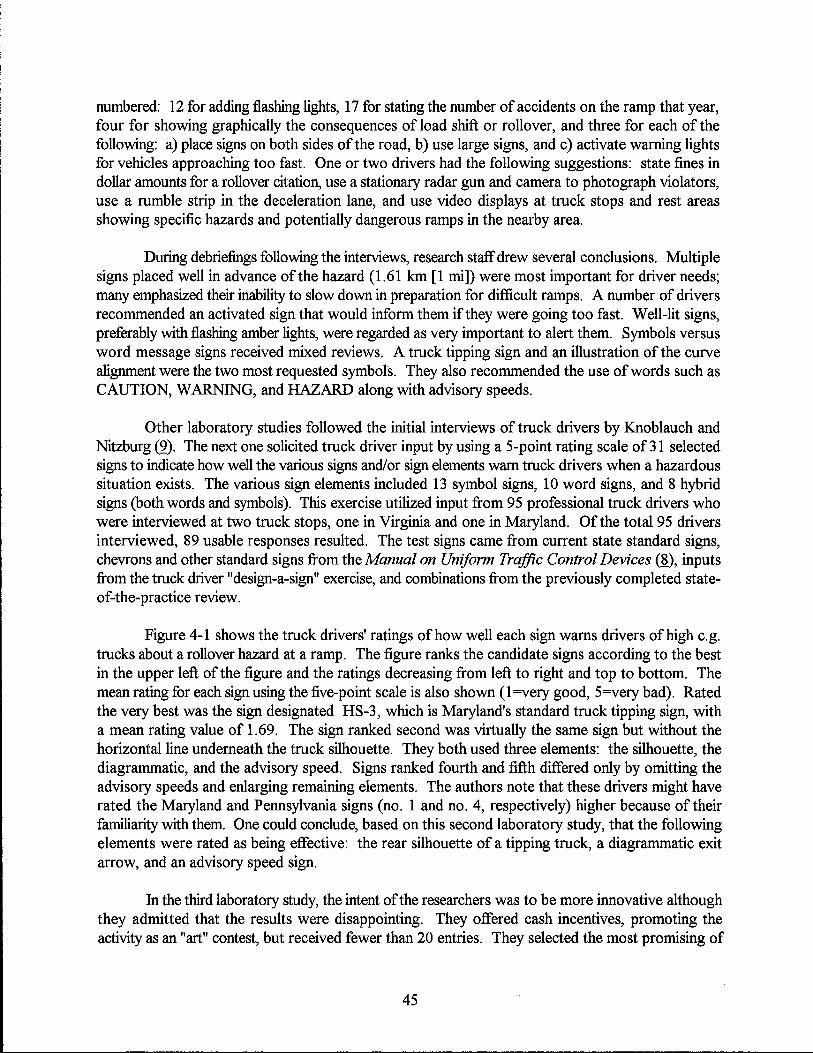
numbered: 12 for adding flashing lights, 17 for stating the number of accidents on the ramp that year, four for showing graphically the consequences of load shift or rollover, and three for each of the following: a) place signs on both sides of the road, b) use large signs, and c) activate warning lights for vehicles approaching too fast. One or two drivers had the following suggestions: state fines in dollar amounts for a rollover citation, use a stationary radar gun and camera to photograph violators, use a rumble strip in the deceleration lane, and use video displays at truck stops and rest areas showing specific hazards and potentially dangerous ramps in the nearby area.
During debriefings following the interviews, research staff drew several conclusions. Multiple signs placed well in advance of the hazard (1.61 km [1 miD were most important for driver needs; many emphasized their inability to slow down in preparation for difficult ramps. A number of drivers recommended an activated sign that would inform them if they were going too fast. Well-lit signs, preferably with flashing amber lights, were regarded as very important to alert them. Symbols versus word message signs received mixed reviews. A truck tipping sign and an illustration of the curve alignment were the two most requested symbols. They also recommended the use of words such as CAUTION, WARNING, and HAZARD along with advisory speeds.
Other laboratory studies followed the initial interviews of truck drivers by Knoblauch and Nitzburg (2). The next one solicited truck driver input by using a 5-point rating scale of 31 selected signs to indicate how well the various signs and/or sign elements warn truck drivers when a hazardous situation exists. The various sign elements included 13 symbol signs, 10 word signs, and 8 hybrid signs (both words and symbols). This exercise utilized input from 95 professional truck drivers who were interviewed at two truck stops, one in Virginia and one in Maryland. Of the total 95 drivers interviewed, 89 usable responses resulted. The test signs came from current state standard signs, chevrons and other standard signs from the Manual on Uniform Traffic Control Devices (~), inputs from the truck driver "design-a-sign" exercise, and combinations from the previously completed stateof-the-practice review.
Figure 4-1 shows the truck drivers' ratings of how well each sign warns drivers of high c.g. trucks about a rollover hazard at a ramp. The figure ranks the candidate signs according to the best in the upper left of the figure and the ratings decreasing from left to right and top to bottom. The mean rating for each sign using the five-point scale is also shown (1 =very good, 5=very bad). Rated the very best was the sign designated HS-3, which is Maryland's standard truck tipping sign, with a mean rating value of 1.69. The sign ranked second was virtually the same sign but without the horizontal line underneath the truck silhouette. They both used three elements: the silhouette, the diagrammatic, and the advisory speed. Signs ranked fourth and fifth differed only by omitting the advisory speeds and enlarging remaining elements. The authors note that these drivers might have rated the Maryland and Pennsylvania signs (no. 1 and no. 4, respectively) higher because of their familiarity with them. One could conclude, based on this second laboratory study, that the following elements were rated as being effective: the rear silhouette of a tipping truck, a diagrammatic exit arrow, and an advisory speed sign.
In the third laboratory study, the intent of the researchers was to be more innovative although they admitted that the results were disappointing. They offered cash incentives, promoting the activity as an "art" contest, but received fewer than 20 entries. They selected the most promising of
45

~ 0\.
1.69(HS-3)
9
... b'(FLASHIN~'.J."" "f' LIGHTS J, ,-
1.80(HS-2) 2.09(HS-4) 2.12(SS-7) 2. 17(SS-8)
13 1®0 1®12 TRUCKS· CAUTION . ~ ~ ROLLOVER HAZARD
LIT THIS EXIT
7 TRUCKS· CAUTION
ROlLOVER HAZARD
NEXT EXIT· 1 MILE
2.22(SS-4) 2.24(WS-4) 2.24(SS-12) 14 TRUCKS 1® TOP· HEAVY
TRUCKS ROLLOVl§fI
HAZARD
CAUTIO~~ r::!-LO:~M-A ~~".
2.28(HS-8) 2.28(SS-9) 2.30(SS-3) 2.30(WS-3) 2.43 (WS-6) 2.46(WS-2) 2.46(HS-1)
1®19 20 16 TOP· 17 EXIT 20 CAUTION 21~ RAMP [i] HEAVY 2S ~ TRUCKS: 25
CAUTION M.P.H. M.P.H. LOAD MAY SHIFT
2.48(WS-5) 2.61(WS-9) 2.62(SS-10) 2.62(WS-I0) 2.62(HS-6) 2.72(SS-13) 2. 84(WS-8) 2.91(SS-2)
24 [i]. 24 25 26 TRUCKS SHARP CAUTION
~ CURVE trl~~:NS TILT
2~ ~ ~O~31rriil ~~~lLJ~
2.93(HS-5) 3.00(WS-7) 3.07(WS-1) 3.42(SS-I) 3.62(SS-5) 3.72(SS-11) 3.82(SS-6) 4.07(HS-7)
Listed in rank order. Mean rating score shown below sign. Number in parentheses refers to each sign code number.
Figure 4-1. Rating of Signs from Laboratory Number 2

these, developing 33 sign fonnats for use in another evaluation laboratory using truck drivers. These 33 included 18 of the signs that scored highest in laboratory test number 2 and 15 new designs.
Figure 4-2 shows these signs and their ratings by the 30 truck drivers who participated. Again, the signs are ranked by the best (lowest numerical value) in the upper left corner with lower ratings to the right and below. The highest ranked sign was hybrid sign HS-2, consisting of a truck silhouette, a diagrammatic arrow, and an advisory speed. A new design, designated MS-4, ranked second. It consisted of a diagrammatic arrow, a tipping truck with the advisory speed printed on the truck, and the words CAUTION LOAD MAY SHIFT. These results suggest that truck drivers would respond well to certain words used along with the truck silhouette, the diagrammatic arrow, and the advisory speed. These words are: CAUTION, ROLLOVER HAZARD, and LOAD MAY SHIFT.
In laboratory study number 4, truck drivers were allowed to choose individual elements to be placed on a sign to design their own fonnat. The 21 sign elements included in the test were taken from the most highly rated signs in laboratory tests 2 and 3. This laboratory used input from 44 truck drivers from truck stops in Maryland and Virginia. All but one of these drivers claimed to have had experience in pulling high C.g. loads. Figure 4-3 shows the percentage of truck drivers selecting each sign element for use on a sign located at the exit ramp. The most frequently selected elements are shown first.
The following general conclusions resulted from this laboratory study:
• An advisory speed should be provided (98 percent), • Signs should be located at the exit ramp and before the exit (98 percent), • Both words and symbols should be used (93 percent), • An arrow indicating roadway curvature should be provided (89 percent), • The signs should be yellow with black lettering (73 percent), and • The signs should be diamond shaped (55 percent).
Results of another rating of sign elements indicated driver preference for signs located in advance of the hazardollS ramp. This laboratory also allowed drivers to choose from the various elements and design their own format as in the previous test. Again, the words ROLLOVER HAZARD (73 percent) and TRUCKS CAUTION (61 percent) were the most frequently selected elements. However, the legends ONE MILE (60 percent) and NEXT EXIT (50 percent) were used more than either the advisory speed (30 percent) or the most popular diagrammatic arrow (23 percent). Most of the drivers also used a truck silhouette on their advance warning signs.
In laboratory study number 5, researchers presented signs to truck drivers and asked the drivers to interpret their meaning. They used an artist's rendering of a freeway exit (or an advance location) to show the sign in the proper context and asked truck drivers to provide responses based on the drawings. Researchers selected the signs based on previous laboratory results; they included the following sign elements: a tipping truck, a diagrammatic arrow, the words ROLLOVER HAZARD, and advisory speeds. Selections offered to drivers included 16 test signs plus 8 distractor signs that were randomly sequenced.
47

~1. CAUTION
~ 1.72{HS-2) I.S7(MS-4)
®~ 2.21(SS-9)
l.S9(MS-l) 1.93{HS-3)
~* l~ 12* TRUCKS
~OVER WARNING
REDUCE SPEED
. AHEAD
2.23(CS-3) 2.27(CS-4)
I.C)f.D MAY ~
*AUTI
1.93 (TS-3) 2.10(CS-7)
13
TRUCKS USE CAUTION
2.27(HS-4)
14;:;;* ===:::;::::::::::::::;='" CAUTION .. ~ CARGO MAY
SHIFT
2.33 (TS-4)
2.13 (CS-7) 2.20(SS-S)
/:ER
~*LL
A 16
TRUCKS· CAUTION
ROlLOVER HAZARD
NEXT EXIT· 1 MILE
2.52(WS-4)
.17rr==~ 22 r;====3;\ RAMP
2.47(HS-2)
23
25
EXIT
25 M.P.H.
25 M.P.H.
TRUCKS· CAUTION
ROlLOVER HAZARD
THIS EXIT
2.57(WS-9) 2.57(TS-l) 2.57(HS-l) 2.62(CS-5) 2.63(SS-4) 2.63(WS-I0) 2.66(WS-3)
~7 28* 29 31~
32*
WARNING WARNING
SHARP TOp· TOP· ---TRUCKS HEAVY RAMP HEAVY ~ CAUTION: TRUCKS: AHEAD gu I~ LOAD MAY ROLLOVER REQUIRES TRUCKS: SHIFT RAMP HAZARD REDUCED CAUTION UNSTABLE LOAD MAY
HAZARD ON RAMP AHEAO SHIFT
2.67(SS-3)
3~ 2.70(WS-2) 2.80 S-2) 2.93(WS~6) 3.00(CS-6) 3.03(WS-5) 3.10(HS-3) 3.10(CS-l) 3. 13 (HS-6) 3.3S(CS-2)
Listed in rank order. Rank order shown above sign. Mean rating score shown below sign. Number in parentheses refers to each sign's code number . • Indicates sign fonnats not listed in laboratory study no. 1.
Figure 4-2. Rating of Signs from Laboratory Number 3

06 - 75%
ROLLOVER HAZARD
07 - 34%
25
01 - 21%
CAUTION
03 - 12%
THIS EXIT
13 - 9%
~ 02 - 7%
nOLLOVER
1? - 5%
{~
08 - 57%
TRUCKS-CAUTION
09 - 34%
LOAD MAY SHIFT
19 - 18%
~ 20 - 11%
10 - 9%
r'J4
04 - 7% 05 - 7% NEXT EXIT -1 MILE
21 - 5%
•
12 - 41%
14 - 27%
~ 11 - 16%
n. 17 - 11%
\. 16 - 9%
18 - 7%
~
Figure 4-3. Rating of Sign Elements from Laboratory Number 4
49

Figure 4-4 shows each of the signs and truck driver responses to the question: "What does this sign mean?" Responses were tabulated in categories: those related to rollover hazard and those related to reducing speed. The authors concluded from these driver responses that truck drivers understand the meaning of the tipping truck symbol.
Figure 4-5 shows truck driver responses to the following two questions: 1) "What would you do if you saw this sign and you were hauling a regular load?" and 2) "What would you do if you saw this sign and you were hauling a top-heavy load?" Written responses were categorized into three general groups: 1) slow to a "safe" speed, 2) slow to the advisory speed, and 3) slow to less than the advisory speed. The authors conclude from these results that truck drivers generally interpret the tipping truck sign (and/or the words ROLLOVER HAZARD) combined with the diagrammatic arrow to mean that they should slow to less than the advisory speed if they are hauling a top-heavy load. Additionally, drivers generally indicated they would slow to the advisory speed if they were hauling a regular load.
On questions pertaining to sign effectiveness using these same signs shown in Figure 4-5, driver responses indicated that favored signs are those that include a diagrammatic arrow, a tipping truck, and an advisory speed. The next highest scoring sign combined the truck, the arrow, the advisory speed, and the legend ROLLOVER HAZARD.
Knoblauch and Nitzburg also tested 27 non-truck drivers to determine their understanding of these signs and what their reaction would be upon encountering the sign along the roadway. At least 25 to 30 percent of the responses for the same Figure 4-5 signs suggested an understanding related to rollover or cargo shift. However, a much higher percentage (1/2 to 2/3 percent) of the responses indicated that these non-truck drivers would reduce their speed. If true, this is an undesirable result. However, these results leave the author suspicious about both these results and those from truck drivers in that a bias may have been created simply from the way the interviews were administered or in interviewees saying what they thought the interviewers wanted to hear.
Laboratory study number 6 was a test of legibility of the various signs. The preferred test signs included the following elements: 1) rear silhouette of a tipping truck, 2) diagrammatic curve arrow, 3) advisory speed, 4) the legend ROLLOVER HAZARD, and 5) the legend TRUCK CAUTION. One reason for conducting these tests was concern that some signs might be too "busy" and might not be legible at a sufficient distance for the desired reaction. This legibility testing included advance warning signs, the at-ramp signs, and a selection of other standard signs that could provide both "distractor" signs and comparison signs.
These legibility tests used 33 truck drivers at two truck stops to view seven at-ramp signs, three advance test signs, and 20 distractor signs. Figure 4-6 shows the relative sign detection distances for these signs. The column labeled "meaning" shows the average distance at which the subjects were able to identify the meaning of the signs. The other column labeled "read" shows the average distance at which the participants were able to read word signs or the word components of hybrid signs using a visual acuity tester (VAT). The VAT was a portable box with a viewing hole through which participants viewed reduced-size color prints of signs. The authors
50

PERCENT OF SUBJECT RESPONSES
SIGN RELATING TO
SIGN CODE ROLLOVER SLOWING
80TH ROLLOVER OR SPEED
HAZARD DOWN RELATED
T-3 30% 57% 87%
T-21 33% 50% 83%
T-19 30% 53% 83%
T-16 q3% 37% 80%
T-6 37% q3% 80:
T-7 37% q3% 80%
T-12 23% 57% 80%
T-1 50% 27% 77%
T-2q q3% 33% 76%
T-4 30% q3% 73%
T-10 23% 43% 66%
T-9 33% 33% 66%
FIGURE 4-4. Rating of Sign Meaning from Laboratory Number 5
51

Percent of Subjects Rating Sign
SIGN SIGN Very CODE Good Good
(1) (2)
Very Std. Fair Poor Poor Mean Dev. (3) (4) (5)
T-3 28 35 24 10 3 2.23 1.10
T-21 17 38 41 3 o 2.31 .81
T-19 2J 60 10 3 o 1.90 .71
T-16 30 50 20 o o 1.90 .71
T-6 23 37 30 7 3 2.30 1.02
T-7 17 38 31 14 o 2.41 .95
T-]2 28 45 10 10 7 2.24 1.l9
T-1 25 43 14 4 14 2.39 1.32
T-24 24 38 24 14 o 2.28 1.00
T-4 7 37 22 7 26 3.07 1.36
T-13 24 21 31 10 14 2.69 1.34
T-9 23 40 20 13 3 2.33 1.09
Figure 4-5. Rating of Sign Effectiveness
52

AT RAMP TEST SIGNS
I]
SIGN CODE
T-21
T-16
T-25
T-24
T-26
T-7
T-3
T-6
T-9
T-I0
SIGN DETECTION DISTANCE (meters)
MEANING READ
1.47 N/A
1.42 0.74
1.27 1.17
1.14 No
1.01 0.89
0.81 No
No No
0.91 No
0.71 0.36
No No
Figure 4-6. Relative Sign Detection Distances
53

SIGN DETECfION DISTANCE SELECfED DISTRACfORS SIGN (meters)
CODE MEANING READ
0-11 1.65 0.94
~ 0-2 1.35 No
0-10 1.30 0.99
0-3 1.27 1.17
RUNAWAY· TRUCK RAMP 0-15 1.19 1.12
/ TRUCKS
USE LOWER
~ GEAR 0-18 0.64 0.64
0-21 0.36 0.41
Figure 4-6. Continued
54

conclude that test sign T-25, which had a reasonable (but not the best) "meaning" score and the best "read" score, was the best overall at-ramp sign. They favored T-9 as the most promising advance test sign, partly due to apprehensions related to using the diagrammatic arrow on the advance sign and partly due to the extremely poor legibility results for sign T-I0. Only one of the standard symbol signs (the hill symbol sign) had a slightly better detection distance than the two best tipping truck signs.
Summary of Ramp Signing for Trucks. From the standpoint of understanding and performance, several sign formats appeared to perform well. The preferred signs included the following elements: a tipping truck silhouette, a diagrammatic curve arrow, an advisory speed, the legends ROLLOVER HAZARD or TRUCK CAUTION. Legibility testing strongly supported the use of symbolic signs but use of a separate advisory speed plate underneath. Finally, truck drivers expressed the desirability of using both advance warning signs and flashing lights in combination with these at-ramp signs.
Driver Interviews in Texas
Given that preliminary results of truck driver interviews were available from the Knoblauch and Nitzburg study (9) before these Texas interviews were conducted, some of the fundamental sign information was already established. The truck tipping sign appeared to be very promising based on interviews of professional truck drivers in other states. However, this did not necessarily mean that the sign would be as readily recognized by Texas drivers. Also, TxDOT representatives emphatically rejected the notion of using the legend ROLLOVER HAZARD as recommended by the Knoblauch and Nitzburg study (9) or any other legend which might be construed as an admission of compromised design and/or construction practice. The only other departure from the fmdings of this Federal Highway Administration (FHW A) study was the omission of an advance sign upstream of the ramp, although the condition 4 treatment included a 1.8 m by 2.4 m (6 ft by 8 ft) overhead sign which was clearly legible for a distance of 150 m (500 ft) upstream of the ramp gore.
Sign Recognition Interviews. Figure 4-7 shows the "standard sign" that has been used in Pennsylvania and which was used in both of the Texas interview sessions. It will be referred to as "sign number 1" in the discussion that follows.
The primary purpose of these truck driver interviews was to determine whether truck drivers understood the intended meaning of the "truck tipping" sign. Objectives of driver surveys were: a) to test recognition by Texas truck drivers of a sign that was being used in other states and b) to identify an alternative sign if this one was determined to be inappropriate. The first objective provided the basis of the first set of driver interviews; it used only sign number 1 as shown in Figure 4-7. The second set of interviews became necessary, not because of recognition problems, but because of confusion related to the arrow on the sign. This second set of interviews used the standard sign plus two alternatives, intending to determine the most effective sign from the three choices. Depending on these results, one of these signs would be proposed for use on the 1-610/US-59 connector in Houston. The location of the first interviews was a truck stop on 1-45 north of Huntsville, Texas, and the second set of interviews were incorporated with Texas
55

SIGN NO. 1
Figure 4-7. Truck Tipping Sign Used in First Interview Session
Department of Public Safety License and Weight operations at a weigh/inspection station on 1-35 north of San Marcos, Texas.
At the truck stop, two interviewers positioned themselves near the busiest entrance where the majority of truck drivers entered the facility. Interviewers questioned truck drivers after they had parked their vehicles and were entering the building to pay for fuel or buy food or other miscellaneous items. One person of the interview team asked questions w bile the other kept notes on driver responses. This interview used the sign shown in Figure 4-7 and a list of four multiplechoice questions pertaining to recognition, followed by a question addressing their previous experience with the sign. The picture used for the interview was 125 mm by 180 mm (5 in by 7 in) in size and depicted the sign in its standard colors. These colors are black (arrow, truck silhouette, and border) on a yellow background. The interview process ftrst displayed the picture of sign number 1 for approximately five seconds, then asked the driver to read and choose the most appropriate of the four multiple-choice answers.
Sign Preference Interviews. Because of several driver comments and seeming confusion regarding the direction of the curved arrow on the Figure 4-7 sign, the second interview used two alternatives with different arrows, in addition to the same standard sign used at the truck stop. The confusion came from some drivers interpreting the arrow to illustrate the direction the truck would "tip over" instead of its intended purpose of illustrating the general alignment of the ramp. So, alternative signs used other arrows to determine their effectiveness in clarifying the sign's true meaning to truck drivers. Figure 4-8 shows these two alternatives, which are distinguishable by their numbers. Again, sign number 1 was the standard Pennsylvania sign. Sign number 2 used the same standard arrow as the WI-2L "curve sign" in the Manual on Uniform Traffic Control Devices (&). Sign number 3 used an innovative arrow incorporating a "centerline" concept in an attempt to communicate the roadway alignment message. Additional questions were added to this second set of interviews, primarily to facilitate driver selection of the most effective sign.
56

SIGN NO. 2
Figure 4-8. Truck Tipping Signs Used in Second Interview Session
Appendix C contains a black and white copy of the materials used to acquire infonnation from truck drivers during the two interview sessions. .
Driver interviews at the San Marcos location were conducted through cooperation of the Texas Department of Public Safety (DPS). Prior to the scheduled DPS activity, researchers forwarded a telephone request to administrative officers who subsequently granted permission to conduct the interview on site. On the selected day, DPS license and weight troopers were stopping trucks to conduct safety inspections. As vehicles stopped in the queue to be inspected, an interviewer approached each individual driver, who remained in the cab, and displayed the 125 mm by 180 mm (5 in by 7 in) photographs and printed survey questions to the driver. Afterward, the interviewer recorded any additional useful driver comments before proceeding.
As in the first round of interviews, the fIrst question asked the drivers at the San Marcos site involved identifying sign number 1. Each participant viewed the picture for approximately fIve seconds. The interviewer asked each driver to select the best description of this warning sign from the four multiple choice answers below the picture. Then, they were shown the other two
57

sign options and were asked to select which of the three they felt would be most effective in warning truck drivers of a sharp curve. The fmal question pertained to advisory speed plates sometimes installed below warning signs and whether they drive slower or faster than the posted advisory speeds if they are unfamiliar with the roadway ahead.
All of the 30 drivers interviewed at the truck stop near Huntsville correctly identified the sign, but most admitted that they had seen it in other states. The majority of these drivers were long distance interstate drivers. One problem which a few Texas drivers identified on this sign, however, was the meaning of the "circular" arrow on sign number 1; they thought it was pointed in the wrong direction. This indicated that their interpretation of the arrow was the direction the truck will tip over; however, its intended meaning is a representation of the roadway alignment.
Table 4-2 provides a summary of survey responses from this initial interview session in three major heading categories. The fIrst heading category on the left side is for the multiple choice responses (B is the correct response); the next heading to its right is for responses regarding whether the driver had seen the sign before and where. They understood it to be oriented toward truck drivers. Unless there is a comment to the contrary in Table 4-2, the driver understood the intended message. The heading on the right side summarizes responses regarding effectiveness of flashing lights mounted on the sign and driver response to advisory speed plates.
Table 4-3 summarizes the fmdings of the second interview session. Results from both surveys indicate that most truck drivers understand the meaning of this sign. Three drivers from the San Marcos interviews incorrectly identified the sign, whereas none of the 1-45 drivers were incorrect. At least one of these drivers had diffIculty speaking English, and probably had diffIculty reading the options presented to him. These two or three wrong answers might be problematic except for the fact that all drivers seemed to recognize that the warning sign was for trucks.
Even though truck drivers in both groups were consistent regarding their interpretation of the sign's meaning, they were not as homogeneous in selection of the best sign of the three options. Table 4-3 totals show that of drivers who expressed a preference among the three signs, sign number 1 was preferred most often. Twelve drivers chose sign number 1, while sign numbers 2 and 3 were selected by eight drivers each. The remaining drivers (of the 39) did not perceive a difference between the three signs. Four of the total 69 drivers from both interview . sessions expressed problems with the "circular" arrow. This was a valid concern; however, using a sign which was consistent with other states was also deemed important. Sign number 2 was no better than sign number 1 or sign number 3 among the drivers surveyed. Sign number 3 was perhaps less effective than sign numbers 1 or 2 because it probably appeared to be more complex, and if so it might require a longer reaction time for unfamiliar drivers. By a process of elimination, sign number 1 was the option selected for use on the 1-61O/US-59 connector, although it was not rated better by a large margin.
The answers from both groups of drivers regarding advisory speeds were inconsistent with fIndings of actual speeds on the 1-61O/US-59 connector. The conclusion one could draw from these interviews is that truck drivers might be saying what they think highway engineers want to
58

Table 4-2. Summary of Huntsville Truck Driver Interviews
Seen Response Elsewhere Warning Lights/Advisory Speeds
A B C D YES NO YES NO COMMENT
X X X The lights are possibly a good idea.
X X X Caution lights help me see the sign at night.
X X X Whether light would help depends on curve, driver usually takes a curve 5 milh slower than posted speed.
X X X I guess lights would help.
X X X This sign serves its purpose.
X X X I usually do not slow to advisory speed, depends on whether or not the truck is loaded.
X X X Most advisory speeds are set for cars; warning lights would help. Advance warning signs prior to the curve would also help.
X I saw one of these signs_ this morning in Houston
X X X I usually slow down a little more than the sign indicates; lights would help, so would flags.
X X X If you go the posted speed, you won't roll; lights would help at night.
X X X The safe speed depends on the curve and my opinion of what is safe.
X X X Posted speeds are pretty close; if it is a serious curve, lights would help.
X X X Take curves slower than posted; sometimes the lights are mounted at eye level for truck drivers and can blind the driver.
X X X No comment.
X X X There are a couple of places in Houston that need these signs. Some of the posted speeds are too fast; you have to be careful, especially if you are top heavy.
59

Table 4-2. Continued
Seen Response Elsewhere Warning Lights/Advisory
A B C D YES NO YES NO COMMENT
X X X The arrow is confusing, make the truck tip the way the arrow curves. Flashing lights won't really help, they are used too much.
X X X Good idea; lights are good eye catchers, however they can blind the driver if used in the wrong place.
X X X These signs are especially helpful if you have a high load; posted speeds are too fast. I usually slow to 10 mi/h below posted speed.
X X Posted speeds are for cars; trucks have to go slower. Lights can blind drivers if they are posted at eye level.
X X X Definitely need them in Houston; posted speeds are a little high for trucks.
X X The sign is fine except the truck is tilting the wrong way.
X X Need more caution than a sign, I pull a tanker with no baffles.
X X Posted speeds are usually too high for trucks.
X X Posted speeds are for cars; trucks must use judgement to be safe.
X X X This sign is better than just posted speeds; flashing lights might help. Flags would definitely help.
X X X Sign would help; lights might help especially for the I young drivers.
X X X Using this sign means the engineers screwed up.
X X X No comment.
X X X Speeds are usually a little too high for trucks.
X X X First time, take it slower than posted; warning lights would help
60

Table 4-3. Summary of San Marcos Truck Driver Interviews
SIGN Veh. No. 1 2 3 COMMENTS
1 X No strong favorite among the three signs.
2 X The arrow on No.1 confusing. He takes curve 5 mi/h less than posted advisory speed.
3 X Sign 1 means "deeper" curve than 2. He takes curve at posted speed.
4 X Not familiar with the sign but correctly identified it.
5 X This sign is needed for the unfamiliar truck driver; the speeds on advisory plates are appropriate.
6 Wronganswer. Hispanic male, could not speak English well.
7 No difference in the three signs; knowledgeable about signs.
8 X Flatbed tractor-semitrailer; advisory speeds generally good for flatbed loads.
9 X No. 1 means deeper curve than 2; 3 not as good as 1 or 2.
10 X Interstate driver: suggested bigger signs or use flashing lights.
11 X Refrigerated van from Dallas: these signs good idea to warn truck drivers.
12 X Interstate hauler; slight preference of 3 over 1 or 2.
13 X Van load of military hardware; speed depends on how loaded, Iposted speed usually appropriate.
14 Bulk tractor-semitrailer. No preference between the three signs
15 X No.1 means more critical than no. 2.
16 Wrong answer
17 No preference
18 X No comment
19 No preference, must know your load to determine safe speed.
20 X Tractor-semitrailer: advisory speeds appropriate.
61

Table 4-3. Continued
SIGN Veh. No. 1 2 3 COMMENTS
21 X Initially gave wrong answer, then corrected.
22 No preference.
23 X Flatbed load of brick.
24 X Advisory speed OK except liquid load or shifting load.
25 X Advisory speed too high if top heavy load.
26 X Driver goes slower than advisory speed.
27 X No.3 better at night because of white silhouette.
28 X Three axle single-unit truck: not sure of sign meaning at first.
29 X Tractor-semitrailer: No.1 better but curve is confusing.
30 X Safe speed depends on load and sharpness of curve.
31 Hispanic auto transporter; did not recognize at first.
32 No preference; initially answered C, then corrected.
33 X Hispanic tractor-semitrailer van: No.3 easier to recognize at night.
34 X Wrong answer (Jackknife).
35 X Tractor-semitrailer: not cooperative.
36 Tractor-semitrailer equipment hauler: not cooperative.
37 X Takes curves 5 milh less than posted.
38 X The white color shows up better on No.3.
39 No preference; takes curves slower than the posted speed.
12 8 8 TOTALS
62

hear, rather than providing completely candid answers. Only one of the Huntsville drivers stated that he does not slow to the advisory speed posted on the ramp; all others said they go slower than the advisory speeds. Several stated that advisory speeds are set for automobiles, so trucks must go slower to be safe. Obviously, these comments were contrary to fmdings of this study as exemplified in the truck speed data set presented earlier in this document. The frequency distribution of truck speeds used earlier indicated that the absolute slowest truck speed was 55 km/h (34 milh), so no trucks were going as slow as the advisory speed of 40 km/h (25 milh). This finding was consistent with the author's observations elsewhere; truck speeds were usually faster than the posted advisory speeds and passenger car speeds were usually even faster than trucks.
There was evidence that signs are not easy for truck drivers to see at night. Almost all drivers were in favor of using flashing lights to attract the driver's attention to the sign, especially to improve its visibility (actually conspicuity) at night. However, multiple comments addressed the problem of driver glare when the lights were mounted at the truck driver's eye level. Some drivers commented that the white color on sign no. 3 would make it show up better at night. Other drivers encouraged the use of larger signs than are typically used, and a few suggested using flags.
63


CHAPTER 5. DATA ANALYSIS
INTRODUCTION
The objectives of this data analysis are to determine the effect of selected traffic warning devices on truck speeds and to evaluate accident records to identify any detectable differences in accidents as a result of the warning systems. If the number of trucks traveling near their stability limit was reduced, it would logically follow that the number of accidents might also be reduced. This chapter begins with a review of the treatment conditions, followed by a brief synopsis of appropriate statistical tests then their results, and concluding with a discussion on truck accidents.
Treatment Conditions
Figure 5-1 is a pictorial representation of the treatments that were tested in this research. The system used to monitor vehicle speeds at the three key locations on the ramp utilized pavement sensors and three IRD classifiers. These three monitoring stations collected data as soon as possible after each treatment was implemented in order to mitigate the effects of intervening factors and thus isolate the effects of each treatment. All of the treatments were additive, meaning that Treatment Condition (TC) 3 was in addition to TC 2 and so forth.
Special care was taken during data collection to eliminate effects that might introduce bias into the data. Important factors included weather, recurring (peak period) congestion, non-recurring congestion (freeway incidents or accidents), enforcement activities, day of week, and time of day. Some uncertainty existed with some of these factors because most data collection occurred without an observer at the site. However, the weather, the day of week, and the time of day were known.
A summary of previously discussed treatment conditions is provided. TC 1 is the "before" condition which existed from May 31, 1992 until June 25, 1992. Traffic control on the ramp prior to installation of Treatment No.2 consisted of the following: a black on yellow RAMP 40 MPH sign on the right-hand side near the gore, a set of black on yellow curve warning signs on the right-hand side only upstream of each curve, and one LANE ENDS MERGE LEFT warning sign mounted on the right hand side and upstream of the second curve. The advisory speed for the first curve was 40 kmlh (25 milh), and for the second curve it was 56 kmlh (35 milh).
TC 2 added four diamond-shaped black on yellow signs, which were 1.2 m by 1.2 m (48 in by 48 in) in size, and TC 3 added a 610 mm by 610 mm (24 in by 24 in) black on yellow advisory speed plate underneath each warning sign. This combination remained in place on the ramp throughout the duration of subsequent phases. TC 4 added a 1.8 m by 2.4 m (6 ft by 8 ft) static overhead warning sign using a similar truck tipping pictograph as TC 2 but using a distinctive arrow. TC 2 and TC 3 remained in place during this treatment. TC 5 added an active element to the 1.2 m by 1.2 m (48 in by 48 in) diamond-shaped warning signs placed in advance of the first ramp curve. The display portion of this device consisted of two 305 mm (12 in) diameter yellow lights mounted above and below each static sign as shown by Figure 5-1. The vehicle must meet three criteria to cause the active lights to begin flashing. The vehicle had to be tall enough to break the 2.16 m (7-ft I-in) beam, it had to be longer than the minimum length of 4.9 m (16 ft) at this height, and its speed
65
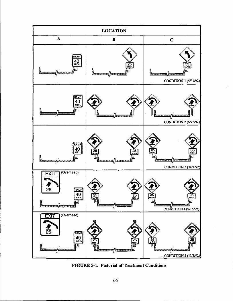
LOCATION
A B C
CONDITION 1 (5/31192)
CONDITION 2 (6125192)
CONDmON 3 (7121/92)
l~r·rhM~ 25
l I : ;. •• :;;. ••••••••••••••••••••••••• , ..................... J' ............ :
I~remea~ 25
FIGURE 5-1. Pictorial of Treatment Conditions
66

had to be greater than the threshold speed entered by the user. The program logic which activated the lights also turned them off after 5 seconds.
Modification of TC 1 Data
After collecting and evaluating the data representing the "no treatment" (TC 1) scenario at Location A, there was clear evidence of a problem with Location A data. Sufficient IRD raw data were available for Locations Band C. The problem was only with Location A. At the time of this discovery, researchers perceived at least three viable options for overcoming this deficiency instead of postponing subsequent test phases. At that time, the project sponsor desired to maintain the established schedule of monitoring each phase approximately one month.
The first option would have utilized a large sample of raw data collected by using non-IRD classifiers a few months prior to the beginning of the current phase of research. One of these systems was the CTR system and the other used a PAT classifier and the same permanent inductive loop/piezo system as used for this study. Of these two, the PAT system data were the most promising. Unfortunately, the researchers who deployed and monitored that system had not verified its accuracy, and this lack of calibration subsequently rendered the data unacceptable. To compound the problem, too much time had lapsed between PAT data collection and the time period of the missing data.
The second option was to wait until all warning devices had been tested and either remove or cover the newly installed traffic warning devices so as to replicate the before condition. However, after thoroughly evaluating this option and considering that these signs had been in place for over a year, it was decided that this covering or removal would not necessarily represent an equitable comparison of the before condition. This was due, in part, to a substantial number of trucks categorized as repeat traffic. It was postulated that a "learning effect" occurred in repeat drivers such that their driving behavior, after being repeatedly exposed to the signs, was based on their memory of the signs and/or on past knowledge of the ramp's geometrics. Thus, removal of the signs would not necessarily cause them to revert to their "before" behavior.
The third option would utilize the generous IRD bin data sample to estimate the truck speed distribution at Location A based on a limited raw data distribution. This process will be described in more detail later. The reason the bin data could not be used without this transformation was that speed bins aggregated all vehicle types, and the analysis needed to isolate truck speeds. By a process of elimination, this method offered the greatest promise for accurately replicating the missing data.
The lack of Location A Treatment Condition 1 raw data did not compromise the remainder of the study, but the missing raw data eliminated the potential for matching vehicle speeds as with other analyses. The comparison for TC 1 would still only allow comparison of group data and not paired data.
Conversion of the bin data representing TC 1 began with identifying a time period of raw data that would represent both the desired time periods and the desired locations on the ramp. The greatest need for data existed for TC 1 at Location A, although the same process was extended to include other bin data at Band C in order to compare with existing raw data to verify the accuracy
67

of the conversion process. Raw data from June 25, 1992, and June 30, 1992, at Location A served as the distribution to apply to the bin data representing the "before treatment" condition.
To reiterate, the reason for having to convert the bin data was that speed bins contained an aggregate of all vehicle classes, and truck speeds had to be separated from speeds of other vehicles. This process effectively created a distribution of truck speeds by segregating raw data into exactly the same speed bins as those used for the bin data set. See Appendix A for IRD speed bins. The next step removed bin numbers 1, 13, and 14 from further consideration, thereby eliminating speeds under 32 kmlh (20 mi/h) and over 129 kmlh (80 milh). The percentage of trucks within each of the remaining 11 speed bins, as calculated from the selected raw data files, formed the basis of the converted data set. For example, if the selected raw data file had 100 trucks and 900 other vehicle types within the speed range of 66 to 80 kmlh (41 to 50 milh), then 10 percent of the total (aggregate) vehicles in the 66 to 80 kmlh (41 to 50 milh) bin data would be trucks in the converted distribution. The process continued likewise for each speed bin, establishing a percentage of trucks for each one, and creating a new distribution of trucks only.
STATISTICAL TESTS ON TRUCK SPEED DATA
The Analysis of Variance
This statistical analysis depends primarily on the analysis o/variance (ANOVA), because of its robustness in inferring differences in population means when two or more samples are involved. Another statistic will also be used in this chapter to supplement the ANOV A; it is the Duncan multiple range test. The purpose for including the Duncan test is to provide information on the individual (speed) sample means which would not be available from SAS ANOVA output. The Duncan test also yields pairwise comparisons of sample means, determining where statistical differences exist between mean values (47). However, this function was not used in these analyses except in a secondary role because of ANOVA's superiority over multiple range tests for comparing multiple sample means.
One of the basic assumptions in using ANOVAis that the speed data fit the Standard Normal Distribution. When plotted, large samples of speed data for the various treatment conditions fit a symmetrical "bell-shaped" curve that is centered on its mean value, implying a normal population. Other assumptions underlying the ANOV A are random sampling methods, a common variance, and equal population means. SAS offers two procedures (pROGs in SAS terminology) which are appropriate for conducting the analysis of variance by computer. These, in SAS parlance, are the PROC ANOVA and the PROC GLM (General Linear Model). This research consistently utilizes the PROC GLM because it is the appropriate procedure where sample sizes differ among samples.
The Null Hypothesis
The fundamental purpose of the analysis of variance in this research, using the GLM procedure, was to identify statistically different sample means and to draw inferences about their respective population means. The assumption of equal population means coincides with the basic null hypothesis for this research, using the test parameter of speed reduction between monitoring stations.
68

The null hypothesis states that all speed reduction population means are equal for all treatment conditions. Equation (5) is a mathematical representation of the null hypothesis.
(5)
where: Iln = Population mean for Treatment Condition "n"
The alternate hypothesis, HA> is that at least one of the population means differs from the others. The probability of a Type I error, a, in all tests will be 0.05. The test statistic used by the ANOVA procedure to test equality of means is the F test using the ratio of the between sample variance and the within sample variance (48). This relationship is expressed mathematically as shown by Equation (6).
where: SB 2 = sample variance between speed samples sw2 = sample variance within speed samples
(6)
Sample variance is often thought of as the sum of squares divided by its degrees of freedom. Depending on its context, a sum of squares divided by its degrees of freedom is also referred to as a mean square. Thus, ~ 2 can be called the mean square between samples and Sw 2 can be called the mean square within samples. This is consistent with the usual terminology used in an ANOV A table, and it is consistent with SAS output produced by this research.
The null hypothesis of equality of t speed population means is rejected if the calculated F exceeds tabulated F values for a=0.05, dfB = t - 1, and dfw = n - t. In this fundamental null hypothesis, the number of population means, t, is 5 and sample size, n, is 2,401. In subsequent tests, the number of means and the sample sizes sometimes vary. Rather than relying on a predetermined a value (as 0.05 in this study), SAS generates the actual value corresponding to the significance level. SAS output calls this variable "PR>F," and some statistics texts call this value ''p'' (48). Either variable name represents the actual probability of a Type I error, and it provides more information to the user than a simple accept/reject scenario. In the various SAS outputs discussed below, if the computed PR>F value is less than a = 0.05, then the treatment will be declared significant. In some cases, the treatment will be declared highly significant if the PR>F value is substantially less than 0.05, say 0.0001.
In the paragraphs to follow, results will reflect several tests of significance that were required to completely understand the effects of the warning devices. This process starts with the preestablished data analysis plan, comparing speed reductions between A, B, and C based on treatment conditions. However, it was intuitively obvious that initial speed (at A or B) should be included in this first model. Thus, the model to test the null hypothesis stated above compared speed
69

reductions for each treatment condition in the presence of, or after accounting for, initial speed at either A or B. There were subsequent tests using ANOVA that became necessary as a result of the original data analysis plan or as SAS output indicated. For example, the original analysis plan included an investigation of weight as a possible explanation of speed reduction. However, it could not have anticipated all of the interaction terms in SAS output requiring additional SAS runs to understand the reason for significance. The text to follow describes the results of each ANOV A and their implications.
EFFECTIVENESS OF TREATMENTS BASED ON SPEEDS
Selection of Test Criteria
The independent variables that were deemed important include the general treatment conditions, but other statistical tests were also necessary. These tests evaluated the impacts of several factors in explaining the variability in speed data. Included were: the initial speeds (either at A or B), the effect of the active system "lights on" versus "lights off," peak period versus off-peak, day versus night versus dusk, vehicle weight, considerations of only combinations and only noncombinations, and the novelty effect of newly installed signs.
Speed differences of importance to this study required the creation of data sets using the following combinations of sites: AB, AC, BC, and ABC. Comparisons used speed change (as opposed to spot speeds) between these locations as the dependent variable to determine the effects of treatments, although the initial spot speeds at either A or B were important independent variables. For speed changes between AC and BC, comparisons usually used initial speeds at location A, although a few BC comparisons used initial speeds at location B. Appendix E contains the useful SAS outputs.
General Statistical Results
Table 5-1 summarizes speed sample means and standard deviations for all five treatment conditions utilizing all of the available data for each treatment condition. TC 1 uses bin data, whereas all others use raw data. Raw data are preferable to bin data due to the conversion process required for TC 1 bin data and the matching of same-vehicle speeds which is available only from raw data.
The remainder of the data analyses will omit TC 1 because evaluations of speed reductions require matching. Table 5-2 utilizes matched speed data to form a comparison of general speed reductions (in milh) among the various systems. It should be noted that TC 5 results in this table include both trucks which caused the lights to flash and those that did not cause them to flash. Therefore, it does not provide a pure comparison of only truck speed change when the lights were activated versus those when it was not activated. That comparison will be provided in a later section of this document. The total sample size for Tables 5-1 and 5-2 was 2,401 trucks of classes 5 through 13.
70

Table 5-1. Summary of Speed Parameters by Condition
TC 1 TC2 TC3 TC4 TC5 Parameter Bin Data Raw Data Raw Data Raw Data Raw Data
LOCATION A
n 7,695 167 109 667 1452
Mean 85.8 86.1 85.3 84.5 83.5
Std. Dev. 9.53 9.11 7.76 8.77 8.97
LOCATIONB
n 3205 167 109 667 1452
Mean 77 77 76 76 74
Std. Dev. 8.81 9.76 8.45 8.68 9.03
LOCATIONC
n 6130 167 109 667 1452
Mean 67.8 66.7 66.7 65.7 63.6
Std. Dev. 7.91 9.16 7.74 8.13 8.24
Note: Speeds and Standard Deviations are in units ofkmlh.
Table 5-2. Mean Speed Reduction Among Treatment Conditions
I Ramp
I I I I I Section TC2 TC3 TC4 TC5
AB 8.77 9.11 8.74 9.39
BC 10.79 9.55 10.03 10.59
AC 19.56 18.66 18.77 19.98
Note: Speed reductions are in units ofkmlh.
71

Specific Statistical Results
Beyond the basic considerations of spot speed and speed reduction are many of the details essential to understanding the effectiveness of each treatment condition. Table 5-3 shows the outcome of SAS runs using the main effects of Treatment (variable "Treat") and Speed (variable "SpeedA" or "SpeedB"). In this tabulation, the speed differences were for trucks as they traveled from points A to B, B to C, and A to C. In general, treatment was significant (at D=0.05) as represented by tabulated values ofPR>F less than 0.05. The exception was the speed change from B to C using initial speeds at A, labeled BC(A). Thus, these results indicate that the null hypothesis of no treatment effect in the presence of initial speed is rejected in all but one of the four models. In this table and others, initial speed was almost always highly significant. One would expect faster trucks to decelerate more than those traveling slower, all other factors being equal. One additional result shown by this table was that all Treat*Speed Interactions were non-significant.
The PR>F values presented in tabulated summaries come from the SAS Type III Sum of Squares. The reason Type III was used instead of Type I was that the Type I considers each variable in the sequence in which it was input, without consideration of what other factors are in the model. The Type III, on the other hand, considers each variable "in the presence of' other independent variables in the model. Type I and Type III Sum of Squares are equal if the model has only one main effects variable.
The table also shows output values of the variable SPD _ DIF, which was created for SAS runs to represent the difference in speeds (in milh) between defined points on the ramp. The ordering of sample means on the right-hand side of the table came from the Duncan multiple range test. These results show that, in the models tested, TC 5 and TC 2 were usually the most effective treatments, although these two TC's were not always statistically different from each other or from TC 3 and TC 4. Specifically, in data sets BC(A) and BC(B), the Duncan results showed that the sample means for TC's 2, 5, and 4 were not statistically different from each other and that means for TC's 5, 4, and 3 were not statistically different from each other.
Initial Speeds. Table 5-3, using SpeedA and SpeedB as variables, shows that initial speeds were always highly significant in explaining the speed reductions of trucks. SAS results were expected to verify that trucks traveling faster at Location A generally decelerated more than slower vehicles by the time they reached Locations B and C. Testing this hypothesis utilized three speed bins to determine the effects of initial speeds in explaining the differences in speeds at downstream locations. The bins were selected based on resulting sample sizes and logical break points. Speed ranges used for bins were: 32 to 79 kmlh (20 to 49 mi/h), 80 to 95 kmlh (50 to 59 mi/h), and 97 to 129 kmlh (60 to 80 milh). Table 5-4 summarizes the speed reductions based on initial speeds at A orB.
The Active System. In order to directly test effects of the lights beginning to flash as a truck approached, the vehicles recorded in CTR output files had to be matched with vehicles from IRD output files. A SAS program was written to expedite this process, but sample sizes were so small that the matching was redone manually. This resulted in a modest increase in the sample size. Clock times and vehicle lengths on both the CTR and IRD systems constituted the matching criteria. Matching vehicles between the two systems based simply on truck speeds would not have been
72
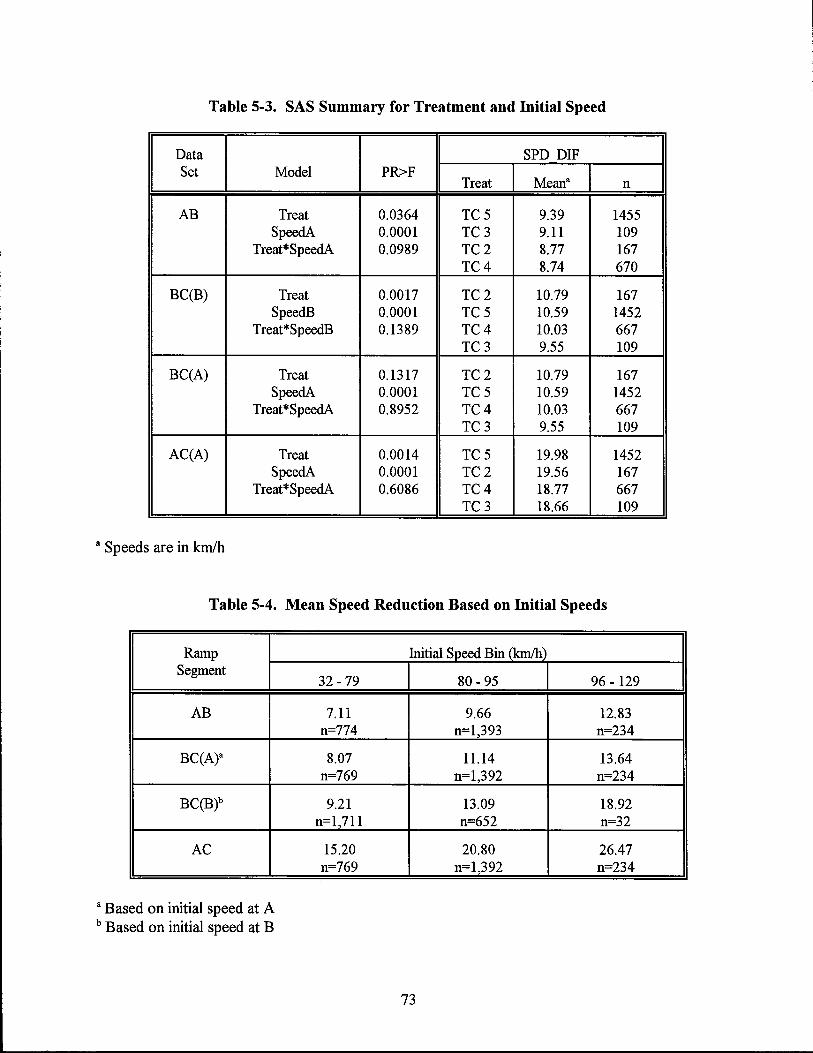
Table 5-3. SAS Summary for Treatment and Initial Speed
Data SPD DIF Set Model PR>F
Treat Meana n
AB Treat 0.0364 TC5 9.39 1455 SpeedA 0.0001 TC3 9.11 109
Treat*SpeedA 0.0989 TC2 8.77 167 TC4 8.74 670
BCCB) Treat 0.0017 TC2 10.79 167 SpeedB 0.0001 TC5 10.59 1452
Treat*SpeedB 0.1389 TC4 10.03 667 TC3 9.55 109
BCCA) Treat 0.1317 TC2 10.79 167 SpeedA 0.0001 TC5 10.59 1452
Treat*SpeedA 0.8952 TC4 10.03 667 TC3 9.55 109
ACCA) Treat 0.0014 TC5 19.98 1452 SpeedA 0.0001 TC2 19.56 167
Treat*SpeedA 0.6086 TC4 18.77 667 TC3 18.66 109
a Speeds are in kmlh
Table 5-4. Mean Speed Reduction Based on Initial Speeds
Ramp Segment
AB
BCCA)a
BCCB)b
AC
a Based on initial speed at A b Based on initial speed at B
32 -79
7.11 n=774
8.07 n=769
9.21 n=1,711
15.20 n=769
Initial Speed Bin (km/h)
80 - 95 96 -129
9.66 12.83 n=1,393 n=234
11.14 13.64 n=1,392 n=234
13.09 18.92 n=652 n=32
20.80 26.47 n=1,392 n=234
73

accurate enough because speeds varied slightly between CTR and IRD outputs and because not all trucks that exceeded the preset speeds initiated the lights.
Gathering data for the "lights off" condition required monitoring truck speeds during time periods when the CTR system was turned off or was not functional (e.g. due to power outages). These data provided the best comparison to "Lights On" without introducing significant bias to the analysis. The alternative of comparing lights on and lights off while the CTR system was fully functional would, in all likelihood, have biased the results because of the differences in vehicles between the two data sets.
Table 5-5 summarizes SAS output related specifically to effectiveness of the active system in reducing truck speeds. These results include two levels of the active system, on and off, and two initial speed levels, 80 kmlh to 95 kmlh (50 milh to 59 mi/h) and 97 kmlh to 129 kmlh (60 to 80 mi/h). Initial speeds were highly significant in the first model, but the active system was not significant in the presence of initial speed nor was the interaction term significant. Subsequent SAS runs omitted initial speeds and evaluated AB speeds by separating the two speed categories. CTR was not significant in either the high or low speed categories for the AB data set. However, a similar analysis using the AC and BC data sets omitting speed as a factor showed that CTR was significant. This clearly indicates that speed reductions were significantly greater between Band C with the active system in place than without the active system. It also suggests that truck drivers did not react quickly enough to the lights for their deceleration to be significantly different from the no lights condition between A and B.
Table 5-5. SAS Outcome for Active Device
Data SPD DIF Set Model PR>F
Treat MeanR n
CTR2AB2 CTR 0.6783 off 10.26 84 Speed 0.0002 on 10.05 70
CTR*Speed 0.8009
CTR2ABSH CTR 0.9355 off 14.96 7 on 14.72 14
CTR2ABSL CTR 0.3434 off 9.82 77 on 8.89 56
CTR2AC CTR 0.0006 off 18.93 140 on 22.25 57
CTR2BC CTR 0.0193 off 10.90 65 on 13.19 57
a Mean Speed in km/h.
74

Peak/Off-Peak. The weekday peak period on this ramp occurred in the afternoon from 4:00 p.m. to 7:00 p.m. Observations indicated that traffic speeds did not typically decrease substantially during this period, although traffic volumes were somewhat higher than they were during off-peak time periods. Of several SAS runs including peak period, none found any main effects or interactions to be significant. SAS runs used Treatment, SpeedA or SpeedB, Peak, and interactions in each model.
DaylNight/Dusk. Comparison of day versus night truck speeds began with establishing times for dawn and dusk throughout the data collection period. Then, the process defmed daytime as one hour after sunrise to one hour before sunset and nighttime as one hour after sunset to one hour before sunrise. Dusk was the remainder. Data sets used to test the day/night/dusk effects were AB, AC, BC using initial speed at B, and BC using initial speed at A. Findings showed that truck speeds were highest during the daytime, followed by night speeds, and the slowest speeds were during dusk. There was no statistical difference in the amount these vehicles decelerated during these periods, however. In other words, neither main effects nor interaction effects of these conditions were found to be significant in any tests.
Vehicle Weight. Loaded trucks typically have higher centers-of-gravity (c.g.) than unloaded trucks, resulting in lower roll stability as compared to unloaded trucks. The null hypothesis for this evaluation was that there was no difference in truck speeds due to loading. The final phase of data collection on this project included collecting weight data using a weigh-inmotion system upstream of the ramp. The WIM system collected data only on combination trucks in the right lane. An observer at the site recorded the following visual information on each vehicle weighed by the WIM system: vehicle number, time (hour, minute, and second), body type, whether loaded (if apparent), and distinctive characteristics.
This evaluation compared speeds of loaded trucks with those of unloaded trucks, and loaded trucks were further subdivided into c.g. height categories. Unfortunately, defmitive c.g. information was not available; only the weight and trailer type were used to infer the c.g. height in most cases. For purposes of this study, loaded vans and loaded tankers were considered to have high c.g. 's whereas others, such as flatbeds, required visual determination. In some cases of flatbed or lowboy trailers, the c.g. height could be categorized by observation, although their reliability was subject to question. For this analysis, researchers defmed loaded trucks as vehicles with gross vehicle weights (GVW) of 18,160 kg (40,000 lb) or greater.
Due to problems in the data that did not surface until after data collection was complete, the sample size was significantly smaller than needed for the analyses intended. Perhaps because of the resulting small sample size, the statistical test did not fmd that weight was a significant factor in explaining reductions in truck speeds.
Table 5-6 provides a summary of the SAS weight results. Two models show weight being significant, but these results must be interpreted carefully. Results from the WGTAB data set indicate that weight in the presence of initial speed is significant; however, speed is not. This causes immediate concern because speed in all other models was significant. The Speed*Weight interaction was also significant, suggesting the need for further evaluation. In the WGT ABSL
75

Table 5-6. SAS Outcome for Vehicle Weights
Data SPD DIF Set Model PR>F
Treat MeanR n
WGTAB Speed 0.2582 unload 10.98 17 Weight 0.0072 load 8.66 56
Speed*Weight 0.0067
WGTABSH Weight 0.9724 unload 10.09 15 load 10.14 30
WGTABSL Weight 0.0051 unload 17.71 2 load 6.94 26
WGT2AB Type 0.3629 van 10.00 38 flat 8.69 20 unk: 7.82 14
WGT3AB CentGrav 0.2358 high 10.06 44 low 7.92 13 unk: 7.82 14
a Speed in km/h
data set, which used only the slow initial speed bin, weight was also significant. However, the extremely small sample (n=2) of unloaded trucks could be a factor. Neither the type nor the c.g. height were significant in explaining speed variations; although the ranking by the Duncan multiple range test was reasonably consistent with anticipated results. Both the van in the "Type" model and the high c.g. in the "CentGrav" model exhibited the highest speed reductions among the categories tested.
CombinationINon-Combination Trucks. Drivers of combination trucks could possibly behave differently than non-combination drivers in negotiating this connector. Therefore, the following analysis investigated speed data by separating combination trucks and non-combination trucks into separate classes. For the combination only group, treatment was significant in the presence of initial speed in AB and AC data sets but not in BC(A) or BC(B). Treatment Conditions 2 and 5 consistently exhibited the highest speed reduction among the four TC I S for combination vehicles alone.
In the non-combination truck group, treatment was significant in the presence of initial speed in the AB, BC(A), and BC(B) data sets. The Treat*Speed interaction term was significant in the AB data set, so subsequent SAS runs separated speeds into three categories of high, medium, and low. The high speed was the only one of the three that was significant.
76

The Novelty Effect. A learning effect of the devices tested in this study by repeat drivers may have existed. In other words, a truck driver's ftrst encounter with a new device might cause a greater reaction than when he/she sees it at a later time. The "novelty effect" tends to wear off after repeated encounters, and its effects may stabilize at some lower response level than the ftrst time(s). There were undoubtedly repeat truck drivers using this ramp on a daily basis according to observations. Construction vehicles (e.g. aggregate trucks hauling materials to the US-59 construction project) and solid waste haulers were common users of the ramp who might have seen the various treatments on a daily basis. These drivers would probably not react the same as drivers who were totally unfamiliar with the ramp and who encountered the warning devices for the ftrst time. Insufficient data existed to statistically evaluate this phenomenon.
Speed Reductions of the Fastest Trucks
The measure of success of any traffic warning system depends in large measure on how well the results fulfilled the objectives. Speed reduction was a generally established objective from the outset of this research, however, the critical speeds were recognized as those that could lead to loss of control type accidents. Accident reduction was the ultimate objective, but measuring results by monitoring accidents would have required much more time and other resources than monitoring speeds. The foregoing analyses tested mean speeds; but reductions in mean speeds do not necessarily reflect a reduction in speeds of the fastest trucks.
Figures 5-2, 5-3, and 5-4 provide a comparison of truck speeds at Locations A, B, and C, respectively. Before considering these results, one must realize that these graphics are not intended to convey statistical significance. The sources of these results were raw data for TC' s 2 through 5 and bin data for TC 1. At Location A, speeds of the fastest trucks (85th and 95th percentiles) exhibited a generally declining trend. The only treatment expected to significantly impact speeds at A would have been TC 4, which included the overhead sign placed upstream of A. There are at least three possible explanations for the decline in the slowest trucks from TC 3 through 5. These include: the learning effect that could have occurred by repeat drivers, effects of the overhead sign near the gore; and random variation. Because of their slow speeds, only a few of these truck drivers would have been confronted with the flashing lights. TC 5 was in place long enough to span minor fluctuations, negating the short-term effect of random variations.
At Locations Band C, these same two (85th and 95th) percentile groups exhibited decreases of similar magnitudes as at Location A. Again, the slowest trucks decreased their speeds from TC 3 through TC 5.
COMMENTARY ON TRUCK SPEEDS
The Texas Department of Transportation had installed advisory speed plates on the ftrst and second curves on this connector of 40 km/h (25 milh) and 56 km/h (35 mi/h), respectively. Speed data show that trucks travel signiftcantly faster than these warning speeds, especially on the first curve. This thought process evolves into two questions: what is the actual maximum safe speed for various vehicles, and why is there such a discrepancy between observed speeds and the advisory speeds.
77

-.!: - 90 E ~ - 85 'U Q) Q) 80 a. w
75
70
65 TC 1 TC2 TC3 TC4
Treatment Condition TC5
95th 85th
50th 25th
10th
Figure 5-2. Cumulative Speed Distribution Values for Location A
95
90
85
I 80 'U Q) 75 Q) a.
W 70
~_f$i. 92 92
65
60+-----+-----1------r----~----~ TC3 TC4 TC5 TC 1 TC2
Treatment Condition
95th 85th
50th 25th
10th
Figure 5-3. Cumulative Speed Distribution Values for Location B
78

85
80
_ 75
~ ~ 70 .....,
-g 65 Q) Co
en 60
82
~~ 55
50+------r----~------+_----_r----~ TC 1 TC2 TC3 TC4 TC5
Treatment Condition
95th 85th
50th 25th
10th
Figure 5-4. Cumulative Speed Distribution Values for Location C
A Mathematically-Derived Maximum Speed
Using the mathematical relationships discussed in Chapter 3 and some assumptions regarding design vehicle parameters, one can derive maximum speeds for trucks on the two horizontal curves on this connector. Design plans indicate that the sharpest curve segments are 12-degree curves; on-site measurements show that the maximum superelevation rate for both curves is 0.08 mlm (0.08 ftlft).
The Federal Highway Administration sponsored a study (3.3.) which concluded that the point mass representation is appropriate for use in detennining the net side friction demand of both passenger cars and trucks, but certain caveats apply. One is that significant differences exist in friction demands among the various tires of a large truck as compared to the approximately equal sharing of friction demands among the four tires of a passenger car. The net result of this variation in trucks is approximately 10 percent higher side friction in trucks than passenger cars. Another consideration not inherent in the Green Book's presentation of the point mass model is a lack of consideration of driver input as the vehicle negotiates the curve. In reality, drivers oversteer along the curve, increasing the side friction above that calculated by using the nominal curve radius. Finally, truck tires use a harder rubber that reduces their tractive capabilities. Equation (3) in Chapter 3, reproduced below as Equation (7), is the same as that provided in the
79

Green Book (1). The noted caveats will be used in the following analysis to follow to modify Equation (7) so it better reflects reality for trucks.
v2
/= -- - e 127R
Rearranging terms and solving for V, the speed in km/h, Equation (8) results.
v = J127 R (e + f)
Known values: e = 0.08 m/m (0.08 ft/ft) R = 1747/D = 1,727112 =145 m (477 feet)
(7)
(8)
From Green Book Table ill-6, the computed radius corresponds closely with a design speed of 64 km/h (40 milh ), using the measured maximum "e" of 0.08 m/m (0.08 ft/ft) and an assumed maximum "f' of 0.15. This assumed speed also corresponds to the RAMP 40 MPH sign used on the ramp.
In the discussion of failure modes, both skid and roll must be included. For combination vehicles, skid often results in jackknife, which subsequently sometimes results in rollover. In order to determine the maximum f that is applicable to impending skid, the assumptions listed below and cited in Harwood and Mason (41) must be considered.
• The peak friction coefficient applicable to cornering at the appropriate design speed is 1.45 times the locked wheel braking value for wet pavement in the Green Book Table ill-I. For the apparent 64 km/h (40 mi/h) design speed, the nominal "f" value is 0.32.
• The tire pavement friction generated by truck tires is only 70 percent of that of passenger car tires.
• The analysis should allow a 15 percent steering fluctuation as suggested by Ervin et al. (35). This results in an effective radius, ~ff = 123 m (405 ft).
• Due to wider variations in friction demand in truck tires, "effective side friction demand" is approximately 10 percent higher for trucks than for cars. Thus, the friction demand for trucks is slightly higher than Equation (7) results.
In the use of Equation (8) to calculate the maximum "safe" speed where skid is imminent, and if the radius is reduced by 15 percent and the superelevation is established, then the only remaining factor requiring modification is the coefficient of friction. The three previously noted corrections are shown below in the following order: correction from locked wheel braking to cornering, correction for reduction in pavement friction from car to truck tires, and correction due to "effective side friction demand" higher in trucks.
80
(0.32)(1.45) • 0.46
(0.46)(0.70) = 0.32
(0.32)(1.10) = 0.36
Thus, the speed which could precipitate skid under the foregoing assumptions is:
v SKID: J(127 )(123 )[0.08+0.36] = 83kmlh (SImi/h)
The second analysis determines the critical speed for rollover, again through consideration of the vehicle as a point mass. One of the conclusions of Chapter ill was that an appropriate rollover threshold value for use in design, although admittedly conservative, is 0.30g. The side friction demand expressed by Equation (7) above is mathematically equivalent to the unbalanced lateral acceleration (~eJ expressed by Equation (3) in Chapter 3. The unbalanced lateral acceleration represents the resultant forces acting on the vehicle that tend to make it skid or overturn. Therefore, solving Equation (8) again with the rollover threshold of 0.30g is as shown.
VROU= J(127 )(123 )[0.08+0.30] = 77kmlh (48milh)
In many cases, the actual sustainable maximum speed for combination vehicles passing through the two horizontal curves on this connector would be faster than these calculated values. V SKID was based on wet pavement and V ROLL was based on a conservative value of rollover threshold. However, there are destabilizing factors not included in these two results that are not easily quantified. Included are hydroplaning (often resulting in jackknifmg) and load shift.
Advisory Speed versus Safe Speed
Advisory speeds are set today according to criteria established over 50 years ago. In 1937, the Missouri State Highway Department began experimenting with a ball bank indicator to measure the centrifugal forces acting on a vehicle. The Bureau of Public Roads also tested this device at approximately the same time period (46). The ball bank indicator is a simple device consisting of a curved glass tube of a standard radius, filled with a liquid in which a steel ball is free to move. The operative forces acting on the ball are gravity and the lateral acceleration as the vehicle traverses a curve, and there is a damping effect created by the liquid. Gravity pulls the ball toward the center (low point) of the curved cylinder, whereas centrifugal force pulls the ball toward the outside of the vehicle's curved trajectory. In the procedure used to establish safe speeds, an observer inside a test vehicle monitors the ball's movement relative to graduations (in degrees) along the outside of the cylinder. Early testing of the ball bank indicator showed that a
81

10-degree reading corresponded to a side friction factor of approximately 0.14 to 0.15, depending on the body roll of the vehicle (46). The ball bank reading in degrees is the sum of the centrifugal force plus the body roll angle minus the superelevation.
The AASHTO Green Book (1) recommends that design values of maximum allowable side friction be based on driver comfort. This has been described as the point at which drivers feel sufficient centrifugal force to discourage them from driving faster. The Green Book also allows reductions in side friction factors in mban areas due to higher driver tolerance. Not all states use exactly the same methods to establish comfortable side friction levels, although the resulting side friction factors appear to be reasonably similar. The range of ball bank readings, from 14 degrees for low speeds to 10 degrees for high speeds, seems to be generally accepted. According to Merritt (49), the spread in tolerable discomfort generally coincides with that found in the Traffic Control Devices Handbook and the Institute of Transportation Engineers Transportation and Traffic Engineering Handbook.
In general, the upper limit of the possible range of side friction factors represents a nearskid (or roll) condition. Obviously, highways are designed to avoid loss of control with an appropriate margin of safety, so the appropriate f value must be selected to avoid loss of control in both dry and wet conditions. Variables that can influence the value off include pavement texture, weather conditions, and tire condition. Generally accepted values of maximum side friction for new tires on wet concrete pavement range from approximately 0.5 at 32 km/h (20 milh) to approximately 0.35 at 97 km/h (60 milh). For smooth tires under the same wet concrete conditions, the value is approximately 0.35 at 72 km/h (45 mi/h). Commonly accepted among the various studies is that friction values generally decrease with increasing speed (1).
According to information available from the literature, no distinction by vehicle type in setting speeds on curves appears evident. While there are deftnitive differences in stability characteristics between cars and trucks, the empirically derived side friction factors resulting from "driver comfort" establish reasonable safety margins for both classes of vehicles as long as they do not exceed the design speed. However, as pointed out by Harwood and Mason (41), on horizontal curves designed in accordance with Green Book Table ill -6 with design speeds of 64 km/h (40 milh) or less, the most unstable trucks (those with high c.g.) can roll over at speeds of 8 to 16 km/h (5 to 10 mi/h) over the design speed.
The 1990 Green Book still uses some of the earliest criteria, adding values for higher speeds as necessary. Table ill -6 from the Green Book includes values of side friction for design speeds ranging from 32 km/h (20 mi/h) to 113 km/h (70 mi/h). The maximum coefficient of friction proposed by the Green Book for a 64 km/h (40 milh) design speed is 0.15. In order to verify driver "comfort levels" based on speed data collected on this connector roadway, the author created a speed distribution downstream of Location B within the sharpest portion of the fIrst curve. The new location is called B'. Because no speed data were collected between Band C, a speed proftle had to be created based on site observations and speed data. Comparisons of the assumed speeds within the curve and maximum safe speeds calculated earlier provided a check on this procedure.
82

The procedure used to create this distribution for trucks at the fIrst curve required making an assumption about the vehicle-specifIc deceleration that occurred between Band B'. Because speeds of each truck were known from raw data at Locations B and C, the upper and lower boundaries of deceleration rates could be calculated. The lower boundary represented a constant deceleration from B to C, whereas the upper boundary varied from a maximum at B to almost zero at C. This maximum reflected the value considered in Chapter 4 of 0.16 g, or 1.6 m/sec2 (5.2 ftlsec
2). For each vehicle in the data set, a speed was calculated for B', which was located 91 m
(300 ft) downstream of Location B.
The speed distribution for passenger cars and light trucks (classifIcations 2 and 3) was created from group speeds at Band C because these vehicles were very diffIcult to match accurately either by computer or by manual methods. Therefore, the speed distribution from B was simply "shifted" by an amount proportional to the distance of B' from B, assuming a straight line (constant) deceleration between Band C.
Table 5-7 is a summary of percentiles of vehicular speeds at Location B' and the corresponding side friction factors based on the foregoing narrative (using R=145 m [477 ft]). Because of typically differing failure modes of trucks versus cars, the calculated f values that approach stability limits represent impending rollover in trucks and impending skid in passenger cars. For a design speed of 64 km/h (40 milh ) and "e" of 0.08 m/m (0.08 ft/ft), the assumed maximum side friction factor for design is 0.15. All of the 3,500 car drivers represented in this sample were apparently willing to accept a higher discomfort level than that corresponding to a side friction value of 0.15. These observed speeds might be lower if the pavement were wet, although light to moderate rainfall did not generally reduce speeds signifIcantly on this connector.
Table 5-7. Calculated Side Friction Factors at Location B'
I Percentile
I Trucks
I Cars
I Speeds S:Qeed {km/h} I f S:Qeed (km/h} I f
95th 82.1 0.28 93.4 0.39
90th 78.9 0.26 90.2 0.36
75th 74.1 0.22 85.3 0.31
50th 68.4 0.17 80.5 0.27
25th 62.8 0.13 74.1 0.22
10th 58.8 0.11 69.2 0.18
83

For the trucks represented by these tabulated values, 95th percentile speeds approach the stability limits of some loaded trucks, and this is before consideration of the 15 percent steering fluctuation as proposed above. According to Ervin et al. (35.), a few loaded trucks on the nation's highways today have rollover thresholds as low as 0.27. Figure 3-1 depicts three combination vehicles with rollover thresholds of 0.31 (corrected for simulation error of 0.03 g) or lower along with their corresponding payload c.g. heights. In this same referenced study, Ervin et al. proposed a rollover threshold for design purposes of 0.30 g. Equation (4) from Chapter 3 is reproduced below as Equation (9) to be used to calculate the maximum lateral acceleration using this design value. Omitting the safety margin for the time being, the calculated maximum Cly is 0.26 g. According to estimates of truck speeds at Location B', the 90th percentile trucks are in jeopardy if they happen to be the most unstable trucks with the worst roll stability limits.
RT - 8M Dymu: -
1.15
where: Cly max = Safe lateral acceleration RT = Rollover threshold SM = Safety margin
(9)
The posted advisory speed for the ftrst curve on the 1-610 connector was inappropriate because it was too low. This was ostensibly demonstrated by the discrepancy between the posted advisory speed and actual vehicular speeds shown in Table 5-7. The 10th percentile speeds for both trucks and cars were faster than the advisory speed of 40 km/h (25 mi/h) set for the ftrst cmve. As noted previously, it was not intuitively obvious why the posted speeds differed for the two curves, leading to the possibility of an error in establishing the advisory speed for the ftrst curve.
The setting of advisory speeds significantly lower than the actual safe speed for all but the most unstable vehicles has been practiced in this country for too long, and it should be reevaluated. Over the past 50 years since today's criteria for establishing advisory speeds were first implemented, trucks have gotten larger and heavier, and cars have gotten smaller with improved stability in cornering. Centers of gravity for cars have gotten lower to the pavement while those of trucks have shifted in the other direction with increased gross vehicle weight ratings and trends in "cube out" conditions. This dichotomy in inherent vehicle stability on curves leads to the need to at least rethink the process of setting safe speeds. One of the research ideas emanating from this thought process is the feasibility of two systems -- one for unstable (loaded) trucks and one for cars and unloaded trucks. The author's observations of all vehicle types at many locations as they negotiate curves demonstrates that advisory speeds are set much lower than necessary for almost all vehicles. They are conservative for automobiles, as well as for many trucks.
All drivers, and especially truck drivers, need accurate advance warning information pertaining to the roadway, especially in unfamiliar surroundings. In truck driver interviews,
84
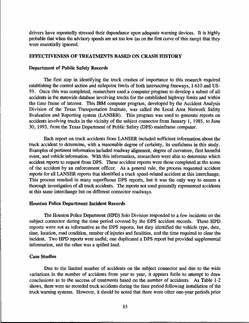
drivers have repeatedly stressed their dependance upon adequate warning devices. It is highly probable that when the advisory speeds are set too low (as on the first CUlVe of this ramp) that they were essentially ignored.
EFFECTIVENESS OF TREATMENTS BASED ON CRASH HISTORY
Department of Public Safety Records
The frrst step in identifying the truck crashes of importance to this research required establishing the control section and milepoint limits of both intersecting freeways, 1-610 and US-59. Once this was completed, researchers used a computer program to develop a subset of all accidents in the statewide database involving trucks for the established highway limits and within the time frame of interest. This mM computer program, developed by the Accident Analysis Division of the Texas Transportation Institute, was called the Local Area Network Safety Evaluation and Reporting system (LANSER). This program was used to generate reports on accidents involving trucks in the vicinity of the subject connector from January 1, 1985, to June 30, 1993, from the Texas Department of Public Safety (DPS) mainframe computer.
Each report on truck accidents from LANSER included sufficient information about the truck accident to determine, with a reasonable degree of certainty, its usefulness in this study. Examples of pertinent information included roadway alignment, degree of cUlVature, frrst harmful event, and vehicle infonnation. With this information, researchers were able to determine which accident reports to request from DPS. These accident reports were those completed at the scene of the accident by an enforcement officer. As a general rule, the process requested accident reports for all LANSER reports that identified a truck speed-related accident at this interchange. This process resulted in many superfluous DPS reports, but it was the only way to ensure a thorough investigation of all truck accidents. The reports not used generally represented accidents at this same interchange but on different connector roadways.
Houston Police Department Incident Records
The Houston Police Department (HPD) Solo Division responded to a few incidents on the subject connector during the time period covered by the DPS accident records. These HPD reports were not as infonnative as the DPS reports, but they identified the vehicle type, date, time, location, road condition, number of injuries and fatalities, and the time required to clear the incident. Two HPD reports were useful; one duplicated a DPS report but provided supplemental information, and the other was a spilled load.
Case Studies
Due to the limited number of accidents on the subject connector and due to the wide variations in the number of accidents from year to year, it appears futile to attempt to draw conclusions as to the success of treatments based on the number of accidents. As Table 1-2 shows, there were no recorded truck accidents during the time period following installation of the truck warning systems. However, it should be noted that there were other one-year periods prior
85

to treatment installation in which no truck accidents were recorded. So, rather than attempt an analysis based solely on the numbers of truck accidents, the more appropriate use of the available information is thought to be development of case studies. These case studies will provide information that could identify the factors responsible for the accident.
The case studies to follow provide detailed information on the truck accidents identified by this process and which could possibly be related to excessive speed. There were no truck accidents recorded in DPS records that were apparently attributable to high speeds during 1985, 1986, 1987, 1991, 1992, or 1993. Records show that the three remaining years, 1988, 1989, and 1990, produced nine accidents with yearly totals of two, one, and six, respectively.
Case Study Number 1. This case study is based on a report from the Houston Police Department providing information on an incident that occurred at 3:45 p.m. on February 11, 1988. The only vehicle apparently involved was a tractor-semitrailer, and the incident resulted in no injuries or property damage although one lane remained closed for two hours. The report did not provide a reason for the incident, but because it resulted in a spilled load it was assumed to involve excessive speed on a curve. The pavement was dry when the incident occurred. According to the report, the Solo Division arrived at 3:50 p.m., and the spill was removed by 6:00p.m.
Case Study Number 2. This case study and the remaining case studies are based on reports from the DPS, although HPD also provided a report on one other accident. This accident occurred at 6:30 p.m. on Thursday, March 17, 1988, on a wet surface; wind was also mentioned as a weather-related factor in the driver's comments. The vehicle was a 1985 Kenworth tractorsemitrailer registered in Texas. The investigating officer made the following comments: "No. 1 vehicle traveling eastbound Exit Ramp on 610 North Loop East to U.S. 59 northbound, flipped over on the left side due to load weight shifting, trailer hit the rail causing severe damage to the guardrail and road. " The driver provided the following comments: "1 exited onto the exit ramp at about 40 milk and when I came over the hill, the wind caught my load making it shift and flip my trailer over along with my rig." The report noted damage to the bridge rail and pavement as a result of this rollover. Both the driver and his passenger sustained non-incapacitating injuries. The enforcement officer's sketch of the site and the driver's comments suggests that the location was within or near the first curve. Contributing factors were "failure to control speed" and "failure to maintain load."
Case Study Number 3. This accident occurred at 1:30 p.m. on Saturday, October 22, 1988. The weather was clear and the pavement was dry. The vehicle was a 1978 Kenworth tractor-semitrailer registered in Texas. The semitrailer was a flat bed loaded with a large concrete block. The officer's comments were as follows: "Unit # 1 towing unit # 2 lost load while on northbound entrance ramp to Eastex Freeway. Load struck and damaged guardrail." The driver provided the following comments: "1 was going around the comer when the load came off the trailer." In his report, the officer estimated the bridge rail damage to be $16,700. The sketch provided with the report depicted the vehicle in the right lane in the first curve when the block fell off the trailer. A contributing factor was "speeding, under limit," and a citation was issued for "failure to secure load."
86

Case Study Number 4. This accident occurred at 3:30 p.m. on Tuesday, June 20, 1989. The weather was cloudy and the pavement surface was dry. The vehicle was a 1986 International tractor-semitrailer with Alabama registration. The semitrailer was a flatbed loaded with bulk solids. The officer provided the following description of what happened: "Vehicle #1 load shifted causing it to tum over on its right side colliding with vehicle #2 left side. Both were nonhbound . . Vehicle #1 then collided with the pavement." The driver of vehicle number one provided the following comments: "[ was watching two trucks on my right side and was looking at my rearview mirror and [ seen my wheels come up. [staned to slow but it was too late. [was doing around 40 to 50 milh. " Witness number 1 commented as follows: "We were behind him and doing about 25 to 30 milh. He was going a little faster than us. His cargo shifted; his wheels came up and he went over." A second witness provided these additional comments: "[ seen his load shifting and he came up on 2 wheels and went over. He was doing about 25 to 30 milh." The damage to the pavement was estimated on the report to be $300. The officer's sketch of the accident depicted vehicle 1 in the left lane and vehicle 2 in the right lane; the two trucks were side by side when vehicle 1 rolled over. The driver of vehicle 1 sustained a non-incapacitating injury.
Additional information was available from a report by the HPD Solo Division, which responded to this rollover. The HPD spent 5 112 hours at the site assisting with clean-up activities; their records show their arrival time being 4:00 p.m. and completion of clean-up at 9:30 p.m. According to the DPS report, there was no citation issued.
Case Study Number S. This accident occurred at 3:00 p.m. on Wednesday, May 9, 1990, on a clear day on dry pavement. The power unit of the tractor-semitrailer was a 1989 Peterbilt; the semitrailer was a flatbed loaded with "construction material." The vehicle was registered in Texas. The officer who investigated the accident provided the following comments: "Vehicle #1 nonh on U.S. 59 from [H-610, lost control of vehicle and rolled over, striking guardrail." The driver had these comments: "[ was nonh on 59 from 610 and my load shifted and [ rolled over." The accident report did not indicate any damage to the roadway. The officer's sketch on the report indicated that the vehicle was negotiating the first curve when it rolled over. The driver sustained a non-incapacitating injury during the accident. A contributing factor was "failure to control speed."
Case Study Number 6. This accident occurred at 1:40 a.m. on Wednesday, June 13, 1990, in clear weather on a dry pavement. The vehicle was a 1990 International tractorsemitrailer (body type not specified), registered in Iowa although the driver's home address was in Houston. The officer provided the following comments on the accident: "Unit #1 traveling nonh on the entrance ramp from Nonh Loop East to the Eastex rolled over when the weight in the trailer shifted to the right." The driver of the truck stated: "[ was going through the curve when the weight shifted in the trailer and caused me to roll over." One witness simply stated that .. . "the truck was not traveling fast." The accident report did not specify any damage to the roadway, although the officer's sketch showed scrape marks along the edge of the right-hand shoulder. The sketch also depicted the vehicle on the right-hand shoulder after it rolled over. The driver sustained non-incapacitating injuries during the accident.
87

Case Study Number 7. This accident occurred at 3:00 p.m. on Monday, July 30, 1990, on a clear day on a dry pavement. The vehicle was a tractor-semitrailer whose power unit was a 1984 Peterbilt tractor that was registered in Indiana, and it was towing a van semitrailer. The officer provided the following comments: "Unit #1 and #2 north bound on Eastex Freeway from entering ramp off 610 Loop, failed to drive in a single lane after losing control on curve rolled tractor trailer over on side." The driver had been taken to the hospital and did not provide comments. There was damage to the pavement due to the accident, although the extent of the damages was not specified. The officer's sketch depicted the vehicle just downstream of the second cmve where it rolled over on the left side of the ramp. The driver sustained incapacitating injuries during the accident. The officer who investigated the accident issued a citation for "failure to drive in a single lane." Other contributing factors were "took curve too fast" and "driver inattention. "
Case Study Number 8. This accident occurred at 12:34 p.m. on Thursday, November 22, 1990, in clear weather on a dry pavement. The vehicle was a tractor-semitrailer with a 1988 Kenworth power unit that was registered in Oklahoma, and it was towing a van semitrailer. The officer described the accident as follows: "Unit #1 eastbound North Loop East exit ramp to Eastex Freeway northbound. Unit #1 failed to maintain single lane and struckftxed object with right side of vehicle. Fixed object broke loose and fell to the North Loop East westbound and struck unit #2 and unit #3". The truck driver commented as follows: 'jot car cut me offwhen I swerved the tractor went on its side." The driver of vehicle number 2 (traveling on the freeway below the connector) provided these comments: "He was going too fast and flipped on his side. He knocked a street sign off the bridge, and itfell infront of me. " Driver number 3 (also on the freeway below) simply stated that he saw the same thing as driver number 2. The accident report indicated sign and bridge rail damage in the estimated amount of $5,000. The officer's sketch on the accident report depicted the tractor-semitrailer on its side within the first curve. Severity of the accident was limited to property damage; no injuries were reported. The driver received a citation for "failure to maintain a single lane."
Case Study Number 9. This accident occurred at 10:30 a.m. on Wednesday, November 28, 1990, in clear weather on a dry pavement. The vehicle was a tractor-semitrailer with a 1987 International tractor registered in Louisiana, and it was towing a flatbed semitrailer. The officer described the accident as follows: "Tractor and trailer taking exit ramp from North Loop East to Eastex. A 29,000 lb of roll steel came loose and struck the freeway exit ramp." The driver commented: "1 was taking the exit to Eastex Freeway from North Loop East when my load (29,000Ib) a roll of steel, came loose and dropped to the exit." The damage to the ramp was estimated to be $40,000. In the officer's sketch, the roll of steel came off the trailer within the first curve on the connector. There were no injuries reported, and the contributing factors listed by the officer were: "load not secured" and "speeding under limit."
Case Study Number 10. This accident occurred at 5:00 p.m. on Sunday, December 9, 1990, in clear weather on a dry pavement. The vehicle was a tractor-semitrailer with a 1983 Marmon power unit registered in Texas, and it was towing a flatbed semitrailer. The officer provided the following comments regarding the accident: "Vehicle #1 towing #2 was northbound on the Eastex Freeway entrance ramp. Vehicle #3 and 4 were southbound on the Eastex Freeway.
88

Vehicle #1 struck the retaining wall and rolled on its side. The load of pipe from vehicle #2 broke loose from said vehicle and fell below striking vehicle #3 and 4." The comment from driver number 3 was ''All we seen was stuff falling from the freeway." The damage to the connector roadway was estimated to be $3,000. The sketch provided by the officer did not show exactly where the truck impacted the barrier, although it was probably just downstream of the first curve but certainly upstream of the second curve. This general area could have resulted in the pipe falling on the southbound lanes of the Eastex Freeway as shown by the accident sketch. This accident resulted in incapacitating injuries to occupants of vehicle number 3. The officer issued a citation to the truck driver for "failure to maintain a single lane." A contributing factor noted by the officer for the truck driver was "driver inattention. "
Case Study Evidence
During the 8 112 year time period represented by the accident and incident reports, there were a total of 10 truck accidents or incidents that could possibly have been attributable to excessive speeds. Ofthese 10, Case Studies 1, 7, and 10 were not as clearly correctable by speed control countermeasures as the others. Crash information was inconclusive in number 1, and in numbers 7 and 10, driver inattention appeared to be the primary cause of the crash. There was also evidence that both trucks had safely negotiated at least one curve before crashing. One struck the bridge barrier and subsequently rolled over, and the other rolled over downstream of the second curve.
Of the remaining seven accidents, load shift and/or loss of load was reportedly a factor in all of them, while speed was noted explicitly by the investigating officer in four. All of them apparently occurred within the first curve on the ramp. In five of these remaining seven accidents, rollover resulted. The only case study that noted weather as a possible factor was Case Study 2 under driver comments, although its effect was discounted by the fact that the investigating officer omitted it in his contributing factors. The officer did include speed and failure to secure the load.
In summary, at least 7 of the 10 incidents or accidents appeared to result from excessive speed. These might have been prevented by appropriate warning devices in advance of the first curve. Maximum safe speeds calculated in this document are related to either skid or roll, and should not be construed to prevent load shift or load loss. Indeed, it is the responsibility of the owner and operator of the vehicle to ensure that the load is secured and does not create a hazard for other motorists.
89

~------------------------------------------------------------------------------------------------------------------------------------------------------------~

CHAPTER 6. SUMMARY INTRODUCTION
The purpose of this research was to investigate the effectiveness of traffic control devices in reducing the speeds of large trucks where potentially hazardous conditions exist on freeway to freeway connectors. The unique characteristics oflarge trucks require special attention by design and operations engineers in order to maintain the safest possible environment for all vehicles, especially where constraining geometric elements exist. Freeway to freeway connectors are examples of roadways where lower design speeds prevail, requiring speed reductions due to combinations of horizontal curves, vertical curves, and grades.
In perhaps the most definitive research conducted recently on freeway connectors, Leonard and Recker (30) used the Caltrans TASAS data base to scrutinize truck accident records over the 8 1/2 year time period from January 1, 1979 through July 31, 1987. They reported that among several causal factors related to loss-of-control, speeding was the most highly significant (p < 0.001). Speeding was a factor in 68.6 percent of allioss-of-control crashes, and it was a factor in 78 percent of the 17 connectors (of the total 200) with the highest number of truck crashes. A recent study by Hilton and Meyer (31) indicated that the worst type of crash with respect to injury was rollover, and its significance was compounded by its frequency. From 1979 to 1986, rollover occurred in almost 14 percent of all single vehicle truck crashes, and it resulted in over 60 percent of the total truck occupant injuries.
Because reconstruction of problematic freeway to freeway connectors is usually not feasible, other cost-effective countermeasures are used, at least in the short term. Recent research (1) revealed truck accident countermeasures used on freeway ramps, including warning signs, oversize barriers, continuously flashing lights, and increased superelevation. Some jurisdictions were using variations of the standard MUTCD (~) traffic control devices; others increased the size andlor number of devices or attempted innovative approaches at known problem locations. Although many of the innovative solutions were thought to have reduced the problem, none had been formally evaluated as to their effectiveness. Three other studies (.2., 10, 11) installed active warning devices to warn truck drivers, but only two actually tested their effects on truck speeds. Both of the study reports suggested positive elements of active truck signs, although only one showed reductions in truck speeds. It found that mean speeds at mid-ramp locations were lower with flashing lights than without. Furthermore, even though the flashing lights did not significantly increase compliance of trucks with posted advisory speed signs, they did significantly reduce the number of trucks traveling more than 8 km/h (5 mi/h) and 16 km/h (10 milh) faster than the calculated maximum safe speed. In the other study, the positive element was associated with correct truck driver recognition of the sign, leading the authors to suggest that it be considered at high accident locations.
STUDY PROCEDURE
This research tested a series of treatment conditions intended to serve as countermeasures to truck accidents by providing a warning to truck drivers. These roadway systems can be classified as passive devices and active devices. Active, in this case, means that the traffic warning system is dormant until preset conditions pertaining to vehicle height, speed, and length are met.
91

A significant portion of the initial phase of this study was devoted to identifying and testing appropriate methods of monitoring traffic on freeway connectors where the requirement for continuous and uninterrupted communications and electrical power along the connector created unique challenges. The selection and testing process for speed/classification systems resulted in the purchase of three stand-alone vehicle classifiers using their own power source (internal battery) while coordinating their internal clocks to avoid the necessity of communications. This time coordination provided the capability of "tracking" target vehicles, given the vehicle's speed at each monitoring location and the distance to the next monitoring location.
A roadside infrared (IR) beam system provided a redundant vehicle length classification system during the first four treatment conditions (TC's) of the research, but then its capabilities were enhanced to accommodate the TC 5 active device. The system was set to monitor vehicles that were over 4.88 m (16 ft) in length and over 2.16 m (7 ft 1 in) in height.' These dimensions reflect those of large trucks which are more likely to have high centers of gravity and thus be subject to rollover. A thorough evaluation of sensors used to monitor truck traffic throughout this study has been provided elsewhere (50).
The computerized statistics package used to evaluate the speed and weight data was the Statistical Analysis System (SAS) (16). The process of evaluating truck speeds on the ramp produced SAS programs designed to read matched truck speeds at Locations A, B, and C and determine speeds and speed reductions among the three locations.
EFFECTS OF WARNING TREATMENTS
Speed differences are the primary dependent variable upon which conclusions of treatment effectiveness are based. The results of all tests of significance are reported using the probability of a Type I error, D, equal 0.05. The null hypothesis tested by ANOVA was that there was no treatment effect for TC 2, 3, 4, and 5. Because initial speed was essential in explaining speed reduction of trucks, it was generally included in the test of treatments.
• The main effect of Treatment was significant in the presence of Speed for trucks traveling from points A to B, B to C, and A to C. These correspond to data sets AB, BC(B), and AC(A). However, Treatment was not significant from B to C using initial speeds at A. The null hypothesis of no treatment effect in the presence of initial speed is rejected in all but one of the four models.
• In the models tested, TC 5 and TC 2 were usually the most effective treatments (exhibited the highest speed reductions), although these two TC's were not always statistically different from each other or from TC 3 and TC 4.
• In the pure comparison of the active system, in which lights came on in one data set and did not in the other, speed reductions were significant in AC and BC data sets, but not in AB data sets, suggesting that truck driver response to the lights occurred downstream of Location B.
• Truck weights were not significant in any tenable test results. Separation of trucks into the categories of combination and non-combination trucks, peak/off-peak periods, and
92

day/night/dusk periods was not helpful in understanding variations in truck speeds.
• At Location A, the 85th and 95th percentile truck speeds exhibited a generally declining trend. The only treatment expected to significantly impact speeds at A would have been TC 4, which was the overhead sign placed upstream of A.
• At Locations Band C, the 85th and 95th percentile groups exhibited decreases of similar magnitudes as at Location A. Again, the slowest trucks decreased their speeds from TC 3 through TC 5.
SOME DESIGN IMPLICATIONS OF STUDY FINDINGS
Study findings have implications related to several design aspects of the driver-vehicleroadway environment. Some of these were available in the literature while others resulted from either the accident history or the speed study inherent in this research.
Driver Considerations
• Preferences of truck drivers interviewed in Maryland and Virginia included the following elements: a tipping truck silhouette, a diagrammatic curve arrow, an advisory speed, the legends ROLLOVER HAZARD or TRUCK CAUTION. Legibility testing strongly supported the use of symbolic signs but with a separate advisory speed plate underneath. Finally, truck drivers expressed the desirability of using both advance warning signs and flashing lights in combination with these at-ramp signs.
• Statements of Texas truck drivers regarding advisory speeds revealed that they believe speeds are set for automobiles, requiring trucks to travel even slower than posted speeds to be safe. However, these comments from both groups of Texas drivers were inconsistent with findings of actual speeds on the I-610/US 59 connector and with the author's observations of trucks elsewhere.
• Of the seven single-vehicle truck accidents that were recorded on the I-610/US-59 connector in an 8 112 year period, excessive speed was noted explicitly by the investigating officer in four. Rollover was a result in five of these seven accidents.
Vehicle Design Parameters
• Using the point mass model, a wet pavement coefficient of friction, and assumptions based on characteristics of trucks, the speed which could precipitate skid on this ramp is 84 kmlh (52 mi/h). The critical speed for impending rollover, again using the point mass assumption and using a rollover threshold ofO.30g, is 77 kmlh (48 nwh).
• After correcting for differences between simulation and experimental results and accounting for 2.6 m (102-inch) trailer widths, the minimum rollover threshold is O.30g, and the 85th percentile is approximately OAOg.
93

• The center of gravity height depends primarily upon the load of the vehicle and secondarily on the vehicle parameters. Rollover threshold is intimately related to the composite C.g. height of vehicle plus load.
• Four vehicle width parameters influence vehicle rollover: width of the trailer body, width between trailer tires, width between spring centers, and tractor width. Of these four, a wider tractor (2.4 m to 2.6 m [96 in to 102 in]) has the greatest impact in reducing rollover threshold. If all four are increased, the resulting increase in rollover threshold is approximately 0.03g.
Highway Design Parameters
• Deceleration rates applying to wet or dry conditions for large trucks exiting mainlanes and approaching restrictive geometrics of freeway connectors should be limited to 0.16 g. Some of the implied deceleration rates in Table X-6 of the Green Book exceed 0.16 g.
• Values of side friction accepted by drivers on the first curve of the subject connector were significantly higher than the 0.15 value proposed by the Green Book for a 64 kmlh (40 milh) design speed. The 95th percentile speed on the subject connector of 93 kmlh (58 mi/h) implied a side friction factor of 0.39 while the 10th percentile car drivers accepted a value of 0.18. It should also be noted that these relatively high values might also reflect driver inability to judge the sharpness of the curve in advance.
• On horizontal curves with lower design speeds that are designed in accordance with Green Book Table III-6, the most unstable trucks can roll over when traveling as little as 8 to 16 kmlh (5 to 10 mi/h) over the design speed. This is a particular concern on freeway ramps, many of which have unrealistically low design speeds in comparison to mainlanes.
• In a sample of3,500 non-truck drivers using the subject connector, 100 percent were willing to accept a higher side friction factor than the design value of 0.15 for the 64 kmlh (40 milh) design speed.
• Evaluation of the speeds of the fastest trucks within the 12-degree portion of the first curve (Location B') indicates that the 95th percentile truck speeds approach the stability limits of some loaded trucks, and this is without considering any steering fluctuation.
• The 10th percentile speeds for both trucks and cars were faster than the advisory speed of 40 kmlh (25 milh) set for the first curve.
RECOMMENDATIONS BASED ON STUDY FINDINGS
Indicators used to determine the success of treatments include changes in mean speeds, reductions in the speeds of the fastest trucks, and reductions in accidents. The ANOV A tested the means of speed reductions and found that treatment was statistically significant (in the presence of initial speed) in the AB, BC(B), and AC(A) data sets. In these tests, samples were large enough that a small difference in sample means was determined to be statistically significant. However, these
94

differences were not practically significant. For example, the most effective treatment in the AB data set was TC 5 whose resulting mean speed reduction was 9.95 kmIh (5.83 milh). By comparison, TC 4 resulted in the least speed reduction of8.74 kmIh (5.43 milh) for a difference between the highest and lowest speed reduction of only 0.64 kmIh (0.40 milh).
The magnitude of speed reductions of the fastest trucks were greater than reductions in mean speeds among treatment conditions. Speed reductions of the 85th and 95th percentile trucks steadily declined as additional treatments were added, accomplishing consistent reductions at all three monitoring locations of approximately 4.8 kmIh (3 milh). This finding reinforces the results of the ANOV A, which show TC 5 as the most effective treatment in most cases. Because only the fastest trucks (generally over 89 kmIh [55 milh] in A) would have activated the flashing lights, the incremental effect of the lights on 85th and 95th percentile speeds is obvious. The improvement in speed reduction for TC 5 compared to TC 4 ranges from 0 to 3.2 kmIh (0 to 2 milh). The other consideration for TC 5 was the length of time it was being tested, thus providing both a large data sample for comparison purposes and sufficient time of use to overcome the "novelty" effect.
The modest speed reductions indicated by the changes in sample means were disappointing. However, the fastest trucks apparently reduced their speeds as the testing of treatment conditions progressed and as the number of warning devices on the connector increased. This reduction, albeit small in magnitude, might have been sufficient to prevent rollovers of high c.g. trucks, given that there were no rollovers during the test period, according to accident reports. The sponsor of this research, the Texas Department of Transportation, is considering the use of some or all of these devices on other freeway connectors with implementation in the near future. It is recommended that widespread usage and/or adoption of truck tipping signs into the Texas Manual on Uniform Traffic Control Devices (12) for general use be delayed until supporting evidence of their success can be provided.
LIMITATIONS OF DATA
One limitation of the data used for this study was the TC 1 or "before" treatment raw data. There were sufficient bin data to develop a speed distribution of trucks only; however, tests of vehicle-specific speed change were not possible for TC 1. Another limitation resulted from equipment malfunctions, reducing the number of data points for some statistical tests. Truck weight data and tests of II lights II versus "no lights" are good examples. Small sample sizes severely limited the credibility of SAS results as in the WGTABSL data set in which weight was significant. There were only two unloaded vehicles and 26 loaded vehicles available to test the effects of weights in this slow speed sample.
The data collected by the WIM system used in this research were a limiting factor in the weight analysis. The WIM system's accuracy and dependability were unacceptable for this use, and this system is not recommended for implementation elsewhere without significant improvement. The resulting increased variability in measurement of truck speeds increases the "noise" in the data and decreases opportunities for detecting significance between treatments.
95

RECOMMENDATIONS FOR FUTURE RESEARCH
Active Warning Devices
This research raises several questions that should be addressed in subsequent research. First, the speed reduction resulting with TC 5 was a cumulative effect resulting from all of the devices installed in TC 2 through 5. Therefore, the effect of only an active element by itself is unknown, except for comparing TC 5 results with TC 4 results. Also, there was no definitive evidence available to suggest that truck drivers who approached the first curve with the lights flashing knew that the lights were initiated by their vehicle or whether the lights had been flashing on a continuous basis. Furthermore, differences in driver reaction between continuous flash and active flash were unknown and should be addressed in subsequent research.
Testing of similar warning devices should continue with two major modifications. One modification would add a sign to the two flashing yellow lights with the message TOO FAST WHEN FLASHING. This should reinforce the idea of providing a vehicle-specific message and its results should be compared with continuously flashing lights. The second modification should test an active device that uses a fiber optic display using an appropriate message such as TRUCK REDUCE SPEED. The display would remain blank until an overspeed truck approaches. Additional features that should also be considered include dimming for nighttime, displaying the actual speed of the truck, and monitoring speeds in the most demanding portion of the curve.
Additional WIM data should be included in future tests, preferably by an integrated system that can generate safe speed thresholds based on speed, length, and height of the vehicle. One additional parameter that might also be included is deceleration rate of the vehicle as it exits the mainlanes. Combinations of high speed and low initial deceleration rate could indicate actions that would not be necessary with high speeds combined with high deceleration rates.
Passive Warning Devices
F or passive devices, consideration should be given to incorporating the highest intensity reflective sheeting possible. Based on the literature review, truck drivers are at a disadvantage at night due to their larger driver-sign-headlight angle compared to passenger cars. Task Force findings (43) indicate that as much as 40 percent less light is reflected from a sign to a truck driver compared to car drivers. Findings of Middleton et al. (1) indicate that the state of Maryland is using higher intensity reflective sheeting to increase the conspicuity of passive truck warning devices.
Reevaluate Advisory Speeds
Over the past 50 years since today's criteria for establishing advisory speeds were first implemented, trucks have gotten larger and heavier, and cars have gotten smaller with improved stability in cornering. Center of gravity heights for cars have been reduced while those of trucks have shifted in the other direction with increased gross vehicle weight ratings and trends in "cube out" conditions. This dichotomy in inherent vehicle stability on curves leads to the need to at least rethink the process of setting advisory speeds.
96

Reevaluate Side Friction Factors
Comparing the observed speeds of passenger cars and their implied side friction factors with the AASmO value of 0.15 reveals that the Green Book value is conservative. Based on the speeds of 3,500 non-truck drivers, 100 percent were willing to accept a higher discomfort level than suggested by a side friction value of 0.15. Setting advisory speeds excessively low might cause drivers to ignore them completely, rendering them ineffective.
97


REFERENCES
1. A Policy on Geometric Design of Highways and Streets. American Association of State Highway and Transportation Officials, Washington, DC, 1990.
2. A Policy on Geometric Design of Rural Highways. American Association of State Highway Officials, Washington, DC, 1965.
3. A Policy on Design of Urban Highways and Arterial Streets. American Association of State Highway Officials, Washington, DC, 1965.
4. A Policy on Geometric Design of Highways and Streets. American Association of State Highway and Transportation Officials, Washington, DC, 1984.
5. Traffic Monitoring Guide. Federal Highway Administration, Washington, DC, June 1985.
6. Development of Guidelines for Traffic Management in Response to Major Freeway Incidents. Research Study 2-18-93-1345, Texas Transportation Institute, College Station, TX., Unpublished Data, 1993.
7. D. Middleton, K. Fitzpatrick, D. Woods, and D. Jasek. TruckAccident Countermeasures on Urban Freeways. Draft Final Report, Federal Highway Administration, Washington, DC, February 1992.
8. Manualon Uniform Traffic Control Devices. Federal Highway Administration, Washington, DC, 1978.
9. R. Knoblauch and M. Nitzburg. Ramp Signing for Trucks. Federal Highway Administration, Report No. FHWA-RD-91-042, Washington, DC, March 1993.
10. H. McGee, S. Joshua, W. Hughes, R. Strickland, Z. Baredet, and P. Fancher. Feasibility of An Automatic Truck Warning System. Federal Highway Administration, Report No. FHW ARD-93-039, Washington, DC, June 1993.
11. M. Freedman, P. Olson, and P. Zador. Speed Actuated Rollover Advisory Signs for Trucks on Highway Exit Ramps. Insurance Institute for Highway Safety, Arlington, VA, December 1992.
12. Texas Manual on Uniform Traffic Control Devices. Texas Department of Transportation, Austin, TX, Revised November 1988.
13. R. Kuhlman, Killer Roads: From Crash to Verdict, Henry v. Hack, 53 Ind. App. 47, 100 N.E. 116, Law Publishers, Charlottesville, VA, 1986.
99

14. R Kuhlman, Killer Roads: From Crash to Verdict, National Bank of Bloomington v. Norfolk & Western Ry., 73 TIL 2d 160,383 N.E.2d 919 (1978), Law Publishers, Charlottesville, VA, 1986.
15. R Kuhlman, Killer Roads: From Crash to Verdict, Moudy v. New York, Chicago, and St. Louis RR, 53 TIl. App. 2d 44,202 N.E.2d 665 (1964), Law Publishers, Charlottesville, VA, 1986.
16. Statistical Analysis System, SAS Institute Incorporated, Cary, NC, 1988.
17. C.P. Winkler, P. Fancher, and C. MacAdam. Parametric Analysis of Heavy Duty Truck Dynamic Stability Volume I - Technical Report. University of Michigan Transportation Research Institute, Ann Arbor, MI, 1983.
18. W. Home. Predicting the Minimum Dynamic Hydroplaning Speed for Aircraft, Bus, Truck, and Automobile Tires Rolling on Flooded Pavements. Presented to ASTM Committee E-17, Texas Transportation Institute, College Station, TX, June 5, 1984.
19. D. Ivey. Tractor-Semitrailer Accidents in Wet Weather. Texas Transportation Institute, Texas A&M University, College Station, TX, May 1985.
20. W.R Reilly and J. Haven. Large Truck Incidents on Freeways. ITE 1989 Compendium of Technical Papers, ITE, Washington, DC, 1989, pp. 209 - 213.
21. D. Roper. Freeway Incident Management: National Cooperative Highway Research Program Synthesis of Highway Practice: 156. American Association of State Highway and Transportation Officials in cooperation with the Federal Highway Administration, Washington, DC, December 1990.
22. B. Bowman and J. Hummer. Technical Summary - Examination of Truck Accidents on Urban Freeways. FHW A-RD-89-201, Federal Highway Administration, Washington, DC, August 1989.
23. G. Vallete, H. McGee, J. Sanders, and D. Enger. The Effect of Truck Size and Weight on Accident Experience and Traffic Operations. FHW AIRD-80/137, Federal Highway Administration, Washington, DC, July 1981.
24. Fatal Accident Reporting System 1979 - 1986. National Highway Traffic Safety Administration, Washington, DC, DOT HS-207-254, 1988.
25. D. Massie. Trucks Involved in Fatal Accidents Factbook 1987. Center for National Truck Statistics, University of Michigan Transportation Research Institute, Ann Arbor, MI, June 1991.
100

26. R. Ervin, M. Barnes, C. MacAdam, and R. Scott. Impact of Specific Geometric Features on Truck Operations and Safety at Interchanges. Volume 1: Technical Report No. FHWA-RD-86-057. Federal Highway Administration, Washington, DC, 1985.
27. R. Ervin, M. Barnes, C. MacAdam, and R. Scott. Impact of Specific Geometric Features on Truck Operations and Safety at Interchanges. Volume 2: Appendices, Report No. FHW ARD-86-058. Federal Highway Administration, Washington, DC, 1985.
28. T. Golob, W. Recker, and J. Leonard. An Analysis of the Severity and Incident Duration of Truck-Involved Freeway Accidents. Institute of Transportation Studies and Department of Civil Engineering, University of California, Irvine, CA, January 1987.
29. T. Golob and W. Recker. An Analysis of Truck-Involved Freeway Accidents Using LogLinear Modeling. In Journal of Safety Research. Vol. 18, No.3, Fall 1987, pp. 121- 136.
30. J. Leonard and W. Recker. Analysis of Large Truck Crashes on Freeway-to-Freeway Connectors. Report No. FHWAICAlUCI-ITS-RR-92-1. California Department of Transportation, Sacramento, CA, February 1992.
31. J. Hilton and E. Meyer. Heavy-Duty Trucks in Crashes, NASS 1979 - 1986. National Highway Traffic Safety Administration, Washington, DC, February 1992.
32. W. McCasland and R. Stokes. Truck Operations and Regulations on Urban Freeways. Report No. FHW AlTX-85-28. Texas Transportation Institute, College Station, TX, August 1984.
33. D. Harwood, J. Mason, W. Glauz, B. Kulakowski, and K. Fitzpatrick. Truck Characteristics for use in Highway Design and Operation. Volume 1: Research Report No. FHW A-RD-89-226. Federal Highway Administration, Washington, DC., 1989.
34. D. Harwood, J. Mason, W. Glauz, B. Kulakowski and K. Fitzpatrick. Truck Characteristics for use in Highway Design and Operation. Volume 2: Appendices, Report No. FHW A-RD-89-227. Federal Highway Administration, Washington, DC, 1989.
35. R. Ervin, R. Nisonger, C. MacAdam, and P. Fancher. Influence of Size and Weight Variables on the Stability and Control Properties of Heavy Trucks. Final Report No. UMTRI-83-1O-1. University of Michigan Transportation Research Institute, Ann Arbor, MI, July 1986.
36. C. MacAdam, P. Fancher, G. Hu, and T. Gillespie. A ComputerizedModelfor Simulating the Braking and Steering Dynamics of Trucks, Tractor-Semitrailers, Doubles and Triples Combinations, Users Manual - PHASE4. University of Michigan Transportation Research Institute, Ann Arbor, MI, September 1980.
37. R. Ervin. Mechanics of the Rollover Process. In The Mechanics of Heavy-Duty Trucks and Truck Combinations. Chapter 19, The University of Michigan, Engineering Summer Conferences, Ann Arbor, MI, 1991.
101

38. C. MacAdam, P. Fancher, and L. Segal. Side friction for Superelevation on Horizontal Curves. Final Report UMTRI-85-18. University of Michigan Transportation Research Institute, Ann Arbor, MI, June 1985.
39. M. Weinberg and K. Tharp. Application of Vehicle Operating Characteristics to Geometric Design and Traffic Conditions, Report 68. National Cooperative Highway Research Program, Washington, DC, 1969.
40. RE. Whiteside. Changes in Legal Vehicle Weights and Dimensions -- Some Economic Effects on Highways. Report 141. National Highway Cooperative Research Program, Washington, DC, 1973.
41. D. Harwood and I. Mason. Horizontal Curve Design for Passenger Cars and Trucks. Presented at the 72d Annual Meeting of the Transportation Research Board, Washington, DC, January 1993.
42. H. McGee, S. Joshua, W. Hughes, R Strickland, Z. Bareket, and P. Fancher. Feasibility of an Automatic Truck Warning System. Report No. FHWA-RD-93-039. Federal Highway Administration, Washington, DC, June 1993.
43. Positive Guidance: New Visionsfor Safer Highways. The Report of the National Advisory Task Force on Positive Guidance. Lexington, KY, 1990.
44. G.J. Alexander and H. Lunenfeld. Positive Guidance in Traffic Control. Federal Highway Administration, Washington, DC, April 1975.
45. RL. Bleyl. Design Driver. ITE Compendium of Papers. ITE, Washington, DC, 1982.
46. RA. Moyer and D.S. Berry. Marking Highway Curves with Safe Speed Indications. Proceedings Highway Research Board. Vol. 20, Highway Research Board, Washington, DC, 1940.
47. I.S. Milton and I.e. Arnold. Probability and Statistics in the Engineering and Computing Sciences. McGraw-Hill Book Company, New York, 1986.
48. L. Ott. An Introduction to Statistical Methods and Data Analysis Third Edition. PWS-Kent Publishing Company, Boston, 1984.
49. D.R Merritt. Safe Speeds on Curves: A Historical Perspective of the Ball Bank Indicator, InITE Journal, Volume 58, No.9, September 1988, pp. 15-19.
50. D. Middleton. Evaluation of Sensors for Monitoring Truck Speeds. Research Report FHW AlTX-93/1232-21. Texas Transportation Institute, College Station, TX, November 1993.
102

APPENDIX A
IRD CLASSIFICATION AND SPEED BINS
103


TABLE A-I. Default TCC 500 Axle Classification (Scheme "F")
Classification Vehicle Type Bin Number
F1 Motorcycles (Optional)
F2 Passenger Cars
F3 Other Two-Axle, 4 Tire, Single Unit Vehicles
F4 Buses
F5 Two-Axle, Six Tire, Single Unit Trucks
F6 Three-Axle, Single Unit Trucks
F7 Four or More Axle, Single Unit Trucks
F8 Four or Less Axle, Single Trailer Trucks
F9 Five-Axle, Single Trailer Trucks
F10 Six or More Axle, Single Trailer Trucks
F11 Five or Less Axle, Multi-Trailer Trucks
F12 Six-Axle, Multi-Trailer Trucks
F13 Seven or More Axle, Multi-Trailer Trucks
Table A-2. Default TCC 500 Speed Classification Bins
Speed Range Speed Range Bin No. (iem/h) Bin No. (km/h)
1 1 - 32 8 90 - 97
2 33 - 40 9 98 - 105
3 41- 48 10 106 - 113
4 49 - 56 11 114 - 121
5 57 - 64 12 122 - 129
6 65 - 81 13 130 - 137
7 82 - 89 14 138 - 242
105


APPENDIXB
PENNSYLVANIA TRUCK TIPPING SIGN
107


PENNSYLVANIA TRUCK TIPPING SIGN
oSlGN SlZE
COLORl LEGEND AND BORDER BACKGROUND
DIMENSIONS A loB J C I D I EO I F I
48X48 48 I 9 15 ,sAd 18 I 2113Y21
109
BLACKCREFLECTORIZED) YELLOWCREFLECTORIZED)
MAR- BOR-G I H I 1 GIN DER 5111t'<4!6*' ¥. 1'/<4
BLANK STD.
B3-48


APPENDIXC
TEXAS TRUCK DRIVER INTERVIEW MATERIALS
111


TEXAS TRUCK DRIVER INTERVIEW MATERIALS
SIGN NUMBER 1
1. SELECT THE BEST DESCRIPTION OF THIS SIGN:
A. TRUCK JACKKNIFE HAZARD ON CURVE AHEAD
B. CURVE AHEAD WITH TRUCK ROLLOVER HAZARD
C. HIGH WIND HAZARD FOR TRUCKS AHEAD
D. NOT SURE
2. HA VE YOU SEEN THIS SIGN BEFOR . .L..E,""-? ------
113

3. ARE THESE SIGNS BETTER THAN SIGN NUMBER I'!
SIGN NUMBER 3
114

1. WIlleH SIGN IS BETTER FOR
WARNING TRUCK DRIVERS?
_----(1)
_-----(2)
_----(3)
115


APPENDIXD
SASOUTPUT
117


SAS OUTPUT
AB (MAIN ANALYSIS):
General Linear Models Procedure Class Level Information
Class Levels Values
TREAT SPEED
4 3
cond2 2050
cond3 5060
Number of observations in data set = 2401
General Linear Models Procedure
Dependent Variable: SPD_DI Source DF Sum of Squares Model 11 2888.37277995 Error 2389 28857.42730335 Corrected Total 2400 31745.80008330
R-Square C.V. RootMSE 0.090984 61.15604 3.47552751
Source DF Type I SS
TREAT 3 81.21009994 SPEED 2 2677.99913084 TREAT*SPEED 6 129.16354917
Source DF Type III SS
TREAT 3 103.10541099 SPEED 2 668.89324258 TREAT*SPEED 6 129.16354917
General Linear Models Procedure
cond4 6080
cond5
Mean Square 262.57934363
12.07929146
SPD DIP Mean 5.68304873
Mean Square
27.07003331 1338.99956542 21.52725820
Mean Square
34.36847033 334.44662129 21.52725820
Duncan's MUltiple Range Test for variable: SPD _DIP
Alpha= 0.05 df= 2389 MSE= 12.07929 WARNING: Cell sizes are not equal.
Harmonic Mean of cell sizes= 230.6518
Number of Means Critical Range
2 0.643
3 0.676
4 0.697
Means with the same letter are not significantly different.
Duncan Grouping Mean N A 5.827 1455 A 5.661 109 A 5.449 167 A 5.433 670
General Linear Models Procedure
119
TREAT cond5 cond3 cond2 cond4
FValue 21.74
FValue
2.24 110.85 1.78
FValue
2.85 27.69 1.78
Pr > F 0.0001
Pr> F
0.0816 0.0001 0.0989
Pr > F
0.0364 0.0001 0.0989

Duncan's Multiple Range Test for variable: SPD _ DIF
Alpha= 0.05 df= 2389 MSE= 12.07929 WARNING: Cell sizes are not equal.
Harmonic Mean of cell sizes= 477.4509
Number of Means Critical Range
2 0.447
3 0.470
Means with the same letter are not significantly different.
Level of Level of
Duncan Grouping A B C
-----------SPD DIF-----------TREAT SPEED
cond2 2050 cond2 5060 cond2 6080 cond3 2050 cond3 5060 cond3 6080 cond4 2050 cond4 5060 cond4 6080 cond5 2050 cond5 5060 cond5 6080
Mean 7.974 5.999 4.421
N
39 105 23 27 73 9 204 391 75 504 824 127
N 234 1393 774
Mean
SPEED 6080 5060 2050
3.71794872 5.75238095 7.00000000 4.77777778 5.97260274 5.77777778 4.36764706 5.46035806 8.18666667 4.47817460 6.28883495 8.18110236
120
SD
4.26706307 4.02822005 2.55840860 2.17208396 2.96260303 1.92209377 2.90525808 3.15543306 4.33930289 3.67511645 3.49922006 3.66107219

AC (MAIN ANALYSIS):
General Linear Models Procedure Class Level Information
TREAT SPEED
Class Levels Values
4 3
cond2 2050
cond3 5060
cond4 6080
Number of observations in data set = 2395
General Linear Models Procedure
Dependent Variable: SPD _ DIF Source DF Model 11 Error 2383
Corrected Total 2394
R-Square 0.215335
Sum of Squares 11395.92274045 41525.86264577
52921.78538622
C.V. 34.36012
Mean Square 1035.99297640 17.42587606
RootMSE 4.17443123
cond5
FValue 59.45
Pr > F 0.0001
SPD _ DIF Mean 12.14906054
Source DF TypeISS Mean Square FValue Pr > F
TREAT 3 293.09328893 97.69776298 5.61 0.0008 SPEED 2 11024.30488180 5512.15244090 316.32 0.0001 TREAT*SPEED 6 78.52456972 13.08742829 0.75 0.6086
Source DF Type ill SS Mean Square FValue Pr > F
TREAT SPEED TREAT*SPEED
3 2 6
271.80622391 90.60207464 5.20 3217.45682846 1608.72841423 92.32 78.52456972 13.08742829 0.75
General Linear Models Procedure Duncan's Multiple Range Test for variable: SPD _ DIF
Alpha= 0.05 df= 2383 MSE= 17.42588 WARNING: Cell sizes are not equal.
Harmonic Mean of cell sizes= 230.5437
Number of Means 2 Critical Range 0.772
3 0.812
4 0.838
Means with the same letter are not significantly different.
Duncan Grouping Mean N
A 12.414 1452 A 12.150 167 A 11.664 667 A 11.587 109
121
0.0014 0.0001 0.6086
TREAT
cond5 cond2 cond4 cond3
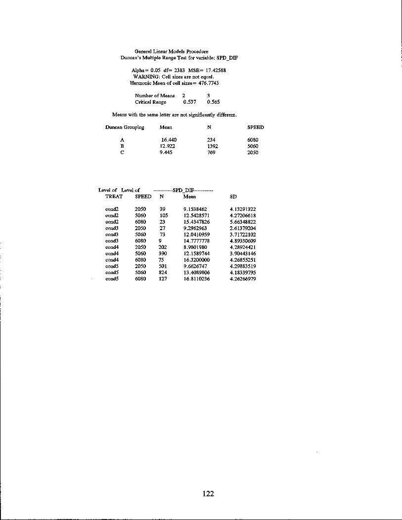
General Linear Models Procedure Duncan's Multiple Range Test for variable: SPD _ DIF
Alpha= 0.05 df= 2383 MSE= 17.42588 WARNING: Cell sizes are not equal.
Harmonic Mean of cell sizes= 476.7743
Number of Means 2 3 Critical Range 0.537 0.565
Means with the same letter are not significantly different.
Duncan Grouping
A B C
Level of Level of TREAT SPEED
cond2 2050 cond2 5060 cond2 6080 cond3 2050 cond3 5060 cond3 6080 cond4 2050 cond4 5060 cond4 6080 cond5 2050 cond5 5060 cond5 6080
Mean
16.440 12.922 9.445
N
234 1392 769
-----------SPD DIF-----------N Mean
39 9.1538462 105 12.5428571 23 15.4347826 27 9.2962963 73 12.0410959 9 14.7777778 202 8.9801980 390 12.1589744 75 16.3200000 501 9.6626747 824 13.4089806 127 16.8110236
122
SD
SPEED
6080 5060 2050
4.13291322 4.27206618 5.66348822 2.61379204 3.71722102 4.89330609 4.28924421 3.90443146 4.26855251 4.29883519 4.18339795 4.26266979

BC(A) [MAIN ANALYSIS]:
General Linear Models Procedure Class Level Information
Class Levels Values
TREAT SPEED
4 3
cond2 2050
cond3 cond4 cond5 5060 6080
Number of observations in data set = 2395
General Linear Models Procedure
Dependent Variable: SPD _DIP
Source DF Sum of Squares Mean Square FValue Pr > F Model 11 3021.63921157 274.69447378 21.37 0.0001 Error 2383 30629.14158175 12.85318572 Corrected Total 2394 33650.78079332
R-Square C.V. RootMSE SPD _DIP Mean 0.089794 55.50353 3.58513399 6.45929019
Source DF Type I SS Mean Square FValue Pr > F
TREAT 3 96.77076696 32.25692232 2.51 0.0571 SPEED 2 2895.93726482 1447.96863241 112.65 0.0001 TREAT*SPEED 6 28.93117979 4.82186330 0.38 0.8952
Source OF Type III SS Mean Square FValue Pr > F
TREAT 3 72.28921525 24.09640508 1.87 0.1317 SPEED 2 955.24944774 477.62472387 37.16 0.0001 TREAT*SPEED 6 28.93117979 4.82186330 0.38 0.8952
123

General Linear Models Procedure Duncan's MUltiple Range Test for variable: SPD _DIF
Alpha= 0.05 df= 2383 MSE= 12.85319 WARNING: Cell sizes are not equal.
Harmonic Mean of cell sizes= 230.5437
Number of Means Critical Range
2 0.663
3 0.698
4 0.720
Means with the same letter are not significantly different.
Duncan Grouping Mean N TREAT
A 6.701 167 cond2 A
B A 6.578 1452 cond5 B A B A 6.228 667 cond4 B B 5.927 109 cond3
General Linear Models Procedure Duncan's Multiple Range Test for variable: SPD _ DIF
Alpha= 0.05 df= 2383 MSE= 12.85319 WARNING: Cell sizes are not equal.
Harmonic Mean of cell sizes= 476.7743
Number of Means Critical Range
2 0.461
3 0.485
Means with the same letter are not significantly different.
Duncan Grouping Mean N SPEED
Level of TREAT
cond2 cond2 cond2 cond3 cond3 cond3 cond4 cond4 cond4 cond5 cond5 cond5
A B C
Level of
8.466 6.920 5.014
234 1392 769
6080 5060 2050
-----------SPD _ DIF----------SPEED N Mean
2050 39 5.43589744 5060 105 6.79047619 6080 23 8.43478261 2050 27 4.51851852 5060 73 6.06849315 6080 9 9.00000000 2050 202 4.62376238 5060 390 6.69230769 6080 75 8.13333333 2050 501 5.16566866 5060 824 7.12014563 6080 127 8.62992126
124
SD
4.84928031 3.53742420 5.69550131 2.02618190 2.88352007 3.53553391 3.29586349 3.21351457 3.25631749 3.70168867 3.69609587 3.81684477

BC(B) [MAIN ANALYSIS]:
General Linear Models Procedure Class Level Information
Class Levels Values
TREAT SPEED
4 3
cond2 2050
cond3 5060
cond4 cond5 6080
Number of observations in data set = 2395
General Linear Models Procedure
Dependent Variable: SPD _DIP Source Model Error Corrected Total
R-Square 0.115793
Source
TREAT SPEED TREAT*SPEED
Source
TREAT SPEED TREAT*SPEED
DF Sum of Squares Mean Square 11 3896.51700690 354.22881881 2383 29754.26378642 12.48605278 2394 33650.78079332
C.V. RootMSE 54.70510 3.53356092
DF Type I SS Mean Square
3 96.77076696 32.25692232 2 3678.75467206 1839.37733603 6 120.99156788 20.16526131
DF Type lli SS Mean Square
3 189.11319533 63.03773178 2 1209.06122375 604.53061188 6 120.99156788 20.16526131
General Linear Models Procedure Duncan's Multiple Range Test for variable: SPD _DIP
Alpha= 0.05 df= 2383 MSE= 12.48605 WARNING: Cell sizes are not equal.
Harmonic Mean of cell sizes= 230.5437
Number of Means Critical Range
2 0.654
3 0.688
4 0.709
Means with the same letter are not significantly different.
Duncan Grouping Mean N
A 6.701 167 A
B A 6.578 1452 B A B A 6.228 667 B B 5.927 109
125
FValue Pr > F 28.37 0.0001
SPD _DIP Mean 6.45929019
FValue Pr > F
2.58 0.0517 147.31 0.0001 1.62 0.1389
FValue Pr > F
5.05 0.0017 48.42 0.0001 1.62 0.1389
TREAT
cond2
cond5
cond4
cond3

General Linear Models Procedure Duncan's Multiple Range Test for variable: SPD _ DIP
Alpha= 0.05 df= 2383 MSE= 12.48605 WARNING: Cell sizes are not equal.
Harmonic Mean of cell sizes= 89.90597
Number of Means 2 3 Critical Range 1.047 1.101
Means with the same letter are not significantly different.
Duncan Grouping
A B C
Mean
11.750 8.127 5.725
N
32 652 1711
Level of Level of -----------SPD DIP-----------TREAT SPEED N Mean
cond2 2050 96 5.6250000 cond2 5060 68 7.9705882 cond2 6080 3 12.3333333 cond3 2050 76 5.2894737 cond3 5060 32 7.5000000 cond3 6080 1 4.0000000 cond4 2050 461 5.5184382 cond4 5060 197 7.7309645 cond4 6080 9 9.6666667 cond5 2050 1078 5.8525046 cond5 5060 355 8.4338028 cond5 6080 19 13.0526316
126
SD
3.45268774 4.80972457 4.61880215 2.42110603 3.55600356
3.27676049 3.20135583 4.03112887 3.61128277 3.63333373 4.71962433
SPEED
6080 5060 2050

MEANS2:
----------------------------------------------------- TREAT = cond2 ------------------------------------------------
MEANS3:
N Obs Variable N Minimum Maximum
167 SPDl SPD2 SPD3
167 39.0000000 65.0000000 167 32.0000000 64.0000000 167 28.0000000 53.0000000
Mean
53.5029940 48.0538922 41.3532934
Std Dev
5.6567203 6.0631789 5.6866763
------------------------------------------------------ TREAT = cond3 ----------------------------------------------------
MEANS4:
N Obs Variable N Minimum Maximum
109 SPDl SPD2 SPD3
109 36.0000000 64.0000000 109 33.0000000 61.0000000 109 30.0000000 57.0000000
Mean
53.0366972 47.3761468 41.4495413
Std Dev
4.8226445 5.2454372 4.8083381
------------------------------------------------------ TREAT = cond4 -----------------------------------------------------
N Obs Variable N Minimum Maximum
MEANS5:
667 SPDl SPD2 SPD3
667 36.0000000 70.0000000 667 32.0000000 63.0000000 667 26.0000000 59.0000000
Mean
52.4527736 47.0164918 40.7886057
Std Dev
5.4512944 5.3902953 5.0491865
---------------------------------------------------- TREAT = cond5 ----------------------------------------------------
N Obs Variable N Minimum Maximum
1452 SPDl SPD2 SPD3
1452 33.0000000 74.0000000 1452 26.0000000 64.0000000 1452 23.0000000 57.0000000
127
Mean
51.9249311 46.0888430 39.5110193
Std Dev
5.5680006 5.6118131 5.1246908

AB [CTR ANALYSIS]:
General Linear Models Procedure Class Level Information
Class
CTR SPEED
Levels
2 2
Number of observations in data set = 154
General Linear Models Procedure
Dependent Variable: SPD _ DIF Source DF Sum of Squares Mean Square Model 3 212.74512987 70.91504329 Error 150 1882.29383117 12.54862554 Corrected Total 153 2095.03896104
R-Square C.V. RootMSE 0.101547 56.12451 3.54240392
Source DF Type I SS Mean Square CTR 1 0.60800866 0.60800866 SPEED 1 211.33587196 211.33587196 CTR*SPEED 1 0.80124925 0.80124925
Source DF Type III SS Mean Square CTR 1 2.16737981 2.16737981 SPEED 1 189.01316978 189.01316978 CTR*SPEED 1 0.80124925 0.80124925
General Linear Models Procedure
Values
of on 5160 6080
FValue 5.65
FValue 0.05 16.84 0.06
FValue 0.17 15.06 0.06
Duncan's Multiple Range Test for variable: SPD _DIF
AJpha= 0.05 df= 150 MSE= 12.54863 WARNING: Cell sizes are not equal.
Harmonic Mean of cell sizes= 76.36364
Number of Means Critical Range
2 1.139
Means with the same letter are not significantly different.
Duncan Grouping
A A A
Mean
6.369
6.243
N CTR
84 of
70 on
128
Pr > F 0.0011
SPD _DIF Mean 6.31168831
Pr > F 0.8261 0.0001 0.8009
Pr > F 0.6783 0.0002 0.8009

,--~~~--~~~~~------- ----
General Linear Models Procedure Duncan's Multiple Range Test for variable: SPD _ DIF
AJpha= 0.05 df= 150 MSE= 12.54863 WARNING: Cell sizes are not equal.
Harmonic Mean of cell sizes= 36.27273
Number of Means Critical Range
2 1.652
Means with the same letter are not significantly different.
Duncan Grouping Mean N SPEED
A B
Level of CTR
of of on on
9.190 5.857
21 133
6080 5160
Level of -----------SPD DIF----------SPEED N Mean
5160 77 6.10389610 6080 7 9.28571429 5160 56 5.51785714 6080 14 9.14285714
129
SD
3.45110362 4.23140188 3.58781307 3.52697610

AB [eTR ANALYSIS, SPEED=HIGH]:
General Linear Models Procedure Class Level Information
Class CTR
Levels 2
Values of on
Number of observations in data set = 21
General Linear Models Procedure
Dependent Variable: SPD_DIF Source Model Error Corrected Total
Source CTR Source CTR
DF Sum of Squares Mean Square 1 0.09523810 0.09523810 19 269.14285714 14.16541353 20 269.23809524
R-Square C.V. RootMSE 0.000354 40.95214 3.76369679
DF Type ISS Mean Square 1 0.09523810 0.09523810 DF TypeillSS Mean Square 1 0.09523810 0.09523810
General Linear Models Procedure Duncan's Multiple Range Test for variable: SPD _ DIF
Alpha= 0.05 df= 19 MSE= 14.16541 WARNING: Cell sizes are not equal.
Harmonic Mean of cell sizes= 9.333333
Number of Means 2 Critical Range 3.641
Means with the same letter are not significantly different.
Duncan Grouping
A A A
Mean
9.286
9.143
N CTR
7 of
14 on
130
FValue Pr > F 0.01 0.9355
SPD _DIF Mean 9.19047619
FValue Pr > F 0.01 0.9355 FValue Pr > F 0.01 0.9355

AB [CTR ANALYSIS, SPEED = LOW]:
General Linear Models Procedure Class Level Information
Class CTR
Levels 2
Values of on
Number of observations in data set = 133
General Linear Models Procedure
Dependent Variable: SPD_DIF
Source Model Error Corrected Total
R-Square 0.006855
Source CTR
Source CTR
DF Sum of Squares Mean Square 1 11.13474026 11.13474026 131 1613.15097403 12.31412957 132 1624.28571429
C.V. RootMSE 59.91231 3.50914941
DF Type I SS Mean Square 1 11.13474026 11.13474026
DF TypeillSS Mean Square 1 11.13474026 11.13474026
General Linear Models Procedure Duncan's MUltiple Range Test for variable: SPD _ DIF
Alpha= 0.05 df= 131 MSE= 12.31413 WARNING: Cell sizes are not equal.
Harmonic Mean of cell sizes= 64.84211
Number of Means 2 Critical Range 1.224
Means with the same letter are not significantly different.
Duncan Grouping
A A A
Mean
6.104
5.518
N CTR
77 of
56 on
131
FValue Pr > F 0.90 0.3434
SPD DIFMean 5.85714286
FValue Pr > F 0.90 0.3434
FValue Pr > F 0.90 0.3434

AC [CTR ANALYSIS]:
General Linear Models Procedure Class Level Information
Class CTR
Levels 2
Values of on
Number of observations in data set = 197
General Linear Models Procedure
Dependent Variable: SPD_DIF Source Model Error Corrected Total
R-Square 0.058470
Source CTR
Source CTR
DF Sum of Squares Mean Square 1 173.13843238 173.13843238 195 2787.98847118 14.29737678 196 2961.12690355
C.V. RootMSE 30.60369 3.78118722
DF TypeISS Mean Square 1 173.13843238 173.13843238
DF Type lli SS Mean Square 1 173.13843238 173.13843238
General Linear Models Procedure Duncan's Multiple Range Test for variable: SPD _DIF
Alpha= 0.05 df= 195 MSE= 14.29738 WARNING: Cell sizes are not equal.
Harmonic Mean of cell sizes= 81.01523
Number of Means 2 Critical Range 1.180
Means with the same letter are not significantly different.
Duncan Grouping
A B
Mean
13.825 11.757
N
57 140
132
CTR
on of
FValue Pr > F 12.11 0.0006
SPD _DIF Mean 12.35532995
FValue Pr > F 12.11 0.0006
FValue Pr > F 12.11 0.0006

Be [CTR ANALYSIS]:
General Linear Models Procedure Class Level Information
Class CTR
Levels 2
Values of on
Number of observations in data set = 122
General Linear Models Procedure
Dependent Variable: SPD_DIF
Source Model Error Corrected Total
Source CTR
Source CTR
DF Sum of Squares Mean Square 1 61.55975532 61.55975532 120 1314.41565452 10.95346379 121 1375.97540984
R-Square C.V. RootMSE 0.044739 44.51725 3.30960176
DF TypeISS Mean Square 1 61.55975532 61.55975532
DF Type III SS Mean Square 1 61.55975532 61.55975532
General Linear Models Procedure Duncan's Multiple Range Test for variable: SPD _ DIF
Alpha= 0.05 df= 120 MSE= 10.95346 WARNING: Cell sizes are not equal.
Harmonic Mean of cell sizes= 60.7377
Number of Means 2 Critical Range 1.193
Means with the same letter are not significantly different.
Duncan Grouping
A B
Mean
8.193 6.769
N
57 65
133
CTR
on of
FValue Pr > F 5.62 0.0193
SPD _ DIF Mean 7.43442623
FValue Pr > F 5.62 0.0193
FValue Pr > F 5.62 0.0193
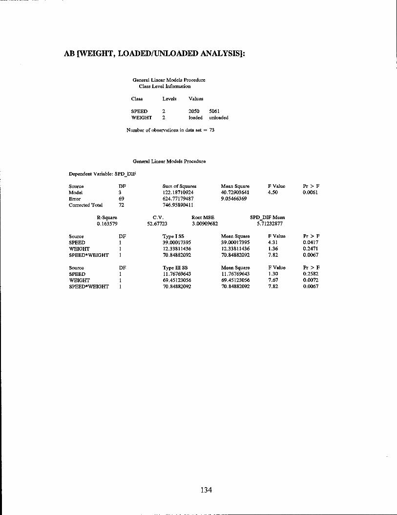
AB [WEIGHT, LOADED/UNLOADED ANALYSIS]:
General Linear Models Procedure Class Level Information
Class
SPEED WEIGHT
Levels
2 2
Values
2050 5061 loaded unloaded
Number of observations in data set = 73
General Linear Models Procedure
Dependent Variable: SPD _DIP
Source DF Sum of Squares Mean Square Model 3 122.18710924 40.72903641 Error 69 624.77179487 9.05466369 Corrected Total 72 746.95890411
R-Square C.V. RootMSE 0.163579 52.67723 3.00909682
Source DF Type I SS Mean Square SPEED 1 39.00017395 39.00017395 WEIGHT 1 12.33811436 12.33811436 SPEED*WEIGHT 1 70.84882092 70.84882092
Source DF Type III SS Mean Square SPEED 1 11.76769643 11.76769643 WEIGHT 1 69.45123056 69.45123056 SPEED*WEIGHT 1 70.84882092 70.84882092
134
FValue Pr > F 4.50 0.0061
SPD _DIP Mean 5.71232877
FValue Pr > F 4.31 0.0417 1.36 0.2471 7.82 0.0067
FValue Pr > F 1.30 0.2582 7.67 0.0072 7.82 0.0067

~~~~~~--~~------
General Linear Models Procedure Duncan's Multiple Range Test for variable: SPD _ DIF
Alpha= 0.05 df= 69 MSE= 9.054664 WARNING: Cell sizes are not equal.
Hannonic Mean of cell sizes= 34.52055
Number of Means 2 Critical Range 1.446
Means with the same letter are not significantly different.
Duncan Grouping
A B
Mean
6.289 4.786
N
45 28
General Linear Models Procedure
SPEED
5061 2050
Duncan's Multiple Range Test for variable: SPD _ DIF
Alpha= 0.05 df= 69 MSE= 9.054664 WARNING: Cell sizes are not equal.
Hannonic Mean of cell sizes= 26.08219
Number of Means 2 Critical Range 1.664
Means with the same letter are not significantly different.
Duncan Grouping
Level of SPEED
2050 2050 5061 5061
A A A
Level of WEIGHT
loaded unloaded loaded unloaded
Mean N WEIGHT
6.824 17 unloaded
5.375 56 loaded
-----------SPD DIF-----------N Mean SD
26 4.3076923 3.03010535 2 11.0000000 1.41421356 30 6.3000000 3.16391290 15 6.2666667 2.71152742
135

AB [WADED/UNLOADED, SPEED=HIGH]:
General Linear Models Procedure Class Level Information
Class Levels Values
WEIGHT 2 loaded unloaded
Number of observations in data set = 45
General Linear Models Procedure
Dependent Variable: SPD _DIP Source Model Error Corrected Total
R-Square 0.000028
Source WEIGHT
Source WEIGHT
DF Sum of Squares Mean Square I 0.01111111 0.01111111 43 393.23333333 9.14496124 44 393.24444444
C.V. RootMSE 48.08582 3.02406370
DF TypeJ SS Mean Square 1 0.01111111 0.01111111
DF TypeillSS Mean Square 1 0.01111111 0.01111111
General Linear Models Procedure Duncan's Multiple Range Test for variable: SPD _DIP
Alpha= 0.05 df= 43 MSE= 9.144961 WARNING: Cell sizes are not equal. Harmonic Mean of cell sizes= 20
Number of Means 2 Critical Range 1.929
Means with the same letter are not significantly different.
Duncan Grouping
A A A
Mean
6.300
6.267
N WEIGHT
30 loaded
15 unloaded
136
FValue 0.00
SPD _DIP Mean 6.28888889
FValue 0.00
FValue 0.00
Pr > F 0.9724
Pr > F 0.9724
Pr > F 0.9724
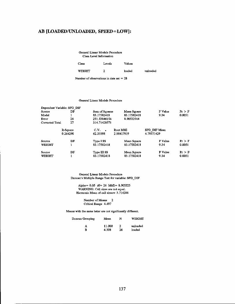
AB [LOADED/UNLOADED, SPEED=LOW]:
General Linear Models Procedure Class Level Information
Class Levels
WEIGHT 2
Values
loaded
Number of observations in data set = 28
General Linear Models Procedure
Dependent Variable: SPD_DIP Source Model Error Corrected Total
Source WEIGHT
Source WEIGHT
DF Sum of Squares Mean Square 1 83.17582418 83.17582418 26 231.53846154 8.90532544 27 314.71428571
R-Square C.V. RootMSE 0.264290 62.35598 2.98417919
DF Type I SS Mean Square 1 83.17582418 83.17582418
DF Type ill SS Mean Square 1 83.17582418 83.17582418
General Linear Models Procedure Duncan's Multiple Range Test for variable: SPD _DIP
AIpha= 0.05 df= 26 MSE= 8.905325 WARNING: Cell sizes are not equal.
Harmonic Mean of cell sizes = 3.714286
Number of Means 2 Critical Range 4.497
Means with the same letter are not significantly different.
Duncan Grouping
A B
Mean
11.000 4.308
N
2 26
137
WEIGHT
unloaded loaded
unloaded
FValue Pr > F 9.34 0.0051
SPD_DIPMean 4.78571429
FValue Pr > F 9.34 0.0051
FValue Pr > F 9.34 0.0051

AB [TRAILER TYPE ANALYSIS]:
General Linear Models Procedure Class Level Information
Class Levels Values
TYPE 3 FLTUNKVAN
Number of observations in data set = 72
General Linear Models Procedure
Dependent Variable: SPD_DIF Source Model Error Corrected Total
R-Square 0.028956
Source TYPE Source TYPE
DF Sum of Squares Mean Square 2 21.61436926 10.80718463 69 724.83007519 10.50478370 71 746.44444444
C.V. RootMSE 56.64073 3.24110841
DF TypeISS Mean Square 2 21.61436926 10.80718463 DF TypeillSS Mean Square 2 21.61436926 10.80718463
General Linear Models Procedure Duncan I s Multiple Range Test for variable: SPD _DIP
Alpha= 0.05 df= 69 MSE= 10.50478 WARNING: Cell sizes are not equal.
Harmonic Mean of cell sizes= 20.30534
Number of Means Critical Range
2 2.031
3 2.136
Means with the same letter are not significantly different.
Duncan Grouping Mean N TYPE
A 6.211 38 VAN A A 5.400 20 FLT A A 4.857 14 UNK
138
FValue Pr > F 1.03 0.3629
SPD DIFMean 5.72222222
FValue Pr > F 1.03 0.3629 FValue Pr > F 1.03 0.3629

AB [CENTER OF GRAVITY ANALYSIS]:
General Linear Models Procedure Class Level Information
Class Levels Values
CENTGRA V 3 high low unkn
Number of observations in data set = 72
NOTE: Due to missing values, only 71 observations can be used in this analysis.
General Linear Models Procedure
Dependent Variable: SPD_DIP Source Model Error Corrected Total
R-Square 0.041597
Source CENTGRAV
Source CENTGRAV
DF Sum of Squares Mean Square 2 31.02813032 15.51406516 68 714.88736264 10.51304945 70 745.91549296
C.V. RootMSE 56.56246 3.24238330
DF TypeISS Mean Square 2 31.02813032 15.51406516
DF TypeillSS Mean Square 2 31.02813032 15.51406516
General Linear Models Procedure Duncan's Multiple Range Test for variable: SPD _DIP
A1pha= 0.05 df= 68 MSE= 10.51305 WARNING: Cell sizes are not equal.
Harmonic Mean of cell sizes= 17.53577
Number of Means Critical Range
2 2.187
3 2.300
Means with the same letter are not significantly different.
Duncan Grouping Mean N CENTGRAV
A 6.250 44 high A A 4.923 13 low A A 4.857 14 unkn
139
FValue 1.48
SPD _DIP Mean 5.73239437
FValue 1.48
FValue 1.48
Pr > F 0.2358
Pr > F 0.2358
Pr > F 0.2358

AB [COMBINATION TRUCKS ANALYSIS]:
General Linear Models Procedure Class Level Information
Class
TREAT SPEED
Levels
4 3
Values
cond2 2050
cond3 5060
Number of observations in data set = 1622
General Linear Models Procedure
cond4 cond5 6080
Dependent Variable: SPD _ DIF Source Model Error Corrected Total
R-Square 0.089024
Source TREAT SPEED TREAT*SPEED
Source TREAT SPEED TREAT*SPEED
DF Sum of Squares Mean Square FValue 11 1694.81518750 154.07410795 14.30 1610 17342.90861028 10.77199293 1621 19037.72379778
C.V. RootMSE SPD DIFMean 37.27910 3.28207144 5.72996301
DF Type I SS Mean Square 3 140.10169915 46.70056638 2 1414.40058444 707.20029222 6 140.31290391 23.38548398
DF Type ill SS Mean Square 3 133.35203623 44.45067874 2 241.32023216 120.66011608 6 140.31290391 23.38548398
General Linear Models Procedure Duncan's Multiple Range Test for variable: SPD _ DIF
Alpha= 0.05 df= 1610 MSE= 10.77199 WARNING: Cell sizes are not equal.
Harmonic Mean of cell sizes= 121.8126
Number of Means Critical Range
2 0.835
3 0.879
4 0.906
FValue 4.34 65.65 2.17
FValue 4.13 11.20 2.17
Means with the same letter are not significantly different.
Duncan Grouping Mean N TREAT
A 5.942 1045 cond5 A A 5.614 83 cond2 A A 5.456 57 cond3 A A 5.281 437 cond4
General Linear Models Procedure
Duncan's Multiple Range Test for variable: SPD _DIF
140
Pr > F 0.0001
Pr > F 0.0047 0.0001 0.0432
Pr > F 0.0063 0.0001 0.0432

Alpha= 0.05 df= 1610 MSE= 10.77199 WARNING: Cell sizes are not equal.
Harmonic Mean of cell sizes = 311.5292
Number of Means Critical Range
2 0.522
3 0.549
Means with the same letter are not significantly different.
Duncan Grouping
A B C
Level of Level of TREAT SPEED
cond2 2050 cond2 5060 cond2 6080 cond3 2050 cond3 5060 cond3 6080 cond4 2050 cond4 5060 cond4 6080 cond5 2050 cond5 5060 cond5 6080
N
19 55 9 18 35 4 117 268 52 370 590 85
Mean
7.860 5.977 4.674
N
150 948 524
SPEED
6080 5060 2050
-----------SPD DIF----------Mean SO
4.73684211 3.24623038 5.67272727 2.86132930 7.11111111 2.75882423 4.33333333 2.40098019 5.97142857 3.04365989 6.00000000 2.00000000 4.77777778 2.47438990 5.11940299 2.93894112 7.25000000 2.76444513 4.65405405 3.69857473 6.39491525 3.41846200 8.40000000 3.25210555
141
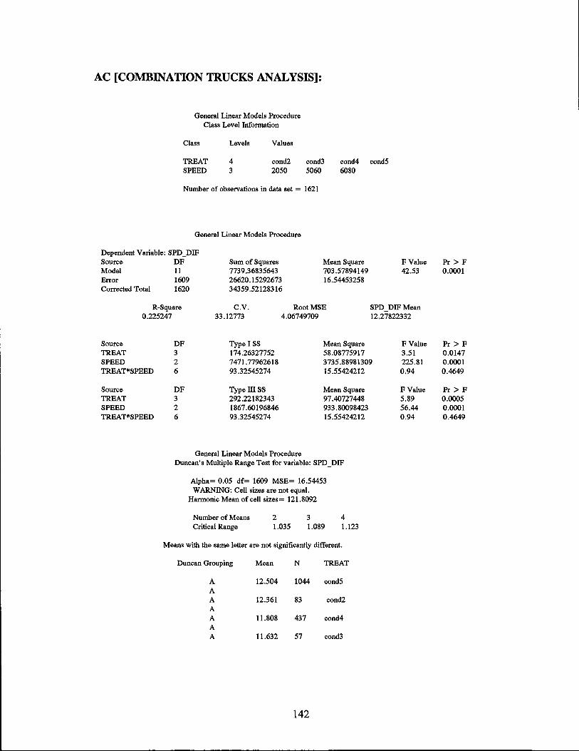
AC [COMBINATION TRUCKS ANALYSIS]:
General Linear Models Procedure Class Level Information
Class
TREAT SPEED
Levels
4 3
Values
cond2 2050
cond3 5060
cond4 cond5 6080
Number of observations in data set = 1621
General Linear Models Procedure
Dependent Variable: SPD_DIP Source DF Sum of Squares Mean Square Model 11 7739.36835643 703.57894149 Error 1609 26620.15292673 16.54453258 Corrected Total 1620 34359.52128316
FValue 42.53
R-8quare C.V. RootMSE SPD DIPMean 0.225247 33.12773 4.06749709 12.27822332
Source DF Type I SS Mean Square FValue TREAT 3 174.26327752 58.08775917 3.51 SPEED 2 7471.77962618 3735.88981309 225.81 TREAT*SPEED
Source TREAT SPEED TREAT*SPEED
6 93.32545274 15.55424212
DF Type III SS Mean Square 3 292.22182343 97.40727448 2 1867.60196846 933.80098423 6 93.32545274 15.55424212
General Linear Models Procedure Duncan's Multiple Range Test for variable: SPD _DIP
Alpha= 0.05 df= 1609 MSE= 16.54453 WARNING: Cell sizes are not equal.
Harmonic Mean of cell sizes= 121.8092
Number of Means Critical Range
2 1.035
3 1.089
4 1.123
Means with the same letter are not significantly different.
Duncan Grouping Mean N TREAT
A 12.504 1044 cond5 A A 12.361 83 cond2 A A 11.808 437 cond4 A A 11.632 57 cond3
142
0.94
FValue 5.89 56.44 0.94
Pr > F 0.0001
Pr > F 0.0147 0.0001 0.4649
Pr > F 0.0005 0.0001 0.4649

General Linear Models Procedure Duncan's Multiple Range Test for variable: SPD _DIP
Alpha= 0.05 df= 1609 MSE= 16.54453 WARNING: Cell sizes are not equal.
Harmonic Mean of cell sizes = 311.4112
Number of Means Critical Range
2 0.648
3 0.681
Means with the same letter are not significantly different.
Duncan Grouping
A B C
Mean
16.880 12.991 9.667
N
150 948 523
SPEED
6080 5060 2050
Level of Level of -----------SPD DIP--------TREAT SPEED N Mean
cond2 2050 19 9.4736842 cond2 5060 55 12.6727273 cond2 6080 9 16.5555556 cond3 2050 18 9.1666667 cond3 5060 35 12.3142857 cond3 6080 4 16.7500000 cond4 2050 117 9.4444444 cond4 5060 268 12.0858209 cond4 6080 52 15.6923077 cond5 2050 369 9.7723577 cond5 5060 590 13.4711864 cond5 6080 85 17.6470588
143
SD
3.30602852 3.82513396 5.81186526 2.83362167 3.80225497 5.31507291 3.70098879 3.62111273 3.42733225 4.38217674 4.19859508 4.24181532

BC(A) [COMBINATION TRUCKS ANALYSIS]:
General Linear Models Procedure Class Level Information
Class TREAT SPEED
Levels 4 3
Values cond2 2050
cond3 5060
Number of observations in data set = 1621
General Linear Models Procedure
cond4 6080
Dependent Variable: SPD _DIP Source DF Sum of Squares Mean Square Model 11 2464.56759302 224.05159937 Error 1609 21515.16590482 13.37176253 Corrected Total 1620 23979.73349784
R-Square C.V. RootMSE 0.102777 55.85732 3.65674206
Source TREAT SPEED TREAT*SPEED
Source TREAT SPEED TREAT*SPEED
DF Type I SS Mean Square 3 11.53576073 3.84525358 2 2411.09492011 1205.54746006 6 41.93691218 6.98948536
DF TypeillSS Mean Square 3 41.67746917 13.89248972 2 767.07552902 383.53776451 6 41.93691218 6.98948536
General Linear Models Procedure Duncan's Multiple Range Test for variable: SPD _DIP
Alpha= 0.05 df= 1609 MSE= 13.37176 WARNING: Cell sizes are not equal.
Harmonic Mean of cell sizes= 121.8092
Number of Means Critical Range
2 0.931
3 0.979
4 1.010
Means with the same letter are not significantly different.
Duncan Grouping Mean N TREAT
A 6.747 83 cond2 A A 6.559 1044 cond5 A A 6.526 437 cond4 A A 6.175 57 cond3
144
cond5
FValue Pr> F 16.76 0.0001
SPD _DIP Mean 6.54657619
FValue Pr > F 0.29 0.8344 90.16 0.0001 0.52 0.7915
FValue Pr > F 1.04 0.3743 28.68 0.0001 0.52 0.7915

General Linear Models Procedure Duncan's Multiple Range Test for variable: SPD _DIP
Alpha= 0.05 df= 1609 MSE= 13.37176 WARNING: Cell sizes are not equal.
Harmonic Mean of cell sizes = 311.4112
Number of Means Critical Range
2 0.582
3 0.612
Means with the same letter are not significantly different.
Duncan Grouping
A B C
Level of Level of TREAT SPEED
cond2 2050 cond2 5060 cond2 6080 cond3 2050 cond3 5060 cond3 6080 cond4 2050 cond4 5060 cond4 6080 cond5 2050 cond5 5060 cond5 6080
Mean
9.020 7.014 4.990
N
150 948 523
SPEED
6080 5060 2050
-----------SPD DIF-----------N Mean SD
19 4.7368421 4.47017406 55 7.0000000 3.33888427 9 9.4444444 6.02310367 18 4.8333333 1.97781817 35 6.3428571 3.08643004 4 10.7500000 4.11298756 117 4.6666667 3.08220700 268 6.9664179 3.16150640 52 8.4423077 3.20179767 369 5.1138211 3.86428023 590 7.0762712 3.88667302 85 9.2470588 3.67716856
145

BC(B) [COMBINATION TRUCKS ANALYSIS]:
General Linear Models Procedure Class Level Information
Class TREAT SPEED
Levels 4 3
Values cond2 2050
cond3 5060
Number of observations in data set = 1621
General Linear Models Procedure
cond4 cond5 6080
Dependent Variable: SPD_DIP Source DF Sum of Squares Mean Square Model 9 2887.44154036 320.82683782 Error 1611 21092.29195748 13.09267036 Corrected Total 1620 23979.73349784
R-Square C.V. RootMSE SPD_DIPMean 0.120412 55.27133 3.61837952 6.54657619
Source TREAT SPEED TREAT*SPEED
Source TREAT SPEED TREAT*SPEED
OFI Type ISS Mean Square 3 11.53576073 3.84525358 2 2830.37485630 1415.18742815 4 45.53092332 11.38273083
DF Type III SS Mean Square 3 37.23921927 12.41307309 2 902.93243913 451.46621957 4 45.53092332 11.38273083
General Linear Models Procedure Duncan's Multiple Range Test for variable: SPD _DIP
Alpha= 0.05 df= 1611 MSE= 13.09267 WARNING: Cell sizes are not equal.
Harmonic Mean of cell sizes= 121.8092
Number of Means Critical Range
2 0.921
3 0.969
4 0.999
Means with the same letter are not significantly different.
Duncan Grouping Mean N TREAT
A 6.747 83 cond2 A A 6.559 1044 cond5 A A 6.526 437 cond4 A A 6.175 57 cond3
146
FValue Pr > F 24.50 0.0001
FValue Pr > F 0.29 0.8300 108.09 0.0001 0.87 0.4815
FValue Pr> F 0.95 0.4165 34.48 0.0001 0.87 0.4815

General Linear Models Procedure Duncan's Multiple Range Test for variable: SPD _ DIF
A1pha= 0.05 df= 1611 MSE= 13.09267 WARNING: Cell sizes are not equal.
Harmonic Mean of cell sizes= 37.49388
Number of Means Critical Range
2 1.660
3 1.746
Means with the same letter are not significantly different.
Duncan Grouping
A B C
Mean
12.385 8.445 5.745
N
13 449 1159
SPEED
6080 5060 2050
Level of Level of -----------SPD _ DIF-----------TREAT SPEED N Mean
cond2 2050 53 6.0566038 cond2 5060 30 7.9666667 cond3 2050 41 5.4390244 cond3 5060 16 8.0625000 cond4 2050 283 5.6360424 cond4 5060 150 8.1000000 cond4 6080 4 10.5000000 cond5 2050 782 5.7800512 cond5 5060 253 8.7312253 cond5 6080 9 13.2222222
147
SD
3.99718696 4.13965960 2.30270255 4.21851080 3.12591114 3.15749880 3.69684550 3.76726394 3.77529738 6.39878461