A proposal to the NSF Design of Experiments …s Null Hypothesis Testing 1. Set up a statistical...

ESD.86Hypothesis Testing

Dan FreyAssociate Professor of Mechanical Engineering and Engineering Systems

Gigerenzer's Paper

• "Mindless Statistics"• Journal of Socio-Economics• What are its key points?

– History– Research practices– Statistics per se

Gigerenzer, G., 2004,“Mindless Statistics,” J. of Socio-Economics 33:587-606.

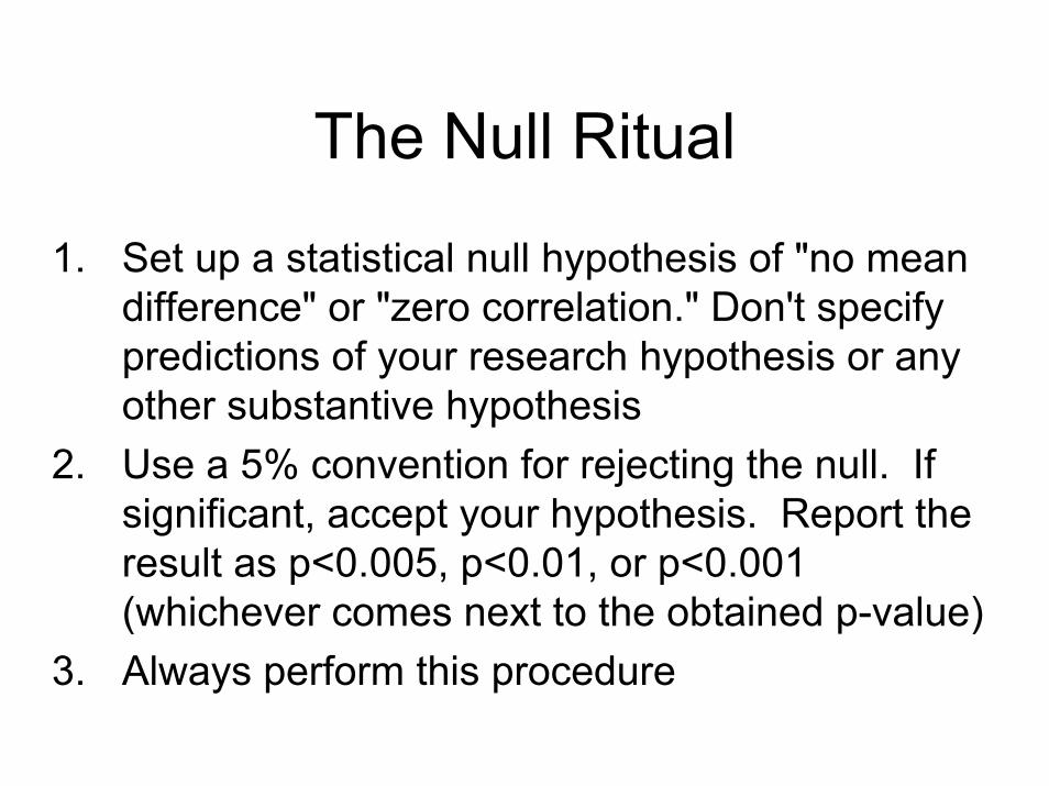
The Null Ritual

1. Set up a statistical null hypothesis of "no mean difference" or "zero correlation." Don't specify predictions of your research hypothesis or any other substantive hypothesis

2. Use a 5% convention for rejecting the null. If significant, accept your hypothesis. Report the result as p<0.005, p<0.01, or p<0.001 (whichever comes next to the obtained p-value)

3. Always perform this procedure

Is This Really Being Done?• Quick check – Compendex search for "significant" in

abstract and the title of a research journal I read, publish in, review for

• 11 results in 2006, 12 in 2005, etc.

Chusilp, P., and Y. Jin, 2006, "Impact of Mental Iteration on Concept Generation," ASME J. of Mech. Design 128:14-25.

The paper's conclusion section states: "The results suggested that (1) increasing number of iteration has positive impact on quality, variety, and quantity, but mixed effect on novelty..."

Copyright © 2006 by ASME. Used with permission.

Fisher's Null Hypothesis Testing

1. Set up a statistical null hypothesis. The null need not be a nil hypothesis (i.e., zero difference).

2. Report the exact level of significance ... Do not use a conventional 5% level, and do not talk about accepting or rejecting hypotheses.

3. Use this procedure only if you know very little about the problem at hand.

Test for "Goodness of Fit"as Conducted in Weibull's Paper

• Calculates the degrees of freedom10 (bins) -1 – 3 (parameters of the df) = 6

• Calculates the statistic• States the P-value • Comparison to alternative

∑ −=

estimatedestimatedobserved 2

2 )(χ

Note: Table is cumulative, χ2test requires frequency in bin

P=0.49 for Weibull

0 10 200

0.1

0.2

dchisq x 6,( )

0

0.2⎛⎜⎝

⎞⎟⎠

0

0.2⎛⎜⎝

⎞⎟⎠

x5.40

5.40⎛⎜⎝

⎞⎟⎠

,18.17

18.17⎛⎜⎝

⎞⎟⎠

,

P=0.008for Normal

From the previous lecture


Gigernezer's Quiz

1. You have absolutely disproved the null hypothesis2. You have found the probability of the null hypothesis being true.3. You have absolutely proved your experimental hypothesis (that

there is a difference between the population means).4. You can deduce the probability of the experimental hypothesis

being true.5. You know, if you decide to reject the null hypothesis, the

probability that you are making the wrong decision.6. You have a reliable experimental finding in the sense that if,

hypothetically, the experiment were repeated a great number of times, you would obtain a significant result on 99% of occasions.

Suppose you have a treatment that you suspect may alter performance on a certain task. You compare the means of your control and experimental groups (say 20 subjects in each sample). Further, suppose you use a simple independent means t-test and your result is significant (t = 2.7, d.f. = 18, p = 0.01). Please mark each of the statements below as “true” or “false.” ...

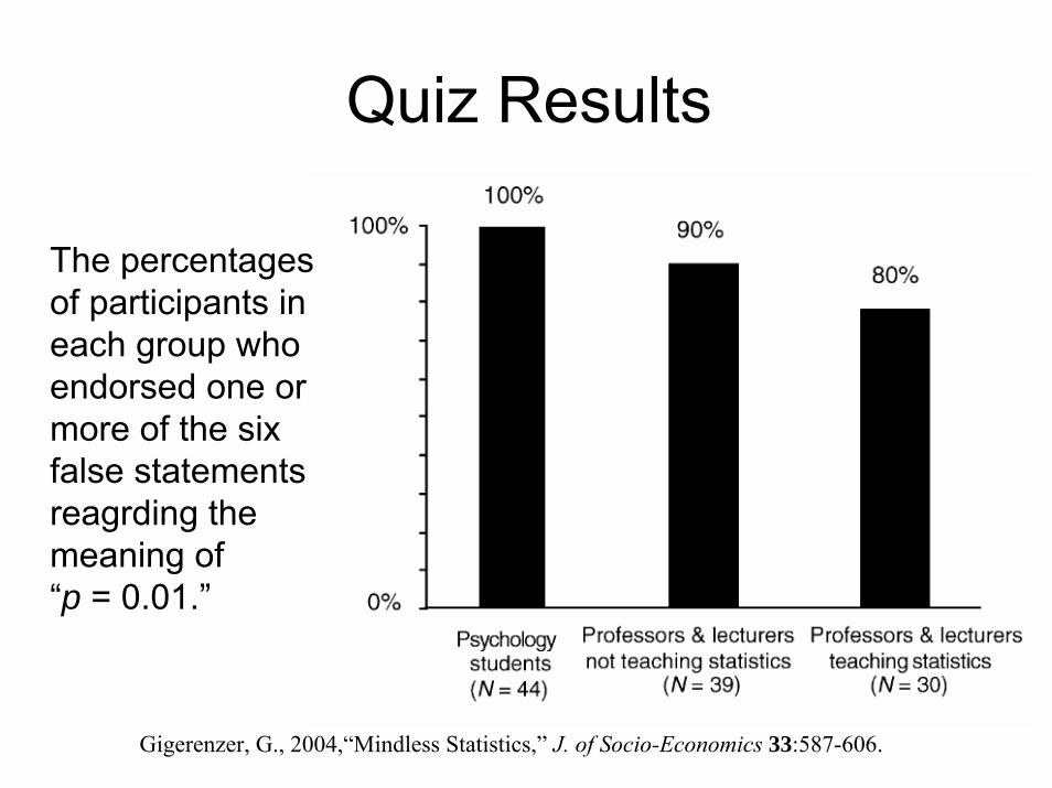
Quiz Results

The percentages of participants in each group who endorsed one or more of the six false statements reagrding the meaning of “p = 0.01.”


Matlab's Description of theTwo-sample t-test

h = ttest2(x,y) performs a t-test of the null hypothesis that data in the vectors x and y are independent random samples from normal distributions with equal means and equal but unknown variances, against the alternative that the means are not equal. The result of the test is returned in h. h = 1 indicates a rejection of the null hypothesis at the 5% significance level. h = 0 indicates a failure to reject the null hypothesis at the 5% significance level.

Concept Question• This Matlab code repreatedly generates and tests

simulated "data" • 20 "subjects" in the control and treatment groups• Both normally distributed with the same mean• How often will the t-test reject H0 (α=0.01)?

for i=1:1000control=random('Normal',0,1,1,20);trt=random('Normal',0,1,1,20);reject_null(i) = ttest2(control,trt,0.01);

endmean(reject_null)

1) ~99% of the time2) ~1% of the time3) ~50% of the time4) None of the above

Concept Question• This Matlab code repreatedly generates and tests

simulated "data" • 20 "subjects" in the control and treatment groups• Both normally distributed with the different means• How often will the t-test reject H0 (α=0.01)?

for i=1:1000control=random('Normal',0,1,1,200);trt= random('Normal',1,1,1,200);reject_null(i) = ttest2(control,trt,0.01);


1) ~99% of the time2) ~1% of the time3) ~50% of the time4) None of the above

Concept Question• How do “effect” and "alpha" affect the rate

at which the t-test rejects H0 ?

a) ↑ effect, ↑ rejectsb) ↑ effect, ↓ rejectsc) ↑ alpha, ↑ rejectsd) ↑ alpha, ↓ rejects

1) a & c2) a & d3) b & c4) b & d

effect=1;alpha=0.01;for i=1:1000

control=random('Normal',0,1,1,20);trt= random('Normal',effect,1,1,20);reject_null(i) = ttest2(control,trt,alpha);


What if Assumptions are Violated?• This Matlab code generates data with a

no treatment effect on mean• But dispersion is affected by treatment • Type I error rate rises

for i=1:1000control=random('Normal',0,1,1,20);trt=random('Normal',0,2,1,20);reject_null(i) = ttest2(control,trt,0.01);


What if Assumptions are Violated?• This Matlab code generates data with a

no treatment effect on mean• The two poulations are uniformly dist. • Type I error rate rises

for i=1:1000control=random('Uniform',0,1,1,20);trt=random('Uniform',0,1,1,20);reject_null(i) = ttest2(control,trt,0.01);


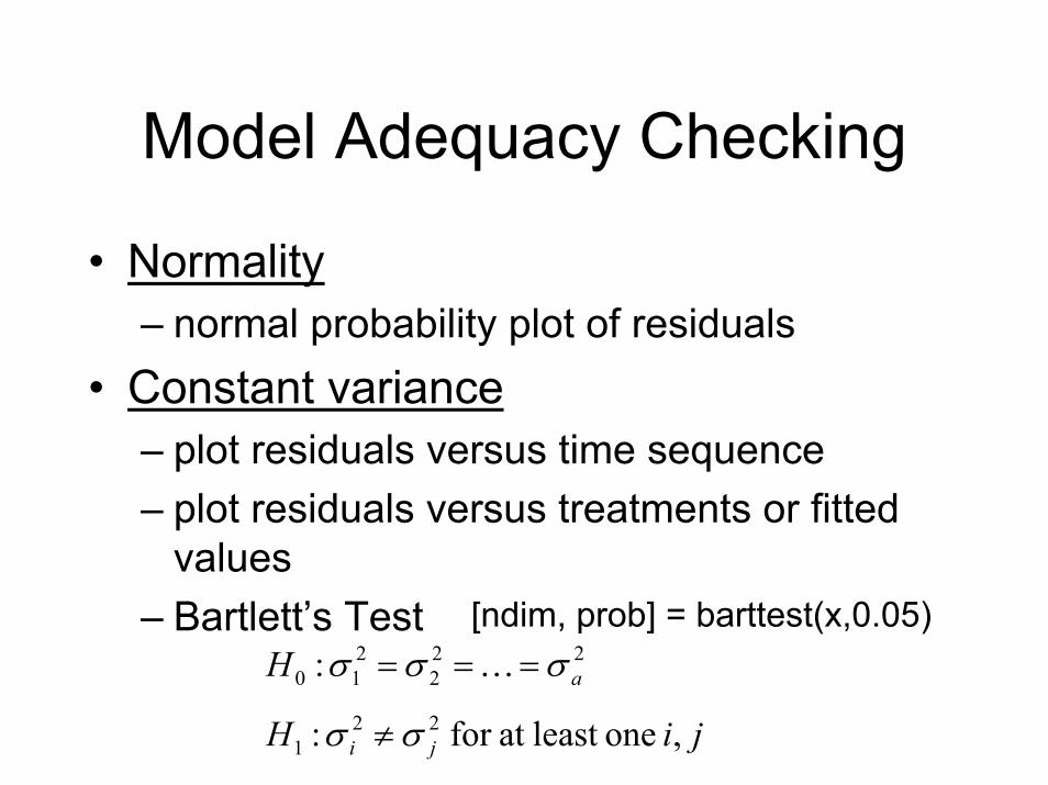
Model Adequacy Checking

• Normality– normal probability plot of residuals

• Constant variance– plot residuals versus time sequence– plot residuals versus treatments or fitted

values– Bartlett’s Test [ndim, prob] = barttest(x,0.05)

jiH

H

ji

a

, oneleast at for :

:22

1

222

210

σσ

σσσ

≠

=== K

Randomization Distribution• The null hypothesis implies that the observations

are not a function of the treatments• If that were true, the allocation of the data to

treatments (rows) shouldn’t affect the test statistic• How likely is the statistic observed under re-

ordering? Observations

Cotton weight

percentage 1 2 3 4 515 7 7 15 11 920 12 17 12 18 1825 14 18 18 19 1930 19 25 22 19 2335 7 10 11 15 11

Randomization Distribution• This code reorders

the data from the cotton experiment

• Does the ANOVA• Repeats 5000

times• Plots the pdf of the

F ratio

trials=5000;bins=trials/100;X=[7 7 15 11 9 12 17 12 18 18 14 18 1819 19 19 25 22 19 23 7 10 11 15 11];group=ceil([1:25]/5);[p,table,stats] = anova1(X, group,'off');F=cell2mat(table(2,5))

for i=1:trialsr=rand(1,25);[B,INDEX] = sort(r);Xr(1:25)=X(INDEX);[p,table,stats] = anova1(Xr, group,'off');Fratio(i)=cell2mat(table(2,5));

end

hold off[n,x] = hist(Fratio,bins);n=n/(trials*(x(2)-x(1)));colormap hsvbar(x,n)hold on

xmax=max(Fratio);x=0:(xmax/100):xmax;y = fpdf(x,4,20);plot(x,y,'LineWidth',2)

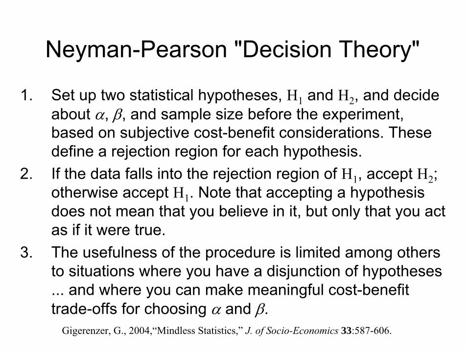
Neyman-Pearson "Decision Theory"

1. Set up two statistical hypotheses, H1 and H2, and decide about α, β, and sample size before the experiment, based on subjective cost-benefit considerations. These define a rejection region for each hypothesis.

2. If the data falls into the rejection region of H1, accept H2; otherwise accept H1. Note that accepting a hypothesis does not mean that you believe in it, but only that you act as if it were true.

3. The usefulness of the procedure is limited among others to situations where you have a disjunction of hypotheses ... and where you can make meaningful cost-benefit trade-offs for choosing α and β.


NP Framework and Two Types of Error• Set a critical value c of a test statistic T or else set the

desired confidence level or "size" α• Observe data X• Reject H1 if the test statistic T(X)≥c• Probability of Type I Error – The probability of T(X)<c │H1

– (i.e. the probability of rejecting H1 given H1 is true

• Probability of Type II Error – The probability of T(X)≥c │H2– (i.e. the probability of not rejecting H1 given H2 is true

• The power of a test is 1 - probability of Type II Error• In the N-P framework, power is maximized subject to Type

I error being set to a fixed critical value c or of α

or other confidence region (e.g. for "two-

tailed" tests)

The Neyman-Pearson Lemma

• When performing a hypothesis test between two point hypotheses H1 and H2 ,the most powerful test of size α is

αθθ

=≤Λ≤=Λ ))(Pr( where)()(

)( 11

0 HcXcxLxL

x

A Modern View on the N-P Approach

"The Neyman Pearson approach rests on the idea that, of the two errors, one can be thought of as more important. By convention this is chosen to be the type I error ... In the medical setting, this asymmetry appears reasonable... It has also been argued that, generally in science, announcing a new phenomenon has been observed when in fact nothing has happened is more serious than missing something new that has in fact occurred. We do not find this persuasive..."

Bickel and Docksum, 2001, Mathematical Statistics, Prentice Hall.

Fisher's Objections to the Neyman-Pearson Framework

• The following cocepts apply in acceptance sampling but generally are not meaningful in scientific investigations – The distinction between type I and II error– The notion of repeated sampling from the same

population – Inductive behaviour (GG on NP "...accepting a

hypothesis does not mean that you believe in it, but only that you act as if it were true.")Fisher, R. A., 1955, "Statistical Methods and Scientific Induction,"

Journal of the Royal Statistical Society (B) 17:69-77.

Fisher's Suggestion of How to Think about Results of Hypothesis Tests

"...whenever a test of significance gives us no strong reason for rejecting it (the null hypothesis)... the worker's real attitude in such as case might be, according to the crcumstances:"

a) "The possible deviation from truth of my ...(null) hypothesis ... seems not to be of sufficient magnitude to warrant any immediate modification."

b) "The deviation is in the direction expected for certain influences... and to this extent my suspicion has been confirmed; but the body of data available so far is not by itself sufficient to demonstrate their reality."

Fisher, R. A., 1955, "Statistical Methods and Scientific Induction," Journal of the Royal Statistical Society (B) 17:69-77.

Fisher on Smoking• ~1950 a study at the London School of

Hygiene states that smoking is an important cause of lung cancer

• Fisher writes – “…an error has been made of an old kind,

in arguing from correlation to causation”– “For my part, I think it is more likely that a

common cause supplies the explanation”

R. A. Fisher, 1958, The Centennial Review, vol. II, no. 2, pp. 151-166.R. A. Fisher, 1958, Letter to the Editor of Nature, vol. 182, p. 596.

Similar Issues in Research Today• Correlation demonstrated in the Table• Causal link implied in the conclusion• What was the design of the experiment?• What mechanisms were proposed?

Chusilp, P., and Y. Jin, 2006, "Impact of Mental Iteration on Concept Generation," ASME J. of Mech. Design 128:14-25.

The paper's conclusion section states: "The results sggested that (1) increasing number of iteration has positive impact on quality, variety, and quantity, but mixed effect on novelty..."


More of Gigerenzer's Concerns• Meehl's Conjecture

– In non-experimental settings with large sample sizes, the probability of rejecting the null hypothesis of nil group differences in favor of a directional alternative is about 0.50.

– Statistical significance ≠ practical significance• Feynman's Conjecture

– To report a significant result and reject the null in favor of an alternative hypothesis is meaningless unless the alternative hypothesis has been stated before the data were obtained.

– (My opinion) Yes, such a result requires independent confirmation, but you should still report it!


Simpon's Paradox

It is decisively rejected that male and female applicant had the same probability of being accepted to Berkeley in 1973.

BUT The probability of finding that a department that was biased against women ... is about 57 times in 1000.

Bickel, P. J. , et al., 1975, "Sex Bias in Graduate Admissions: Data from Berkeley," Science 187.(4175):398 – 404.

“Table 1” removed due to copyright restrictions.

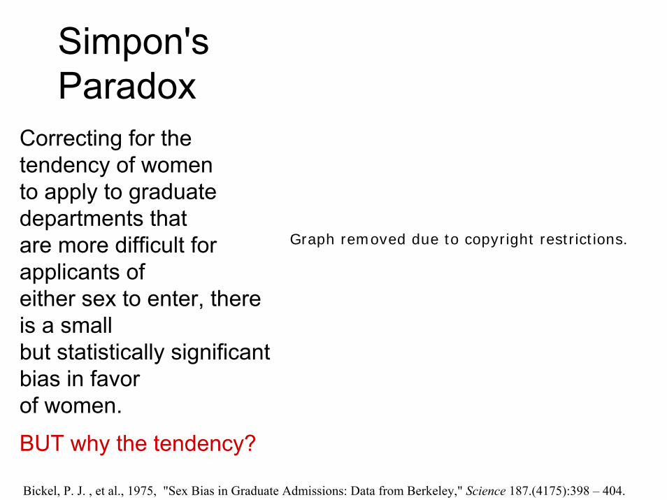
Simpon'sParadox

Bickel, P. J. , et al., 1975, "Sex Bias in Graduate Admissions: Data from Berkeley," Science 187.(4175):398 – 404.

Correcting for the tendency of womento apply to graduate departments thatare more difficult for applicants ofeither sex to enter, there is a smallbut statistically significant bias in favorof women.

BUT why the tendency?

Graph removed due to copyright restrictions.

Type-III error

• "At issue here is the importance of good descriptive and exploratory statistics rather than mechanical hypothesis testing with yes-no answers...The attempt to give an "optimal" answer to the wrong question has been called "Type-III error". The statistician John Tukey (e.g., 1969) argued for a change in perspective..."Gigerenzer, G., 2004,“Mindless Statistics,” J. of Socio-Economics 33:587-606.

Problem Set #5

1. Parameter estimationMake a probability plotMake an estimate by regressionMake an MLE estimateEstimate yet another wayComment on "goodness of fit"

2. Hypothesis testingFind a journal paper using the "null ritual"Suggest improvements (validity, insight, communication)

Next Steps• Between now and next Monday

– Read Tufte "Visual and Statistical Thinking: Displays of Evidence for Making Decisions"

• Friday, 6 April– Recitation to support PS#5

• Monday, 9 April– Session on descriptive statistics and graphics– PS#5 due, NO NEW HW ASSIGNED

• Wednesday, 11 April– Session on Regression (no pre-read)

• Friday, 13 April– Session to support the term project– Be prepared to stand up and talk for 5 minutes about your

ideas and your progress

A proposal to the NSF Design of Experiments …s Null Hypothesis Testing 1. Set up a statistical...

Documents

Transcript of A proposal to the NSF Design of Experiments …s Null Hypothesis Testing 1. Set up a statistical...