NQAA Technical Memorandum NMFS
87
NQAA Technical Memorandum NMFS SEPTEMBER 1993 REPORT OF THE TWO AERIAL SURVEYS FOR MARINE MAMMALS IN CALIFORNIA COASTAL WATERS UTILIZING A NOAA DeHAVlbLANB TWIN OTTER AIRCRAFT MARCH 9-APRIL 7,-l991 AND FEBRUARY 8-APRIL 6,1992 James V. Carretta Karin A. Forney NOAA-TM-N MFS-S W FSC-185 U.S. DEPARTMENT OF COMMERCE National Oceanic and Atmospheric Administration National Marine Fisheries Service Southwest Fisheries Science Center
Transcript of NQAA Technical Memorandum NMFS

NQAA Technical Memorandum NMFS
SEPTEMBER 1993
REPORT OF THE TWO AERIAL SURVEYS
FOR MARINE MAMMALS IN CALIFORNIA
COASTAL WATERS UTILIZING A
NOAA DeHAVlbLANB TWIN OTTER AIRCRAFT
MARCH 9-APRIL 7,-l991 AND FEBRUARY 8-APRIL 6,1992
James V. Carretta Karin A. Forney
NOAA-TM-N MFS-S W FSC-185
U.S. DEPARTMENT OF COMMERCE National Oceanic and Atmospheric Administration National Marine Fisheries Service Southwest Fisheries Science Center

NQAA Technical Memorandum NMFS
The National Oceanic and Atmospheric Administration (NOM), organized in 1970, has evolved into an agency which establishes national policies and manages and conserves our oceanic, coastal, and atmospheric resources. An organizational element within NOM, the Office of Fisheries is responsible for fisheries policy and the direction of the National Marine Fisheries Service (NMFS).
In addition to its formal publications, the NMFS uses the N O M Technical Memorandum series to issue informal scientific and technical publications when complete formal review and editorial processing are not appropriate or feasible. Documents within this series, however, reflect sound professional work and may be referenced in the formal scientific and technical literature. i

NOAA Technical Memorandum NMFS This TM series IS used for documentation and timely communicailon of preliminary results interim reports or special purpose information, and have not received complete formal review, editorial control. or deiahd editing
SEPTEMBER 1993
REPORT OF THE TWO AERIAL SURVEYS
FOR MARINE MAMMALS IN CALIFORNIA
COASTAL WATERS UTILIZING A
NOAA DeHAVlLLAND TWIN OTTER AIRCRAFT
MARCH 9-APRIL 7,1991 AND FEBRUARY 8-APRIL 6,1992
James V. Carretta Karin A. Forney
L.a Jolla Laboratory, SWFSC National Marine Fisheries Service, NOAA
P.O. Box 271 La Jolla, California 92038-0271
NOAA-TM-N M FS-SW FSC- 1 85
U.S. DEPARTMENT OF COMMERCE Ronald H. Brown, Secretary National Oceanic and Atmospheric Administration D. James Baker, Under Secretary for Oceans and Atmosphere National Marine Fisheries Service Nancy Foster, Acting Assistant Administrator for Fisheries

CONTENTS
List of Tables ......................................... List of Figures ........................................ IntrQduction ........................................... Survey objectives ...................................... Materials and Methods ..................................
Study Area ........................................ Scientific Personnel .............................. Equipment .......................................... Duty Stations ..................................... Data Collection Procedures ........................
Results ................................................ Discussion ............................................. S ~ a r y ................................................ Acknowledgements ....................................... Literature Cited ....................................... Tables ................................................. Figures ................................................ Appendix ...............................................
i
Page
ii
iv
1
2
2
6
7
10
13
13
16
35
7 0

LIST OF TABLES Page
Table 1.
Table 2.
Table 3A.
Table 3B.
Table 4.
Table 5.
Table 6.
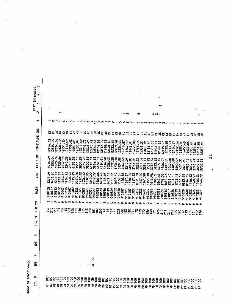
Flowchart of species codes used during 1991-1992 aerial surveys for marine mammals. Generic species codes are also shown................... ....... 16 Species sighted during 1991-1992 aerial surveys. The number of on and off-effort sightings for each species are shown in parentheses ................. 17 All cetacean and pinniped sightings (including off- effort sightings) made during 1991 aerial survey. Sightings are listed alphabetically by species code. Species present in the school are listed with their percent composition of the school to the
- right of each species. The sighting number and type, (P) primary, (S ) secondary, or (0) off effort, are given for each sighting. The observer who made the sighting is also given. School size estimates represent the llbestll estimate from individual observers................................. ............ 18 All cetacean and pinniped sightings (including off- effort sightings) made during 1992 aerial survey. Sightings are listed alphabetically by species code. Species present in the school are listed with their percent composition of the school to the right of each species. The sighting number and type, (P) primary, (S) secondary, or (0) off effort, are given for each sighting. The observer who made the sighting is also given. School size estimates represent the llbesttl estimate from individual observers.... ......................................... 25
Number and percent of kilometers surveyed, sightings, sightings/100 km, total # animals seen, mean group size, and animals/100 km, stratified by Beaufort sea state for 1991-1992 aerial surveys. Data include on- effort cetacean sightings made by primary and secondaryobservers ................................... 31
Individual number of sightings, kilometers surveyed, and rates of detecting cetacean schools, stratified by Beaufort sea state, for all observers during 1991- 1992 aerial surveys. Only on-effort cetacean sighting data are shown. Sightings made by both primary and secondary observers are included. ..................... 32
Sighting rates and number of kilometers searched by primary and secondary observers, stratified by percent
ii

Table 7.
glare and Beaufort sea state for 1991-1992 aerial surveys. The number of kilometers searched for each category are shown in parentheses. Glare values were recorded to the nearest 5%. * Kilometer total (38,754) is three times the actual number of transect miles surveyed (12,918), because glare is scored seperately for each of the three observers .......................33
Sighting rates and number of kilometers searched by primary and secondary observers, stratified by percent cloud cover and Beaufort sea state for 1991-1992 aerial surveys. The number of kilometers searched for each category are shown in parentheses. Cloud cover values were recorded to the nearest 5%. The number o f kilometers surveyed for each of the three observerrs are equal for each cloud category, because cloud cover is scored once for all three observers searchingsimultaneously .............................. 34
iii

Figure 1.
Figure 2.
Figure 3.
Figure 4 .
Figure 5.
Figure 6.
Figure 7.
Figure 8.
Figure 9.
Figure 10.
Figure 11.
Figure 12.
Figure 13.
Figure 14.
LIST OF FIGURES Page
Study area with two overlapping transect grids. The solid lines represent Grid 1, the dotted lines Grid 2. .....................,.................. 35 Completed transects (solid lines) for 1991, and - a posteriori geographic strata (separated by dotted lines) used in analysis by Forney and Barlow (1993) .......................*............... 36
Completed transects (solid lines) for 1992, and - a posteriori geographic strata (separated by dotted lines) used in analysis by Forney and Barlow (19931.. ..................................... 37
All marine mammal sightings made during 1991 survey. On and off-effort sightings are included...38
All marine mammal sightings made during 1992 survey. On and off-effort sightings are included...39
All marine mammal sightings made during 1991-1992 surveys. On and off-effort sightings are included. Square symbols represent 1991 sightings; plus signs 1992 sightings ...................................... 40
Common dolphin sightings during 1991 and 1992 aerial surveys for marine mammals...................41
Risso's dolphin sightings during 1991 and 1992 aerial surveys for marine mammals...................42
Pilot whale sightings during 1991 and 1992 aerial surveys for marine mammals...... .................... 43
Northern right whale dolphin sightings during 1991 and 1992 aerial surveys for marine mammals..........44
Pacific white-sided dolphin sightings during 1991 and 1992 aerial surveys for marine mammals..........45
Killer whale sightings during 1991,and 1992 aerial surveys for marine mammals,......... ................ 46 Dall's porpoise sightings during 1991 and 1992 aerial surveys for marine mammals...................47
Harbor porpoise sightings during 1991 and 1992 aerial surveys for marine mammals...................48
iv

Figure 15.
Figure 16.
Figure 17.
Figure 18.
Figure 19.
Figure 20.
Figure 21.
Figure 22.
Figure 23.
Figure 24.
Figure 25.
Figure 26.
Figure 27.
Figure 28.
Figure 29.
Figure 30.
Figure 31.
Figure 32.
Figure 33.
Bottlenose dolphin sightings during 1991 and 1992 aerial surveys for marine mammals .,.................49
Cuvier'a beaked whale sightings during 1991 and 1992 aerial surveys for marine mammals .............. 50 Unidentified ziphiid sightings during 1991 and 1992 aerial surveys for marine mammals ................... 51 Unidentified Mesoplodon beaked whale sightings during 1991 and 1992 aerial surveys for marine mammals .............................................52
Minke wh,ale sightings during 1991 and 1992 aerial surveys for marine mammals .......................... 53
Blue whale sightings during 1991 and 1992 aerial surveys for marine mammals .......................... 54
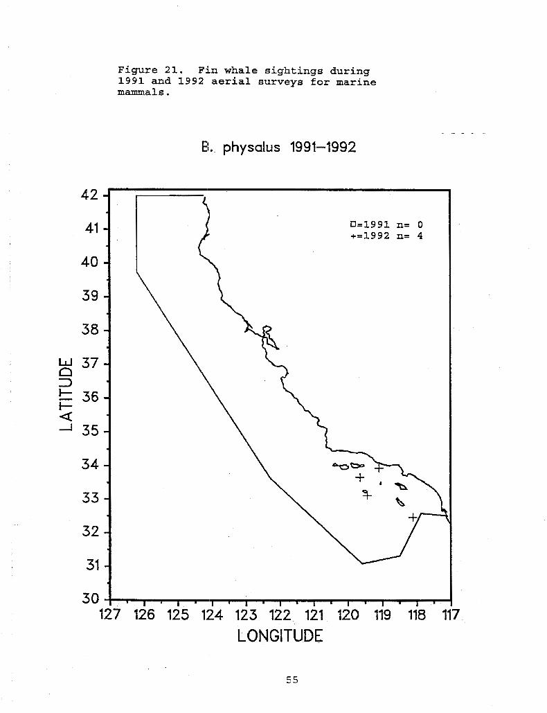
Fin whale sightings during 1991 and 1992 aerial surveys for marine rnammals..,................;...7...55
Gray whale sightings during 1991 and 1992 aerial surveys for marine mammals..........................56
Humpback whale sightings during 1991 and 1992 aerial surveys for marine mammals .................. 57 Right whale sightings during 1991 and 1992 aerial surveys for marine mammals..........................58
Sperm whale sightings during 1991 and 1992 aerial surveys for marine mazmals..........................59
California sea lion sightings during 1991 and 1992 aerial surveys for marine mammals...................60
Harbor seal sightings during 1991 and 1992 aerial surveys for marine mammals...................,.......61
Northern elephant seal sightings during 1991 and 1992 aerial surveys for marine mammals..............62
Northern fur seal sightings during 1991 and 1992 aerial surveys for marine mammals...................63
Sea otter sightings during 1991 and 1992 aerial surveys :for marine mammals...........................64
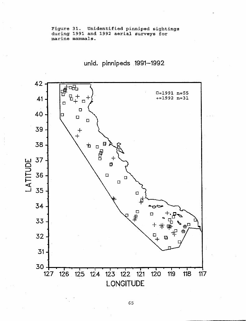
Unidentified pinniped sightings during 1991 and 1992 aerial surveys for marine manunals..........65
Unidentified dolphin sightings during 1991 and 1992 aerial surveys for marine mammals. ............. 66 Unidentified whale sightings during 1991 and 1992 aerial surveys for marine mammals...................67
V

Figure 34.
Figure 35.
.<
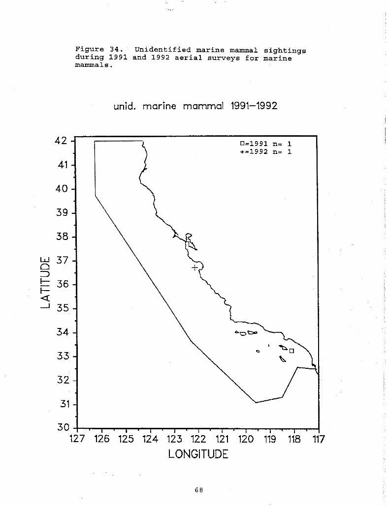
Unidentified marine mammal sightings during 1991 and 1992 aerial surveys for marine mammals..... ..... 68 Leatherback turtle sightings during 1991 and 1992 aerial surveys for marine mammals...................69
. .
vi

REPORT OF TWO AERIAL SURVEYS FOR MARINE MANMALS IN CALIFORNIA COASTAL WATERS UTILIZING A NO= DEHAVILLAND TWIN OTTER AIRCRAFT
MARCH 9, 1991 - APRIL 7, 1991 AND FEBRUARY 8, 1992 - APRIL 6, 1992
James V. Carretta and
Karin A. Forney
INTRODUCTION
This report presents the preliminary results of two aerial surveys conducted for marine mammals in the waters off the coast of California during 1991 and 1992. The objective of the surveys was to obtain winter abundance estimates for cetacean species commonly found in coastal California waters. The aerial surveys were designed to seasonally complement a ship-based survey conducted during the summer/fall of 1991 (Hill and Barlow 1992). The two aerial surveys were conducted in winter/spring, when average sea surface temperatures in California waters are coldest, whereas the ship survey was conducted during the warmest season. Estimates of abundance with statistical confidence limits for the 1991 aerial survey are presented in Forney and Barlow (1993). Summer abundance estimates for cetaceans in California waters based on a ship survey are presented in Barlow (1993). Estimates of abundance for pinnipeds were not calculated from the aerial survey data. These populations are monitored by ground counts or aerial photogrammetry counts at their breeding colonies (Lowry and Perryman 1992). However, sighting information for pinnipeds encountered during the two aerial surveys is included in this report.
Motivation for the study results from the incidental take of cetaceans in drift and set gillnets along the California coast, and the need to determine the impact of this mortality upon cetacean populations. For most of the common cetacean species in California waters, estimates of abundance were at least ten years old, and without statistical confidence limits (Dohl et al. 1980, 1983). Estimates of abundance with statistical confidence limits were available for common dolphins (Delphinus delphis); however, these estimates were based on survey data collected in the mid-1970’s (Dohl et al. 1986). In order to determine the impact of gillnet fisheries on cetacean populations, current estimates of abundance for each species were needed.
The California gillnet fishery is divided into t w o main types, each targeting different species. Barlow et al. (in press) briefly review the two fishery types. In the drift gillnet fishery, shark and swordfish are the target species. Drift gillnets are used in offshore waters from the Mexican border to the Oregon border, and are usually fished 20 to 200 miles from the coast. The set gillnet fishery utilizes bottom gillnets and trammel nets to target halibut
1

and angel shark. This fishery operates from the Mexican border north to about Bodega Bay. Set gillnets are fished in shallow water, usually less than 50 fathoms. Marine mammal species that have become entangled in gillnets or have shown evidence of entanglement include common dolphin (Delphinus delphis), Pacific white-sided dolphin (Laqenorhvnchus oblicnridens), bottlenose dolphin (Tursiops truncatus), northern right whale dolphin (Lissodelphis borealis), Risso's dolphin (Grampus crriseus), Dall's porpoise (Phocoenoides dalli), harbor porpoise (Phocoena phocoena), short-finned pilot whale (Globicephala macrorhvnchus), minke whale (Balaenoptera acutorostrata), gray whale (Eschrichtius robustus), Cuvier's beaked whale (Ziphius cavirostris), mesoplodont beaked whales (Mesoplodon spp.), sperm whale (Physeter macrocephalus), California sea lion (Zalophus californianus) , harbor seal (Phoca vitulina), and elephant seal (Mirounsa ancrustirostris).
Survey Objectives
1. The primary objective of the aerial surveys was to obtain winter abundance estimates for the common cetacean species in California waters. The surveys were also designed to seasonally complement a ship-based survey that was completed in sununer/fall 1991 (Hill and Barlow 1992).
2. To establish a baseline for detecting seasonal and interannual changes in marine mammal abundance.
3. To collect distributional information on cetacean species in California waters.
4. To utilize photogrammetric techniques on common dolphins (Delphinus delphis) and other delphinid species to determine length and stock identity.
MATERIALS AND METHODS
Study Area
The study area (Figure 1) extends beyond the continental shelf edge of the California coast, to roughly the 3000-4000m depth contour. It was selected to encompass all of the known drift-net fishing area, based on effort data for California Department of Fish and Game (CDFG) blocks. In Central/Northern California (CNC) , this extends from the coast to approximately 100 nmi perpendicular distance offshore. In the Southern California Bisht (SCB), the study area is bounded by the U.S. / Mexico border in the south and extends out to approximately 150 nmi offshore (the edge of the CDFG blocks). It then follows a straight line northwestward to a point 100 nmi off of Pt. Conception, connecting with the CNC area. The transect lines were chosen without reference to oceanographic features or bottom
2

topography. Generally, surveys were flown in a northeast or northwest direction to minimize glare, unless glare was eliminated by high cloud cover.
A total of 154 transects formed two approximately uniform, overlapping grids with lines spaced roughly 45-50 nmi apart and formed an overall grid with lines spaced approximately 22-25 nmi apart (Figure 1). The second grid was shifted from the first by 1/2 of a grid unit. Initially, the first grid was surveyed to provide coarse coverage of the entire California coast. Once this grid was nearly completed, the transects forming the second grid were flown to provide finer-scale coverage of the study area.
Scientific Personnel
1991 Survey
Dr. Jay Barlow -NMFS/SWFSC James Carretta -NMFS/SWFSC Karin Forney *-NMFS/SWFSC
Susan Kruse -NMFS/SWFSC Carrie LeDuc -NMFS/SWFSC Richard LeDuc -NMFS/SWFSC
Pilots
Lt. Tim O'Mara -NOAA/AOC Lt. Julie Vance -NOAA/AOC LCDR Pat Wehling --NOAA/AOC LCDR Mike White --NOAA/AOC
-- 1992 Survey
Dr. Jay Barlow -NMFS/SWFSC James Carretta -NMFS/SWFSC Darlene Everhart -.NMFS/SWFSC Karin Forney -NMFS/SWFSC Susan Kruse -NMFS/SWFSC Carrie LeDuc -NMFS/SWFSC Mary Lycan -NMFS/SWFSC
Pilots
Principal Investigator/Observer Marine Mammal Observer Principal Investigator & Survey- Marine Marine Marine
CoordinatoE/Observer Mammal Observer Mammal Observer Mammal Observer
Principal Investigator/Observer Survey Coordinator/Observer Marine Mammal Observer Principal Investigator/Observer Marine Mammal Observer Marine Mammal Observer Marine Mammal Observer
Lt . Tim 0' Mara -,NOAA/AOC Lt. Steve Nokutis-NOAA/AOC LCDR Mike White -NOAA/AOC
Abbreviations: NOAA - National Oceanic and Atmospheric Administration
AOC - Aircraft Operations Center (Miami) NMFS - National Marine Fisheries Service SWFSC- Southwest Fisheries Science Center
All marine mammal observers had prior experience with identifying marine mammals in the field, either from ship-board
3
I
platforms, aerial platforms, or both. In addition, intensive training on species identification and group size estimation for aerial survey work was provided to all 'observers before the start of each survey.
Equipment
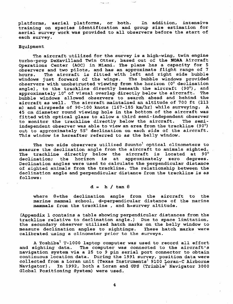
The aircraft utilized for the survey is a high-wing, twin engine turbo-prop DeHavilland Twin Otter, based out of the NOM Aircraft Operations Center (AOC) in Miami. The plane has a capacity for 5 observers and two pilots, and has an approximate flight range of 7 hours. The aircraft is fitted with left and right side bubble windows just forward of the wings. The bubble windows provided observers with unobstructed viewing from the horizon (0' declination angle), to the trackline directly beneath the aircraft (go ' ) , and approximately 10' of visual overlap directly below the aircraft. The bubble windows allowed observers to search ahead and behind the aircraft as well. The aircraft maintained an altitude of 700 ft (213 m) and airspeeds of 90-100 knots (167-185 km/hr) while surveying. A 45 cm diameter round viewing hole in the bottom of the aircraft was fittedwith optical glass to allow a third semi-independent observer to monitor the trackline directly below the aircraft. The semi- independent observer was able to view an area from the trackline (90') out to approximately 55' declination on each side of the aircraft. This window is hereafter referred to as the belly window.
The two side observers utilized Suunto' optical clinometers to measure the declination angle from the aircraft to animals sighted. The trackline directly below the aircraft is located at 90' declination; the horizon is at approximately zero degrees. Declination angles were used to calculate the perpendicular distance of sighted animals from the trackline. The relationship between the declination angle and perpendicular distance from the trackline is as follows:
d = h / t a n 8
where 8=the declination angle from the aircraft to the marine mammal school, &perpendicular distance of the marine mammals from the trackline , and h=survey altitude.
(Appendix 1 contains a table showing perpendicular distances from the trackline relative to declination angle.) Due to space limitation, the secondary observer utilized hatch marks on the belly window to measure declination angles to sightings. These hatch marks were calibrated using a clinometer prior to the surveys.
A Toshiba' T-1000 laptop computer was used to record all effort and sighting data. The computer was connected to the aircraft's navigation system via a 25 to 9 pin serial port connector to obtain continuous location data. During the 1991 survey, position data were collected from a Loran unit (Texas Instruments' 9100 Loran-C Airborne Navigator). In 1992, both a Loran and GPS (Trimble' Navigator 3000 Global Positioning System) were used.
4

An event-driven, Pascal program was used to record effort and sighting data. The program automatically obtained current position data every minute, and, again when any survey events were recorded. These events included changes in altitude, airspeed, environmental conditions, observer positions, and sighting information. During a sighting, the program provided dynamic distance and bearing information to assist in the relocation of animals.
Aerial photogrammetry was used to obtain length data for cetaceans, and to distinguish stock differences in delphinids, specifically common dolphins (Delphinus delphis) . Aerial photogrammetry was also used to verify species identifications. A 127 nun format, KA-45 military reconnaissance camera was mounted in the belly window of the plane. The camera mount was moveable so that it could be positioned away from the window during survey effort, to prevent obscuring the belly observer's view of the trackline. The camera has a 152 mn focal length lens, and a forward motion compensator to eliminate blurring by forward aircraft motion. Photographs were taken with Kodak' 3404 Plus-X black and white film, which was exposed through a Wratten 9 filter to increase contrast between subject and water. A second Toshiba' T-1000 laptop computer was linked to the aircraft's radar altimeter to obtain accurate and continuous altitude data during photographic operations. Photogrammetric methods are reviewed in Perryman and Lynn (1993).
A Realistic' voice-activated cassette recorder was linked to the aircraft headsets to record all conversation while surveying. The recorded conversationalt data documented all survey activity during the flights, but was only used as a backup to computer-recorded data.
Fluorescein dye markers were dropped from a PVC plastic chute located behind the plane's cockpit whenever a sighting was made. The dye markers were used as an aid in relocating marine mammals after an initial sighting was -de.
Duty Stations
The aerial survey team consisted of five observers and two pilots. Five observers rotated through 4 duty stations and one rest position every 30 to 45 minutes. The four duty stations were: left bubble window, right bubble window, data recorder, and belly window observer. The left and right bubble windows were designated as "primary observer" stations, and the belly window observer was designated as a Ilsecondary observer. I' The following is a description of the duty stations.
'-Reference to trade names does not imply endorsement by the NMFS.
5
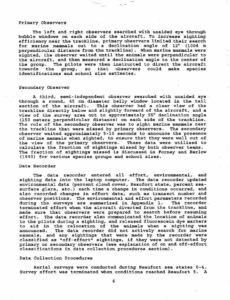
Primary Observers
The left and right observers searched with unaided eye through bubble windows on each side of the aircraft. To increase sighting efficiency near the trackline, primary observers limited their search for marine mammals out to a declination angle of 12’ (1004 m perpendicular distance from the trackline). When marine mammals were sighted, the observer waited until the animals were perpendicular to the aircraft, and then measured a declination angle to the center of the group. The pilots were then instructed to direct the aircraft towards the group, so that observers could make species identifications and school size estimates.
Secondary Observer
A third, semi-independent observer searched with unaided eye through a round, 45 cm diameter belly window located in the tail section of the aircraft. This observer had a clear view of the trackline directly below and slightly forward of the aircraft, and a view of the survey area out to approximately 55’ declination angle (150 meters perpendicular distance) on each side of the trackline. The role of the secondary observer was to sight marine mammals near the trackline that were missed by primary observers. The secondary observer waited approximately 5-10 seconds to announce the presence of marine mammals when sighted, to ensure that they were well out of the view of the primary observers. These data were utilized to calculate the fraction of sightings missed by both observer teams. The fraction of sightings missed is discussed in Forney and Barlow (1993) for various species groups and school sizes.
Data Recorder
The data recorder entered all effort, environmental, and sighting data into the laptop computer. The data recorder updated environmental data (percent cloud cover, Beaufort state, percent sea- surface glare, etc.) each time a change in conditions occurred, and also recorded changes in effort data, such as transect number and observer positions. The environmental and effort parameters recorded during the surveys are summarized in Appendix 1. The recorder terminated effort when the aircraft diverted from the trackline, and made sure that observers were prepared to search before resuming effort. The data recorder also communicated the location of animals to the pilots during a sighting, and released fluorescein dye markers to aid in the relocation of the animals when a sighting was announced. The data recorder did not actively search for marine mammals, and any sightings that were made by the recorder were classified as “off-effort. sightings, if they were not detected by primary or secondary observers (see explanation of on and off-effort classifications in data collection procedures section).
Data Collection Procedures
Aerial surveys were conducted during Beaufort sea states 0-4. Survey effort was terminated when conditions reached Beaufort 5. A
6

summary of Beaufort scale conditions is given in Appendix 1.
Sightings were recorded as either I1on-efforti1 or lloff-effortii. llOn-effortfl sightings were those made by primary and secondary observers while the aircraft was flying along a predetermined transect line, and all three observers were actively searching for marine mammals. Sightings were categorized as Itoff-effortt1 in the following four cases: 1. Sightings made while the three observers were not actively searching along the transect line (i.e. when in transit) 2. Sightings made by the pilot, the recorder, or the resting observer, but missed by the primary and secondary observers. 3. Additional sightings made while circling to re-locate an on-effort sighting. 4. Sightings made beyond 12' declination angle (1004 m perpendicular distance). When a sighting was made, the observer who made the sighting announced the presence of marine mammals. The data recorder then released a fluorescein dye marker from the aircraft, terminated survey effort, and entered the sighting information into the laptop computer. The aircraft then circled back to the location of the marine mammals. The data entry procedures used during the survey are summarized .in Appendix 1.
During the sighting, the aircraft typically made several passes over the group of animals. Observers made species identifications at this time, and took notes on the features they observed. After a consensus was reached on the identification of the species present, the aircraft circled widely around the sighting area so that observers could obtain school size estimates. Observers made three estimates, a best, high, and low estimate of the number of animals thought to be present. The observers entered their estimates into personal notebooks without discussing them, to avoid biasing or influencing each other. These estimates were entered into the data files at the end of the day by the survey coordinator.
Occasionally, it was not possible to identify marine mammals to species. In these instances, the animals were assigned a higher taxonomic identification (i . e. "unidentified dolphint1 or "unidentified whale") if a positive identification could not be made. In some cases, the observer could narrow the identification down to one of two species, for example, Ilcommon dolphin" or "Pacific white- sided dolphin". In this case, the codes for both species were combined: (DDLO) . The species codes utilized during both surveys are summarized in Table 1.
RESULTS
A total of 433 on-effort sightings were recorded during the two surveys in Beaufort sea states 0 through 4, accounting for a total of 19,410 animals, comprising 18 cetacean species, 4 pinniped species, one mustelid species, and one sea turtle species. Of these 433 sightings, 213 were cetacean sightings, totalling 19,061 animals. Of the 213 on-effort cetacean sightings, 177 were made by primary observers, and 36 by the secondary observer. A total of 40 off- effort sightings were recorded during the two surveys. Six species of cetaceans were photographed with the large format military reconnaissance camera mounted in the aircraft. Aerial photographs of
7

"" ---
Grampus qriseus, Delphinus delphis, Laqenorhvnchus oblimidens, and Lissodelphis borealis will be analyzed by the SWFSC photogrammetry group along with additional photographs obtained during 1993 aerial surveys in progress. Length determinations will be used to clarify geographical stock identities of these species (Perryman and Lynn 1993). In addition to the above species, aerial photographs of Phvseter macrocephalus and a single north Pacific right whale Eubalaena qlacialis (Carretta and Lynn, in press) were obtained.
Although the 1992 survey occurred over a two-month period, and the 1991 survey was restricted to one month, the number of kilometers surveyed was greater in 1991 than 1992 due to poorer weather conditions in 1992. 7036 kilometers were flown in 1991, and 5882 km were flown in 1992. The distribution of survey coverage is shown in Figures 2-3, for 1991 and 1992, respectively. In 1991, survey coverage was concentrated in the inner SCB, and north of Cape Mendocino (40.5'N latitude), where two passes of the survey grid were completed. Between Pt. Conception and Cape Mendocino in 1991 survey coverage was fairly uniform, although some gaps in effort occurred west of Pt. Arena (39'N), and Pt. Conception. One pass of the survey grid was completed in this area. In 1992, most survey effort was concentrated south of Pt. Conception, with two passes of the survey grid completed in the most near-shore waters. Large gaps in effort occurred between San Francisco Bay north to Cape Mendocino in 1992. High winds and low fog caused gaps in survey coverage during both surveys, especially between 37'N and 40.5'N latitude. One pass of the survey grid was completed north of Cape Mendocino in 1992. Good survey coverage in the SCB for both surveys was a result of this area
n close proximity to the base of operation (San Diego) and ely better weather conditions.
Table 2 lists the species sighted during both survey years, with the number of on-effort sightings in parentheses. The locations of all sightings (on and off effort) for all species are plotted in Figures 4-35. Tables 3A and 3B summarize sighting information for all on and off-effort sightings for all species encountered, including unidentified sightings, for 1991 and 1992, respectively. All sighting rates presented in this report refer to on-effort cetacean sightings only.
A total of 12,918 km were surveyed in Beaufort sea state conditions 0-4. Most survey effort was conducted during Beaufort 3 conditions (5740 km, 44.4% of all effort). In general, sighting rates declined with increasing Beaufort. The highest rate (2.35 sightings/100 km), occurred during Beaufort 2 conditions, and the lowest rate (1.14 sightings/100 km), during Beaufort 4 conditions. The average sighting rate for both years combined was 1.65 sightings/100 km. The sighting rate for the 1991 survey (1.81 sightings/100 km), was greater than the sighting rate for the 1992 survey (1.46 sightings/100 km), but the number of animals seen per 100 km was virtually the same for the two years (147.0 and 148.2, respectively). The mean group size for animals sighted (cetaceans only) was similar for both years (1991 = 73.8 animals/sighting, 1992 = 88.9 animals/sighting). The number of sightings, total number of animals seen, mean group size, kilometers surveyed, sightings/100 km,
8

and animals/100 km, stratified by Beaufort sea state for both years, are summarized in Table 4.
The number of kilometers searched by each of the 8 observers varied from 2305 to 7914 km. Observer sighting rates varied from 0.27 to 0.87 sightings/100 km. Individual sighting rates varied relative to Beaufort, but data pooled for all 8 observers shows that sighting rates decreased with increasing Beaufort. Sighting rates pooled across 8 observers ranged from a high of 0.78 sightings/100 km in Beaufort 2, to a low of 0.38 sightings/100 km in Beaufort 4. The average sighting rate for individual observers for both years combined was 0.55 sigbtings/100 km. The number of sightings made, number of kilometers searched, and the rates of detecting cetacean schools for each of the 8 observers stratified by Beaufort, are summarized in Table 5. Numeric codes for observers have been used rather than initials in Table 5 to provide anonymity of individual results.
The effect of sea-surface glare and cloud cover on sighting rates was examined. Tlnree glare and cloud categories were chosen to represent poor, fair, and good searching conditions across the three categories. The categories were divided so that each had a similar amount of effort. The effects of sea-surface glare and cloud cover were examined f o r primary and secondary observers separately.
Sea-Surface Glare
Primary observer sighting rates decreased with increasing sea- surf ace glare. The highest sighting rates (0.96 and 0.99 sightings/100 km) occurred in glare conditions of 0-35%, for right and left observers, respectively. Sighting rates decreased to 0.77 and 0.48 sightings/100 km in glare conditions of 40-65%' and 0.59 and 0.48 sightings/100 km in glare conditions of 70-loo%, for right and left observers, respectively. For the secondary observer, sighting rates were highest in the poorest glare conditions. The secondary observer sighting rate for the 70-100% glare category was 0.39 sightings/100 km. This sighting rate was nearly double the rates found for glare Conditions of 0-35% (0.24/100 km), and 40-65% (0.21/100 km). Table 6 summarizes the sighting rates and number of kilometers searched by primary and secondary observers, stratified by percent sea-surface glare and Beaufort sea state.
Cloud Cover
For primary observers, the lowest sighting rates were recorded during overcast conditions (cloud cover 65-100%). The rate of detecting cetacean schools in this category was 1.11 sightings/100 km. Sighting rates were highest in cloud cover of 15-60% (1.48/100 km), and similar in cloud cover of 0-10% (1.47/100 km). Secondary observer sighting rates were higher with increasing cloud cover. The highest rate (0.33/100 km) occurred in cloud cover of 65-loo%, and the lowest rate (0.25/'100 km) in cloud cover of 0-10%. Table 7 summarizes the sighting rates and number of kilometers searched for primary and secondary observers, stratified by percent cloud cover and Beaufort sea state. Cloud cover was not analyzed separately for
9

right and left observers because cloud cover was scored once for all three observers searching simultaneously (see Appendix 1).
DISCUSS ION
We compared the seasonal distribution of the most commonly sighted cetacean species during winter/spring 1991-1992 aerial surveys with those sighted during a summer/fall ship survey conducted in 1991 (Hill and Barlow 19921, and compared any observed seasonal differences with prior findings for each species. We also discuss the observed effects of cloud and glare on sighting rates.
Species Accounts
Dall's porpoise (Phocoenoides dalli) were the most commonly sighted cetacean (n=38) during the 1991-1992 aerial surveys, although the average group size for these sightings was only 3 animals. During the winter/spring aerial surveys, Dall's porpoise were distributed uniformly within the survey area, from the Channel Islands north to the California/Qregon border (Figure 13). Hill and Barlow (1992) reported 128 sightings of Dall's porpoise during a summer/fall ship survey. All sightings of Dall's porpoise during that study occurred north of Pt. Conception (34.5' N latitude), with no sightings being made near the Channel Islands. Doh1 (1980) notes that Dall's porpoise is infrequently seen in the SCB during warm- water periods, and Leatherwood et al. (1972) state that during periods of cold-water intrusion, Dall's porpoise may be seen as far south as Bahia de Ballenas, Baja California, Mexico. Our seasonal findings seem to agree with prior data indicating a tendency of Dall's porpoise to avoid warm-water masses.
Northern right whale dolphins (Lissodelphis borealis) were sighted 31 times during 1991-1992 aerial surveys. Most of the sightings occurred over shelf waters in the inner SCB, near the Channel Islands, although sightings were recorded as far north as the California/Qregon border (Figure 10). Hill and Barlow (1992) did not record any Lissodelphis sightings in the inner SCB during the summer/fall, when shelf waters are warmer. All of their Lissodelphis sightings that occurred south of Pt. Conception were well west of the Channel Islands, approximately 100 nmi or more from shore. Lissodelphis also occurred north to Pt. Arena (39.5' N latitude), California during that study. Leatherwood and Walker (1979) and Doh1 et al. (1980) reported that Lissodelphis was a seasonal visitor to the SCB, increasing in abundance during cool water (winter) periods, and declining in abundance during the summer/fall when water temperatures increased. Comparison of winter/spring aerial survey data with summer/fall ship survey data supports these prior findings .
Common dolphins (Delphinus delphis) were sighted 27 times during the two aerial surveys. All but two of these sightings occurred south of Pt. Conception (Figure 7). Hill and Barlow (1992) reported 182 sightings of Delphinus from a ship survey conducted in the summer/fall of 1991. They divided common dolphin sightings into short and long-beaked forms. Genetic and morphological evidence
10

indicates that these two forms may represent different species (Heyning and Perrin 1991, Rose1 1992). The two forms are not distinguishable from an aircraft, although the use of aerial photogrammetry may be used to separate the two (Perryman and Lynn 1993). Delphinus sightings (short-beaked form) during the 1991 ship survey were distributed from the SCB north and westward to approximately 130' W longitude and 39' N latitude. The long-beaked form was found primarily south of Pt. Conception, with a cluster of sightings recorded near the islands of Santa Cruz, Santa Rosa, and San Miguel. The major difference in the distribution of common dolphin (within 100-150 nmi of the coast) between the two surveys is that they were primarily found south of Pt. Conception in winter/spring, and dislpersed north and west with increasing water temperatures in the summer/fall. It should be noted that Barlow (1993) shows the distribution of common dolphin extending to the edge of his study area, approximately 300 nmi offshore, and north to 39.5' N latitude, while the 1991-1992 aerial survey study area only extended 100-150 nmi from shore. This complicates the detection of seasonal movements for this species. However, the apparent seasonal change in distribution (within 100-150 nmi of the coast) is in general agreement with the work of Dohl (1986), who found that Delphinus were more widely distributed in the SCB during warm water periods. Dohl also found that the abundance of Delphinus in the SCB increased seasonally, during warm-water periods. However, surveys conducted in 1991 (Forney and Barlow 1993, Barlow 1993) covering both the cold-water and warm-water periods respectively, showed that the abundance of common dolphins were very similar for the two oceanographic periods.
Gray whales (Eschrichtius robustus) were sighted 25 times during the two aerial surveys. Most sightings occurred near the coast or around the northern Channel Islands, with sightings being recorded as far north as Cape Mendocino (40.5' N latitude), California. The summer/fall 1991 ship survey recorded only two sightings, one near Pt. Reyes, the other near the California/Oregon border (42' N). The 1991 ship survey was conducted when most gray whales have already migrated north through California waters.
Pacific white-sided dolphins (Lasenorhynchus oblisuidens) were sighted 21 times during aerial surveys. They were seen in the SCB, from 32' N latitude, north to approximately 41.5' N latitude. Approximately half of the sightings were recorded south of Pt. Conception (Figure 11). Hill and Barlow (1992) reported 18 sightings of white-sided dolphin,, which were distributed from Pt. Conception north to Pt. Arena. Moist sightings were found within 150 nmi of the coast in both surveys. Comparison of the distribution of white-sided dolphin between the two surveys shows that an apparent south to north shift occurred between the winter/spring and surrrmer/fall periods. Leatherwood et al. (1984) stated that there may be evidence of seasonal fluctuation o f Lasenorhynchus off of southern California, during November through April, when peak abundances were recorded. Dohl et al. (1980) found that Laqenorhynchus moved inshore and to the southern extreme of the SCB as waters cooled seasonally. Comparison of Lasenorhynchus distributions between the winter/spring aerial and summer/fall ship surveys support past findings that show
11

Lasenorhvnchus moving north of the SCB during warm water periods.
Rissols dolphins (Grampus sriseus) were sighted 20 times during the aerial surveys, and 32 times during the ship survey. During the aerial surveys, Grampus was found primarily around the Channel Islands in the SCB, and north within 30 nmi of the coast to about Pt. Reyes (Figure 8). Ship survey results also found Grampus abundant in the SCB, with additional sightings well offshore (200 nmi and beyond) and north to about Cape Mendocino. Both surveys showed similar distributions for this species within 150 nmi of the mainland. No apparent north/south or inshore/offshore shift in distribution was detected between the two surveys. This contrasts with Dohl et al. (1980), who found that Grampus increased in numbers and moved inshore with an increase in water temperature in the SCB. During periods of cooling, Grampus were found to move offshore and south in the SCB (Dohl et al. 1980).
Of special interest was a sighting of a rare north Pacific right whale (Eubalaena slacialis) , which was sighted on 24 March 1992, southwest of San Clemente Island California (Figure 24). This whale was photographed with a large format military reconnaissance camera mounted in the belly window of the aircraft. This whale represented only the 12th reliable record of this species from California waters since the year 1900 (Carretta and Lynn, in press). Recent population estimates for right whales in the northeast Pacific range from Ita few individuals" (Klinowska 1991), to the low hundreds (Berzin and Doroshenko 1982, Braham and Rice 1984).
Cloud and Glare Effects
The observed increase in secondary observer sighting rates with increasing glare and cloud conditions may be an artifact of the survey design. The secondary observer only announced sightings that were missed by the primary observers. It is apparent that higher glare and cloud conditions caused the primary observers to miss more sightings, which would, in turn, make more sightings llavailable" to the secondary observer. Barlow et al. (1988) and Forney et al. (1991) have shown that apparent densities of harbor porpoise significantly decreased with an increase in cloud cover. Sea-surface glare (from sun glare or due to clouds) may not have been as much of a handicap in detecting marine mammals for the secondary observer as for the primary observers, otherwise, one would expect a decline in sighting rates for the secondary observer with increasing cloud and glare levels. The secondary observer generally had a better view of the sea surface from the trackline out to 150 meters perpendicular distance than the primary observer. One reason for this is that the secondary observer always had a line of sight perpendicular to the sea surface, which reduces the apparent amount of glare relative to that experienced by the primary observers.
We have presented cetacean and pinniped sighting data for two years of aerial surveys in California coastal waters. Overall
12

sighting rates (primary and secondary observers pooled) for cetaceans decreased with increasing Beaufort. Sighting rates were variable among individual observers. Sighting rates for primary observers declined with increasing glare and cloud levels. Sighting rates for the secondary observer increased with an increase in cloud and glare levels. Seasonal distributions of the most commonly sighted cetacean species in California waters appears to have south/north and inshore/offshore components, which coincided with cold and warm water periods, respectively.
ACKNOWLEDGEMENTS
The success and completion of the two surveys was the result of the excellent work and cooperation of all those involved. We would like to give special thanks to NOAA pilots Steve Nokutis, Tim O'Mara, Pat Wehling, Mike White, and Julie Vance for their expertise, patience and professionalism during the surveys. The data collected were the result of many dedicated observers spending long days aboard the aircraft, in often less than perfect weather conditions. We would like to thank Jay Barlow, Darlene Everhart, Sue Kruse, Carrie LeDuc, Richard LeDuc, and Mary Lycan for their time and the high quality data that were collected. Jay Barlow and Jim Cubbage wrote the survey program that made for less labor-intensive data collection procedures during both surveys. Wayne Perryman and Morgan Lynn provided a large format camera and technical assistance for photographing cetacean species during the surveys. Carrie LeDuc obtained many aerial photographs of cetaceans with this system. We thank Steve Leatherwood for providing the training for observers. This work was done und.er marine mammal permit #748 issued to the Southwest Fisheries Science Center, and permits GFNMS-01-92 and CINMS-01-92 issued by the Gulf of the Farallons and Channel Islands National Marine Sanctuaries, respectively. Funding for the surveys was provided by the NMFS Office of Protected Resources, Washington D.C. The manuscript was improved by the suggestions of Jay Barlow, Terry Farley, Fred Julian, Carrie LeDuc, and Richard LeDuc.
LITERATURE CITED
Barlow, J., R. Baird, J. Heyning, IC. Wynne, A. Manville, L. Lowry, D. Hanan, J. Sease, and V. Burkanov. (in press). A review of cetacean and pinniped mortality in coastal fisheries along the west coast of the U . S . and Canada and the east coast of the U.S.S.R. Report of the International Whaling Commission, Special Issue:
Barlow, J. 1993. The abundance of cetaceans in California waters estimated from ship surveys in summer/fall 1991. NOAA, National Marine Fisheries Service, Southwest Fisheries Science Center Administrative Report LJ-93-09. 39pp.
Barlow, J., C.W. Oliver, T.D. Jackson, and B.L. Taylor. 1988. Harbor porpoise, phoceena Dhocoena, abundance estimation for California, Oregon, and Washington: 11. Aerial surveys. Fishery Bulletin 86(3):433-444.
13

Berzin, A.A. and N.V. Doroshenko. 1982. Distribution and abundance of right whales in the North Pacific. Report of the International Whaling Commission 32:381-383.
Braham, H.W. and D.W. Rice. 1984. The Right Whale, Balaena glacialis. Marine Fisheries Review 46(4):38-44.
Carretta. J.V., and M.S. Lynn. (in press) Right whale (Eubalaena slacialis) sighting off San Clemente Island, California. Marine Mammal Science.
Dohl, T.P., K.S. Norris, R.C. Guess, J.D. Bryant and M.W. Honig. 1980. Cetacea of the Southern California Bight. Part 11, Summary of marine mammal and seabird surveys of the Southern California Bight area, 1975-1978. Final Report to the Bureau of Land Management, NTIS Rep. No. PB81248189. 414 pp.
Dohl, T.P., R.C. Guess, M.L. Duman, and R.C. Helm. 1983. Cetaceans of central and northern California, 1980-1983: Status, abundance and distribution. OCS Study MMS 84-0045. Minerals and Management Service contract #14-12-0001-29090. 284pp.
Dohl, T.P., M.L. Bonnell, and R.G. Ford. 1986. Distribution and abundance of common dolphin (Delphinus delphis) , in the southern California Bight: A quantitative assessment based upon aerial transect data. Fishery Bulletin 84:333-343.
Forney, K.A., D.A. Hanan, and J. Barlow. 1991. Detecting trends in harbor porpoise abundance from aerial surveys using analysis of covariance. Fishery Bulletin 89:367-377.
Forney, K.A. and J. Barlow. 1993. Preliminary winter abundance estimates for cetaceans along the California coast based on a 1991 aerial survey. Rep. Int. Whal. Cornmn. (in press).
Heyning, J.E. and W.F. Perrin. 1991. Re-examination of two forms of common dolphins (genus Delphinus) from the eastern North Pacific; evidence for two species. NOAA, National Marine Fisheries Service, Southwest Fisheries Science Center Administrative Report LJ-91-28, Southwest Fisheries Science Center, La Jolla, CA. 53 pp.
Hill, P.S. and J. Barlow. 1992. Report of a marine mama1 survey of the California coast aboard the research vessel McArthur July 28-November 5, 1991. NOAA-TM-NMFS-SWFSC-169, 103pp.
Klinowska, M. 1991. Northern Right Whale. In: Dolphins, Porpoises, and Whales of the World: The IUCN Red Data Book. IUCN, Gland, Switzerland, and Cambridge, U.K. pp. 351-357.
Leatherwood, J.S., W.E. Evans and D.W. Rice. 1972. The whales, dolphins, and porpoises of the eastern North Pacific. Naval Undersea Center, San Diego, Calif. NUC TP 282.
I
Leatherwood, S., and W.A. Walker. 1979. The northern right whale
14

dolphin Lissodelr3his borealis Peale in the eastern North Pacific. In Win:n, H.E., and B.L. Olla (eds.), Behavior of Marine Mammals, p. 85-141. Plenum Press, New York-London.
Leatherwood, S., R.R. Reeves, A.E. Bowles, E.S. Stewart and K.R. Goodrich. 1984 e Distribution, seasonal movements, and abundance of Pacific white-sided dolphins in the eastern north Pacific. Sci. Reg. Whales Res. Inst. 35:129-157.
Lowry, M.S. and W.L. Perryman. 1992. Aerial photographic census of California sea lion (Zalophus californianus) pups at San Miguel Island, California for 1987-1990, and San Nicolas Island, California for 1990. Administrative Report LJ-92-19, 19pp.
Perryman, W.L. and M.S. Lynn. 1993. Identification of geographic forms of common dolphins (Delphinus delphis) from aerial photogrammetry. Marine Mammal Science 9(2):119-137.
Rosel, P.E. 1992. Genetic population structure and systematic relationships of some small cetaceans inferred from mitochondrial DNA sequence variation. Ph.D. thesis presented to the University of California, San Diego. 191pp.
15

-,
Table 1. Flovchart of species codes used during 1991-1992 aerial surveys for marine nramnals. Generic species codes are also shown.
Phocoena phocoena
Phocoenoides
Lagenorhynchus ob1 iquidens
Delphinus delphis
Stenella coeruleoalba
Lissodelphis borealis
Tursiops truncatus
Grampus griseus
Pseudorca crassidens
Globicehala macrorhvnchus
Orcinus orca --
Mesoplodon spp.
Zihius cavirostris
Berardius bairdii
spp.
Balaenoptera acutorostrata
B. edeni
B. borealis
- 8. physalus
- - - -
E. musculus
Megaptera novaeangliae
Eschrfchtius robustus
Eubalaena glacialis
Physeter macrocephalus
PP
PD
LO
DD
sc
LB
11
GG
PC
Gn
00
UM
21
BD
UK
BA
BE
BP
BM
MN
ER
EG
U D r Unid. porpoise
'Whitebelly' dolphin
Small delphinid
Unid. delphinid
Large delphinid
Small whale
Small ziphiid
Unid. ziphiid
uw' Unid. whale
Fin/sei/Bryde's whale
Unid. large baleen whale
Unid. large whale
AT
cu
Zatophus californianus
Ewetopias jubatus
Arctocephalus townsendii
Caltorhinus ursinus
-- MA pv I kS Phoca vitulina
Mirounga angustirostris
-0T
Unid. sea lion
Unid. sea lion/fur seal
Unid. fur seal
-PU Unid. pinniped
Unid. seal
OTHER CODES USED: EL Enhydra lutris Sea otter MM unidentified marine m a w 1 DC Dermochelys coriacea Leatherback turtle UT unidentified turtte
16
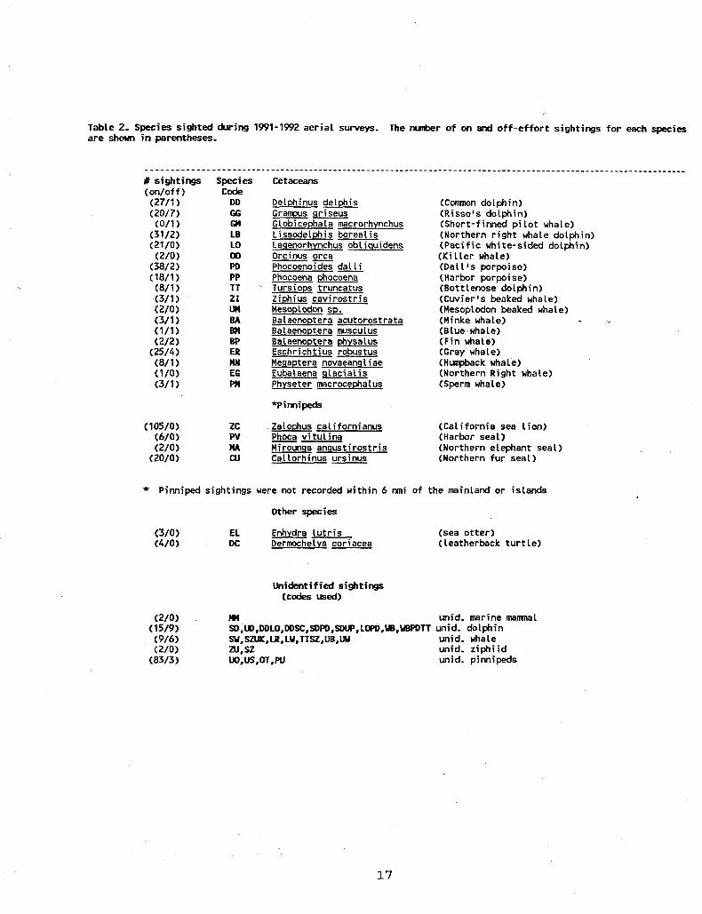
Table 2. species sighted during 1991-1942 aerial surveys. The nunber of on and off-effort sightings for each specis are s h m in parentheses.
. - - - - - - - - - - - -___-__________________ Cetaceans
Delphinus delphis G r a m s griseus Globicephala macrorhynchus Lissodelphis borealis Lagenorhvnchus oblisuidens Orcinus orca Phocoenoides Phocoena phocoena Tursiops truncatus Ziphius cavirostris Mesoplodon Balaenoptera acutorostrata Balaenoptera rmsculus Balaenoptera phvsalus Esch r i ch t i us robus tus Megaptera novaeamliae Eubalaena glacialis Phvseter macrocephalus
*Pimi@
--
( C m n dolphin) (Risso's dolphin) (Short-finned pilot whale) (Northern right whale dolphin) (Pacific white-sided dolphin) (Killer whale) (Dallis porpoise) (Harbor porpoise) (Bottlenose dolphin) (Cwier's beaked whale) (Mesoplodon beaked whale) (Minke whale) (Blue whale) (Fin whale) (Gray whale) (Hunpback whale) (Northern Right whale) (Sperm whale)
( 105/0) ZC ZaloDhus californianus (California sea lion)
(20/0) cu Callorhinus ursinus (Northern fur seal)
W O ) PV -- Phoca vitulina (Harbor seal) (2/0) n.4 Mirwnga angustirostris (Northern elephant seal)
* Pinniped sightings were not recorded within 6 mi of the mainland or islands
Other species
(3/0) EL Enhvdra lutris (sea otter) ( 4 / 0 ) DC Dermochelvs coriacea (leatherback turtle)
Unidentified sightings CCOCles used)
( 2/0 ) m unid. marine mamnal (15/9) SD,U),DO,LO,DOSC,SDPD,SWP,tOPD,~,YBPDTT mid. dolphin ( 916 ) SU,SZUK,LR,LU,TTSZ,UB,UU unid. whale (2/0) m,sz unid. tiphiid
(83/3) w,us,m,w unid. pinnipeds
17

..
In v) w I-
$ * - I- m W
I- v) w
M
N m
7
v)
8 W n
el z 0 -1
W
3 c I- U -I
n
I
w
I- 5
W
5 a * c #, v)
s u n v)
w
M
v) a
w
N
v) n
ap
a - v)
N In
N-N In
0 N b 0 0 L n l n M O 0
00 0 O C O 0 0 ~ 0 0 d I n N N lnN .O 0.
0 - l n N M M l n d E d u us*1 -a N
N-N b oln ln 0 ~ 0 0 0 0 0 d 0 I n 0 - lnM In 0 lnlnN00
c M
O M ~ b O r * m N N O - d a M lnu 4 ' M Nb --
c c b.3 M Z
2 NN
-N.-MN--In- - - - O l n ln In0000000NInlnM-v~-NN
V
0 N
.?d I n c o
m o 2-1
0 In
z E
N
t- I-
52" a m a-I

V h 0.
u W N 0
7
J 0 . - 0
m
M - V
W V = : s CIJ N -I
E - o. N M
- N In
In - s m n W
-I n W m m . L - I - I c I-

,-
In
2
0 000 P, P, "51k
N -
0
U pc N
0 -I
0 n
- V
V N
0 . 0 W M
3 2
m -1
m -I
P, 0.
m +
W W I-0 I-J
n n
8 k y s COP,.- - v
o w o o m o o -1 W N N J N N
0 ln
4 m
1 v)
W c a E * c v) W
c v) W
r
m c
0 e E 2
U C -
- U C
c c 4
- - L
- w
c 5
w c 4 0
n * I-
5 v)
w u n v)
w
M
v) n
w
f g O M Y
3 z 9 ) -
?i I-
-
R m 2

-

U v)
w c
IC:
c v) w c v) w
a - P
m
c
V
C LL
a
c I=
a
- u II -1
W n 2 2
?i
- -J
w
c
W I- s n *- c
z v )
x
* v ) a
w
2 v)
w
h P
I%?
- m M - N
N
N-
O 03
0 03
0 * .,
K!
s
h h
c.3 0
2 * m 2
n n
N
m 2

,' ..< .
0 0 In N
N
N
.-"
U M M N O 0 M U U 0 0 0 6s:
M 0
U 0
b c
m -1

In
* v) W + a m 2 5 . + v) W N
I- v)
W m-
cn 0
W
I3 I-
0 z
m
n
w
s w n
E I-
4
5 W
I-
w I-
d a * I-
2 v)
x
* v) n
w
M v) n
x
N
v) n
x - n v)
-- N r C
-- NN *
0 0 m o m In r C I n
0 o m o m 0 M O 0- . tM 0 0 %?to. ? *
P
m -1
R $ E n r v m m~
In- - v v
V Z v - 5 : N n n
N
0 N
0 . m '00.
o n ~n

LA
v) W t- ern
I- v) W N
I- 07 W
2
m -
W
2 c
W I-
3
U v) a
w
M a 07
N n
VI-
w "
- 0 al
m o x 2

-s
9. 0.
0 -I

m
u VI W e a m E t- VI W N
v) W m -
W c a n
n * c
c v)
0-
2 v)
w
M v) n
w
N n
P I-
m h N M -
In Ir)
N m S*
0 or N
0 m -
m m
0 U
M U
0 N U . - ,
Q O N ??? sgs! m a - __-
n u o r u l n ~ u m u m ~ m h u m ~ m m ~ ~ ~ s o u ~ u m ~ o r ~ ~ u u o r w m u o r o r h ~ a m m m
3 0 0 0 0 0 0 0 0 0 0 0 0 0 0 0 0 0 0 0 0 0 0 0 0 0 0 0 0 0 0 0 0 0 0 0 0 0 0 0 0 0 0 0
1orbb~bbororbhbbbbbbbbbbbbbbborbb~bborborororororborororor
3 O N O N N N - N O O N . - N - N N - N - ~ - N N N N O N N N N O N - - N N N - - - - - ~ Q M M M N N M M N M M N N M N N N M N N N N M N N N M M N N N M M N N M M M N M M M N M
VNNNNNNNNNNNNNNNNNNNNNNNNNNNNNNNNNNNNNNNNNNN
or- o r a
O W W U
% h N
n n n n

0 Ln N
h J
N U
N h -- .
0 N
m 2
h CO
0 A
VI
a m
O O O O O O O O O O O U O O O O O O O O O O O O O O O O M O O O O Q O O O O O O O O O O Q h O O 0000000000000000000000000000 0000000000*~00 - - - P , - - - - - - ~ r - - - - P - - - - ~ - - - - - ---------- -c
N N N N N N N N N N N N N N N N N N N N N N N N N N N N N N N N N N N N N N N N N N N

?1z?z$~?sE!!4?8rr9?kis N M C U N M N M N M N M N M M M M N N N 0000000000000000000 NNNNNNNNNNNNNNNNNNN ~ m 0 . m m m m m 0 . m P m m m m o . 0 . m m n n n n n m n n n n n n n m n n n a m
M 0.
0 m

Table 4. Number and percent of kilometers surveyed, sightings, sightings/100 km, total # animals seen, mean group size, and animals/100 km, stratified by Beaufort sea state for 1991-1992 aerial surveys. Data include on-effort cetacean sightings made by primary and secondary observers.
1991 357 1,164 3,317 2,198 (5.1%) (16.5%) (47.1%) (31.2%)
7,036 (100.0%)
1992 484 1,224 2,423 1,749 5,882 . (8.2%) (20.8%) (41.2%) (29.7%) (100.0%) ’
1991 6 38 1992 10 18
ALL 16 56
55 28 127 41 17 86 96 45 213
138.1 229.8 31.5 147.0 98.7 40.6 148.2
ALL 375.2 187.6 174.5 35.5 147.5
1991 117.1 1992 565.7 234.7
Mean group size
33.

Table 5. Individual number of sightings, kilometers surveyed, and rates of detecting cetacean schools, stratified by Beaufort sea state, for all observers during 1991-1992 aerial surveys. Only on- effort cetacean sighting data are shown. Sightings made by both primary and secondary observers are included.
01 02 03 04 05 06 07 08 ALL
4 3 0 1 1 1 1 5
16
8 2 6
18 10 2 3 7 56
12 6 8
12 24 6 9
19 96
9 4 2 12 10 0 2 6
45
33 15 16 43 45 9
15 37
213
01 02 03 04 05 06 07 08
571 393 290 447 352 206 97
171
1,351 792 517
1,604 762 595 350
1,195
3,281 1,367 1,100 3,296 2,589 1,510 1,232 2,845
2,235 1,200
398 2,567 1,448 1,054 1,122 1,818
7,439 3,752 2,305 7,914 5,151 3,364 2,801 6,028
01 02 03 04 05 06 07 08 Avg .
0.70 0.76 0.00 0.22 0.28 0.49 1.03 2.92 0.63
0.59 0.25 1.16 1.25 1.44 0.34 1.14 0.59 0.78
0.37 0.44 0.73 0.36 0.93 0.40 0.73 0.67 0.56
0.40 0.33 0.50 0.47 0.69 0.00 0.18 0.33 0.38
0.44 0.40 0.69 0.54 0.87 0.27 0.54 0.61 0.55
32

Table 6. Sighting rates and number of kilometers searched by primary and secondary observers, stratified by percent glare and Beaufort sea state for 1991-1992 aerial surveys. The mmber of kilometers searched for each category are shown in parentheses. *Kilometer total (38,754) i s three times the actuat nmber of transect miles surveyed (12,918), because glare is scored seperately for each of the three observers.
GIare values were recorded to the nearest 5%.
- - - - - - - - - - - - - - - - - . - - - - - - - - - - - - - - - - - - - - - - - - - - - - - - - - - - - - - - - - - - - - - - - - # Sightings/100 In,
(# km searched) Beaufort
loBl 2 3 4 ALL . . . . . . . . . . . . . . . . . . . . . . . . . . . . . . . . . . . . . . . . . . . . . . . . . . . . . . . . . . . . . . . . . Right observer
Glare X 0-35 0.64 1.66 0.77 0.74 0.96
40-65 0.45 1.51 0.57 0.73 0.77
(472) (1,023) (1,689) (1,081) (4,265)
(221) (731) (2,115) (1,374) (4,441)
70-100 0.67 0.47 0.77 0.40 0.59 (1149) (634) (1,937) (1,493) (4,212)
ALL 0.59 1.30 0.70 0.61 0.77 (842) (2,388) (5,740) (3,948) (12,918) ----------------------------.----~---------------*----------------
Left observer
Glare X 0-35 1.32 0.95 0.91 1.06 9-99
(379) (951) (1,214) (3777) (2,921)
40-65 0.99 0.56 0.59 0.16 0.48 (304) (720) (2,030) (1,292) (4,347)
70-100 0.63 0.98 0.56 0.22 0.48 (l!j9) (717) (2,496) (2,278) (5,650)
ALL 1..07 0.84 0.65 0.28 0.60 (842) (2,388) (5,740) (3,948) (12,918) . . . . . . . . . . . . . . . . . . . . . . . . . . . . . . . . . . . . . . . . . . . . . . . . . . . . . . . . . . . . . . . . . . .
Secondary observer
Glare 4: 0-35 0.16 0.17 0.27 0.37 0.24
(616) (1,200) (1,468) (823) (4,108)
40-65 0.00 0.14 0.27 0.18 0.21 (111) (731) (2,240) (1,666) (4,748)
70-100 0.87 0.44 0.44 0.27 0.39 (115) (457) (2,032) (1,458) (4,062)
ALL 0.24 0.21 0.33 0.25 0.28 (842) (2,388) (5,740) (3,948) (12,918) . . . . . . . . . . . . . . . . . . . . . . . . . . . . . . . . . . . . . . . . . . . . . . . . . . . . . . . . . . . . . . . . . . .
A l l observers combined
Glare X 0-35 0.til 0.88 0.64 0.66 0.71
(1,467) (3,174) (4,371) (2,281) (11,294)
40-65 0.63 0.73 0.47 0.35 0.48 (636) (2,183) (6,385) (4,332) (13,356)
70-100 0.77 0.66 0.59 0.29 0.49 (424) (1,807) (6,465) (5,2291 (13,924)
ALL 0.63 0.78 0.56 0.38 0.55 (2,528) (7,164) (17,221) (11,842) (38,754)’ . . . . . . . . . . . . . . . . . . . . . . . . . . . . . . . . . . . . . . . . . . . . . . . . . . . . . . . . . . . . . . . . . . .
33

Table 7. Sighting rates and number of kilometers searched by primary and secondary observers, stratified by percent cloud cover and Beaufort sea state for 1991-1992 aerial surveys. The number of kilometers searched for each category are shown i n parentheses. The number of kilometers surveyed for each of the three observers are equal for each cloud category, because cloud cover is scored once for at1 three observers searching simultaneously.
Cloud cover values were recorded to the nearest 5%.
________________________________________- - - - - - - - - - - - - - - - - - - - - - - - - # Sightings/100 km
(# h searched) Beaufort
081 2 3 4 ALL ________________________________________- - - - - - - - - - - - - - - - - - - - - - - - - Primary observers
Cloud % 0-10 1.25 2.43 1.26 1.02 1.47
(399) (1,483) (2,381) (1,660) (5,923)
15-60 2.91 2.21 1.67 0.67 1.48 (275) (453) (1,374) (1,199) (3,301)
65-100 0.59 1.10 1.26 0.83 1.11 (169) (453) (1,985) (1,089) (3,695)
ALL 1.66 2.14 1.36 0.86 1.37 (842) (2,388) (5,740) (3,948) (12,918)
_ _ _ _ _ _ _ _ _ _ _ * _ _ _ _ _ _ _ _ - - - - - - - - - - - - - - - - - - - - - - - - - - - - - - - - - - - - - - - - - - - - - -
Secondary observer
Cloud % 0-10 0.25 0.27 0.25 0.24 0.25
(399) (1,483) (2,381) (1,660) (5,923)
15-60 0.00 0.00 0.36 0.33 0.27 (275) (453) (1,374) (1,199) (3,301)
65-100 0.59 0.22 0.40 0.18 0.33 (169) (453) (1,985) (1,089) (3,695)
ALL 0.24 0.21 0.33 0.25 0.28 (842) (2,388) (5,740) (3,948) (12,918) ________________________________________-- - - - - - - - - - - - - - - - - - - - - - - - -
All observers combined
Cloud x 0-10 1.50 2.70 1.51 1.27 1-72
(399) (1,483) (2,381) (1,660) (5,9233)
15-60 2.91 2.21 2.04 1.01 1.76 (275) (453) (1,374) (1,199) (3,301)
65-100 1.18 1.33 1.66 1.01 1.43 (169) (453) (1,985) (1,089) (3,695)
ALL 1.90 2.35 1.69 1.12 1.65 (842) (2,388) (5,740) (3,948) (12,918) . . . . . . . . . . . . . . . . . . . . . . . . . . . . . . . . . . . . . . . . . . . . . . . . . . . . . . . . . . . . . . . . . .
34

Figure 1. Study area with two overlapping transect grids. The solid lines represent Grid 1, the dotted lines Grid 2.
41" -
40" -
39" -
38" -
37" -
36" -
35" -
34" -
33" -
32" -
31" -
Pacific 0 cea n
3 0 ° b , , , , ~, , , , , I , , , I
127" 126" 125" 124" 123" 122" 121" 120" 119" 118" 117"
Longitude
35

Figure 2. Completed transects (solid lines) for 1991 and 3 posteriori geographic strata (separated by dotted lines) used in analysis by Forney and Barlow (1993).
Pacific Ocean
1270 126" 125" 124" 123" 122" 121" 120" 119" 118" 117"
Longitude
36

Figure 3. Completed transects (solid lines) for 1992 and a Posteriori geographic strata by dotted-lines) used in analysis by Forney and Barlow (1993).
(separated
42"
41 O
40"
39"
380
37"
36'
35"
34"
33"
32"
31 "
30"
Pacific Ocean
127" 126" 125" 124" 123" 122" 121" 120" 119" 118" 117"
Longitude
37

42
41
40
39
38
37
36
35
34
33
32
31
30
Figure 4. All marine mammal sightings made during 1991 aerial survey. On and off-effort sightings are included.
All sightings 1991 n=263
127 126 125 124 123 122 121 120 119 118 117 LONGITUDE
38

Figure 5. 1992 survey. included.
All marine mammal sightings made during On and off-effort sightings are
All sightings 1992 n=210
42
41
40
39
38
w 37 Q 3 - I- 36 a A 35 f-
34
33
32
LONGITUDE
39

- -_ - - _ _ - - - _ _ are included. sightings; plus signs 1992 sightings.
iquare symbols represent i991
All sightings 91-92 n=473
42
41
40
39
38
w 37 3 k 36 I- Q --I 35
34
33
32
31
30
n
127 126 125 124 123 122 121 120 119 118 1 LONGITUDE
40
7

42
41
40
39
38
3 k 36 I- Q -I 35
34
33
32
31
30
Figure 7. and 1992 aerial surveys for marine mammals.
Common dolphin sightings during 1991
D. delphis 1991-1992
-1
0=1991 n=15 +=1992 n=13
- . - I i - 7 - ' . ' I ' l ' l B 1 '
127 126 125 124 123 122 121 120 119 118 1
LONGITUDE
41
7

Figure 8. Risso's dolphin sightings during 1991 and 1992 aerial surveys for marine mammals.
G. griseus 1991-1992
[7=1991 n=17 +=1992 n=10
W
I) I- t- Q 1
n -
127 126 125 124 123 122 121 120 119 118 117 LONGtTUDE
42

42
4'
40
39
38
37
36
35
34
33
32
31
30 I
Figure 9. and 1992 aerial surveys for marine mammals.
Pilot whale sightings during 1 9 9 1
G. inacrorhynchus 1991-1992
t
i n = 1 9 9 1 n= 0 +=1992 n= 1
- ~ ' " ' ' ' = ' ' ~ ' 1 '
127 126 125 1214 123 122 121 120 119 118 1
LONGITUDE r
43

Figure 10. Northern right whale dolphin sightings during 1991 and 1992 aerial surveys for marine mammals.
I
1
42
41
40
39
38
37
36
35
34
33
32
31
30 1
L. borealis 1991-1992
O=l99l n=24 +=1992 n= 9
1 ' l ' l = l ' l ' f ' ~ ' ~ ' f
7 126 125 124 123 122 121 120 119 118 7 LONGITUDE
44

42
41
40
39
38
37
36
35
34
33
32
31
30 1
I I ~ I ' I ' I ' I ' l ' I *
126 125 124 123 122 121 120 119 118 117
Figure 11. Pacific white-sided dolphin sightings during 1991 and 1992 aerial surveys f o r marine mannmals.
L obli qui d ens 199 1-1992
I
n=1991 +=1992
n= 8 n=13
4 5

Figure 12. Killer whale sightings during .
1991 and 1992 aerial surveys for marine mammals.
0. orca 1991-1992
42
41
40
39
38
37
36
35
34
33
32
31
30
4 6

42
41
40
39
38
w 37 n 3 k 36 t- a .-I 35
34
33
32
31
30 1
Figure 13. 1991 and 1992 aerial surveys for marine mammals.
D l a l l ' s porpoise sightings during
P. dalli 1991-1992
0=1991 n=22 +=1992 n=18
LONGITUDE
47

w 3 f- i= Q J
4 L
41
40
39
38
37
36
35
34
33
32
31
30 1
Figure 14. H a r b o r porpoise sightings during 1991 and 1992 aerial surveys for marine mammals.
P. phocoena 1991-1992
i ' t ' i . ' . , , ~ ' ~ ' ~ K 126 125 124 123 122 121 120 119 118 117
LONGfTUDE
4 8 .

42
4'
4c
39
36
34
33
32
31
30
Figure 15. Bottlenose dolphin sightings during 1991 and 1992 aerial s u r v e y s for marine mammals.
T. truncatus 1991-1992
0=1991 n= 6 +=1992 n= 3
- b ' 1 ' 1 ' 1 ' " ' " '
127 126 125 124 123 122 121 120 119 118 1'
LONGITUDE
49

42
41
40
39
38
37
36
35
34
33
32
31
30
Figure 16. Cuvier's beaked whale sightings during 1991 and 1992 aerial surveys for marine mammals.
Z. cavirostris 1991-1992
0
\
n=1991 +=1992
n= 3 n= 1
1 ' 1 m l m l n l n i , l , , ,
127 126 125 124 123 122 121 120 119 118 I' LONGITUDE
50
7

Figure 17. Unidentified ziphiid sightings during 1991 and 1992 aerial surveys f o r marine mammals.
unid. ziphiid 1991-1992
\ b
42 - I
41 - 40 - 39 - 38 - 37 -
36 - 35 - 34 -
33 - 32 -
31 - -
0=1991 n= 2 +=1992 n= 0
30 I . , , , . , , , . , , m , . , .
127 126 125 124 123 122 121 120 119 118 117
LONGITUDE
51

Figure 18. Unidentified Mesoplodon beaked whale sightings during 1991 and 1992 aerial surveys for marine mammals.
Mesoplodon sp. 1991-1992
42
41
40
39
38
37
36
35
34
33
32
31
30 1
0=1991 n= 2 +=1992 n= 0
52

42
41
40
39
38
36
-I 35 I- *
34
33
32
31
30 1
Figure 19. Minke whale sightings during 1991 and 1992 aerial, surveys far marine marmnals.
B. cicutorostrata 1991-1992
0=1991 n= 3 +=1992 n= 1
5 3

- -
A
42
41
40
39
38
37
36
35
34
33
32
31
30 1
Figure 20. Blue whale sightings during 1991 and 1992 aerial surveys for marine mammals.
B. musculus 1991-1992
I ' l ' l ' l ~ l * l . ~ s ~ i t a
7 126 125 124 123 122 121 120 119 118 1 LONGITUDE
7
54
42
41
40
39
38
36
35 I- Q
34
33
32
31
30
Figure 21. 1 9 9 1 and 1 9 9 2 aerial surveys for marine mammals.
Fin whale sighting8 during
- -
Et. physalus 1991-1992
U=1991 n= 0 +=1992 n= 4
7 LONGITUDE

. . .- ~
Figure 22. Gray whale sightings during 1991 and 1992 aerial surveys for marine mammals.
E. robustus 1991-1992
42
41
40
39
38
w 37 n 3 k 36 I-
35 a
33
32
31
3 0 ~ . , . 1 . 1 . , , 1 . 1 . 1 . 1 , 1 . 127 126 125 124 123 122 121 120 119 118 117
LONGITUDE
56
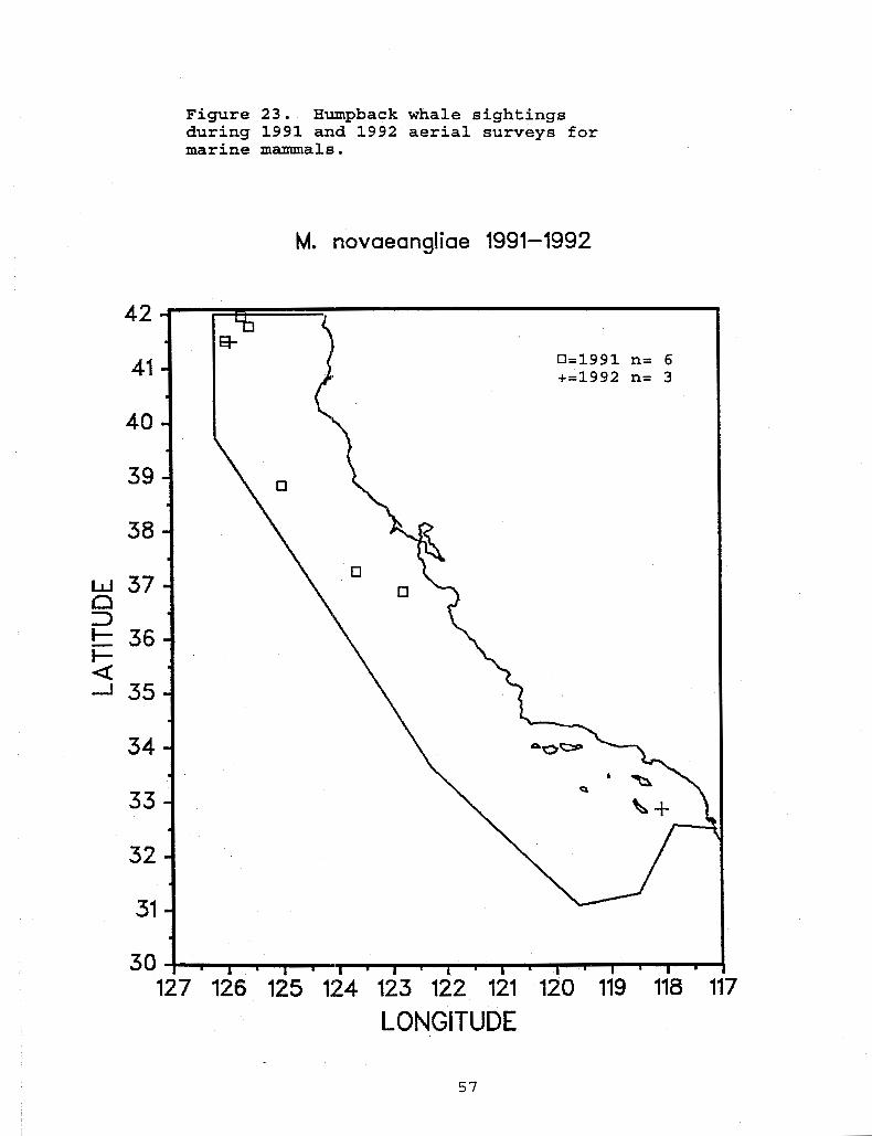
Figure 23. Humpback whale sighting8 during 1991 and 1992 aerial surveys fo r marine mammalR.
M. novaeangliae 1991-1992
57

i
Figure 24. Right whale sightings during 1991 and 1992 aerial surveys for marine mammals.
E. glacialis 1991-1992
I < 0=1991 n= 0 +=1992 n= 1
42
41
40
39
38
37
36
35
34
33
32
31
30 127 126 125 124 123 122 121 120 119 118 1
LONGITUDE
5 8

42
41
40
39
38
37
36
35
34
33
32
31
30
Figure 25. 1991 and 1992 aerial surveys f o r marine mammals.
Sperm whale sighting8 during
P, nnacrocephaius 1991-1992
n=1991 n= 1 +=1992 n= 3
127 126 125 124 123 122 121 120 is LONGITUDE
18 117
59
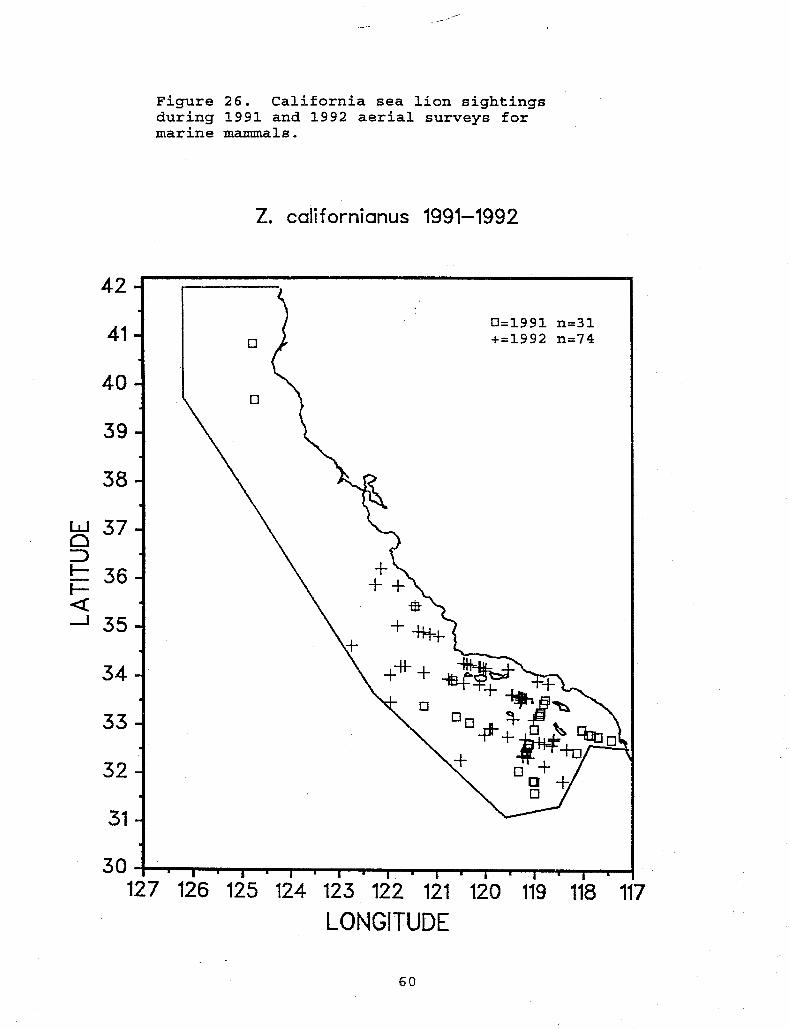
Figure 26. California sea lion sightings during 1991 and 1992 aerial surveys for marine mammals.
42
41
40
39
38
37
36
35
34
33
32
31
30
60

Figure 27. 1991 and 1992 aerial surveys for marine mammals.
Harbor seal sfghtings during
30+) ' I . l a 1 1 I I ' 127 126 125 124 123 122 121 120 119 118 117
P. vitulina 1991-1992
34 -
33 - 32 -
31 -
61

42
41
40
39
38
37
36
35
34
33
32
31
30
Figure 28. Northern elephant seal sightings during 1991 and 1992 aerial surveys for marine mammals.
1 ' 1 . 1 ' 1 . 1 . 1 . f . f . 1 '
127 126 125 124 123 122 121 120 119 118 I LONGITUDE
6 2

42
41
40
39
38
37
36
35
34
33
32
31
3 ~ , ' 1 ' l ' i ' l ' i ' i ' i ~ i ~ i ~
Figure 29. Northern fur seal sighting6 during 1991 and 1992 aerial surveys for marine mammals.
127 126 125 124 123 122 121 120 119 118 117
C. ursinus 1991-1992
i+$.\ 0=1991 n= 8
63

W
3 I- t- Q 1
n -
42
41
40
39
38
37
36
35
34
33
32
31
30
Figure 30. Sea o t t e r sighting8 during 1991 and 1992 aerial surveys for marine mammals.
sea offers 1991-1992
O=l99l +=1992
n= 3 n= 0
I ' l * i ' 1 ~ l * ~ n ~ f i ~ s 1 a
127 126 125 124 123 122 127 120 119 118 117 LONGITUDE
64
W
3 I-
n - t- J a
42
41
40
39
38
37
36
35
34
33
32
31
30 1
Figure 31. Unidentified pinniped sighting8 during 1991 and 1992 aerial surveys for marine mammals.
unid. pinnipeds 1991-1992
0=1991 n=55 +=1992 n=31
- i n I 1 ' I r n l ' i ' 1 '
7 126 125 12!4 123 122 121 120 119 118 1 7
LONGITUDE
6 5

Figure 32. Unidentified dolphin sighting8 during 1991 and 1992 aerial surveys for marine mammals.
unid. dolphins 1991-1992
42 a
41 - 40 - 39 -
38 -
37 - 36 - 35 - 34 - 33 -
32 - 31 - 30 I ' l ' & . ~ ~ ~ ~ & S ~ . , . ~ .
127 126 125 124 123 122 121 120 119 118 1 LONGITUDE
6 6
7

W c3 => I- t- 6 J
-
Figure 3 3 . Unidentified whale s igh t ings during 1 9 9 1 and 1 9 9 2 a e r i a l surveys f o r marine mammals.
mid. whales 1991-1992
42 -
41 -
40 -
39 -
38 -
37 - 36 - 35 -
34 - 33 -
32 - 31 - 30 i ' i ~ i ' l ' ~ ' ~ ' ~ ' ~ ' [ ~
127 126 125 124 123 122 121 120 119 118 1' 7 LONGITUDE
67
'-. ,
Figure 34. Unidentified marine mammal sighting8 during 1991 and 1992 aerial surveys for marine mammal8.
unid. marine mammal 1991-1992
3 0 f I I m ~ i . l . , , , , i , , , , 127 126 125 I24 123 'I22 121 120 119 118 117
LONGITUDE
68

Figure 35. Leatherback turtle sightings during 1991 and 1992 aerial. surveys for marine mammals.
Leatherback turtle 1991-1992
42
41
40
38
37 n \ 2
36
35 f- Q
34
33
32
31
30 1
69

.. .... ~
. APPENDIX 1.
DATA ENTRY
INTRODUCTION
INSTRUCTIONS FOR AERIAL STJRVEYS FOR MARINE MAMMALS
This will be the second field season of aerial surveys for marine mammals in which sighting and effort data will be recorded on a Toshiba laptop computer. Use of the laptop computer allows for increased accuracy in data collection, the capability of rapid data editing, and a quick transition time between data collection and analysis.
The data entry program (called SURVEY3) is a new and improved version of programs used on prior aerial surveys. It is an event- driven program, similar to the CRUISE program that was used on board the NOAA-ship McArthur during the 1991 CAMMS marine mama1 cruise (Hill and Barlow 1992 NOAA-TM-NMFS-SWFSC-169, 103pp.).
GENERAI; FKATURES
The basic feature of the program is that it is event-driven. You press a function key to indicate an event. Each function key has a specific assignment (eg. F2 for a sighting, F5 to toggle effort on-or-off, etc.). When you press a function key, the computer notes the time and latitude/longitude of the aircraft at the moment you pressed the key. You will not have to write down time or position (for the latter, the computer is plugged into a GPS or LORAN navigation unit). The first event you enter will be noted in the event buffer in the upper left part of the computer screen. You can continue to press other event buttons while the computer is waiting for you to respond with information on the first event. These subsequent events will stack-up in the buffer and wait for your response. There is never any rush. The time and position of the buffered events has already been recorded.
RECORDER'S RESPONSIBILITY
It is the recorder's responsibility to enter and update all sighting, effort, and weather information. Observers will verbally provide the recorder with sighting, weather, and viewing condition information while we are surveying. However, if you are the recorder, and you notice for example, a change in the Beaufort sea state, speak up and get the consensus of the observers who may have not noticed the change in Beaufort.
At times the recorder may feel overwhelmed with a lot of information all at once, especially when three observers are trying to give you weather/viewing condition information, and another observer(s) may have a sighting. In the past, observers have been good about giving the recorder the needed information in a coherent and orderly manner. The event buffer in the upper left corner of the screen stores which function keys you hit, in the order in which they were hit, and records the position and time for each. There is no need to hurry out of one event window when given other information. You can for example, (and should) hit the F2 sighting button while you are in the weather window entering data if someone has a sighting. The event-driven system, automatically records the position and time where the sighting was made, and allows you to finish entering your weather data. Once you escape out of the
7 0

weather window, the sighting window will appear, ready to receive the sighting information.
ERROR CORRECTION FEA!IXIm
Most errors that are made in entering data can be easily corrected. If you make an error that cannot be corrected immediately, or you are unsure if you entered information correctly, it is best; to document the problem using a comment statement (F10). If you make a mistake and pressed the wrong event button, you can cancel it by pressing the UNDO button (Fl). When you are entering information, into an event window, you can navigate within the window using the ENTER or arrow keys. You can continue to make changes, going from one data element to the next, until you get it perfect. If you entered a wrong value and already pressed the ESC to save it, you can go backwards to make corrections using the left and right arrow keys. These will allow you to go back in the buffer, and retrieve the event window where you want to make changes. Record a comment (FlO), concerning any changes you make. Each of the event buttons and error-recovery functions are documented in more detail below.
If you missed something or incorrectly entered data during the mayhem, use the arrow keys, which allow you to move around the event buffer, and reenter the window in which you need to fix data. You can only go back as far as the event code at the left edge of the buffer allows. If you try to go too far back in time, you will get a message that reads: WARNING - Cannot Edit earlier records. Please document correction using comments. Most corrections that you make while surveying will not require going back through that many events, but if this happens, utilize the F10 comment button to enter information. If you find yourself going back in time in the event buffer and someone has a sighting, hit the F2 SIGHT button, and then the ESC key once to get you back to real time. A sighting window will immediately appear, ready to receive information. If you did not finish editing the window that you had been in previously, you can go back to it with the arrow keys after the sighting.
SIGHTING RELOCATION FEATURES
This program has a feature that locks onto the location of the last on-effort sighting, and gives a bearing and distance back to that location once you have hit the sight button. Often, we will resight the same aniimals several times while circling to get estimates, photographs and/or identifications. Because of the movements of the anima.ls, the original sighting position is often inaccurate after several minutes of circling over the area where the animals were originally sighted. The Shift-F2 button allows you to get an updated lbearing and distance to the school each time you relocate them while circling. This makes relocation of animals progressively easier (theoretically) with each pass. Use this key to help the pilots relocate the animals after they have been sighted again after the initial sighting. Enter the current sighting number and angle where the animals were most recently seen.
MAP FEATURES
71

The SURVEY3 program also has two map features that assist in: 1. relocating lost animals, and 2. showing you graphically where you are, where you've been, and where you're going. The maps are utilized with the SHIFT-F3 keystroke. You are given two map options to choose from. The first is a map of the entire CA. coast, and study area, which shows all survey effort that has been completed to date. The second option is a local map that shows all lines flown (on or off effort) within a 1 degree square around the current position. This map is useful when you are trying to relocate a sighting. It enables you to see where the plane has circled relative to the original sighting position. This map feature was utilized by the pilots last year, and proved very effective in relocating lost sightings.
GENE- COMMANDS:
SURVEY3 Type this at the DOS prompt to start program. ESC Hit this key when done entering information in an
event window. CTRL -D Key sequence to end program.
FUNCTION KEYS:
F1 UNDO
F2 SIGHT
This key allows you to do two things. You can delete an entire event window, or undo all changes in the window since you first entered information within a window. For example, if you want to update observer position information (F61, but instead hit weather (F9), you can hit F1 to erase the undesired event window. The "W" character in the buffer symbolizing weather will be replaced by a pound (#) sign. Another use for F1 UNDO is if you want to
undo an accidental change of data in a window. For example, if you are updating values for glare, and you enter a value where there really was no change, hitting F1 will change all values in the window to
their original value.
Hit this key as soon as we are perpendicular to the animals, or when the secondary (belly) observer calls out a sighting. You will then record the following:
Observer: Observer who initially made the sighting. If more than one observer call the same sighting, whoever called sighting first is recorded.
Angle : Declination angle measured to the center of the sighted group. Sightings made to the left of the trackline are recorded as negative, those to the right are positive.
7 2

F3 BEG.TR.
F4 END TR.
F5 EFFORT
F6 OBSERVER POSITION
F7 %GLARE
Primary? : Enter Y if sighting was made by a primary (side) observer, or N if it was made by the secondary (belly)
, observer. Enter 0 if an off effort observer made the sighting.
Speciesl: Enter 2-letter code identifying species.
Species2: & If applicable, enter codes for Species3 : other sighted species in group.
Hit this key at the beginning of a new transect. Refer to the attached figures containing Transects 1-76 for Grid 1, and Transects 1 0 1 - 1 7 8 for Grid 2. The F3 key will also automatically prompt you for glare (lF7), weather (F9), altitude & speed (F8) and observer positions (Fl).
Hit this key when the transect ends. If we are immediately starting a new transect, hit F3 immediately afterwards.
This key is a toggle key that you hit whenever we begin or end effort while on a transect. Note, the large block letters in the lower left corner of the screen ithat read either OFF or ON. When the F5 key is hit, OFF will change to ON, and vice versa when struck again. This indicates whether we are on or off effort at the time. It should read ON while we are surveying. This ON/OFF message is also interactive with the begin transect (F3), and end transect (F4) keys. When you begin a transect (F3), the effort message will read ON. When you end a transect (F4), it will read OFF.
This key when hit will ask you to enter the two 1ett.er code designating observers in their
respective positions. If there is no one in the position, type off. The rear left and rear right positioins are normally unoccupied (off) . Observers initials are: (many more will be added as we go).
Jay Bar:Low JB Rick LeDuc RL Jim Carretta JC Mary Lycan ML Darlene Everhart DE Sue Rruse SK Karin Forney KF Carrie LeDuc CL
Generally, 1st and last name initials will be used, unless there is a conflict.
Ask observers for their percent glare and record them in the respective fields, to the nearest 5%. If no observer is in that position, record OFF. Glare i.s defined as percentage of viewing area obscured by sun glare, cloud glare, or even glare from wiindow reflections .
73

F8 ALTITUDE We will normally be surveying at 700 feet and 100 SPEED knots. You should verify this periodically with the
pilots.
F9 WEATHER Record weather conditions whenever they change, and at the start of a transect. They are coded as:
HazeKelp: H=haze below plane. K=kelp obscuring surface of water. N=neither haze or kelp present.
%Overcast: Record (to the nearest 5%) this as a percentage of cloud cover between the viewing area and the plane.). make this more than below!
Beaufort :
sun (i.e., on the ''sun side" of the Whoever has the best view of the sun can call. Don't give the overcast estimate a glance, otherwise you may miss animals
Water Color:
Sea smooth and mirror-like. Wind range: 0-1 knots.
Scale-like ripples, no foam crests. Wind range: 1-3 knots.
Small, short wavelets; crests have glassy appearance and do not break. Wind range: 4-6 knots.
Large wavelets; some crests begin to break; foam of glassy appearance; occasional white foam crests. Wind range: 7-10 knots.
Small waves, becoming longer; fairly frequent white foam crests. Wind range: 11-16 knots.
Moderate waves, taking a more pronounced form, many white foam crests; there may be some spray. Wind range: 17-21 knots.
L=light blue D=dark blue G=greenish blue R=red tide
The belly observer usually has the best view to evaluate water color.
F10 COMMENT Record additional comments on behavior of animals sighted, or other items of interest. Also comment when mistakes were made in the data entry, and say how they should be corrected later. Data corrections that can be done right away should be done utilizing the F1 UNDO key if possible. Try to make each line of what you type a separate comment.
74

The maximum allowable length for a single comment is two lines on the screen. If possible, keep the length of comments less than one line - this helps later when data is edited.
SHIFTED FUNCTION KEYS:,
F2 SPECIES The Shift-F2 keystroke allows you to get an updated bearing and distance to the school when you relocate the animals while circling. Enter the current sighting number and angle where the animals where most recently seen. When you escape out of this window, another window appears near the top-center of the screen that says: Last On-Eff. Sighting. It gives you the position where the animals were last seen, along with a distance and bearing back to that position.
SIGHTING
F3 MAP Use this feature to call up a map of:
1. The entire California coast with all survey effort mapped.
2. All lines flown (on or off effort) within a 1 degree area around the current position. This local map is also useful in relocating lost animals. The map shows you where we have circled in relation to where the animals were first sighted.
F4 TURTLE If a turtle is sighted, enter the two-letter observer code, declination angle, two-letter species code, and # of turtles. Also include the directiion (in clock units) in relation to the plane that the turtle was travelling. For example, if the turtle was headed to the right of the trackline, record this as a 3. Also record any associated objects: J=jellyfish, F=floating objects, R=red tide. In the comments record the approxiimate size of the turtle, whether or not a tail was visible (which would indicate that it was a male), and any other item of interest or biological significance.
F5 NEW SIGHT # The sighting numbers on the aerial survey are cumulative. The first sighting number of the day should be one greater than the last sighting number of the previous day. If for some reason, the program that keeps the sighting numbers tallied fails, the first sight number of that day would read as # 1. You can use this keystroke to update the correct sighting number for the Survey3 program.
7 5

Declination angles and perpendicular distances from the trackline
Declination angle ('1 Perpendicular distance (meters)
Southwest Fisheries Science Center, NMFS Coastal Cetacean Surveys
Key to aerial survey raw data format
Columns Entry
1-3 4 5 6-11 12 13-18 19 20-28 29
40 41-end
30-39
Line # Entry type code blank Time, format: HHMMSS blank Date, format: MMDDYY blank Latitude, format: NDD:MM.MM blank Longitude, format: WDD:MM.MM blank entered data
Kev to entry type codes:
* = position and time update (taken every minute) T = Transect start, automatically followed by V,P ,A,W. V = Viewing conditions for all 3 observer positions. Recorded as
percentage of viewing area obscured by glare. P = Observer positions (order: left front, belly, right front,
recorder).
76
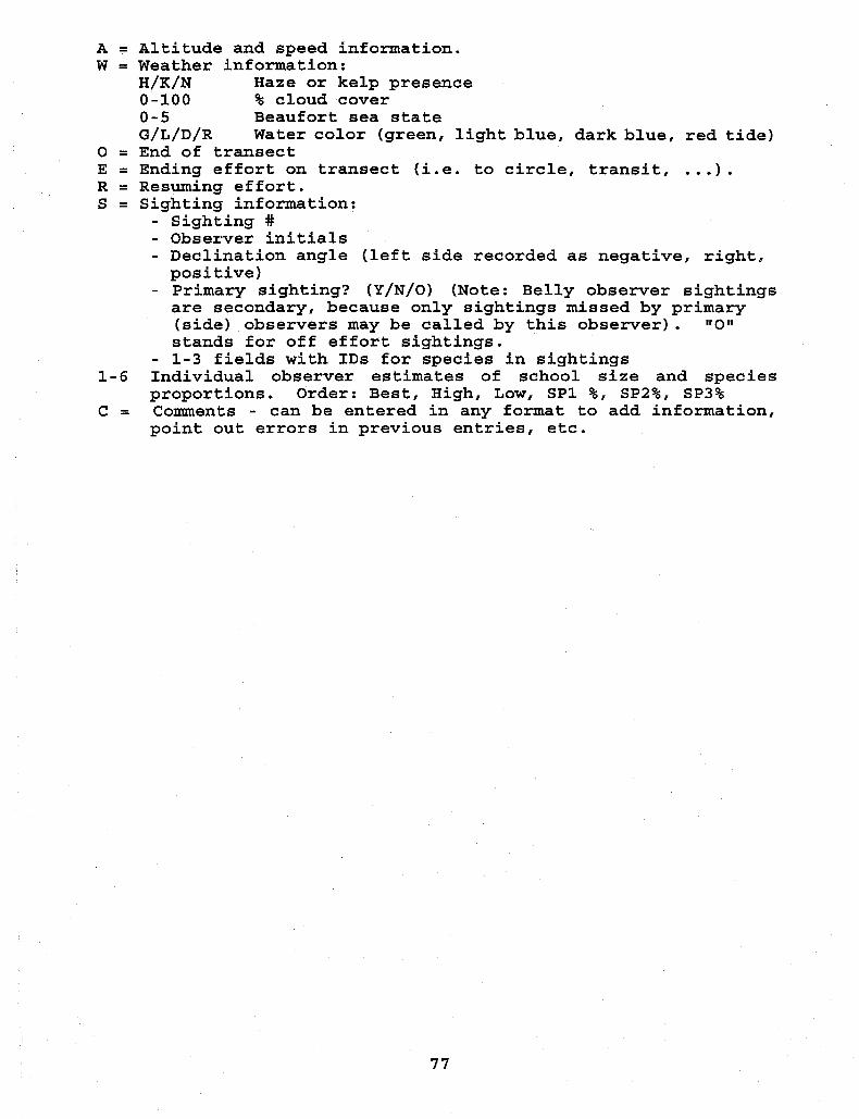
A = Altitude and speed information. W = Weather information:
H / W N Haze or kelp presence 0-100 % cloud cover 0-5 Beaufort sea state G/L/D/R Water color (green, light blue, dark blue, red tide)
0 = End of transect E = Ending effort on transect (i.e. to circle, transit, ...). R = Resuming effort. S = Sighting information:
- Sighting # - Observer initials - Declination angle (left side recorded as negative, right, positive)
- Primary sighting? (Y/N/O) (Note: Belly observer sightings are secondary, because only sightings missed by primary (side) observers may be called by this observer). 11011 stands for off effort sightings.
- 1 - 3 fields with IDS for species in sightings 1-6 Individual observer estimates of school size and species
proportions. Order: Best, High, Low, SP1 %, SP2%, SP3% C = Comments - can be entered in any format to add information,
point out errors in previous entries, etc.
77

RECENT TECHNICAL MEMORANDUMS
Copies of this and other NOAA Technical Memorandums are available from the National Technical Information Service, 5285 Port Royal Road, Springfield, VA 22167. Paper copies vary in price. Microfiche copies cost $4.50. Recent issues of NOAA Technical Memorandums from the NMFS Southwest Fisheries Science Center are listed below:
NOAA-TM-NMFS-SWFSC-175 The Hawaiian monk seal and green turtle at Pearl and Hermes Reef, 1988. B.K. CHOY and L.M. HlRUKl (November 1992)
176 Distribution of ichthyoplankton around Southeast Hancock Seamount, central North Pacific, in summer 1984 and winter 1985: data report. G.W. BOEHLERT and B.C. MUNDY (December 1992)
177 Hawaiian monk seal observations at French Frigate Shoals, 1984. J.J. ELIASON and J.R. HENDERSON (December 1992)
178 The Hawaiian monk seal at French Frigate Shoals, 1988-89. M.P. CRAIG, D.J. ALCORN, R.G. FORSYTH, T. GERRODETTE, M.A. BROWN, B.K. CHOY, L. DEAN, L.M. DENNLINGER, L.E. GILL, S.S. KEEFER, M.M. LEE, J.S. LENNOX, C.R. LORENCE, G.L. NAKAl and K.R. NIETHAMMER (December 1992)
179 The Hawaiian monk seal on Lisianski Island, 1988 and 1990. M.M. LEE, L.K. TIMME, R. VANTOORENBURG, and B.L. BECKER (March 1993)
180 Report of ecosystem studies conducted during the 1992 eastern tropical Pacific common dolphin survey on the research vessels David Starr Jordan and McArthur. V.A. PHILBRICK, P.C. FIEDLER, S.B. REILLY, R.L. PITMAN, and L.T. BALLANCE (April 1993)
181 Summary of cetacean survey data collected between the years of 1974 and 1985. T. LEE (May 1993)
182 The Hawaiian monk seal and green turtle at Pearl and Hermes Reef, 1990-1 991. M.A. FINN, J.R. HENDERSON, B.L. BECKER, and T.J. RAGEN (May 1993)
183 Summary of 1989 U.S. Tuna-Dolphin Observer Data. A.R. JACKSON (July 1993)
coastal marine mammal survey aboard the research vessel McArthur. V.A. PHILBRICK, P.C. FIEDLER and S.B. REILLY (July 1993)
184 Report of ecosystem studies conducted during the 1991 California