NOAA Technical Memorandum NMFS - SWFSC · PDF filenoaa technical memorandum nmfs april 2008 a...

NOAA Technical Memorandum NMFS

APRIL 2008

A FRAMEWORK FOR ASSESSING THE VIABILITY OF

THREATENED AND ENDANGERED SALMON AND STEELHEAD IN

THE NORTH-CENTRAL CALIFORNIA COAST RECOVERY DOMAIN

Brian C. Spence Eric P. Bjorkstedt

John Carlos Garza Jerry J. Smith

David G. Hankin David Fuller

Weldon E. Jones Richard Macedo

Thomas H. Williams Ethan Mora

NOAA-TM-NMFS-SWFSC-423

U.S. DEPARTMENT OF COMMERCE National Oceanic and Atmospheric Administration National Marine Fisheries Service Southwest Fisheries Science Center

NOAA Technical Memorandum NMFS

The National Oceanic and Atmospheric Administration (NOAA), organized in 1970, has evolved into an agency that establishes national policies and manages and conserves our oceanic, coastal, and atmospheric resources. An organizational element within NOAA, the Office of Fisheries is responsible for fisheries policy and the direction of the National Marine Fisheries Service (NMFS).

In addition to its formal publications, the NMFS uses the NOAA Technical Memorandum series to issue informal scientific and technical publications when complete formal review and editorial processing are not appropriate or feasible. Documents within this series, however, reflect sound professional work and may be referenced in the formal scientific and technical literature.

NOAA Technical Memorandum NMFS This TM series is used for documentation and timely communication of preliminary results, interim reports, or special purpose information. The TMs have not received complete formal review, editorial control, or detailed editing.

APRIL 2008

A FRAMEWORK FOR ASSESSING THE VIABILITY OF

THREATENED AND ENDANGERED SALMON AND STEELHEAD IN

THE NORTH-CENTRAL CALIFORNIA COAST RECOVERY DOMAIN

B. C. Spence1, E. P. Bjorkstedt1,3, J. C. Garza1, J. J. Smith2, D. G. Hankin3, D. Fuller4, W. E. Jones5, R. Macedo6, T. H. Williams1, E. Mora1

1 NOAA National Marine Fisheries Service Southwest Fisheries Science Center

110 Shaffer Road, Santa Cruz, CA 95060

2 Department of Biological Sciences, San Jose State University

3 Department of Fisheries Biology, Humboldt State University

4 Bureau of Land Management, Arcata Field Office

5 California Department of Fish and Game (retired), Ukiah

6 California Department of Fish and Game, Northern Region

NOAA-TM-NMFS-SWFSC-423

U.S. DEPARTMENT OF COMMERCE Carlos M. Gutierrez, Secretary

National Oceanic and Atmospheric Administration Vice Admiral Conrad C. Lautenbacher, Jr., Under Secretary for Oceans and Atmosphere

National Marine Fisheries Service James W. Balsiger, Acting Assistant Administrator for Fisheries

i

Table of Contents

List of Figures..................................................................................................................................iii

List of Tables ................................................................................................................................... iv

List of Plates .....................................................................................................................................v

Acronyms and Abbreviations ...........................................................................................................vi

Acknowledgements ..........................................................................................................................vi

Executive Summary ........................................................................................................................vii

1 Introduction..................................................................................................................................1

1.1 Background .............................................................................................................................1

1.2 Relationship Between Biological Viability Criteria and Delisting Criteria ....................................5

1.3 Population Delineations and Biological Viability Criteria .........................................................10

1.4 Report Organization ...............................................................................................................12

2 Population Viability Criteria.......................................................................................................13

2.1 Key Characteristics of Viable Populations ...............................................................................13

2.2 Population-Level Criteria ........................................................................................................16

Extinction Risk Based on Population Viability Analysis (PVA).....................................................20

Effective Population Size/Total Population Size Criteria .............................................................22

Population Decline Criteria ......................................................................................................26

Catastrophe, Rate and Effect Criteria ........................................................................................29

Spawner Density Criteria..........................................................................................................33

Hatchery Criteria .....................................................................................................................44

Summary of Population Metrics and Estimators .........................................................................48

Critical Considerations for Implementation................................................................................51

3 ESU Viability Criteria.................................................................................................................53

3.1 Characteristics of Viable ESUs ...............................................................................................53

3.2 ESU-level Criteria ..................................................................................................................54

Representation Criteria.............................................................................................................55

Redundancy and Connectivity Criteria .......................................................................................57

3.3 Example Scenarios of Application of ESU-Viability Criteria .....................................................60

4 Assessment of Current Viability of Salmon and Steelhead Populations within the NCCC

Recovery Domain......................................................................................................................67

4.1 Central California Coast Coho Salmon ....................................................................................68

Population Viability ..................................................................................................................68

ESU Viability ...........................................................................................................................75

ii

4.2 California Coastal Chinook Salmon.........................................................................................76


ESU Viability ...........................................................................................................................82

4.3 Northern California Steelhead.................................................................................................83


ESU Viability ...........................................................................................................................91

4.4 Central California Coast Steelhead..........................................................................................91


ESU Viability ...........................................................................................................................97

4.5 Conclusions ...........................................................................................................................97

References..................................................................................................................................... 100

Appendix A. Revisions to NCCC Population Structure Report.................................................... 116

Appendix B. Discussion of Density Criteria and their Application............................................... 145

Appendix C. Guidance for Evaluating Hatchery Risks ................................................................ 163

iii

List of Figures

Figure 1. Approximate historical geographic boundaries of ESA-listed salmon and steelhead ESUs and DPSs in the North-Central California Coast Recovery Domain. ...............................................3

Figure 2. Hypothetical fluctuations in the abundance for a healthy population showing no long-term trend in abundance (A) versus a population undergoing a long-term decline (B)....................28

Figure 3. Hypothetical example where an order of magnitude decline in abundance occurs over a single year (A) versus three years (B).........................................................................................31

Figure 4. Hypothetical example catastrophic decline in abundance, showing three possible trajectories: A) apparent trend toward recovery from the decline, B) relatively stable abundance following the decline, and C) continued downward trend in abundance........................32

Figure 5. Relationship between risk and spawner density as a function of total habitat potential for coho salmon, Chinook salmon, and steelhead.. ...........................................................................37

Figure 6. Historical population structure of a hypothetical diversity stratum within an ESU..................61

iv

List of Tables

Table 1. Criteria for assessing the level of risk of extinction for populations of Pacific salmonids. Overall risk is determined by the highest risk score for any category............................................ 18

Table 2. Description of variables used to describe population size in the population viability criteria. ....................................................................................................................................19

Table 3. Current salmon and steelhead hatchery programs operating within the NCCC Recovery Domain, their purpose, mode of operation, and status..................................................................49

Table 4. Estimation methods and data requirements for population viability metrics .............................50

Table 5. Historical structure, current conditions, and potential recovery planning scenarios for a hypothetical diversity stratum in a listed ESU (illustrated in Figure 6) ..........................................62

Table 6. Projected population abundances (Na) of CCC-Coho Salmon independent populations corresponding to a high-risk (depensation) thresholds of 1 spawner/IPkm and low-risk (spatial structure/diversity=SSD) thresholds based on application of spawner density criteria (see Figure 5). .................................................................................................................................69

Table 7. Current viability of CCC-Coho Salmon independent populations based on metrics outlined in Tables 1 and 4. .....................................................................................................................71

Table 8. Projected population abundances (Na) of CC-Chinook Salmon independent populations corresponding to a high-risk (depensation) threshold of 1 spawner/IPkm and low-risk (spatial structure/diversity=SSD) thresholds based on application of spawner density criteria (see Figure 5) ..................................................................................................................................79

Table 9. Current viability of CC-Chinook salmon independent populations based on metrics outlined in Tables 1 and 4 .........................................................................................................81

Table 10. Projected population abundances (Na) of NC-Steelhead independent populations corresponding to a high-risk (depensation) threshold of 1 spawner/IPkm and low-risk (spatial structure/diversity=SSD) thresholds based on application of spawner density criteria (see Figure 5) ..................................................................................................................................84

Table 11. Current viability of NC-steelhead independent populations based on metrics outlined in Tables 1 and 4..........................................................................................................................87

Table 12. Projected population abundances (Na) of CCC-Steelhead independent populations corresponding to a high-risk (depensation) threshold of 1 spawner/IPkm and low-risk (spatial structure/diversity=SSD) thresholds based on application of spawner density criteria (see Figure 5) ..................................................................................................................................92

Table 13. Current viability of CCC-steelhead independent populations based on metrics outlined in Tables 1 and 4.. ........................................................................................................................95

v

List of Plates

Plate A1. Diversity strata for populations of Central California Coast coho salmon ............................ 139

Plate A2. Diversity strata for populations of fall-run California Coastal Chinook salmon.................... 140

Plate A3. Diversity strata for populations of spring-run California Coastal Chinook salmon ............... 141

Plate A4. Diversity strata for populations of winter-run Northern California steelhead........................ 142

Plate A5. Diversity strata for populations of summer-run Northern California steelhead..................... 143

Plate A6. Diversity strata for populations of Central California Coast steelhead................................. 144

vi

Acronyms and Abbreviations

CC-Chinook salmon California Coastal Chinook salmon Evolutionarily Significant Unit

CCC-coho salmon Central California Coast coho salmon Evolutionarily Significant Unit

CCC-steelhead Central California Coast steelhead Distinct Population Segment

DPS distinct population segment

DP dependent population

DS diversity stratum

ESA U.S. Endangered Species Act

ESU evolutionarily significant unit

FIP functionally independent population

NC-steelhead Northern California steelhead Distinct Population Segment

NCCC North-Central California Coast

NMFS National Marine Fisheries Service

NOAA National Oceanic and Atmospheric Administration

PIP potentially independent population

PVA population viability analysis

TRT Technical Recovery Team

Acknowledgements The Technical Recovery Team would like to thank Dr. Steve Lindley, Dr. Pete Adams, and Dr.

David Boughton, for many thoughtful discussions about the viability framework. Dr. Lindley and

Dr. Adams also provided helpful reviews of the final draft of the manuscript. Matthew Jones and

Tom Pearson provided GIS support for this project. Heidi Fish reviewed the document to ensure

accuracy of tables, figures, and references cited in the report. We also thank the California

Department of Fish and Game, who reviewed an earlier draft of this document.

vii

Executive Summary The Technical Recovery Team (TRT) for the North-Central California Coast Recovery Domain has been

charged with developing biological viability criteria for each listed Evolutionarily Significant Unit (ESU)

of salmon and Distinct Population Segment (DPS) of steelhead within the recovery domain. The viability

criteria proposed in this report represent the TRT’s recommendations as to the minimum population and

ESU/DPS characteristics indicative of an ESU/DPS having a high probability of long-term (> 100 years)

persistence. Our approach employs criteria representing three levels of biological organization:

populations, diversity strata, and the ESU or DPS as a whole. Populations include both independent and

dependent populations defined in Bjorkstedt et al. (2005), as modified in Appendix A of this report.

Diversity strata are groups of geographically proximate populations that reflect the diversity of selective

environments, phenotypes, and genetic variation across an ESU or DPS (Bjorkstedt et al. 2005). A viable

ESU or DPS comprises sets of viable (and sometimes nonviable) populations that, by virtue of their size

and spatial arrangement, result in a high probability of persistence over the long term.

We provide background critical to understanding the context for viability criteria development in Chapter

1 of this report. Chapters 2 and 3 define viability criteria at the population and ESU/DPS levels,

respectively. In Chapter 4, we apply the criteria to assess current viability, though with limited success

due to the lack of appropriate, population-level time series of abundance. We emphasize that the focus of

this document is looking forward to evaluating recovery, not assessment of current conditions.

Population Viability Criteria

Our approach to population viability extends the “viable salmonid population” concept of McElhany et al.

(2000), who proposed that four parameters are critical to evaluating population status: abundance,

population growth rate, spatial structure, and diversity. Our approach classifies populations into various

extinction risk categories based on a set of quantitative and qualitative criteria related to these parameters.

Both the approach and the specific criteria have their roots in the IUCN (1994) red list criteria (derived in

part from Mace and Lande 1991) and subsequent modifications made by Allendorf et al. (1997) to

address populations of Pacific salmon. We have extended the Allendorf criteria, adding criteria related to

spawner density and to the potential effects of hatchery activities on wild populations.

In this document, we consider population viability from two distinct but equally important perspectives.

The first perspective relates to the goal of defining the minimum viable population (MVP) size for which

a population can be expected to persist with some specified probability over a specified period of time.

viii

The minimum viable population size identifies the approximate lower bounds for a population, above

which risks associated with demographic stochasticity, environmental stochasticity, severe inbreeding,

and long-term genetic losses are negligible. The second perspective views viability in terms of how a

population is currently functioning in relation to its historical function. This latter perspective recognizes

the critical role that large, productive populations historically played in ESU viability, both as highly

persistent parts of an ESU and as sources of strays that influenced the dynamics and extinction

probabilities of neighboring populations. Central to this view is the idea that historical patterns of

abundance, productivity, spatial structure, and diversity form the reference conditions about which we

have high confidence that ESUs and their constituent independent populations had a high probability of

persisting over long periods of time. As populations depart from these historical conditions, their

probability of persistence declines and their functional role with respect to ESU viability may be

diminished. The criteria we propose in this document encompass both of these perspectives, addressing

immediate demographic and genetic risks, as well longer-term risks associated with loss of spatial

structure and diversity, both of which contribute to population resilience and the ability of populations to

fulfill their functional roles within the ESU.

Evaluation of extinction risk is done either based on rigorous, model-based population viability analysis

(PVA) or, in the absence of sufficient data to construct a credible PVA model, using five surrogate

criteria related to effective population size per generation, population declines, effects of recent

catastrophes on abundance, spawner density, and hatchery influence (Table 1). Population viability

analyses produce direct estimates of extinction probability over a specified time frame. The effective

population size criteria address the loss of genetic diversity that can occur in small populations. Effective

population size can be estimated directly from demographic or genetic data, or absent such data, by

assuming a specific ratio of effective population size to total population size. The population decline

criteria address increased demographic risks associated with rapid or prolonged declines in abundance to

small population sizes. The catastrophe criteria seek to capture effects of large environmental

perturbations that produce rapid declines in abundance. Such events are distinct from environmental

stochasticity that arises from a series of small or moderate perturbations that affect population growth

rate. The density criteria are intended to capture several distinct processes not explicitly addressed in the

Allendorf et al. (1997) criteria. The high-risk thresholds identify densities at which populations are at

heightened risk of a reduction in per capita growth rate (i.e., depensation). Populations exceeding the

low-risk density thresholds are expected to inhabit a substantial portion of their historical range, which

serves as a proxy indicator that resultant spatial structure and diversity will reasonably represent the

ix

Table 1. Criteria for assessing the level of risk of extinction for populations of Pacific salmonids. Overall risk is determined by the highest risk score for any category. See Table 2 for definitions of Ng, Ne, and Na. Modified from Allendorf et al. (1997) and Lindley et al. (2007).

Extinction Risk Population Characteristic High Moderate Low Extinction risk from population viability analysis (PVA)

$ 20% within 20 yrs $ 5% within 100 yrs but < 20% within 20 yrs

< 5% within 100 yrs

- or any ONE of the following -


- or ALL of the following -

Effective population size per generation -or- Total population size per generation

Ne # 50 -or- Ng # 250

50 < Ne < 500 -or- 250 < Ng < 2500

Ne $ 500 -or- Ng $ 2500

Population decline

Precipitous declinea

Chronic decline or depressionb

No decline apparent or probable

Catastrophic decline Order of magnitude

decline within one generation

Smaller but significant declinec

Not apparent

Spawner density Na/IPkmd # 1 1 < Na/IPkm < MRDe Na/IPkm $ MRDe Hatchery influencef Evidence of adverse genetic, demographic, or

ecological effects of hatcheries on wild population No evidence of adverse genetic, demographic, or ecological effects of hatchery fish on wild population

a Population has declined within the last two generations or is projected to decline within the next two generations (if current trends continue) to annual run size Na # 500 spawners (historically small but stable populations not included) or Na > 500 but declining at a rate of $10% per year over the last two-to-four generations. b Annual run size Na has declined to # 500 spawners, but is now stable or run size Na > 500 but continued downward trend is evident. c Annual run size decline in one generation < 90% but biologically significant (e.g., loss of year class). d IPkm = the estimated aggregate intrinsic habitat potential for a population inhabiting a particular watershed (i.e., total accessible km weighted by reach-level estimates of intrinsic potential; see Bjorkstedt et al. [2005] for greater elaboration). e MRD = minimum required spawner density and is dependent on species and the amount of potential habitat available. Figure 5 summarizes the relationship between spawner density and risk for each species. f Risk from hatchery interactions depends on multiple factors related to the level of hatchery influence, the origin of hatchery fish, and the specific hatchery practices employed.

historical condition. The hatchery criteria are narrative criteria that address potential genetic,

demographic, and ecological risks that occur when hatchery fish interact with wild fish.

ESU-Level Criteria

ESU-level criteria specify the number and distribution of viable and, in some cases, nonviable populations

that would constitute a viable ESU or DPS. The three primary goals of the ESU/DPS level criteria are 1)

x

to ensure sufficient genetic and phenotypic diversity within the ESU or DPS to maintain its evolutionary

potential in the face of changing environmental conditions; 2) to maintain sufficient connectivity among

populations within the ESU or DPS to maintain long-term demographic and evolutionary processes; and

3) to buffer the ESU or DPS against catastrophic loss of populations by ensuring redundancy (i.e.,

multiple viable populations). Four criteria are developed to address these concerns.

Representation Criteria

1. a. All identified diversity strata that include historical functionally or potentially independent populations within an ESU or DPS should be represented by viable populations for the ESU or DPS to be considered viable .

-AND-

b. Within each diversity stratum, all extant phenotypic diversity (i.e., major life -history types) should be represented by viable populations.

Representation of all diversity strata achieves the primary goal of maintaining a substantial degree of the

ESU’s or DPS’s historical diversity, as well as ensuring that the ESU or DPS persists throughout a

signif icant portion of its historical range. The second element of the representation criteria specifically

addresses the persistence of major life-history types (i.e., summer-run steelhead) as an important

component of ESU viability.

Redundancy and Connectivity Criteria

2. a. At least fifty percent of historically independent populations (functionally or potentially independent) in each diversity stratum must be demonstrated to be at low risk of extinction according to the population viability criteria deve loped in this report. For strata with three or fewer independent populations, at least two populations must be viable.

-AND-

b. Within each diversity stratum, the total aggregate abundance of populations selected to satisfy this criterion must meet or exceed 50% of the aggregate viable population abundance (i.e., meeting density-based criteria for low risk) for all functionally independent and potentially independent populations.

The first element of this criterion provides a buffer against the loss of diversity due to catastrophic loss of

populations within a stratum. The second element recognizes the differing roles that various populations

historically played in ESU or DPS viability depending on their size and location. The criterion

emphasizes the importance in having some large, resilient populations serve as the foundation of a

persistent ESU or DPS.

xi

3. Remaining populations, including historical dependent populations and any historical functionally or potentially independent populations that are not expected to attain a viable status, must exhibit occupancy patterns consistent with those expected under sufficient immigration subsidy arising from the ‘core’ independent populations selected to satisfy the preceding criterion.

This criterion acknowledges that, while certain populations may no longer fulfill their historical role in

ESU viability, the remaining portions of these populations can contribute substantially to connectivity

among populations within the ESU, as well as represent important parts of the ESU’s evolutionary legacy.

4. The distribution of extant populations, regardless of historical status, must maintain connectivity within the diversity stratum, as well as connectivity to neighboring diversity strata.

This criterion stresses the importance of ensuring connectivity within and among diversity strata to

maintain long-term evolutionary and demographic processes that result from natural dispersal.

Assessment of Current Viability

Attempts to assess current viability of salmon and steelhead populations and ESUs/DPSs in the North-

Central California Coast Recovery Domain using our approach were hampered by the lack of data,

especially long-term time series of population abundance, for the vast majority of populations within the

domain. Few populations within the domain are monitored, and most ongoing monitoring programs are

either not designed to obtain population-level abundance estimates or are relatively new programs that

have not produced the 12+ years of data required to apply the criteria as outlined. As a result, strict

application of the criteria results in almost all populations being classified as “data deficient.” However,

in many cases, ancillary data strongly suggest certain populations would currently fail to meet one or

more of the identified low-risk or moderate-risk thresholds. In these instances, we assign a population-

level risk designation, identifying the specific criteria that we believe the population is unlikely to satisfy

and the data that justify the particular risk rating. Populations addressed below are outlined by Bjorkstedt

et al. as modified in Appendix A of this report.

Central California Coast Coho Salmon

The Central California Coast (CCC) coho salmon ESU historically comprised twelve independent

populations, as well as a number of dependent populations, representing five diversity strata. There are

no population data of sufficient quality to rigorously assess the current viability of any of the twelve

independent coho salmon populations within the CCC ESU using the proposed criteria. However, recent

xii

ancillary data on occupancy of historical streams within the ESU indicates that at least half of the

independent populations within the ESU are extinct or nearly so, including the San Lorenzo River,

Pescadero Creek, Walker Creek, Russian River, Gualala River, and Garcia River populations.

Furthermore, all dependent populations within the San Francisco Bay diversity stratum have been

extirpated. Populations continue to persist in Lagunitas Creek, Navarro River, Albion River, Big River,

Noyo River, and Ten Mile River, as well as a few smaller watersheds; however, the available data are

inadequate for assigning risk according to the viability criteria, and these populations were thus classified

as data deficient. The lack of demonstrably viable populations (or the lack of data from which to assess

viability) in any of the diversity strata, the lack of redundancy of viable populations in any of the strata,

and the substantial gaps in the current distribution of coho salmon, particularly in the southern two-thirds

of the CCC ESU, clearly indicate that the ESU fails to satisfy diversity stratum and ESU-level criteria and

is at high risk of extinction.

California Coastal Chinook Salmon

The California Coastal Chinook salmon ESU historically consisted of fifteen independent populations of

fall-run Chinook, as many as six spring-run populations, and an unknown number of dependent

population representing four diversity strata. Current population abundance data are insufficient to

rigorously evaluate the viability of any of the fifteen putative independent populations of fall-run Chinook

salmon in the ESU using the proposed criteria. Ancillary data indicate that fall-run populations continue

to persist in watersheds in the northern part of the ESU, including Redwood Creek, Little River, Mad

River, Humboldt Bay tributaries, the upper and lower Eel River, Bear River, and the Mattole River.

However, all of these populations are classified as data deficient, with the exception of the Mattole River,

where we concluded that the population was at least at moderate risk of extinction based on low adult

abundances and apparent population declines in recent years. Over the last 10–15 years, fall Chinook

salmon have been reported sporadically in the Ten Mile River, Noyo River, and Navarro River, but there

is no evidence that these watersheds support persistent runs. Additionally, we found no evidence of

recent occurrence of Chinook salmon in the Big River, Garcia River, or Gualala River. Consequently, all

six of these populations are believed to be either at high risk of extinction or extinct. The Russian River

population appears to be the only extant population of Chinook salmon south of the Mattole River within

this ESU. Recent (since 2002) adult counts made at Mirabel Dam have ranged from 1,300 to 6,100.

Lacking longer time series of data, we categorized this population as data deficient; however, should

counts continue to fall in this range, the Russian River population would likely meet all but the density

criterion for low risk. All six putative spring-run independent populations of Chinook salmon within the

ESU are believed extinct.

xiii

The lack of reliable information on abundance for any fall Chinook populations in the northern half of the

ESU precludes us from ascertaining whether either the North Coastal or North Mountain Interior diversity

strata are represented by one or more viable populations. Populations appear extinct in the North-Central

stratum, and only the Russian River population persists in the Central Coastal stratum. Consequently,

there is a 200 km stretch of coastline between the Mattole and Russian Rivers where Chinook salmon no

longer appear present. Additionally, spring Chinook salmon within the ESU are thought to be extinct,

indicating loss of diversity within the ESU. The lack of demonstrably viable populations in any of the

diversity strata, the apparent loss of populations from all watersheds between the Mattole and Russian

rivers, and the loss of important life-history diversity (i.e. spring-run populations) all indicate that this

ESU fails to meet our representation, redundancy, and connectivity criteria.

Northern California Steelhead

Historically, the Northern California steelhead DPS consisted of at least 42 independent populations of

winter-run steelhead, perhaps as many as ten summer-run populations, and an unknown number of

dependent populations representing five diversity strata. Currently available data are insufficient to

rigorously evaluate the current viability of any of the 42 independent populations of winter steelhead in

the NC-steelhead DPS using our viability criteria, and ancillary data that allow classification of

populations is available for only a few populations. Populations persist in many watersheds from

Redwood Creek (Humboldt Co.) to the Gualala River (Sonoma Co.), but few time series of adult

abundance span more than a few years, and those that do represent only a portion of the population and

thus do not allow inference about the population at large. Based on spawner estimates made since 2000

and 2001, we classified four populations as at moderate risk: Pudding Creek, Noyo River, Caspar Creek,

and Hare Creek. Three additional populations, Soda Creek, Bucknell Creek, and the Upper Mainstem Eel

River, were classified as at moderate or high risk based on counts at Van Arsdale Station, which

potentially samples fish from all three populations. Low adult returns and a substantial hatchery influence

justified these rankings. All remaining winter-run steelhead populations were classified as data deficient.

Abundance data for summer-run populations are somewhat more available, but population-level estimates

of abundance spanning a period of four generations or more are available for only one population: the

Middle Fork Eel River. This population falls short of low-risk thresholds for effective population size,

and the long-term downward trend, if it continues, would bring the annual run size below 500 spawners

within two generations. Consequently, we categorized this population as at moderate risk of extinction.

Limited data from Redwood Creek and Mattole River suggest that these populations likely number fewer

than 30 fish, and we thus concluded both are at high risk of extinction. The Mad River population

xiv

appears somewhat larger (geometric mean of 250 spawners from 1994-2002) but has declined in recent

years. Thus, we concluded it was at moderate risk. Little is known about potential summer-run steelhead

populations in the Van Duzen River, South Fork Eel River, Larabee Creek, North Fork Eel River, Upper

Middle Mainstem Eel River, or Upper Mainstem Eel River. All were categorized as data deficient,

though the lack of even anecdotal reports in recent years suggests that many of these populations are

either extirpated or extremely depressed.

Although steelhead persist in many of their historical watersheds in the NC-Steelhead DPS, the almost

complete lack of data with which to assess the status of virtually all of the 42 independent populations of

winter steelhead within the NC-Steelhead DPS precludes evaluation of ESU viability using the criteria

developed in this paper. For summer steelhead, the limited available data provide no evidence of viable

summer steelhead populations within the ESU. Consequently, it is highly likely that, at a minimum, the

representation and redundancy criteria are not being met for summer-run steelhead. It is unclear if any

diversity strata are represented by multiple viable populations or if connectivity goals are being met.

Central California Coast Steelhead

The Central California Coast steelhead DPS historically comprised 37 independent winter-run

populations representing five diversity strata. The lack of data on spawner abundance for steelhead

populations in the DPS precludes a rigorous assessment of current viability for any of these populations,

and in only a few cases do ancillary data provide sufficient information to allow reasonable inference

about population risk at the present time. Overall, we classified 30 populations as data deficient. Six

populations, all in tributaries to San Francisco Bay (Walnut Creek, San Pablo Creek, San Leandro Creek,

San Lorenzo Creek, Alameda Creek, and San Mateo Creek), were classified as at high risk of extinction.

In all six cases, dams preclude access to substantial proportion of historical habitat, and what habitat

remains downstream is poor quality and insufficient to support viable populations. We categorized one

population, Scott Creek (Santa Cruz Co.), as at moderate risk based on recent (2004-2007) estimated

adult returns numbering between 230 and 400, with about 34% of these fish being of hatchery origin.

Because of the extreme data limitations, we are unable to assess the viability of CCC-Steelhead DPS

using our criteria. All populations within North Coastal, Interior, and Santa Cruz Mountains strata were

categorized as data deficient, as were many of the populations in the Coastal and Interior San Francisco

Bay strata. The presence of dams that block access to substantial amounts of historical habitat

(particularly in the east and southeast portions of San Francisco Bay), coupled with ancillary data, suggest

that it is highly unlikely that the Interior San Francisco Bay strata has any viable populations, or that

xv

redundancy criteria would be met. The data are insufficient to evaluate representation and connectivity

criteria elsewhere in the DPS.

1

1 Introduction 1.1 Background

Since 1989, the National Marine Fisheries Service (NMFS) has listed twenty-seven Evolutionarily

Significant Units (ESUs) or Distinct Population Segments (DPSs)1 of coho salmon, Chinook salmon,

sockeye salmon, chum salmon, and steelhead in the states of Idaho, Washington, Oregon, and California

as threatened or endangered under the federal Endangered Species Act (ESA). Among the provisions of

the ESA, as amended in 1988, are requirements that NMFS develop recovery plans for listed species and

that these recovery plans contain “objective, measurable criteria whic h, when met, would result in a

determination… that the species [or ESU] be removed from the list.” (ESA Sec 4(f)(1)(B)(ii)). The ESA,

however, provides no detailed guidance on how to define these recovery criteria.

In 2000, NMFS organized recovery planning for listed salmonid ESUs2 into geographically coherent units

termed “recovery domains.” Subsequently, Technical Recovery Teams (TRTs) consisting of scientists

from NOAA Fisheries; other federal, tribal, state, and local agencies; academic institutions; and private

consulting firms were convened for each recovery domain to provide technical guidance in the recovery

planning process. Among their responsibilities, the TRTs have been charged with developing biological

viability criteria for each listed ESU within their respective domains. The North-Central California Coast

(NCCC) Recovery Domain, which is the focus of this report, encompasses four ESA-listed ESUs and

DPSs of anadromous salmon and steelhead: California Coastal Chinook salmon (CC-Chinook salmon

ESU), listed as threatened in 1999; Central California Coast coho salmon (CCC-Coho salmon ESU),

listed as threatened in 1996 and revised to endangered in 2005; Northern California steelhead (NC-

Steelhead DPS), listed as threatened in 1997; and Central California Coastal steelhead (CCC-Steelhead

DPS), also listed as threatened in 1997. These ESUs cover a geographic area extending from the

Redwood Creek watershed (Humboldt County) in the north, to tributaries of northern Monterey Bay in

1 The ESA allows listing not only of species, but also “distinct population segments” of species. Policies developed by NMFS have defined distinct population segments as populations or groups of populations that are reproductively isolated from other conspecific population units and that are an important component in the evolutionary legacy of the species. NMFS has termed these distinct population segments “Evolutionarily Significant Units” or ESUs (Waples 1991). More recently, NMFS revisited the distinct population segment question as it pertains to populations of O. mykiss, which may have both resident and anadromous forms living sympatrically. Although at the time of the original listings of Central California Coast and Northern California steelhead, both resident and anadromous forms were considered part of these ESUs, only the anadromous forms were listed (62 FR 43937, at 43591). A court ruling (Alsea Valley Alliance v. Evans, 161 F. Supp. 2d 1154 (D. Or. 2001)) concluded that listing a subset of a delineated group, such as the anadromous form of an ESU, was not allowed under ESA. Thus, existing federal policy regarding DPSs (61 FR 4722) was applied to delineate resident and anadromous forms of O. mykiss as separate DPSs. Subsequently, the CCC and NC steelhead DPSs were listed as threatened under ESA (71 FR 834). 2 Throughout this document, we frequently use the term ESU to encompass both ESUs and DPSs when speaking in general terms about listed salmonid units in order to avoid awkward or cumbersome language. When referring to a specific ESU or DPS, we use the appropriate term.

2

the south, inc lusive of the San Francisco Bay estuary east to the confluence of the Sacramento and San

Joaquin rivers (Figure 1)3.

The first step in the development of viability criteria was to define the historical population structure for

each ESU within the domain (Bjorkstedt et al. 2005). The biological organization of salmonid species is

hierarchical, from species and ESUs down to local breeding groups or subpopulations, reflecting differing

degrees of reproductive isolation. For example, by virtue of their close proximity and shared migratory

pathways, subpopulations within the same watershed are likely to exchange individuals through the

process of straying on a regular basis (i.e., annually), whereas for populations or larger groups (i.e.,

diversity strata4) such interactions may occur much less frequently. The level of exchange of individuals

among spawning aggregations can have significant bearing on the population dynamics and extinction

risk of such groups, which in turn may influence the persistence of higher-level groups, on up to ESUs.

For recovery planning purposes, it is particularly important to identify the minimum population units that

would be expected to persist in isolation of other such populations, as recovery strategies focused solely

on smaller units would have a high likelihood of failure. Additionally, over the spatial scale typical of an

ESU, reproductive isolation of populations and exposure of these reproductively isolated populations to

unique environmental conditions are likely to result in local adaptations and genetic diversity. This

diversity, coupled with spatial structure at levels above the population, is important to the long-term

persistence of the ESU. Development of appropriate viability criteria and recovery goals requires some

understanding of and accounting for this hierarchical structure, and it was therefore necessary to explore

probable historical relationships among various spawning groups of salmonids within each ESU. The

NCCC TRT (Bjorkstedt et al. 2005) has provided the foundation for viability criteria at these spatial

scales by defining both population units and diversity strata (i.e., groups of populations that likely exhibit

genotypic and phenotypic similarity due to exposure to similar environmental conditions or common

evolutionary history) important to consider in the development of ESU viability criteria. Further

consideration by the TRT has led to some modifications to the structures proposed in Bjorkstedt et al.

(2005); revised summaries for each ESU and DPS are presented in Appendix A of the present report.

3 A fifth listed ESU, the Southern Oregon-Northern California Coast coho salmon ESU, extends into the geographic region of the NCCC Recovery Domain; however, viability criteria for this ESU are being developed by the Southern Oregon-Northern California Coast workgroup of the Oregon-Northern California Coast Technical Recovery Team. 4 Diversity strata are generally defined by Bjorkstedt et al. (2005) as groups of populations that inhabit regions of relative environmental similarity and therefore presumed to experience similar selective regimes.

3

Point Arena

Punta Gorda

Humboldt Bay

Monterey Bay

San Francisco Bay

MapArea

¯ 0 50 10025

km

California CoastalChinook ESU

Central California Coast Coho ESU

Northern CalifoniaSteelhead DPS

Central California CoastSteelhead DPS

Figure 1. Approximate historical geographic boundaries of ESA-listed salmon and steelhead ESUs and

DPSs in the North-Central California Coast Recovery Domain.

The TRT’s second report, Framework for Assessing Viability, comprises the next step in development of

viability criteria for ESUs and DPSs within the NCCC Recovery Domain. Specifically, we develop an

approach for assessing viability using criteria representing three levels of biological organization and

processes that are important to persistence and sustainability: populations, diversity strata, and the ESU as

a whole. Ideally, population-level criteria would be tailored to each population, taking into account

specific biological characteristics of populations and differences in the inherent productive capacities of

the habitats that may underlie these biological differences. In most cases, however, such population-

4

specific information is not currently available and likely will not be available in the foreseeable future. In

the absence of extensive quantitative population data, the Recovery Science Review Panel5 (RSRP 2002)

and Shaffer et al. (2002) have recommended using general, objective population-based criteria such as

those used by the IUCN (IUCN 2001). In response to both data limitations and recommendations by the

RSRP, we have adopted (with modifications) the conceptual approach of Allendorf et al. (1997), who

proposed a series of general criteria for assessing extinction risk and prioritizing the conservation of

populations of Pacific salmonids. The Allendorf et al. approach includes criteria related to population

size (effective and total) and recent trends in abundance (catastrophic and longer term), to which we have

added criteria related to population density and hatchery effects. Other TRTs within California have

likewise adopted the Allendorf et al. (1997) framework, with various modifications (Lindley et al. 2007;

Boughton et al., 2007; Williams et al., in prep.).

Our criteria for diversity strata emphasize the need for within-strata redundancy in viable populations so

as to minimize the risks of losing a significant component of the overall genetic diversity of an ESU due

to a single catastrophic disturbance. At the ESU level, criteria are intended to ensure that the range of

genetic diversity of the ESU is adequately represented and to foster connectivity among the constituent

populations and diversity strata. For diversity strata and ESU-level criteria, we draw heavily from the

work of the Puget Sound (PSTRT), Willamette and Lower Columbia (WLCTRT), Interior Columbia

(ICTRT), Oregon/Northern California Coast (ONCCTRT) technical recovery teams, all of which have

published or are producing criteria incorporating similar, though not identical, elements (PSTRT 2002;

WLCTRT 2003; ICTRT 2005; Boughton et al. 2007; Wainwright et al., in press.; Williams et al., in

prep.).

The primary intent of our framework for assessing population and ESU viability is to guide future

determinations of when populations and ESUs are no longer at risk of extinction. To implement the

framework, it is necessary to have fairly lengthy time-series of adult abundance (at least 10-12 years to

evaluate populations using the general criteria, and even longer time series to conduct credible population

viability analyses) at appropriate spatial scales (i.e., population-level estimates for most historically

independent populations that have been identified within each ESU). The practical reality in California is

that few such datasets exist. Although there are a number of ongoing salmonid monitoring activities, few

are designed to generate estimates of abundance at the population level; thus, there is an urgent need to

initiate monitoring programs that will generate data of sufficient quality to rigorously assess progress

toward population and ESU recovery. Development of a comprehensive coastal monitoring plan for 5 The Recovery Science Review Panel was convened by NMFS to provide guidance on technical aspects of recovery planning.

5

salmonids has been underway for several years by the California Department of Fish and Game, with

input from NMFS; however, datasets that will allow assessment of status using the criteria described

herein are likely more than a decade away. Consequently, the present values of the criteria put forth in

this document are to inform the development of such a monitoring plan and to provide preliminary targets

for recovery planners.

1.2 Relationship Between Biological Viability Criteria and Delisting Criteria

Before elaborating on our approach to developing biological viability criteria, it is important to

distinguish biological viability criteria proposed herein from the recovery criteria that will ultimately be

put forth in a recovery plan. Although the ESA provides no detailed guidance for defining recovery

criteria, subsequent NMFS publications including Recovery Planning Guidance for Technical Recovery

Teams (NMFS 2000), and Interim Endangered and Threatened Species Recovery Planning Guidance

(NMFS 2006) have elaborated on the nature of recovery criteria and underlying goals and objectives.

NMFS (2006) clearly affirms that the primary purpose of the Federal Endangered Species Act is to

“...provide a means by whereby the ecosystems upon which endangered species and threatened species

depend may be conserved” (16 U.S.C. 1531 et sec., section 2(a)), noting that “in keeping with the ESA’s

directive, this guidance focuses not only on the listed species themselves, but also on restoring their

habitats as functioning ecosystems.” To this end, NMFS (2006) directs that recovery criteria must

address not only the biological status of populations and ESUs, but also the specific threats and risk

factors that contributed to the listing of the ESU. These threats and risks can include (a) current or

threatened destruction, modif ication or curtailment of the ESU’s habitat or range; (b) overutilization for

commercial, recreational, scientific or educational purposes; (c) disease or predation; (d) the inadequacy

of existing regulatory mechanisms; (e) other natural or manmade factors affecting the ESU’s continued

existence (16 USC 1533). Thus, formal recovery or delisting criteria for Pacific salmonids will at a

minimum likely include at least two distinct elements: (1) criteria related to the number, sizes, trends,

structure, recruitment rates, and distribution of populations, as well as the minimum time frames for

sustaining specified biological conditions; and (2) criteria to measure whether threats to the ESU have

been ameliorated (NMFS 2006) 6. The latter criteria have been referred to as “administrative delisting

criteria” (NMFS 2000), and may require that management actions be taken to address specific threats

before a change in listing status would be considered (NMFS 2006). Recovery plans may also set

6 The need to address each listing factor when developing delisting criteria has been affirmed in Court, which concluded that “since the same five statutory factors must be considered in delisting as in listing…in designing objective, measurable criteria, the FWS must address each of the five delisting factors and measure whether threats to the [species] have been ameliorated.” (Fund for Animals v. Babbitt, 903 F. Supp. 96 (D.D.C 1995), Appendix B).

6

recovery goals higher than those needed to achieve delisting of the species under ESA in order to allow

for other uses (e.g., commercial, recreational, or tribal harvest) or to provide ecological benefits (e.g.,

maintenance of ecosystem productivity). These additional goals have been termed “broad-sense”

recovery goals (NMFS 2000). Where such recovery goals are established, NMFS (2006) indicates that

they should be clearly distinguished from ESA-specific recovery goals.

The biological viability criteria proposed in this document represent the NCCC TRT’s recommendations

as to the minimum population and ESU characteristics indicative of an ESU having a high probability of

long-term (> 100 years) persistence. Population viability criteria define sets of conditions or rules that, if

satisfied, we believe would suggest that the population is at low risk of extinction. ESU viability criteria

define sets of conditions or rules related to the number and configuration of viable populations across a

landscape that would be indicative of low extinction risk for the ESU as a whole. The ESU criteria do not

explicitly specify which populations must be viable for the ESU to be viable (though in some cases,

certain populations will likely be critical for achieving viability, given their current status or functional

role), but rather they establish a framework within which there may be several ways by which ESU

viability can be achieved.

The biological viability criteria can be viewed as indicators of biological status and thus are likely to be

directly related to the biological delisting criteria that will be defined in a recovery plan. However, the

criteria are independent of specific sources of mortality (natural or human-caused) or specific threats to

populations and ESUs that led to their listing under ESA; thus, the criteria should not be construed as

sufficient, by themselves, for determining the ESA status of ESUs. These threats, and associated

administrative delisting criteria, are to be addressed through a formal “threats assessment” process in the

second phase of recovery planning. Likewise, development of “broad-sense” recovery goals is to occur

during the next phase of recovery planning. These latter processes will provide the basis for determining

which populations have the highest likelihood of being recovered to viable levels (based on current status,

practicality and cost of restoring habitat or otherwise ameliorating threats) or to levels that will achieve

broad-sense recovery goals. Thus, formal biological delisting criteria contained in a recovery plan are

likely to have greater specificity about which populations may need to be viable before the ESU is

considered so.

NMFS (2006) recovery planning guidance document highlights a number of objectives that are relevant to

the TRT’s task of developing biological viability criteria. Recovery and long-term sustainability of

endangered or threatened species depends on the following:

7

• Ensuring adequate reproduction for replacement of losses due to natural mortality factors (including

disease and stochastic events)

• Maintaining sufficient genetic diversity to avoid inbreeding depression and to allow adaptation

• Providing sufficient habitat (type, amount, and quality) for long-term population maintenance

• Elimination or control of threats (which may include having adequate regulatory mechanisms in

place).

The NMFS interim guidance document further states that, in order to meet these general objectives,

recovery criteria should at a minimum address three major issues related to long-term persistence of

populations and ESUs: representation, resiliency, and redundancy (NMFS 2006). Representation

involves conserving the breadth of the biological diversity of the ESU to conserve its adaptive

capabilities. Resiliency involves ensuring that populations are sufficiently large and/or productive to

withstand both natural and human-caused stochastic stressor events. Redundancy involves ensuring a

sufficient number of populations to provide a margin of safety for the ESU to withstand catastrophic

events (NMFS 2006). Each of these issues may be relevant at more than one spatial scale. For example,

genetic representation may be important both within populations (i.e., maintaining genetic diversity at the

population level, which can allow for the expression of phenotypic diversity and hence buffer against

environmental variation) and among populations across an ESU (i.e., preserving genetic adaptations to

local or regional environmental conditions to maintain evolutionary potential in the face of large-scale

environmental change). The NCCC TRT has attempted to develop viability criteria that encompass these

primary principles and objectives.

It is not practical for the TRT, which must necessarily focus on ESU-scale analysis, to address various

threats and risk factors that contributed to the ESA listing of ESUs within the NCCC Recovery Domain or

to develop criteria related to those threats and risks at the resolution and detail required for effective

recovery. Nevertheless, it is important to understand the primary factors that have contributed to

salmonid declines within these areas so that the proposed viability criteria can be viewed in an appropriate

context. Each listed ESU within the domain has undergone one or more status reviews prior to listing, in

which a number of general factors for decline were identified. Federal Register notices containing the

final listing determinations likewise have identified factors contributing to the declines of listed species7.

All of these reviews have identified habitat loss and degradation associated with land-use practices as a

primary cause of population declines within the listed salmon and steelhead ESUs (Weitkamp et al. 1995;

7 For the most part, published status reviews and Federal Register Notices have provided only general lists of factors that affect multiple populations within an ESU or DPS; they typically do not provide details on population-specific risk factors.

8

Busby et al. 1996; Myers et al. 1998; NMFS 1999; Good et al. 2005). Almost all watersheds within the

domain have experienced extensive logging and associated road building, which have wide-reaching

effects on hydrology, sediment delivery, riparian functions (e.g., large wood recruitment, fine organic

inputs, bank stabilization, stream temperature regulation), and channel morphology. Activities such as

splash damming and “stream cleaning,” though no longer practiced, have had substantial effects on

channel morphology that continue to affect the ability of streams and rivers to support salmonids.

Impacts of agricultural practices on aquatic habitats, though spatially perhaps not as widespread as those

associated with forest practices, are often more severe since they typically involve repeated disturbance to

the landscape, often occur in historical floodplains or otherwise in close proximity to streams, commonly

involve diversion of water in addition to the land disturbance, and frequently involve intensive use of

chemical fertilizers and pesticides that degrade water quality. Urbanization has severely impacted

streams, particularly in the San Francisco Bay area, portions of the Russian River basin, and the Monterey

Bay area, often involving stream channelization, modification of hydrologic regime, and degradation of

water quality, among other adverse effects. Hard rock (mineral) and aggregate (gravel) mining practices

have also substantially altered salmonid habitats in certain portions of the domain. For example, gravel

extraction in the Russian River has substantially altered channel morphology both in the mainstem and in

tributaries entering the mainstem (Kondolf 1997). Loss and degradation of estuarine and lagoon

habitats—which are important juvenile rearing and feeding habitats (Smith 1990; Bond 2006; Hayes et al.

in review), as well as being critical areas of acclimation while smolts make the transition from fresh to

salt water—have likely also contributed to declines of salmon and steelhead in the region. Published

status reviews have also noted that severe floods, such as the 1964 flood, have exacerbated many impacts

associated with land use (Busby et al. 1996; Myers et al. 1998).

In certain watersheds and regions (e.g., Mad River, Eel River, Russian River, and many San Francisco

Bay tributaries), dams have blocked access to historical spawning and rearing habitats (Busby et al.

1996), although compared with other regions, such as California’s Central Valley and the Columbia

Basin, the fraction of historical habitat lost behinds dams is relatively small in most of the NCCC

Recovery Domain. In addition to preventing access to historical spawning and rearing habitats, dams

disrupt natural hydrologic patterns, sediment transport dynamics, channel morphology, substrate

composition, temperature regimes, and dissolved gas concentrations in reaches downstream, potentially

affecting the suitability of these reaches to salmonids. Water withdrawals for agricultural, industrial, and

domestic use have resulted in reduced stream flows, increased water temperatures, and otherwise

diminished water quality. Water diversions are widespread throughout the domain but are a particularly

acute problem in portions of the domain with intense agriculture or urbanization, such as portions of the

9

Russian River, upper Navarro River, tributarie s of San Francisco and Monterey bays, and the lower

reaches of many coastal watersheds.

Excessive commercial and sport harvest of salmonids is also believed to have contributed to the declines

of populations within the region, though little information on harvest rates is provided in published status

reviews for ESUs or DPSs within the NCCC Recovery Domain. In addition to affecting the number of

adults that return to their natal streams to spawn, harvest can also affect the age- and size-structure of

returning adults through selective harvest of older individuals, which are vulnerable to fishing for a longer

period or to size-selective fishing gear (Ricker 1981). This selectivity usually results in a reduction in the

proportion of larger, older individuals in a population, particularly for Chinook salmon, which are

vulnerable to ocean fisheries for several years. Selection on size- and age-at-maturity can result not only

in immediate demographic consequences (e.g., reductions in spawner abundance, decreased average

fecundity of spawners, and increased variability in abundance; Anderson et al. 2008), but may potentially

result in genetic selection for early maturation (Hankin et al. 1993). Such changes in population attributes

may have longer-term demographic consequences. Though directed commercial and sport harvest of

listed salmonids in the NCCC Recovery Domain has decreased since populations were first listed in the

mid-1990s, incidental take of listed ESUs continues to occur in fisheries targeting non-listed ESUs,

including Central Valley and Klamath River fall Chinook salmon. Although no direct estimates of

harvest rates are currently available for listed ESUs or DPSs in the NCCC Recovery Domain, it seems

unlikely that harvest rate of CC-Chinook salmon stocks is less than that for Klamath River Chinook, and

it is possible that some of these populations (e.g., Eel River Chinook salmon) are harvested at very high

rates in the Central California fishery.

Status reviews have identified hatchery practices, including out-of-basin transfers of stocks, as important

risk factors in all four listed ESUs (Weitkamp 1995; Busby et al. 1996; Myers et al. 1998; Good et al.

2005). While the status reviews emphasize potential genetic risks associated with hatcheries, there are

demographic and ecological risks as well (see Section 2.2 of this report for further discussion).

Additionally, the introduction or invasion of nonnative fishes may also pose a significant threat to

salmonids within the domain. Busby et al. (1996) identified the introduction of nonnative species (e.g.

Sacramento pikeminnow) as a significant threat to NC steelhead populations in the Eel River, and it is

likely a threat to Chinook and coho salmon populations in this basin as well (CDFG 2002). Numerous

other nonnative species, including various cyprinids, centrarchids, ictalurids, and clupeids, have been

introduced into coastal watersheds within the domain and may influence listed populations through

predation or competition. The Redwood Creek, Mad River, Eel River, Russian River, and Tomales Bay

10

systems may be the most likely systems affected by such introductions, as nonnative fishes currently

make up 30% or more of the total fish species present in these watersheds (Moyle 2002). Many

tributaries of San Francisco Bay likewise have a high percentage of nonnative fishes (Leidy 2007).

All of the factors listed above have likely contributed to declines in the abundance and distribution of

listed salmon and steelhead within the NCCC Recovery Domain and will need to be addressed in the

development of recovery plans. Although attainment of the biological criteria proposed herein would

suggest that some of the conditions that led to listing have been ameliorated, natural variation in

environmental conditions in both the freshwater and marine environments can produce substantial

changes in abundance of salmon and steelhead, even without fundamental improvement in habitat quality

(Lawson 1993). Consequently, complementary analyses of both biological status and existing or future

threats will need to form the basis of future status assessments.

1.3 Population Delineations and Biological Viability Criteria

Scientists from NMFS’ Northwest Fisheries Science Center and Southwest Fisheries Science Center

developed a series of guidelines for setting viability objectives in a document titled “Viable Salmonid

Populations and the Recovery of Evolutionarily Significant Units” (McElhany et al. 2000). The viable

salmonid population (VSP) concept developed in McElhany et al. (2000) forms the foundation upon

which the draft viability criteria proposed here rests. McElhany et al. (2000) defined a viable salmonid

population as “an independent population of any Pacific salmonid (genus Oncorhynchus) that has a

negligible risk of extinction due to threats from demographic variation (random or directional), local

environmental variation, and genetic diversity changes (random or directional) over a 100-year time

frame.” They defined an independent population to be “any collection of one or more breeding units

whose population dynamics or extinction risk over a 100-year time period is not substantially altered by

exchanges of individuals with other populations.” Their conceptualization thus distinguishes between

independent populations, as defined above, and dependent populations, whose dynamics and extinction

risk are substantially affected by neighboring populations.

For our purposes, we found it useful to further distinguish among independent populations based on both

their viability in isolation and their degree of self-recruitment (i.e., the proportion of spawners of natal

origin), which assists in identifying the functional role different populations historically played in ESU

persistence (Bjorkstedt et al. 2005). We defined functionally independent populations as “those with a

high likelihood of persisting over 100-year time scales and [that] conform to the definition of independent

11

‘viable salmonid populations’ offered by McElhany et al. (2000, p. 3)”. We defined potentially

independent populations as those that “have a high likelihood of persisting in isolation over 100-year time

scales, but are too strongly influenced by immigration from other populations to exhibit independent

dynamics.” Thus, whereas the McElhany et al. definition of independence explicitly requires sufficient

isolation for demographic independence, the NCCC TRT definition of independence encompasses

populations that could conceivably persist in isolation in the absence of adjacent populations that at one

time may have substantially influenced their extinction risk (Bjorkstedt et al. 2005). We also define

dependent populations as those that have a substantial likelihood of going extinct within a 100-year time

period in isolation, but that receive sufficient immigration to alter their dynamics and reduce their

extinction risk (Bjorkstedt et al. 2005).

These distinctions are important to consider in developing a recovery strategy for two reasons. First,

certain historical functionally independent populations likely had disproportionate influence on ESU

persistence. By definition, functionally independent populations are net sources of strays that influence

the dynamics of neighboring populations. Loss or reduction of such populations thus may have greater

impact on ESU persistence, since associated potentially independent and dependent populations are also

negatively affected. Second, recovery planners will need to consider the functional role a population is

playing or might play in the future, relative to its historical role. For example, dams that block access to a

significant proportion of a population’s habitat might preclude that population from behaving as a

functionally independent population. While such a population may continue to persist, it should not be

viewed as providing the same contribution to ESU viability as the historical population. Conversely,

there may be certain circumstances where functionally or potentially independent populations have been

lost or severely depleted, but neighboring dependent populations continue to persist. In these instances,

dependent populations, while not expected to persist indefinitely in isolation, may provide the only

reasonable opportunity for recovering nearby populations classified as functionally or potentially

independent under historical conditions. Dependent populations may also provide reservoirs of genetic

diversity that has been lost from depleted independent populations or provide connectivity among

independent populations that is important for long-term ESU viability. And finally, it may be possible for

a collection of spatially proximate dependent populations to function as a metapopulation that is viable

without input from independent populations. Thus, when prioritizing recovery efforts among watersheds,

recovery planners will need to evaluate the full context of the historical and current population structure.

12

1.4 Report Organization

In the remaining chapters of this report, we present both the general framework for assessing population

and ESU viability, and application of the framework to the four listed ESUs within the NCCC Recovery

Domain. Chapter 2 describes an approach for categorizing populations according to extinction risk that

extends the framework proposed by Allendorf et al. (1997). Extinction risk is evaluated based on six

metrics intended to address issues of abundance, productivity, spatial structure, and diversity identified in

McElhany et al. (2000). We briefly summarize the rationale for inclusion of each viability criterion and

then discuss some assumptions and caveats associated with each. The TRT augmented the Allendorf et

al. (1997) criteria by adding criteria related to spawner densities and hatchery influences. In these two

instances, we provide somewhat more detailed rationale for the criteria (see Appendices B and C). These

modifications to the Allendorf et al. (1997) approach have been done in coordination with other TRTs in

NMFS’ Southwest Region; thus, there is substantial overlap in approaches used (see Lindley et al. 2007;

Boughton et al. 2007; Williams et al. in prep.).

Chapter 3 puts forth viability criteria at the levels of diversity strata and entire ESUs. Diversity strata

were identified in the Population Structure Report (Bjorkstedt et al. 2005), and have subsequently been

revised by the TRT (see Appendix A). These strata represent regional population groupings that have

evolved under similar environmental conditions, as well as life-history diversity expressed within a

particular watershed (e.g., spring- and fall-run Chinook salmon). Criteria at the level of diversity strata

and ESUs are directed toward increasing the likelihood that genetic and phenotypic diversity is

represented across the ESU, that there is redundancy in viable populations within diversity strata to

reduce the risk that an entire diversity stratum is affected by a single catastrophic event, and that there is

sufficient connectivity among populations to maintain long-term demographic and genetic processes.

In Chapter 4, we apply the methods described in the preceding two chapters to the four ESUs within the

NCCC Recovery Domain. As noted earlier, the NCCC Recovery Domain suffers from an almost

complete lack of appropriate data that can inform the risk analysis. This paucity of data precludes us

from drawing firm conclusions about population or ESU status based on our framework; however, the

exercise is instructive both in identifying important information gaps that need to be filled and in

establishing preliminary numeric targets that can assist planners in developing recovery strategies.

13

2 Population Viability Criteria 2.1 Key Characteristics of Viable Populations

McElhany et al. (2000) propose a conceptual framework for both defining a viable salmonid population

(VSP) and the critical parameters that should be evaluated when assessing viability of both populations

and ESUs. The issue of defining populations for the NCCC Recovery Domain has been treated at length

in Bjorkstedt et al. (2005). Here, we turn our attention to defining appropriate parameters to be measured

when assessing viability and the development of specific metrics and criteria that would enable

classification of populations according to their extinction risk.

McElhany et al. (2000) propose that four general population parameters are key to evaluating population

status: abundance, population growth rate, population spatial structure, and diversity. Abundance—the

number of individuals within the population at a given life stage—is of obvious importance. Other

factors being equal, small populations are at greater risk of extinction than larger populations due to the

fact that several deterministic and stochastic processes operate differently in small versus large

populations. As discussed by McElhany et al. (2000), to be viable, a population needs to be large enough

1) to have a high probability of surviving environmental variation of the patterns and magnitude observed

in the past and expected in the future; 2) to allow compensatory processes to provide resilience to natural

environmental and anthropogenic disturbances; 3) to maintain its genetic diversity over the long term

(i.e., avoiding inbreeding depression, fixation of deleterious alleles, genetic drift, and loss of long-term

adaptive potential); and 4) to provide important ecological functions (e.g., provision of marine-derived

nutrients to maintain productivity, physical modification of habitats such as spawning gravels) throughout

its life cycle.

Population growth rate refers to the actual or expected ratio of abundances in successive generations, and

provides information about how well the population is performing in its environment over its entire life

cycle. Populations that consistently fail to replace themselves over extended periods are at greater risk of

extinction than those that are consistently at or above replacement. Additionally, populations with higher

intrinsic productivity (i.e., recruits per spawner when spawner densities are low, compensation is not

reducing per capita productivity, and depensatory effects are absent) recover more rapidly following a

decline in abundance than do those with lower intrinsic productivity. Thus, a population with lower

abundance but higher intrinsic productivity may be less prone to extinction than one with greater mean

abundance but lower productivity. Additionally, when comparing populations with equal mean

14

abundance and intrinsic productivities, populations that exhibit more variability in abundance and growth

rate are likewise more vulnerable to extinction than less-variable populations.

Spatial structure refers to the distribution of members in the population at a given life stage among the

potentially available habitats and the processes that give rise to that structure (McElhany et al. 2000).

Populations may organize themselves in a variety of ways across a watershed or landscape, depending on

the spatial arrangement and quality of habitats and the dispersal characteristics of individuals within the

population. Under natural conditions, the distribution of favorable habitats may shift over time in

response to environmental disturbances. Consequently, local breeding groups with differing relative

productivities may populate the landscape. Populations that exhibit such structure may be less vulnerable

to disturbances such as fires, floods, landslides, and toxic spills that typically occur at relatively small

scales (reach to subwatershed) than populations with more restricted distributions. Portions of the

landscape unaffected by the disturbance may assume increased importance as disturbed areas recover and

may provide sources of colonizers as habitat conditions improve, imparting greater resilience to the

population. Through each of these mechanisms, spatial diversity can reduce variation in population

growth rate, lowering a population’s extinction risk. Maintenance of this spatial structure requires that

high quality habitat patches, and suitable corridors connecting these patches to one another and the marine

environment, be consistently present.

Diversity is the variety of life histories, sizes, ages, fecundity, run timing, and other traits expressed by

individuals within a population, and the genetic variation that in part underlies these differences. In many

respects, diversity is tied closely to spatial structure. Diversity results from the interaction of genetic and

environmental factors, and it imparts several attributes to populations that influence persistence by

spreading of risk through both space and time. First, genetic diversity potentially allows a population to

use a wider range of habitats than it could with lower diversity; thus, loss of this diversity may diminish

the productive capacity and spatial extent of a population. Additionally, distribution of populations

across a heterogeneous watershed may lead to phenotypic variation in characteristics such as length of

freshwater residence, resulting in more complicated age structures. Such diversity can buffer populations

against poor environmental conditions in either the freshwater or marine environment, effectively

spreading risk across both time and space and thereby increasing population resilience in the face of

environmental stochasticity. And finally, the underlying genetic diversity of a population determines its

ability to adapt to long-term changes in environmental conditions.

15

Although it is clear that each of the parameters described by McElhany et al. (2000) is important to

assessing viability, selecting specific metrics to relate these parameters to viability is less straightforward,

and defining criteria for each of these metrics proves even more challenging. For abundance and

productivity parameters, relationships between various metrics and extinction risk are more fully

developed in the scientific literature. For spatial structure and diversity, the theoretical basis underlying

the importance of these parameters is clear, but there is substantially more uncertainty regarding

quantitative relationships between these attributes and popula tion viability. Nevertheless, the TRT felt

strongly that our approach needed to address each of these issues, since failing to do so would leave a

substantial gap between our approach and both the conceptual framework proposed in McElhany et al.

(2000) and interim NMFS guidance on viability criteria (NMFS 2006). We also note that although the

VSP framework proposed by McElhany et al. (2000) has intuitive appeal, we found it difficult to develop

individual metrics that correspond to the VSP parameters in one-to-one fashion. Thus, several of the

metrics we propose directly or indirectly address multiple VSP parameters.

In the VSP framework, the concept of population viability can be viewed from two distinct but equally

important perspectives. The first perspective relates to the goal of defining the minimum viable

population size (MVP) for which a population can be expected with some specified probability to persist

over a specified period of time (Soulé 1987; Nunney and Campbell 1993). In one sense, the minimum

viable population size can be thought of as identifying the approximate lower bounds for a population at

which risks associated with demographic stochasticity, environmental stochasticity, severe inbreeding,

and long-term genetic losses are negligible (Soulé 1987). This conceptualization of viability asks where a

population is likely going in the future, but not necessarily where it has been in the past. For example,

with respect to genetic diversity, criteria related to a fixed MVP size are intended to guard against further

erosion of genetic diversity but do not necessarily consider diversity that may have already been lost.

A second way to consider viability is in terms of how a population is currently functioning in relation to

its historical function. From this perspective, historical patterns of abundance, productivity, spatial

structure, and diversity form the reference conditions about which (at least for independent populations)

we have high confidence that the population had a high probability of persisting over long periods of

time. This broader (and longer term) view asks how a population functioned in its historical context (e.g.,

what roles did spatial structure and diversity play in population persistence?), and what functional role the

population played in relation to other populations within an ESU (e.g., was the population likely a key

source of migrants that contributed to the persistence of other independent or dependent populations?).

16

As populations depart from these historical conditions, their probability of persistence likely declines and

their functional role with respect to ESU viability may be diminished.

The criteria we propose in this document encompass both of these perspectives, addressing both

immediate demographic and genetic risks, as well longer-term risks associated with loss of spatial

structure and diversity that are important both for population resilience (and hence persistence) and the

ability of populations to fulfill their roles within the ESU and thus to contribute to ESU viability. Given

the technical difficulties associated with developing accurate population viability analyses that focus on a

strict definition of viability (e.g., MVP), the second perspective is especially useful in that it embodies a

precautionary approach through which increasing departure from historical characteristics logically

requires a greater degree of proof that a population is indeed viable. Likewise, this second perspective

links directly to viability criteria for higher levels of biological organization.

2.2 Population-Level Criteria

The approach we use seeks to classify populations into various extinction risk categories based on a set of

quantitative criteria. Both the approach and the specific criteria employed have their roots in the IUCN

(1994) red list criteria (derived in part from Mace and Lande 1991) and subsequent modifications made

by Allendorf et al. (1997) to specifically deal with populations of Pacific salmon. The Allendorf et al.

(1997) framework defines four levels of extinction risk according to the probability of extinction over a

specified time frame:

Very high: 50% probability of extinction within 5 years

High: 20% probability of extinction within 20 years

Moderate: 5% probability of extinction within 100 years

Special concern: Historically present, believed to still exist, but no current data

Evaluation of extinction risk is then done either based on population viability analysis (PVA) or, in the

absence of sufficient data to construct a credible PVA model, using four surrogate criteria related to

population size and trend in abundance. These surrogate criteria address effective population size per

generation (or, in the absence of data on effective population size, total population size), popula tion

declines, and the effects of recent catastrophes on abundance (see Table 1 in Allendorf et al. 1997).

17

For our purposes, we make several modifications to the Allendorf et al. (1997) approach—in both the risk

categories and the metrics used to evaluate risk—to deal with our specific needs in recovery planning

(Table 1). First, we add a “low risk” category, which is implicit in Allendorf et al. (1997), defining

criteria we believe are indicative of a high likelihood (>95%) of persistence over a 100-year time frame.

Second, we collapse the “very high risk” and “high risk” categories of Allendorf et al. (1997) into a single

“high risk” category. Whereas discriminating between “high risk” and “very high risk” was critical to

Allendorf et al.’s emphasis on prioritizing stocks for conservation, the distinction is less important for our

purposes, since either categorization would clearly indicate populations that should not be considered

viable over short-to-moderate time frames.

The practical effects of collapsing these two categories are relatively minor, though they lead to a

configuration and implementation of the viability criteria table that differs somewhat from that of

Allendorf et al. (1997). Foremost, we adopt a rule that the assignment of risk to the population is based

on the highest risk category for any individual risk metric. For example, a population rated at “high risk”

based on effective population size, but moderate or low risk for the other metrics would receive the “high

risk” rating. Allendorf et al. (1997) employ a similar strategy but have an additional rule whereby

populations that rank at a certain risk level for more than one metric get elevated to the next highest risk

level when categorizing the population (e.g., a population rated at moderate risk for two metrics is

considered at high risk overall). For this reason, the criteria listed in our “high risk” and “moderate risk”

categories superficially align themselves with the “very high risk” and “high risk” categories,

respectively, in Allendorf et al. (1997). In actual application, a population that satisfies a single criterion

(as opposed to two or more) receives the same ranking using either the Allendorf et al. (1997) or the

NCCC TRT approach. We viewed our configuration of the risk matrix to be somewhat simpler to apply

and understand, but we note that populations that rank at a given level for multiple metrics should be

considered more vulnerable to extinction than populations that rank at that level for a single metric.

Finally, we define as “data deficient” populations that are believed to still persist but where data for

evaluating risk are partially or entirely lacking. This category equates to the “special concern” category

of Allendorf et al. (1997).

Two extensions we made to the Allendorf et al. (1997) approach were the addition of criteria related to

spawner density and to the potential effects of hatchery activities on wild populations. The density

criteria are intended to address aspects of spatial structure and diversity that are important to population

viability (McElhany et al. 2000) but not explicitly addressed by the Allendorf et al. metrics. We believe

there is a compelling theoretical basis for including these criteria, though we acknowledge that, as with

18

Table 1. Criteria for assessing the level of risk of extinction for populations of Pacific salmonids. Overall risk is determined by the highest risk score for any category. See Table 2 for definitions of Ng, Ne, and Na. Modified from Allendorf et al. (1997) and Lindley et al. (2007).

Extinction Risk Population

Characteristic High Moderate Low Extinction risk from population viability analysis (PVA)

$ 20% within 20 yrs $ 5% within 100 yrs but < 20% within 20 yrs

< 5% within 100 yrs



- or ALL of the following -

Effective population size per generation -or- Total population size per generation

Ne # 50 -or- Ng # 250

50 < Ne < 500 -or- 250 < Ng < 2500

Ne $ 500 -or- Ng $ 2500

Population decline

Precipitous declinea

Chronic decline or depressionb

No decline apparent or probable

Catastrophic decline Order of magnitude

decline within one generation

Smaller but significant declinec

Not apparent

Spawner density Na/IPkmd # 1 1 < Na/IPkm < MRDe Na/IPkm $ MRDe Hatchery influencef Evidence of adverse genetic, demographic, or

ecological effects of hatcheries on wild population No evidence of adverse genetic, demographic, or ecological effects of hatchery fish on wild population

a Population has declined within the last two generations or is projected to decline within the next two generations (if current trends continue) to annual run size Na # 500 spawners (historically small but stable populations not included) or Na > 500 but declining at a rate of $10% per year over the last two-to-four generations. b Annual run size Na has declined to # 500 spawners, but is now stable or run size Na > 500 but continued downward trend is evident. c Annual run size decline in one generation < 90% but biologically significant (e.g., loss of year class). d IPkm = the estimated aggregate intrinsic habitat potential for a population inhabiting a particular watershed (i.e., total accessible km weighted by reach-level estimates of intrinsic potential; see Bjorkstedt et al. [2005] for greater elaboration). e MRD = minimum required spawner density and is dependent on species and the amount of potential habitat available. Figure 5 summarizes the relationship between spawner density and risk for each species. f Risk from hatchery interactions depend on multiple factors related to the level of hatchery influence, the origin of hatchery fish, and the specific hatchery practices employed.

other metrics, there is considerable uncertainty surrounding the relationship between the specific metrics

and extinction risk. The hatchery criteria consider potential genetic, demographic, and ecological risks

associated with the interaction between hatchery and wild fish. Here, the NCCC TRT concluded that

simple numerical criteria relating hatchery influence to risk were inappropriate given the substantial

variation in how individual hatcheries are operated and the fact that impacts associated with hatcheries are

often highly context-dependent. Instead, we propose general narrative criteria related to hatcheries under

19

the assumption that each case will require independent analysis of risks. Allendorf et al. (1997) address

the issue of hatchery influence in a separate analysis that evaluates the biological consequences of

extinction for populations that have been free from such introductions, but they do not attempt to develop

criteria linking hatchery influence to risk.

Several points of clarification regarding terminology used in this report are required before beginning our

discussion of the population viability criteria. First, we use the term “risk category” to describe the

possible status (i.e., extinct, high risk, moderate risk, low risk, or data deficient) of a population in relation

to either a particular population characteristic or the full suite of characteristics. We use the term “risk

metric” to mean those attributes of a population that are measured in order to evaluate risk, and the term

“risk criteria” to indicate the specific values of a metric that are used to place a population into a

particular risk category for that metric . We also note that in describing population size, our criteria use

three different terms: Na, which is number of annual spawners; Ng, the number of spawners per

generation; and Ne, the effective population size per generation (Table 2). The inclusion of population

size metrics expressed as functions of both annual run size and the numbers of spawners per generation

creates some potential for confusion; however, it is necessary both to provide a generalized table that can

be used across all three species (each with a unique mean generation time) within our domain and to

reflect the different time scales over which the specific processes addressed by these criteria occur (e.g.,

demographic processes that operate at an annual time scale versus genetic processes where generational

time scales are more relevant). Table 2 summarizes these different terms for population abundance.

Table 2. Description of variables used to describe population size in the population viability criteria. All expressions of population size refer to naturally spawning adults, inclusive of jacks but exclusive of hatchery fish.

Population Variable

Description

Na

Total abundance of adult spawners in a year. Related forms that appear in this report

include Na(t) = the number of adult spawners in year t; and )(geomaN = the geometric mean

of adult spawner abundance over a specified period (see equation 3, pg. 27).

Ne

Effective population size per generation.

Ng

Total number of spawners for the generation. Related forms that appear in this report

include Ng(t) = the running sum of adult abundance at time t for a period equal to one

generation (rounded to nearest whole year; see equation 2, pg. 24); and )(harmgN = the

harmonic mean of the running sums of abundance, Ng(t), calculated over a specified period

(see equation 1, pg. 24).

20

In the sections that follow, we provide a discussion of each criterion listed in the modified Allendorf et al.

(1997) table, including the rationale for inclusion of the criteria, the specific criteria associated with low-,

moderate-, and high-risk populations, and guidance on metrics and estimators used in application of the

criteria. We also discuss additional considerations that need to be made in evaluating viability using this

generalized framework.

Extinction Risk Based on Population Viability Analysis (PVA)

Rationale: The first set of criteria in Table 1 follow directly from Allendorf et al. (1997) and deal with

direct estimates of extinction risk over a specified time frame based on population viability models. If

PVAs are available and considered reasonable, then such analyses may be sufficient for assessing risk. In

fact, Allendorf et al. (1997) intended the remaining criteria in the table to be used as surrogates if models

for estimating extinction probability were not available or if parameters required in such models could not

be estimated with acceptable accuracy. A number of models for population viability analysis have been

proposed (e.g., Samson et al. 1985; Simberloff 1988; Ferson et al. 1988, 1989; Ginzburg et al. 1990;

Dennis et al. 1991; Lee and Hyman 1992; Lacy 1993; Lindley 2003). We note, however, that there is

considerable discussion in the literature about the value and limitations of PVA models, particularly as it

relates to predicting extinction risk in small populations (see review by Beissinger and Westphal 1998;

Mann and Plummer 1999; Coulson et al. 2001; Reed et al. 2002). Some specific concerns are discussed

under Metrics and Estimation below. We also note that if data sufficient to construct a credible PVA

model are available, then it is likely that the population can be assessed in relation to most or all of the

alternative metrics within Table 1 as well. We therefore recommend using both approaches and

comparing the outcomes, as these comparisons may illuminate potential limitations of either approach.

Criteria: Consistent with Allendorf et al. (1997), we define high-risk populations as those with greater

than a 20% probability of extinction within 20 years; moderate-risk populations as those with at least a

5% probability of extinction within 100 years but less than 20% probability of extinction within 20 years;

and low-risk populations as those with less than a 5% extinction probability within 100 years (Table 1).

Metrics and Estimation: Population viability models produce estimates of extinction probability over a

specified time frame and are thus directly comparable to the criteria. The Oregon Coast TRT (OCTRT;

Wainwright et al., in press) recommends applying a variety of models and averaging the results of those

models, due to the fact that outcomes may differ substantially depending on underlying assumptions of

the model and the suite of factors considered. Data needs for PVAs vary with the specific model or

21

models used. In general, however, most PVAs estimate extinction risk based on at least four factors:

current population abundance, intrinsic population growth rate, habitat capacity, and variability in growth

rate arising from variation in fecundity, growth, or survival (Lande and Orzack 1988, Lande 1993;

Wainwright et al., in press). Thus, at a minimum, data for estimating these population attributes are

required.

Although PVAs allow incorporation of population-specific information that can help refine assessment of

viability, the use of PVAs must be done cautiously, as there are many limitations to these models. The

OCTRT (Wainwright et al., in press) identifies several issues to consider when using PVAs to evaluate

the status of Pacific salmon. First, PVAs for salmonids are typically based on stock-recruitment models,

of which there are several commonly used forms (e.g., Ricker, Beverton-Holt, and hockey-stick). PVA

outcomes may differ depending on the underlying stock-recruitment model, and there is no general

consensus among scientists about which of these models are most appropriate for salmonids. Second,

PVAs are subject to statistical error and bias in parameter estimates that may arise from high

measurement error in spawner abundance estimates or high environmental variation. Coulson et al.

(2001) note that for PVAs to be meaningful, data must be of sufficiently high quality that estimates of the

shape, mean, temporal variance, and autocorrelation (which could be caused by density-dependent

processes) of the distribution of vital rates or population growth rate are accurate. Third, most models

incorporate only a small subset of factors that may influence extinction risk. More complicated PVA

models require more data, though it is not always clear that increasing complexity of models leads to

superior performance, particularly when dispersal plays a role in population dynamics (Hill et al. 2002).

Fourth, because PVA models represent projection into the future, the results depend critically on

assumptions about future conditions, which cannot possibly be known (Coulson et al. 2001). Models that

assume that the future will be similar to the recent past (i.e., the period during which data used to

parameterize PVA models are collected) may be inaccurate or misleading if, as climate models suggest,

the future climate is likely to differ substantially from that of the present. And fifth, obtaining reliable

absolute predictions of extinction probability is difficult, as is verifying model predictions. These limits

have caused some authors to suggest that PVAs should not be used to determine minimum viable

population size or the specific probability of reaching extinction (Reed et al. 2002). Nevertheless, despite

these limitations and concerns, PVAs represent an important tool for incorporating population-specific

differences in vital rates, habitat quantity and quality, and other factors influencing persistence into

assessments of extinction risk.

22

Effective Population Size/Total Population Size Criteria

Rationale: The first two surrogate extinction risk criteria—the effective population size criterion and the

total population size criterion—are intended to address risks associated with inbreeding and the loss of

genetic diversity within a population. Genetic variability is the source of adaptive potential of a

population; thus, losses of genetic variability decrease the ability of a population to respond to changing

environmental conditions (Allendorf et al. 1997). Furthermore, as populations decrease in size,

demographic stochasticity becomes more important (Lande 1998), and inbreeding depression and genetic

drift may reduce the average fitness of the population (Meffe and Carroll 1997), resulting in a greater

extinction risk over short time scales. These deleterious genetic effects are a function of Ne, the effective

population size (i.e., the size of an idealized population, where every individual has an equal probability

of contributing genes to the next generation, having the same rate of genetic change as the population

under study; Wright 1931), rather than the total number of spawners per generation, Ng. For most

organisms, effective population sizes are substantially smaller than total population size because of

variance in family size, unequal sex ratios, and temporal variation in population size (Lande 1995; Hartl

and Clark 1997; Meffe and Carroll 1997).

The total population size criteria serve as alternative criteria when reliable direct estimates of effective

population size are not available, which is likely to be the case for most populations. The criteria are

based on an assumption that the ratio of effective spawners to total spawners (Ne/Ng) in most salmonid

populations is on the order of 0.2 (Allendorf et al. 1997); thus, they are directly related to the proposed

effective population size criteria.

Criteria:

Effective population size per generation (Ne) — We adopt three criteria related to effective population

size to reflect these genetic risks. Populations are rated at high risk of extinction when Ne ≤ 50. Below Ne

of 50, populations are believed to be at high risk from genetic effects, such as inbreeding depression,

genetic drift, and fixation of deleterious alleles (Franklin 1980; Soulé 1980; Nelson and Soulé 1987).

Populations are considered at moderate risk of extinction when 50 < Ne < 500, and populations are at low

risk of extinction when Ne ≥ 500 (Table 1).

Selection of Ne = 500 as a threshold between low and moderate risk has been the subject of considerable

discussion in the literature. Allendorf et al. (1997) proposed that long-term adaptive potential begins to

be compromised due to random genetic drift at Ne < 500, though they note that if populations are

reproductively isolated from other populations then the Ne required to prevent loss of genetic variation

23

might be as much as an order of magnitude greater (i.e., Ne = 5,000; Nelson and Soulé 1987). Lande

(1995) has argued that the models used to derive the Ne > 500 rule assume that all mutations are mildly

deleterious, whereas subsequent work suggests that most mutations with large effects are strongly

detrimenta l, with perhaps only 10% being mildly deleterious. Thus, Lande (1995) proposed that Ne of

5,000, rather than 500, may be necessary to maintain normal levels of adaptive genetic variance in

quantitative characters under a balance between mutation and genetic drift. On the other hand, the models

of Franklin (1980) and Soulé (1980) also assume that populations are closed to immigration (Lindley et

al. 2007). Low levels of immigration—as few as one or two individuals per generation—can be sufficient

to prevent the loss of genetic diversity through drift (Lacy 1987). For most salmon and steelhead

populations within the NCCC recovery domain, such rates of migration among populations are

reasonable, or at least were so under historical conditions. Because violations of the assumptions

discussed act in opposition to one another, we accept the Ne = 500 recommendation of Allendorf et al.

(1997) as a reasonable criterion for defining the threshold between populations at low and moderate risk.

Total population size per generation (Ng) — The total population size criteria assume that the Ne/Ng ratio

for salmonids is approximately 0.2; thus, the criteria are directly proportional (five-fold higher) than those

for effective population size based on the rationale given above. Populations are considered at high risk

of extinction at Ng ≤ 250, moderate risk of extinction where 250 < Ng < 2500, and low risk of extinction

where Ng ≥ 2500. We re-emphasize that the total population size criteria are directed at genetic concerns

and that reliance on Ng as a metric incurs greater uncertainty as a consequence of uncertainty in the Ne/Ng

ratio.

Metrics and Estimation:

Effective population size per generation (Ne) — The specific metric to be evaluated will depend on which

approach to Ne estimation is used (see below). For genetic methods, the precision of the Ne estimate is

dependent on numerous factors, including sample sizes, number of alleles surveyed, and number of

generations between samples (Waples 1989); thus, it is difficult to generalize about an appropriate

formulation or temporal scale of sampling.

Although direct estimates of Ne based on genetic or demographic methods are theoretically the most

accurate for evaluating genetic risks to populations, Ne is extremely difficult to estimate in natural

populations (Waples 1989, 2002; Heath et al. 2002). Estimation of Ne from demographic data requires

detailed information on the mean and variance among individuals of relative reproductive success

(Nunney and Elam 1994; Waples 2002). Such information is difficult to obtain even in cultured

24

populations and impossible to gather in wild populations without complete, genetically determined

pedigrees. To overcome these difficulties, several authors have developed methods for indirectly

estimating Ne using molecular genetic data. One such approach, the temporal method, involves

estimating changes in allelic frequencies through time, with the change expected to be proportional to Ne

(Waples 1989, 1990; Williamson and Slatkin 1999). Such methods require collection of genetic data

from two points in time that are separated by at least a full generation (preferably longer), may produce

estimates that are either biased or have large variance, can be computationally complex, and are typically

based on a set of assumptions (e.g., populations are isolated and genetic markers are selectively neutral)

that may not be true (Williamson and Slatkin 1999). Thus, while estimates of Ne derived from genetic

data can be valuable, care must be taken in their interpretation.

Total population size per generation (Ng) — We recommend that Ng be approximated as the harmonic

mean of the running sum of adult spawner abundance over the mean generation time for the species and

population (Li 1997). Mathematically, this can be expressed as follows:

(1)

∑=

=n

t tg

harmg

Nn

N

1 )(

)( 11

1

where Ng(t) is the running sum of adult abundance at time t for a period equal to the mean generation time

k of the population (rounded to the nearest whole year)

(2) ∑−=

=t

ktiiatg NN )()(

and n is the number of years for which the running sum can be calculated. The estimate should be based

on counts of naturally spawning fish (exclusive of hatchery-origin fish, but inclusive of jacks8) over a

period representing at least four generations. Use of the harmonic mean, which gives greater weight to

low values of Ng, reflects concern over the potential long-term consequences of a genetic bottleneck on

population persistence; populations that have experienced a recent bottleneck may require extended

periods of relatively high abundance to be considered no longer at risk (see discussion on page 25).

8 Allendorf et al. (1997) note that spawner survey data frequently exclude jacks in counts of adult fish. However, jacks may contribute genetically to subsequent generations and thus need to be accounted for. For example, Van Doornik et al. (2002) estimated that the effective proportion of two-year-old males was 35% in two wild coho populations. Some adjustment for the relative reproductive success of jacks versus older adults may be warranted.

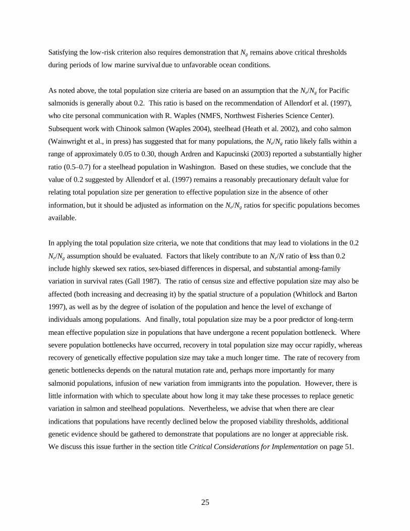
25

Satisfying the low-risk criterion also requires demonstration that Ng remains above critical thresholds

during periods of low marine survival due to unfavorable ocean conditions.

As noted above, the total population size criteria are based on an assumption that the Ne/Ng for Pacific

salmonids is generally about 0.2. This ratio is based on the recommendation of Allendorf et al. (1997),

who cite personal communication with R. Waples (NMFS, Northwest Fisheries Science Center).

Subsequent work with Chinook salmon (Waples 2004), steelhead (Heath et al. 2002), and coho salmon

(Wainwright et al., in press) has suggested that for many populations, the Ne/Ng ratio likely falls within a

range of approximately 0.05 to 0.30, though Ardren and Kapucinski (2003) reported a substantially higher

ratio (0.5–0.7) for a steelhead population in Washington. Based on these studies, we conclude that the

value of 0.2 suggested by Allendorf et al. (1997) remains a reasonably precautionary default value for

relating total population size per generation to effective population size in the absence of other

information, but it should be adjusted as information on the Ne/Ng ratios for specific populations becomes

available.

In applying the total population size criteria, we note that conditions that may lead to violations in the 0.2

Ne/Ng assumption should be evaluated. Factors that likely contribute to an Ne/N ratio of less than 0.2

include highly skewed sex ratios, sex-biased differences in dispersal, and substantial among-family

variation in survival rates (Gall 1987). The ratio of census size and effective population size may also be

affected (both increasing and decreasing it) by the spatial structure of a population (Whitlock and Barton

1997), as well as by the degree of isolation of the population and hence the level of exchange of

individuals among populations. And finally, total population size may be a poor predictor of long-term

mean effective population size in populations that have undergone a recent population bottleneck. Where

severe population bottlenecks have occurred, recovery in total population size may occur rapidly, whereas

recovery of genetically effective population size may take a much longer time. The rate of recovery from

genetic bottlenecks depends on the natural mutation rate and, perhaps more importantly for many

salmonid populations, infusion of new variation from immigrants into the population. However, there is

little information with which to speculate about how long it may take these processes to replace genetic

variation in salmon and steelhead populations. Nevertheless, we advise that when there are clear

indications that populations have recently declined below the proposed viability thresholds, additional

genetic evidence should be gathered to demonstrate that populations are no longer at appreciable risk.

We discuss this issue further in the section title Critical Considerations for Implementation on page 51.

26

Population Decline Criteria

Rationale: The population decline criteria address increased demographic risks associated with rapid or

prolonged declines in abundance to small population size. Populations that experience unchecked

declines may reach levels at which the probability of extinction from random demographic or

environmental events increases substantially (Soulé and Simberloff 1986), and if declines continue

unabated, deterministic extinction results. As defined by Allendorf et al. (1997), the criteria have two

components: a downward trend in population size (an indication that the population is not replacing itself)

and a minimum annual adult run size. Each of these components is evaluated in the context of the other.

Criteria: We adopt criteria consistent with Allendorf et al. (1997), with minor modifications. A

population is considered at high risk if it meets any of the following three conditions: (1) the population

has undergone a recent decline in abundance (within the last two generations) to an annual run size, Na, of

fewer than 500 fish; (2) the population currently has an average annual run size of Na > 500 but is

declining at a rate of $10% per year over the last two–four generations9, or (3) the population currently

has an annual average run size of Na > 500 but has been declining at a rate that, if it continued, would

cause Na to fall below 500 within two generations. In this high-risk category, the progeny/parent ratio is

less than one, indicating that populations are failing to replace themselves. Populations that have declined

to annual run sizes at or below 500 spawners but that are currently stable (i.e., progeny/parent ratio is ≥ 1)

or populations that are above 500 spawners but continue on a downward trajectory (i.e., progeny/parent

ratio is < 1) are considered at moderate risk of extinction. By extension, populations at low risk of

extinction are those with annual run sizes of greater than 500 and mean progeny/parent ratios of ≥ 1

(Table 1). Although Allendorf et al. (1997) do not specifically discuss their rationale for choosing 500

fish as the threshold between risk categories, we adopt their criteria to foster consistency between the two

approaches.

We note that the abundance threshold suggested by Allendorf et al. (1997) as indicative of high risk (Na <

500 spawners per year) is adopted as appropriate in the absence of information on intrinsic growth rate

(i.e., growth rate at low population density, when populations are released from intraspecific

competition). Population models that predict extinction probability can be highly sensitive to

assumptions about intrinsic growth rate and environmental stochasticity, which causes year-to-year 9 We note that it might be reasonable to argue that populations at high abundance (e.g., Na > 10,000 individuals) might experience declines on the order of 10% or more per year for two generations without appreciably increasing the risk of extinction. However, currently within the NCCC Recovery Domain, there is little evidence to suggest that any salmon or steelhead populations approach such abundances. Should such circumstances arise in the future, it would be appropriate to re-evaluate this element of the population decline criteria, particularly if information on potential sources of variation in population size is available.

27

variation in population growth rate (see e.g. Lande 1993; Foley 1994; Boughton et al. 2007). A

population with Na < 500 might have a relatively low probability of extinction if the intrinsic growth rate

were high and variation in growth rate low, but a high probability of extinction if the reverse conditions

were true. Consequently, relaxing this criterion would require demonstration that a population of fewer

than 500 spawners would not be at heightened risk of extinction10.

Metrics and Estimation: The population decline criteria require estimation of two parameters: mean

annual population abundance, aN , and population trend, T. We recommend using the geometric mean of

spawner abundance for the most recent 3–4 generations as an estimator for aN :

(3) nn

i iaNN geoma

/1

1 )()(

∏=

=

where Na(i) is the total number of adult spawners in year i, and n is the total number of years of available

data. The geometric mean is slightly more conservative than the arithmetic mean, in that low values have

greater influence on the mean. Mean spawner abundance should be based on counts of naturally

spawning fish, exclusive of hatchery-origin fish. Our recommendation to use this estimator is consistent

with analyses developed for previously published status reviews (e.g., Good et al. 2005).

Population trend, T, is estimated as the slope of the number of natural spawners (log-transformed)

regressed against time. To accommodate for zero values, 1 is added to the number of natural spawners

before log-transforming the value. The regression is calculated as follows:

(4) ln(Na + 1) = $0 + $1X +,

where Na is the annual spawner abundance, $0 is the intercept, $1 is the slope of the equation, and , is the

random error term (Good et al. 2005). Estimation of trend requires a time series of adult abundance for at

least two generations and up to four generations 11. It may be possible to estimate population trends using

indices of abundance, so long as the indices truly reflect overall population trends. However, as estimates

10 Results from Lindley (2003) suggest that a minimum of 30 years of data is likely needed to obtain unbiased estimates of variance in population growth rate within reasonable confidence limits. Such lengthy time series may be needed to accurately estimate variance when there are longer-term trends in abundance and productivity. 11 The population decline criteria are intended to capture recent, relatively rapid declines in abundance. Over longer periods of time, populations declining at less than 10% per year may still be at high risk of extinction. In the NCCC Recovery Domain, there are few existing time series of population abundance spanning longer than 10 years. In these cases, long-term trends should be evaluated independently of the proposed population decline thresholds.

28

0 10 20 30 40 50 60 70 80 90 100 110

Year

Abu

ndan

ce

Τ < 0

Τ >0

A.

B.

Figure 2. Hypothetical fluctuations in the abundance for a healthy population showing no long-term trend in abundance (A) versus a population undergoing a long-term decline (B). Thick lines depict periods where short-term population growth rates are in opposition to the long-term patterns. Figure based on a conceptual model by Lawson (1993).

of total abundance are needed to evaluate other criteria in Table 1, use of total population estimates will

generally be preferable to indices.

Interpretation of population trends is confounded by the fact that salmonid populations may undergo

natural fluctuations at time scales ranging from annual to decadal or longer, leading to highly variable

estimates of trend. As most estimates of T for populations of salmonids within the NCCC Recovery

Domain are likely to be based on relatively short time series of abundance, interpretation of T needs to be

made in the context of marine and freshwater survival during the period of record and other population

metrics of viability. For instance, healthy populations at little risk of extinction almost certainly

experience periods of negative population growth without being at heightened risk of extinction (Figure 2,

Line A). Conversely, populations experiencing a long-term downward trend in abundance may exhibit a

short-term positive trend response to periods of favorable ocean conditions (Figure 2, line B). These

scenarios underscore the need to both understand the causes of population fluctuations and to evaluate

population trend and abundance simultaneously, as short-term population trend by itself can be

misleading as a metric of viability. Our requirement that low-risk populations be stable or increasing also

considers the fact that the criteria proposed herein are being developed for ESUs that have already been

T > 0

T < 0

29

listed under ESA. In the vast majority of cases, most populations within these ESUs are considered

depressed, often severely so. In this context, it would seem unreasonable to conclude that a population

has recovered if it continues to decline in abundance. In future scenarios, demonstration that populations

can remain above viability thresholds for other population metrics (e.g., population size, effective

population size, and population density) during periods of both favorable and unfavorable conditions and

that the population responds positively and rapidly to improvement in marine conditions might justify

relaxation of the population trend requirement. In contrast, for populations that otherwise satisfy viability

criteria, short-term declines that lack an obvious mechanism (e.g., change in ocean conditions) would be

cause for renewed concern.

Catastrophe, Rate and Effect Criteria

Rationale: Catastrophes are large environmental perturbations that produce rapid and dramatic declines

in population abundance (Shaffer 1987; Lande 1993). Such events are distinct from environmental

stochasticity that arises from the continuous series of small or moderate perturbations that affect

population growth rate (e.g., interannual variation in climate, ocean conditions, food resources,

populations of competitors, etc.). Some population modelers have suggested that catastrophes may be

more important than either environmental or demographic stochasticity in determining average

persistence times of populations (Shaffer 1987; Pimm and Gilpin 1989; Soulé and Kohm 1989), though

Lande (1993) argues that the relative risks of environmental stochasticity and catastrophes cannot be

generalized, being dependent on the mean and variance of population growth rate and the magnitude and

frequency of catastrophes. Regardless, there is agreement that populations are at increased risk of

extinction following a major reduction in abundance.

Criteria: Within the Allendorf et al. (1997) framework, the goal of the catastrophe criteria is to capture

situations where a population has experienced a sudden shift from a no-risk or low-risk status to a higher

risk level. Allendorf et al. (1997) defined the very high-risk criterion for catastrophic declines as a 90%

decline in population abundance within one generation, and the high-risk criterion as “any lesser but

significant reduction in abundance due to a single event or disturbance.” These criteria depart to some

degree from the IUCN criteria (Mace and Lande 1991), which proposed average population reductions

over 2–4 generations of 50%, 20%, and 10% to correspond to critical, endangered, and vulnerable status,

respectively. Allendorf et al. (1997) offer limited discussion of the reasoning behind these differences,

noting only that Pacific salmonid stocks often exhibit substantial natural variation in abundance. We

surmise that Allendorf et al. felt that declines of the magnitude specified in the IUCN criteria may be well

30

within the range of natural variation for salmonid populations and thus adopted more stringent criteria.

Further, we note that the rates of decline listed in the IUCN criteria for catastrophic risk are generally

subsumed by the Allendorf et al. (1997) population decline criteria, which are adopted in this report.

We adopt the criteria of Allendorf et al. (1997) as they stand, considering populations that have

experienced a 90% decline in abundance within one generation to be at “high risk” of extinction and those

experiencing a lesser but significant decline to be at “moderate risk” (Table 1). Although Allendorf et al.

(1997) do not explicitly define what constitutes a “lesser but significant decline” in abundance, we

consider events such as the failure of a year class due to a catastrophic disturbance to be an example of

such an event.

Metric and Estimation: We define the estimator of catastrophic decline, C, as the maximum

proportional change in abundance from one generation to the next. Formally, this can be expressed as

follows:

(4)

=

− )2(

)(-1maximumˆhtg

tg

N

NC

where Ng(t) is the running generational sum of adult spawners in year t, and Ng( t-2h) is the running

generational sum at time t-2h, where h is mean generation time (rounded to the nearest whole year)12. By

this formulation, estimation of C requires a time series of adult spawner abundance of at least 3

generations (but see exception below), and should be based on naturally spawning fish, exclusive of

hatchery origin fish. As with the population decline criteria, it may be possible to evaluate catastrophic

declines using an index of abundance (rather than a total population estimate), provided that the index

faithfully reflects the characteristics of an entire population.

Although it may seem more intuitive to use the running sum in the most recent generation, N( t-h), in the

denominator of equation (3), the value of C is highly influenced by the pattern of abundance during the

transition from a period of high abundance to a period of low abundance since it is based on a running

sum of abundance. For example, consider the two time series of abundance depicted in Figure 3. Line A

illustrates a situation where population hovering around an average of about 50,000 spawners in years 1

through 13, drops in a single year to an average of about 5,000 spawners from year 14 to 30. Line B

illustrates the same scenario, but where the decline occurs over a generation (3 years), rather than in a

12 For example, for a coho salmon population with a mean generation time of three years, C at t = 9 would be 1 minus the sum of adult abundance for years 7, 8, and 9 divided by the sum of abundance for years 1, 2, and 3.

31

0

10000

20000

30000

40000

50000

60000

0 5 10 15 20 25 30

Year

Spa

wne

r A

bund

ance

A.

B.

Figure 3. Hypothetical example where an order of magnitude decline in abundance occurs over a single year (A) versus three years (B). See text for elaboration.

single year. Were N( t-h) used in the denominator, value of C would exceed the threshold (90%) only for

the scenario shown in line A, where the decline occurs over a single year. In scenario B, the intermediate

population abundances in years 14 and 15 effectively moderate the value of C , such that the 90%

criterion is never exceeded, despite the order of magnitude drop in abundance that occurred within 3

years. Use of N( t-2h) in the denominator assures that both scenarios are captured by the criteria.

We note that there may be instances where a population either exhibits a clear and precipitous decline in

abundance or suffers a major loss or alteration of habitat (e.g., landslide causing a passage blockage,

chemical spill affecting an entire year class, or some other catastrophic event). Clearly, in such cases, an

immediate elevated risk designation could be warranted, even in the absence of a longer time series of

data.

For longer time series where a population experienced a catastrophic decline in abundance at some time

during the past, consideration needs to be given to the response of the population following the

catastrophic decline. For example, in Figure 4, we depict three distinct trajectories in population

abundance following a catastrophe, including an increasing trend in abundance (Line A), a relatively

stable abundance (Line B), and a decreasing trend in abundance (Line C). Because the catastrophic

decline criteria are intended to capture heightened demographic risks associated with a rapid decline in

32

0

10000

20000

30000

40000

50000

60000

0 5 10 15 20 25 30 35 40 45

Year

Sp

awn

er A

bu

nd

ance

A.

B.C.

Figure 4. Hypothetical example catastrophic decline in abundance, showing three possible trajectories: A) apparent trend toward recovery from the decline, B) relatively stable abundance following the decline, and C) continued downward trend in abundance.

abundance, scenarios A and B are suggestive that, while the population did experience a rapid declines

exceeding the low-risk threshold, the population has since exhibited signs of stabilizing or increasing. In

such instances, the castastrophic decline criteria needs to be evaluated in the context of information on

patterns of marine survival or more-or-less permanent, naturally caused changes in system capacity (for

example, blockage of habitat due to a natural landslide or other disturbance where the blockage is

expected to persist for hundred or thousands of years).

Allendorf et al. (1997) provide no details about what might be considered a “lesser but significant decline

in abundance.” We conclude that the most likely occurrence that would qualify as a moderate risk of

extinction would be the loss or severe reduction in an individual year class due to a catastrophic

disturbance (e.g., fire, landslide, severe flood or drought, chemical spill, or some other similar

catastrophe). Because the risk associated with such an event is likely to vary substantially depending on

specific circumstances such as the size of the population in other year classes and the degree of life-

history variation (which influences how rapidly a population might recover from such a loss), we do not

propose numeric thresholds for moderate risk and instead suggest that such risk will need to be evaluated

on a case-by-case basis.

33

Spawner Density Criteria

Rationale: The spawner density element of the viability criteria is intended primarily to fill a perceived

gap in the Allendorf et al. (1997) framework with respect to population attributes identified as important

to persistence in the VSP framework: spatial structure and diversity. These characteristics of populations

influence viability by spreading risk through time and space and by contributing to the resiliency of

populations to natural and human-caused disturbances. Historically, populations making up an ESU

undoubtedly differed in average abundance as a function of differences in both the total habitat available

for spawning and rearing and the relative capacities of those habitats. Additionally, the distribution of

individuals across large and potentially diverse watersheds likely further enhanced the probability of

populations persisting over the long term. For example, populations where spawning occurs in multiple,

relatively discrete areas are less vulnerable to localized (reach or subwatershed) disturbances such as fires

or landslides and have greater potential to recovery from such disturbances, since unaffected portions of

the population can both sustain the population following the disturbance and provide colonizers to

repopulate the affected habitats. Further, populations distributed over a large watershed have the potential

to experience a broader range of environmental conditions, leading to greater phenotypic and genotypic

diversity. Life-history variation (e.g., variation in the age and size of individuals at smoltification and

maturity) potentially buffers populations from natural fluctuations in both freshwater and marine

conditions, spreading risk through both space and time (den Boer 1968; Hankin and Healey 1986; Hankin

et al. 1993; Mobrand et al. 1997; Hill et al. 2003). Greater genetic diversity increases the ability of a

population to adapt to changes in environmental conditions over the long term. As a population departs

from its historical pattern of distribution and abundance, through loss or degradation of habitat, the

probability of the population persisting decreases as well, though numerous factors will determine how

far a population can depart from historical conditions and still remain viable.

At the opposite end of the spectrum, populations that have been reduced due to severe and widespread

degradation of habitat may be subject to directional demographic processes that result in heightened

extinction risk. Specifically, at very low densities, populations may experience a reduction in per capita

growth rate with declining abundance, a phenomenon referred to as depensation. Most population growth

models typically assume that per-capita growth rate increases as population density decreases, a result of

reduced intraspecific competition. However, if populations are reduced to extremely low densities, a

variety of mechanisms can lead to reduced per-capita growth rate, including reduced probability of

fertilization (e.g., failure of spawners to find mates), inability to saturate predator populations, impaired

group dynamics, or loss of environmental conditioning (Allee 1931; Liermann and Hilborn 2001;

34

Montgomery et al. 1996). Depensation can result in a postitive feedback that, if unchecked, accelerates a

decline toward extinction.

High densities of spawning salmonids serve the additional role of providing marine-derived nutrients

from salmon carcasses, which help maintain the productivity of aquatic ecosystems. A growing body of

literature has documented the substantial contribution that salmon carcasses play in the nutrient budgets

of streams in the Pacific Northwest (Bilby et al. 1996, 1998, and 2001; Cederholm et al. 1999; Gresh et

al. 2000; Gende et al. 2002; Naiman et al. 2002; Schindler et al. 2003). Carcasses constitute important

sources of nitrogen and phosphorous, which fuel primary production in stream ecosystems, and provide a

direct source of food to juvenile salmon (Bilby et al. 1998). Reductions in abundance and spatial

distribution of salmonid populations may thus fundamentally reduce the capacity of the streams to

support salmonids, creating a feedback loop that could negatively affect long-term population persistence

or slow recovery. For example, Scheuerell et al. (2005) suggest that the reductions in the abundance of

spring/summer Chinook salmon in the Snake River basin may have resulted in a shift to a less productive

state, as evidenced by compensatory mortality in Chinook juveniles even though populations were far

below their historical abundance (Achord et al. 2003), as well as failure of smolt recruits per spawner to

rebound in years of higher adult abundance. Recognition of this important role has led to a growing call

for the link between salmon-derived nutrients and system productivity to be considered when setting

salmon recovery goals (Gende et al. 2002; Peery et al. 2003; Scheuerell et al. 2005). And though

additional research will be needed before escapement goals for ensuring maintenance of ecosystem (and

salmon) productivity based on nutrient subsidies can be established (Bilby et al. 1998; Gende et al. 2002),

requiring minimum spawner densities increases the likelihood that such benefits will be maintained or at

least not further eroded.

As fixed values, other metrics in the viability table (the effective population size criteria and population

size element of the population decline criteria) do not account for these historical among-population

differences in total habitat available for spawning and rearing, the relative productive capacity of those

habitats, the potential role of spatial structure and diversity in population persistence, the role of nutrient

subsidies in maintaining ecosystem productivity, or the possibility of depensation if individuals are

sparsely distributed across the landscape. It seems particularly problematic, for example, to conclude that

a population is viable at an Ne of about 500 (or Ng of 2,500) when historically that population was much,

much larger. An effective population size of 500 fish per generation in a small watershed might seem

reasonable, but a population with the same number of fish spread at low densities throughout a much

larger watershed could be at moderate or high risk of extinction. Even if the 500 fish per generation were

35

consistently concentrated in a core habitat within a watershed, reducing the risk of depensation, the risk of

extinction from a single catastrophe (e.g., flood, landslide, fire) would be higher. Equally important, in

either scenario the smaller population’s functional contribution to ESU viability would be substantially

diminished, even if the population remained viable.

We propose using criteria related to spawner density to address these issues of spatial structure and

depensation risk. In developing these criteria, we operate from the following set of assumptions:

• For independent populations, the historical distribution and abundance of adult spawners

represents reference conditions for which extinction risk was likely low and the population

made its greatest contribution to ESU viability. Under these conditions, populations likely

tended toward their carrying capacity, and the resilience imparted by spatial structure, diversity, and

ecosystem productivity (i.e., contribution of marine-derived nutrients) made it unlikely that the

population would go extinct in the absence of a large-scale catastrophe.

• The farther a population departs from its historical condition, the greater its extinction risk

and the higher the uncertainty associated with its viability13. Although some departure from

historical conditions due to diminished habitat quality or reduced spatial distribution (with

incumbent effects on diversity) may have minimal influence on population persistence, the more

restricted and/or fragmented the distribution of the population becomes, the higher its extinction

risk.

• How far a population can deviate from its historical condition and remain viable depends, in

part, on how large the population was and how it was distributed historically. Thresholds

defined for the minimum amount of intrinsic habitat potential (IPkm14) required for viability in

isolation are based on an assumption that, under historical conditions, populations were at or near a

carrying capacity. For historically small populations (i.e., those near the IP threshold for

independence), reductions in abundance or distribution would likely move these populations below

levels required for viability. For populations in larger watersheds, a comparable percentage

reduction in habitat is less likely to result in a substantial increase in extinction risk.

13 Theoretically, human modifications that increased the amount of available habitat, such as construction of fish passage structures around natural barriers, could constitute an exception to this generalization. 14 IPkm is an estimate of the accessible stream kilometers, weighted by their intrinsic potential, as estimated by the model of Burnett et al. (2003) and modified by Agrawal et al. (2005). See Bjorkstedt et al. (2005) for details.

36

• At extremely low densities, populations may be at heightened risk of extinction due to

depensation. Although demographic and environmental variability can make it very difficult to

detect depensation in fish populations, the consequences of depensation are sufficiently severe to

warrant consideration of depensatory processes when populations are at very low densities.

The first three assumptions relate directly to the establishment of low-risk thresholds, where the key

question is “how far can a population depart from historical conditions and still remain viable?” This is a

difficult question to answer, given that the quantitative basis for relating spatial structure, diversity, and

ecosystem productivity is presently limited. The last assumption deals directly with establishment of a

high-risk threshold, where the key question is “at what densities is depensation likely to occur in salmonid

populations?” This too is a challenging question, as detecting depensatory processes in natural

populations has proven difficult, though not impossible. Despite these acknowledged uncertainties, the

NCCC TRT believes that reasonable criteria can be developed from these general principles.

Criteria: The spawner density criteria define two thresholds. The first, which distinguishes between

populations at high versus moderate risk, is based on potential depensation effects. The second defines

the threshold between moderate and low risk based on spatial structure, diversity, and productivity

concerns. Populations potentially at high risk of depensation are defined as those with average spawner

densities of fewer than 1 adult spawner per IPkm. For the low-risk threshold, we propose density criteria

that vary as a function of both species and population-specific estimates of potential habitat capacity

(Figure 5).

For the smallest watersheds capable of supporting viable populations (as estimated based on IPkm), low-

risk populations are defined as those exceeding 40 spawners per IPkm, a value assumed to approximate a

natural carrying capacity for salmonids systems (see discussion below). For larger watersheds, required

densities decrease to a minimum of 20 spawners/IPkm (Figure 5) based on the assumption that larger

populations can depart farther from historical conditions before extinction risk is substantially increased.

Defining the density at which depensation is likely to occur is difficult due to high variability and few

observations at low abundances in most spawner-recruit datasets (Liermann and Hilborn 1997, 2001).

Nevertheless, several authors have attempted to define thresholds at which depensation appears to occur

in salmonids. Based on spawner-recruit data for coho populations, Barrowman (2000; cited in Chilcote et

al. 2005 and Wainwright et al., in press), suggested that depensation may become a factor at spawner

37

Available IPkm

0 100 200 300 400 500 600

Coho salmon

Moderate Risk

Sp

awn

er D

ensi

ty (a

du

lts/

IPkm

)

0 100 200 300 400 500 600

05

1015202530354045

Low Risk

Moderate Risk

High Risk

Chinook salmon

Spa

wne

r D

ensi

ty (

adul

ts/IP

km)

05

1015202530354045

0 100 200 300 400 500

05

1015202530354045

Spa

wne

r D

ensi

ty (

adul

ts/IP

km)

Steelhead

Low Risk

Moderate Risk

High Risk

32

20

16

Low Risk

600

High Risk

Figure 5. Relationship between risk and spawner density as a function of total intrinsic habitat potential

for coho salmon, Chinook salmon, and steelhead. Values above upper lines indicate populations at low risk; values below this line are at moderate risk. Values below 1 spawner/IPkm are at high risk for all species. Dashed vertical lines indicate minimum IPkm for independent populations.

38

densities of 1 female per km. Likewise, Barrowman et al. (2003) found little evidence of depensation in

coho salmon unless densities were less than 1 female/km. Assuming a 50:50 sex ratio, these values

equate to 2 adults per km. Based on analysis of coho populations that went extinct in the lower Columbia

River during the 1990s, Chilcote (1999) suggested that populations were unlikely to recover if their

densities fell below about 2.4 adults/km. Similarly, Sharr et al. (2000) suggested that coho populations at

densities of fewer than 2.4 adults per km should be considered “critical” based on potential risks of

depensation. Based on these data, the OCTRT (Wainwright et al., in press) concluded that depensation

risks were very likely at spawner densities of 0.61 spawners per km (1 spawner per mile). For our

purposes, we chose to use IPkm in the denominator in order to account for potential differences in habitat

quality among watersheds15. Since the ratio of IPkm to total km is about 0.6 for coho salmon, the OCTRT

rule of 0.6 fish per km equates to approximately 1 fish per IPkm, the criterion we propose. In adopting

this criterion, we recognize that the empirical evidence supporting depensation in salmonid populations

remains somewhat limited. However, we heed the recommendation of Liermann and Hilborn (2001) who

noted that the paucity of evidence “should not be interpreted as evidence that depensatory dynamics are

rare or unimportant.” In practical application of our population viability criteria, the depensation criterion

is likely to play a significant role in population risk classification only for the largest populations within

the domain, as other criteria (e.g., effective population size, and population decline criteria) are likely to

be more conservative in watersheds where potential habitat is estimated to be less than 500 IPkm.

The low-risk density criteria were defined based on the following rationale. First, recall that for each

species, Bjorkstedt et al. (2005) defined a minimum threshold of potential habitat (expressed as IPkm)

that was required for the population to be considered viable -in-isolation (32 IPkm for coho salmon, 20

IPkm for Chinook salmon, and 16 IPkm for steelhead), with the among-species differences in IPkm

thresholds reflecting differences in life-history variation. These thresholds assume that populations

historically operated at something close to the natural carrying capacity of the system. By extension, for

populations in the smallest watersheds (in IPkm terms) capable of supporting a viable population to

remain viable, they must function at something close to this historical carrying capacity, as any reduction

in abundance would drop them below thresholds for viability. Consequently, the average spawner density

at natural carrying capacity serves as a reasonable basis for establishing the threshold for low-risk in the

smallest watersheds.

15 The decision to use IPkm was based on an assumption that IPkm provides a reasonable measure of the relative productive potential of a watershed. For watersheds that have comparable IPkm but somewhat different total km, the average density, expressed as fish/km might be expected to be lower in the less productive watershed, potentially leading to greater depensation risk. However, we assume that in most cases, fish distribute themselves somewhat according to habitat quality; thus, we consider these two scenarios as having comparable risk.

39

The difficulty lies in estimating this value. For coho salmon, we relied on the work of Bradford et al.

(2000), who examined stock-recruit relationships for 14 historical data sets of coho salmon in the Pacific

Northwest. Fitting a hockey stick model to these data, they found that, on average, the plateau in the

stock-recruit relationship, which identifies number of spawners at which full smolt recruitment occurs (an

estimate of carrying capacity), occurred on average at 19 females per kilometer. Assuming a sex ratio

that is slightly biased in favor of males, we round this number to approximately 40 adult spawners per

kilometer. For Chinook salmon and steelhead, we lack the same kind of empir ical basis for setting the

spawner density for watersheds with the minimum IP required for viability, and so we default to the 40

spawners/km value recommended for coho salmon.

For coho salmon, we find some support for our recommended spawner density in population viability

models developed for coho salmon on the Oregon Coast. Recall that the NCCC TRT estimated that at

least 32 IPkm was required for a population of coho salmon to be considered viable -in-isolation

(Bjorkstedt et al. 2005). This threshold value was based on the simulation analyses of Nickelson and

Lawson (1998), who used a life-cycle model to predict extinction risk for a population of coho salmon as

a function of the amount of “high quality” habitat available (Bjorkstedt et al. 2005). The Nickelson-

Lawson model produces quantitative extinction probabilities. These probabilities are sensitive to many of

the model parameters; thus, determining an absolute extinction probability for any population is difficult.

Nevertheless, the model consistently shows that extinction probabilities begin to rise rapidly when the

available high-quality habitat falls below 24 kilometers. The NCCC TRT set the viability-in-isolation

threshold based on an assumption that watersheds with at least 32 IPkm would have sufficient high-

quality habitat to support a viable population (Bjorkstedt et al. 2005). These estimates assume that this

quantity of habitat would be expected to produce sufficient numbers of smolts to yield 1,500 spawners

during a period of 1% marine survival (Wainwright et al., in press). For the smallest population (i.e., in a

watershed with 32 IPkm), 1,500 spawners would result in a density of about 47 spawners per IPkm, a

value in reasonable agreement with the 40 spawners/IPkm chosen for our criteria.

For Chinook salmon the default value of 40 spawners/km value is consistent with the rationale of

Bjorkstedt et al. (2005). Based on reported values for average Chinook salmon redd densities, they

argued that a redd density of 20 per km (and thus a spawner density of 40 fish/km assuming a 50:50 sex

ratio) over 20 IPkm would be required for a population to be viable. We also note that although the

density required for viability in the smallest watersheds is the same for coho salmon, Chinook salmon,

and steelhead, the absolute abundance requirements would differ, since the IPkm threshold for viability

40

differs (i.e., the smallest watershed for viable coho salmon, Chinook salmon, and steelhead populations

would require annual run sizes of 1,280, 800, and 640 spawners, respectively). This result is consistent

with the hypothesis that the greater life-history diversity exhibited by steelhead and Chinook salmon

enables them to persist at somewhat lower absolute abundances than coho salmon, which have a more

rigid life history.

With the spawner density criteria of 40 fish/IPkm for the smallest populations serving as an anchoring

point, the next step was to generate a function representing our general conclusion that the larger the

population historically was, the more it can depart from historical conditions and still remain viable.

Here, we assume that a population with ten-fold more habitat potential than the smallest population

requires an average spawner density half that of the smallest population and that the required density

declines linearly between these two reference point (Figure 5). For watersheds with greater than ten-fold

the habitat potential of the minimum watershed, we assume that spawner density must be at least 20

fish/IPkm for the population to be at low risk.

We acknowledge that selection of the latter reference point is based largely on expert opinion and that

there is room for debate about both the shape of the density function and the floor density that is used for

large watersheds. However, we believe that application of the density criteria yields results that are

qualitatively consistent with general hypotheses relating watershed size and density to spatial structure,

diversity, and other factors that influence population persistence. First, a result of application of the

density criteria is that it establishes a watershed-specific abundance target that is scaled to the amount of

potential habitat. This overcomes the unsatisfying outcome of “fixed” abundance criteria, where a

remnant of a historically very large population might still be considered “viable” in the sense of having a

low extinction risk over some time frame, even though the population clearly plays a much-diminished

role in ESU viability. A second desirable outcome is that the density criteria substantially increase the

likelihood that elements of spatial structure and diversity that contribute to viability will be maintained,

without rigidly asserting what that spatial structure must look like. For example, in a large watershed, the

density criteria could be attained in a variety of ways, ranging from having roughly half the available

habitat occupied at something near carrying capacity, with little use of remaining habitats, to having fish

distributed at moderate densities throughout the watershed. Each of these scenarios offers some potential

advantages and disadvantages from a population persistence standpoint. For example, populations

anchored in a subset of watersheds that are functioning at or near carrying capacity may provide for

greater resilience during periods of low ocean productivity (Nickelson and Lawson 1998) but be at

somewhat more risk of localized disturbances than populations distributed more broadly but at lower

41

average densities. Because these tradeoffs do not seem to be quantifiable given our current state of

knowledge, the density criteria seem preferable to more stringent requirements related to spatial structure.

Metrics and Estimation: For the high risk of depensation threshold, we propose estimating average

spawner density (expressed as spawners/IPkm) in the h consecutive years of lowest abundance within the

last four generations, where h is mean generation time for the species. Mathematically, we express this as

follows:

(5) IPkmh

ND tg

dep

= )(minˆ

where Ng(t) is running generational sum of spawner abundance at time t, and IPkm is the estimate of

potential habitat capacity for the watershed in which the population resides (see Chapter 4 for IPkm

estimates for each independent population). The decision to evaluate average spawner density in the h

consecutive years of lowest abundance (as opposed a single year or over all years) balances several

considerations. Foremost, we seek an indicator that is sensitive to the possibility that a population is at

risk of depensatory mortality, without being overly sensitive to natural fluctuations in abundance. For

example, a population that experiences a single year of low abundance may be at minimal risk of slipping

into an accelerating pattern of depensation, especially for species with overlapping generations, which

may be able to rebound more rapidly after a poor year. On the other hand, a metric that uses average

abundance over a longer period could be insensitive to depensation risks if a few relatively good years

elevate the average to levels above the depensation threshold and thereby mask these risks. Selecting the

lowest h consecutive years looks for recurring evidence of population numbers sufficiently low that there

is heightened potenential for depensatory dynamics that could rapidly deteriorate into a feedback

situation. We note also that the proposed metric assumes that fish are distributed relatively uniformly

across the available spawning habitats. Were spawner densities consistently higher in certain locations

within a watershed, it would suggest that risks associated with depensation due to the difficulty of

spawners finding mates might be low and that the criterion could therefore be relaxed, though other

possible depensation mechanism (e.g., lack of predator saturation) must also be considered.

For the low-risk density threshold, we propose as a metric the arithmetic mean of adult spawner density,

expressed as adult spawners per IPkm, for all years over the last four generations:

42

(6) ∑=

=h

t

assd

IPkmN

hD

4

141ˆ

where Na and IPkm are as defined above, and h is the mean generation time for the population (rounded to

the nearest whole year). The estimated density is then evaluated against thresholds that are a function of

both species and populations-specific estimates of potential habitat capacity or IPkm, as outlined in Figure

5.

Density estimates are likely to be derived in two different ways. First, where weirs or other fish passage

structures exist, average density can be estimated by dividing either total fish count (if all upstream

migrating fish are captured) or a total population estimate (if only a portion of adults are captured, but

where the proportion can be accurately estimated)—both of which estimate annual run size, Na—by the

number of stream IPkm accessible in the watershed. Second, where randomized spawner surveys allow

for population estimation, again the total population estimate, Na, can be divided by total accessible IPkm

in the basin to yield an average density over the entire watershed.

Of the criteria proposed in this document, the density criteria perhaps generated the most discussion

among TRT members about both the selection of the specific criteria and the most appropriate way to

apply them. Among the specific issues debated were (1) the relationship between density and viability in

populations where a significant amount of historical habitat is now inaccessible behind dams or severely

degraded (which becomes a question of selecting an appropriate habitat-based denominator when

estimating density); (2) whether the proposed criteria were sufficiently precautionary or overly so; (3)

whether it was more appropriate to express density criteria in terms of fish per IPkm or fish per total

accessible kilometers; and (4) whether adjustments to the criteria should be made to account for potential

bias in estimates of IP. We discuss the first of these issues in the paragraphs that follows, since resolution

of this issue is integral to subsequent discussion of ESU-level viability criteria that comes in Chapter 3.

The remaining topics we treat in Appendix B.

An important issue in estimating density is how to handle situations where substantial historical habitat

now lies behind impassible dams or other human-caused barriers to fish migration. This raises the

question as to whether, in estimating density using the two methods above, it is more appropriate to use

historical versus currently available IPkm in the denominator. In some instances, where significant

historical habitat has been lost, use of historical IPkm would, in all likelihood, preclude such populations

from ever attaining viable status in relation to historical standards. This seems problematic, in that there

43

may be sufficient habitat downstream of impassible barriers (i.e., more than the minimum threshold for

the population to be considered viable in isolation) to support a viable population. (Put another way, it

seems illogical to conclude that a population below human-created barriers that still has access to

substantial habitat cannot be viable, if a population in a watershed with comparable habitat but no such

barriers can be considered viable.) On the other hand, excluding areas upstream of barriers from

consideration violates one of our fundamental assumptions: that the spatial structure and diversity

resulting from the distribution of individuals broadly and over diverse habitats contributes significantly to

population persistence. We therefore recommend that populations be evaluated based on both historical

(pre-barrier) and current (post-barrier) conditions. Populations that fail to satisfy density criteria based on

historical habitat availability but that do satisfy the density criteria as applied to current conditions could

potentially be considered viable in the sense of having a relatively high probability of persistence. But

these “partial populations” represent something other than the historically defined population. Such

populations could be at greater risk than if criteria for the historical habitat were met (due to loss of

diversity or spatial structure), and their contribution to ESU persistence might be substantially

diminished, requiring reassessment of their role in ESU viability.

A related issue is how to deal with situations where fish still have access to portions of a watershed, but

where habitat alterations are both severe and permanent (e.g., intensive urbanization), effectively

precluding use by salmonids. In principle, arguments similar to those discussed above could be used to

make the case that density should only be estimated in those habitats that still are capable of supporting

salmonids. However, whereas in the case of dams, habitat losses are relatively easy to quantify, habitat

degradation is a matter of degree, and thus defining boundaries around areas that are no longer suitable

becomes problematic. We conclude that, assuming such areas could be clearly defined16, one could

evaluate density criteria using only “accessible and suitable” habitats; however, again such “partial

populations” represent something other than the historical population, having substantially departed from

their historical spatial structure and diversity. In no case should a population be considered viable, by any

standard, when the remaining habitat that is deemed suitable does not meet the minimum viability

thresholds set for each species (i.e., 32 IPkm for coho salmon, 20 IPkm for Chinook salmon, and 16 IPkm

for steelhead). How “partial populations” may relate to viability at the levels of diversity strata and ESUs

is discussed further in Chapter 3.

16 Defining such areas may be complicated if fish from relatively good habitats periodically “leak” into poor habitats.

44

Hatchery Criteria

Rationale: The hatchery criteria are intended to address potential impacts of hatchery operations on the

viability of wild populations of salmon and steelhead. Hatchery operations can affect wild populations

through a variety of ecological, demographic, and genetic mechanisms, thereby influencing their

probability of persistence.

The potential ecological effects of hatchery operations and hatchery fish on wild fish are many and

varied. When released into the wild, hatchery fish may compete for food, space, or mates with wild fish

in both the freshwater (Nickelson et al. 1986) and marine (Levin et al. 2001; Ruggerone et al. 2003;

Ruggerone and Nielsen 2004) environments. Hatchery fish can alter predator-prey dynamics by preying

directly on wild salmonids (Sholes and Hallock 1979) or by attracting or supporting increased numbers of

avian, mammalian, or piscine predators, resulting in increased predation rates on wild fish (Collis et al.

2001; Ryan et al. 2003; Major et al. 2005). Conditions within hatcheries can increase the vulnerability of

fish to infection by pathogens, cause pathogen amplification, and increase opportunities for disease

transmission (Moffitt et al. 2004). These diseases can then be transferred to wild populations (Kurath et

al. 2004). Marine or estuarine netpen rearing of such hatchery fish can also result in transfer of pathogens

and parasites to nearby wild fish (Naylor et al. 2005; Krkosek et al. 2006). Stocking of large numbers of

hatchery smolts in streams containing wild fish can also alter the behavior of wild fish, resulting in

premature emigration of wild fish (Hillman and Mullan 1989). Additionally, hatchery facilities

themselves may pose risks to wild populations by diverting water from natural streams in order to supply

hatcheries, releasing polluted effluent (e.g., fish wastes, antibiotics) waters from hatcheries back into

streams and rivers, and creating barriers to migration through installation of weirs or other fish collection

structures (White et al. 1995; Pearsons and Hopley 1999; Reisenbichler 2004).

Hatchery programs also potentially pose direct demographic risks to wild populations. Production of

large numbers of hatchery fish can result in increased human harvest of wild fish in mixed-stock fisheries,

resulting in reduced spawning escapement (McIntyre and Reisenbichler 1986; Hilborn 1992; NRC 1996;

Reisenbichler 2004). Additionally, hatchery programs that draw broodstock from wild populations, so-

called broodstock mining, also pose direct demographic risks to the wild population if the survival and

subsequent reproductive success of hatchery-origin fish that spawn in the wild does not at least replace

production lost due to the removal of natural-origin fish for broodstock (ISAB 2003). Broodstock mining

may also compromise the ability of a wild population to maintain its genetic character if too few adults

are allowed to spawn naturally, increasing the risk for adverse effects associated with small population

size (effects that may be exacerbated if broodstock suffer a catastrophic loss in the hatchery). In very

45

small populations, removal of wild fish for hatchery broodstock may result in depensation, through Allee

effects and other mechanisms, in the remaining wild population if too few individuals are left to spawn.

Genetic risks of hatcheries arise when wild fish interbreed with genetically dissimilar hatchery fish, which

can result in changes in genetic composit ion of wild populations, as well as genetic structure across larger

spatial scales. Under natural conditions, accurate homing to natal streams tends to result in the formation

of distinct breeding groups or populations that, over time, become locally adapted to the environmental

conditions they experience during their life cycle. This local adaptation and the diversity it creates over

larger spatial scales are important for the long-term persistence of populations and ESUs (NRC 1996;

Hendry 2001; McElhany et al. 2000; Reisenbichler et al. 2003). Within populations, interbreeding of

wild fish with hatchery-origin fish can alter the genetic characteristics of the wild population, reducing the

(average) individual fitness and hence overall population productivity (ISAB 2003). When hatchery fish

stray into other watersheds and interbreed with wild fish, patterns of genetic variation can likewise be

altered.

Genetic differences between hatchery and wild populations can arise in several non-mutually exclusive

ways. First, they may result when nonnative (i.e., out-of-basin or out-of-ESU) broodstock are used in the

hatchery. Second, genetic differences can arise when hatchery broodstock are subject to various artificial

selection processes, sometimes referred to as domestication selection, that result either through hatchery

practices or from exposure to unnatural hatchery environments. Artificial selection processes may be

intentional, such as when hatchery managers select for certain desirable traits (e.g., size of broodstock or

progeny, timing of return, etc.) or inadvertent, such as when selected broodstock randomly differ in some

trait from wild populations or when the hatchery environment favors (and therefore selects for) traits that

improve survival in the hatchery but that may lead to reduced fitness in the wild. And third, genetic

modification may occur through hybridization of distinct subspecies, races, runs or phenotypes that co-

occur in the same stream or basin. For example, hybridization of spring- and fall-run Chinook in the

Feather and Trinity rivers appears to have occurred in response to broodstock collection during periods of

overlap in run timing (Blankenship et al., in prep; Kinziger et al., in review). Regardless of the specific

mechanism, the result is hatchery populations that differ in their genetic composition from wild

populations.

Another genetic risk of hatcheries is the "Ryman-Laikre effect", whereby the admixture of hatchery fish

into a natural population causes a reduction in the effective population size of the combined population

(Ryman and Laikre 1991). This occurs because a group of hatchery fish generally have a smaller number

46

of parents than a similar-sized group of natural fish, due to higher juvenile survival within the hatchery.

When these hatchery fish reach reproductive age and interbreed with wild fish, the average number of

genetic lineages in their offspring will be lower than if they were all wild fish. The magnitude of the

reduction in effective size is proportional to the percentage of spawners that are hatchery fish and the

difference in the average number of parents for the hatchery and wild fish.

Of particular concern within hatchery broodstock is inbreeding depression, which is when interbreeding

between closely related individuals causes a decrease in average fitness of offspring, usually resulting

from increased frequency of homozygotes for deleterious recessive alleles, fixation of deleterious alleles

within a population, or loss of overdominance. Outbreeding depression is a reduction in fitness of hybrid

progeny when genetically dissimilar fish interbreed. It can result when wild fish interbreed with

nonnative (e.g., out-of-basin or out-of-ESU) fish or when wild fish interbreed with hatchery fish that have

undergone domestication selection. Processes that contribute to outbreeding depression include the

introduction of alleles from the hatchery stock that are maladaptive in the local environment or the

breakdown in co-adapted gene complexes (Fleming and Petersson 2001; ISAB 2003). Evolutionary

models suggest that genetic exchange between hatchery fish and wild fish has the potential to erode the

fitness of wild populations, with effects depending on the strength of selection and the magnitude of the

hatchery contribution to total production (Ford 2002; Goodman 2004, 2005). Such changes may occur

even if a large proportion of the hatchery broodstock consists of natural-origin fish (Ford 2002).

Collectively, these processes can result in a variety of population-level and ESU-level changes in genetic

diversity, including decreased within-population diversity resulting from insufficient numbers of

broodstock and inappropriate mating protocols; loss or dilution of distinct, locally adapted populations;

and increased homogenization of populations within an ESU (through increased straying). Such changes

may affect the long-term persistence of both populations and the ESUs comprising those populations.

Although the ecological, demographic, and genetic effects of hatcheries on wild populations are well

documented (see NRC 1996 for a review), quantitatively relating these effects to the probability of

extinction of populations is difficult. Many of the ecological impacts of hatcheries are highly context-

dependent. For example, competitive interactions between hatchery and wild fish are likely to vary with

the carrying capacities of different ecosystems, the size of the wild population at the time of introduction,

the number of hatchery fish released, the average size of stocked fish relative to wild fish, whether fish

are planted in a few locations or distributed broadly across a watershed, or any number of other

confounding factors. Likewise, genetic impacts on wild populations will depend on many factors

including the origin of broodstock, how the hatchery is operated (e.g., mating protocols, rearing

47

practices), and the number and effectiveness of hatchery fish that spawn in the wild, among other things.

Further complicating matters in the NCCC Recovery Domain is the fact that hatchery programs at many

facilities have changed substantially in the past decade or so, from predominately large-scale production-

oriented programs to smaller-scale supplementation or captive broodstock programs. For example, out-

of-basin coho salmon were planted for a number of years in the Russian River basin; however, the

program was terminated in the mid 1990s, and there is now a captive broodstock program in operation

intended to conserve what appears to be a remnant native population. Consequently, assessing potential

hatchery risks involves evaluating not only current practices, but potential lingering genetic effects

resulting from historical operations as well.

Criteria: Because of the numerous and complex ways in which artif icial propagation activities may

affect wild populations of salmonids, and because of the unique histories of ongoing and recently

terminated hatchery programs within the recovery domain, the NCCC TRT concluded that simple

numeric criteria for assessing hatchery risk would be difficult to justify. Acknowledging both the

potentially significant risks that hatcheries pose to wild populations and the uncertainty in quantitatively

relating these risks to extinction risk, the NCCC TRT adopts the following narrative criteria for

hatcheries: populations are considered at low risk if there is demonstrably no or negligible evidence for

ecological, demographic, or genetic effects resulting from current or past hatchery operations; populations

are at elevated risk (moderate-high) if there is evidence of significant ecological, demographic, or genetic

effects or high uncertainty surrounding these potential effects (Table 1).

The NCCC TRT notes that other Technical Recovery Teams have developed quantitative criteria

specifically addressing genetic risks of hatcheries. For example, the OCTRT (Wainwright et al., in press)

and Southern Oregon-Northern California Coast TRT (Williams et al., in prep.) propose assessing genetic

risk based on the fraction of natural spawners that are of hatchery origin. The Interior Columbia (ICTRT

2005) and Central Valley TRT (Lindley et al. 2007) propose a somewhat more complicated approach in

which risk is assessed based on the fraction of natural spawners of hatchery origin in relation to the

degree of genetic divergence between hatchery and wild stocks, the management practices used at the

hatchery, and the duration of interaction between hatchery and wild populations.

We considered using such approaches but concluded, for the reasons noted above, that few hatchery

programs (current or recent) could be effectively evaluated by those criteria, and that case-by-case

assessment of hatchery impacts is more appropriate for the NCCC Recovery Domain. Nevertheless, from

these documents and others, we have drawn a number of important principles that can assist in guiding

48

such assessments of risk. These principles are discussed in Metrics and Estimation below. Our decision

not to adopt numeric criteria, as done by other TRTs, should not be construed as contradictory, but instead

reflects substantial differences in the number and types of hatchery programs found in the different

recovery domains. Within other recovery domains, existing programs are predominately large-scale

production hatcheries that have been operated for many decades. In contrast, only two large-capacity

production hatchery programs (Mad River and Warm Springs/Coyote Valley steelhead) are currently

operating within the NCCC domain, the remainder being conservation hatcheries (e.g., captive broodstock

programs) or small-scale cooperative supplementation hatcheries (Table 3).

Metrics and Estimation: Because analysis of risks associated with hatcheries should be done on a case-

by-case basis, we do not propose specific metrics for assessing risk. To a substantial degree, the types of

risks and hence the associated risk indicators depend on the type of hatchery program being considered.

The Hatchery Scientific Review Group (HSRG 2004; Mobrand et al. 2005) suggests that, for the purposes

of assessing risk, it is useful to distinguish between two types of hatchery programs based on management

goals and protocols for propagating the hatchery broodstock. Integrated hatchery programs seek to

minimize genetic divergence between the hatchery broodstock and a naturally spawning wild populaton

by systematically incorporating wild fish into the hatchery broodstock. Segregated hatchery programs, in

contrast, strive to maintain hatchery broodstock that are distinct from their wild counterparts by using

predominately or exclusively hatchery-origin adults returning to the hatchery in subsequent broodstock.

These general categories can be further subdivided based on the specific purposes of the hatchery (e.g.,

harvest augmentation, supplementation, restoration, rescue, etc.). The specific genetic, demographic, and

ecological risks associated with various hatchery program types will differ, as can the approaches for

minimizing such risks and the data needed for risk evaluation. We provide general guidance on issues

that should be considered when evaluating risks associated with hatcheries, the types of information that

are needed to evaluate these risks, and some basic principles that can inform risk assessment in Appendix

C of this report. Without a thorough evaluation of hatchery risks, populations affected by hatcheries

should generally be considered at risk because of the high uncertainty surrounding these potential effects.

Summary of Population Metrics and Estimators

Most of the metrics for evaluating populations against the proposed population viability criteria require

time series of adult spawner abundance spanning three to four generations (but see preceeding discussion

for possible use of abundance indices for estimation of population trends and catastrophic declines).

Table 4 presents a summary of the metrics proposed in this paper and the data needs for estimating each.

49

Table 3. Current salmon and steelhead hatchery programs operating within the NCCC Recovery Domain, their purpose, mode of operation, and status.

Species, facility, and agency

River basin

Program type

Years of operation

Description and status

Chinook salmon Hollow Tree Creek (Eel River Restoration Project)

South Fork Eel River

Supplementation 1983 to present

Supplementation program that uses local broodstock to boost populations in Hollow Tree Creek, tributary to the South Fork Eel River. Development of hatchery genetic management plan ongoing.

Coho salmon Don Clausen Warm Springs (CDFG)

Russian River Rescue/captive broodstock and restoration

1979 to present; captive broodstock since 2001

Historically a production program that used out-of-basin and out-of -ESU (primarily Noyo River) fish for broodstock. Captive broodstock program was initiated in 2001; juveniles are collected from tributaries (Green Valley Creek) are reared to the adult stage at the hatchery and then spawned. Juveniles are subsequently released into Russian River tributaries to re-establish depleted or extirpated subpopulations.

Big Creek (Monterey Bay Salmon and Trout Project)

Scott Creek Rescue/captive broodstock, restoration, and supplementation

1982 to present; captive broodstock since 2001

Historically a supplementation program. Currently, a combined supplementation/captive broodstock/ restoration program. Broodstock are collected from Scott Creek; broodstock collection is prioritized so that only wild fish are taken in strong year classes, returning hatchery fish are used if wild fish are unavailable, and captive broodstock are used as last resort. Progeny are released into Scott Creek for supplementation, as well as in other watersheds to re-establish depleted or extirpated populations.

Steelhead Mad River winter steelhead (Friends of Mad River/CDFG)

Mad River Production 1971 to present

Historically operated as a production program to support fisheries that was established with out -of-basin (Eel River) broodstock. Currently operating as a cooperative hatchery with a goal of releasing 150,000 yearlings annually. Development of hatchery genetic management plan ongoing.

Warm Springs/ Coyote Valley winter steelhead (CDFG)

Russian River Production 1982 to present

Large-scale production program with goal of releasing 300,000 yearlings annually from Warm Springs and 200,000 yearlings from Coyote Valley. Some history of out -of-basin transfers (Eel and Mad River fish) pre-dating hatchery construction and continuing to the early 1990s (Busby et al. 1996). Development of a hatchery genetic management plan ongoing.

Big Creek winter steelhead (Monterey Bay Salmon and Trout Project)

Scott Creek/ San Lorenzo River

Supplementation 1982 to present

Supplementation program that uses local broodstock to boost populations in Scott Creek and the San Lorenzo River. Historically involved outbasin planting, but in recent years Scott Creek and San Lorenzo River fish have been planted only in their stream of origin.

50

Table 4. Estimation methods and data requirements for population viability metrics. Note that all references to population abundance refer to naturally produced adults (i.e., exclusive of hatchery returns).

Population Characteristic

Metric

Estimator

Data Needs

Effective population size per generation

-or-

Total population size

per generation

eN

)(harmgN

Variable: several direct and indirect methods for estimating Ne (see text). Harmonic mean of spawner abundance per generation:

∑=

=n

t tg

harmg

Nn

N

1 )(

)( 11

1

*

where n is the number of years, where Ng(t) is the running sum of adult abundance over period equal to the population’s mean generation time (rounded to the nearest whole year) at time t*

Variable Time series of adult spawner abundance, Na, for a minimum of 4 generations; demonstration that Ng remains above threshold during periods of low marine survival

Population decline Critical run size

)(geomaN

Geometric mean annual adult run size:

nn

i iaNN geoma

/1

1 )()(

∏=

=

Time series of adult spawner abundance, Na, for a minimum of 4 generations; demonstration that Na remains above threshold during periods of low marine survival

Population trend T Slope of natural log of the g-year running sum of abundance v. time:

T = slope ln(Na+1) v. time

where Na is as defined above

Time series of adult spawner abundance, Na, for 2-4 generations; demonstration that increasing trend is not result of short-term increases in marine survival

Catastrophic decline C Maximum 1-generation decline (proportion) in abundance:

=

− )2(

)(-1maximumˆhtg

tg

N

NC

where Ng(t) is as defined above, and h is the mean generation time (rounded to the nearest whole year)

Time series of adult spawner abundance, Na; minimum of 3 generations to estimate short-term catastrophic risk; for longer time series, need analysis of trends following catastrophic decline and information on marine survival

Population density Depensation

depD

Mean spawner density expressed as spawners per IP kilometer (see text). Arithmetic mean of spawner density for lowest h consecutive years within the last 4 generations where h is mean generation time.

IPkmh

ND tg

dep

= )(minˆ

Time series of adult spawner abundance, Na, or mean spawner density from randomized survey locations; 4 generations

51

Table 4. (continued) Population density Spatial structure and

diversity

ssdD Arithmetic mean of spawner density for past 4 generations

∑=

=h

t

assd

IPkmN

hD

4

141ˆ

where IPkm is the sum of available stream kilometers of habitat mult iplied by their IP value, and h is mean generation time.

Time series of either adult spawner abundance, Na, or mean spawner density from randomized survey locations; minimum of 4 generations. IPkm estimates for each population.

Hatchery influence No specific metrics of estimators proposed. See text for guidance on potentially appropriate analyses.

* In the absence of population-specific information, mean generation time is assumed to be 3 yrs for coho salmon, and 4 yrs for steelhead and Chinook salmon, which constitute the most common ages at spawning for these species within the domain. For more southerly winter steelhead populations, 3 yr-olds may constitute the majority of adult spawners (Busby et al. 1996).

Critical Considerations for Implementation

The TRT cautions that the generalized criteria proposed here are subject to substantial uncertainty arising

from many different sources. For example, there is debate in the scientific literature regarding the

appropriateness of the effective population size criteria of Ne > 500 for low risk, with some authors

suggesting values as much as an order of magnitude higher. Likewise, various authors have suggested

depensation thresholds ranging anywhere from 1 to 5 spawners/km. Perhaps even greater uncertainty

surrounds the low-risk density criteria established for the purpose of maintaining spatial structure and

diversity. In this case, although we believe the density criterion serves as a useful proxy for addressing

spatial structure and diversity, quantitatively relating these parameters to extinction risk remains a

challenge. Adding to this uncertainty is the fact that populations may fundamentally differ in their

productive potential; hence, populations of comparable size may have different extinction risks. It is

entirely conceivable that some of the criteria may ultimately turn out to be overly conservative in some

cases and not precautionary enough in others.

Because of these uncertainties, we strongly caution against treating the recommended thresholds as

“absolutes” or “knife-edge” decision points. More accurately, the criteria represent a set of viability

indicators, which, if all low-risk thresholds were met, would suggest that a population has a relatively

high likelihood of persisting into the future. Obviously, we are most certain about the status of

populations that are far above or below the low- and high-risk thresholds, respectively. Likewise, we

have greater certainty about the status of populations that lie close to identified thresholds for one metric,

than we do for populations that are marginal for multiple metrics. Ultimately, however, decreasing

uncertainty about the viability of populations will require a better understanding of the dynamics of

individual populations, which can only come about with increased attention to research and monitoring

52

within the recovery domain. In the interim, we believe that, collectively, the criteria provide a reasonably

precautionary approach to assessing viability.

We also note that there will likely be situations where implementation of the criteria is confounded by

special circumstances. The general framework we have adopted assumes that the historical (pre-

EuroAmerican settlement) population abundance, distribution, and diversity represent reference

conditions under which populations had a high probability of persisting over long periods of time. With

respect to diversity, we foresee situations where assessing genetic risk will require considerations outside

the scope of the proposed viability criteria. One such case is where a population has undergone a severe

population bottleneck but has since recovered to levels that, from a demographic standpoint, suggest low

risk. Low genetic diversity resulting from the bottleneck would indicate that the population remains at

elevated risk of extinction. However, managers will need to assess at what point the risk no longer

appears significant. An example of such a case is the northern elephant seal, which was hunted to near

extinction in the 19th century, but has since rebounded to population sizes of about 175,000 individuals

(Weber et al. 2000). The population displays extremely low genetic variation, but apparently with

minimal consequences for fitness. It remains unclear whether such a population may be prone to disease

outbreaks or substantial changes in environmental conditions. Similar questions will need to be addressed

in cases where populations that have been extirpated or reduced to low levels and subsequently restored

through hatchery activities. Clearly, such cases will need a more rigorous assessment process than that

proposed in our relatively simple approach.

While we acknowledge that there are uncertainties around the proposed population viability criteria, we

do not believe these uncertainties should seriously impede recovery planning. The proposed population

viability criteria represent our best judgment given the available scientific information, and we fully

acknowledge that these should be considered preliminary and subject to change if credible scientific

evidence suggests that the criteria are inappropriate, either as general criteria or on a case-by-case basis as

population-specific information becomes available. The simple reality is that the vast majority of

independent populations of all listed species within the NCCC Recovery Domain are far from reaching

the proposed targets, and resolving whether the ultimate recovery target should be 2,000 or 3,000 fish

does little to advance recovery planning. Regardless of the specific targets, the critical actions needed for

recovery will, in the majority of cases, be the same irrespective of the viability target. Should we ever get

to the point where (a) we have sufficient data to estimated population abundances with reasonable

precision, and (b) we begin to approach the proposed viability targets, the questions about the

uncertainties can and undoubtedly will be reassessed.

53

3 ESU Viability Criteria17 3.1 Characteristics of Viable ESUs

At the ESU level, viability criteria focus primarily on maintaining the ESU as an integrated, functioning

biological unit by seeking to buffer the ESU against catastrophic loss of populations by ensuring

redundancy, provide sufficient connectivity among populations to maintain long-term demographic and

evolutionary processes, and ensure sufficient genetic and phenotypic diversity to maintain the ESU’s

evolutionary potential in the face of changing environmental conditions. Because we are most certain that

an ESU would have persisted more or less indefinitely under conditions that existed prior to the impacts

stemming from European-American settlement of the West Coast, the historical population structure of an

ESU provides a template against which proposed ESU viability criteria can be evaluated. Although ESU

viability almost certainly declines with increasing departure from historical ESU structure, the precise

nature of this relation is unknown. To accommodate this uncertainty in a precautionary manner, we

therefore suggest that the degree of proof required to demonstrate that a proposed ESU configuration is

consistent with ESU viability should increase with increasing departure from historical ESU structure.

Bjorkstedt et al. (2005) identified historical population structure that explicitly recognizes variation in the

functional roles that populations filled within the historical ESU (i.e., functionally independent,

potentially independent, and dependent populations) and, in anticipation of the present report, proposed a

general structure for ESU viability criteria that accommodates this variation. We expand upon their

proposal below.

The arrangement and status of populations within an ESU must balance between populations sharing

common catastrophic risks and maintaining sufficient connectivity via dispersal among populations.

Thus, viable populations need to be distributed across the landscape, yet not to be so distant from one

another that dispersal is ineffective in maintaining connectivity across an ESU. Moreover, in order to

maintain or restore connectivity patterns similar to those that historically underlay ESU structure, some

populations must be sufficiently large to produce dispersers (strays) in sufficient numbers (1) to support

adequate exchange among populations and subsidies to dependent populations; (2) to increase overall

abundance in the ESU; and (3) to provide additional capacity to buffer the ESU against catastrophic

disturbance. Based on their historical roles in the ESU, functionally independent populations (FIPs) and

potentially independent populations (PIPs) are essential to ensuring connectivity. However, dependent

populations (DPs) and the smaller watersheds they occupy also contribute substantially to ESU

connectivity and therefore provide an essential contribution to ESU viability. Likewise, dependent

17 Again, we remind the reader that we use the term ESU to mean both salmon ESUs and steelhead DPSs.

54

populations may provide important temporary refugia and potential sources of colonizers or broodstock

for restoration of nearby FIPs and PIPs that have been extirpated (e.g., Scott and Waddell creeks are

extant dependent populations in the Santa Cruz Mountains diversity stratum of the Central California

Coast Coho Salmon ESU).

ESU structure should maintain representative diversity within the ESU and thus maintain the evolutionary

potential of the ESU. To satisfy this requirement, we propose that a viable ESU include representation

across diversity strata, as defined in Bjorkstedt et al. (2005) and revised in this report (see Appendix A).

These diversity strata are intended primarily to reflect diversity arising from variation in environmental

conditions in freshwater habitats, a major component of the selective regime affecting salmon and

steelhead. Because genetic and geographic distances appear to be strongly correlated for anadromous

salmonids within coastal regions of California (Bjorkstedt et al. 2005; Bucklin et al. 2007; Garza et al., in

review), we expect that the occurrence of viable populations in all diversity strata will result in a spatial

arrangement that contributes to maintenance of genetic diversity at the ESU scale.

3.2 ESU-level Criteria

In the following sections, we propose ESU viability criteria intended to ensure representation of the

diversity within an ESU across much of its historical range, to buffer an ESU against potential

catastrophic risks, and to provide sufficient connectivity among populations to maintain long-term

demographic and genetic processes. We specify these criteria not in terms of specific sets of populations

but rather as a set of conditions to be satisfied by a configuration of populations. In some cases,

attainment of these conditions will require that certain populations be included in any specific scenario of

ESU viability. More often, however, there will exist several plausible scenarios of population viability

that could satisfy ESU-level criteria.

As with the population-level criteria, the proposed set of ESU-level criteria represent conditions for which

we believe an ESU would have a high likelihood of persisting over long time frames (hundreds of years).

The criteria are based on general principles of conservation biology and are intended to serve as

precautionary guidelines that incorporate uncertainty about the rates at which populations historically

interacted, both within and among diversity strata, as well as across ESU boundaries. Consequently, we

note that there may be specific population and diversity strata configurations that could lead to ESU

viability without strictly meeting all of the proposed criteria for every diversity stratum. For example, the

geography of the California coastline makes certain diversity strata more important than others for

55

fostering within-ESU connectivity or providing representation of a significant portion of the ESUs

historical range or evolutionary potential. We emphasize, however, that in evaluating such alternatives,

demonstration that the primary goals of representation, redundancy, and connectivity are not

compromised would be essential, and that adopting such configurations without further information on

larger-scale processes necessarily entails accepting greater risk of extinction for the ESU.

Representation Criteria

1. a. All identified diversity strata that include historical FIPs or PIPs within an ESU or DPS

should be represented by viable populations for the ESU or DPS to be considered viable .

-AND-

b. Within each diversity stratum, all extant phenotypic diversity (i.e., major life -history types)

should be represented by viable populations.

Representation of all diversity strata achieves the primary goal of maintaining a substantial degree of the

ESU’s historical diversity (i.e., genetic diversity, exposure and responses, including presumed adaptation,

to diverse environmental conditions). Representation of all diversity strata, by virtue of the geographical

structure of diversity strata, also contributes to ensuring that the ESU persists throughout a significant

portion of its historical range and that connectivity is maintained across this distribution. The second

element of the representation criteria (1.b) specifically addresses the persistence of major life-history

types, specifically summer steelhead, as an important component of ESU viability.

In the NCCC Recovery Domain, evaluation of ESU viability must consider an additional complexity.

Coho salmon and Chinook salmon reach their southernmost (coastal) limits within the NCCC Domain.

Likewise, in two species the expression of major life-history types, spring-run Chinook and summer

steelhead, also reach their southernmost extent within coastal basins18. Species ranges and life-history

distribution patterns represent ESU edges in a geographic and evolutionary sense, respectively, which

raises the issue of how much an ESU can contract and remain viable.

In two cases, the TRT expressed high uncertainty regarding whether populations were ever historically

persistent in areas that lie near the edge of the species range: coho salmon in watersheds tributary to the 18 Interior populations of spring Chinook salmon occur to the south in the Sacramento River basin. Likewise, summer steelhead may also have inhabited Central Valley streams draining the west slope of the Sierra Nevada at one time (McEwan 2001).

56

San Francisco Bay Estuary19 (with the possible exception of a few watersheds that enter the Bay relatively

close to the Golden Gate and that drain the eastern slopes of the coastal mountains) and Chinook salmon

in coastal basins from the Navarro River to the Gualala River20 (Bjorkstedt et al. 2005). In both cases,

analysis of long-term average environmental characteristics of these areas suggests that environmental

conditions were substantially less favorable for these species and were possibly favorable only on an

inconsistent basis. Requiring viable populations where none may have existed histor ically as a

prerequisite for ESU viability is obviously problematic, and it is therefore possible that a viable ESU

might not include full representation of populations in these ‘edge’ regions. Nevertheless, persistent

occurrence or frequent observation of the species in these areas would be strong evidence that nearby

strata were producing dispersers and that habitat quality within these source watersheds was improving,

which would also bode well for other species (e.g., steelhead).

In the case of life-history types that have experienced tremendous reduction in abundance (e.g., summer

steelhead in the NC-steelhead ESU) or extirpation (e.g., spring Chinook in the CC-Chinook ESU), it is

also possible that such losses do not necessarily indicate substantial risk to ESU viability in demographic

terms, and that a viable ESU lacking this diversity might be possible. However, these populations

represent unique components of ESU diversity and the evolutionary legacy of the ESU, and it is difficult

to justify ignoring this diversity in ESU viability criteria focused on diversity, particularly if recovery

planning follows the precautionary approach of requiring increasingly stronger proof of viability to

counter increasing departure from the template of historical ESU structure (Lesica and Allendorf 1995).

It appears that, in coastal ESUs, spring-run Chinook salmon arose from fall-run Chinook salmon in the

same basin (Waples et al. 2004). Loss of these populations therefore may not be irrevocable if the genetic

variability that underlies their origin has not been lost in extant fall-run populations. Likewise, coastal

summer steelhead appear to be derived from local winter steelhead populations, which might retain a

genetic legacy that will support re-expression of summer-run populations. In both cases, however,

demonstration that this potential has not been lost would require restoration of environmental conditions

(i.e., coldwater refugia that allow adults to oversummer) that allow expression of these life-history types

and an unknown period of time for populations to express these phenotypes. It is worth noting that

Chinook salmon from a common source (Battle Creek, CA) introduced into rivers of New Zealand during

the early 1900s currently exhibit a broad range of phenotypes, including differences in the period of 19 Note that the uncertainty is not about whether coho salmon occurred in the San Francisco Bay Area, which is well documented (see Leidy et al. 2005a), but rather whether any populations were sufficiently large to function independently. 20 In contrast to the coastal basins of moderate size, the Russian River is likely to have provided adequate access and spawning habitat for fall-run Chinook salmon on a consistent basis. Thus, the TRT concluded, with little uncertainty, that the population of fall-run Chinook salmon in the Russian River was a functionally independent population under historical conditions (Bjorkstedt, et al. 2005).

57

freshwater residency and timing of adult migration (Quinn and Unwin 1993; Quinn et al. 2001),

suggesting that re-expression of life-history variation over periods of a few tens of generations may be

possible. However, whether re-expression of clearly defined spring Chinook runs in the NCCC Recovery

Domain is possible remains highly uncertain.

Efforts to set the stage for recovery of locally extirpated life-history types are independently justified by a

slight extension of the ‘historical template’ argument to consider the role of these life- history types as

sensitive indicators of habitat conditions. Because of their need for low summer water temperatures (for

adult holding), spring-run Chinook salmon and summer steelhead are likely to be substantially more

sensitive to factors that affect freshwater habitat quality than are fall-run and winter populations. Fall

Chinook salmon and winter steelhead spend less time as adults in freshwater, do so under relatively

benign seasonal conditions, and, in the case of fall-run Chinook salmon, usually (though not always)

leave freshwater as juveniles before more stressful conditions develop during the summer. Restoration of

habitat conditions that will presumably allow re-emergence of the more sensitive life-history types (even

in the absence of such re-emergence) or recovery of those populations that remain extant is almost certain

to benefit populations of fall-run Chinook or winter steelhead in the same watershed, and thus to provide

additional assurances that these populations are, in fact, viable and contributing as expected to ESU

viability. Such habitat restoration will increase the potential range of life-history variation (e.g., age at

ocean-entry) that can complete the life cycle in such populations and thus increase the ability of such

populations to persist in the face of a broader range of environmental perturbations. Thus, although the

representation criteria do not require re-expression of diversity that has been lost due to extirpation, we

encourage recovery planners to pursue actions that would benefit these more sensitive life-history types.

Redundancy and Connectivity Criteria

Three additional and interrelated criteria for ESU viability are proposed for guarding against catastrophic

risk (redundancy) and ensuring sufficient connectivity across and ESU. For each diversity stratum:

2. a. At least fifty percent of historically independent populations (FIPs or PIPs) in each diversity

stratum must be demonstrated to be at low risk of extinction according to the population

viability criteria developed in this report. For strata with three or fewer independent

populations, at least two populations must be viable.

-AND-

58

b. Within each diversity stratum, the total aggregate abundance of independent populations

selected to satisfy this criterion must meet or exceed 50% of the aggregate viable population

abundance (i.e., meeting density-based criteria for low risk) for all FIPs and PIPs.

In developing strategies to satisfy this requirement, recovery planners should seek ESU configurations

that emphasize historical populations that, by virtue of their size and location, formed the foundation of

the ESU. Ideally, this will mean that the first criterion is satisfied directly, thereby satisfying the second

criterion as well. In some cases, however, it may prove infeasible to implement a strategy that will

include restoration of the larger FIPs or PIPs in an ESU to a state relative to their historical status that will

consequently lead to sufficient abundance within the stratum. An example might be if a substantial

proportion of historical habitat was either no longer accessible due to a dam or so degraded as to have a

very low likelihood of being restored. In such cases, recovery planners may need to identify stratum-

scale recovery strategies that include (1) restoring some (presumably historically large) FIPs so that they

are demonstrably viable but occupy only a remnant of the historical population’s range, and so cannot be

considered as being entirely representative of the historical population, and (2) restoring additional

(presumably smaller) FIPs, or PIPs, to a sufficient degree for stratum abundance to satisfy the second part

of this criterion.

Note that any FIP or PIP contributing to the aggregate stratum abundance must be a viable population21,

and must (1) have abundance above the minimum viable level for a small basin (e.g., Na > 40 fish x

minimum IP requirement = 1,280 for coho, 800 for Chinook, 640 for steelhead) with the distribution of

fish such that the density criterion is satisfied within the remaining useable habitat22, and (2) meet

minimum thresholds for low genetic risk (Ng > 2500).

3. Remaining populations, including historical DPs and any historical FIPs and PIPs that are

not expected to attain a viable status, must exhibit occupancy patterns consistent with those

expected under sufficient immigration subsidy arising from the ‘core’ independent

populations selected to sat isfy the preceding criterion.

21 Dependent populations, as well as independent populations that fail to meet minimum standards for viability, by definition are not expected to persist over long time frames in the absence of subsidies from other neighboring populations. Consequently, only populations that are expected to persist and could do so in isolation are counted toward the aggregate population criterion. 22 In the case of populations affected by impassible dams or other human-caused barriers to fish passage, the remaining useable habitat will consist of habitat downstream of the obstruction. In areas still accessible to anadromous fish, but affected by severe and irreversible habitat modification, recovery planners will need to explicitly define those portions of a watershed expected to contribute to a viable population.

59

Within this set of populations, we recommend that recovery planners place a high priority on populations

that are remnants of historical FIPs and PIPs, and, that, at a minimum, most historically independent

populations should be at no greater than moderate risk of extinction when evaluated as independent

populations. Although such populations no longer fully serve their historical role within the ESU,

remaining elements of these populations can contribute substantially to connectivity and, in general, are

more likely than dependent populations to represent major parts of the ESUs evolutionary legacy.

Additionally, planners should place high priority on maintaining dependent populations in situations

where associated historical FIPs and PIPs are at high risk of extinction or have been extirpated. In these

situations, dependent populations may be vital as sources of colonizers and genetic diversity to support

restoration of adjacent FIPs and PIPs, and afterwards to buffer these larger populations against future

disturbances. Indeed, during the recovery process, dependent populations may act (temporarily) as source

populations for nearby FIPs and PIPs that have been reduced to sink status. Likewise, dependent

populations can be expected to contribute to maintaining genetic diversity within a stratum and providing

a source of colonizers that can reduce both genetic and demographic risks to adjacent FIPs and PIPs.

4. The distribution of extant populations, regardless of historical status, must maintain

connectivity within the diversity stratum, as well as connectivity to neighboring diversity

strata.

To ensure this, it might prove necessary to identify key watersheds that fill what would otherwise be

substantial spatial gaps in the diversity stratum. Such watersheds might harbor populations considered to

have been historically dependent on immigration from other populations. Ensuring that such populations

persist requires ensuring that their source populations are also at a sufficient status to maintain

connectivity. Currently, data on both the distances that Pacific salmonids within California’s coastal

region stray from their natal streams and the rates at which they do so is insufficient to provide concrete

guidance on how close adjacent populations should be to maintain connectivity. However, a limited

number of studies of straying by Chinook salmon (Hard and Heard 1999), pink salmon (Wertheimer et al.

2000), chum salmon (Tallman and Healey 1994), and Atlantic salmon (Jonsson et al. 2003) in other

regions suggest that the majority of salmon that stray enter streams within a few tens of kilometers from

their natal stream (or stream of release). Assuming that salmon and steelhead populations in coastal

California exhibit similar tendencies, unoccupied gaps along the coastline of more than 20–30 km may be

sufficient to disrupt normal patterns of dispersal and connectivity.

60

3.3 Example Scenarios of Application of ESU-Viability Criteria

In this section, we present a series of hypothetical scenarios to illustrate how ESU viability criteria for

individual diversity strata (DS) might be applied to evaluate DS configurations proposed as the goal for

recovery efforts. We propose a hypothetical diversity stratum that historically comprised three FIPs, three

PIPS, and nine dependent populations (Figure 6), and then identify various scenarios of distribution and

abundance to evaluate whether each would be considered viable according to the criteria proposed in this

document (Table 5). The set of scenarios identified below is hardly exhaustive and serves simply to

highlight a range of possible proposals and where such proposals might be expected to succeed or fail in

establishing a DS that contributes to a viable ESU. Specifics regarding the cause of populations’ status

are left intentionally vague. Proposed reduction in habitat capacity from current measurements may arise

from planned loss of habitat, or perhaps more likely, will stem from redefinition of the extent of occupied

or habitable habitat to allow population viability criteria to be based on densities in occupied areas.

Current Conditions

In its current state (column labeled “Actual Na in Table 5), the DS does not contribute to ESU viability.

All historically independent populations fail to satisfy requirements for population viability, some

dependent populations are no longer extant, and those dependent populations that remain are at low

density. Connectivity is not necessarily eroded as a consequence of disruption to the spatial arrangement

of populations in the DS. However, substantial declines in abundance are likely to underlie reductions in

the number of dispersers, especially emigrants from historically independent populations, and therefore to

compromise connectivity among populations. The spatial arrangement of populations continues to

maintain a degree of independence among populations with respect to catastrophic disturbance and is

likely to maintain a substantial portion of historical diversity associa ted with environmental variation.

Scenario I

In this scenario, recovery actions are directed at increasing the quality of available habitat in historically

independent populations and thus boosting abundance, but there is no effort to restore access to areas that

have been effectively lost to the DS, or to improve conditions in watersheds occupied by historically

dependent populations. Three historically independent populations are recovered to viability (two

historically FIP and one historically PIP), but these populations do not include sufficient abundance to

satisfy overall DS abundance requirements. Connectivity is likely to improve, as most populations are

included in the configuration, and abundance in the larger source populations is increased.

61

Figure 6. Historical population structure of a hypothetical diversity stratum within an ESU. Oval size is crudely proportional to historical population size. Black ovals are historical functionally independent populations. Grey ovals are historical potentially independent populations. White ovals are dependent populations. Population IDs correspond to those in Table 5.

A

B

D

E

F

C

9

1

2

3

4

5

6

8

7

Table 5. Historical structure, current conditions, and potential recovery planning scenarios for a hypothetical diversity stratum in a listed ESU (illustrated in Figure 6). Na = average annual number of spawners. Under Scenarios, ‘Pot’ refers to target potential Na based on accessible habitat, ‘Real’ refers to realized Na. Scenarios are described in greater detail and evaluated in text. Minimum Na, which corresponds to a minimum extent of habitat and associated density criterion, is set at 1,200.

Potential Na Scenario I Scenario II Scenario III Scenario IV Scenario V Scenario VI Scenario VII Population Historic Curr

Actual Na Pot. Real. Pot. Real. Pot. Real. Pot. Real. Pot. Real. Pot. Real. Pot. Real.

A 8,500 2,500 500 2,500 2,500 2,500 2,500 4,000 4,000 6,000 6,000 5,000 5,000 1,000 1,000 1,500 1,500 D 6,000 3,000 1,000 3,000 3,000 3,000 3,000 4,000 4,000 5,000 5,000 4,000 4,000 1,000 1,000 3,000 3,000 F

IPs

F 2,000 2,000 200 500 500 1,200 1,200 1,100 1,100 2,000 2,000 2,000 2,000 500 500 1,500 1,500 B 2,200 1,500 300 1,500 1,500 1,500 1,500 1,500 1,500 0 0 1,000 1,000 2,200 2,200 2,200 2,200

C 1,800 1,000 700 1,000 1,000 1,200 1,200 1,200 1,200 0 0 500 500 1,800 1,800 1,800 1,800 PIP

s

E 1,500 500 500 500 500 1,200 1,200 1,200 1,200 0 0 500 500 1,500 1,500 1,500 1,500 1 200 50 50 50 50 50 50 50 50 0 0 0 0 50 50 50 50

2 150 100 0 100 0 100 0 100 0 0 0 0 0 100 100 100 0 3 300 100 100 100 100 100 0 100 100 0 0 100 100 100 100 100 100 4 100 50 50 50 50 50 0 50 50 0 0 0 0 50 50 50 50 5 200 100 0 100 0 100 0 100 0 0 0 0 0 100 100 100 0 6 300 50 50 50 50 50 50 50 50 0 0 0 0 50 50 50 50 7 200 100 0 100 0 100 0 100 0 0 0 0 0 100 100 100 0 8 400 150 0 150 0 150 0 150 0 0 0 150 150 150 150 150 0

DP

s

9 150 100 100 100 100 100 100 100 100 0 0 0 0 100 100 100 100 Total DS Na 24,000 11,300 3,550 9,350 10,800 13,350 13,000 13,250 8,800 11,850 % Hist. Na 47 15 39 45 56 54 55 37 49 Na in IPs 22,000 0 7,000 10,600 11,900 13,000 11,000 5,500 11,500 % Hist. Na in IPs 0 32 48 54 59 50 25 52

Viable FIPs & PIPs 0 3 6 5 3 3 3 6

% Hist. FIPs & PIPs 0 50 100 83 50 50 50 100

62

63

Scenario II

In this scenario, recovery actions are directed at restoring all historically independent populations to

viable status but increasing access to habitat only as necessary to meet the minimum abundance

requirement for viability. Watersheds that harbor dependent populations are not restored, and some (DPs

2 and 3) decline further. The three viable historically independent populations recovered in Scenario I are

now joined by three additional viable populations that satisfy the minimum requirements for viability, yet

this configuration still does not satisfy the overall DS abundance criterion, since its historically large

populations are only partially recovered. Connectivity is likely to be locally enhanced by increased

abundance in source populations, but the lack of dependent populations 2, 3, and 4 leaves a substantial

spatial gap between populations A and B (Figure 6).

Scenario III

In this scenario, recovery actions are directed at restoring all but one of the historically independent

populations to viable status, with additional effort to increase habitat access (and therefore abundance) in

historical FIPs. Watersheds that harbor dependent populations are not restored, nor are they allowed to

degrade further. This configuration satisfies redundancy, and the viable populations include a satisfactory

proportion of the historical potential Na of the DS. Connectivity is good due to the occupancy of all

populations. Connectivity with the rest of the ESU to the south of this DS must be evaluated in light of

the projected non-viable status of the southernmost historically independent population (population F).

Scenario IV

In this scenario, recovery actions are directed solely at restoring the historically large populations in the

DS, and as a tradeoff, populations elsewhere are effectively allowed to go extinct (or to decline to

negligible abundance). Although the number of viable populations and the abundance of fish in these

populations satisfy the relevant criteria for the DS to contribute to ESU viability, the loss of connectivity

(i.e., substantial gaps between the three viable populations; Figure 6) and diversity within the DS

precludes concluding that this configuration allows the DS to contribute to ESU viability.

Scenario V

In this scenario, recovery actions are directed primarily at restoring historical FIPs, but some effort is also

directed at maintaining a selected set of populations as non-viable dependent populations, including

populations in watersheds historically occupied by PIPs. This configuration satisfies the criteria for

number of viable populations and proportion of fish in historically independent populations. The

configuration also reduces risk to the DS by distributing populations across the landscape, and

64

presumably increasing connectivity within the ESU. Diversity may also be increased, in terms of the

habitats occupied, but the degree to which diversity is preserved in the dependent populations (including

the non-viable PIPs) may be limited.

Scenario VI

In this scenario, recovery actions are focused on maintaining the status quo in historical FIPs, while

restoring historical PIPs to something approaching their original status. In addition, recovery focuses on

maintaining occupancy of dependent populations throughout the DS. This scenario satisfies criteria for

number of viable populations and connectivity, but it fails to include a sufficient abundance of fish in

viable populations. Diversity might also be compromised, depending on the character of the remnants of

the historical FIPs.

Scenario VII

In this scenario, viable populations are restored in all historically independent populations, although the

viable populations in watersheds historically occupied by FIPs are now spatially restricted viable

remnants of the historical populations. This scenario satisfies criteria for number of populations,

abundance within viable populations, and connectivity. Again, diversity issues need to be considered in

light of the fact that historical FIPs are now represented as viable remnant populations, and diversity

associated with lost portions of their watersheds might not be represented elsewhere in the DS.

3.4 Other Considerations

The proposed criteria for DS to contribute ESU viability represent an approach that, while precautionary,

is intended to correspond to what the TRT believes is a maximum acceptable level of risk for the ESU to

be susceptible to future decline, disintegration, and extinction, and as such represent the minimum

conditions that must be achieved in each DS for an ESU to be considered viable. Achieving these

minimum conditions is not sufficient for long-term viability—these conditions must be maintained. As a

consequence, recovery actions that lead to ESU configurations that exceed ESU viability criteria, even

slightly, are likely to decrease the risk facing the ESU and thus the risk that future recovery crises will

arise.

Although the scenarios discussed above are measured against these minimal benchmarks, comparisons

among some of the scenarios illustrate how going beyond minimal viability requirements can provide

additional buffering against future events. For example, the differences between Scenario IV and

65

Scenario V involves a trade-off between concentrating efforts (and fish) in the three largest populations

(Scenario IV) and distributing fish among dependent populations while retaining a focus on historical

FIPs (Scenario V). The latter scenario is likely to reduce risk by increasing the resiliency of the DS as a

whole through increased connectivity and thus the potential for the other populations to buffer individual

populations that experience disturbance or a temporary decline. In general, increasing the number of

extant populations will contribute to viability, even when those populations would not be considered

viable independently.

One caution that must also be kept in mind is that viable ESUs and their component DSs cannot be

considered as static entities. Relative abundance in populations within an ESU or DS can fluctuate

substantially in response to natural environmental variation, and populations that were once numerically

dominant can decline and be replaced by others as the most productive populations (see e.g., Hilborn et

al. 2003). A prudent recovery strategy will accommodate this potential by creating conditions that allow

populations not included in configurations designed to meet the minimum ESU/DS criteria to recover as a

buffer against loss or decline of populations that are the focus of intense recovery efforts. For this reason,

a recovery plan that begins with Scenario II, III or V as an initial goal (and thus avoids a trade-off such as

illustrated in Scenario IV) is preferable, as it allows for the development of an ESU with greater

flexibility to respond to disturbance of an extant population and does not shut down options for future

restoration to further increase ESU resiliency.

Finally, we note that the proposed ESU-level criteria are based on certain assumptions about historical

population structure, which in turn were based on assumptions about both the minimum habitat needed to

support a viable population in isolation and the level of interaction among populations. The TRT

acknowledges the possibility of more complex population structures. For example, although we defined

populations occupying smaller watersheds (i.e., below minimum IP thresholds) to be “dependent”, it is

possible that geographically proximate dependent popula tions may interact to a degree sufficient to

collectively form a larger unit with a likelihood of persistence comparable to a viable independent

population. Should such population structures be demonstrated to exist, it is conceivable that rules

regarding stratum viability could be modified accordingly (e.g., a viable group of “mutually dependent”

populations might be considered comparable to a viable independent population). We draw attention to

this scenario to alert recovery planners to the need to consider such possibilities when developing

recovery strategies. Our concern is that although historically independent populations should almost

certainly form the core of any recovery strategy, there are specific instances where it may be more

prudent to focus initial restoration and recovery efforts on extant dependent populations than on

66

independent populations that have been extirpated or that inhabit watersheds that are so degraded as to

have a low probability of supporting persistent populations for the foreseeable future.

At the present time, data are not available to identify specific instances of where sets of mutually

dependent populations might function as plausible recovery units. Support of such a delineation would

require substantial information on all populations involved. First, there would need to be direct estimates

of straying among putative constituent dependent populations to demonstrate that exchange of individuals

among these populations is sufficiently high to warrant consideration of the group as a single unit.

Second, a determination would have to be made about the amount of total habitat that would be needed to

support an aggregate group of dependent populations. The minimum IP thresholds to support viable coho

salmon, Chinook salmon, and steelhead populations are estimated to be approximately 32 IPkm, 20 IPkm,

and 16 IPkm, respectively. However, the amount of habitat needed to support a network of dependent

populations depends on a number of factors, including the rate of exchange of individuals among

populations, the variability in population abundance, and the degree of correlation in the dynamics of

contributing populations, which is a function of heterogeneity of habitats and temporal synchrony in

environmental conditions. Consequently, the total aggregate habitat needed to support a viable unit might

be substantially different (either higher or lower) than the identified IPkm thresholds and would not likely

simply be an additive effect. Consequently, demonstrating that a group of populations functions as an

independent unit with a specific extinction risk is not a simple undertaking.

67

4 Assessment of Current Viability of Salmon and Steelhead Populations within the NCCC Recovery Domain The criteria presented in the preceding two chapters are intended to provide a framework for planners

both to set general biologically based targets for recovery and to guide future evaluations of the status of

ESA-listed salmonids within the NCCC Recovery domain. In this chapter, we apply the population-level

and ESU-level viability criteria developed in Chapters 2 and 3 to salmon and steelhead within ESUs of

the North-Central California Coast Recovery Domain to assess current viability. Theoretically,

application of the criteria should occur in two steps. First, because the spawner density criteria for each

population depend on specific watershed attributes (i.e., historical intrinsic habitat potential, expressed as

IPkm), specific criterion values are estimated for each population. Determination of appropriate density

criteria is confounded by the fact that, in some instances, habitat that was historically accessible to

anadromous salmonids now lies behind impassible dams or other barriers. In some instances, remaining

habitat, even if functioning properly, may be insufficient to support a viable population (i.e., available

IPkm is less than the thresholds for viability-in-isolation established by Bjorkstedt et al. 2005). In other

cases, it may be possible for a population to be viable without access to this historical habitat, though its

functional role in relation to other populations in the ESU may have been substantially altered. For this

reason, we estimate density criteria and associated population abundances (estimated as density

multiplied by IPkm) for both historical (pre-barrier) and current (post-barrier) conditions 23. In addition to

allowing evaluation of whether or not a below-barrier population could be considered viable in its current

habitat, this also highlights situations where access to blocked habitat may be either a necessary step to

restore a population’s viability or a desirable step for enhancing the population’s role in maintaining

ESU-viability. Appendix B provides further discussion of the relationship between population viability

and the current accessibility and condition of habitats.

The second step involves evaluating risk according to the criteria. In reality, we have virtually no

instances where currently available data are of sufficient quality and duration to rigorously assess

population viability according to our criteria. Most of the population viability metrics require adult time

series of abundance sufficient for estimating total population size of wild populations for a period of at

least three or four generations. The few available time series of adult abundance for populations within

the NCCC Recovery Domain generally are either too short in duration to apply the criteria, inadequate for

estimating total population abundance, influenced to an unknown degree by hatchery fish, or otherwise

23 Our estimates of habitat lost behind barriers include only major obstructions to fish passage and do not factor in the hundreds, if not thousands, of culverts and other smaller barriers that may partially or completely prevent fish passage.

68

deficient. As a result, strict application of the criteria results in most, if not all, populations being

classified as “data deficient.” However, in some circumstances, we have ancillary data (often highly

qualitative) that strongly suggest that populations would currently fail to meet one or more of the

identified low-risk or moderate-risk thresholds. It seems unsatisfying to simply describe these

populations as data deficient when the collective body of data strongly suggests that populations are

currently at elevated risk of extinction. In these instances, we assign a population-level risk designation,

identifying the specific criteria that we believe the population is unlikely to satisfy and the data we

believe justifies the particular risk rating. We caution, however, that while we occasionally used this

ancillary data to assign a probable moderate or high risk, in no instances did we feel that such data were

sufficient to assign a low-risk designation.

4.1 Central California Coast Coho Salmon

Population Viability

Summary of density-based criteria.

Within the Central California Coast Coho Salmon ESU, Bjorkstedt et al. (2005) identified eleven

functionally independent populations (FIPs) and one potentially independent population (PIP). Table 6

summarizes proposed density-based criteria for these populations and the estimated population

abundances (rounded to the nearest 100 spawners) that would result if density criteria were met under

both historical (pre-dam) and current (post-dam) conditions. For each population, the high-risk

abundance values indicate population-specific abundances below which populations are likely at

substantial risk due to depensation. The low-risk estimates based on historically accessible habitat can be

viewed as preliminary abundance targets that, if consistently exceeded, we believe would lead to a high

probability of persistence over a 100-year time frame and would likely result in a population fulfilling its

historical role in ESU viability.

Comparison of historical versus current IPkm provides a rough estimate of the proportion of historical

habitat that is no longer accessible to the population and the affect this has on density and abundance

targets. For the CCC ESU, the largest percentage losses of potential habitat have occurred in the

Lagunitas Creek (49%) and Walker Creek (27%) watersheds. Estimated losses of IPkm due to dams in

the San Lorenzo and Russian River watersheds are 7% and 3%, respectively. The relatively minor

influence of dams in the Russian River is due to the fact that most of the predicted habitat lies in the lower

coastal portions of the watershed, below the influence of major dams such as Coyote and Warm Springs

dams. Losses of potential habitat due to dams for the remaining populations are estimated to be less than

Table 6. Projected population abundances (Na) of CCC-Coho Salmon independent populations corresponding to a high-risk (depensation) thresholds of 1 spawner/IPkm and low-risk (spatial structure/diversity=SSD) thresholds based on application of spawner density criteria (see Figure 5). Values listed under “historical” represent criteria applied to the historical landscape in the absence of dams that block access to anadromous fish. Values listed under “current” exclude areas upstream from impassible dams. The IP-bias index is a qualitve measure of possible hydrologic bias in the IP model that could potentially lead to overprediction of historical habitat for juvenile coho salmon (Bjorkstedt et al. 2005).

High Risk Low Risk Historical Current Historical SSD Current SSD Historical Current IPkm IP-bias Depens. Depens. Density Density

Population IPkm IPkm Lost index Na Na spawner/IPkm Na spawner/IPkm Na Ten Mile River 105.1 105.1 0% moderate 105 105 34.9 3700 34.9 3700 Noyo River 119.3 118.0 1% moderate 119 118 33.9 4000 34.0 4000 Big River 193.7 191.8 1% moderate 194 192 28.8 5600 28.9 5500 Albion River 59.2 59.2 0% high 59 59 38.1 2300 38.1 2300 Navarro River 201.0 201.0 0% high 201 201 28.3 5700 28.3 5700 Garcia River 76.0 76.0 0% high 76 76 36.9 2800 36.9 2800 Gualala River 252.2 251.6 0% high 252 252 24.7 6200 24.8 6200 Russian River 779.4 757.4 3% high 779 757 20.0 15600 20.0 15100 Walker Creek 103.7 76.2 27% high 104 76 35.0 3600 36.9 2800 Lagunitas Creek 137.0 70.4 49% high 137 70 32.7 4500 37.3 2600 Pescadero Creek 60.6 60.6 0% high 61 61 38.0 2300 38.0 2300 San Lorenzo River 135.3 126.4 7% high 135 126 32.8 4400 33.4 4200

69

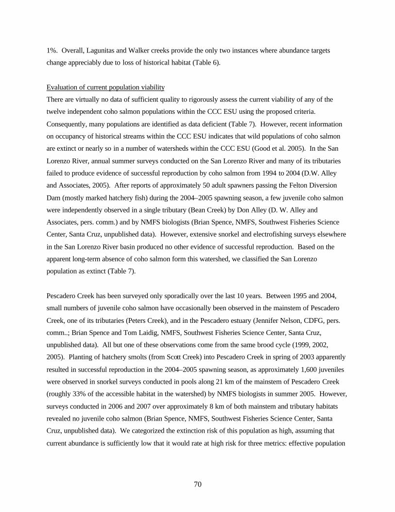
70

1%. Overall, Lagunitas and Walker creeks provide the only two instances where abundance targets

change appreciably due to loss of historical habitat (Table 6).

Evaluation of current population viability

There are virtually no data of sufficient quality to rigorously assess the current viability of any of the

twelve independent coho salmon populations within the CCC ESU using the proposed criteria.

Consequently, many populations are identified as data deficient (Table 7). However, recent information

on occupancy of historical streams within the CCC ESU indicates that wild populations of coho salmon

are extinct or nearly so in a number of watersheds within the CCC ESU (Good et al. 2005). In the San

Lorenzo River, annual summer surveys conducted on the San Lorenzo River and many of its tributaries

failed to produce evidence of successful reproduction by coho salmon from 1994 to 2004 (D.W. Alley

and Associates, 2005). After reports of approximately 50 adult spawners passing the Felton Diversion

Dam (mostly marked hatchery fish) during the 2004–2005 spawning season, a few juvenile coho salmon

were independently observed in a single tributary (Bean Creek) by Don Alley (D. W. Alley and

Associates, pers. comm.) and by NMFS biologists (Brian Spence, NMFS, Southwest Fisheries Science

Center, Santa Cruz, unpublished data). However, extensive snorkel and electrofishing surveys elsewhere

in the San Lorenzo River basin produced no other evidence of successful reproduction. Based on the

apparent long-term absence of coho salmon form this watershed, we classified the San Lorenzo

population as extinct (Table 7).

Pescadero Creek has been surveyed only sporadically over the last 10 years. Between 1995 and 2004,

small numbers of juvenile coho salmon have occasionally been observed in the mainstem of Pescadero

Creek, one of its tributaries (Peters Creek), and in the Pescadero estuary (Jennifer Nelson, CDFG, pers.

comm..; Brian Spence and Tom Laidig, NMFS, Southwest Fisheries Science Center, Santa Cruz,

unpublished data). All but one of these observations come from the same brood cycle (1999, 2002,

2005). Planting of hatchery smolts (from Scott Creek) into Pescadero Creek in spring of 2003 apparently

resulted in successful reproduction in the 2004–2005 spawning season, as approximately 1,600 juveniles

were observed in snorkel surveys conducted in pools along 21 km of the mainstem of Pescadero Creek

(roughly 33% of the accessible habitat in the watershed) by NMFS biologists in summer 2005. However,

surveys conducted in 2006 and 2007 over approximately 8 km of both mainstem and tributary habitats

revealed no juvenile coho salmon (Brian Spence, NMFS, Southwest Fisheries Science Center, Santa

Cruz, unpublished data). We categorized the extinction risk of this population as high, assuming that

current abundance is sufficiently low that it would rate at high risk for three metrics: effective population

Table 7. Current viability of CCC-Coho Salmon independent populations based on metrics outlined in Tables 1 and 4. na indicates data of sufficient quality to estimate the population metric are not available. In some cases, risk categories have been designated for populations where ancillary data strongly suggest populations are extinct or nearly so, despite the lack of quantitative estimates of any of the viability metrics. Metrics for which we believe ancillary data support the assigned risk category are denoted with asterisks. See text for justification of risk rankings.

PVA result

Effect. pop. size per

generation

Tot. pop. size per

generation Population decline Catastrophe Density Hatchery Risk Category

Population eN )(harmgN )(geoaN T C depD ssdD Ten Mile River na na na na na na na na na Data deficient Noyo River na na na na na na na na na* Moderate/High Big River na na na na na na na na na Data deficient Albion River na na na na na na na na na Data deficient Navarro River na na na na na na na na na Data deficient Garcia River na na* na* na* na na na* na* na High Gualala River na na* na* na* na na na* na* na High Russian River na na* na* na* na na na* na* na* High Walker Creek na na* na* na* na na na* na* na* Extinct? Lagunitas Creek na na na na na na na na na Data deficient* Pescadero Creek na na* na* na* na na na* na* na* High San Lorenzo River na na* na* na* na na na* na* na Extinct?

* See text for discussion of existing data for Lagunitas Creek.

71

72

size, population decline (mean annual spawner abundance), and spawner density (i.e., depensation risk;

Table 7). The planting of Scott Creek fish into Pescadero Creek potentially poses a genetic risk to any

remnant population that may still exist in the watershed, though these genetic risks may be trivial

compared with the existing demographic risks given the population’s apparent small size. Adult

abundance of one dependent population of coho salmon, Scott Creek, has also been estimated from weir

counts over the last four years (Sean Hayes, NMFS, Southwest Fisheries Science Center, Santa Cruz,

unpublished data). These estimates have averaged about 163 adults (range 6 to 329), though the 2005-

2006 and 2006-2007 estimates were only 49 and 6 fish, respectively, and preliminary reports from 2007-

2008 indicate very few returning adults. Hatchery fish accounted for about 34% of returning fish during

the past four years. This is believed to be the largest remaining population south of San Francisco Bay.

The most reliable set of population data for any independent population in the CCC ESU comes from

Lagunitas Creek, where spawner surveys have been conducted on a regular basis (flows permitting) since

1995. These surveys involve multiple visits to reaches representing a substantial portion of the available

spawning habitats (Ettlinger et al. 2005). Redd counts from these surveys appear to provide the most

consistent measure of abundance, as estimates of live spawners are likely biased high due to double -

counting of individuals on successive surveys. Over the last 12 years, an average of about 260 coho redds

(range 86-496) have been observed annually in the mainstem and upper tributaries of Lagunitas Creek.

Additionally, National Park Service surveys of Olema Creek (a tributary to Lagunitas Creek), where

maximum live/dead fish counts are recorded, indicate that a minimum of 86 fish have, on average,

spawned in Olema Creek over the last eight years. These data did not meet our minimum requirements

for application of viability metrics for several reasons. First, redd counts may lead to biased (both high

and low) estimates of spawner abundance for a number of reasons, such as failure of observers to detect

redds do to poor viewing conditions, redd superimposition, loss of redds due to scouring, individual

females constructing multiple redds, or unequal sex ratios. Consequently, they may provide only an

indicator of abundance24. Second, there is no information about spawner abundance in unsurveyed areas;

thus, obtaining a total population estimate from these data is not currently possible. And finally, the 10-

year time series does not yet meet the minimum data requirement of 4 generations for estimating effective

population size, population decline, or density criteria. Consequently, we categorized the population as

data deficient (Table 7). However, we note that with two additional years of data collection, additional

analysis of the relationship between redd counts and total spawner abundance, and analysis of the relative

24 Note that under the most favorable conditions (i.e., clear observation conditions throughout the spawning season, densities sufficiently low that superimposition is unlikely, and absence of scouring events), redd counts may prove to be an appropriate means for estimating adult spawner abundance; however, additional data are needed to establish a relationship between redd counts and total spawner abundance.

73

densities in surveyed versus unsurveyed reaches, these data could provide a reasonable basis for assessing

population viability. We also note that the existing data suggest that, if current patterns continue, and

assuming that one redd translates to approximately two spawning adults on average, the Lagunitas Creek

population might satisfy low-risk criteria for the effective population size criteria and perhaps the

population decline criteria as well. On the other hand, the population would likely be considered at

moderate risk based on the density criteria. Lagunitas Creek and its tributaries received plantings of

hatchery fish, primarily from the Noyo River but also from some out-of-ESU stocks, on numerous

occasions between 1960 and 1987 (Bjorkstedt et al. 2005). Analysis of DNA microsatellite data from

coho populations in California indicate some affinity between Lagunitas Creek and Noyo River coho

salmon (J. Carlos Garza, NMFS, Southwest Fisheries Science Center, Santa Cruz, unpublished data);

however, it is unclear whether this is the consequence of past hatchery plants or natural straying. Thus, it

is difficult to assess potential residual hatchery-related risk for Lagunitas Creek. To our knowledge, there

have been no recent plantings of hatchery fish into the Lagunitas watershed, suggesting that ongoing risks

due to hatchery operations are minimal.

Naturally occurring coho salmon have not been observed in Walker Creek in several decades, though this

stream was planted with 80 adult coho salmon (Olema Creek origin) from the Russian River captive

broodstock program in January of 2004, and fingerlings—confirmed through genetic analysis to be

primarily progeny of the planted adults—were observed in summer of 2004 (CDFG 2004; J. Carlos

Garza, NMFS, Southwest Fisheries Science Center, Santa Cruz, unpublished data). We categorized this

population as “extinct” based on the long-term absence of naturally spawning coho salmon from this

basin (Table 7).

In the Russian River basin, only one tributary (Green Valley Creek) has produced coho salmon annually

in recent years, with salmon observed only sporadically in a few other tributaries (Merritt Smith

Consulting 2003). Concerns over the decline of coho salmon in the Russian River basin have led to the

establishment of a captive broodstock program at the Warm Springs (Don Clausen) Hatchery. Based on

the sparse distribution (Good et al. 2005), the low apparent abundance, recent evidence of a genetic

bottleneck (Libby Gilbert-Hovarth et al., NMFS, Southwest Fisheries Science Center, Santa Cruz,

unpublished data, cited in Bjorkstedt et al. 2005), and the perceived need for intervention with a captive

broodstock program, we categorized the Russian River population as at high risk, assuming that it would

rank at high risk for at least four of five population metrics (Table 7)

74

Limited surveys in the Garcia and Gualala rivers have documented occasional occurrence of coho salmon

in the last 15 years, but the distribution of fish has been sparse in both river systems (Good et al. 2005).

Observations in the Gualala River may have resulted from planting of young-of-the-year coho salmon

from the Noyo River into the North Fork Gualala River in years 1995-1997 (Harris 2001). We

categorized both the Gualala River and Garcia River populations as at least at high risk of extinction, as it

is highly unlikely that either is sufficiently abundant to satisfy even the moderate risk criteria for effective

population size, population decline (i.e., annual abundance), and density (depensation) criteria (Table 7).

Status of populations along the Mendocino Coast is less certain, though monitoring of one independent

(Noyo River) and four dependent coho populations (Pudding Creek, Caspar Creek, Hare Creek, and Little

River) was initiated by the California Department of Fish and Game in 2000 and 2001 (Gallagher and

Wright 2007). Occupancy data suggest that populations in the Navarro, Albion, Big, Noyo, and Ten Mile

rivers continue to persist but that their distributions have been substantially reduced (Good et al. 2005).

In none of these cases are there sufficient population-level data to determine viability with any certainty;

thus, we classified four of these populations (Navarro, Albion, Big, and Ten Mile) populations as data

deficient (Table 7), though available occupancy data suggest that it is unlikely any are achieving the low-

risk density criteria threshold and therefore may be at least at moderate risk.

In the case of the Noyo River, counts of adult spawners are available from the Noyo Egg Collecting

Station on the South Fork Noyo River since 1962. These counts do not represent full counts (the station

was operated irregularly in most years, and only about one-third of the avaiable habitat in the basin is

located upstream of the ECS). Furthermore counts through 2005 are strongly influenced by hatchery

activities that occurred from the early 1960s to 2003, when the last releases of hatchery coho salmon

smolts were made. Counts from the mid 1990s to 2004 averaged about 620 fish; however, counts over

the last three years have been among the lowest on record, with 79 fish in 2005-2006, 59 fish in 2006-

2007, and even smaller numbers expected in 2007-2008. Estimates from Gallagher and Wright (2007)

made using a variety of methods suggest that total numbers of coho spawners above the ECS likely

exceed weir counts by 20% to 100%, depending on which estimator is used 25. During the last two

generations of hatchery operation, when all released hatchery yearlings were marked, returning hatchery

adults constituted an average of 59% and 45%, respectively. Based on these data, and the fact the roughly

one-third of the habitat in the Noyo River lies in the South Fork subbasin, we suspect that, even if

straying of South Fork Noyo hatchery fish into other subbasins is low, the total percentage of hatchery

25 A primary goal of this research is to evaluate a wide range of estimating procedures, ranging from live fish and carcass mark-recapture estimates, redd counts (raw and adjusted based on fish-per-redd estimates), and AUC estimates.

75

fish in the entire basin likely exceeded 15%. This conclusion assumes that density of natural spawners in

areas outside of the South Fork subbasin are not substantially higher than in the South Fork. Furthermore,

the long history of stocking during which practices were not consistent with current best management

practices (e.g., nonnative broodstock were occasionally used, and broodstock selection and mating

protocols generally did not follow modern BMPs) suggests the potential for residual genetic effects of

these operations. Thus, we classified Noyo River coho salmon as being at moderate/high risk due to past

hatchery influence (Table 7). Although direct plantings of coho salmon into the Ten Mile, Big, Navarro,

and Albion rivers do not currently occur, the potential exists for Noyo River hatchery fish to stray into

these watersheds. The degree to which they do so is not known.

For the four dependent populations on the Mendocino Coast that are currently monitored, Pudding Creek

has produced the largest numbers of spawning adults, averaging about 300 to 1200 fish, depending on

which estimator is used. For the remaining three populations, average numbers of returning adults is

estimated to be between 130 and 500 fish for Caspar Creek, 60-140 fish for Litte River, and 70-340 fish

for Hare Creek, depending on the estimator used (Gallagher and Wright 2007).

ESU Viability

Though quantitative data on the abundance of coho salmon in the CCC ESU are scarce and many

populations were described as data deficient (Table 7), ancillary data (primarily presence-absence data)

clearly indicate that coho salmon in this ESU fail to meet both the representation and

redundancy/connectivity criteria. The available data indicate that no populations meet low-risk criteria in

three of the identified diversity strata (Santa Cruz Mountains, Coastal, and Gualala Point-Navarro Point),

and that coho salmon are no longer present in an any of the San Francisco Bay dependent populations

(indicating that either neighboring populations are not producing migrants in sufficient number to

maintain these populations or the available habitat is incapable of supporting any migrants that do enter

these systems). Status of populations along the Mendocino Coast is highly uncertain (all populations

were categorized as data deficient), though we believe it is unlikely that any of these populations

approach viable levels.

Connectivity among populations within and among diversity strata is a significant concern. Within the

Santa Cruz Mountains stratum, the two identified functionally independent populations appear extinct

(San Lorenzo River) or nearly so (Pescadero Creek). Dependent coho salmon populations still persist in

three watersheds near the geographic center of the stratum, but only the Scott Creek population, which is

supported by ongoing hatchery activities, has regularly produced spawners in all three brood lineages in

76

recent years, and returns in the last two spawning seasons have been extremely poor. Both the Waddell

Creek and Gazos Creek populations appear to have lost two year classes (Smith 2006; B. Spence, NMFS

Santa Cruz, unpublished data). Coho salmon are occasionally observed in other watersheds (e.g., San

Vicente, San Gregorio, and Laguna creeks), but these fish are likely the product of strays from either

Scott Creek or hatchery fish that have been planted in area streams. Consequently, there are substantial

portions of the stratum that have few or no coho salmon, and the nearest extant population to the north is

Redwood Creek in Marin County, a dependent population some 100 km to the north. Likewise, in the

Coastal stratum, coho salmon persist in significant numbers only in Lagunitas Creek, with a few coho

found in the Russian River, as well as Redwood Creek to the south. To the north, in the Navarro Point-

Gualala Point stratum, coho salmon appear scarce or extinct in all watersheds with the exception of the

Navarro River. As the Lagunitas Creek and Navarro River populations are separated by an expanse of

almost 160 km of coastline with almost no coho salmon, interactions among these populations may be

minimal. Connectivity is currently less of a concern in the Lost Coast-Navarro Point stratum, as both

independent and dependent populations of coho salmon still persist from Big Salmon Creek to the Ten

Mile River (Good et al. 2005). It is unclear, however, how much recent distribution patterns have been

influenced by hatchery operations within the Noyo River basin. The status of dependent populations to

north of the Ten Mile River is poorly known, but it is possible that the Mattole River, in the SONCC

ESU, is the nearest extant population that supports coho salmon on an annual basis. Coho salmon were

observed in two consecutive years in the South Fork of Usal Creek (W. Jones, CDFG retired, personal

observations), but it is uncertain whether coho salmon occur in all three brood years.

In summary, the lack of demonstrably viable populations (or the lack of data from which to assess

viability) in any of the strata, the lack of redundancy in viable populations in any of the strata, and the

substantial gaps in the distribution of coho salmon throughout the CCC ESU strongly indicate that this

ESU is currently in danger of extinction. Our conclusion is consistent with recently published status

reviews prepared by the National Marine Fisheries Service (Good et al. 2005) and the California

Department of Fish and Game (CDFG 2002).

4.2 California Coastal Chinook Salmon


Summary of density-based criteria

The NCCC TRT (Bjorkstedt et al. 2005) proposed that the CC-Chinook ESU historically comprised

fifteen independent populations of fall-run Chinook salmon (10 functionally independent and five

77

potentially independent) and six independent populations of spring-run Chinook salmon (all functionally

independent26). However, the TRT also noted that, due to the lack of historical data on Chinook salmon

abundance within the ESU, the hypothesized population structure is subject to substantial uncertainty.

Contributing to this uncertainty are 1) an incomplete understanding of histor ical habitat connectivity and

resulting spatial structure of various breeding groups, particularly in the larger watersheds such as the Eel

and Russian rivers, where plausible structures range from one or two large populations to multiple smaller

populations occupying different subwatersheds; and 2) the scarcity of historical evidence of Chinook

salmon in watersheds in Mendocino and Sonoma counties, which leads to some uncertainty about

whether these populations functioned as independent units27. In the absence of definitive information,

population designations were based primarily on predictions from our IP model and connectivity-viability

analysis (Bjorkstedt et al. 2005). Table 8 presents proposed density-based criteria for these populations

and the estimated population abundances (rounded to the nearest 100 spawners) that would result if

density criteria were met under both historical (pre-dam) and current (post-dam) conditions. As before,

high-risk abundance values indicate thresholds below which depensation is likely under both historical

and current conditions. Low-risk estimates based on historically accessible habitat provide preliminary

abundance targets that, if consistently exceeded, we believe would lead to a high probability of

persistence over a 100-year time frame and the population fulfilling its historical role in ESU viability.

Comparison of historical versus current IPkm indicates that Chinook salmon in two populations, the

Upper Eel River and Russian River populations, have lost access to appreciable amounts of habitat due to

impassible dams. Scott Dam in the upper Eel River results in an estimated 11% loss of potential habitat.

In the Russian River, a 15% reduction in potential habitat is attributed to dams, with Warm Springs and

Coyote dams accounting for most of those losses.

26 Evidence of historical occurrence is lacking for three of the six proposed spring-run populations (Redwood Creek, Van Duzen River, and the Upper Eel River). These populations were assumed to have existed based on environmental similarities between the upper portions of these watersheds and those believed to have supported spring Chinook, as well as by the historical occurrence of summer steelhead, which share similar oversummering habitat requirements (Bjorkstedt et al. 2005). 27 The paucity of historical evidence of Chinook salmon in rivers of Mendocino and northern Sonoma counties may in part reflect the fact that by the late 1800s, substantial alteration to streams had already taken place as a result of logging activities. These activities included not only the harvest of redwoods forests, but also the transport of logs downstream through use of splash dams and log drives (see e.g., Jackson 1991; Downie et al. 2006). These activities undoubtedly had tremendous impact on habitat suitability for Chinook salmon, which spawn primarily in mainstems and larger tributaries where log drives occurred repeatedly.

78

Evaluation of current population viability

Fall-run populations

Currently available data are insufficient to rigorously evaluate the current viability of any of the fifteen

putative independent populations of fall-run Chinook salmon in the CC-ESU using the proposed criteria.

There are no population-level abundance estimates for any populations within the ESU that meet the

minimum requirements for application of viability criteria outlined in Table 4. For certain populations,

ancillary data are available, but in few cases do they allow for risk categorization. These data are

reviewed below.

In the Redwood Creek watershed, spawner surveys have been conducted over approximately 17 km of

Prairie Creek and its tributaries since the 1998-1999 spawning season. Population estimates for the

surveyed reaches have averaged 342 (range 106-531) over six years (Walt Duffy and Steve Gough,

Humboldt State University, unpublished data). However, there is no information on Chinook abundance

in the mainstem of Redwood Creek or its other tributaries, which have been substantially more influenced

by land-use practices. Spawner surveys have been conducted annually since the early 1980s on a 2 mi

reach of Canon Creek, tributary to the Mad River (PFMC 2007). Maximum live-dead counts (including

jacks) have ranged from 0 to 514 (mean = 107); however, because these surveys cover only a small

portion of the available habitat and are variable from year to year in frequency, they cannot be used to

derive population-level estimates of abundance or trends. Data from spawner surveys in index reaches of

Tomki and Sprowl creeks in the upper Eel River are also available since the late 1970s (PFMC 2007). At

Tomki Creek, maximum live-dead counts have ranged from 0 to 2,187 (mean = 244), though the average

over the last twelve years has declined to 144 spawners. For Sprowl Creek, maximum live-dead counts

over 4.5 mi of stream have ranged from 3 to 3,666 (mean = 741) since the late 1970s; however, over the

last twelve years, counts have averaged only 68 spawners. In both these case, the estimates are most

appropriately viewed as “floors” of abundance, and inconsistencies among years preclude their use as a

reliable indicator of trend. Chinook salmon counts are also made at the Van Arsdale Fish Station in

the upper mainstem Eel River, but these are similarly inappropriate for estimating population-level

abundance (Good et al. 2005). A weir on Freshwater Creek has provided a reasonable census of adult

Chinook counts for the period 1994-2004 (Good et al. 2005), with abundance averaging about 54 fish

from 1994 to 2003. However, because Freshwater Creek represents only one of four Chinook-bearing

streams within the putative Humboldt Bay independent population, we deem the data insufficient for

assessing status at the population level. For both Bear River and Little River populations, we know of no

current datasets of adult abundance. For these reasons, we categorized the Redwood Creek, Mad River,

Humboldt Bay, Eel River, Little River, and Bear River populations as data deficient (Table 9).

Table 8. Projected population abundances (Na) of CC-Chinook Salmon independent populations corresponding to a high-risk (depensation) threshold of 1 spawner/IPkm and low-risk (spatial structure/diversity=SSD) thresholds based on application of spawner density criteria (see Figure 5). Values listed under “historical” represent criteria applied to the historical landscape in the absence of dams that block access to anadromous fish. Values listed under “current” exclude areas upstream from impassible dams.

High Risk Low Risk Historical Current Historical SSD Current SSD Historical Current IPkm Depens. Depens. Density Density

Population IPkm IPkm Lost Na Na Spawner/IPkm Na Spawner/IPkm Na Fall-run populations Redwood Creek (H) 116.1 116.1 0% 116 116 29.3 3400 29.3 3400 Little River (H) 18.6 18.6 0% 19 19 40.0 700 40.0 700 Mad River 94.0 94.0 0% 94 94 31.8 3000 31.8 3000 Humboldt Bay 76.7 76.7 0% 77 77 33.7 2600 33.7 2600 Lower Eel River 514.9 514.9 0% 515 515 20.0 10300 20.0 10300 Upper Eel River 555.9 495.3 11% 556 495 20.0 11100 20.0 9900 Bear River 39.4 39.4 0% 39 39 37.8 1500 37.8 1500 Mattole River 177.5 177.5 0% 178 178 22.5 4000 22.5 4000 Ten Mile River 67.2 67.2 0% 67 67 34.8 2300 34.8 2300 Noyo River 62.2 62.2 0% 62 62 35.3 2200 35.3 2200 Big River 104.3 104.3 0% 104 104 30.6 3200 30.6 3200 Navarro River 131.5 131.5 0% 131 131 27.6 3600 27.6 3600 Garcia River 56.2 56.2 0% 56 56 36.0 2000 36.0 2000 Gualala River 175.6 175.6 0% 176 176 22.7 4000 22.7 4000 Russian River 584.2 496.4 15% 584 496 20.0 11700 20.0 9900 Spring-run populations (Redwood Creek (H)) 116.1 116.1 0% * * * * * * Mad River 94.0 94.0 0% * * * * * * (Van Duzen River) 109.5 109.5 0% * * * * * * North Fk Eel River 76.8 76.8 0% * * * * * * Middle Fk Eel River 188.5 188.5 0% * * * * * * Upper Eel River 89.1 29.3 67% * * * * * * * Density criteria are not applied to spring-run Chinook salmon; availability of oversummering pools for adults are more likely to limit abundance than IP-based predictions of spawning habitat. IP values for fall Chinook are presented for spring Chinook populations soley to provide a rough index of the percentage of habitat that lies upstream of dams.

79

80

The Mattole Salmon Group has conducted spawner and redd surveys on the Mattole River and its

tributaries since 1994. Local experts have used these surveys and ancillary data to develop a rough

“index” estimates of spawner escapement to the Mattole River; however, sampling intensity and spatial

extent of surveys have varied from year to year, which makes them unsuitable for rigorous estimates of

abundance or trend (MSG 2005; Good et al. 2005). The redd counts, which provide the best indicator of

escapement, have ranged from 27 to 88 during the ten years of surveys. Based on the these data, we

conclude that the population is likely at elevated risk of extinction but are unable to assess whether the

population is at moderate or high risk of extinction (Table 9).

The status of Chinook salmon in coastal watersheds of the Mendocino and northern Sonoma counties,

from the Ten Mile River to the Gualala River, is highly uncertain. To our knowledge, recent documented

occurrences are limited to observations of a few adult spawners in the Ten Mile River during the mid-

1990s (Maahs 1996) 28 and collection of juvenile Chinook salmon in downstream migrant traps located on

the Noyo River (Gallagher 2001). Additionally, adult Chinook salmon are occasionally observed in the

Noyo River during spawner surveys or at the Noyo Egg Collecting Station, and a single adult was

observed in the Navarro River in the 2006–2007 spawning season (Scott Harris, California Department of

Fish and Game, Willits, pers. comm.). Bell (2003) reports that Chinook salmon in the Garcia River are

extinct. We know of no recent documented occurrences of Chinook salmon in the Big River or Gualala

River basins, though anecdotal reports from fisherman suggest that Chinook salmon occasionally visit

these watersheds. Based on this limited information, the TRT suspects that these six independent

populations of Chinook salmon from Ten Mile River to the Gualala River are at least at high risk of

extinction and in some cases may be extinct (Table 9). We chose to categorize them as high-risk (rather

than extinct) because of the lack of spawner surveys conducted on mainstem portions of these rivers,

where spawning by Chinook is most likely to occur.

Spawner surveys were initiated in the Russian River in 2000, and video monitoring at two fish ladders

located at the Mirabel Inflatable Dam has provided counts of Chinook adults since 2002. Although the

time series does not meet our minimum criteria for duration (four generations) and does not represent a

full count (some adults spawn lower in the basin, and the dam is typically deflated in December when

flows get too high), the data do suggest the Chinook run has been substantial in recent years. Chinook

counts have averaged more than 3,600 fish (range 1,383 to 6,103) over the last six years (Cook 2005,

28 Maahs (1996) estimated the total number of adult spawners in the Ten Mile River to be fewer than 10 in the 1995-1996 spawning season.

Table 9. Current viability of CC-Chinook salmon independent populations based on metrics outlined in Tables 1 and 4. na indicates data of sufficient quality to estimate the population metric are not available. In some cases, risk categories have been designated for populations where ancillary data strongly suggest populations are extinct or nearly so, despite the lack of quantitative estimates of any of the viability metrics. Metrics for which we believe ancillary data support the assigned risk category are denoted with asterisks. See text for justification of risk rankings.

Population Name PVA result


generation

Tot. pop. size per

generation Population decline Catastrophe Density Hatchery Risk Category

eN )(harmgN )(geoaN T C depD ssdD Fall-run populations Redwood Creek (H) na na na na na na na na na Data deficient Little River (H) na na na na na na na na na Data deficient Mad River na na na na na na na na na Data deficient Humboldt Bay na na na na na na na na na Data deficient Lower Eel River na na na na na na na na na Data deficient Upper Eel River na na na na na na na na na Data deficient Bear River na na na na na na na na na Data deficient Mattole River na na* na* na* na na na na* na Moderate/High Ten Mile River na na* na* na* na na na na* na High Noyo River na na* na* na* na na na na* na High Big River na na* na* na* na na na na* na High Navarro River na na* na* na* na na na na* na High Garcia River na na* na* na* na na na na* na High Gualala River na na* na* na* na na na na* na High Russian River na na na na na na na na na Data deficient Spring-run populations (Redwood Creek (H)) - - - - - - - - - Extinct Mad River [5] - - - - - - - - - Extinct (Van Duzen River) - - - - - - - - - Extinct North Fk Eel River - - - - - - - - - Extinct Middle Fk Eel River - - - - - - - - - Extinct Upper Eel River - - - - - - - - - Extinct

81

82

2006). Were such patterns to continue, the population would likely meet most low-risk viability

thresholds for all criteria except perhaps the density criterion.

Spring-run populations

All six spring-run independent populations of Chinook salmon in the CC-Chinook ESU are believed

extinct.

ESU Viability

The complete lack of population-level information on the distribution and abundance of Chinook salmon

throughout the CC-Chinook salmon ESU precludes application of the ESU-level viability criteria (Table

9). Most available information consists of spawning surveys in index reaches, for which the limited and

non-random spatial extent, coupled with variation in survey frequency, render the data inappropriate for

assessing population abundance or trend. Though more rigorous sampling has been conducted on Prairie

Creek (tributary to Redwood Creek) and Freshwater Creek, in both cases the estimates represent only a

portion the total population. Monitoring of spawning Chinook salmon in the Russian River has improved

considerably in the last 5–6 years; however, this time series is not sufficiently long to assess trends.

With data limitations in mind, we identify several areas of significant concern as they relate to viability of

the CC-Chinook salmon ESU. The current distribution of extant populations includes several watersheds

in Humboldt County including Redwood Creek, Little River, Mad River, Humboldt Bay, Eel River (with

two populations), Bear River, and Mattole River, as well as some smaller watersheds such as Maple

Creek, Jacoby Creek, and Salmon Creek. However, the lack of population data precludes us from

determining whether there are viable independent populations of fall run Chinook in the North Coastal or

North Mountain Interior strata. Additionally, spring Chinook salmon within the ESU are thought to be

extinct, indicating loss of diversity within the ESU. Currently, there are no known extant and persistent

populations between the Mattole River in Humoldt County and the Russian River in Sonoma County, a

distance of approximately 200 km. Consequently, there appears to be no representation of the North-

Central Coastal stratum, and connectivity between the Mattole River population and the Russian River

population is likely substantially reduced from historical patterns. Because of the lack of population data,

viability of the Russian River population is uncertain. However, even if the Russian River population is

eventually deemed viable, the lack of other viable populations within the Central Coastal stratum places

this stratum at greater risk due to catastrophic risks, such as disturbances to the mainstem Russian River

where most spawning is believed to occur.

83

In summary, the lack of data from which to assess viability of extant populations in the northern part of

the ESU, the apparent lack of extant populations, with the exception of the Russian River, in the southern

half of the ESU, the loss of important life-history diversity (i.e. spring-run populations), and the

substantial gaps in the distribution of Chinook salmon throughout the CC ESU strongly indicate that this

ESU fails to meet low-risk criteria and is therefore at elevated risk of extinction. Our conclusion is

qualitatively consistent with recently published NMFS status reviews (NMFS 1999; Good et al. 2005).

4.3 Northern California Steelhead



Bjorkstedt et al. (2005) proposed that the NC-Steelhead ESU historically consisted of 41 independent

populations of winter-run steelhead (19 functionally independent and 22 potentially independent29), and

as many as 10 populations of summer steelhead (all functionally independent). Table 10 summarizes

proposed density-based criteria for these populations and the projected population abundances (rounded

to the nearest 100 spawners) that would result if density criteria were met under both historical (pre-dam)

and current (post-dam) conditions. High-risk abundance values indicate thresholds below which

depensation is likely, and low-risk abundance values for historical conditions represent preliminary

abundance targets that, if consistently exceeded, would likely lead to a high probability of persistence

over a 100-year time frame and result in a population likely fulfilling its role in ESU viability.

Comparison of historical versus currently available IPkm indicates that two steelhead populations, the

Mad River population and the Upper Mainstem Eel River population, have lost substantial habitat due to

dams. In the Mad River, an estimated 36% of potential steelhead habitat lies above Ruth Dam, though a

partial barrier well downstream of Ruth Dam may limit use of the upper watershed by steelhead in some

years. For the upper mainstem Eel River, the Scott Dam blocks access to more than 99% of available

habitat upstream of Soda Creek. The remaining 2.7 IPkm of habitat is insufficient to support a viable

population, though the IP model predicts that this population once may have joined the South Fork Eel,

North Fork Eel, Middle Fork Eel, and Van Duzen populations as the largest populations in the watershed.

Outlet Creek has dams that block access to about 7% of historical potential habitat. Habitat loss

attributable to dams is 1% or less for all other populations (Table 10).

29 The TRT has since added one more potentially independent population, Soda Creek in the upper Eel River. See Appendix A.

Table 10. Projected population abundances (Na) of NC-Steelhead independent populations corresponding to a high-risk (depensation) threshold of 1 spawner/IPkm and low-risk (spatial structure/diversity=SSD) thresholds based on application of spawner density criteria (see Figure 5). Values listed under “historical” represent criteria applied to the historical landscape in the absence of dams that block access to anadromous fish. Values listed under “current” exclude areas upstream from impassible dams. The IP -bias index is a qualitve measure of possible hydrologic bias in the IP model that could potentially lead to overprediction of historical habitat for juvenile coho salmon (Bjorkstedt et al. 2005).

High Risk Low Risk Historical Current Historical SSD Current SSD Historical Current IPkm IP bias Depens. Depens. Density Density Population IPkm IPkm lost index Na Na Spawner/IPkm Na Spawner/IPkm Na Redwood Creek (H) 301.1 301.1 0% low 301 301 20.0 6000 20.0 6000 Maple Creek/Big Lagoon 94.7 94.7 0% low 95 95 29.1 2800 29.1 2800 Little River (H) 76.2 76.2 0% low 76 76 31.6 2400 31.6 2400 Mad River 553.2 351.8 36% low 553 352 20.0 11200 20.0 7000 Humboldt Bay 283.0 283.0 0% low 283 283 20.0 5700 20.0 5700 Eel River - Full Price Creek 20.6 20.6 0% low 21 21 39.4 800 39.4 800 Van Duzen River 363.8 363.8 0% low 364 364 20.0 7300 20.0 7300 Larabee Creek 101.0 101.0 0% low 101 101 28.2 2800 28.2 2800 South Fork Eel River 1182.1 1182.1 0% low 1182 1182 20.0 23600 20.0 23600 Dobbyn Creek 52.5 52.5 0% low 52 52 34.9 1800 34.9 1800 Jewett Creek 18.2 18.2 0% low 18 18 39.7 700 39.7 700 Pipe Creek 18.2 18.2 0% low 18 18 39.7 700 39.7 700 Kekawaka Creek 35.3 35.3 0% low 35 35 37.3 1300 37.3 1300 Chamise Creek 38.0 38.0 0% low 38 38 37.0 1400 37.0 1400 North Fork Eel River 372.8 372.8 0% low 373 373 20.0 7500 20.0 7500 Bell Springs Creek 18.5 18.5 0% moderate 19 19 39.6 700 39.6 700 Woodman Creek 39.4 39.4 0% moderate 39 39 36.7 1400 36.7 1400 Outlet Creek 313.8 292.9 7% moderate 314 293 20.0 6300 20.0 5900 Tomki Creek 131.7 131.7 0% moderate 132 132 23.9 3200 23.9 3200 Middle Fork Eel River 584.3 581.4 0% low 584 581 20.0 11700 20.0 11600 Bucknell Creek 21.1 21.1 0% moderate 21 21 39.3 800 39.3 800 Soda Creek 17.6 17.6 0% moderate 18 18 39.8 700 39.8 700 Upper Mainstem Eel River 387.3 2.7 99% moderate 387 3 20.0 7700 - - Bear River 114.8 114.8 0% low 116 116 26.1 3000 26.1 3000 Mattole River 613.9 613.9 0% low 614 614 20.0 12300 20.0 12300 Usal Creek 19.0 19.0 0% low 19 19 39.6 700 39.6 700 Cottaneva Creek 26.1 26.1 0% low 26 26 38.6 1000 38.6 1000

84

Table 10. (continued) High Risk Low Risk Historical Current Historical SSD Current SSD Historical Current IP bias Depens. Depens. Density Density Population IPkm IPkm IP-lost index Na Na Spawner/IPkm Na Spawner/IPkm Na Wages Creek 19.9 19.9 0% low 20 20 39.5 800 39.5 800 Ten Mile River 204.7 204.7 0% moderate 205 205 20.0 4100 20.0 4100 Pudding Creek 32.0 32.0 0% moderate 32 32 37.8 1200 37.8 1200 Noyo River 199.1 196.7 1% moderate 199 197 20.0 4000 20.0 3900 Hare Creek 18.1 18.1 0% moderate 18 18 39.7 700 39.7 700 Caspar Creek 16.0 16.0 0% moderate 16 16 40.0 600 40.0 600 Russian Gulch (Me) 19.2 19.2 0% moderate 19 19 39.6 800 39.6 800 Big River 316.6 312.9 1% high 317 313 20.0 6300 20.0 6300 Albion River 77.1 77.1 0% high 77 77 31.5 2400 31.5 2400 Big Salmon Creek 24.8 24.8 0% high 25 25 38.8 1000 38.8 1000 Navarro River 458.2 457.9 0% high 458 458 20.0 9200 20.0 9200 Elk Creek 24.3 24.3 0% high 24 24 38.9 900 38.9 900 Brush Creek 28.3 28.3 0% high 28 28 38.3 1100 38.3 1100 Garcia River 169.0 169.0 0% high 169 169 20.0 3400 20.0 3400 Gualala River 478.0 476.3 0% high 478 476 20.0 9600 20.0 9500

85

86

Evaluation of current viability

Winter-run populations

Currently available data are insufficient to rigorously evaluate the current viability of any of the 42

independent populations of winter steelhead in the NC-steelhead DPS using our viability criteria. Perhaps

the best available time series of adult spawner abundance comes from Freshwater Creek, one of several

streams that collectively make up the Humboldt Bay independent population. The Humboldt Fish Action

Council has operated a weir on Freshwater Creek since the 1994–1995 season, and annual adult steelhead

counts during this period have averaged about 73 adults (Seth Ricker, CDFG, Arcata, unpublished data).

Within the last four years, mark-recapture studies have been conducted to derive escapements estimates

for Freshwater Creek, and these have suggested that the weir has sampled from 38 to 74 percent of the

upstream migrants. However, because the time series of escapement estimates of insufficient length to

meet our criteria, and because the data represent only a portion of the Humboldt Bay population, which

also includes Jacoby Creek, Elk River, and Salmon Creek (among others) we categorize the Humboldt

population as data deficient (Table 11).

The Mattole Salmon Group conducts spawner surveys on the Mattole River; however, these surveys

target Chinook and coho salmon, collecting only incidental data on winter steelhead (MSG 2005). On the

Mendocino Coast, CDFG began monitoring steelhead in four independent populations (Pudding Creek,

Noyo River, Hare Creek and Caspar Creek), as well as one dependent population (Little River) in 2000

and 2001. Estimated ranges of abundance for these streams over a three-to-six year period are as follows:

Noyo River 186-364, Pudding Creek 76-265, Hare Creek 52-99, Caspar Creek 26-145, and Little River

16-34, (Gallagher and Wright 2007) 30. Although the time series of abundances are not sufficiently long to

meet our criteria, in all cases, the recent abundance ranges fall well below low-risk targets for spawner

density (Table 10), suggesting that if the current patterns hold for two to three more generations, all of

these populations would be considered at least at moderate risk. Thus, we classified these populations as

such.

Steelhead spawner surveys on the Gualala River were initiated in 2001 (DeHaven 2005). These surveys

are conducted on approximately 29 km of habitat in the Wheatfield Fork of the Gualala River and thus do

not allow for estimation of total population abundance in the Gualala River basin. Consequently, we

categorize these populations as data deficient as well (Table 11).

30 Estimates based on live fish capture-recapture estimates (where available) or fish per redd estimates, per the recommendation of Sean Gallagher, CDFG, pers. comm.

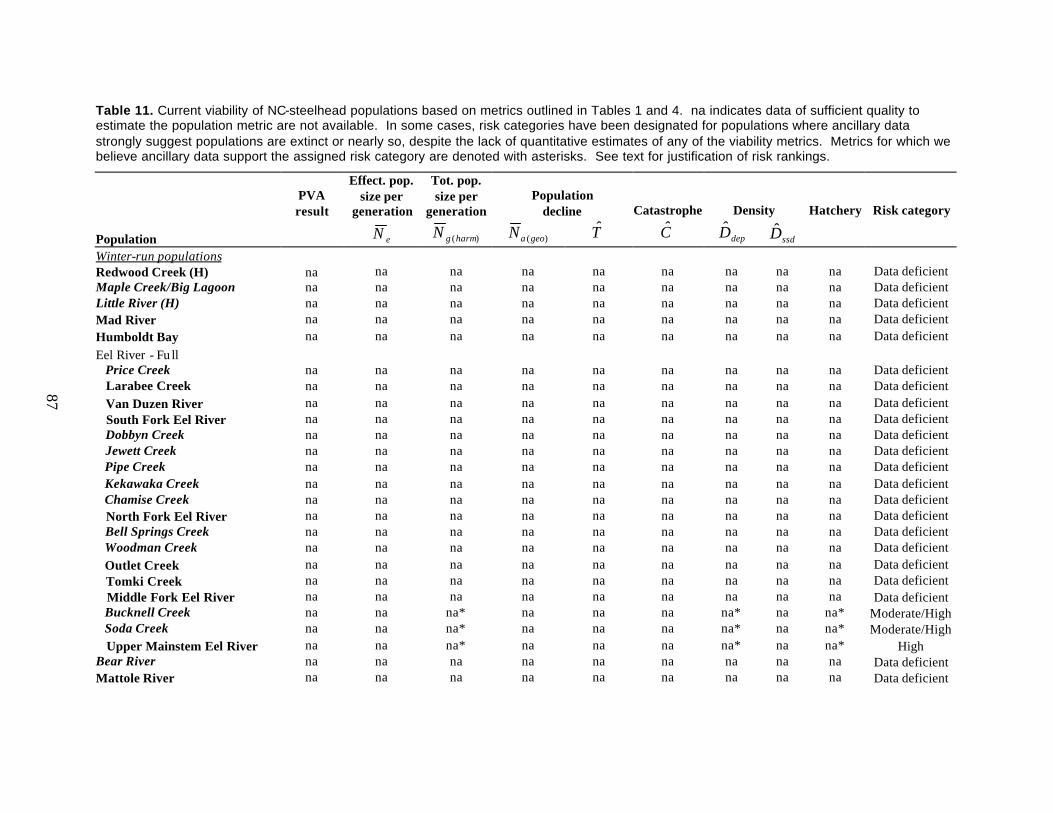
Table 11. Current viability of NC-steelhead populations based on metrics outlined in Tables 1 and 4. na indicates data of sufficient quality to estimate the population metric are not available. In some cases, risk categories have been designated for populations where ancillary data strongly suggest populations are extinct or nearly so, despite the lack of quantitative estimates of any of the viability metrics. Metrics for which we believe ancillary data support the assigned risk category are denoted with asterisks. See text for justification of risk rankings.

PVA result


generation

Tot. pop. size per

generation Population

decline Catastrophe Density Hatchery Risk category

Population eN )(harmgN )(geoaN T C depD ssdD Winter-run populations Redwood Creek (H) na na na na na na na na na Data deficient Maple Creek/Big Lagoon na na na na na na na na na Data deficient Little River (H) na na na na na na na na na Data deficient Mad River na na na na na na na na na Data deficient Humboldt Bay na na na na na na na na na Data deficient Eel River - Fu ll Price Creek na na na na na na na na na Data deficient Larabee Creek na na na na na na na na na Data deficient Van Duzen River na na na na na na na na na Data deficient South Fork Eel River na na na na na na na na na Data deficient Dobbyn Creek na na na na na na na na na Data deficient Jewett Creek na na na na na na na na na Data deficient Pipe Creek na na na na na na na na na Data deficient Kekawaka Creek na na na na na na na na na Data deficient Chamise Creek na na na na na na na na na Data deficient North Fork Eel River na na na na na na na na na Data deficient Bell Springs Creek na na na na na na na na na Data deficient Woodman Creek na na na na na na na na na Data deficient Outlet Creek na na na na na na na na na Data deficient Tomki Creek na na na na na na na na na Data deficient Middle Fork Eel River na na na na na na na na na Data deficient Bucknell Creek na na na* na na na na* na na* Moderate/High Soda Creek na na na* na na na na* na na* Moderate/High Upper Mainstem Eel River na na na* na na na na* na na* High Bear River na na na na na na na na na Data deficient Mattole River na na na na na na na na na Data deficient

87

Table 11. (continued)

PVA result


generation

Tot. pop. size per

generation Population

decline Catastrophe Density Hatchery Risk Category

Population

eN )(harmgN )(geoaN T C depD ssdD

Usal Creek na na na na na na na na na Data deficient Cottaneva Creek na na na na na na na na na Data deficient Wages Creek na na na na na na na na na Data deficient Ten Mile River na na na na na na na na na Data deficient Pudding Creek na na na na na na na na* na Moderate Noyo River na na na na na na na na* na Moderate Hare Creek na na na na na na na na* na Moderate Caspar Creek na na na na na na na na* na Moderate Russian Gulch (Me) na na na na na na na na na Data deficient Big River na na na na na na na na na Data deficient Albion River na na na na na na na na na Data deficient Big Salmon Creek na na na na na na na na na Data deficient Navarro River na na na na na na na na na Data deficient Elk Creek na na na na na na na na na Data deficient Brush Creek na na na na na na na na na Data deficient Garcia River na na na na na na na na na Data deficient Gualala River na na na na na na na na na Data defic ient Summer-run populations Redwood Creek (H) na na 18 (high) 4.6 (high) -0.04 (high) 0.86 (mod) - - low High Mad River na na* na* na* na* na - - na Moderate Van Duzen River na na na na na na - - na Data deficient Larabee Creek na na na na na na - - na Data deficient South Fork Eel River na na na na na na - - na Data deficient North Fork Eel River na na na na na na - - na Data deficient (Up. Mid. Mainstem Eel R) na na na na na na - - na Data deficient Middle Fk Eel River na na 2333 (mod) 569 (low) -0.01 (mod) 0.52 (low) - - low Moderate (Upper Mainstem Eel R) na na na na na na - - na Data deficient Mattole River na na* na* na* na* na - - na High

88

89

The only other time series of abundance for winter-run steelhead populations within this ESU is the count

of hatchery and wild steelhead at Van Arsdale Fish Station on the upper Eel River. The counts of wild

fish represent a composite of several delineated populations: Bucknell Creek, Soda Creek, the Upper

Mainstem Eel River (the mainstem and tributaries upstream of Soda Creek), and various dependent

populations between Van Arsdale station and Bucknell Creek. As such, the data cannot be used to

evaluate any of these populations directly. However, annual counts of wild fish have averaged just under

200 fish over the last 11 years (Grass 2007). Thus, even if all fish were concentrated in Bucknell Creek,

Soda Creek, or the Upper Mainstem Eel River, which does not appear to be the case (Scott Harris, CDFG,

Willits, CA , pers. comm.), the abundances still would not be sufficient to meet low risk criteria (or

moderate risk, in the case of the upper mainsteam Eel River) for effective population size or spawner

density. Additionally, in eight of the last 11 years, there has been a substantial hatchery influence, with

hatchery fish outnumbering wild fish by almost 10 to 1 during those years (Grass 1997-2007). For these

reasons, we conclude that the Bucknell Creek, Soda Creek, and Upper Mainstem Eel River populations of

winter steelhead are at least at moderate risk and probably at high risk of extinction.

Summer-run populations

Data on the abundance of summer-run steelhead are more readily available due to the fact that adults

congregate in “resting pools” during the summer and can be observed when water is relatively clear.

Currently, there are four ongoing efforts to estimate populations of summer steelhead in rivers within the

NC-steelhead DPS: Redwood Creek, Mad River, Middle Fork Eel River, and Mattole River.

Summer dive surveys covering almost the entire mainstem of Redwood Creek have been conducted

annually since 1981. There is some question about the reliability of some of the early counts, and it is

unclear about how much summer steelhead may use tributaries to Redwood Creek for holding. However,

recent abundance estimates in the mainstem clearly indicate a population that is at very high risk of

extinction. Mean adult abundance has averaged only 6 fish over the past four generations, and although

the recent trend over the last four generations has been just slightly negative (T = -0.021), the overall

trend for the entire period of record has continued downward (T = -0.046)(Dave Anderson, Redwood

National and State Parks, Crescent City, unpublished data). Effective population size is estimated to be at

just 3.6 fish. Consequently, we conclude this population is at high risk of extinction (Table 11).

Diver counts of summer steelhead have been conducted on portions of the Mad River since 1982. From

1982 to 2002, the Forest Service conducted surveys on the reach from Ruth Dam to Deer Creek; however,

that effort was terminated due to budget constraints. Since 1994, Green Diamond Resource Company

90

(formerly Simpson Timber Company) and the California Department of Fish and Game have surveyed the

reaches from Deer Creek to Mad River Hatchery, and from the hatchery to Cadle Hole, respectively.

Although the data do not meet the minimum requirements to formally assess viability using our criteria,

they do provide some indications of population status. For the period from 1994 to 2002, the period

where all three reaches were surveyed, geometric mean abundance was about 250 fish and the population

has declined throughout the period. Hatchery fish constituted about 2% for the two generations covered

during this period (Matt House, Green Diamond Resource Company, Korbel, unpublished data; Andrew

Bundschuh, US. Forest Service, Six Rivers National Forest, Eureka, unpublished data). Based on these

data, we conclude that the population is at least at moderate risk of extinction (Table 11).

The Middle Fork Eel River constitutes perhaps the only population within the entire recovery domain

where the existing time series of adult abundance estimates meet requirements outlined in Table 4.

Summer surveys of adults in summer resting pools have provided a reasonable census of the adult

population size dating back to the 1960s. Counts have ranged from 198 to 1601 during that period (Jones

1980, 1992; Jones et al. 1980; and Scott Harris, California Department of Fish and Game, Willits,

unpublished data). Calculation of extinction risk metrics, shown in Table 11, indicates that the population

currently ranks at low risk of extinction according to the population decline criteria (but only marginally

so) and for the catastrophe criteria. For the last four generations, the geometric mean abundance has been

over the 500 fish threshold, but only by a small amount, and the trend suggests a slight decline in

abundance (T = -0.010). However, over the entire period of record, the downward trend is more

pronounced (T = -0.025). Continued decline at this rate would have it approaching an Na of less than 500

within two generations. The population ranks at moderate risk according to the effective population size

criteria. Hatcheries do not appear to play a significant role in the current viability of this population

(summer steelhead are not released into the Middle Fork Eel, and we assume that straying of summer

steelhead from the Mad River is negligible). Based on the moderate risk rankings for population decline

and effective population size, we conclude that the population is at moderate risk of extinction (Table 11).

Finally, the Mattole Salmon Group has conducted summer diver surveys in the mainstem Mattole and two

tributaries annually since 1996 (MSG 2005). Although the data set does not meet our minimum standards

for evaluation using our criteria, it does suggest that the Mattole River population is at high risk of

extinction, with an average adult count of just 16 individuals (range 9-30) during the period (Table 11).

Little is known about the status of the remaining six putative summer steelhead populations in the DPS

(Van Duzen River, South Fork Eel River, Larabee Creek, North Fork Eel River, Upper Middle Mainstem

91

Eel River, and Upper Mainstem Eel. We categorize all of these populations as data deficient (Table 11),

though we note that the lack of even anecdotal reports in recent years suggests that many if not all of

these populations are either extirpated or extremely depressed.

ESU Viability

The complete lack of data with which to assess the status of any of the 42 independent populations of

winter steelhead within the NC-Steelhead DPS (all deemed data deficient) precludes evaluation of ESU

viability using the quantitative criteria developed in this paper. For summer steelhead, the limited

available data provide no evidence of viable summer steelhead populations within the ESU.

Consequently, it is highly likely that representation and redundancy/connectivity criteria are not being

met and that the DPS is at elevated risk of extinction. Good et al. (2005) reaffirmed the conclusion of

Busby et al. (1996) that the ESU was likely to become endangered in the foreseeable future, the lack of

population information being cited as a contributing risk factor. Our conclusion is consistent with their

assessments.

4.4 Central California Coast Steelhead



Bjorkstedt et al. (2005) proposed that the CCC-Steelhead ESU historically contained 11 functionally

independent populations and 26 potentially independent populations. Table 12 presents proposed density-

based criteria for these populations and the estimated population abundances (rounded to the nearest 100

spawners) that would result if density criteria were met under both historical (pre-dam) and current (post-

dam) conditions. High-risk abundance values indicate thresholds below which depensation is likely, and

low-risk estimates represent preliminary abundance targets that, if consistently exceeded, would likely

lead to a high probability of persistence over a 100-year time frame and result in a population likely

fulfilling its historical role with respect to ESU viability.

More so than any other ESU within the NCCC Recovery Domain, impassible dams have had a substantial

effect on the available habitat of steelhead population in the CCC ESU. These effects are most

pronounced for San Francisco Bay populations, Russian River populations, and coastal Marin County

populations. Within San Francisco Bay, populations experiencing substantial reductions in accessible

habitat include Novato Creek (22%), Napa River (17%), Walnut Creek (96%), San Pablo Creek (72%),

Table 12. Projected population abundances (Na) of CCC-Steelhead independent populations corresponding to a high-risk (depensation) threshold of 1 spawner/IPkm and low-risk (spatial structure/diversity=SSD) thresholds based on application of spawner density criteria (see Figure 5). Values listed under “historical” represent criteria applied to the historical landscape in the absence of dams that block access to anadromous fish. Values listed under “current” exclude areas upstream from impassible dams. The IP-bias index is a qualitve measure of possible hydrologic bias in the IP model that could potentially lead to overprediction of historical habitat for juvenile coho salmon (Bjorkstedt et al. 2005).

High Risk Low Risk Historical Current Historical SSD Current SSD Historical Current IPkm IP bias Depens. Depens. Density Density Div/SS

Population IPkm IPkm lost index Na Na Spawner/IPkm Na Spawner/IPkm Na Russian River 2348.8 Austin Creek 111.9 111.9 0% high 112 112 26.7 3000 26.7 3000 Green Valley Creek 61.7 61.3 1% high 62 61 33.7 2100 33.7 2100 Mark West Creek 366.5 340.8 7% high 367 341 20.0 7300 20.0 6800 Dry Creek 384.9 167.7 56% high 385 168 20.0 7700 20.0 3400 Maacama Creek 106.9 105.2 2% high 107 105 27.4 2900 27.6 2900 Upper Russian River 892.3 703.5 21% high 892 704 20.0 17800 20.0 14100 Salmon Creek (S) 63.5 63.5 0% high 63 63 33.4 2100 33.4 2100 Americano Creek 64.2 64.2 0% high 64 64 33.3 2100 33.3 2100 Stemple Creek 73.1 73.1 0% high 73 73 32.1 2300 32.1 2300 Tomales Bay Walker Creek 134.1 98.9 26% high 134 99 23.6 3200 28.5 2800 Lagunitas Creek 170.7 87.2 49% high 171 87 20.0 3400 30.1 2600 Northwest SF Bay Corte Madera Creek 41.3 41.3 0% high 41 41 36.5 1500 36.5 1500 Miller Creek 44.4 44.4 0% high 44 44 36.1 1600 36.1 1600 Novato Creek 78.6 61.5 22% severe 79 62 31.3 2500 33.7 2100 North SF Bay Petaluma River 225.4 223.0 1% severe 225 223 20.0 4500 20.0 4500 Sonoma Creek 268.7 268.7 0% high 269 269 20.0 5400 20.0 5400 Napa River 593.9 491.0 17% severe 594 491 20.0 11900 20.0 9800 Suisun Bay Green Val./Suisun Creek 164.0 162.2 1% severe 164 162 20.0 3300 20.0 3200 Walnut Creek 202.2 7.5 96% severe 202 8 20.0 4000 - - East SF Bay San Pablo Creek 67.9 18.8 72% severe 68 19 32.8 2200 39.6 700 San Leandro Creek 80.5 16.0 80% severe 81 16 31.0 2500 40.0 600 San Lorenzo Creek 79.8 41.5 48% severe 80 42 31.1 2500 36.5 1500

92

Table 12. (continued) High Risk Low Risk Historical Current Historical SSD Current SSD Historical Current IPkm IP bias Depens. Depens. Density Density Div/SS Population IPkm IPkm Lost index Na Na Spawner/IPkm Na Spawner/IPkm Na Southeast SF Bay Alameda Creek 816.6 39.5 95% severe 817 39 20.0 16300 36.7 1500 Coyote Creek 498.3 252.7 49% severe 498 253 20.0 10000 20.0 5100 Southwest SF Bay Guadalupe River 157.3 124.5 21% severe 157 125 20.4 3200 24.9 3100 Stevens Creek 39.6 18.4 54% severe 40 18 36.7 1500 39.7 700 San Francisquito Creek 59.2 39.8 33% severe 59 40 34.0 2000 36.7 1500 San Mateo Creek 57.6 9.9 83% severe 58 10 34.2 2000 - 400 Pilarcitos Creek 41.9 30.6 27% high 42 31 36.4 1500 38.0 1200 San Gregorio Creek 77.6 77.6 0% high 78 78 31.4 2400 31.4 2400 Pescadero Creek 93.8 93.8 0% high 94 94 29.2 2700 29.2 2700 Waddell Creek 16.5 16.5 0% high 16 16 40.0 600 40.0 600 Scott Creek 23.5 23.5 0% high 24 24 39.0 900 39.0 900 Laguna Creek 17.4 17.4 0% high 17 17 39.8 700 39.8 700 San Lorenzo River 225.6 215.3 5% high 225 215 20.0 4500 20.0 4300 Soquel Creek 66.4 66.4 0% high 66 66 33.0 2200 33.0 2200 Aptos Creek 41.0 41.0 0% high 41 41 36.5 1500 36.5 1500

93

94

San Leandro Creek (80%), San Lorenzo Creek (48%), Alameda Creek (95%), Coyote Creek (49%),

Guadalupe River (21%), Stevens Creek (54%), San Francisquito Creek (33%), and San Mateo Creek

(83%). In the Russian River basin, populations that have experienced significant reductions in habitat

include the Upper Russian River (21%), Dry Creek (56%), and Mark West Creek (7%). In Lagunitas

Creek, an estimated 49% of steelhead habitat lies upstream of Kent and Nicasio dams. In the Walker

Creek drainage, 26% of the predicted habitat lies upstream of dams (Table 12).

Evaluation of current viability

The lack of data on spawner abundance for steelhead populations in the CCC-Steelhead ESU precludes a

rigorous assessment of current viability for any of the 37 independent populations, and in only a few cases

do ancillary data provide sufficient information to allow reasonable inference about population risk at the

present time.

Spawner surveys have been conducted annually on Lagunitas Creek since 1994–1995 (Ettlinger et al.

2005). However, the primary purpose is to enumerate coho salmon, and surveys typically end before the

steelhead spawning season is complete. Steelhead counts are made at the Noyo Egg Collecting station on

the South Fork Noyo River; however, steelhead have little trouble passing over the weir, so the number

passing through the counting facility is considered an unreliable indicator of total abundance (Scott

Harris, CDFG, Willits, pers. comm.). Partial counts of steelhead are made at the Felton Diversion Dam

on the San Lorenzo River; however, operation is inconsistent and no population estimates are made.

Population estimates for Scott Creek based on weir counts and mark-recapture data have indicated that

steelhead adults have numbered between 230 and 440 over the last four years, though about 34% of

returning adults were hatchery fish (Sean Hayes, NMFS, Southwest Fisheries Science Center, Santa Cruz,

unpublished data). Should the current patterns of abundance and hatchery influence continue, the

population would likely be classified as at moderate risk based on both density and hatchery criteria. To

our knowledge, these efforts represent the only sources of information on adult abundance within the

ESU, and there are few ancillary data from which to speculate about current status. Thus we classify the

majority of coastal populations as data deficient (Table 13).

Likewise, within the San Francisco Bay region, there are no population-level estimates of adult

abundance for any tributaries entering the Bay. However, Leidy et al. (2005b) recently completed a

comprehensive review of available survey information on streams entering San Francisco Bay. For many

streams, recent observations of O. mykiss indicate that they still persist in these watersheds. However, as

noted above, several populations have been affected by dams that block access to the majority of their

Table 13. Current viability of CCC-steelhead populations based on metrics outlined in Tables 1 and 4. na indicates data of sufficient quality to estimate the population metric are not available. In some cases, risk categories have been designated for populations where ancillary data strongly suggest populations are extinct or nearly so, despite the lack of quantitative estimates of any of the viability metrics. Metrics for which we believe ancillary data support the assigned risk category are denoted with asterisks. See text for justification of risk rankings.

PVA


generation

Tot. pop. size per

generation Population decline Catastrophe Spawner density Hatchery Risk Category

Population Result eN )(harmgN )(geoaN T C depD ssdD Russian River Austin Creek na na na na na na na na na Data deficient Green Valley Creek na na na na na na na na na Data deficient Mark West Creek na na na na na na na na na Data deficient Dry Creek na na na na na na na na na Data deficient Maacama Creek na na na na na na na na na Data deficient Upper Russian River [H] na na na na na na na na na Data deficient Salmon Creek (S) na na na na na na na na na Data deficient Americano Creek na na na na na na na na na Data deficient Stemple Creek na na na na na na na na na Data deficient Tomales Bay Walker Creek na na na na na na na na na Data deficient Lagunitas Creek na na na na na na na na na Data deficient Northwest SF Bay Corte Madera Creek na na na na na na na na na Data deficient Miller Creek na na na na na na na na na Data deficient Novato Creek na na na na na na na na na Data deficient North SF Bay Petaluma River na na na na na na na na na Data deficient Sonoma Creek na na na na na na na na na Data deficient Napa River na na na na na na na na na Data deficient Suisun Bay Green Val./Suisun Creek na na na na na na na na na Data deficient Walnut Creek na na* na* na* na na na* na* na High East SF Bay San Pablo Creek na na* na* na* na na na* na* na High San Leandro Creek na na* na* na* na na na* na* na High San Lorenzo Creek na na* na* na* na na na* na* na High

95

Table 13. (continued)

PVA


generation

Tot. pop. size per

generation Population decline Catastrophe Spawner density Hatchery Risk Category

Population Result eN )(harmgN )(geoaN T C depD ssdD Southeast SF Bay Alameda Creek na na* na* na* na na na* na* na High Coyote Creek na na na na na na na na na Data deficient Southwest SF Bay Guadalupe River na na na na na na na na na Data deficient Stevens Creek na na na na na na na na na Data deficient San Francisquito Creek na na na na na na na na na Data deficient San Mateo Creek na na* na* na* na na na* na* na High Pilarcitos Creek na na na na na na na na na Data deficient San Gregorio Creek na na na na na na na na na Data deficient Pescadero Creek na na na na na na na na na Data deficient Waddell Creek na na na na na na na na na Data deficient Scott Creek na na na na na na na na* na* Moderate? Laguna Creek na na na na na na na na na Data deficient San Lorenzo River na na na na na na na na na Data deficient Soquel Creek na na na na na na na na na Data deficient Aptos Creek na na na na na na na na na Data deficient

96

97

historical habitat, and areas below these dams are often severely impacted by urban development. In

many cases, it is unclear whether the anadromous life history continues to be expressed downstream of

these barriers, though resident O. mykiss remain present upstream (and sometimes downstream) of the

dams. Based on information provided in Leidy et al. (2005b), we conclude that in six watersheds—

Walnut Creek, San Pablo Creek, San Leandro Creek, San Lorenzo Creek, Alameda Creek, and San Mateo

Creek—it is highly likely that, if steelhead still persist in these watersheds, they are at high risk of

extinction. Steelhead appear to persist in most other functionally and potentially independent populations

in the San Francisco Bay area, including Arroyo Corte Madera de Presidio, Novato Creek, Sonoma

Creek, Napa River, Green Valley Creek, Coyote Creek, Guadalupe River, San Francisquito Creek, and

possibly Corte Madera Creek, Miller Creek, and Petaluma River (Leidy et al. 2005b); however, data are

limited to observations of occurrence. All of these populations are classified as data deficient, though

some are likely at high risk or possibly even extinct (Table 13).

ESU Viability

Because of the extreme data limitations, we are unable to assess the status of the CCC-Steelhead DPS

using the quantitative criteria outlined in this paper. All populations within North Coastal, Interior, and

Santa Cruz Mountains strata were categorized as data deficient, as were many of the populations in the

Coastal and Interior San Francisco Bay strata (Table 13). The presence of dams that block access to

substantial amounts of historical habitat (particularly in the east and southeast portions of San Francisco

Bay), coupled with ancillary data (see Leidy et al. 2005b) that suggest that it is highly unlikely that the

Interior San Francisco Bay strata has any viable populations, or that redundancy criteria would be met.

Elsewhere in the ESU, the lack of demonstrably viable populations remains a significant concern. Good

et al. (2005) reaffirmed the conclusion of Busby et al. (1996) that the ESU was likely to become

endangered in the foreseeable future, citing the lack of population information as a contributing risk

factor. Our conclusion is consistent with their assessments.

4.5 Conclusions

In this report, we have developed a framework for assessing the viability of listed salmonid ESUs and

DPSs within the NCCC Recovery Domain. Our framework follows the approach of Allendorf et al.

(1997), proposing a set of general criteria by which the extinction risk of populations can be assessed. It

then extends the Allendorf et al. (1997) approach, adding criteria that address population processes not

explicitly addressed in the Allendorf et al. criteria, as well as criteria that consider processes occurring at

98

higher levels of biological organization (i.e., diversity strata and ESU/DPS). The decision to use general

criteria reflects, in part, the paucity of data that might allow development of models tailored specifically

to individual populations. The use of general criteria or “rules of thumb” to assess extinction risk when

data for developing credible population viability models are lacking has been advocated by Shaffer et al.

(2002) and RSRP (2002).

We then attempted, albeit with limited success because of data limitations, to apply these criteria to four

ESA-listed ESUs and DPSs within the NCCC Recovery Domain: Central California Coast Coho Salmon,

California Coastal Chinook, Northern California Steelhead, and Central California Coast Steelhead.

The vast majority of populations were categorized as data deficient, underscoring the critical need for

development and implementation of a comprehensive monitoring plan for salmonid populations in the

NCCC Recovery Domain. At a minimum, application of the proposed criteria requires estimates of

population abundance for functionally and potentially independent populations within the domain that are

identified in recovery plans as essential for ESU or DPS recovery, as well as information on the spatial

distribution of individuals within these populations. Likewise, monitoring of trends in abundance or

distribution are likely to be needed for key dependent populations that may serve as important populations

for maintaining connectivity within and among strata. Historically, most monitoring programs in

California targeting adult salmon and steelhead have been limited to index reaches and, as such, have not

produced estimates at the population level. Without population-level estimates of abundance, assessment

of risk using the proposed criteria (or any other criteria for that matter) is difficult.

The TRT fully recognizes that monitoring at a scale that would allow application of the proposed

population and ESU criteria is very ambitious and would take an unprecedented (in California)

commitment of effort and resources. Nevertheless, such efforts are not without precedent elsewhere. For

example, the state of Oregon has developed and implemented a rigorously designed monitoring program

that produces population estimates for almost all independent populations of coho salmon in the Oregon

Coast ESU. This program evolved from an existing index-reach approach and has now produced time

series of adult abundance dating back to the mid-1990s. In California, the California Department of Fish

and Game (CDFG) has made progress in this direction through research designed to evaluate different

approaches to estimating adult abundances of coho salmon and steelhead in five watersheds on the

Mendocino Coast (Gallagher and Wright 2007). Such programs, if continued, will likely produce

estimates sufficient to allow evaluation of population metrics proposed in this report. One ongoing

CDFG monitoring program for summer steelhead in the Middle Fork Eel River provides the longest

ongoing time series of adult abundance anywhere in the NCCC Recovery Domain. Additionally , there

99

are a number of recently initiated monitoring efforts conducted by various agencies that, with refinement,

can produce population-level estimates of abundance for several salmonid populations in various

watersheds (e.g., Lagunitas Creek coho salmon; Scott Creek coho salmon and steelhead; Russian River

Chinook salmon), and others efforts that, if augmented with additional sampling, could produce similar

estimates for other populations (e.g., Gualala River steelhead, Freshwater Creek steelhead, coho salmon

and Chinook salmon; Redwood Creek, Mad River, and Mattole River summer steelhead). Clearly

though, comparable efforts will need to be made for many currently unmonitored populations for our

criteria to be applied across ESUs or DPSs.

In addition to time series of adult abundance, information on freshwater and marine survival rates of a

representative set of populations for each species is essential for ascertaining whether observed trends in

abundance indicate improvement in freshwater habitat conditions or merely reflect variation in marine

survival. There have been recent efforts to establish life-cycle monitoring stations to begin answering

these questions (e.g., Scott Creek, Freshwater Creek, and two Mendocino Coast streams). More

sophisticated viability models that would account for population-specific differences in vital rates (and

therefore potentially improve on the general criteria proposed here) will have even greater data

requirements. It is thus imperative that California conducts monitoring at spatial scales relevant to

recovery planning in order to accurately evaluating status and progress toward recovery. A more

thorough discussion of research and monitoring needs for populations in the NCCC Recovery Domain

will be forthcoming in a third report being prepared by the TRT.

100

References

Achord, S., P. S. Levin, and R. W. Zabel. 2003. Density-dependent mortality in Pacific salmon: the ghost of impacts past? Ecology Letters 6:335–342.

Agrawal, A., R. R. S. Schick, E. P. Bjorkstedt, R. G. Szerlong, M. N. Goslin, B. C. Spence, T. H. Williams, and K. M. Burnett. Predicting the potential for historical coho, Chinook, and steelhead habitat in northern California. NOAA Technical Memorandum NOAA-TM-NMFS-SWFSC-379. 25 p.

Allee, W. C. 1931. Animal aggregations, a study in general sociobiology. University of Chicago Press, Chicago, IL.

Allendorf, F. W., D. Bayles, D. L. Bottom, K. P. Currens, C. A. Frissell, D. Hankin, J. A. Lichatowich, W. Nehlsen, P. C. Trotter, and T. H. Williams. 1997. Prioritizing Pacific salmon stocks for conservation. Conservation Biology 11:140–152.

Anderson, C. N. K., C. Hsieh, S. A. Sandin, R. Hewitt, A. Hollowed, J. Beddington, R. M. May, and G. Sugihara. 2008. Why fishing magnifies fluctuations in fish abundance. Nature 452: 835-839.

Ardren, W. R. and A. R. Kapucinski. 2003. Demographic and genetic estimates of effective population size (Ne) reveals genetic compensation in steelhead trout. Molecular Ecology 12:35–49.

Barrowman, N. J. 2000. Nonlinear mixed effects models for meta-analysis. Ph.D. dissertation. Dalhouse University, Halifax, Nova Scotia, Canada.

Barrowman, N. J., R. A. Myers, R. Hilborn, D. G. Kehler, and C. A. Field. 2003. The variability among populations of coho salmon in the maximum reproductive rate and depensation. Ecological Applications 13:784–793.

Beissinger, S. R. and M. I. Westphal. 1998. On the use of demographic models of population viability in endangered species management. Journal of Wildlife Management 62:821–841.

Bell, C. 2003. Evaluation of Garcia River restoration with recommendations for future projects. Prepared by Trout Unlimited for California Department of Fish and Game. (Available online at http://www.krisweb.com/biblio/garcia_tu_bell_2003_restoreval/garcia_tu_bell_2003_restoreval. htm#toc).

Bilby, R. E., B. R. Fransen, and P. A. Bisson. 1996. Incorporation of nitrogen and carbon from spawning coho salmon into the trophic system of small streams: evidence from stable isotopes. Canadian Journal of Fisheries and Aquatic Sciences 53:164–173.

Bilby, R. E., B. R. Fransen, J. K. Walter, C. J. Cederholm, and W. J. Scarlett. 2001. Preliminary evaluation of the use of nitrogen stable isotope ratios to establish escapement levels for Pacific salmon. Fisheries 26(1):6–14.

Bilby, R. E., B. R. Fransen, P. A. Bisson, and J. K. Walter. 1998. Response of juvenile coho salmon (Oncorhynchus kisutch) and steelhead (Oncorhyncus mykiss) to the addition of salmon carcasses to two streams in soutwestern Washington, U.S.A. Canadian Journal of Fisheries and Aquatic Sciences 55:1909–1918.

101

Bjorkstedt, E. B., B. C. Spence, J. C. Garza, D. G. Hankin, D. Fuller, W. E. Jones, J. J. Smith, and R. Macedo. 2005. An analysis of historical population structure for evolutionarily significant units of Chinook salmon, coho salmon, and steelhead in the North-Central California Coast Recovery Domain. NOAA Technical Memorandum NMFS NOAA-TM-NMFS-SWFSC-382: 210 p.

Blankenship, S. M., C. Lemaire, G. Charrier, and J. C. Garza. In prep. Genetic population structure of Chinook salmon (Oncorhynchus tshawytscha) in California's Central Valley.

BLM (Bureau of Land Management), Six Rivers National Forest, and U. S. Fish and Wildlife Service Coastal California Fish and Wildlife Office. 1996. South Fork Eel River watershed analysis. BLM/CA/PT-97/006+7210. BLM, Arcata Resources Area, Arcata CA. 74 p. + appendices.

Bond, M. H. 2006. Importance of estuarine rearing to Central California steelhead (Oncorhynchus mykiss) growth and marine survival. Master’s thesis. University of California, Santa Cruz, CA.

Boughton, D. A, P. B. Adams, E. Anderson, S. Fusaro, E. Keller, E. Kelley, L. Lentsch, J. Nielsen, K. Perry, H. Regan, J. Smith, C. Swift, L. Thompson, and F. Watson. 2007. Viability criteria for steelhead of the South-Central and Southern California coast. NOAA Technical Memorandum NOAA-TM-NMFS-SWFSC-407. 33 p.

Bradford, M. J., R. A. Myers, and J. R. Irvine. 2000. Reference points for coho salmon (Oncorhynchus kisutch) harvest rates and escapement goals based on freshwater production. Canadian Journal of Fisheries and Aquatic Sciences 57:677–686.

Bucklin, K. A., M. A. Banks, and D. Hedgecock. 2007. Assessing genetic diversity of protected coho salmon (Oncorhynchus kisutch) populations in California. Canadian Journal of Fisheries and Aquatic Science 64:30–42.

Burnett, K. M., G. Reeves, D. Miller, S. Clarke, K. Christiansen, and K. Vance-Borland. 2003. A first-step toward broad-scale identification of freshwater protected areas for Pacific salmon and trout in Oregon, USA. Pages 144-154 in J. P. Beuner, A. Grant, and D. C. Smith, editors. Aquatic protected areas: what works best and how do we know? Proceedings of the 3rd World Congress on Aquatic Protected Areas. Australian Society for Fish Biology, Cairns, Australia.

Busby, P. J., T. C. Wainwright, G. J. Bryant, L. J. Lierheimer, R. S., Waples, W. F. Waknitz, and I. V. Lagomarsino. 1996. Status review of west coast steelhead from Washington, Idaho, Oregon, and California . U. S. Department of Commerce, National Marine Fisheries Service, NOAA Technical Memorandum NMFS-NWFSC-27: 261 p.

Carranco, L. 1982. Redwood lumber industry. Golden West Books, San Marino, CA. 218 p.

CDFG (California Department of Fish and Game). 1965. California Fish and Wildlife Plan. Volume III. Supporting data, part B. Inventory: salmon-steelhead marine resources. California Department of Fish and Game, Sacramento, CA.

CDFG (California Department of Fish and Game). 2002. Status review of California coho salmon north of San Francisco. Report to the California Fish and Game Commission. Candidate species status review report 2002-3, April 2002. California Department of Fish and Game, Sacramento, CA. 231 p. + appendices

102

CDFG (California Department of Fish and Game). 2004. Coho salmon planting and monitoring project Walker Creek watershed, Marin County, October 2004. California Department of Fish and Game, Yountville, CA. 2 p.

Cederholm, C. J., M. D. Kunze, T. Murota, and A. Sibatani. 1999. Pacific salmon carcasses: essential contributions of nutrients and energy for aquatic and terrestrial ecosystems. Fisheries 24(10):6–15.

Chilcote, M., T. Nickelson, and K. Moore. 2005. Oregon Coastal Coho assessment. Part 2. Viability criteria and status assessment of Oregon Coastal Coho. State of Oregon, Salem, OR.

Chilcote, M. W. 1999. Conservation status of lower Columbia River coho salmon. Oregon Department of FIsh and Wildife, Oregon Department of Fish and Wildlife, Fish Division Information Report 99-3: 42 p.

Collis K, D. D. Roby, D. P. Craig, B. A. Ryan, and R. D. Ledgerwood. 2001. Colonial waterbird predation on juvenile salmonids tagged with passive integrated transponders in the Columbia River Estuary: vulnerability of different salmonid species, stocks, and rearing types. Transactions of the American Fisheries Society 130:385–396.

Cook, D. 2005. Chinook salmon spawning study, Russian River, fall 2002–2004. Sonoma County Water Agency, Santa Rosa, CA. 20 p.

Cook, D. 2006. Chinook salmon spawning study, Russian River, fall 2005. Sonoma County Water Agency, Santa Rosa, CA. 7 p.

Coons. R. 1945. Weekly report of fish counts at Benbow Dam. State of California, Bureau of Fish Conservation. Records obtained from California Department of Fish and Game files, Eureka, CA.

Coulson, T., G. M. Mace, E. Hudson, and H. Possingham. 2001. The use and abuse of population viability analysis. Trends in Ecology and Evolution 16:219–221.

Currens, K. P. and C. A. Busack. 1995. A framework for assessing genetic vulnerability. Fisheries 20(12):24–31.

Currens, K. P. and C. A. Busack. 2004. Practical approaches for assessing risks of hatchery programs. Pages 277–289 in M. J. Nickum, P. M. Mazik, J. G. Nickum, and D. D. MacKinlay, editors. Propagated fish in resource management. Proceedings of the Symposium Propagated Fish in Resources Management held in Boise, Idaho, USA 16–18 June 2003. American Fisheries Society Symposium 44. American Fisheries Society, Bethesda, MD.

D. W. Alley & Associates. 2005. Comparison of juvenile steelhead densities, 1997–2001 and 2003–2004, in the middle and upper San Lorenzo River and 4 tributaries, Santa Cruz County, California, with an estimate of juvenile population size and an index of adult returns. Prepared for San Lorenzo Valley Water District by D. W. Alley & Associates, Boulder Creek, California. Project # 200-02. 121 p. + figures and appendices.

Dayes, C. 1987. Historical references to hatcheries in the Santa Cruz Mountains. Prepared for the Monterey Bay Trout and Salmon Project, June 12, 1987. Environmental Studies Internship Program, University of California, Santa Cruz.

103

DeHaven, R. W. 2005. Adult and juvenile steelhead population surveys, Gualala River, California, 2005. U. S. Fish and Wildlife Service (retired). 64 p. Available online at http://vme.net/dvm/gualala -river/pdf/FM041-055.pdf.

den Boer, P. J. 1968. Spreading of risk and stabilization of animal numbers. Acta Biotheoretica 18:165–194.

Dennis, B., P. L. Munholland, and J. M. Scott. 1991. Estimation of growth and extinction parameters for endangered species. Ecological Monographs 61:115–143.

Downie, S., B. deWaard, E. Dudik, D. McGuire, and R. Rutland. 2006. Big River Basin Assessment Report. North Coast Watershed Assessment Program. California Resources Agency, and California Environmental Protection Agency, Sacramento, CA.

EPA (Environmental Protection Agency). 2006. Level III ecoregions of the coterminous United States. Environmental Protection Agency, Available online at http://www.epa.gov/wed/pages/ ecoregions/level_iii.htm.

Ettlinger, E., G. M. Andrew, J. Neuffer, and F. Rohr. 2005. Lagunitas Creek salmon spawner survey report, 2004–2005. Marin Municipal Water District, Corte Madera, CA. 13 p. + appendices.

Ferson, S., F. J. Rohlf, L. Ginzburg, and G. Jacquez. 1988. RAMAS/a user manual: modeling fluctuations in age-structured populations. Exeter Publishing, Setauket, NY.

Ferson, S., L. Ginzburg, and A. Silvers. 1989. Extreme event risk analysis for age-structured populations. Ecological Modeling 475:175–187.

Flagg, T. A., C. V. W. Mahnken, and R. N. Iwamoto. 2004. Conservation hatchery protocols for Pacific salmon. Pages 603–619 in M. J. Nickum, P. M. Mazik, J. G. Nickum, and D. D. MacKinlay, editors. Propagated fish in resource management. Proceedings of the Symposium Propagated Fish in Resources Management held in Boise, Idaho, USA 16–18 June 2003. American Fisheries Society Symposium 44. American Fisheries Society, Bethesda, MD.

Fleming, I. A. and E. Petersson. 2001. The ability of released, hatchery salmonids to breed and contribute to the natural productivity of wild populations. Nordic Journal of Freshwater Research 75:71–98.

Foley, P. 1994. Predicting extinction times from environmental stochasticity and carrying capacity. Conservation Biology 8:124–137.

Ford, M. J. 2002. Selection in captivity during supportive breeding may reduce fitness in the wild. Conservation Biology 16:815–825.

Franklin, I. R. 1980. Evolutionary changes in small populations. Pages 135–139 in M. E. Soulé and B. A. Wilcox, editors. Conservation biology: and evolutionary-ecological perspective. Sinauer Associates, Sunderland, MA.

Gall, G. A. E. 1987. Inbreeding. Pages 47–87 in N. Ryman and F. Utter, editors. Population genetics & fishery management. University of Washington Press, Seattle, WA.

104

Gallagher, S. P. 2001. Steelhead and coho salmon juvenile population estimations and predictions in the Noyo River, California, spring and summer 2001. California Department of Fish and Game, Steelhead Research and Monitoring Program Annual Report, Project 2a2. 61 p.

Gallagher, S. P., and D. W. Wright 2007. A regional approach to monitoring salmonid abundance trends: a pilot project for the application of the California Coastal Salmonid Monitoring Plan in coastal Mendocino County. California State Department of Fish and Game, Coastal Watershed Planning and Assessment Program, 1487 Sandy Prairie Court, Suite A, Fortuna, CA 95540. Draft. 62 p. + appendices.

Garza, J. C., E. Gilbert-Horvath, B. C. Spence, T. H. Williams, H. Fish, S. Gough, J. H. Anderson, and D. Hamm. In review. Population structure of steelhead in coastal California. Submitted to Canadian Journal of Fisheries and Aquatic Sciences.

Gende, S. M., R. T. Edwards, M. F. Willson, and M. S. Wipfli . 2002. Pacific salmon in aquatic and terrestrial ecosystems. BioScience 52:917–928.

Ginzburg, L. R., S. Ferson, and H. R. Akçayaka. 1990. Reconstructibility of density dependence and the conservative assessment of extinction risks. Conservation Biology 4:63–70.

Good, T. P, R. S. Waples, and P. Adams (eds.). 2005. Updated status of federally listed ESUs of west coast salmon and steelhead. NOAA Technical Memorandum NMFS-NWFSC-66: 598 p.

Goodman, D. 2004. Salmon supplementation: demography, evolutions, and risk assessment. Pages 217–232 in M. J. Nickum, P. M. Mazik, J. G. Nickum, and D. D. MacKinlay, editors. Propagated fish in resource management. Proceedings of the Symposium Propagated Fish in Resources Management held in Boise, Idaho, USA 16–18 June 2003. American Fisheries Society Symposium 44. American Fisheries Society, Bethesda, MD.

Goodman, D. 2005. Selection equilibrium for hatchery and wild spawning fitness in integrated breeding programs. Canadian Journal of Fisheries and Aquatic Sciences 62:374–389.

Grass, A. 1997. Annual report: Van Arsdale Fish Station, 1996-1997. California Department of Fish and Game. Region 3. Inland Fisheries Administrative Report No 97-. (Draft)

Grass, A. 1998. Annual report: Van Arsdale Fish Station, 1997-1998. California Department of Fish and Game. Region 3. Inland Fisheries Administrative Report No 98-. (Draft)

Grass, A. 1999. Annual report: Van Arsdale Fish Station, 1998-1999. California Department of Fish and Game. Central Coast Region. Native Fish Administrative Report No 99-. (Draft)

Grass, A. 2000. Annual report: Van Arsdale Fish Station, 1999-2000. California Department of Fish and Game. Central Coast Region. Habitat and Native Fish Administrative Report No 00-. (Draft)

Grass, A. 2001. Annual report: Van Arsdale Fish Station, 2000-2001. California Department of Fish and Game. Central Coast Region. Lands and Facilities Branch Administrative Report No 01-. (Draft)


105




Grass, A. 2006. Annual report: Van Arsdale Fish Station, 2005-2006. California Department of Fish and Game. Central Coast Region. Wildlife and Fisheries Branch Administrative Report No 06-. (Draft)

Grass, A. 2007. Annual report: Van Arsdale Fish Station, 2006-2007. California Department of Fish and Game. Central Coast Region. Wildlife and Fisheries Branch Administrative Report No. (Draft)

Gresh, T., J. Lichatowich, and P. Schoonmaker. 2000. An estimation of historic and current levels of salmon production in the Northeast Pacific Ecosystem: evidence of a nutrient deficit in the freshwater systems of the Pacific Northwest. Fisheries 25(1):15–21.

Hankin, D. G., J. W. Nicholas, and T. W. Downey. 1993. Evidence for inheritance of age of maturity in chinook salmon (Oncorhynchus tshawytscha). Canadian Journal of Fisheries and Aquatic Sciences 50:347–358.

Hankin, D. G. and M. C. Healey. 1986. Dependence of exploitation rates for maximum yield and stock collapse on age and sex structure of Chinook salmon (Oncorhynchus tshawytscha) stocks. Canadian Journal of Fisheries and Aquatic Sciences 43:1746–1759.

Hard, J. J. and W. R. Heard. 1999. Analysis of straying variation in Alaskan hatchery chinook salmon (Oncorhynchus tshawytcha) following transplantation. Canadian Journal of Fisheries and Aquatic Sciences 56:578–589.

Hare, S. R., N. J. Mantua, and R. C. Francis. 1999. Inverse production regimes: Alaska and West Coast salmon. Fisheries 24(1):6–14.

Harris, S. 2001. Project No. 22: North Central District Salmon and Steelhead Management, Job 5: Evaluation of hatchery coho releases, July 1, 2000 to June 30, 2001. California Department of Fish and Game, Annual performance report, Federal Aid in Sport Fish Restoration Act Grant Agreement: F-51-R-13: 2 p.

Hartl, D. L. and A. G. Clark. 1997. Principles of population genetics, Third edition. Sinauer Associates, Sunderland, MA.

Hayes, S. A., M. H. Bond, C. V. Hanson, E. V. Freund, J. J. Smith, E. Anderson, A. J. Ammann, and R. B. MacFarlane. In review. Steelhead growth patterns from emergence to ocean entry in their native southern range. Submitted to Transactions of the American Fisheries Society.

Heath, D. D., C. Busch, J. Kelly, and D. Y. Atagi. 2002. Temporal change in genetic structure and effective population size in steelhead trout (Oncorhynchus mykiss). Molecular Ecology 11:197–214.

106

Hendry, A. P. 2001. Adaptive divergence and the evolution of reproductive isola tion in the wild: an empirical demonstration using introduced sockeye salmon. Genetica 112–113:515–534.

Hilborn, R. 1992. Hatcheries and the future of salmon in the Northwest. Fisheries 17(1):5–8.

Hilborn, R., T. P. Quinn, D. E. Schindler, and D. E. Rogers. 2003. Biocomplexity and fisheries sustainability. Proceedings of the National Academy of Sciences 100:6564–6568.

Hill, M. F., A. Hastings, and L. W. Botsford. 2002. The effects of small dispersal rates on extinction times in structured metapopulation models. The American Naturalist 160:389–402.

Hill, M. F., L. W. Botsford, and A. Hastings. 2003. The effects of spawning age distribution on salmon persistence in fluctuating environments. Journal of Animal Ecology 72:736–744.

Hillman, T. W. and J. W. Mullen. 1989. Effect of hatchery releases on the abundance and behavior of wild juvenile salmonids. Pages 265–285 in Summer and winter ecology of juvenile Chinook salmon and steelhead trout in the Wenatchee River, Washington. Final report to Chelan County Public Utility District. Don Chapman Consultants, Inc., Boise, ID.

HBMWD (Humboldt Bay Municipal Water District). 2004. Habitat Conservation Plan for its Mad River Operations. Prepared by Trinity Associates and Humboldt Bay Municipal Water District. Eureka, CA. 58 p. + appendices.

HSRG (Hatchery Scientific Review Group). 2004. Hatchery reform: principles and recommendations of the Hatchery Scientific Review Group. Long Live the Kings, Seattle, WA. 38 p.

ICTRT (Interior Columbia Technical Recovery Team). 2005. Interior Columbia Basin TRT: Viability criteria for application to Interior Columbia Basin salmonid ESUs. Electronic copy available online at: http://www.nwfsc.noaa.gov/trt/trt_viability.cfm.

INPFC (International North Pacific Fisheries Commission). 1979. Historical catch statistics for salmon of the north Pacific Ocean. International North Pacific Fisheries Commission, Vancouver, British Columbia. 166 p.

IMST (Independent Multidisciplinary Science Team). 2001. The scientific basis for artificial propagation in the recovery of wild anadromous salmonids in Oregon. A report of the Independent Multidisciplinary Science Team, Oregon Plan for Salmon and Watersheds, Oregon Watershed Enhancement Board, Salem, OR. 38 p.

ISAB (Independent Scientific Advisory Board). 2003. Review of salmon and steelhead supplementation. Independent Scientific Advisory Board for the Northwest Power Planning Council, the National Marine Fisheries Service, and the Columbia River Basin Indian Tribes, Portland, OR. ISAB 2003-03. 229 p.

IUCN (World Conservation Union). 1994. IUCN red list categories. World Conservation Union, Gland, Switzerland.

IUCN (World Conservation Union). 2001. IUCN red list categories. World Conservation Union, Gland, Switzerland.

Jackson, W. F. 1991. Big River was dammed. FMMC Books, Mendocino, CA. 164 p.

107

Jones, W. E. 1980. Summer steelhead (Salmo gairdneri) in the Middle Fork Eel River and their relationship to environmental changes, 1966-1978. California Department of Fish and Game, Anadromous Fisheries Branch Administrative Report 80-2. 25 p.

Jones, W. E., E. Ekman, P. Baker, B. Rawstron, and L. Murray. 1980. Summer steelhead management plan, Middle Fork Eel River. California Department of Fish and Game and Mendocino National Forest. 48 p.

Jones, W. E. 1992. Historical distribution and recent trends of summer steelhead, Oncorhynchus mykiss in the Eel River, California. California Department of Fish and Game. Prepared for the Eel River Workshop, held February 6, 1992 in Redding, CA. 17 p.

Jonsson, B., N. Jonsson, and L. P. Hansen. 2003. Atlantic salmon straying from the River Imsa. Journal of Fish Biology 62:641–657.

Kinziger A. P, E. J. Loudenslager, D. G. Hankin, E. C. Anderson, and J. C. Garza. In review. Hybridization between spring-run and fall-run Chinook salmon returning to Trinity River, California.

Kondolf, G. M. 1997. Hungry water: effects of dams and gravel mining on river channels. Environmental Management 21:533–551.

Krkosek, M., M. A. Lewis, A. Morton, L. N. Frazer, and J. P. Volpe. 2006. Epizootics of wild fish induced by farm fish. Proceedings of the National Academy of Sciences USA 103:15506–15510.

Kurath, G., K. A. Garver, and R. M. Troyer. 2004. Infectious hematopoietic necrosis: virus traffic in the Columbia River basin. Pages 539–548 in M. J. Nickum, P. M. Mazik, J. G. Nickum, and D. D. MacKinlay, editors. Propagated fish in resource management. Proceedings of the Symposium Propagated Fish in Resources Management held in Boise, Idaho, USA 16–18 June 2003. American Fisheries Society Symposium 44. American Fisheries Society, Bethesda, MD.

Lacy, R. C. 1987. Loss of genetic diversity from managed populations: interacting effects of drift, mutation, immigration, selection, and population subdivision. Conservation Biology 1:143–158.

Lacy, R. C. 1993. VORTEX: A computer simulation model for population viability analysis. Wildlife Research 20:45–65.

Lande, R. 1993. Risks of population extinction from demographic and environmental stochasticity, and random catastrophes. American Naturalist 142:911–927.

Lande, R. 1995. Mutation and conservation. Conservation Biology 9:782–791.

Lande, R. 1998. Demographic stochasticty and Allee effect on a scale with isotropic noise. Oikos 83:353–358.

Lande, R. and S. H. Orzack. 1988. Extinction dynamics of age-structured populations in a fluctuating environment. Proceedings of the National Academy of Sciences USA 85:7418–7421.

Lawson, P. W. 1993. Cycles in ocean productivity, trends in habitat quality, and the restoration of salmon runs in Oregon. Fisheries 18(8):6–10.

108

Lawson, P. W., E. P. Bjorkstedt, M. W. Chilcote, C.W. Huntington, J. S. Mills, K. M. S. Moore, T. E. Nickelson, G. H. Reeves, H. A. Stout, T. C. Wainwright, and L. A. Weitkamp. 2007. Identification of historical populations of coho salmon (Oncorhynchus kisutch) in the Oregon Coast Evolutionarily Significant Unit. U. S. Department of Commerce, NOAA Technical Memorandum NMFS-NWFSC-79: 129 p.

Lee, D. C. and J. B. Hyman. 1992. The stochastic life-cycle model (SLCM): simulating the population dynamics of anandromous salmonids. United States Department of Agriculture Forest Service, Intermountain Research Station, INT-459: 1–30 p.

Leidy, R. A. 2007. Ecology, assemblage structure, distribution, and status of fishes in streams tributary to the San Francisco Estuary, California. SFEI Contribution #530. San Francisco Estuary Institute, Oakland, CA. 194 p.

Leidy, R. A., G. Becker, and B. N. Harvey. 2005a. Historical status of coho salmon in streams of the urbanized San Francisco estuary, California. California Fish and Game 91:219-254.

Leidy , R. A., G. S. Becker, and B. N. Harvey. 2005b. Historical distribution and current status of steelhead/rainbow trout (Oncorhynchus mykiss) in streams of the San Francisco Estuary, California. Center for Ecosystem Management and Restoration, Oakland, CA.

Lesica, P., and F. W. Allendorf. 1995. When are peripheral populations valuable for conservation? Conservation Biology 9:753–760.

Levin, P. S., R. W. Zabel, and J. G. Williams. 2001. The road to extinction is paved with good intentions: negative association of fish hatcheries with threatened salmon. Proceedings of the Royal Society of London B 268:1153–1158.

Li, W. H. 1997. Molecular evolution. Sinauer Associates, Sunderland, MA. 487 p.

Lichatowich, J. A. 1989. Habitat alteration and changes in abundance of coho (Oncorhynchus kisutch) and chinook (O. tshawytscha) salmon in Oregon’s coastal streams. Pp 92–99 in C. D. Levings, L. B. Holtby, and M. A. Henderson, editors. Proceedings of the National Workshop on Effects of Habitat Alteration on Salmonid Stocks. Canadian Special Publication in Fisheries and Aquatic Sciences 105.

Liermann, M. and R. Hilborn. 1997. Depensation in fish stocks: a hierarchic Bayesian meta-analysis. Canadian Journal of Fisheries and Aquatic Sciences 54:1976–1984.

Liermann, M. and R. Hilborn. 2001. Depensation: evidence, models and implications. Fish and Fisheries 2:33–58.

Lindley, S. T. 2003. Estimation of population growth and extinction parameters from noisy data. Ecological Applications 13:806–813.

Lindley, S. T., R. S. Schick, A. Agrawal, M. Goslin, T. E. Pearson, E. Mora, J. J. Anderson, B. May, S. Greene, C. Hanson, A. Low, D. McEwan, R. B. MacFarlane, C. Swanson, and J. G. Williams. 2006. Historical population structure of Central Valley steelhead and its alteration by dams. San Francisco Estuary and Watershed Science 4(1):1–21.

109

Lindley, S. T., R. S. Schick, E. Mora, P. B. Adams, J. J. Anderson, S. Greene, C. Hanson, B. P. May, D. McEwan, R. B. MacFarlane, C. Swanson, and J. G. Williams. 2007. Framework for assessing viability of threatened and endangered Chinook salmon and steelhead in the Sacramento-San Joaquin Basin. San Francisco Estuary and Watershed Science 5:1–26.

Lufkin, A. 1996. Fresh salmon were plenty with us: the story of the Eel River commercial salmon fishery. Humboldt Historian 44(2): 5 p. (Available online at: www.hits.org/salmon98/history/can5.html).

Maahs, M. 1996. A spawning and habitat evaluation for portions of the Ten Mile River, Caspar Creek and Garcia River 1995–96. Salmon Trollers Marketing Association, Inc., Fort Bragg, CA. 30 p.

Mace, G. M. and R. Lande. 1991. Assessing extinction threats: toward a reevaluation of IUCN threatened species categories. Conservation Biology 5:148–157.

Major W. W., J. M. Grassley, K. E. Ryding, C. E. Grue, T. N. Pearsons, D. A. Tipton, and A. E. Stephenson. 2005. Abundance and consumption of fish by California gulls and ring-billed gulls at water and fish management structures within the Yakima River, Washington. Waterbirds 28:366–377.

Mann, C. C. and M. L. Plummer. 1999. Conservation biology: a species' fate, by the numbers. Science 284:36–37.

McElhany, P., M. H. Ruckelshaus, M. J. Ford, T. C. Wainwright, and E. P. Bjorkstedt. 2000. Viable salmonid populations and the recovery of evolutionarily significant units. NOAA Technical Memorandum NMFS-NWFSC-42: 156 p.

McEwan, D. R. 2001. Central Valley steelhead. California Department of Fish and Game, Fish Bulletin 179:1-43.

McIntyre, J. D. and R. R. Reisenbichler. 1986. A model for selecting harvest fraction for aggregate populations of hatchery and wild anadromous salmonids. Pages 179–189 in R. H. Stroud, editor. Fish culture in fisheries management: Proceedings of a Symposium on the Role of Fish Culture in Fisheries Management at Lake Ozark, Missouri, March 31–April 3, 1985. American Fisheries Society, Bethesda, MD.

Meengs, C. C., and R. T. Lackey. 2005. Estimating the size of historical Oregon salmon runs. Reviews in Fisheries Science 13:51–66.

Meffe, G. K. and C. R. Carroll. 1997. Genetics: conservation of diversity within species. Pages 29–53 in G. K. Meffe and C. R. Carroll, editors. Principles of conservation biology, 2nd edition. Sinauer Associates, Sunderland, MA.

Merritt Smith Consulting. 2003. Salmonid juvenile density monitoring in Sonoma County streams, synthesis of a ten year study (1993–2002). Merritt Smith Consulting, Santa Rosa, CA.

Mobrand L, J. Barr, H. L. Blankenship, D. E. Campton, T. T. P. Evelyn, T. Flagg, C. Mahnken, L. W. Seeb, P. R. Seidel, and W. W. Smoker. 2005. Hatchery reform in Washington State: principles and emerging issues. Fisheries 30(6):11–23.

110

Mobrand, L. E., J. A. Lichatowich, L. C. Lestelle, and T. S. Vogel. 1997. An approach to describing ecosystem performance "through the eyes of salmon". Canadian Journal of Fisheries and Aquatic Sciences 54:2964–2973.

Moffitt, C. M., A. H. Haukenes, and C. J. Williams. 2004. Evaluating and understanding fish health risk and their consequences in propagated and free-ranging fish populations. Pages 529–538 in M. J. Nickum, P. M. Mazik, J. G. Nickum, and D. D. MacKin lay, editors. Propagated fish in resource management. Proceedings of the Symposium Propagated Fish in Resources Management held in Boise, Idaho, USA 16–18 June 2003. American Fisheries Society Symposium 44. American Fisheries Society, Bethesda, MD.

Montgomery, D. R., J. M. Buffington, N. P. Peterson, D. Schuett-Hames, and T. P. Quinn. 1996. Stream-bed scour, egg burial depths, and the influence of salmonid spawning on bed surface mobility and embryo survival. Canadian Journal of Fisheries and Aquatic Sciences 53:1061–1070.

Moyle, P. B. 2002. Inland fishes of California. University of California Press, Berkeley, CA.

MSG (Mattole Salmon Group). 2005. State of the salmon report. Mattole Salmon Group, Petrolia, CA. 93 p.

Mullen, R. E. 1981. Estimates of the historical abundance of coho salmon, Oncorhynchus kisutch Walbaum, in Oregon coastal streams and in the Oregon production index area. Oregon Fish and Wildlife International Report (Fish) 81-5: 8 p.

Myers, J. M., R. G. Kope, G. J. Bryant, D. Teel, L. J. Lierheimer, T. C. Wainwright, S. W. Grant, W. F. Waknitz, K. Neely, S. T. Lindley, and R. S. Waples. 1998. Status review of Chinook salmon from Washington, Idaho, Oregon, and California. U. S. Department of Commerce, National Marine Fisheries Service, NOAA Technical Memorandum NMFS-NWFSC-35: 443 p.

Naiman R. J , R. E. Bilby, D. E. Schindler, and J. M. Helfield. 2002. Pacific salmon, nutrients, and the dynamics of freshwater and riparian ecosystems. Ecosystems 5:399–417.

Naylor, R., K. Hindar, I. A. Fleming, R. Goldburg, S. Williams, J. Volpe, F. Whoriskey, J. Eagle, D. Kelso, and M. Mangel. 2005. Fugitive salmon: assessing the risks of escaped fish from net-pen aquaculture. BioScience 55:427–437.

Nelson, K. and M. Soulé. 1987. Genetical conservation of exploited fishes. Pages 345–368 in Ryman N and F. Utter, editors. Population genetics and fishery management. University of Washington Press, Seattle, WA.

Nickelson, T. E., M. F. Solazzi, and S. L. Johnson. 1986. Use of hatchery coho salmon (Oncorhynchus kisutch) presmolts to rebuild wild populations in Oregon coastal streams. Canadian Journal of Fisheries and Aquatic Sciences 43:2443–2449.

Nickelson, T. E., Rodgers, J. D., Johnson, S. L., and Solazzi, M. F. 1992. Seasonal changes in habitat use by juvenile coho salmon (Oncorhynchus kisutch) in Oregon coastal streams. Canadian Journal of Fisheries and Aquatic Sciences 49:783-789.

Nickelson, T. E. and P. W. Lawson. 1998. Population viability of coho salmon, Oncorhynchus kisutch, in Oregon coastal basins: application of a habitat-based life cycle model. Canadian Journal of Fisheries and Aquatic Sciences 55:2383–2392.

111

NMFS (National Marine Fisheries Service). 1999. Status review update for deferred ESUs of West Coast Chinook salmon (Oncorhynchus tshawytscha) from Washington, Oregon, California, and Idaho. Memorandum dated 16 July 199 to U. Varanasi, Northwest Fisheries Science Center, and M. Tillman, Southwest Fisheries Science Center, from M. Schiewe, Northwest Fisheries Science Center, Montlake, WA. 108 p.

NMFS (National Marine Fisheries Service). 2000. Recovery planning guidance for technical recovery teams. Electronic copy available online at: http://www.nwfsc.noaa.gov/trt/about.cfm. 21 p.

NMFS (National Marine Fisheries Service). 2006. Interim endangered and threatened species recovery planning guidance. National Marine Fisheries Service, Silver Springs, MD (electronic copy available online at: http://www.nmfs.noaa.gov/pr/laws/esa/policies.htm#recovery).

NRC (National Research Council). 1996. Upstream: salmon and socie ty in the Pacific northwest. National Academy Press, Washington, D. C.

Nunney, L. and D. R. Elam. 1994. Estimating effective size of conserved populations. Conservation Biology 8:175–184.

Nunney, L. and K. A. Campbell. 1993. Assessing minimum viable population size: demography meets population genetics. Trends in Evolutionary Ecology 8:234–239.

Olson, D. E., C. V. W. Mahnken, and R. N. Iwamoto. 2004. Salmon hatcheries for the 21st century: a model at Warm Springs National Hatchery. Pages 585–602 in M. J. Nickum, P. M. Mazik, J. G. Nickum, and D. D. MacKinlay, editors. Propagated fish in resource management. Proceedings of the Symposium Propagated Fish in Resources Management held in Boise, Idaho, USA 16–18 June 2003. American Fisheries Society Symposium 44. American Fisheries Society, Bethesda, MD.

Pearsons, T. N. and C. W. Hopley. 1999. A practical approach for assessing ecological risks associated with fish stocking programs. Fisheries 24(9):16–23.

Peery, C. A., K. L. Kavanagh, and J. M. Scott. 2003. Pacific salmon: setting ecologically defensible recovery goals. BioScience 53:622–623.

PFMC (Pacific Fishery Management Council). 2007. Review of 2006 ocean salmon fisheries. Pacific Fishery Management Council, Portland, OR. 312 p.

Pimm, S. L. and M. E. Gilpin. 1989. Theoretical issues in conservation biology. Pages 287–305 in J. Roughgarden, R. M. May, and S. A. Levin, editors. Perspectives in ecological theory. Princeton University Press, Princeton, NJ.

PSTRT (Puget Sound Technical Recovery Team). 2002. Planning ranges and preliminary guidelines for the delisting and recovery of the Puget Sound Chinook Salmon Evolutionarily Significant Unit. NOAA National Marine Fisheries Service, Northwest Fisheries Science Center, Montlake, WA. 17 p.

Quinn, T. P. and M. J. Unwin. 1993. Variation in life history patterns among New Zealand Chinook salmon (Oncorhynchus tshawytscha) populations. Canadian Journal of Fisheries and Aquatic Sciences 50:1414–1421.

112

Quinn, T. P., M. T. Kinnison, and M. J. Unwin. 2001. Evolution of Chinook salmon (Oncorhynchus tshawytscha) populations in New Zealand: pattern, rate, and process. Genetica 112–113:493–513.

Reed, J. M., L. S. Mills, J. B. Dunning, Jr., E. S. Menges, K. S. McKelvey, R. Frye, S. R. Beissinger, M. Anstett, and P. Miller. 2002. Emerging issues in population viability analysis. Conservation Biology 16:7–19.

Reisenbichler, R. R. 2004. Uncertainty and research needs for supplementing wild populations of anadromous Pacific salmon. Pages 263–275 in M. J. Nickum, P. M. Mazik, J. G. Nickum, and D. D. MacKinlay, editors. Propagated fish in resource management. Proceedings of the Symposium Propagated Fish in Resources Management held in Boise, Idaho, USA 16–18 June 2003. American Fisheries Society Symposium 44. American Fisheries Society, Bethesda, MD.

Reisenbichler, R. R., F. M. Utter, and C. C. Krueger. 2003. Genetic concepts and uncertainties in restoring fish populations and species. Pages 149–183 in R. C. Wissmar and P. A. Bisson, editors. Strategies for restoring river ecosystems: sources of variability and uncertainty in natural and managed systems. American Fisheries Society, Bethesda, MD.

Ricker, W. E. 1981. Changes in average size and average age of Pacific salmon. Canadian Journal of Fisheries and Aquatic Sciences 38:1636–1656.

RRSP (Recovery Science Review Panel). 2002. Report for the meeting held March 18-19, 2002, Southwest Fisheries Sceince Center, Santa Cruz Lab, National Marine Fisheries Service, Santa Cruz, CA. 8 p. Available online at http://www.nwfsc.noaa.gov/trt/rsrp_docs/mar02_final.pdf

Ruggerone, G. T. and J. L. Nielsen. 2004. Evidence for competitive dominance of pink salmon (Oncorhynchus gorbuscha) over other salmonids in the North Pacific Ocean. Reviews in Fish Biology and Fisheries 14:371–390.

Ruggerone, G. T., M. Zimmermann, K. W. Myers, J. L. Nielsen, and D. E. Rogers. 2003. Competition between Asian pink salmon (Oncorhynchus gorbuscha) and Alaska sockeye salmon (O. nerka) in the North Pacific Ocean. Fisheries Oceanography 12:209–219.

Ryan, B. A., S. G. Smith, J. M. Butzerin, and J. W. Ferguson. 2003. Relative vulnerability to avian predation of juvenile salmonids tagged with passive integrated transponders in the Columbia River Estuary, 1998–2000. Transactions of the American Fisheries Society 132:275–288.

Ryman, N. and L. Laikre. 1991. Effects of supportive breeding on the genetically effective population size. Conservation Biology 5:325–329.

Samson, F. B., R. Perez-Trejo, H. Salwasser, L. F. Ruggiero, and M. L. Shaffer. 1985. On determining and managing minimum population size. Wildlife Society Bulletin 13:425–433.

Scheuerell, M. D., P. S. Levin, R. W. Zabel, J. G. Williams, and B. L. Sanderson. 2005. A new perspective on the importance of marine-derived nutrients to threatened stocks of Pacific salmon (Oncorhynchus spp.). Canadian Journal of Fisheries and Aquatic Sciences 62:961–964.

Schindler, D. E., M. D. Scheuerell, J. W. Moore, S. M. Gende, T. B. Francis, and W. J. Palen. 2003. Pacific salmon and the ecology of coastal ecosystems. Frontiers in Ecology and the Environment 1:31–37.

113

Seddell, J. R., and K. J. Luchessa. 1982. Using the historical record as an aid to salmonid habitat enhancement. Pages 210-222 in N. B. Armantrout, editor. Acquisition and utilization of aquatic habitat inventory information. American Fisheries Society, Western Division, Bethesda, MD.

Shaffer, M. L. 1987. Minimum viable populations: coping with uncertainty. Pages 69–86 in M. E. Soulé, editor. Viable populations for conservation. Cambridge University Press, New York.

Shaffer, M., L.H. Watchman, W. J. Snape III, and I. K. Latchis. 2002. Population viability analysis and conservation policy. Pages 123–142 in S.R. Bessinger and D.R. McCullough, editors. Population viability analysis. The University of Chicago Press, Chicago.

Shapovalov, L. 1946. Memorandum on counts at Benbow Dam, 1938-39 through 1945-46. Dated October 15, 1946. State of California, Bureau of Fish Conservation. Stanford University, CA.

Shapovalov, L., and A. C. Taft. 1954. The life histories of the steelhead rainbow trout (Salmo gairdneri gairdneri) and silver salmon (Oncorhynchus kisutch) with special reference to Waddell Creek, California, and recommendations regarding their management. California Department of Fish and Game Fish Bulletin 98: 375 p.

Sharr, S, C. Melcher, T. Nickelson, P. Lawson, R. Kope, and J. Coon. 2000. 2000 review of Amendment 13 to the Pacfic Coast Salmon Plan. Pacific Fisheries Management Council, Portland, OR.

Sholes, W. H. and R. J. Hallock. 1979. An evaluation of rearing fall-run chinook salmon, Oncorhynchus tshawytscha, to yearlings at Featehr River Hatchery, with a comparison of returns from hatchery and downstream releases. California Fish and Game 65:239–255.

Simberloff, S. 1988. The contribution of population and community biology to conservation science. Annual Review of Ecology and Systematics 19:473–511.

Smith, J. J. 1990. The effects of sandbar formation and inflows on aquatic habitat and fish utilization in Pascadero, San Gregorio, Waddell, and Pomonio crek estuary/lagoon systems, 1985-1989. Report Interagency Agreement 84-04-324, San Jose State Univertiy. Prepared for California Department of Parks and Recreation.

Smith, J. J. 2006. Distribution and abundance of juvenile coho and steelhead in Gazos, Waddell, and Scott Creeks in 2006. Department of Biological Sciences, San Jose State University, San Jose, CA. 34 p.

Soulé, M. E. 1980. Thresholds for survival. Pages 151-170 in M. E. Soulé and B. A. Wilcox, editors. Conservation biology: an evolutionary-ecological perspective. Sinauer Associates, Sunderland, MA.

Soulé, M. E. 1987. Viable populations for conservation. Cambridge University Press, New York, NY.

Soulé, M. E. and D. Simberloff. 1986. What do genetics and ecology tell us about the design of nature reserves. Biological Conservation 35:19–40.

Soulé, M. E. and K. A. Kohm. 1989. Research priorities for conservation biology. Island Press, Washington, D. C.

114

Tallman, R. F. and M. C. Healey. 1994. Homing, straying, and gene flow among seasonally separated populations of chum salmon (Oncorhynchus keta ). Canadian Journal of Fisheries and Aquatic Sciences 51:577–588.

Utter, F. M. 2001. Patterns of subspecific anthropogenic introgression in two salmonid genera. Reviews in Fish Biology and Fisheries 10:265–279.

Utter, F. M. 2004. Population genetics, conservation and evolution in salmonids and other widely cultured fishes: some perspectives over six decades. Reviews in Fish Biology and Fisheries 14:125–144.

Van Doornik, D. M., Ford, M. J., and Teel, D. J. 2002. Patterns of temporal genetic variation in coho salmon: estimates of the effective proportion of 2-year-olds in natural and hatchery populations. Transactions of the American Fisheries Society 131:1007–1019.

Van Kirk, S. 1996a. Eel River fisheries: Part I (1854-1902). Compilation of historical information on fisheries of the Eel River obtained from Humboldt county newspapers. (Available online at: http://www.krisweb.com/krishumboldtbay/krisdb/html/krisweb/humbay_historic/ hb_historic_docs.htm).

Van Kirk, S. 1996b. Eel River fisheries: Part II (1903-1913). Compilation of historical information on fisheries of the Eel River obtained from Humboldt county newspapers. (Available online at: http://www.krisweb.com/krishumboldtbay/krisdb/html/krisweb/humbay_historic/ hb_historic_docs.htm).

Van Kirk, S. 1996c. Eel River fisheries: Part III (1914-1934). Compilation of historical information on fisheries of the Eel River obtained from Humboldt county newspapers. (Available online at: http://www.krisweb.com/krishumboldtbay/krisdb/html/krisweb/humbay_historic/ hb_historic_docs.htm).

Van Kirk, S. 1996d. Eel River fisheries: Part IV (1935-1955). Compilation of historical information on fisheries of the Eel River obtained from Humboldt county newspapers. (Available online at: http://www.krisweb.com/krishumboldtbay/krisdb/html/krisweb/humbay_historic/ hb_historic_docs.htm).

Wainwright, T. C, M. W. Chilcote, P. W. Lawson, T. E. Nickelson, C. W. Huntington, J. S. Mills , K. M. S. Moore, G. H. Reeves, H. A. Stout, and L. A. Weitkamp. In press. Biological recovery criteria for the Oregon Coast Coho Salmon Evolutionarily Significant Unit. NOAA Technical Memorandum NOAA-TM-NMFS-NWFSC-XXX: XXX p. + appendices.

Waples, R. S. 1989. A generalized approach for estimating effective population size from temporal change in allele frequency. Genetics 121:379–391.

Waples, R. S. 1990. Conservation genetics of Pacific salmon. III. Estimating effective population size. The Journal of Heredity 81:277–289.

Waples, R. S. 1991. Pacific salmon, Oncorhynchus spp., and the definition of "species" under the Endangered Species Act. Marine Fisheries Review 53(3):11–22.

Waples, R. S. 2002. Evaluating the effect of stage-specific survivorship on the Ne/N ratio. Molecular Ecology 11:1029–1037.

115

Waples, R. S. 2004. Salmonid insights into effective population size. Pages 295–314 in A. P. Hendry and S. C. Stearns, editors. Evolution illuminated: salmon and their relatives. Oxford University Press, Oxford , UK.

Waples R. S., D. J. Teel, J. M. Myers, and A. R. Marshall. 2004. Life-history divergence in Chinook salmon: historic contingency and parallel evolution. Evolution 58:386–403.

Weber D. S, B. S. Stewart, J. C. Garza, and N. Lehman. 2000. An empirical genetic assessment of the severity of the northern elephant seal population bottleneck. Current Biology 10:1287–1290.

Weitkamp, L. A., T. C. Wainwright, G. J. Bryant, G. B. Milner, D. J. Teel, R. G. Kope, and R. S. Waples. 1995. Status review of coho salmon from Washington, Oregon, and California. U. S. Department of Commerce, National Marine Fisheries Service. NOAA Technical Memorandum NMFS-NWFSC-24: 258 p.

Wertheimer, A. C., R. A. Heintz, J. F. Thedinga, J. M. Maselko, and S. D. Rice. 2000. Straying of adult pink salmon from their natal stream following embryonic exposure to weathered Exxon Valdez crude oil. Transactions of the American Fisheries Society 129:989–1004.

White, R. J., J. R. Karr, and W. Nehlsen. 1995. Better roles for fish stocking in aquatic resource management. American Fisheries Society Symposium 15:527–547.

Whitlock, M. C. and N. H. Barton. 1997. The effective size of a subdivided population. Genetics 146:427–441.

Williams, R, J. Lichatowich, P. Mundy, and M. Powell. 2003. A blueprint for hatchery reform in the 21st century: the landscape approach. Trout Unlimited, Portland, OR.

Williams, T. H, B. C. Spence, W. Duffy, D. Hillemeier, G. Kautsky, T. Lisle, M. McCain, T. Nickelson, E. Mora, and T. Pearson. In prep. Framework for assessing viability of threatened coho salmon in the Southern Oregon/Northern California Coasts Evolutionarily Significant Unit.

Williamson, E. G. and M. Slatkin. 1999. Using maximum likelihood to estimate population size from temporal changes in allele frequencies. Genetics 152:755–761.

WLCTRT (Willamette/Lower Columbia Technical Recovery Team). 2003. Interim report on viability criteria for Willamette and Lower Columbia basin Pacific salmonids. NOAA National Marine Fisheries Service, Northwest Fisheries Science Center, Montlake, WA. 81 p. + appendices.

Wright, S. 1931. Evolution in Mendelian populations. Genetics 16:97–159.

116

Appendix A. Revisions to NCCC Population Structure Report Introduction

The hypothesized historical population structure for two listed Evolutionarily Significant Units (ESUs) of

salmon and two listed Distinct Population Segments (DPSs) of steelhead within the NCCC Recovery

domain was described in detail in Bjorkstedt et al. (2005). Following publication of this report, the

Technical Recovery Team discovered several errors and inconsistencies in the document that require

some modification to our assessment of historical population structure. This appendix presents corrected

summaries of population structure for each of the four ESUs and DPSs within the recovery domain.

These revised summaries supercede previously published tables and figures and should be used as the

basis for further recovery planning efforts.

Most of the errors in the Population Structure Report involved inconsistencies among the text, tables, and

figures for each ESU with respect to population classifications (i.e., functionally independent, potentially

independent, and dependent) or placement of populations into diversity strata. Minor adjustment to IPkm

for some populations were made after these values were recalculated for all populations. These errors

have been corrected in the summary tables and figures that follow. Additionally, we found two instances

where historically accessible habitat above dams was not included in our estimates of IPkm, and several

other instances where we have discovered long-standing barriers that likely prevented access to stream

reaches that were assigned positive IP values. In these cases, we have since corrected estimates of IPkm

for these populations and re-estimated self-recruitment values for each of the populations. In most cases,

these changes have had a relatively minor influence on our overall conclusions, though in a few instances

populations have been downgraded from potentially independent to dependent.

In addition to correcting these errors, the TRT has also revised the diversity strata for the four ESUs and

DPS within the domain. In a few cases, these revisions involve minor adjustments of diversity strata

boundaries to better reflect environmental similarities and differences, as well as to foster consistency in

diversity strata boundaries among species. More significantly, we have restructured diversity strata for

the CC-Chinook salmon ESU with respect to the treatment of fall versus spring runs and the NC-

steelhead DPS with respect to summer and winter runs. These modifications are intended to more

accurately represent the evolutionary history of different life-history types within each watershed.

Finally, the CCC-Steelhead DPS boundary was recently modified by NMFS (71 FR 834-862) to include

tributaries to Suisun Bay and Carquinez Strait; we have added a small number of populations to reflect

these changes.

117

Central California Coast Coho Salmon Diversity Strata

Revisions to the Central California Coast coho salmon diversity strata were minor. Upon further

examination of environmental data, the TRT felt that it was more appropriate to group the Gualala River

population with populations to the north, including the Navarro River and Garcia River independent

populations. These three basins fall within the Coast Range ecoregion, share similar geologies, and have

comparable precipitation and temperature patterns. These similarities appear stronger than those between

the Gualala River basin and basins farther to the south including the Russian River and smaller basins in

coastal regions of southern Sonoma and northern Marin counties. Furthermore, the TRT feels that the

stretch of coastline between Gualala Point and the mouth of the Russian River, which is characterized by

very small watersheds few of which contain habitat that appears suitable to coho salmon, constitutes a

more meaningful geographic break (i.e., potential migration barrier) than that of Point Arena. The

realignment of the Gualala River required us to change the names of diversity strata to accurately reflect

natural geographic breaks that define the strata. The historical population status of coho populations

within the ESU is presented in Table A.1, and the placement of populations with respect to diversity strata

is shown in Figure A.1 and Plate A.1.

118

Table A.1. Historical population structure of coho salmon in the CCC-Coho ESU. Bracketed codes correspond to watershed delineations defined in Bjorkstedt et al. (2005). Values in parentheses are IPkm totals without the 21.5ºC. temperature mask. This table supercedes Table 2.2 in Bjorkstedt et al. (2005).

Population IPkm IP Bias Index

Self- Recruitment*

Historical Population Status

Jackass Creek [b] 4.3 low 0.851 dependent Usal Creek [17] 10.6** low 0.911 dependent Cottaneva Creek [18] 13.8 low 0.910 dependent Juan Creek [20] 6.0 low 0.871 dependent Howard Creek [c] 3.3 moderate 0.817 dependent DeHaven Creek [21] 5.7 moderate 0.919 dependent Wages Creek [22] 10.0 low 0.897 dependent Abalobadiah Creek [c] 4.1 low 0.614 dependent Ten Mile River [23] 105.1 moderate 0.990 Functionally Independent Mill Creek [c] 4.7 low 0.618 dependent Pudding Creek [24] 28.9 moderate 0.936 dependent Noyo River [25] 119.3 moderate 0.990 Functionally Independent Hare Creek [26] 12.4 moderate 0.879 dependent Jug Handle Creek [c] 4.8 moderate 0.705 dependent Caspar Creek [27] 12.8 moderate 0.883 dependent Russian Gulch (Me) [28] 6.4 moderate 0.727 dependent Big River [30] 193.7 (194.8) high 0.992 Functionally Independent Little River (M) [31] 6.5 moderate 0.667 dependent Albion River [32] 59.2 high 0.964 Functionally Independent Big Salmon Creek [33] 17.0 high 0.926 dependent Navarro River [34] 201.0 (232.5) high 0.988 Functionally Independent Greenwood Creek [35] 5.1** high 0.633 dependent Elk Creek [36] 9.9** high 0.769 dependent Mallo Pass Creek [c] 3.6 high 0.573 dependent Alder Creek [37] 6.0** high 0.796 dependent Brush Creek [38] 18.0 high 0.921 dependent Garcia River [39] 76.0 (105.3) high 0.979 Functionally Independent Point Arena Creek [d] 3.9 high 0.586 dependent Schooner Gulch [40] 4.8 high 0.485 dependent Gualala River [41] 252.2 (277.9) high 0.976 Functionally Independent Russian Gulch (S) [d] 6.02 moderate 0.219 dependent Russian River [42] 779.4 (1662.0) high 0.997 Functionally Independent Scotty Creek [d] 3.8 high 0.333 dependent Salmon Creek (S) [43] 47.6 high 0.893 dependent Bodega Harbor [44] 11.7 high 0.672 dependent Americano Creek [45] 60.6 high 0.938 dependent Stemple Creek [46] 77.4 high 0.960 dependent Tomales Bay [47] 234.5 0.969 Walker Creek [TB1] 103.7 high Potentially Independent*** Lagunitas Creek [TB2] 137.0† high Functionally Independent Drakes Bay [48] 8.0 high 0.468 dependent Pine Gulch [49] 7.4 high 0.636 dependent Redwood Creek (M) [50] 8.0 high 0.623 dependent

119

Table A.1. (continued)


Self- recruitment


San Francisco Bay [51] 339.2†† (669.3) 0.996 Arroyo Corte Madera del Presidio[S1] 10.6 high dependent Corte Madera Creek [S2] 35.2 high dependent Miller Creek [S3] 31.0 high dependent Novato Creek [S4] 74.0 severe dependent Petaluma River [S5] 233.0 severe dependent Sonoma Creek [S6] 227.1 high dependent Napa River [S7] 491.8 (500.0) severe dependent San Pablo Creek [S8] 18.4 severe dependent Strawberry Creek [e] 4.9 severe dependent San Leandro Creek [S9] 21.6 severe dependent San Lorenzo Creek [S10] 58.9 severe dependent Alameda Creek [S11] 105.5 (435.6) severe dependent Coyote Creek [S12] 182.8 (339.0) severe dependent Guadalupe River [S13] 153.6 severe dependent Stevens Creek [S14] 23.3 severe dependent San Francisquito Creek [S15] 46.9 severe dependent San Mateo Creek [S16] 42.2 severe dependent Pilarcitos Creek [52] 31.8 high 0.818 dependent Tunitas Creek [53] 8.3 high 0.762 dependent San Gregorio Creek [54] 40.1 high 0.978 dependent Pomponio Creek [55] 8.5 high 0.892 dependent Pescadero Creek [56] 60.6 high 0.985 Functionally Independent Arroyo de los Frijoles [e] 6.7 high 0.806 dependent Gazos Creek [57] 8.2 high 0.887 dependent Whitehouse Creek [e] 4.2 high 0.914 dependent Cascade Creek [e] 4.2 high 0.820 dependent Waddell Creek [58] 9.2 high 0.884 dependent Scott Creek [59] 15.0 high 0.892 dependent San Vicente Creek [60] 3.1 high dependent Wilder Creek [62] 4.9 high 0.647 dependent San Lorenzo River [63] 135.3† high 0.995 Functionally Independent Soquel Creek [64] 33.0 high 0.962 dependent Aptos Creek [65] 27.4 high 0.928 dependent * Self-recruitment values may differ from those presented in Bjorkstedt et al. (2005) due to minor corrections in estimates of IPkm in several watersheds. ** The IPkm values for Usal Creek, Greenwood Creek, Elk Creek, and Alder Creek differ from those presented in Bjorkstedt et al. (2005) due to the subsequent identification of long-standing natural barriers on each of these streams. *** Status of historical population in Walker Creek is especially uncertain due to environmental and ecological conditions; this population might have been dependent (mostly on the population of coho salmon in Lagunitas Creek) under historical conditions. † The IPkm values for Lagunitas Creek and the San Lorenzo River differ from those presented in Bjorkstedt et al. (2005) due to corrections in IP calculations, which account for historically available habitat that currently lies behind dams. †† IP km for San Francisco Bay is conservative, and includes only those watersheds for which there is reasonable support for historical presence of coho salmon.

Central California Coast Coho Salmon ESU

Lost Coast –Gualala Point

Gualala Point –Golden Gate

Santa CruzMountains

Lost Coast –Navarro Point

Navarro Point–Gualala Point

Jackass Creek [b]Usal Creek [17]Cottaneva Creek [18]Juan Creek [20]Howard Creek [c]DeHaven Creek [21]Wages Creek [22]Abalobadiah Creek [c]Ten Mile River [23]Mill Creek [c]Pudding Creek [24]Noyo River [25]Hare Creek [26]Jug Handle Creek [c]Caspar Creek [27]Russian Gulch (Me) [28]Big River [30]Little River (Me) [31]Albion River [32]Big Salmon Creek [33]

Navarro River [34]Greenwood Creek [35]Elk Creek [36]Mallo Pass Creek [c]Alder Creek [37]Brush Creek [38]Garcia River [39]Point Arena Creek [d]Schooner Gulch [40]Gualala River [41]

CoastalSan Francisco

Bay

Russian Gulch (S)[d]Russian River [42]Scotty Creek [d]Salmon Creek (S)[43]Bodega Harbor [44]Americano Creek [45]Stemple Creek [46]Walker Creek [TB1]Lagunitas Creek [TB2]Drakes Bay [48]Pine Gulch [49]Redwood Creek (Ma)[50]

Arroyo Corte Madera del Presidio [S1]Corte Madera Creek [S2]Miller Creek [S3]Novato Creek [S4]Petaluma River [S5]Sonoma Creek [S6]Napa River [S7]San Pablo Creek [S8]Strawberry Creek [e]San Leandro Creek [S9]San Lorenzo Creek [S10]Alameda Creek [S11]Coyote Creek [S12]Guadalupe River [S13]Stevens Creek [S14]San Francisquito Creek [S15]San Mateo Creek [S16]

Pilarcitos Creek [52]Tunitas Creek [53]San Gregorio Creek [54]Pomponio Creek [55]Pescadero Creek [56]Arroyo de los Frijoles [e]Gazos Creek [57]Whitehouse Creek [e]Cascade Creek [e]Waddell Creek [58]Scott Creek [59]San Vicente Creek [60] Wilder Creek [62]San Lorenzo River [63]Soquel Creek [64]Aptos Creek [65]

Figure A.1. Historical population structure of the CCC-Coho Salmon ESU, arranged by diversity strata. Functionally independent populations are listed in bold font . Potentially independent populations are listed in bold-italic font. Dependent populations are listed in regular font.

120

121

California Coastal Chinook Salmon Diversity Strata

Bjorkstedt et al. (2005) proposed a population structure that included major strata representing the two

life-history types found in CC-Chinook salmon (i.e., fall-run and spring run), with fall-run Chinook being

further subdivided into four diversity strata: North Coastal, Northern Mountain Interior, North-Central

Coastal, and Central Coast. Subsequent deliberations by the TRT have led us to conclude that this

proposed structure does not accurately reflect the likely evolutionary relationship between spring-run and

fall-run populations. At issue is whether spring Chinook salmon populations in the ESU historically

constituted a single monophyletic group, or alternatively, reflected independent parallel evolution of the

spring-run life-history type from fall-run populations within each individual watershed. Because spring

Chinook populations have been extirpated from the ESU, there is no way to definitively answer this

question. However, analysis of genetic data from Chinook salmon in western North America indicates

that, while both structures are possible, parallel evolution appears more common in coastal populations

(Waples et al. 2004) 31. The nearest extant spring Chinook populations north of the CC-Chinook ESU are

found in the Klamath River basin and show stronger genetic affinity for fall-run Chinook populations in

the same basin than for other spring Chinook populations to the immediate north. These data argue for

independent evolution of the spring-run life history within each watershed, and we thus conclude that it is

more appropriate to consider the two life-history types as substrata under the major environmentally

based strata previously defined (Figure A.2). From the standpoint of implementing diversity criteria, the

consequences of violating this assumption would be relatively minor. If in fact spring Chinook salmon

are monophyletic, attainment of diversity strata goals would result in the monophyletic group being

represented in the multiple diversity.

Finally, the TRT moved the Big Salmon Creek population from the Central Coastal stratum to the North-

Central Coastal stratum. This change reflects the greater environmental similarity between Big Salmon

Creek and watersheds to the immediate north (e.g., Albion River), and fosters consistency with diversity

strata breaks defined for coho salmon and steelhead. The revised population structures of fall-run and

spring-run Chinook salmon in the ESU are shown in Table A.2 and A.3, respectively. The arrangement

of all populations with respect to diversity strata is shown in Figure A.2 and Plates A.2 and A.3.

31 This contrasts with interior Columbia River basin spring-run populations, which form a coherent genetic group that is strongly divergent from summer- and fall-run populations in the same geographic region.

122

Table A.2. Historical population structure of fall-run Chinook salmon in the CC-Chinook ESU. This table supercedes Table 3.2 in Bjorkstedt et al. (2005). Bracketed codes correspond to watershed delineations defined in Bjorkstedt et al. (2005).

Population IPkm Self-

recruitment Historical

Population Status Redwood Creek (H) [1] 116.1 0.987 Functionally Independent Little River (H) [3] 18.6 0.761 Potentially Independent Mad River [5] 94.0 0.948 Functionally Independent Humboldt Bay [6] 76.7 0.866 Potentially Independent Lower Eel River* 514.9 0.993 Functionally Independent Upper Eel River** 555.9 Functionally Independent Bear River [10] 39.4 0.745 Potentially Independent Mattole River [14] 177.5 0.968 Functionally Independent Usal Creek [17] 6.1 0.530 dependent† Cottaneva Creek [18] 5.2 0.780 dependent† DeHaven Creek [19] 2.4 0.685 dependent† Wages Creek [22] 5.2 0.843 dependent† Ten Mile River [23] 67.2 0.975 Functionally Independent Pudding Creek [24] 8.3 0.788 dependent† Noyo River [25] 62.2 0.989 Functionally Independent Hare Creek [26] 2.8 0.695 dependent† Caspar Creek [27] 2.3 0.500 dependent† Big River [30] 104.3 0.982 Functionally Independent Albion River [32] 17.6 0.895 dependent† Big Salmon Creek [33] 2.9 0.771 dependent† Navarro River [34] 131.5 0.989 Functionally Independent Greenwood Creek [35] 4.7 0.694 dependent† Elk Creek [36] 7.8 0.747 dependent† Alder Creek [37] 4.9*** 0.647 dependent† Brush Creek [38] 6.1 0.825 dependent† Garcia River [39] 56.2 0.926 Potentially Independent Gualala River [41] 175.6 0.923 Potentially Independent Russian River [42] 584.2 0.992 Functionally Independent Salmon Creek (S)[43] †† 13.8 0.639 dependent† Americano Creek [45] †† 13.3 0.727 dependent† Stemple Creek [46] †† 18.4 0.840 dependent† Tomales Bay [47] †† 67.4 0.806 dependent† * The Lower Eel River population occupied tributaries of the Eel River downstream from the confluence of the South Fork Eel River (inclusive) and is concentrated in the South Fork Eel River. ** The Upper Eel River population occupied tributaries upstream of the confluence of the South Fork Eel River (exclusive) and is concentrated in the Middle Fork Eel River. *** The IPkm value for Alder Creek differs from that presented in Bjorkstedt et al. (2005) due to the subsequent identification of a long-standing natural barrier on Alder Creek. † On the basis of environmental considerations and potential IP bias in the relation between IP km and population carrying capacity, it is unlikely that fall-run Chinook salmon consistently occupied these basins. Historical records of Chinook salmon are not available for any of these basins, save Wages Creek, from which a recent sample was collected. See Bjorkstedt et al. 2005 for further details. †† These streams are south of the currently accepted range of the CC-Chinook ESU (Myers et al. 1998); we concur that persistent populations of Chinook salmon are not likely to have occupied these watersheds under historical conditions, although Chinook have been observed in Lagunitas Creek in recent years.

123

Table A.3. Historical population structure of spring-run Chinook salmon in the CC-Chinook ESU. This table supercedes Table 3.3 in Bjorkstedt et al. (2005). Bracketed codes correspond to watershed delineations defined in Bjorkstedt et al. (2005).

Population Historical

Population Status (Redwood Creek (H)[1]) (Functionally Independent) Mad River [5] Functionally Independent (Van Duzen River [E2]) (Functionally Independent) North Fork Eel River [E5] Functionally Independent Middle Fork Eel River [E7] Functionally Independent Upper Eel River [E8] (Functionally Independent)

Figure A.2. Historical population structure of the CC-Chinook Salmon ESU, arranged by diversity strata. Functionally independent populations are listed in bold font. Potentially independent populations are listed in bold-italic font. Dependent populations are listed in regular font. Populations indicated by single asterisk are listed under multiple diversity strata and occupy environmentally diverse basins; subpopulations that occur within these different strata are shown in squiggly brackets. Populations indicated by a double asterisk are dependent populations in small watersheds, and are expected to be critically dependent on dispersal for occupancy. Spring-run Chinook salmon populations listed parenthetically are those for which potential historical existence is tentatively inferred from environmental correlates.

California Coastal Chinook Salmon ESU

North Mountain Interior

North Coastal

(Van Duzen River [E2]) North Fk Eel River [E5] Middle Fk Eel River [E7] (Upper Eel River [E8])

Redwood Creek (H)[1]Little River (H)[3] Mad River [5] Humboldt Bay [6] Lower Eel River [7a]* {South Fk Eel River} Bear River [10] Mattole River [14]

North-Central Coastal

Central Coastal

Usal Creek [17]** Cottaneva Creek [18]** DeHaven Creek [21]** Wages Creek [22]** Ten Mile River [23] Pudding Creek [24]** Noyo River [25] Hare Creek [26]** Caspar Creek [27]** Big River [30] Albion River [32] Big Salmon Creek [33]**

Navarro River [34] Greenwood Creek [35]**Elk Creek [36]** Alder Creek [37]** Brush Creek [38]** Garcia River [39] Gualala River [41] Russian River [42]

Lower Eel River [7a]* {Van Duzen River, Larabee Creek} Upper Eel River [7b]

Fall Run

Spring Run

(Redwood Creek (H)[1])Mad River [5]

Fall Run

Spring Run

Fall Run

Fall Run

124

125

Northern California Steelhead Diversity Strata

As with Chinook salmon, the TRT’s original proposal for diversity strata for steelhead posited two major

groupings based on life-history type: winter versus summer run (Bjorkstedt et al. 2005). Winter-run fish

were further divided into five diversity strata (Northern Klamath Mountains, Southern Klamath

Mountains, Northern Coastal, Central Coastal, and Southern Coastal) based on environmental

characteristics. Summer-run fish were placed into two diversity strata (Interior and Coastal), also based

on environmental characteristics (Figure 4.18 in Bjorkstedt et al. 2005). Upon further consideration, we

have revised this structure to more accurately reflect what we believe to be the likely evolutionary

relationship between winter-run and summer-run steelhead occupying the same watershed—specifically,

that summer-run steelhead populations in the DPS likely represent independently evolved life-history

types within each watershed rather than a single monophyletic group. Our reasoning parallels that for

modifications to the Chinook salmon diversity strata. Although there are no data from which to compare

summer steelhead populations within the domain (or within the Eel River basin), microsatellite data

indicate that summer steelhead from the Middle Fork Eel River group more closely with winter steelhead

from the Middle Fork Eel than to other winter steelhead in the either the South Fork or upper mainstem

Eel River (Anthony Clemento and J. Carlos Garza, NMFS, Southwest Fisheries Science Center, Santa

Cruz, unpublished data, cited in Bjorkstedt et al. 2005). The strong genetic affinity between summer and

winter steelhead in the Middle Fork Eel River suggest a recent divergence, and we hypothesize that this

pattern is likely to hold for other summer steelhead populations as well.

To reduce confusion, we have also renamed the steelhead diversity strata so they correspond more closely

with those defined for Chinook salmon. The “Southern Klamath Mountains” stratum of Bjorkstedt et al.

(2005) is now called the Lower Interior stratum; the “Northern Klamath Mountains” is now the North-

Mountain Interior stratum; the “Central Coastal” stratum is renamed the North-Central Coastal stratum;

and the “Southern Coastal” stratum is now the “Central Coastal” stratum. The Northern Coastal stratum

remains as such.

Several other changes were made in the placement of populations into these diversity strata. First, we

consider the Mattole River and South Fork Eel River populations to fall entirely within the Northern

Coastal stratum. These two populations were originally considered to span two diversity strata (Northern

Coastal and Lower Interior) based on east-west gradients in environmental conditions across these two

basins (Bjorkstedt et al. 2005). However, the entire Mattole River basin and the vast majority of the

South Fork Eel River fall within the Coast Range ecoregion (see Plate 2 of Bjorkstedt et al. 2005).

Further, examination of environmental data indicates that precipitation and temperature regimes in these

126

basins are generally more similar to the more coastal region than they are to the interior portions of the

Eel River basin, though they are intermediate to the coastal and interior regions for certain variables.

Nevertheless, while environmental gradients do occur across these basins, we believe they are comparable

to gradients observed across other coastal basins where we did not assign populations to multiple strata.

We do note, however, that in assessing viability of populations, recovery planners should consider the

spatial structure of populations across these basins, as environmental gradients may be a source of

phenotypic diversity that could contribute to population viability.

We reaffirm our conclusion (Bjorkstedt et al. 2005) that the Mad River steelhead populations (both

winter- and summer-run) each span two diversity strata: the Northern Coastal and North Mountain

Interior strata. In this case, the east-west environmental gradient is sufficiently large that it spans the

boundary between the Coast Range and Klamath Mountains ecoregions (EPA 2006; see Plate 2 of

Bjorkstedt et al. 2005). Further consideration of the Redwood Creek populations (winter- and summer-

run) suggests that it likewise is more appropriately placed in both the Northern Coastal and North

Mountain Interior strata, as approximately half of this basin falls into each of the aforementioned

ecoregions. This departs from Bjorkstedt et al. (2005), who placed the population exclusively into the

Northern Coastal stratum. The TRT notes that spawning distribution of summer-run steelhead in both

Mad River and Redwood Creek is not well known. In general, summer steelhead tend to penetrate farther

into watersheds than do winter steelhead, which raises the possibility that the summer-run populations

might spawn primarily in the headwater portions of Mad River and Redwood Creek. However, data from

summer surveys of adult steelhead in holding pools indicates that they use both the upper and lower

portions of the watershed for summer rearing. As we cannot determine whether fish holding in the lower

portions of these basins ultimately spawn in the lower or upper reaches, we tentatively conclude that, like

winter-run steelhead, summer steelhead span both strata.

Several other changes to population designations warrant discussion. First, within the Lower Interior

stratum, the Outlet Creek and Tomki Creek winter steelhead populations have been changed from

potentially independent to functionally independent populations, as has been the Larabee Creek winter

steelhead population in the North Mountain Interior stratum. Each of these watersheds contain substantial

steelhead habitat (IPkm > 100 in all cases), and for all three populations, estimates of self-recruitment are

well above our threshold of 95%, even assuming a higher rate of straying (10%) for within-Eel River

basin populations. In the case of Tomki Creek, some uncertainty remains at to whether this population is

most appropriately characterized as functionally or potentially independent. In recent years, significant

portions of Tomki Creek have gone dry during the summer (Weldon Jones, CDFG retired, personal

127

observations). However, it is unclear whether this phenomenon is natural or is the result of water

diversions, channel aggradation, modification of riparian vegetation, or other anthropogenic factors (Scott

Harris, CDFG, Willits, pers. comm.). In the event that our estimate of intrinsic potential for steelhead in

this basin is biased high, then predicted self-recruitment may also be biased high, which would suggest

that it might be more appropriate to categorize the Tomki Creek population as potentially independent.

Finally, upon th recommendation of reviewers, we classified Soda Creek steelhead in the upper Eel River

as a potentially independent population; this population had previously been assumed to be part of the

Upper Mainstem Eel River population.

The historical population structure for winter steelhead in the NC Steelhead DPS is shown in Tables A.4

(coastal region) and A.5 (Eel River basin), and summer steelhead population structure is shown in Table

A.6. The arrangement of winter and summer steelhead populations is illustrated in Figure A.3 and Plates

A.4 and A.5.

128

Table A.4. Historical population structure of winter steelhead in the NC-Steelhead DPS. This table supercedes Table 4.4 in Bjorkstedt et al. (2005). Bracketed codes correspond to watershed delineations defined in Bjorkstedt et al. (2005). Not all dependent populations are shown.

Population IPkm IP bias index

Self- recruitment


Butler Creek [a] 2.0 low 0.747 dependent Boat Creek [a] 1.6 low 0.536 dependent Fern Canyon [a] 6.0 low 0.933 dependent Squashan Creek [a] 4.0 low 0.720 dependent Gold Bluff [a] 4.4 low 0.574 dependent Redwood Creek (H) [1] 301.1 low 0.992 Functionally Independent McDonald Creek [a] 6.4 low 0.528 dependent Maple Creek/Big Lagoon [2] 94.7 low 0.913 Potentially Independent Little River (H) [3] 76.2 low 0.864 Potentially Independent Strawberry Creek [a] 6.1 low 0.498 dependent Widow White Creek [4] 9.1 low 0.641 dependent Mad River [5] 553.2* low 0.980 Functionally Independent Humboldt Bay [6] 283.0 low 0.877 Functionally Independent Eel River - Full [7] 4029.4 0.995 See Table 4.5 Fleener Creek [a] 4.1 low 0.243 dependent Guthrie Creek [8] 10.9 low 0.623 dependent Oil Creek [9] 11.7 low 0.551 dependent Bear River [10] 114.8 low 0.928 Potentially Independent Singley Creek [11] 11.8 low 0.563 dependent Davis Creek [12] 8.1 low 0.591 dependent Domingo Creek [a] 3.4 low 0.578 dependent McNutt Gulch [13] 14.1 low 0.772 dependent Peter Gulch [a] 2.3 low 0.326 dependent Mattole River [14] 613.9 low 0.996 Functionally Independent Fourmile Creek [15] 8.8 low 0.569 dependent Cooskie Creek [16] 8.0 low 0.677 dependent Randall Creek [b] 2.0 low 0.436 dependent Spanish Creek [b] 1. 9 low 0.585 dependent Oat Creek [b] 1.8 low 0.477 dependent Big Creek [b] 3.8 low 0.625 dependent Big Flat Creek [b] 6.1 low 0.776 dependent Shipman Creek [b] 2.3 low 0.565 dependent Gitchell Creek [b] 2.5 low 0.641 dependent Horse Mountain Creek [b] 3.2 low 0.782 dependent Telegraph Creek [b] 5.6 low 0.944 dependent Humboldt Creek [b] 1.6 low 0.456 dependent Whale Gulch [b] 5.1 low 0.681 dependent Jackass Creek [b] 3.6 low 0.801 dependent Little Jackass Creek [b] 6.3 low 0.777 dependent Usal Creek [17] 19.0 low 0.905 Potentially Independent Cottaneva Creek [18] 26.1 low 0.912 Potentially Independent Hardy Creek [19] 10.0 low 0.904 dependent Juan Creek [20] 11.3 low 0.935 dependent Howard Creek [c] 6.6 moderate 0.832 dependent

129

Table A.4. (continued)


Self- recruitment


DeHaven Creek [21] 13.0 moderate 0.936 dependent Wages Creek [22] 19.9 low 0.947 Potentially Independent Chadbourne Gulch [c] 3.7 moderate 0.562 dependent Abalobadiah Creek [c] 6.9 moderate 0.714 dependent Seaside Creek [c] 2.8 moderate 0.844 dependent Ten Mile River [23] 204.7 moderate 0.996 Functionally Independent Inglenook Creek [c] 3.2 moderate 0.520 dependent Mill Creek [c] 5.6 moderate 0.631 dependent Virgin Creek [c] 4.4 moderate 0.698 dependent Pudding Creek [24] 32.0 moderate 0.939 Potentially Independent Noyo River [25] 199.1 moderate 0.990 Functionally Independent Hare Creek [26] 18.1 moderate 0.939 Potentially Independent Digger Creek [c] 2.0 moderate 0.569 dependent Mitchell Creek [c] 5.5 moderate 0.740 dependent Jug Handle Creek [c] 5.4 moderate 0.743 dependent Caspar Creek [27] 16.0 moderate 0.928 Potentially Independent Doyle Creek [c] 2.4 moderate 0.547 dependent Russian Gulch (Me) [28] 19.2 moderate 0.858 Potentially Independent Jack Peters Creek [29] 8.0 moderate 0.799 dependent Big River [30] 316.6 high 0.993 Functionally Independent Little River (M) [31] 9.9 moderate 0.754 dependent Buckhorn Creek [c] 1.7 moderate 0.397 dependent Dark Gulch [c] 2.0 moderate 0.421 dependent Albion River [32] 77.1 high 0.976 Functionally Independent Big Salmon Creek [33] 24.8 high 0.910 Potentially Independent Navarro River [34] 458.2 high 0.992 Functionally Independent Greenwood Creek [35] 8.7 high 0.606 dependent Elk Creek [36] 24.3 high 0.876 Potentially Independent Mallo Pass Creek [c] 7.1 moderate 0.584 dependent Alder Creek [37] 9.1** high 0.764 dependent Brush Creek [38] 28.3 high 0.908 Potentially Independent Garcia River [39] 169.0 high 0.984 Functionally Independent Point Arena Creek [d] 4.4 moderate 0.536 dependent Moat Creek [d] 5.1 moderate 0.676 dependent Ross Creek [d] 4.0 moderate 0.796 dependent Galloway Creek [d] 2.4 moderate 0.747 dependent Schooner Gulch [40] 9.5 moderate 0.838 dependent Slick Rock Creek [d] 2.8 moderate 0.509 dependent Signal Port Creek [d] 3.2 moderate 0.498 dependent Saint Orres Creek [d] 1.8 moderate 0.254 dependent Gualala River [41] 478.0 high 0.987 Functionally Independent Miller Creek [d] 3.2 moderate 0.137 dependent Stockhoff Creek [d] 3.2 moderate 0.283 dependent Timber Cove Creek [d] 1.7 moderate 0.266 dependent

* Mad River value includes habitat upstream of a partial barrier near the confluence of Bug Creek that may not be accessible in all years. **The IPkm value for Alder Creek differs from that presented in Bjorkstedt et al. (2005) due to the subsequent identification of a long-standing natural barrier on Alder Creek. Two consequences of this error are that the self-recruitment estimate is biased high and that the population is now designated as a dependent population.

130

Table A.5. Historical population structure of winter steelhead in the Eel River basin. This table supercedes Table 4.5 in Bjorkstedt et al. (2005). Bracketed codes correspond to watershed delineations defined in Bjorkstedt et al. (2005).


Self-recruitment


Lower Mainstem Eel River* moderate dependent populations Price Creek [A] 20.6 low 0.987 Potentially Independent Howe Creek [B] 15.3 low 0.948 dependent Van Duzen River [E2] 363.8† low 0.996 Functionally Independent Larabee Creek [C] 101.0 low 0.971 Functionally Independent South Fork Eel River [E3] 1182.1 low 0.998 Functionally Independent Lower Middle Mainstem Eel River* low dependent populations Dobbyn Creek [D] 52.5 low 0.926 Potentially Independent Jewett Creek [F] 18.2 low 0.874 Potentially Independent Pipe Creek [G] 18.2 low 0.838 Potentially Independent Kekawaka Creek [H] 35.3 low 0.926 Potentially Independent Chamise Creek [J] 38.0 low 0.904 Potentially Independent North Fork Eel River [E5] 372.8 low 0.983 Functionally Independent Upper Middle Mainstem Eel River* moderate dependent populations Bell Springs Creek [K] 18.5 moderate 0.837 Potentially Independent Woodman Creek [L] 39.4 moderate 0.894 Potentially Independent Outlet Creek [N] 313.8 moderate 0.975 Functionally Independent Tomki Creek [P] 131.7 moderate 0.968 Functionally Independent Middle Fork Eel River [E7] 584.3 low 0.989 Functionally Independent Bucknell Creek [R] 21.1 moderate 0.812 Potentially Independent Soda Creek [S] 17.6 moderate †† Potentially Independent Upper Mainstem Eel River** 387.3 moderate 0.997 Functionally Independent * Indicate the set of small watersheds tributary to each section of the mainstem Eel River that are not listed by name in this table. ** The Upper Mainstem Eel River population occupies the mainstem and tributaries below the confluence of Bucknell Creek (exclusive), and thus differs slightly from the basin designated “Upper Mainstem Eel River” in the multivariate environmental analysis (See Bjorkstedt et al. 2005 for details). † The IPkm value for the Van Duzen River differs from that presented in Bjorkstedt et al. (2005) due to the subsequent identification of a long-standing natural barriers on the river. †† Soda Creek was previously considered part of the Upper Mainstem Eel Population. Self-recruitment values were not calculated, but are assumed to be similar to Bucknell Creek, which is both nearby and similar in size.

131

Table A.6. Historical population structure of summer steelhead in the NC-Steelhead DPS. This table supercedes Table 4.6 in Bjorkstedt et al. (2005). Bracketed codes correspond to watershed delineations defined in Bjorkstedt et al. (2005).

Population Historical Population Structure Redwood Creek (H)[1]) Functionally Independent

Mad River [5] Functionally Independent Van Duzen River [E2] Functionally Independent South Fork Eel River [E3] Functionally Independent Larabee Creek Functionally Independent North Fork Eel River [E5] Functionally Independent (Upper Middle Mainstem Eel River [E6])** (Functionally Independent) Middle Fork Eel River [E7] Functionally Independent (Upper Mainstem Eel River [8])*** (Functionally Independent) Mattole River [14] Functionally Independent

* All summer steelhead populations are considered functionally independent; see Bjorkstedt et al. 2005 for discussion. ** Summer steelhead have not been documented in this area; however , some of the watersheds that drain the north bank of the Eel River are environmentally similar to Larabee Creek and the major subbasins on the north Side of the Eel River basin and might have harbored historical populations of summer steelhead. Such populations, if shown to exist, would be considered functionally independent, pending further analysis. *** The extent of habitat suitable for summer steelhead populations in the upper Eel River and its tributaries is unknown, and is likely to be restricted to the northeast corner of the basin (near the Middle Fork Eel River, where annual snowpack occurs).

Northern California Steelhead DPS


Lower Interior

Jewett Creek Pipe Creek Chamise Creek Bell Springs CreekWoodman Creek Outlet Creek Tomki Creek Bucknell Creek Soda Creek

Northern Coastal


Fern Canyon [a] Gold Bluff Creek [a] Redwood Cr (H)[1]* McDonald Creek [a] Maple Cr/Big Lagoon [2] Little River (H)[3] Strawberry Creek [a] Widow White Creek [4] Mad River[5]* Humboldt Bay [6] Lower Eel River tributaries Price Creek Howe Creek South Fk Eel River [E3] Fleener Creek[a] Guthrie Creek [8] Oil Creek [9] Bear River [10] Singley Creek [11] Davis Creek [12] McNutt Gulch [13] Mattole River [14] Fourmile Creek [15] Cooksie Creek [16] Lost Coast populations

Figure A.3. Historical structure of the NC-steelhead DPS, arranged by diversity strata. Functionally independent populations are listed in bold font. Potentially independent populations are listed in bold-italic font. Dependent populations are listed in regular font (not all dependent populations are shown). Populations indicated by an asterisk are listed under multiple diversity strata and occupy environmentally diverse basins. Populations listed parenthetically are those for which potential historical existence is inferred from environmental correlates.

Redwood Creek (H)[1]* Mad River [5]* Van Duzen River [E2] Larabee Creek Dobbyn Creek Kekawaka Creek North Fk Eel River [E5] Middle Fk Eel river [E7] Upper Mainstem Eel River [E8]

Central Coastal

Usal Creek [17] Cottaneva Creek [18] Hardy Creek [19] Juan Creek [20] ] Howard Creek [c] DeHaven Creek [21] Wages Creek [22] Abalobodiah Creek [c] Ten Mile River [23] Mill Creek [c ] Virgin Creek [c ] Pudding Creek [24] Noyo River [25] Hare Creek [26] Mitchell Creek [c ] Jug Handle Creek [c ] Caspar Creek [27] Russian Gulch (Me)[28] Jack Peters Creek [29] Big River [30] Little River (Me)[31] Albion River [32] Big Salmon Creek [33]

Navarro River [34] Greenwood Creek [35] Elk Creek [36] Mallo Pass Creek [c] Alder Creek [37] Brush Creek [38] Garcia River [39] Point Arena Creek [d] Moat Creek [d] Ross Creek [d] Schooner Gulch [38] Gualala River [41]

Winter Run

Summer Run

Redwood Creek (H)[1]* Mad River [5]* Van Duzen River [E2] Larabee Creek North Fk Eel River [E5] (Upper Mid. Mainstem Eel R [E6] Middle Fk Eel River [E7] (Upper Mainstem Eel River) [E8]*

Winter Run Winter Run

Summer Run

Redwood Creek [1]* Mad River [5]* South Fk Eel River [E3] Mattole River [14]

Winter Run Winter Run

132

133

Central California Coast Steelhead Diversity Strata

Minor modifications have been made to the historical population delineations proposed by Bjorkstedt et

al. (2005) for the CCC-Steelhead DPS. First, since Bjorkstedt et al. (2005) was published, the National

Marine Fisheries Service has clarified the eastern boundary of the Central California Coast DPS within

the San Francisco Bay Region. This DPS was originally defined as including populations in San

Francisco Bay east to and including the Napa River (62 FR 43937-43954); however, language defining

the Central Valley DPS, which includes steelhead populations in tributaries to the Sacramento and San

Joaquin River, was vague as to whether streams entering into the Suisun Bay region were considered part

of the Central Valley DPS. The Central Valley Technical Recovery Team (Lindley et al. 2006)

considered steelhead in creeks within this region to be part of the Central Valley DPS, proposing that

collectively, fish within these tributaries (Green Valley Creek/Suisun Creek, Walnut Creek, Mt Diablo

Creek, Arroyo del Hambre, and other smaller watersheds) constituted a single independent population.

However, NMFS subsequently concluded that steelhead within the Susiun Bay region from Carquinez

Strait to Chipps Island (the confluence of the Sacramento and San Joaquin rivers) are more appropriately

considered part of the CCC-Steelhead DPS (71 FR 834-862).

We thus here consider the plausible population structure within this region, and its relation to other

populations in the San Francisco Bay region. Based on our IP model, four watersheds within the region

are predicted to potentially have had sufficient habitat to support independent populations of steelhead

(Table A.9). The smallest of these, Arroyo del Hambre and Mt. Diablo Creek, we conclude likely

supported dependent populations. Although the predicted IP exceeds our independence threshold of 16

IPkm in both watersheds, the predicted IP bias is “severe,” and we therefore believe it doubtful that these

watersheds historically supported populations of sufficient size to be viable in isolation. Green Valley

and Suisun creeks both enter into a common slough before reaching Suisun Bay; thus, the exchange of

individuals between these two subwatersheds was likely high enough to constitute a single

demographically coupled unit. Collectively, these two watersheds contain sufficient potential habitat for

an independent population. Likewise, the Walnut Creek watershed also likely contained sufficient habitat

to support an independent population. Determining whether these two populations should be classified as

functionally independent or potentially independent population is problematic, as not only would these

populations have been influenced by strays from other San Francisco Bay tributaries, but they were also

undoubtedly influenced by strays from the Sacramento-San Joaquin basin, which historically may have

produced as many as 1-2 million fish annually (McEwan 2001)32. Because of the potentially large influx

32 We do not have estimates of intrinsic potential for streams within the Central Valley DPS and thus are unable to run an analysis of self-recruitment.

134

of strays from neighboring systems, we tentatively conclude that both the Green Valley/Suisun Creek

population and Walnut Creek population were most likely potentially independent populations. We do

note that it is plausible that the four identified populations (along with other smaller dependent

populations in the area) formed a single interdependent unit (as proposed by the Central Valley TRT;

Lindley et al. 2006). However, without any direct evidence supporting such aggregations, we opt to

consider these populations as separate, as we did elsewhere in the San Francisco Bay area. These

populations, along with any other dependent populations that enter into Susiun Bay or Carquinez Strait,

we consider to be part of the Interior San Francisco Bay diversity stratum.

Finally, we offer some clarification as to the geographic boundaries of diversity strata as they relate to

populations in the Russian River basin. Populations downstream of the confluence of Mark West Creek

are considered part of the North Coastal stratum, which also includes coastal watersheds in southern

Sonoma and Marin counties. The Interior stratum includes Russian River populations upstream of Mark

West Creek (inclusive). Tables A.7, A.8, and A.9 show population structure for the DPS, and Figure A.8

and Plate A.6 show these populations arranged into diversity strata.

135

Table A.7. Historical population structure of winter steelhead in the CCC-Steelhead DPS. This table supercedes Table 4.7 in Bjorkstedt et al. (2005). Bracketed codes correspond to watershed delineations defined in Bjorkstedt et al. (2005). Not all dependent populations are shown. Population IPkm IP bias index Self-recruitment Historical Population Status Kolmer Creek [d] 3.9 moderate 0.517 dependent Fort Ross Creek [d] 2.1 moderate 0.160 dependent Russian Gulch (S) [d] 7.1 moderate 0.251 dependent Russian River [42] 2348.8 0.999 See Table A.8 Scotty Creek [d] 5.8 high 0.243 dependent Salmon Creek (S) [43] 63.5 high 0.820 Potentially Independent Bodega Harbor [44] 14.1 high 0.535 dependent Americano Creek [45] 64.2 high 0.887 Potentially Independent Stemple Creek [46] 73.1 high 0.921 Potentially Independent Tomales Bay [47] 294.7 high 0.944 Walker Creek [TB1] 134.1 high Potentially Independent Lagunitas Creek [TB2] 170.7† high Potentially Independent Drakes Bay [48] 10.1 high 0.303 dependent Pine Gulch [49] 12.9 high 0.302 dependent Redwood Creek (M) [50] 10.4 high 0.212 dependent San Francisco Bay [51] 3054.6 0.999 See Table A.9 San Pedro Creek [e] na high na dependent Pilarcitos Creek [52] 41.9 high 0.494 Potentially Independent Canada Verde Creek [e] 4.3 high 0.232 dependent Tunitas Creek [53] 16.4 high 0.668 dependent San Gregorio Creek [54] 77.6 high 0.953 Functionally Independent Pomponio Creek [55] 11.5 high 0.742 dependent Pescadero Creek [56] 93.8 high 0.961 Functionally Independent Arroyo de los Frijoles [e] 6.6 high 0.551 dependent Gazos Creek [57] 16.1 high 0.842 dependent Whitehouse Creek [e] 7.5 high 0.873 dependent Cascade Creek [e] 5.9 high 0.898 dependent Green Oaks Creek [e] 3.3 high 0.720 dependent Ano Nuevo Creek [e] 4.2 high 0.692 dependent Waddell Creek [58]* 16.5 high 0.869 Potentially Independent Scott Creek [59] 23.5 high 0.938 Potentially Independent San Vicente Creek [60] 8.0 high 0.859 dependent Liddell Creek [e] 6.6 high 0.866 dependent Laguna Creek [61]* 17.4 high 0.923 Potentially Independent Baldwin Creek [e] 7.3 high 0.799 dependent Wilder Creek [62] 14.1 high 0.850 dependent San Lorenzo River [63] 225.6† high 0.994 Functionally Independent Rodeo Creek Gulch [e] 6.1 high 0.726 dependent Soquel Creek [64]$** 66.4 high 0.978 Potentially Independent Aptos Creek [65] 41.0 high 0.919 Potentially Independent * Conclusions for these watersheds reflect the high likelihood that lagoon habitats at least partially offset potential bias in the IP model. ** The historical status of Soquel Creek depends in part on whether substantial immigration from populations in the South-Central California Coast ESU, especially the Pajaro and Salinas rivers, was substantial under historical conditions. † The IPkm values for Lagunitas Creek and San Lorenzo River differ from those presented in Bjorkstedt et al. (2005) due to a correction in IP calculations.

136

Table A.8. Historical population structure of winter steelhead in the Russian River basin. This table supercedes Table 4.8 in Bjorkstedt et al. (2005). Bracketed codes correspond to watershed delineations defined in Bjorkstedt et al. (2005).


Self- recruitment Historical Population Status

Lower Russian River* high dependent populations Austin Creek [A] 111.9 high 0.981 Potentially Independent Dutch Bill Creek [B] 17.4 high 0.973 dependent Green Valley Creek [C] 61.7 high 0.988 Potentially Independent Mark West Creek [D] 366.5 high 0.997 Potentially Independent Middle Russian River** high dependent populations Dry Creek [E] 384.9 high 0.998 Potentially Independent Maacama Creek [F] 106.9 high 0.991 Potentially Independent Sausal Creek [G] 17.3 high 0.957 dependent Upper Russian River [H] † 892.3 high >0.999 Functionally Independent * Unnamed and smaller tributaries downstream of the confluence of Mark West Creek. **Unnamed and smaller tributaries between Mark West and Big Sulphur creeks. † The Upper Russian River population occupies the mainstem and tributary habitats upstream from the confluence of Big Sulphur Creek (inclusive).

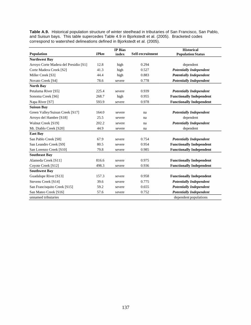
137

Table A.9. Historical population structure of winter steelhead in tributaries of San Francisco, San Pablo, and Suisun bays. This table supercedes Table 4.9 in Bjorkstedt et al. (2005). Bracketed codes correspond to watershed delineations defined in Bjorkstedt et al. (2005).

Population IPkm IP Bias index Self-recruitment


Northwest Bay Arroyo Corte Madera del Presidio [S1] 12.8 high 0.294 dependent Corte Madera Creek [S2] 41.3 high 0.527 Potentially Independent Miller Creek [S3] 44.4 high 0.883 Potentially Independent Novato Creek [S4] 78.6 severe 0.778 Potentially Independent North Bay Petaluma River [S5] 225.4 severe 0.939 Potentially Independent Sonoma Creek [S6] 268.7 high 0.955 Functionally Independent Napa River [S7] 593.9 severe 0.978 Functionally Independent Suisun Bay Green Valley/Suisun Creek [S17] 164.0 severe na Potentially Independent Arroyo del Hambre [S18] 25.5 severe na dependent Walnut Creek [S19] 202.2 severe na Potentially Independent Mt. Diablo Creek [S20] 44.9 severe na dependent East Bay San Pablo Creek [S8] 67.9 severe 0.754 Potentially Independent San Leandro Creek [S9] 80.5 severe 0.954 Functionally Independent San Lorenzo Creek [S10] 79.8 severe 0.985 Functionally Independent Southeast Bay Alameda Creek [S11] 816.6 severe 0.975 Functionally Independent Coyote Creek [S12] 498.3 severe 0.936 Functionally Independent Southwest Bay Guadalupe River [S13] 157.3 severe 0.958 Functionally Independent Stevens Creek [S14] 39.6 severe 0.775 Potentially Independent San Francisquito Creek [S15] 59.2 severe 0.655 Potentially Independent San Mateo Creek [S16] 57.6 severe 0.752 Potentially Independent unnamed tributaries dependent populations

Central California Coast Steelhead DPS

Russian Gulch (S)[d] Lower Russian tributaries Austin Creek Dutch Bill Creek Green Valley Creek Scotty Creek [d] Salmon Creek (S)[43] Bodega Harbor [44] Americano Creek [45] Stemple Creek [46] Walker Creek [TB1] Lagunitas Creek [TB2] Drakes Bay [48] Pine Gulch [49] Redwood Creek (Ma)[50]

Interior S. F. Bay

Arroyo Corte Madera del Presidio [S1]Corte Madera Creek [S2] Miller Creek [S3] Novato Creek [S4] Guadalupe River [S13] Stevens Creek [S14] San Francisquito Creek [S15] San Mateo Creek [S16]

Petaluma River [S5] Sonoma Creek [S6] Napa River [S7] Green Valley/Suisun Cr [S17]Arroyo del Hambre [18] Walnut Creek [S19] Mt. Diablo Creek [S20] San Pablo Creek [S8] San Leandro Creek [S9] San Lorenzo Creek [S10] Alameda Creek [S11] Coyote Creek [S12]

San Pedro Creek [e] Pilarcitos Creek [52] TunitasCreek [53] San Gregorio Creek [54]Pomponio Creek [55] Pescadero Creek [56] Arroyo de los Frijoles [e] Gazos Creek [57] Whitehouse Creek [e] Cascade Creek [e] Ano Nuevo Creek [e] Waddell Creek [58] Scott Creek [59] San Vicente Creek [60] Liddell Creek [e] Laguna Creek [61] Baldwin Creek [e] Wilder Creek [62] San Lorenzo River [63] Rodeo Creek Gulch [e] Soquel Creek [64] Aptos Creek [65]

North Coastal

Interior

Mark West Creek Middle Russian tributaries Dry Creek Maacama Creek Sausal Creek Upper Russian River [42]

Santa Cruz Mountains

Coastal S. F. Bay

Figure A.4. Historical structure of the CCC-steelhead DPS, arranged by diversity strata. Functionally independent populations are listed in bold font. Potentially independent populations are listed in bold-italic font. Dependent populations are listed in regular font. Not all dependent populations have been included in this figure. See table A.4 for complete list.

138

139

Coho Salmon Streams*PresentSuspected

PopulationFunctionally IndependentPotentially IndependentDependent Population

Diversity StrataLost Coast-Navarro PointNavarro Point-Gualala PointCoastalSan Francisco BaySanta Cruz Mountains

¯0 10 20 30 40 50

Miles

*Based on analyses of recent coho salmon presence developed byCalifornia Department of Fish & Game (February 2006 Draft). Not all coho streams are shown; nor do coho necessarily occur in depictedstreams in all years. Linework represents stream reaches that are knownor believed to be used by coho salmon. Observations are either present (direct observation) or suspected (indirect, anecdotal). 345 of these 405CCC Coho salmon observations occurred after 1990. Not all dependent populations are shown. See Table A.1 for complete list.

Map produced by David H. Hines and Charleen Gavette, NMFS, Santa Rosa, CA; modified by Ethan Mora and Brian Spence, NMFS,SWFSC, Fisheries Ecology Division.

Central California Coast Coho Salmon ESUDiversity Strata and Populations

San Mateo Cr.

ArroyoCorte

Madera

Russian Gulch

Little R.

Redwood Cr.

Caspar Cr.

Big Salmon Cr.

Pine Gulch Cr.

Hare Cr.

Russian Gulch

Gazos Cr.

Cottaneva Cr.

Wages Cr.

Corte Madera

Brush Cr.

Pudding Cr.

Waddell Cr.

Aptos

Pilarcitos Cr.San Francisquito Cr.

Miller Cr.

Stevens Cr.

Americano Cr.

San Gregorio Cr.

Salmon Cr.

Usal Cr.

Alder Cr.

Scott Cr.

Stemple Cr.

San Pablo Cr.

Elk R.

Soquel

San Leandro Cr.

San Lorenzo Cr.

Walker Cr.

San Lorenzo R.

Sonoma Cr.

Albion R.

Pescadero Cr.

Lagunitas Cr. Novato Cr.

Ten Mile R.

Garcia R.

Petaluma R.

Noyo R.

Guadalupe R.

Big R.

Gualala R.

Navarro R.

Coyote

Napa R.

Alameda Cr.

Russian R.

Plate A1. Diversity strata for populations of Central California Coast coho salmon. Based on Bjorkstedt et al. (2005) with modifications described in Appendix A.

140

Chinook Salmon Streams*

PopulationFunctionally Independent

Potentially Independent

Dependent Populations

Diversity StrataNorth Coastal



Central Coastal

California Coastal Chinook Salmon ESUFall Run

¯0 10 20 30 40 50

Miles

Redwood R.

Little R.

Mad R.

Humboldt Bay

Lower Eel R.

Bear R.

Mattole R.

Upper Eel R.

Usal Cr.

Cottoneva Cr.

DeHaven Cr.Wages Cr.

Ten Mile R.

Pudding Cr.Noyo R.Hare Cr.

Caspar Cr.

Big R.Albion R.

Big Salmon Cr.Navarro R.

Greenwood Cr.Elk Cr.

Brush Cr.Alder Cr.

Garcia R.

Gualala R.

Russian R.

*Based on NMFS (2005) designation of critical habitat(FRN 70 52488-52627). Not all Chinook-bearing streamsare necessarily shown.

Map produced by David H. Hines and Charleen Gavette, NMFS, Santa Rosa, CA; modified by Ethan Mora and Brian Spence, NMFS, SWFSC, Fisheries Ecology Division.

Diversity Strata and Populations

Plate A2. Diversity strata for populations of fall-run California Coastal Chinook salmon. Based on Bjorkstedt et al. (2005) with modifications described in Appendix A.

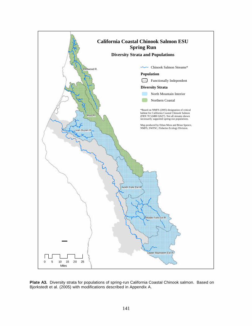
141

Van Duzen R.

Redwood R.

Mad R.

North Fork Eel R.

Middle Fork Eel R.

Upper Mainstem Eel R.

California Coastal Chinook Salmon ESUSpring Run


0 5 10 15 20 25Miles

¯

Chinook Salmon Streams*

Population

Functionally Independent

Diversity Strata


Northern Coastal

*Based on NMFS (2005) designation of critical habitat for California Coastal Chinook Salmon (FRN 70 52488-52627). Not all streams shown necessarily supported spring-run populations.

Map produced by Ethan Mora and Brian Spence, NMFS, SWFSC, Fisheries Ecology Division.

Plate A3. Diversity strata for populations of spring-run California Coastal Chinook salmon. Based on Bjorkstedt et al. (2005) with modifications described in Appendix A.

142

Redwood

Maple

Little (H)

Mad

Humboldt Bay

Van Duzen

Mc Nut

Lower MainstemEel

Price

HoweLarabee

Lower MiddleMainstem Eel

Dobbyn

North ForkEel

KekawakaJewett

Pipe

Chamise

BellSprings

Upper MiddleMainstem Eel

Woodman

Bear

Mattole

Guthrie

South ForkEel

Middle Fork Eel

Usal

Cottaneva

Wages

Ten Mile

Outlet

Bucknell

PuddingNoyo

Upper Mainstem EelSoda

BigCaspar

AlbionBig Salmon

NavarroGreenwoodElk

AlderBrush

Garcia

Gualala

Tomki

Northern California Steelhead DPSWinter Run


Steelhead Streams*


Potentially IndependentDependent

Diversity StrataNorthern CoastalNorth Mountain Interior

Lower Interior


Central Coastal

0 8 16 24 32 40Miles

¯

*Based on NMFS (2005) designation of critical habitat(70 FRN 52488-52627). Not all steelhead-bearing streams are shown.


Plate A4. Diversity strata for populations of winter-run Northern California steelhead. Based on Bjorkstedt et al. (2005) with modifications described in Appendix A.

143

Van Duzen R.

Redwood R.

Mad R.

Larabee Cr.

North Fork Eel R.

Middle Fork Eel R.

Mattole R.

South Fork Eel R.

Upper Mainstem Eel R.

Upper MiddleMainstem Eel R.

Dobbyn Cr.

Northern California Steelhead DPSSummer Run


Steelhead Streams*

PopulationFunctionally IndependentDependent Population

Diversity StrataNorth Mountain InteriorNorthern Coastal

0 5 10 15 20 25Miles

¯

*Based on NMFS (2005) designation of critical habitat for Northern California Steelhead (FRN 70 52488-52627). Distribution of summer-run fish was probably more limited than shown.


Plate A5. Diversity strata for populations of summer-run Northern California steelhead. Based on Bjorkstedt et al. (2005) with modifications described in Appendix A.

144

Lower Russian R.

Alameda Cr.

Napa R.

Coyote Cr.

Guadalupe R.

Novato Cr.

Sonoma Cr.

Petaluma R.

SanLorenzo R.

Lagunitas Cr.

Walker Cr.

Pescadero Cr.

Stemple Cr.

Salmon Cr.

San Gregorio Cr.

Americano Cr.

Stevens

Miller Cr.

SanFrancisquito Cr.

Pilarcitos Cr.

Scott Cr.

Waddell Cr.

CorteMadera Cr.

Gazos Cr.

Tunitas Cr.

Pine Gulch

Redwood Cr.

ArroyoCorte

Madera

Pomponio Cr.

Laguna Cr.

Wilder Cr. Soquel Cr.Aptos Cr.

SanMateo Cr.

San Lorenzo Cr.

SanLeandro Cr.

San Pablo Cr.

Maacama Cr.

Mark West Cr.

GreenValley Cr.

Austin Cr.

Dry Cr.

Upper Russian R.

San Vicente Cr.

Drakes Bay

Sausal Cr.

DutchBill Cr.

MiddleRussian R.

Bodega Harbor

Green Valley/Suisun Cr.

Walnut Cr.

Mt Diablo

Arroyo delHambre

Central California Coast Steelhead DPS

¯0 5 10 15 20 25

Miles

*Based on NMFS (2005) designation of critical habitat (70 FRN 52488-52627). Not all steelhead-bearingstreams are shown.

Map produced by David H. Hines and Charleen Gavette, NMFS, Santa Rosa, CA; modified by Ethan Mora and Brian Spence, NMFS, SWFSC, Fisheries Ecology Division.


Steelhead Streams*


Potentially IndependentDependent Population

Diversity StrataInteriorNorth Coastal

Interior S.F. BayCoastal S.F. Bay

Santa Cruz Mountains

Plate A6. Diversity strata for populations of Central California Coast steelhead. Based on Bjorkstedt et al. (2005) with modifications described in Appendix A.

145

Appendix B. Discussion of Density Criteria and their Application As noted in the main body of this report, the NCCC TRT spent substantial time discussing the

appropriateness and application of density criteria. Much of the discussion revolved around four central

issues: (1) how to estimate density in situations where substantial habitat is no longer accessible due to

impassible or so degraded as to preclude use by salmonids; (2) whether the density criteria (or abundance

targets dictated by density criteria) for populations at “low risk” were sufficiently precautionary or overly

so; (3) whether it was more appropriate to express density criteria in terms of fish per IPkm or fish per

total accessible kilometers; and (4) whether adjustments to the criteria should be made to account for

potential bias in estimates of IP. The first of these issues was covered in the main body of this report.

The remaining three issues are treated in the sections that follow.

Are the density criteria sufficiently precautionary or overly so?

During the course of our discussions, some TRT members initially expressed concern that the

implementation of low-risk density criteria might result in abundance targets that are unrealistically high

for certain watersheds (i.e., they might exceed what was historically possible), particularly in watersheds

where the IP bias index (see discussion below) suggests that the IP model may overestimate historical

habitat potential. Conversely, other TRT members worried that perhaps the criteria might not be

precautionary enough. Ultimately, the TRT concluded that the proposed density criteria—40 spawners

per IP-kilometer for watersheds with the minimum amount of potential habitat (IPkm) thought to be

capable of sustaining an independent population, declining to 20 spawners per kilometers for watershed

with 10-fold the habitat potential of the minimum watershed—represented a reasonable “floor” for

interim criteria in lieu of more sophisticated population viability analyses.

This conclusion is based on several lines of reasoning. First, recall that for each species, we have defined

a minimum threshold of potential habitat (32 IPkm for coho salmon, 20 IPkm for Chinook salmon, and 16

IPkm for steelhead) that was required for the population to be considered viable in isolation when

populations were functioning at or near their historical carrying capacity. Thus, estimates of carrying

capacity in relatively undisturbed systems might provide a reasonable basis for determining spawner

density criteria for these smallest systems. Unfortunately, the scientific literature lacks estimates of

carrying capacities for relatively pristine systems. Our estimate of 40 spawners/IPkm was based on the

analysis of Bradford et al. (2000), who examined inflection points in hockey-stick stock-recruitment

curves for 14 coho salmon populations and found that on average full smolt recruitment occurred at

spawner densities of 19 female per kilometer (which assuming a sex ratio slightly biased in favor of males

146

translates to roughly 40 spawners/km). In using this value as the basis for spawner density criteria,

several things should be kept in mind. First, the watersheds used to estimate spawner densities at full

smolt recruitment represented habitats with varying levels of human disturbance, with few in relatively

pristine condition. Thus, historical carrying capacities were, in all probability, somewhat higher on

average than those suggested by data collected post human disturbance. Additionally, to estimate

spawner densities, Bradford et al. (2000) divided adult spawner abundance by an estimate of total

accessible kilometers of habitat (although they acknowledge that, in some cases, these estimates may not

include all possible habitat). In contrast, the NCCC TRT proposes using IPkm as the denominator in

calculating density (see discussion below). Within the NCCC Recovery Domain, the ratio of IPkm to

total accessible kilometers typically averages about 0.6 for coho salmon. Assuming that this ratio is

similar in other streams in the Pacific Northwest, this would again suggest that densities at carrying

capacity may have been higher than suggested by our density criteria.

Ideally, information on historical population abundance prior to extensive human disturbance could

provide a means of validating the proposed density criteria. Unfortunately, data on historical adult

abundance of salmon and steelhead are extremely scarce in the NCCC Recovery Domain, and where such

estimates are available, they are for time periods during and after substantial human-caused impacts had

already occurred. The only published comprehensive (in geographic scope) coastwide estimates of

historical abundance are contained in a report prepared by CDFG (1965). Additionally, there are

historical counts of salmon and steelhead at two dams in the domain (Benbow Dam on the South Fork Eel

River and Sweasy Dam on Mad River), as well as of coho salmon and steelhead at Waddell Creek. In the

sections below, we compare these historical estimates with our abundance targets. Further, we apply our

density criteria to populations in nine coastal watersheds of Oregon and compare projected abundance

targets with estimates derived from cannery pack records from the late 1800s and early 1900s.

Comparison of population abundance targets with historical estimates of abundance

1965 CDFG coastwide estimates

A report published by CDFG (1965) provides estimates of abundance of Chinook salmon, coho salmon

and steelhead for most major watersheds in California. For coasta l watersheds, these estimates are based

primarily on the professional judgment of local biologists working in the area, who “made comparisons

with better-studied streams” and, in a few instances, had some additional data to assist them, such as dam

counts (e.g. Mad and Eel rivers) or harvest information. Though there is very high uncertainty

surrounding these estimates, they nevertheless provide the only basis for assessing whether the abundance

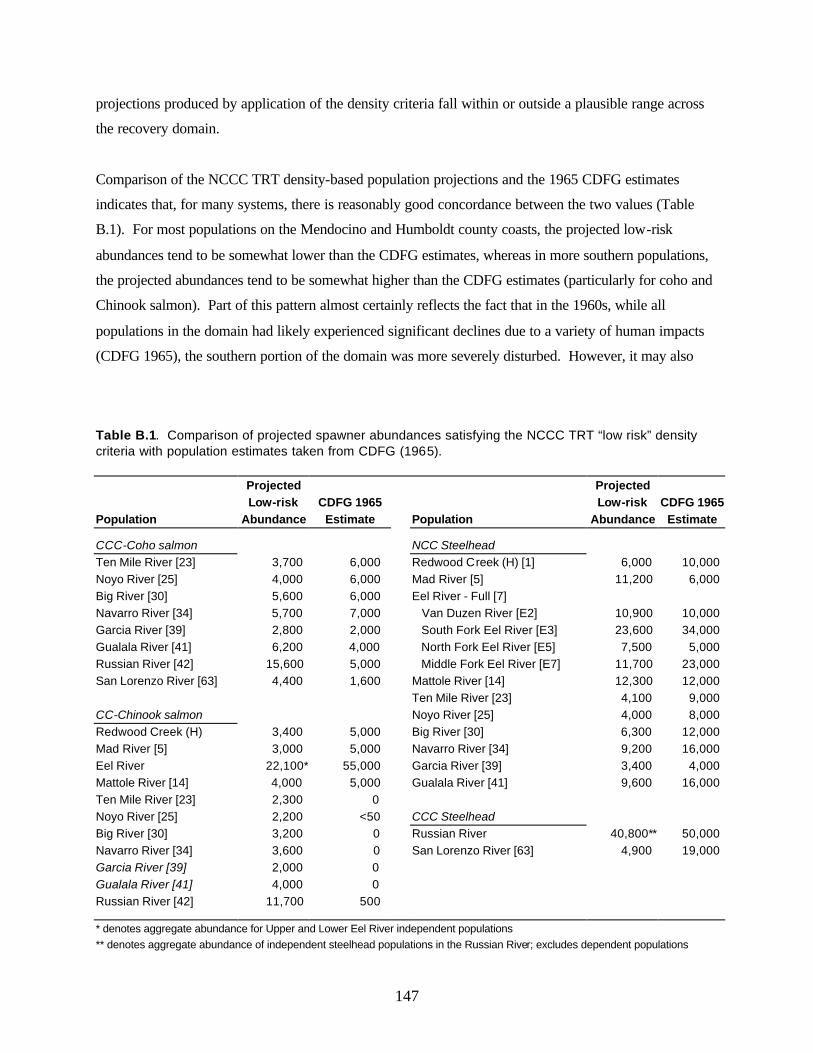
147

projections produced by application of the density criteria fall within or outside a plausible range across

the recovery domain.

Comparison of the NCCC TRT density-based population projections and the 1965 CDFG estimates

indicates that, for many systems, there is reasonably good concordance between the two values (Table

B.1). For most populations on the Mendocino and Humboldt county coasts, the projected low-risk

abundances tend to be somewhat lower than the CDFG estimates, whereas in more southern populations,

the projected abundances tend to be somewhat higher than the CDFG estimates (particularly for coho and

Chinook salmon). Part of this pattern almost certainly reflects the fact that in the 1960s, while all

populations in the domain had likely experienced significant declines due to a variety of human impacts

(CDFG 1965), the southern portion of the domain was more severely disturbed. However, it may also

Table B.1. Comparison of projected spawner abundances satisfying the NCCC TRT “low risk” density criteria with population estimates taken from CDFG (1965). Projected Projected Low-risk CDFG 1965 Low-risk CDFG 1965 Population Abundance Estimate Population Abundance Estimate CCC-Coho salmon NCC Steelhead Ten Mile River [23] 3,700 6,000 Redwood Creek (H) [1] 6,000 10,000 Noyo River [25] 4,000 6,000 Mad River [5] 11,200 6,000 Big River [30] 5,600 6,000 Eel River - Full [7] Navarro River [34] 5,700 7,000 Van Duzen River [E2] 10,900 10,000 Garcia River [39] 2,800 2,000 South Fork Eel River [E3] 23,600 34,000 Gualala River [41] 6,200 4,000 North Fork Eel River [E5] 7,500 5,000 Russian River [42] 15,600 5,000 Middle Fork Eel River [E7] 11,700 23,000 San Lorenzo River [63] 4,400 1,600 Mattole River [14] 12,300 12,000 Ten Mile River [23] 4,100 9,000 CC-Chinook salmon Noyo River [25] 4,000 8,000 Redwood Creek (H) 3,400 5,000 Big River [30] 6,300 12,000 Mad River [5] 3,000 5,000 Navarro River [34] 9,200 16,000 Eel River 22,100* 55,000 Garcia River [39] 3,400 4,000 Mattole River [14] 4,000 5,000 Gualala River [41] 9,600 16,000 Ten Mile River [23] 2,300 0 Noyo River [25] 2,200 <50 CCC Steelhead Big River [30] 3,200 0 Russian River 40,800** 50,000 Navarro River [34] 3,600 0 San Lorenzo River [63] 4,900 19,000 Garcia River [39] 2,000 0 Gualala River [41] 4,000 0 Russian River [42] 11,700 500 * denotes aggregate abundance for Upper and Lower Eel River independent populations ** denotes aggregate abundance of independent steelhead populations in the Russian River; excludes dependent populations

148

reflect a north-south gradient in the degree of IP -bias (discussed below). Overall, however, comparison

with the 1965 estimates strengthens the argument that the projected abundances are within a plausible

range. We do note, however, that if the 1965 abundance estimates, made at a time when habitat

degradation from land and water use were already widespread, are even somewhat close to true

abundances, then the density-based low-risk abundances suggested by our criteria are more appropriately

viewed as minimum “floors,” rather than indicative of historical carrying capacities.

Waddell Creek coho salmon and steelhead estimates

Adult population abundance estimates are available for both coho salmon and steelhead in Waddell Creek

from the study of Shapovalov and Taft (1954). Adult salmon and steelhead were counted at a weir placed

about 2.5 km upstream of the ocean and 1 km above the uppermost extent of tidewater. During the nine-

year period covering spawning seasons 1933-34 to 1941-42, the average annual adult (including jacks)

run size for coho salmon was estimated to be 313 (range 111-748). During the same period, the estimated

abundance of adult steelhead was 481 (range 428-554) 33.

Bjorkstedt et al. (2005) concluded that Waddell Creek likely supported a dependent population of coho

salmon, as total IPkm in the basin (9.12 IPkm) was only about 29% of that deemed necessary to support

an independent population. Nevertheless, if we were to apply the density of spawners used to produce

abundance targets for the smallest independent populations (i.e., 40 spawners per IPkm), we would arrive

at an estimated abundance of about 365 spawners for coho salmon. For steelhead, we estimated a total of

16.24 IPkm for the Waddell Creek basin, which translated to a target abundance of 649 spawners (which

we rounded to 600) for this independent population. Consequently, the estimated historical abundance

between 1933 and 1942 averaged about 86% and 80% of the projected abundance targets for coho salmon

and steelhead, respectively, based on a spawner density of 40 spawners per IPkm.

Although the density-based abundance targets are slightly higher than abundances recorded in the 1930s

and 1940s, it is important to consider the historical context. Foremost, the condition of the Waddell

Creek watershed at the time of the Shapovalov and Taft study was far from pristine. Shapovalov and Taft

(1954) describe Waddell Creek in the following terms:

“ Some changes from the primitive condition of the area have taken place as a result of human

usage. The redwood forest of the watershed below Big Basin was logged off by 1870 and is now 33 Estimated run sizes include weir counts plus estimates of numbers of adults that spawned below the weir or that jumped over the weir during high flows. Coho salmon and steelhead totals from Table 9 (pg. 47) and Table 35 (pg. 138), respectively, in Shapovalov and Taft (1954).

149

covered by a second growth. The early lumbering operations have resulted in the creation of

several semipermanent log jams and temporary accumulations of logs, which have hastened

erosion of the stream banks, with consequent increase in silting during flood stage.”

The statements of Shapovalov and Taft likely understate the degree to which Waddell Creek had been

affected by clearing of the redwood forests. The first steam sawmill in Santa Cruz County was built near

the confluence of the East and West forks of Waddell Creek in 1862, and the basin was heavily logged

between 1862 and 1875. Big Basin Redwoods State Park was established in 1902 to protect the last

significant stand of old-growth redwoods in the Santa Cruz Mountains 34. At the time Shapovalov and Taft

conducted their research, Big Basin State Park covered an area of fewer than 10,000 acres, all of which

was in the headwater regions of Waddell Creek basin, upstream of the two known natural barriers to

anadromy on the East and West branches of Waddell Creek. (Major additions to the park, including the

middle and lower reaches containing most of the coho salmon and steelhead habitat, came between the

late 1950s and 1980s). Consequently, virtually all portions of the watershed accessible to coho salmon

had been extensively disturbed prior to the onset of Shapovalov and Taft’s study. We do not believe it

unreasonable to think that such disturbance would have resulted in at least a 20%-25% reduction in

productive capacity for coho salmon and steelhead. Consequently, we do not believe that density-based

criteria produce predictions of capacity that are unrealistic for either species. This is encouraging because

Waddell Creek lies near the southern edge of the coho salmon’s historical range, where bias associated

with the IP model is expected to be greatest.

We note that there were two active hatcheries in Santa Cruz County during the period Shapovalov and

Taft conducted their study. However, our review of historical records indicate that coho salmon and

steelhead were planted into Waddell Creek on only a few occasions and in small numbers during the

Shapovalov and Taft years35. Specifically, Waddell Creek received a planting of 15,000 coho salmon fry

in 1933 and plantings of steelhead fry totaling 36,000 fish in 1930, 34,000 fish 1932, and 1,005 fish 1933.

We conclude that the potential influence of stocking on the adult counts was likely small for the following

five reasons: (1) the total numbers of fish stocked were small; (2) the stocked fish were primarily fry

(except perhaps the 1,005 steelhead released in 1933), which typically have very low survival rates; (3)

the duration of stocking was limited to one of eight years for coho salmon and three of eight years for

steelhead (with only 1,005 fish released in one of those years); (4) the majority of steelhead were released

34 A second smaller old-growth redwood stand (about 40 acres) remained unharvested near Felton. 35 Source: State of California, Department of Natural Resources, Division of Fish and Game, Record of Fish Distributions. Compiled by Dayes (1987).

150

in the headwaters of Big Basin State Park, upstream of barriers to anadromy; and (5) adult counts in years

following stocking are not obviously higher or lower than in years without planting. Therefore, we

consider the counts to be a reasonable indicator of the natural carrying capacity for this period.

Eel River coho salmon, Chinook salmon, and steelhead.

Counts of coho salmon, Chinook salmon, and steelhead were made at Benbow Dam on the South Fork

Eek River from 1938 to 1975. Benbow Dam was located about 133 km upstream of the ocean, and about

67 km upstream of where South Fork Eel River enters the mainstem. Counts at this dam, consequently,

represent only a portion of the independent populations of Chinook salmon, coho salmon, and steelhead

delineated in the population structure report.

To compare historical abundance estimates with density-based projections for coho salmon, Chinook

salmon, and steelhead, we estimated the fraction of total IPkm for each population that occurred upstream

of the Benbow Dam and then multiplied this fraction by the overall abundance targets to obtain estimates

of the contribution of above-dam habitats to the total population targets. We then compared these

estimates to historical counts from 1938 to 1950 at the dam. This time period was presumed to be when

the influence of human impacts was lowest (for the period of record), as evidenced by the fact that counts

during these periods were generally higher on average than in the decades that followed. We note that the

period 1938 to 1950 does not represent a particularly favorable period with respect to oceanic conditions.

Data presented in Hare et al. (1999) indicates that commercial catch of coho salmon in California and

Oregon was relatively low from 1938 through the mid-1950s, and then increased substantially from the

late 1950s into the mid-1970s. This contrasts with the Benbow Dam coho counts, which averaged only

about 30% of the 1938-1950 counts from 1951 to 1975. The continued decline of coho in the South Fork

Eel after 1950, when production was increasing elsewhere in the California Current system, indicates that

the high counts recorded in the 1930s and 1940s were not the result of unusually favorable ocean

conditions. In fact, the first half of this period occurred during a positive phase of the Pacific Decadal

Oscillation, conditions that typically result in lower salmon production in Oregon, Washington, and

California (Hare et al. 1999).

For the South Fork Eel River, our density-based abundance projections for populations upstream of

Benbow Dam were 6,836 for coho salmon, 4,415 for Chinook salmon, and 15,732 for steelhead36. In all

three cases, these projections are well below the recorded average abundances for these three species 36 Because the total IPkm for coho salmon, Chinook salmon, and steelhead populations that include the South Fork Eel River basin are 10 times the minimum IPkm required for an independent population, we assume a spawner density of 20 spawners per IPkm for all three species. Data on historical counts from StreamNet (Available online at: www.streamnet.org).

151

during the 1938-1950 period (Table B.2): projected abundances were about 51%, 37%, and 91% of the

dam counts for coho salmon, Chinook salmon, and steelhead during the period. Thus, there is strong

evidence that our methods do not overestimate the historical carrying capacities of these three species in

the South Fork Eel River basin upstream of Benbow Dam (see further discussion below).

Our conclusion gains strength when we consider that, for a number of reasons, the counts at Benbow Dam

underestimate the total population sizes for the South Fork Eel River. First, the fish counts at Benbow

Dam do not take into account harvest of salmon in ocean and in-river fisheries downstream of the dams,

which was considerable during the late 1930s to 1950s. Although commercial catch statistics for

California are generally not available for this period (INPFC 1979), local newspaper accounts indicate

that recreational fishers were deeply concerned that ocean troll fisheries were severely depleting Eel River

salmon populations during this time. One article in the Ferndale Enterprise from September 1937 reports

that commercial troll fishers harvested about 100,000 lbs of salmon in a single day in the waters off of the

Eel River mouth. They protested that this equated to about 5,000 20-lb Chinook salmon, which was more

than the total take in sport fisheries for an entire season (Van Kirk 1996d).

Second, the counts at Benbow Dam were likely influenced by the legacy of historical commercial net

(seine and gill-net) fisheries that operated in the lower Eel River from the 1850s into the 1920s. By the

1890s, these fisheries had caused a precipitous decline in the number of salmon returning to the Eel River.

Between 1877 and 1889, canneries in the lower Eel River basin processed in the neighborhood of three-

quarters of a million pounds of salmon annually. Increasing public concern resulted in prohibitions on

seining in 1913 and gill-netting in 1922 (Lufkin 1996). Commercial troll fishing was initiated in 1916

and soon replaced the net fisheries as the dominant Eel River fishery. Newspaper accounts in the 1930s

and 1940s periodically make reference to the devastating impact that net fisheries had on Eel River

salmon populations, from which the populations apparently never fully rebounded (Van Kirk 1996a,b,c).

Table B.2. Comparison of average historical (1938-1952) counts of adult migrant coho salmon, Chinook salmon, and steelhead at Benbow Dam, South Fork Eel River, with density-based abundance targets developed by the TRT.

Population

Historical counts of adult migrants: Mean (range)

Years

Total IPkm above dam

Projected number of spawners above dam

based on density criteria S. Fk. Eel River Coho salmon

13,514 (7,370-25,289)

1938-1950

341.8

6,836

S. Fk. Eel River Chinook salmon

11,782 (3,424-21,011)

1938-1950

220.8

4,415

S. Fk. Eel River steelhead

17,343 (12,995-25,032)

1938-1950

786.6

15,732

152

Third, a significant amount of habitat degradation had likely already occurred in the South Fork Eel River

by the late 1930s, when the counts began. Logging of the coastal redwood forests, which began in the

1800s throughout much of the North Coast, began somewhat later in the South Fork Eel River basin, due

to the fact that much of the drainage was not easily accessible by road (BLM et al. 1996). However,

completion of the Redwood Highway (Hwy 101) in the late 1920s, which runs along the South Fork Eel

River, allowed rapid expansion of logging in the South Fork Eel River basin.

Fourth, for a number of reasons, counts at Benbow Dam almost certainly underestimate the total number

of fish that passed upstream of the dam. The weekly reports prepared by those operating the Benbow

Dam facilities indicate that there were two ladders (south and north) around the dam. During the 1937-38

and 1938-39 seasons, both ladders were monitored on a regular basis. However, frequent landslides

plagued the north ladder, and by the 1940-41 season, counts were made almost exclusively at the south

ladder. The degree to which rocks and soil deposited into the north ladder precluded use by salmon and

steelhead is uncertain. However, various notes from the weekly reports indicate that, under certain flow

conditions, the number of fish using the north ladder was substantial and even exceeded numbers using

the south ladder37. Indeed, a memo written by Shapovalov (1946) indicates that the ladder operator

during the 1944-45 and 1945-46 seasons estimated that 900 steelhead passed through the north fishway

during the 1945-1946 season (about 7% of the number of steelhead counted at the south ladder that year),

and that 1,000 salmon and steelhead passed through the north ladder in the 1945-1946 season (about 2%

of the south ladder count). These estimates are not included in the published annual totals. The same

operator made a note on March 19, 1945 that he saw “a few fish hurdling No. [north] ladder. Same

condition has been going on for 3 years, so absurd to change tallies now.” (Coons 1945). Thus, it

appears safe to assume that passage of uncounted fish through the north ladder was a fairly regular

occurrence. Additionally, notes on water clarity were routinely made in the weekly reports, and they

frequently describe the water a muddy, murky, or cloudy. In some cases, the observers make reference to

“difficult conditions” for census work. Under such conditions, it seems likely that some fish were missed

by observers. And finally, there were many instances where flows were so high that the station had to be

closed. Collectively, these pieces of evidence indicate that the counts should be viewed as partial counts,

Although there is no means for estimating what fraction of the total run was sampled in any given year,

suffice it to say that total escapement likely exceeded the recorded counts.

37 All indications are that the north ladder effectively passed fish under a narrower range of flow conditions than did the south ladder.

153

Finally, it is well documented that in the first years of operation (1932-1937), the fish ladders at Benbow

Dam functioned poorly, which prompted considerable public concern and outrage (Van Kirk 1996d). On

February 28, 1936, the Ferndale Enterprise wrote:

“The soul-sickening spectacle of thousands of splendid steelhead and salmon—all heavy with

spawn—sentenced to a miserable death without completing their life cycle because the Department of

Natural Resources State of California has failed to provide adequate fish ladders at Benbow Dam, on

the Eel River, has aroused sportsmen of that district”

It is unclear how problems with fish passage in the mid-1930s may have affected populations in

subsequent years, but it seems safe to assume that any effect was negative.

All of these pieces of evidence would suggest 1) that carrying capacities during the period 1938-1950

were substantially higher than counts at Benbow Dam would indicate, and 2) that historical capacities

prior to arrival of Euro-Americans were likely higher still by a good margin.

Conversely, there was some hatchery activity during the 1930s and 1940s on the Eel River, which

potentially could artificially inflate adult counts at Benbow Dam. A few hatcheries operated in Humboldt

County during this period. The most likely candidate for plants into the Eel River was the Fort Seward

Hatchery. Fort Seward hatchery, which operated from 1916 to 1941 was located on the Eel River

mainstem approximately 36 km upstream of the confluence of the South Fork. Between 1935 and 1941,

the hatchery distributed an average of about 579,000 steelhead and 480,000 Chinook salmon to streams

and rivers of Humboldt County, with an additional 170,000 steelhead on average going to streams in

Mendocino County from 1938 to 1941. Coho salmon were also released from 1935-1938, with an

average annual total of about 693,000. Unfortunately, the distribution locations of these fish are not

known; thus, it is unclear if any of these fish (and if so, how many) were released into the South Fork Eel

River and so may have influenced counts at Benbow Dam.

We do note that Benbow Dam counts before and after the “plausible” stocking periods indicate no clear

changes in abundance. Counts of Chinook salmon were slightly lower (~11,000) during the period

potentially affected by stocking (1938-1944) than in 1945-1950, the period following stocking, when the

average count was about 12,700 adults. Likewise, counts of coho salmon from 1938-1940 (the years that

would have been directly affected by plantings if they occurred in the South Fork) are lower on average

(~9,400) than those in the period from 1941-1950 (~14,900) when no planting occurred. Only for

154

steelhead were counts at Benbow dam slightly lower (~15,600) in the years after stocking (1945-1950)

than in the years potentially affected by stocking (1938-1944; average ~18,800). Again, we have no

direct evidence that stocking actually took place in the South Fork Eel. But the lack of evidence of

substantial population declines when Fort Seward hatchery ended production indicates that any effects of

stocking were either small or swamped out by other factors.

Mad River coho salmon, Chinook salmon, and steelhead.

Counts of coho salmon, Chinook salmon, and steelhead were made at Sweasy Dam on the Mad River

from 1938 to 1964. Sweasy Dam was located some 15 km upstream of the river mouth. Thus, counts at

the dam represent only a portion of the total population sizes for the Mad River basin. Density-based

projections for coho salmon, Chinook salmon, and steelhead were made by estimating the percentage of

total IPkm for each population that occurred upstream of Sweasy Dam (27%, 51%, and 76% for coho

salmon, Chinook salmon, and steelhead, respectively) and then multiplying this fraction by the overall

abundance targets to obtain estimates of the contribution of above-dam habitats to the total population

targets. These estimates were then compared to historical counts from 1938 to 1950 at the dam, as again,

this period likely was the least affected by human activities.

For the Mad River, comparison of projected abundances versus historical counts produces more equivocal

results. Abundance projections for populations upstream of the Sweasy Dam were 1,334 for coho

salmon, 953 for Chinook salmon, and 8,430 for steelhead (Table B.3)38. For Chinook salmon, the average

count from 1938 to 1950 exceeds projected abundance by about 38%. Conversely, for coho salmon and

Table B.3. Comparison of average historical counts of adult migrant coho salmon, Chinook salmon, and steelhead at Sweasy Dam, Mad River from 1938-1950 compared with density-based abundance targets developed by the NCCC TRT.

Population

Historical counts of adult migrants:

Mean (range)

Years

Total IP above dam (% of basin total)

Projected number of spawners above dam

based on density criteria Mad River coho salmon

395 (73-515)

1938-1950

41.7

1,334

Mad River Chinook salmon

1,312 (484-3,139)

1938-1950

47.7

953

Mad River steelhead

4,401 (3,110-6,650)

1938-1950

421.5

8,430

38 For Chinook salmon and steelhead, total IPkm for the Mad River basin exceed 10 times the minimum IPkm required for an independent population; thus, we assume a spawner density of 20 spawners per IPkm for these two species. For coho salmon, the minimum required spawner density for a basin with 152.9 IPkm is 32 spawners/IPkm.

155

steelhead, the projected abundances exceed the average historical dam counts. Thus, while the historical

data indicate that the abundance projections do not over-predict historical carrying capacity for Chinook

salmon, the same cannot be said for coho salmon and steelhead at first glance. We do note that the

projected abundance for steelhead is subject to substantial uncertainty, as a considerable amount of

predicted IPkm lies upstream of a partial natural barrier near Bug Creek that apparently can limit access to

a substantial amount of habitat in some years.

There remains uncertainty as to operating procedures at the fish ladder and whether there existed the

capability to block fish passage during periods when counts were not made. We attempted to obtain

information from California Department of Fish and Game regarding dam and counting operations, but

thus far no one has come forth with definitive information that would enable us to ascertain whether the

counts represent full or partial counts, though obtaining full counts at any such facilities under all flow

conditions is usually quite difficult.

A second potential reason that dam counts for coho salmon and steelhead were lower than predicted by

our model likely relates to the condition of the Mad River watershed at the time counts were made.

Extensive clearing of the redwood forests along the Mad River downstream of Bug Creek (the apparent

upper distributional limit coho and Chinook salmon) had occurred by the end of the 1800s (Carranco

1982; HBMWD 2004). Undoubtedly, substantial modification of habitat, including removal of large

wood, loss of riparian canopy, increased sedimentation, and other impacts of logging had substantially

reduced carrying capacity of the Mad River and its tributaries at the time the dam counts were made.

Additionally, the Mad River was subject to splash and crib dams, along with log drives during the early

logging period (Carranco 1982). These activities would have resulted in substantial modification of

habitat. Because roads and other transportation mechanisms were lacking, logs were typically moved

downstream using several different types of dams. Splash dams were constructed across the stream

channel to impound the river. Logs were dragged into the impoundment behind the dam or the stream

channel below the dam. Water was then released suddenly by opening flood gates or blasting with

explosives, and the water, logs, and anything their path was carried down the river until they were hung

up on the next obstruction, where the splash-damming process was repeated. In other cases, semi-

permanent crib or frame dams were built to impound water so that logs could be floated down from

upstream or, when released, could transport logs downstream. Sometimes, release of water from multiple

dams was carefully timed to facilitated transport of logs downstream. Often times, crews cut out any

accumulations of wood downstream of a splash or crib dam to facilitate passage of logs when the dams

156

were blasted or water was released. Cutaway dams were dams that were used only once, often to “float”

logs that had accumulated in massive log jams resulting from splash and crib dam operations.

Collectively, dam and log drive activities would have severely scoured stream channels, resulting in

highly simplified habitats, reductions in the gravel remaining for spawning, and decreased stability of

gravels during high flow conditions. Such impacts would have been particularly harmful to Chinook and

coho salmon upstream of Sweasy Dam (particularly above Blue Slide Creek), as most of the potential

habitat in this reach lies in the mainstem, rather than the steep tributaries that characterize this reach.

Density-based targets compared with historical abundance estimates for Oregon coho salmon

In addition to comparing TRT abundance targets with historical records from within the NCCC recovery

domain, we also compared projected target abundances that would result if we applied our IP-based

density criteria to populations with estimates of historical adult abundance for nine coasta l watersheds in

Oregon. The Oregon abundance estimates were based on cannery records from 1892 to 1915 (from

Meengs and Lackey 2005). Meengs and Lackey (2005) estimated historical run sizes from cannery pack

records through a series of steps including 1) converting salmon pack data (in cases) into pounds of

salmon caught (by assuming a certain constant “waste” in processing); 2) converting pounds of salmon

captured into numbers of adult fish (by assuming an average weight for adult fish of 4.46 kg); 3)

converting numbers of harvested salmon into an estimate of total population sizes (assuming a specific

catch efficiency rate); and 4) using abundance estimates from the five years of highest cannery pack in

each watershed as indicative of run size39. Several other authors have estimated run sizes from cannery

pack records using slightly different methods and assumptions (see e.g., Mullen 1981, Lichatowich 1989,

Lawson et al. 2007), but overall the estimates derived by the various methods are generally fairly similar.

We therefore present only the results of Meengs and Lackey (2005).

Estimation of projected target abundances using the NCCC TRT density criteria was straightforward. We

obtained estimates of total coho salmon IPkm for each of the nine watersheds for which cannery records

were available. Intrinsic potential coverages were provided by the CLAMS project (Kelly Burnett and

Kelly Christiansen, US Forest Service, Pacific Northwest Research Station, Corvallis, Oregon). In

calculating IPkm, we considered only reaches downstream of natural barriers (including barriers that have

since been removed) so that the IPkm reflects those reaches historically available to coho salmon at the

turn of the 20th century. For all nine populations, the estimated IPkm exceeded 320, or ten times the

amount of IPkm required for population independence. Consequently, the target spawner density was

39 Cannery pack is a function not only of numbers of fish, but also market forces. Consequently, years of highest cannery pack are not necessarily the years of highest abundance.

157

assumed to be 20 spawners per IPkm, and the target abundance 20 times the total IPkm for the watershed

(see Table B.4).

A plot of IPkm versus historical estimates of abundance derived from cannery records (Figure 1) shows

that there is a reasonably strong correlation between IPkm and historical abundance in these watersheds

(R2 = 0.51). When abundance is regressed against estimates of stream miles accessible to coho salmon

unadjusted for IP, the relationship is slightly weaker (R2 = 0.48)40. These results contributed to the NCCC

TRT’s confidence that the IP model provides a reasonable basis for scaling habitat.

Much more importantly, the data in Table B.4 indicate that for Oregon Coast coho salmon populations the

abundance targets that would result from application of our density-based criteria are well below—by an

order of magnitude—historical estimates of abundance. In all cases, the target abundance expressed as a

percent of the historical estimates of abundance fall between about 3% and 12%. Thus, during the late

1800s and early 1900s, a period during which logging (and splash damming) was already well underway

(Seddell and Luchessa 1982), spawner densities of coho salmon in coastal watersheds of Oregon were

generally 10-fold to 20-fold higher than those required by our viability criteria. Even if we assume

substantial bias in the IP model for the southern portion of the range, which lies in the NCCC Recovery

Domain, it seems very unlikely that historical densities were lower than those the TRT has proposed for

viability.

Table B.4. Comparison of historical abundance estimates and hypothetical density-based abundance targets for coastal watersheds in Oregon.

Population

Historical estimates of abundance derived from

cannery records (Meengs & Lackey 2005)

IPkm

Estimated historical

spawner density (Spawners/IPkm)

Projected abundance target

based on MRD (20 spawners/IPkm)

Projected abundance target

as percent of historical estimate

Nehalam 236,000 1,116 211 22,300 9.3% Tillamook 234,000 537 436 10,700 4.7% Nestucca 107,000 299 358 6,000 5.6% Siletz 122,000 310 394 6,200 4.9% Siuslaw 547,000 902 607 18,000 3.3% Yaquina 65,000 385 169 7,700 12.3% Alsea 153,000 466 328 9,300 5.9% Coquille 342,000 883 387 17,700 5.3% Coos 161,000 552 292 11,000 6.8%

40 One might have expected IP to predict more of the variability; however, average IP scores are fairly constant across the nine coastal watersheds (range 0.56 to .67). Thus, the ability to evaluate whether IPkm is a better predictor of abundance than unadjusted stream kilometers is limited.

158

Figure B.1. Relationship between historical abundance, as estimated from cannery records (Meengs and Lackey 2005), and IPkm for nine coastal watersheds in Oregon.

Should density criteria be expressed in terms of IPkm or total accessible km?

Another issue that faced the TRT was whether density criteria should be expressed in terms of spawners

per IPkm or total accessible kilometers within a watershed. In the literature, spawner densities (including

those in Bradford et al. 2000) are obviously most commonly expressed in terms of spawners per kilometer

of stream. However, productive capacity within and among watersheds may be highly variable depending

on the nature and quality of habitats. For example, for coho salmon, certain habitat types such as alcoves

and dam pools typically found in unconstrained, low-gradient reaches of small-to-moderate-sized streams

often account for a disproportionate portion of the total smolt production in a system (Nickelson et al.

1992). Thus, streams with comparable numbers of total accessible miles may produce substantially

different numbers of fish. The IP models seek to predict such differences in the potential for different

stream reaches (and watersheds) to express habitat characteristics that are likely to be favorable to each

species, and thus we chose to use the aggregate IPkm in each watershed as the basis for density

calculations. Doing so assumes that, in general, density increases in direct proportion to the IP value for a

reach, which may not be entirely true (and is difficult to validate in the absence of reference streams that

have not been altered by human activities). However, the fact that estimates of IPkm were correlated with

historical estimates of total abundance in coastal watersheds or Oregon (Figure 1) and provided some

improvement in explanatory power over an unadjusted estimate of accessible stream kilometers suggests

that IPkm provides a reasonable basis for scaling differences in density criteria (and resulting abundance

projections) among watersheds.

y = 363.84x - 1722.5 R2= 0.5113

-

100,000

200,000

300,000

400,000

500,000

600,000

200 300 400 500 600 700 800 900 1000 1100 1200

IPkm

159

Should adjustments to density criteria be made to account for potential IP Bias?

In our population structure report, the TRT acknowledged potential bias in the IP model that may arise

due to regional differences in precipitation-runoff relationships or other local factors that are not

accounted for in this relatively simple model (Bjorkstedt et al. 2005). The most likely source of bias

relates to the use of mean annual discharge as a variable in the IP model. Stream hydrology is strongly

influenced by complex interactions among a variety of factors including the amount and timing of

precipitation, seasonal temperature patterns, and topographic and geomorphic characteristics of watershed

that affect water routing and groundwater storage. All of these attributes vary across the NCCC Recovery

Domain, some in systematic fashion. Consequently, while we used appropriate regional precipitation and

runoff data to develop estimates of mean annual discharge, how stream discharge is distributed through

time is likely to vary across the region. This potentially may result in the IP model over-predicting

potential habitat in areas with the strongest seasonal patterns in precipitation, the warmest summer

temperatures, or the least water storage capacity. For example, preliminary field investigations in San

Mateo and Santa Cruz counties suggest that in some small headwater streams where the IP -model predicts

potential habitat for coho salmon, summer low flows may be insufficient to support the species in most

years (Brian Spence, NMFS, Southwest Fisheries Science Center, Santa Cruz, unpublished data).

Bjorkstedt et al. 2005 (pg. 55) characterized this potential bias using an index of IP bias, specifically the

ratio of mean annual precipitation to mean annual air temperature. Potential IP bias was qualitatively

considered when assigning populations into the categories of functionally independent, potentially

independent, and dependent. Where predicted habitat potential for populations fell near the minimum

thresholds we used for discriminating between independent and dependent populations, the index of

potential bias was used to adjust our final independence categorizations.

A second potential source of IP-bias may arise in areas where summer water temperatures are marginal

for the species. For coho salmon, the issue of temperature is dealt with in a very general way through the

use of the temperature mask (see Bjorkstedt et al. 2005, pages 54-55), which uses August air temperatures

to eliminate from consideration areas where coho salmon occurrence was highly unlikely due to high

water temperatures41. However, there may be instances where local conditions historically were such that

water temperatures may have exceeded the tolerable range for coho salmon. Examples may be where the

natural levels of canopy closure were relatively low and allowed for greater stream heating through direct

solar radiation. Conversely, there may be some instances where the relatively simple temperature mask

41 Temperature masks were not used for Chinook salmon or steelhead. Chinook salmon juveniles typically emigrate to sea as juveniles in spring, before waters get excessively warm, and warm temperatures do not appear to have limited historical steelhead distribution within the NCCC Recovery Domain.

160

does not account for localized effects, such as areas with substantial cold groundwater inputs; thus, some

areas “masked out” may have been cool enough to support coho salmon.

A third potential source of bias is the potential role that seasonal access played in historical population

viability. Specifically, sandbars form across the mouths of many streams and rivers on the north-central

California coast during summer, such that entry by salmon in fall or early winter is dependent on storm

events that both produce stream runoff and coastal wave erosion sufficient to breach these bars. In years

where sandbars are not breached until late in the spawning season, average population abundance over

many years could potentially be lower than that projected based on IPkm. There does not appear to be

any reliable information on periods of sandbar formation and breaching for most coastal streams from

which to assess whether access may be a significant factor regulating population abundance or

persistence. Additionally, it is difficult to tell whether current sandbar dynamics represent historical

conditions, since most watersheds have experienced some changes in hydrology, sediment regimes, or

physical structure (e.g., levees, breakwaters, etc) of estuaries, lagoons, and nearshore areas that that could

affect sandbar formation and erosion.

And finally, the IP model does not account for the potential influence of unique rearing habitats such as

lagoons and their potential contribution to productive capacity of individual watersheds. For example,

recent evidence suggest that steelhead that rear in lagoons are larger at time of ocean entry and experience

higher survival rates at sea than steelhead that migrate directly to sea and do not spend significant time in

a lagoon (Bond 2006). In such circumstances, target abundances based on IPkm alone may underestimate

the historical productive capacity of these systems.

In recognizing that such biases may exist, the TRT was then faced with the question of whether the

density criteria should be adjusted to account for these potential biases. More specifically, the TRT

debated three interrelated questions. First, if there are regional differences in the degree of IP bias, is it

reasonable to assume that the densities required for viability should be consistent among populations

across an ESU? Second, because the practical outcome of density criteria (based on a prediction of IPkm)

is to produce a population size target (i.e., the density threshold multiplied by the predicted IPkm), is it

reasonable to have two basins with similar predicted IPkm but different IP bias to have comparable target

population size requirements? And third, if some adjustment for IP-bias is deemed necessary, can the IP

bias be quantitatively incorporated into the density criteria?

161

After considerable discussion, the TRT concluded that the density criteria should not be adjusted to

accommodate IP bias for two primary reasons. First, we could find no satisfactory way to quantitatively

relate the density criteria to various potential sources of IP bias. The IP model is a very coarse-scale

model intended to predict the potential for development of habitat suitable for a particular species across

large geographic areas. We felt it inappropriate to further adjust IP values based on a relatively simple

indicator of IP-bias without any empirical basis for doing so. Second, while from a conceptual basis it

may seem reasonable to expect that population density would, on average, be lower per unit IPkm near

the edge of the species’ distributions, the same cannot be said for total population abundance for a viable

population. Extinction risk in a population increases with decreasing intrinsic productivity and increasing

variability in abundance and vital rates. Populations near the periphery of a species range, where IP-bias

may be strongest, would be expected to exhibit lower productivity and greater variability than populations

more toward the center of the species distribution. In this context, it is likely that abundance in southern

or more interior populations needs to be larger than more northern populations to attain comparable

viability. Because these two factors oppose one another, we concluded that no immediate adjustment

should be made for IP bias.

That said, the TRT is not averse to the density-based criteria being revised on a population-by-population

basis provided that credible evidence can be brought forth indicating that intrinsic potential is truly

overestimated or underestimated through some bias in the IP model. As noted above, NMFS Southwest

Fisheries Science Center is gathering information that may allow us to adjust for potential hydrologic bias

in the southern portion of the coho salmon’s range. Similar adjustment may be appropriate if it can be

demonstrated that warm water temperatures historically precluded coho salmon from using certain

watersheds or stream reaches. Where potential bias associated with water temperature is proposed, it

should be demonstrated that water temperatures were historically above tolerable levels for coho salmon

before any adjustments to population targets are made. Identifying areas where temperatures are

currently unsuitable for coho salmon would not, by itself, constitute sufficient evidence of IP bias since

current temperatures may reflect anthropogenic disturbances such as loss of riparian canopy, diminished

stream flows (due to diversions or alteration of hydrologic processes), or any of the other many

anthropogenic changes that could result in increased water temperatures.

Summary and conclusions regarding the density criteria

In summary, we believe that the density criteria and the IP-models provide a reasonable basis for scaling

expected historical spawner densities within a watershed. Where historical data are available, they

162

indicate that, in the majority of cases, adult abundances projected by the TRT as viable are lower than

those observed during the 1930s into the 1950s. In the few instances where projected targets exceed the

reported fish counts, there is reasonable grounds for expecting that the historical counts substantially

underestimate historical carrying capacities, both because the dam and weir counts represent partial

counts (incomplete census at the counting facilities) and because the counts do not take into account the

effects of harvest or land-use practices. Thus, we believe that the projected abundance targets do not

overestimate natural carrying capacity for the majority of populations within the domain, and in some

cases may substantially underestimate historical abundances. Achieving these criteria would substantially

reduce risk in most populations and thus be a useful part of a precautionary strategy; however, a highly

precautionary approach might call for even higher numbers of spawners.

Finally, we believe that while there may be some uncertainties associated with our approach for

establishing preliminary viability targets, these uncertainties should pose few impediments to recovery

planning. The TRT has offered its best recommendations regarding recovery criteria with full

acknowledgement that these should be considered preliminary and subject to change on a population-by-

population basis if credible evidence suggests that they are too conservative or not conservative enough.

However, the reality is that the vast majority of independent populations within the NCCC Recovery

Domain are so far from reaching the proposed targets that resolving whether a recovery target should be

2,000 or 3,000 fish does little to advance recovery planning. Regardless of the specific targets, the critical

actions needed for recovery will, in the majority of cases, be the same42. Should we ever get to the point

where (a) we have sufficient data to estimated population abundances with reasonable precision, and (b)

we begin to approach the proposed viability targets, the questions about the uncertainties can and

undoubtedly will be reassessed.

42 Occasional exceptions may occur when resolution of these uncertainties might help to focus recovery efforts in certain portions of a watershed where the likelihood of success is greatest.

163

Appendix C. Guidance for Evaluating Hatchery Risks

The types of risks associated with hatcheries, and hence the approaches to evaluating such risk, depend to

a substantial degree on the specific type of hatchery program. In this appendix, we provide general

guidance for evaluating various risks. We begin by distinguishing two broad classes of hatchery program,

based on program goals and protocols for broodstock selection: integrated and segregated programs. We

then provide an overview of the factors that need to be considered when evaluating genetic, demographic,

and ecological risks associated with each of these hatchery program types. We draw on several recent

and thoughtful treatments of hatchery programs and reform in the scientific literature. The Hatchery

Scientific Review Group (HSRG 2004; Mobrand et al. 2005) provided a range of principles and

recommendations for the management of both integrated and segregated hatchery programs. Several

recent publications discuss specific “best management practices” for integrated supplementation programs

(see e.g., IMST 2001; ISAB 2003; Flagg et al. 2004; Olson et al. 2004; Reisenbichler 2004; Mobrand et

al. 2005; Williams et al. 2003). Other published studies present a variety of methods for examining

ecological and genetic risks associated with hatcheries (Currens and Busack 1995, 2004; Pearsons and

Hopley 1999; Ford 2002; Goodman 2004, 2005). The reader is referred to these publications for more

detailed discussion of hatchery risks and management practices.

Fundamentally, there are two primary purposes of hatchery programs: 1) to help conserve naturally

spawning populations and their inherent genetic composition, and 2) to provide fish for harvest43. The

HSRG (2004) suggests that, for the purpose of assessing risks and benefits, hatchery programs can be

further categorized into two types based on the management goals and protocols for propagating the

hatchery broodstock. Integrated programs are those in which a primary goal is to minimize genetic

divergence between the hatchery broodstock and a naturally spawning wild population by systematically

incorporating wild fish into the hatchery broodstock. Integrated programs potentially include several

distinct types of hatchery programs including “augmentation” programs intended to increase the number

of fish available for harvest; “supplementation” programs, which are hatcheries designed to “maintain or

increase natural production, while maintaining the long-term fitness of the target population and keeping

the ecological and genetic impacts on non-target populations within specified biological limits” (ISAB

43 Other general purposes of hatcheries may include research, education, and providing cultural benefits, but there are no such hatcheries currently operating within the NCCC Recovery Domain. Mitigation for habitat loss is often mentioned as a “purpose” of hatchery programs; however, under the framework presented here, mitigation programs could fall into the category of either segregated or integrated programs.

164

2003); and conservation programs, such as captive broodstock programs, which are intended to prevent

extinction of specific populations while other recovery efforts are conducted44.

Segregated programs, in contrast, strive to maintain hatchery broodstock that are distinct from their wild

counterparts by using predominately or exclusively hatchery-origin adults returning to the hatchery in

subsequent broodstock. Ideally, segregated programs seek to minimize (to the extent possible) gene flow

between hatchery and wild populations, both to minimize adverse effects on wild populations and to

maintain variation in characteristics such as adult run timing, which may allow directed harvest on the

hatchery stock. Segregated programs are generally production or augmentation programs intended to

increase opportunities for harvest of stocks that are not at risk. Restoration hatcheries, defined as those

intended to re-introduce fish into watersheds where they have been extirpated, might initially be

considered segregated programs, though they can evolve into integrated programs if reintroduction is

successful and broodstock eventually come from the naturalized population.

Approaches for meeting genetic, demographic, and ecological goals—including minimizing potential

adverse effects on wild populations—will often be substantially different for integrated and segregated

hatchery programs. In the discussion below, we highlight key issues related to potential effects of

integrated and segregated programs, as well as information needs for evaluating whether or not goals are

being met. Without thorough evaluation of these issues, populations affected by hatcheries should

generally be considered at risk because of the high uncertainty surrounding these potential effects.

Genetic Risks

Before discussing specific issues associated with the evaluation of genetic risks of integrated and

segregated hatchery programs, there are several general principles germane to both types of programs.

These principles form the conceptual basis for quantitative criteria put forth by the Interior Columbia and

Central Valley TRTs (ICTRT 2005; Lindley et al. 2007):

• Genetic risks associated with hatcheries generally increase with increasing genetic

dissimilarity between hatchery and natural populations. Genetic dissimilarity may be a

function of hatchery stock origin or artificial selection. Assuming that hatchery and wild fish freely

interbreed, relative risks will follow the following order with respect to the source of hatchery

44 Captive broodstock programs are, in principle, a form of supplementation program. The distinction is that in supplementation programs, broodstock are generally collected to proportionally represent the genetic composition of the wild population, whereas in a conservation hatchery program, populations are typically so depressed that strict mating protocols are needed to avoid adverse genetic effects that are likely to occur when closely related individuals interbreed.

165

populations: out of ESU > out of basin > within basin > within basin with best management

practices45. This general ranking of relative risks can be confounded if there are differences in the

relative reproductive success of hatchery-origin fish versus wild fish, or if there is divergence in

traits such as run timing or maturation schedule.

• Genetic risks associated with hatcheries increase with the percentage of successful natural

spawners (i.e., those spawning naturally, outside of the hatchery) that are of hatchery origin.

The higher the percentage of effective spawners that are of hatchery origin, the greater the risk to

wild populations.

• Genetic risks associated with hatcheries increase with time for a wild population exposed to a

given level of interaction with hatchery fish. Genetic effects on wild populations are cumulative;

thus, long-term programs pose greater risks than short-term programs.

• Genetic risks associated with hatcheries can be reduced if “best management practices”

(BMPs) are followed. Best management practices depend on the specific goals of the program;

thus, generalizing about genetic BMPs is difficult, as discussed below.

Integrated hatcheries — Fundamental goals of most integrated hatcheries are 1) to minimize genetic

differences between hatchery broodstock and the wild population that the program seeks to conserve or

augment, and 2) to minimize change in genetic composition of the composite hatchery-wild population

resulting from hatchery practices (HSRG 2004). Achieving these goals requires incorporating local-

origin wild fish into the hatchery broodstock in sufficient numbers such that the genetic composition of

the hatchery broodstock represents that of the wild population and avoids inadvertent effects of genetic

drift, domestication, and selection in natural and hatchery environments. Typically, it is assumed that

genetic representation can be achieved by proportionally representing various phenotypes found in the

wild population in the hatchery broodstock, an assumption that can be evaluated using modern molecular

genetic techniques. For an integrated program, the proportion of natural-origin broodstock that is needed

to avoid genetic divergence remains a subject of substantial scientific uncertainty and debate and will

depend on the specific goals of the hatchery program and the status of the wild stock. For example, the

HSRG (2004) recommended that 10%–20% of hatchery broodstock be composed of natural-origin adults

45 Best management practices for integrated supplementation programs remain an area of active research and scientific discussion. For further elaboration, see HSRG 2004; Mobrand et al. 2005; ISAB 2003; Flagg et al. 2004; IMST 2004; Olson et al. 2004; Reisenbichler 2004; Mobrand et al. 2005; Williams et al. 2003.

166

each year to avoid genetic divergence between the hatchery and wild populations. In contrast, the ISAB

(2003) suggests that for supplemental programs (i.e., programs intended to provide a “demographic

boost” to rebuild a depressed natural population46), 100% of hatchery broodstock should be drawn from

the products of natural spawning. However, for conservation hatcheries where the natural populations are

very small, it may be more appropriate to cross wild fish with hatchery or captive fish.

Hatchery practices should also seek to minimize intentional or unintentional domestication selection by

employing appropriate mating protocols, rearing environments (i.e., environmental conditions that follow

natural pattern of temperature, photoperiod, etc.), and release strategies. Additionally, collection of wild

broodstock should be done in a manner that leaves sufficient numbers of individuals on natural spawning

grounds to avoid unintended alteration of the genetic composition of the wild component. The HSRG

(2004) concludes that associated natural populations must be “viable and largely self-sustaining if they

are to support successful integrated programs.…” Implicit in this statement is recognition that hatcheries

are subject to catastrophic losses due to mechanical failures, human error, disease outbreaks, and

malicious acts. When such events happen, sufficient numbers of individuals must remain in the wild

population to maintain the genetic integrity of the population47. And finally, integrated programs should

strive to ensure that the rate of gene flow from the natural component into the hatchery broodstock should

exceed gene flow in the reverse direction. The long-term goal of an integrated program is to ensure that

selection in the natural environment (rather than the hatchery environment) drives the evolution of the

integrated population (HSRG 2004).

Evaluating the likelihood of genetic risks of integrated programs requires a substantial amount of

information, including the following:

• Estimation of the number and proportion of wild fish that are incorporated into the hatchery

broodstock

46 An objective of supplementation programs is to, at least temporarily, increase the number of spawners on the spawning grounds by having hatchery-origin adults spawn in the wild (ISAB 2003). However, this is not necessarily a goal of all integrated programs. As the HSRG (2004) notes, the goal of an integrated broodstock program is to maintain the genetic characteristics of the natural population in the hatchery -origin fish, not the reverse. 47 These statements do not imply that integrated “supplementation programs” are not appropriate conservation tools, only that long-term viability of the population should not be dependent on the hatchery component.

167

• Estimation of the number of hatchery-origin fish that spawn on natural spawning grounds, their

proportional contribution to the spawning population, and their effective contribution to

reproductive output48

• Quantification of changes in the genetic composition of the integrated population through time

• Quantification of phenotypic characteristics (e.g., age and size at maturity, age and size at

smoltification, timing of spawning run and smolt outmigration, egg size, fecundity, etc.) of the

integrated population through time

• Estimation of effective population size of the integrated population.

For captive broodstock programs, which are a highly specialized form of integrated hatchery program,

substantial genetic information at the level of individual fish is required so that spawning matrices that

avoid crossing of siblings and other close relatives can be implemented. By their very definition, captive

broodstock programs exist because wild populations are perceived to be at high risk of extinction. When

captive broodstock programs succeed and population abundance increases to levels that might suggest

viability, additional evaluation of potential long-term genetic risks associated with a recent population

bottleneck would be required.

Segregated hatcheries — A primary genetic goal of segregated hatcheries is to minimize or eliminate

gene flow between the hatchery and wild populations, which entails minimizing the occurrence of

hatchery fish spawning in the wild (to avoid outbreeding depression) and excluding or minimizing the

contribution of wild fish to the hatchery gene pool (to avoid convergence of genotypic and phenotypic

characteristics). Strategies recommended by the HSRG (2004) for achieving this goal include 1)

releasing fish in areas where opportunities to capture non-harvested adults are high; 2) rearing and

releasing fish in a manner or at a location that minimizes straying and opportunities for natural spawning;

3) ensuring that harvest opportunities are commensurate with adult production from segregated programs;

and 4) ensuring that hatchery-origin adults make up no more than 1%–5% of natural spawners (see

footnote). Several authors (ISAB 2003; Goodman 2004; Ford 2002) have argued that even where the

percentage of hatchery-origin fish on natural spawning grounds is low, the effects on fitness may still be

significant over time, especially since many “wild” fish may be progeny of hatchery-origin fish. As with

integrated programs, evaluation of genetic risks associated with segregated programs requires estimating

the number and fraction of natural spawners that are of hatchery origin and their contribution to the next

48 Estimating the contribution of hatchery-origin fish to reproductive output is complicated by the fact that, although it is now common to mark hatchery fish upon release, the progeny of hatchery fish are not easily identified. Thus, the potential influence of hatchery fish on the genetic composition of the wild population is not strictly a function of the fraction of identifiable hatchery-origin spawners.

168

generation, as well as the proportion of wild fish incorporated into hatchery broodstock. Additionally,

genetic monitoring is needed to determine whether genetic composition of the wild population is being

affected by introgression by genetically divergent hatchery fish.

For both integrated and segregated programs, evaluation of genetic risks may also need to include

assessment of potential residual genetic effects associated with historical hatchery practices. Within the

NCCC Recovery Domain, there is a substantial history of plantings of out-of-basin and out-of-ESU fish

into many river basins (reviewed in Bjorkstedt et al., 2005). Other programs may have used local

broodstock but used mating or rearing protocols that, by today’s standards, would be considered likely to

result in domestication. Furthermore, many long-running programs have only recently been terminated.

In most cases within the recovery domain, there is little or no information on parameters important for

understanding potential genetic effects (e.g., percentage of wild fish used for broodstock, percentage of

hatchery fish on natural spawning grounds, or information on historical genetic composition of wild

populations that could be compared with current genetic data). Genetic evidence suggests that among

anadromous salmonids, indigenous populations may resist introgression when the introduced stock is

genetically strongly divergent (Utter 2001, 2004) 49. However, when introduced hatchery fish are from

geographically proximate watersheds, the probability of introgression likely increases.

Recent genetic data from populations of steelhead, coho salmon, and Chinook salmon from the NCCC

Recovery Domain are generally consistent with these patterns (see Bjorkstedt et al. 2005 for summary of

available genetic information). There is little evidence to suggest that strongly divergent stocks

(primarily from Oregon and Washington) of salmon and steelhead that were introduced into various

watersheds in the region have left a lasting genetic signature. However, in some instances, transfer of fish

among basins that are relatively close to one another appears to have resulted in some homogenization of

genetic composition (e.g., Eel River and Mad River steelhead). Little is known about whether longer-

term hatchery programs that used locally-derived broodstock have resulted in loss of diversity through

inbreeding or reduced fitness through domestication processes. Unfortunately, there often may be no easy

way to evaluate any potential impacts of past hatchery practices. Genetic methods may provide some

insight into whether past introductions have affected population genetic composition or structure. For

example, occurrence of unique alleles present in the donor stock but previously absent from the recipient

population would indicate introgression. Additionally, low genetic diversity in local populations with a

49 The lack of a lasting genetic signature from such introductions does not necessarily mean that the stocking was without adverse effects when it occurred. Rather, it suggests either failure of hatchery fish to reproduce or strong selection against individuals carrying alleles from the hatchery stock.

169

long history of artificial propagation could be indicative of hatchery effects, though it could also arise

from other processes. In general, we would expect genetic risk to be greatest in populations affected by

recent out-of-basin transfers (risks that would be expected to diminish with time since last stocking,

assuming strong selection against nonnative stocks) or long-running production programs that released

large numbers of fish derived from local or nearby sources. Fish of intermediate divergence are

potentially the most problematic, since they are generally expected to be more successful at reproduction

and introgression in the recipient basin than highly divergent populations, but less successful at

maintaining population fitness than closely related populations.

Demographic Risks

Integrated hatcheries — Goals for minimizing demographic risks of integrated hatcheries should

consider several distinct types of risk. Of primary concern is that hatchery-reared progeny of wild adults

will fail to replace those progeny that would have been produced in the wild had adults been left to spawn

naturally (ISAB 2003). In this regard, assessment of whether an integrated program represents a net

benefit to the target stock requires analysis not only of how many juveniles or smolts are produced in the

hatchery, but also how well they survive and reproduce in the wild compared to their wild counterparts

(ISAB 2003). Such analyses are critical because hatchery programs can increase the number of fish on

natural spawning grounds, even if there is a decrease in the productivity of the wild component of the

integrated population. In such cases, any potential benefits of an integrated program to population

abundance will cease when the program is ended. Where adult broodstock are being taken from small

wild populations, an additional concern is that removal of adults for use in hatchery broodstock could

potentially lead to depensation in the wild population (e.g., remaining adults may have difficulty locating

mates or produce too few juveniles to swamp local predator populations). A third demographic concern

is the potential for adverse effects on wild stocks in mixed-stock fisheries. In an integrated program, an

abundance of hatchery fish may result in increased harvest pressure while simultaneously masking

decreasing productivity of the natural component. These circumstances can lead to incorrect assessment

of stock status and drive wild populations toward extinction if escapement drops below replacement

levels (NRC 1996).

Evaluation of these potential demographic risks involves the following information:

• Estimates of the adult spawner population size and spawner density on natural spawning grounds

• Estimates of the number and proportion of wild adults captured for broodstock

• Estimates of population growth rate (productivity over the entire life cycle) for both wild and

hatchery-origin fish

170

• Estimates of harvest rates on the integrated stock.

Segregated hatcheries — For segregated hatchery programs, the intent of which is to increase the

number of fish available for harvest, goals for minimizing demographic risks focus primarily on

minimizing mixed-stock fishery effects on at-risk wild stocks. Evaluation of whether such goals are

being met requires estimates of harvest rates on both wild and hatchery stocks in mixed-stock fisheries,

which in turn requires estimates of total adult abundance (harvest+escapement) and the proportion of both

harvest and escapement that are of hatchery and wild origin.

Ecological Risks

As noted earlier, releases of hatchery fish can influence the success of wild populations through a variety

of ecological processes including increased competition, increased predation (direct predation of hatchery

fish on wild fish or attraction of predators), transmission of diseases, and through direct effects of

hatchery or rearing facilities (e.g., migration barriers, water diversions, and pollutants/pathogens in

hatchery effluent). Consequently, conservation goals associated with hatchery programs should seek to

minimize these negative interactions; however, the specific goals will differ for integrated and segregated

programs.

Integrated hatcheries — For integrated hatcheries, an overarching objective is to produce hatchery fish

that mirror their wild counterparts as closely as possible. Achieving this goal requires creating a hatchery

rearing environment that yields fish that are similar to wild fish in terms of their physiological disposition,

behavior, health status, and nutrition (HSRG 2004). This may entail regulating temperature and

photoperiod regimes to match ambient conditions within the river, rearing fish at lower densities than is

typical of most hatcheries, feeding fish underwater to reduce surface feeding behaviors, and providing

cover and physical structure so that released fish exhibit natural responses to predators and conspecific

competitors. Additionally, integrated hatchery programs need to consider the ecological context of

receiving waters, such that released fish do not adversely affect the target population (or other at-risk

populations with which hatchery fish may eventually intermingle) through competition, predation, or

introduction of diseases. Hatchery fish should be released in numbers consistent with productive

capacities of the natural systems (both freshwater and marine) that they enter. Because carrying

capacities of both the freshwater and marine environments may vary from year-to-year, constant release

targets—a standard performance measure for many existing hatcheries—will likely be inappropriate.

Hatchery fish should also be released at sizes and times that minimize potential for competitive

interactions with wild fish and predation on wild fish. The HSRG (2004) suggests that, in the context of

171

an integrated program, this means mimicking to the degree possible the distribution of sizes and

physiological states of wild fish50. However, there may be circumstances where release of large numbers

of hatchery-reared coho salmon smolts may be an important temporary management tool, because such

releases may increase returns of two-year-old females and thereby help re-establish depressed or

extirpated year classes (Smith 2006). Hatchery fish should also be released in numbers that do not cause

unnatural aggregation of predators. Only hatchery fish free of disease should be released into the wild.

And finally, program operations should seek to minimize effects of hatchery and rearing facilities on the

wild population (i.e., release of pollutants/pathogens, water diversions for hatchery water supplies, and

barriers to migration).

Evaluating whether an integrated hatchery program is achieving ecological goals with respect to

conserving the composite hatchery-wild population requires a substantial amount of information not

traditionally collected for most hatchery programs, which historically have focused on producing large

smolts to be released during a relatively narrow window during the migration period. Among the

information needs for evaluating integrated programs are

• Assessment of carrying capacities (including their interannual variation) of the freshwater and

marine systems into which fish are being released in order to prevent overstocking

• Estimation of wild fish density in relation to carrying capacity and numbers of hatchery fish

released

• Monitoring the size and condition of hatchery and wild populations before release and upon return

as adults to ensure that hatchery fish match the wild template

• Monitoring the effect of hatchery releases on predation rates in wild populations

• Monitoring for occurrence of disease in the hatchery population

• Monitoring for facility effects (e.g., water quality downstream of hatcheries; evaluation of fish

collection structures/practices on passage by upstream- or downstream-migrating wild fish;

potential effects of water withdrawals on stream discharge).

Segregated hatcheries — For segregated hatchery programs, the primary goal should be minimizing

interactions with wild fish, but the approaches for achieving these goals will most likely involve creating

either temporal or spatial separation between hatchery and wild populations, rather than trying to match

the natural template. Practices designed to help achieve these goals include 1) releasing fish at sizes, 50 There may be instances where the goal of minimizing competitive interactions and that of rearing fish that are similar in their developmental state to wild fish are in conflict with one another, if the carrying capacity of the receiving water is approached. In such cases, some temporal separation between wild fish and hatchery fish may be preferable.

172

times, or locations that minimize potential for competitive interactions with wild fish during the juvenile

and smolt stages; 2) releasing fish in locations where opportunities for adults to stray into streams

inhabited by wild fish, where they may compete for mates or spawning habitats, are low; 3) releasing fish

at sizes, times, or locations that minimize potential for direct predation on wild fish by hatchery fish or

attraction of large numbers of predators during the juvenile or adult phases; and 4) releasing only fish that

are free of disease.

In general, information needs for evaluating segregated hatchery programs are similar to those needed for

integrated programs, and include

• Assessment of carrying capacities (including their interannual variation) of the freshwater and

marine systems into which fish are being released in order to prevent overstocking

• Estimates of density of wild fish in relation to carrying capacity and numbers of wild fish released

• Monitoring the effect of hatchery releases on predation rates in wild populations

• Monitoring for occurrence of disease in the hatchery population

• Assessment of facility effects (e.g., water quality downstream of hatcheries; evaluation of fish

collection structures/practices on passage by upstream- or downstream-migrating wild fish;

potential effects of water withdrawals on stream discharge).

In evaluating potential risks imposed by hatcheries and developing recovery strategies, recovery planners

should recognize that there is a distinction between evaluation of whether a hatchery poses a particular

type of risk relative to our viability criteria versus evaluation of whether or not the hatchery program

overall provides a net benefit or risk with respect to conservation of the population. The former analysis

simply seeks to determine whether a given wild population may be at genetic, demographic, or ecological

risk due to ongoing or past hatchery operations. The latter analysis, which has substantial bearing on

whether a hatchery program should be continued, involves consideration of the various types of risk in the

context of one another. For example, within the NCCC Recovery Domain, as well as elsewhere in the

Pacific Northwest, there are several captive broodstock programs intended to conserve severely depleted

populations of salmon. Without these programs, there may be little chance of recovering these

populations and under such circumstances concerns about inbreeding depression and loss of fitness are

secondary to the immediate demographic risks of small population size. Likewise, restoration programs

intended to reintroduce fish into watersheds from which they have been extirpated will, by virtue of the

need to use out-of-basin fish, constitute a plausible risk as assessed through our viability criteria but may

be entirely appropriate actions for recovering fish within a diversity stratum, particularly if the available

173

hatchery broodstock are genetically similar to the extirpated population and there is reasonable certainty

that the receiving habitat has recovered sufficiently to support fish through their full life cycle. Both

captive broodstock and restoration programs exist because populations are perceived to be either extinct

or at high risk of extinction. Thus, the question of whether the associated wild population is viable or not

has already been resolved.

RECENT TECHNICAL MEMORANDUMSCopies of this and other NOAA Technical Memorandums are available from the National Technical Information Service, 5285 Port Royal Road, Springfield, VA 22167. Paper copies vary in price. Microfiche copies cost $9.00. Recent issues of NOAA Technical Memorandums from the NMFS Southwest Fisheries Science Center are listed below:

NOAA-TM-NMFS-SWFSC-413 Assessment of the Pacific sardine resource in 2007 for U.S. Management in 2008. K.T. HILL, E. DORVAL, N.C.H. LO, B.J. MACEWICZ, C. SHOW and R. FELIX-URAGA (December 2007

414 U.S. Pacific marine mammal stock assessments: 2007. J.V. CARRETTA, K.A. FORNEY, M.S. LOWRY, J. BARLOW, J. BAKER, B. HANSON, and M.M. MUTO (December 2007)

415 California current ecosystem survey 2006 acoustic cruise reports for NOAA FSV Oscar Dyson and NOAA FRV David Starr Jordan G.R. CUTTER, JR., Editor and D.A. DEMER (January 2008)

416 An assessment of the accuracy and precision of localization of a stationary sound source using a two-element towed hydrophone array. S. RANKIN, J. BARLOW, and J. OSWALD (January 2008)

417 A guide to consturcting hydrophones and hydrophone arrays for monitoring marine mammal vocalizations. J. BARLOW, S. RANKIN, and S. DAWSON (February 2008)

418 Diet of the striped dolphin, Stenella coeruleoalba, in the eastern tropical Pacific ocean. W.F. PERRIN, K.M. ROBERTSON, and W.A. WALKER (March 2008)

419 Report of a hydrographic survey of Clipperton Ridge conducted aboard the David Starr Jordan during the Stenella abundance research cruise 2006. C. HALL, K.W. ROBERTS, S.M. FINNEY, W.P. MOWITT, D. GOTHAN, and L.T. BALLANCE (March 2008)

420 Marine mammal data collected during the Pacific islands cetacean and ecosystem assessment survey (PICEAS) conducted aboard the NOAA ship McArthur II, July - November 2005. J. BARLOW, S. RANKIN, A. JACKSON, and A. HENRY (March 2008)

421 Marine mammal data collected during a survey in the eastern tropical Pacific ocean aboard NOAA ships David Starr Jordan and McArthur II, July 28 - December 7, 2006. A. JACKSON, T. GERRODETTE, S. CHIVERS, M. LYNN, S. RANDIN, and S. MESNICK (April 2008)

422 Estimates of 2006 dolphin abundance in the eastern tropical Pacific, with revised estimates from 1986-2003. T. GERRODETTE, G. WATTERS, W. PERRYMAN, and L. BALLANCE (April 2008)

NOAA Technical Memorandum NMFS - SWFSC · PDF filenoaa technical memorandum nmfs april 2008 a...

Documents

Transcript of NOAA Technical Memorandum NMFS - SWFSC · PDF filenoaa technical memorandum nmfs april 2008 a...