Nonlinear Feature Transformation and Deep Fusion forAlzheimer’s Disease Staging Analysis

Bibo Shia, Yani Chenb, Pin Zhangb, Charles D. Smithc, Jundong Liub,∗,For the Alzheimer’s Disease Neuroimaging Initiative∗∗

aDuke University Medical CenterDepartment of Radiology

Duke University, Durham NC 27710bSchool of Electrical Engineering and Computer Science

Ohio University, Athens OH 45703cDepartment of Neurology

University of Kentucky, Lexington KY 40503

Abstract

In this study, we develop a novel nonlinear metric learning method to im-

prove biomarker identification for Alzheimer’s Disease (AD) and Mild Cognitive

Impairment (MCI). Formulated under a constrained optimization framework,

the proposed method learns a smooth nonlinear feature space transformation

that makes the mapped data more linearly separable for SVMs. The thin-plate

spline (TPS) is chosen as the geometric model due to its remarkable versatility

and representation power in generating sophisticated yet smooth deformations.

In addition, a deep network based feature fusion strategy through stacked de-

noising sparse auto-encoder (DSAE) is adopted to integrate cross-sectional and

longitudinal features estimated from MR brain images. Using the ADNI dataset,

we evaluate the effectiveness of the proposed feature transformation and feature

fusion strategies and demonstrate the improvements over the state-of-the-art

solutions within the same category.

∗Corresponding author. Email: liuj1@ohio.edu∗∗Data used in preparation of this article were obtained from the Alzheimers Disease Neu-

roimaging Initiative (ADNI) database (adni.loni.usc.edu). As such, the investigators withinthe ADNI contributed to the design and implementation of ADNI and/or provided data butdid not participate in analysis or writing of this report. A complete listing of ADNI investiga-tors can be found at: http://adni.loni.usc.edu/wp-content/uploads/how_to_apply/ADNI_

Acknowledgement_List.pdf

Preprint submitted to Pattern Recognition September 26, 2016

Keywords: Metric Learning, Alzheimer’s Disease (AD), Mild Cognitive

Impairment (MCI), SVM classifier, Feature Fusion, Deep Neural Networks

1. Introduction

Alzheimer’s Disease (AD), the most common form of dementia, affects more

than five million Americans in 2015 [1]. AD is characterized by rapid forgetting,

disorientation in time, and wayfinding difficulties severe enough to impair day

to day activities. While the cause and mechanism of AD are still not well

understood, it is commonly believed that the pathophysiologic process of AD

takes place years or even decades before clinical symptoms develop. Individuals

with amnestic Mild Cognitive Impairment (MCI) condition have been shown to

have a high likelihood of progression to AD, with an annual conversion rate of

5− 10% [2].

As no evidence yet suggests that the pathophysiologic progression in AD can

be reversed, it is of great importance to make accurate diagnosis and initiate

treatments at the earliest stages of AD, including MCI and presymptomatic

states.

Identification and validation of biological markers (biomarkers) for AD/MCI

are crucial in this pursuit. β-amyloid, total tau and phospho-tau-181 in cere-

brospinal fluid (CSF) are three well-accepted CSF biomarkers of neurodegen-

eration helpful for AD diagnosis. Neurodegeneration biomarkers, such as at-

rophy in hippocampi, can also predict further cognitive declines in MCI [3].

Neuroimaging modalities, including Magnetic Resonance Imaging (MRI) and

Positron Emission Tomography (PET), provide non-invasive approaches to mea-

sure the accepted biomarkers, as well as search for new biomarkers in CSF and

brain structures.

The Alzheimer’s Disease Neuroimaging Initiative (ADNI) [4] has provided

a wealth of new data including structural and functional MR images to sup-

port the research on intervention, prevention and treatments of AD. Significant

research efforts have been conducted using ADNI data to identify neuroimage

2

biomarkers for the diagnoses of AD/MCI and various mixed pathologies. Ma-

chine learning techniques are widely employed, and there is a pressing need to

refine the solutions of feature extraction, transformation and fusion to achieve

more accurate patient classification.

Metric functions are a pivotal component of distance-based machine learn-

ing solutions, e.g., k-NN and k-means. Many pattern classification algorithms

rely on the Euclidean metric to compute pairwise dissimilarities, which assigns

an equal weight to each feature component. Replacing the Euclidean with a

metric learned from the inputs can often improve the algorithm’s performance

significantly [5, 6]. Learning such a metric is equivalent to learning a feature

transformation [5]. Depending on the transformation to be sought, metric learn-

ing (ML) can be divided into linear and nonlinear groups [6]. Linear models

[7, 8, 9, 10, 11, 12] commonly attempt to estimate a “best” affine transforma-

tion to deform the feature space, such that the resulted pairwise Mahalanobis

distances would well agree with the supervisory information brought by training

samples. While easy to use and convenient to optimize, linear models possess

limited expressive power and separation capability in handling data with non-

linear structures. Nonlinear models [13, 14, 15, 16, 17, 18, 19, 20] are usually

designed through kernelization or localization of certain linear models. The

idea of localization is to build an overall nonlinear metric through combina-

tion of multiple piecewise linear metrics that are learned based on either local

neighborhoods or class memberships. Although the multi-metric strategies are

commonly more powerful in accommodating nonlinear structures, generalizing

these methods to fit other classifiers than k-NN is not trivial. To avoid non-

symmetric metrics, extra cares are often needed to ensure the smoothness of the

transformed feature space.

Feature extraction and fusion from the ADNI database is also in great need

of further exploration. In neuroimaging applications, features are commonly

sought at three levels: voxel, patch and regions of interest (ROI). For structural

features extracted from brain MRIs, cortical thickness [21], volumetry of brain

structures [22, 23] and voxel tissue probability maps [24, 25] across the whole

3

brain or around certain ROIs, are among the popular choices. Patch-based

solutions [25, 26, 27], first dividing the original image into small-sized patches

and then extracting their feature vectors, have gained great popularity in recent

years. Patch extraction is relatively easy to carry out, as it does not require

ROI identification or image segmentation. Comparing with voxel features, patch

features can still very well capture subtle brain changes, but with greatly reduced

dimensionalities. While impressive classification results have been reported,

most studies use either cross-sectional features obtained at one point in time [28,

29, 25, 27, 30, 31, 32], or “static” longitudinal volumetric information acquired

at two or multiple time points but only through structural segmentation [33, 34,

35]. In part due to the unavailability of deformation data in ADNI, “dynamic”

longitudinal information such as the atrophies at various gray matter (GM)

areas, which is a major hallmark in the progression of AD, has not been fully

utilized in the literature.

Deep learning models, which have recently revolutionized many domains

of artificial intelligence (AI) including image search and speech recognition,

may provide a set of successful methods to enhance fusion of multi-modality

neuroimaging data, allowing improved clinical reliability in AD/MCI diagnoses

[36, 25]. The main promise of deep learning is replacing handcrafted features

with multiple levels of representations of the data, obtained via (unsupervised)

learning. These representations, each corresponding to a level of abstraction,

form a hierarchy of concepts. Inspired by these significant developments in AI,

we exploit deep neural networks in our study to build a feature fusion architec-

ture to incorporate cross-sectional and longitudinal information.

1.1. Contributions and paper overview

In this paper, we propose to improve the quality of AD/MCI neuroimage

biomarker identification along two directions: 1) feature space transformation

through a novel nonlinear metric learning (ML) technique, and 2) extraction

and integration of dynamic longitudinal atrophy features into the classification

framework. The proposed ML solution is a generalization of linear ML through

4

the application of a deformable geometric model — the thin-plate spline (TPS)

- to transform the feature space in SVMs. Toward the integration of longitudi-

nal information, we explore different choices, and adopt a deep neural network

model – multi-modal stacked denoising sparse auto-encoder (MM-S-DSAE), to

fuse cross-sectional (baseline) and longitudinal atrophy (yearly change at base-

line features extracted from MR brain images.

The remaining sections of this paper are organized as follows: We start with

the presentation of our TPS-SVM solution in section 2. Then, in section 3, we

describe the data and features used in our experiments for AD/MCI diagnosis,

where TPS-SVM is employed as the final classifier. In section 4, we present the

experimental results and evaluate the performance of individual components

and the overall pipeline. Finally, we conclude this paper with more discussions

and future directions in section 5.

2. Thin-Plate Spline (TPS) Based Nonlinear Feature Transformation

Most of the existing ML solutions rely on pairwise distances among training

data points to seek optimal feature transformations, and therefore they are best

suited to improve nearest neighbor (NN) based algorithms, such as k-NN and

k-means. Typically, metric learning algorithms are utilized as a preprocessing

step, followed by the application of the learned metric or transformation to the

ensuing classification or clustering algorithms. However, it has been empirically

demonstrated in [37] that such “feature-transform-then-classification” strategy

does not always improve the performance of the ensuing classifiers, especially

those that are non-NN based. In recent years, ML has been applied to SVM

models [37, 38]. To date, however, the existing SVM-based ML models employ

only linear transformations, limiting their capabilities in dealing with complex

data.

The nonlinear feature transformation solution proposed in this study is a

direct generalization of linear metric learning through the application of de-

formable geometric models to transform the entire feature space. We choose the

5

thin-plate splines (TPS) as the transformation model, as TPS are well-known

for their remarkable versatility and representation power in accounting for high-

order deformations. The nonlinear feature transformation and the SVM clas-

sifier are simultaneously optimized through an efficient EM-like (expectation-

maximization) algorithm. To the best of our knowledge, this is the first work

that utilizes nonlinear dense transformations, or spatially varying deformation

models in metric learning, with a specific design for SVMs. In the coming

paragraphs, we will describe the theoretical background of the TPS under the

general context of geometric transformations, then present our proposed TPS

Metric Learning for Support Vector Machines (TML-SVM) model.

2.1. TPS transformation

When utilized to align a set of n corresponding point-pairs ui and vi, (i =

1, . . . , n), a TPS transformation is a mapping function f(x) : Rd → Rd within a

suitable Hilbert space H, that simultaneously matches ui and vi and minimizes

the following TPS smoothness penalty functional:

Jdm(f) =

∫||Dmf ||2dX =

∑a1+···+ad=m

m!

a1! . . . ad!

∫· · ·

∫(

∂mf

∂xa11 . . . ∂x

add

)2d∏

j=1

dxj , (1)

where Dmf is the matrix of m-th 1 order partial derivatives of f(·), with ak

(k = 1, 2, ..., d) being positive. dX =∏d

j=1 dxj , and xj are the components of

x. The classic solution of Eqn. (1) has a representation in terms of a radial basis

function (TPS interpolation function),

fk(x) =

n∑i=1

ψiG(||x− xi||) + `Tx + c, (k = 1, 2, ..., d) (2)

where fk is the kth vector component of f(·), ||.|| denotes the Euclidean norm

and {ψi} (i = 1, 2, ..., n) are a set of weights for the nonlinear part. ` and c

are the weights for the linear part. The corresponding radial distance kernel of

1m is a positive integer. In order to bound the mapping function f(·) within a reproducing

kernel Hilbert space endowed with the seminorm Jdm(f), it is necessary and sufficient that

2m− d > 0. Please refer to [39] for more details and proof.

6

TPS, which is the Green’s function to solve Eqn. (1), is as follows:

G(x,xi) = G(||x− xi||) ∝

||x− xi||2m−dln||x− xi||, if 2m− d is even;

||x− xi||2m−d, otherwise.

(3)

For more details about TPS, we refer readers to [40, 39].

The TPS transformation for point interpolation, as specified in Eqn. (2), can

be employed as the geometric model to deform the input space for nonlinear met-

ric learning. Such a transformation would ensure certain desired smoothness as

it minimizes the bending energy Jdm(f) in Eqn. (1). Within the metric learning

setting, let x be one of the training samples in the original feature space X of d

dimensions, and f(x) be the transformed destination of x, also of d dimensions.

Through a straightforward mathematical manipulations [41], we can get f(x)

in matrix format:

f(x) = Lx + Ψ

G(x,x1)

· · ·

G(x,xp)

= Lx + Ψ ~G(x), (4)

where L (size d×d) is a linear transformation matrix, Ψ (size d×p) is the weight

matrix for the nonlinear parts, and p is the number of anchor points (x1, . . . ,xp)

to compute the TPS kernel. We can use all the training data points as the anchor

points. However, in practice, p anchor points are extracted through k-medoids

method [42, 43] under the consideration of reducing computational cost.

2.2. TML-SVM

The standard SVMs simultaneously minimize the empirical classification er-

ror and maximize the geometric margin. In the context of metric learning, the

feature space is transformed and therefore additional constraints need to be im-

posed to ensure the notion of maximum margin remains meaningful. To this

end, we adopt the Margin-Radius-Ratio bounded paradigm [44, 38] as such an

enforcer, as described below.

Given training dataset X = {xi| xi ∈ Rd, i = 1, · · · , n} together with the

class label information yi ∈ {−1,+1}, our proposed TML-SVM jointly learns a

7

nonlinear transformation f(·) and a SVM classifier:

minL,Ψ,w,b

J =1

2‖w‖2 + C1

n∑i=1

ξi + C2‖Ψ‖2F

s.t. yi(wT f(xi) + b) ≥ 1− ξi, ξi ≥ 0, ∀i = 1 . . . n; (I & II)

‖f(xi)− xc‖2 ≤ 1, ∀i = 1 . . . n; (III)

p∑i=1

Ψki = 0,

p∑i=1

Ψki xk

i = 0, ∀k = 1 . . . d. (IV)

(5)

f(·) is in the form of Eqn. (4), Ψk is the kth column of Ψ, and xk is the kth

component of x. In addition to the components for the traditional soft margin

SVMs, another component ‖Ψ‖2F , the squared Frobenius norm of Ψ, is added

to the objective function as a regularizer to prevent overfitting. C1 and C2

are two trade-off hyper-parameters. The first two nonequivalent constraints (I

and II) are the same as used in traditional SVMs. The third nonequivalent term

(III) is a unit-enclosing-ball constraint from the Margin-Radius-Ratio paradigm,

which forces the radius of minimum-enclosing-ball to be unit in the transformed

space and avoids trivial solutions. xc is the center of all samples. The last

two equivalent constraints (IV) are used to maintain the properties for TPS

transformation at infinity.

To solve this optimization problem, we propose an efficient EM-like iterative

minimization algorithm by updating {w, b} and {L,Ψ} alternatingly. Firstly,

we centralize the input data: xi ← xi − 1n

∑ni=1 xi, so the unit-enclosing-ball

constraint can be simplified to ‖f(xi)‖2 ≤ 1.

With {L,Ψ} fixed, f(xi) is explicit, and Eqn. (5) can be reformulated as:

minw,b

J =1

2‖w‖22 + C1

n∑i=1

ξi

s.t. yi(wT f(xi) + b) ≥ 1− ξi, ξi ≥ 0, ∀i = 1 . . . n.

(6)

This becomes exactly the primal form of soft margin SVMs, which can be solved

by off-the-shelf SVM solvers.

8

With {w, b} fixed, Eqn. (5) can be reformulated as:

minL,Ψ

J = C1

n∑i=1

ξi + C2‖Ψ‖2F

s.t. yi(wT f(xi) + b) ≥ 1− ξi, ξi ≥ 0, ∀i = 1 . . . n;

‖f(xi)‖2 ≤ 1, ∀i = 1 . . . n;

p∑i=1

Ψki = 0,

p∑i=1

Ψki xk

i = 0, ∀k = 1 . . . d.

(7)

By using hinge loss function, we can eliminate variables ξi, and reformulate

Eqn. (7) as:

minL,Ψ

J = C1

n∑i=1

max[0, 1− yi(wT f(xi) + b)]2 + C2‖Ψ‖2F

s.t. ‖f(xi)‖2 ≤ 1, ∀i = 1 . . . n;

p∑i=1

Ψki = 0,

p∑i=1

Ψki xk

i = 0, ∀k = 1 . . . d.

(8)

As the squared hinge loss function is differentiable, it is not difficult to

differentiate the objective function w.r.t. L and Ψ. Thus, we can use a gradient

based optimizer to get a local minimum for Eqn. (8), with the gradient computed

as:

∂J

∂Ψ=− 2C1

n∑i=1

max[0, 1− yi(wT f(xi) + b)](yiw ~GT (xi)) + 2C2Ψ

∂J

∂L=− 2C1

n∑i=1

max[0, 1− yi(wT f(xi) + b)](yiwxTi )

(9)

To sum it up, the optimal nonlinear transformation defined by {L,Ψ} along

with the optimal SVM classifier coefficients {w, b} can be obtained by an EM-

like iterative procedure, as described in Algorithm 1.

The algorithm is initialized with an identity matrix for L, a zero matrix

for Ψ, and two step tolerances εw+b and εL+Ψ for TPS and SVM parameters,

respectively. After each iteration, we check the updates of the TPS parameters,

1We use a SQP based constrained optimizer “fmincon” in Matlab Optimization Toolbox

to solve Eqn. (8). In practice, the convergence for the second inner step is not necessary, so

we use an early stop strategy to speed up the whole algorithm.

9

Algorithm 1 TPS Metric Learning for SVMs (TML-SVM)

Input: training dataset X = {xi| xi ∈ Rd, i = 1, · · · , n},

class label information yi ∈ {−1,+1}

Initialize: Ψ = 0, L = I

. . . . . . . . . . . . . . . . . . . . . . . . . . . . . . . . . . . . . . . . . . . . . . . . . . . . . . . . . . . . . . . . . . . . . . . . . . . .

Centralize the input data: xi ← xi − 1n

∑ni=1 xi

Iterate the following two steps:

(1) Update {w, b} with fixed {L,Ψ} :

Compute the transformed data f(xi) by following Eqn. (4)

Update {w, b} by using off-the-shelf SVM solver with input of f(xi)

(2) Update {L,Ψ} with fixed {w, b} :

Update {L,Ψ} by solving Eqn. (8) through gradient based optimizers

1

until convergence

. . . . . . . . . . . . . . . . . . . . . . . . . . . . . . . . . . . . . . . . . . . . . . . . . . . . . . . . . . . . . . . . . . . . . . . . . . . .

Output: the optimal SVM classifier defined by {w, b},

the nonlinear TPS transformation defined by {L,Ψ}

10

L and Ψ, from the previous iteration. If the norms of both changes are smaller

than εL+Ψ, the algorithm is terminated. Otherwise, we check the step updates

for w and b. If their magnitudes are smaller than εw+b, we terminate the

algorithm. Meanwhile, we also set a maximum iteration count Nmax to control

the stopping of the optimization.

3. Neuroimage Data and Features

3.1. ADNI data

The neuroimage data used in this work were obtained from the ADNI database

[4]. We consider only the subjects for whom the baseline (M0) visits and 12-

month follow-up (M12) T1-weighted MRIs, together with their MIDAS Whole

Brain Masks, are all available. As a result, 338 subjects were selected: 94 pa-

tients with AD, 121 with MCI and 123 normal controls (NC). More detailed

information, including the demographics and clinical evaluations of the sub-

jects, i.e., Mini Mental State Examination (MMSE) and Clinical Dementia Rat-

ing (CDR) scores, of the studied subjects at their baseline visits, are shown in

Table 1.

Table 1: Demographic and clinical information of the studied subjects at the baseline.

Diagnosis Number Gender (M/F)Age (mean±sdv.) MMSE (mean±sdv.) CDR (mean±sdv.)

[min-max] [min-max] [min-max]

AD 94 47/4775.85 ± 7.2 23.21 ± 1.9 0.8 ± 0.25

[55− 90] [20− 26] [0.5− 1]

MCI 121 69/5275.73 ± 7.8 26.57 ± 1.7 0.5 ± 0

[55− 90] [23− 30] [0.5− 0.5]

NC 123 65/5876.08 ± 5.2 29.15 ± 0.9 0 ± 0

[62− 90] [26− 30] [0− 0]

3.2. Feature extraction

In this study, we utilize three types of features, based on 1) gray matter

(GM) patches extracted from T1-weighted baseline MP-RAGE MR images; 2)

12-month deformation magnitude (DM) patches estimated through baseline and

11

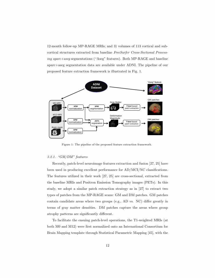
12-month follow-up MP-RAGE MRIs; and 3) volumes of 113 cortical and sub-

cortical structures extracted from baseline FreeSurfer Cross-Sectional Process-

ing aparc+aseg segmentations (“Aseg” features). Both MP-RAGE and baseline

aparc+aseg segmentation data are available under ADNI. The pipeline of our

proposed feature extraction framework is illustrated in Fig. 1.

M0-MRI

SPM

normalization

SPM

normalization

SPM

segmentation

ANTs

registration

Brain maskSPM

normalization

Gray Matter

M12-MRIDeformation Magnitude

GM patches

DM patches

T-test basedpatch extraction

ADNIDataset

“Aseg” feature

T-test basedpatch extraction

Figure 1: The pipeline of the proposed feature extraction framework.

3.2.1. “GM/DM” features

Recently, patch-level neuroimage features extraction and fusion [27, 25] have

been used in producing excellent performance for AD/MCI/NC classifications.

The features utilized in their work [27, 25] are cross-sectional, extracted from

the baseline MRIs and Positron Emission Tomography images (PETs). In this

study, we adopt a similar patch extraction strategy as in [27] to extract two

types of patches from the MP-RAGE scans: GM and DM patches. GM patches

contain candidate areas where two groups (e.g., AD vs. NC) differ greatly in

terms of gray matter densities. DM patches capture the areas where group

atrophy patterns are significantly different.

To facilitate the ensuing patch-level operations, the T1-weighted MRIs (at

both M0 and M12) were first normalized onto an International Consortium for

Brain Mapping template through Statistical Parametric Mapping [45], with the

12

dimensions reduced to 79× 79× 95 and the voxel sizes to 2× 2× 2 mm3. After

spatial normalization, each baseline M0-MRI was segmented into three brain

tissues: GM, WM and CSF. As GM is more related to AD and MCI pathologies

than WM and CSF [25], we choose the GM tissue densities from the baseline

MRIs as the cross-sectional information source in our work. A voxel-wise t-test

was performed for group comparisons of AD vs. NC and MCI vs. NC. Voxels

with statistically significant group difference (with the p-value smaller than 0.05)

were identified as the seeds for patch extraction. The mean p-values in the seed

voxels’ enclosing patches of size 5×5×5 were then used to sort the patch seeds.

Based on their ascending order, we selected the first 100 class-discriminative

patches in a greedy manner with the condition that no candidate patch pair

should have more than 50% overlapping volume. The average GM densities

in these patches form our cross-sectional feature vector, which we call “GM”

feature. Fig. 2 is a visualization of the top 20 GM patches that are selected

from AD vs. NC and MCI vs. NC group comparisons, respectively.

(AD versus NC)

(MCI versus NC)

Figure 2: The top 20 ranked GM patches selected in AD vs. NC and MCI vs. NC group

comparisons. The columns from left to right are sagittal, coronal, axial and 3D views.

13

Our longitudinal DM patches were obtained based on the estimated voxel

deformations matching the baseline and follow-up MRIs for each subject. A dif-

feomorphic registration method provided via ANTs package [46] was utilized to

generate the deformation vector fields. To minimize the effect of the soft-tissue

shifts outside the brains, a dilated MIDAS Whole Brain Mask for each subject

was used to specify the registration area for ANTs. We then calculated the

magnitude (or length) of the deformation vector at each voxel, and a 3D scalar

field of deformation magnitudes (DM) was obtained. Based on the DM scalar

fields, we conducted the same group comparison and patch extraction proce-

dure as for the “GM” features. A set of (top 100 ranked) 3D local patches were

obtained. The average DM values within these patches form our longitudinal

“DM” feature vector. Fig. 3 shows the top 20 DM patches selected from AD

vs. NC and MCI vs. NC group comparisons, respectively.

(AD vs. NC)

(MCI vs. NC)

Figure 3: The top 20 ranked DM patches selected in AD vs. NC and MCI vs. NC group

comparisons. The columns from left to right are sagittal, coronal, axial and 3D views.

14

3.2.2. “Aseg” features

Our “GM” and “DM” features are patch-based. To supplement them with

ROI information, we also include the volumes of brain structures extractable

from FreeSurfer Cross-Sectional Processing aparc+aseg segmentation files, avail-

able under ADNI. The aparc+aseg segmentation files were extracted from MP-

RAGE scans using FreeSurfer [47]. Subcortical structures extracted in aparc+aseg

segmentation [48] include left/right hippocampi, left/right caudate, etc., and

cortical ROI include precuneus, cuneus, etc. Within the FreeSurfer processing

pipeline, all volumetric measurements have been normalized for head size via

dividing by the intracranial volume (ICV). This allows for unbiased compar-

isons between groups at a single time point. In this study, we use 113 volumes

at the baseline visits as another set of features for each subject, which we call

“Aseg” features. The names of the brain structures generated by FreeSurfer

aparc+aseg segmentation can be found in each subjects stats/aseg.stats and

stats/aparc.stats files, as described in https://surfer.nmr.mgh.harvard.edu/

fswiki/FsTutorial/AnatomicalROI. The name list is also included in Ap-

pendix A of this paper. For more information regarding ADNI MRI data anal-

ysis, including FreeSurfer processing, we refer readers to the data hosting site

http://adni.loni.usc.edu/methods/mri-analysis/.

3.3. Feature fusion

The feature extraction steps described above produce 100 features from GM

and DM patches, respectively, and 113 “Aseg” features from “aparc+aseg” seg-

mentation. Inevitably, there should be redundant or irrelevant features in this

set, and the feature dimension, 313, is relatively high for efficient computation.

To approach this high dimensionality problem, the three different types of fea-

tures should be fused with a reduced dimensionality; deep neural network-based

models provide a potentially powerful solution. Deep neural networks have been

utilized in several recent AD/MCI works [23, 30, 27, 49], with the same goal

of learning a latent and compressed representation of the input feature vectors.

Stacked auto-encoder [23, 30], restricted Boltzmann machine [27] and convolu-

15

tional networks [49] are among the choices that have been examined. In this

paper, we adopt a different model — stacked denoising sparse auto-encoder

(stacked DSAE), which is a combination of denoising and sparse auto-encoders

[50, 51]. The “GM/DM/Aseg” features go through stacked DSAE separately,

then we utilize another fusion layer on top to further combine the separate out-

puts. Our approach is different from some recent methods [23, 30]: not only

does it maximize the mutual information from different sources, it also enables

users to control the size of the fused features, desirable for the goal of dimension

reduction.

3.3.1. Stacked denoising sparse auto-encoder (Stacked-DSAE)

The goal of an auto-encoder (AE) is to learn a latent representation for the

input vector x through estimating a nonlinear approximation function hW,b(x) ≈

x. In order to discover interesting structures from the input, certain type of

constraint or regularization needs to be imposed into the network. Sparse auto-

encoder learns sparse over-complete representation by ensuring the majority of

the hidden nodes “inactive” most of the time. This can be done by adding a

sparse penalty into the objective function. Denoising auto-encoder, on the other

hand, obtains a more robust representation by cleaning partially corrupted input

(denoising). In this work, we combine these two models to construct a denoising

sparse auto-encoder (DSAE), and use it as the solution for feature extraction.

This choice is based on the nature of the “GM/DM” features. While easy to

obtain, the “GM/DM” feature vectors contain many non-discriminative compo-

nents. DSAE is designed under the hypothesis that it can learn a compressed

representation from the rather noisy input.

To build a deep network, we stack multiple DSAEs, wiring the outputs of

each hidden layer to the inputs of the successive layer, to form a stacked DSAE.

Such multi-layer networks can be pretrained level by level in a greedy fashion.

Compared with single layer shallow networks, stacked deep networks are more

effective in finding highly nonlinear and complex patterns in data [51]. In this

work, we use three separate stacked DSAEs, for “GM”, “DM”, and “Aseg”

16

features respectively, to extract their latent representations. Similar to the

approach in [27], three hidden layers are used in each stacked DSAE, with the

parameters decided through grid search. More details regarding the parameter

selection will be given in the experimental results section.

3.3.2. Feature fusion through multi-modal stacked DSAE (MM-S-DSAE)

With the latent high level representation discovered by the three stacked

DSAEs for “GM/DM/Aseg” features, the next task is to fuse them without

losing useful information. Ideally, the output dimension should be further de-

creased after the integration, leading to a more compact yet still discriminative

final feature set. Several strategies are available, as shown in Fig. 4. Black and

white circles in this figure represent two different feature types, e.g., “GM” and

“DM”, and gray circles denote the features after fusion. Fig. 4.(b)∼(d) illus-

trate three fusion solutions: (b) shows the most intuitive way that concatenates

different types of feature in the input layer, and learns a single deep neural net-

work, as used in [23]; (c) learns separate deep neural networks for each feature

type, and concatenates the output layers; (d) adds one more fully connected fu-

sion layer on top of (c). In this paper, we choose the last strategy, the so-called

multi-modal stacked DSAE (MM-S-DSAE) as the solution to combine “GM”,

“DM” and “Aseg” features. The advantage of MM-S-DSAE over the other two

alternatives has been empirically validated and will be presented in section 4.3.

…

(a) Stacked DSAE (b) Input concatenation + Stacked DSAE

Input:

…

…Hiddenlayer:

…

Classifier

…

…

…

…

Classifier

… …

(c) Stacked DSAE +Output concatenation

Classifier

…

…

…

…

…

…

…

…

(d) Multi-modal Stacked DSAE

Classifier

…

…

…

…

…

…

…

…

Figure 4: Deep network structures of stacked DSAE (a), and three fusion strategies (b-d).

17

4. Experiments and Results

In this section, we evaluate the proposed TML-SVM metric learning and

MM-S-DSAE feature fusion models through two binary classification problems:

AD vs. NC, and MCI vs. NC. Several experimental setups, including evalu-

ation measures, data partition scheme and the determination of the structure

of our MM-S-DSAE, are explained in section 4.1. We present in section 4.2

the experiments to analyze and compare the discriminative power of individual

feature types and their combinations. In section 4.3, MM-S-DSAE will be evalu-

ated against other feature fusion strategies. Improvements made by TML-SVM

over other classifiers will be examined in section 4.4. Finally, we compare our

method with some recently reported solutions that also use ADNI database for

AD/MCI diagnosis.

4.1. Experimental setups

4.1.1. Performance measures and data partition

Various classification solutions are compared in this section and their perfor-

mance is measured with three evaluation metrics: classification accuracy (ACC),

i.e., the proportion of correctly classified subjects among the whole test set; sen-

sitivity (SEN), i.e., the proportion of correctly classified AD (or MCI) patients;

and specificity (SPE), i.e., the proportion of correctly classified normal controls.

In addition to means and standard deviations, we also report the p-values from

the paired t-test when comparing each performance measure of two different

methods. To ensure a good generalizability for each experiment and compari-

son, we run every experiment 10 times with different random 5-fold splits: three

folds for training, one fold for validation of hyper-parameters, and one fold for

testing.

4.1.2. Determination of the structure of MM-S-DSAE

The topology of MM-S-DSAE is illustrated in Fig. 4.(d). We use three hidden

layers for the underlying stacked DSAE. The numbers of the three layers’ hidden

nodes are selected from [100, 300, 500, 1000] – [50, 100] – [10, 20, 30] (bottom to

18

up). The hyper-parameters for sparsity control and denoising corruption are

both set to 0.2. For the top fusion layer in MM-S-DSAE, the number of hidden

nodes is selected from [3, 5, 8, 10, 15, 20]. The optimal number of hidden nodes

for each layer is determined by the classification performance (accuracy) of the

softmax regression classifier with grid search, similar to [23].

4.1.3. Choice of classifiers

We use softmax regression model in our experiments, with the following

considerations. Being regarded as “the classifier for stacked auto-encoder” [23],

softmax is utilized as the “intuitive” classifier to reduce the potential bias intro-

duced by any particular classifier, which is ideal for comparing the performance

of different features or different fusion strategies. Using softmax as the classifier

also makes “fine-tuning” of stacked DSAE and MM-S-DSAE straightforward.

Due to its popularity, we include softmax as one of the competing algorithms

to evaluate our TML-SVM classifier in section 4.4.

4.2. Comparisons of different features

The first set of experiments is to investigate the efficacy of different features

in distinguishing AD and MCI from normal controls. Specifically, five types

of features, including the aforementioned “GM”, “DM”, “Aseg” features, and

two different combinations of them, i.e, “GM & Aseg” – the combination of

two static cross-sectional features at the baseline visit, “GM & DM & Aseg” –

the combination of both static cross-sectional and longitudinal atrophy features,

are evaluated based on three performance measures, ACC, SEN, and SPE. In

addition, to answer the question if the high level representations learned from

MM-S-DSAE are indeed more discriminative than the original raw features, we

conducted experiments for both “deep” and “raw” versions 2 of the five feature

2In Table 2,“XX (raw)” indicates the results are produced with the original raw features,

and “XX (deep)” are for the features generated through deep neural networks. We use single

modal stacked DSAE to extract “GM (deep)”, “DM (deep)”, “Aseg (deep)”, and MM-S-

DSAE to extract “GM & Aseg (deep)”, “GM & DM & Aseg (deep)”.

19

types. The overall classification results, averaged over 10 runs, are presented in

Table 2.

Table 2: Comparisons of five different features for AD vs. NC and MCI vs. NC classifications.

Boldface denotes the best performance for each measure.

AD versus NC

Classifier Features Hidden nodes 3 ACC(%) SEN(%) SPE(%)

Softmax

GM (raw) —— 77.52 ± 1.91 70.75 ± 3.14 82.67 ± 2.18

GM (deep) 500-100-10 81.44 ± 0.77 75.21 ± 1.35 86.17 ± 1.14

DM (raw) —— 70.23 ± 1.29 66.84 ± 1.34 72.85 ± 2.20

DM (deep) 1000-100-30 79.02 ± 0.93 74.07 ± 0.93 82.83 ± 1.15

Aseg (raw) —— 83.72 ± 1.32 79.53 ± 2.04 86.92 ± 1.74

Aseg (deep) 100-50-30 84.85 ± 1.57 80.82 ± 3.35 87.93 ± 2.07

GM&Aseg (raw) —— 85.21 ± 2.24 80.67 ± 2.46 88.69 ± 2.59

GM&Aseg (deep) · · · -10 86.26 ± 1.53 81.95 ± 2.18 89.56 ± 1.98

GM&DM&Aseg (raw) —— 87.47 ± 1.11 83.63 ± 1.85 90.41 ± 1.72

GM&DM&Aseg (deep) · · · -8 88.73 ± 1.04 84.86 ± 2.08 91.69 ± 1.68

MCI versus NC

Classifier Features Hidden nodes 3 ACC(%) SEN(%) SPE(%)

Softmax

GM (raw) —— 52.49 ± 3.41 53.90 ± 4.86 51.14 ± 3.41

GM (deep) 1000-100-20 75.19 ± 1.36 74.12 ± 2.24 76.31 ± 1.73

DM (raw) —— 55.57 ± 1.99 59.98 ± 3.94 51.21 ± 1.69

DM (deep) 300-100-20 69.97 ± 1.03 64.14 ± 2.23 75.73 ± 0.84

Aseg (raw) —— 53.43 ± 2.33 56.39 ± 2.89 50.48 ± 2.80

Aseg (deep) 1000-100-20 74.30 ± 1.77 73.70 ± 2.27 74.88 ± 3.08

GM&Aseg (raw) —— 53.81 ± 2.35 57.02 ± 2.98 50.67 ± 3.59

GM&Aseg (deep) · · · -15 78.47 ± 2.02 76.76 ± 1.99 80.15 ± 3.17

GM&DM&Aseg (raw) —— 57.10 ± 1.86 58.38 ± 2.47 55.81 ± 2.27

GM&DM&Aseg (deep) · · · -8 80.91 ± 1.53 79.07 ± 2.27 82.70 ± 1.35

From Table 2, it can be observed that the learned “deep” features far out-

perform the corresponding original “raw” features, especially for the MCI vs.

NC classification. The “GM & DM & Aseg” feature is a typical example. The

deep version has significantly better performance 4 than the direct concatena-

tion of the original raw features, “GM & DM & Aseg (raw)”. More specifically,

3For single modal stacked DSAE, we present the optimal number of hidden nodes for each

of three hidden layer (bottom to up); for MM-S-DSAE, we only present the optimal number

of hidden nodes for the last fusion layer, since the previous layers stay the same as in the

single modal ones.4To claim “significantly better” or “significantly improve” in this section, a two-sided p-

20

for AD vs. NC classification, the ACC from “raw” to “deep” has been signif-

icantly improved (p-value = 0.017). For MCI vs. NC classification, all three

performance measures (ACC, SEN, SPE) are significantly improved (p-values

< 0.0001). Furthermore, it is evident that combining longitudinal and baseline

features improves classification performance – the fused “GM & DM & Aseg

(deep)” feature has the highest ACC, SEN and SPE for both AD vs. NC and

MCI vs. NC classifications, with significantly improved performance over the

other four feature types also learned from deep networks, “GM (deep)”, “DM

(deep)”, and “Aseg (deep)”, and “ GM & Aseg (deep)”. For example, the second

best feature type in Table 2, “ GM & Aseg (deep)”, the combination of static

cross-sectional features at the baseline visit, is significantly outperformed by the

“GM & DM & Aseg (deep)” feature for both AD vs. NC (p-values < 0.02) and

MCI vs. NC (p-values < 0.04) classifications.

To further illustrate the role of the proposed dynamic longitudinal feature

(“DM” feature), we conducted another set of comparative experiments that

include static features extracted from 12-month follow-up MRIs, specifically

“GM”, “Aseg” features at 12-month follow-up visits. Those two features were

extracted through a similar pipeline as presented in Section 3, but from the

T1-weighted MP-RAGE MR images at 12-month visits, denoted as “GM-12”,

“Aseg-12”. It would be pointless to spend extra efforts to extract dynamic

longitudinal information between MRIs at baseline and follow-up visits, if there

is no improvement over simply using static cross-sectional features extracted

from the follow-up visits. For this purpose, we compared the performance of

the following two sets of features, “GM” vs. “GM-12” vs. “GM & DM”, and “

GM & Aseg” vs. “GM-12 & Aseg-12” vs. “GM & DM & Aseg ”. In Table 3,

we present the results for those features generated from deep neural networks.

From the results, it can be observed that effort spent on the extraction

of dynamic longitudinal information made a significant difference, especially

value of < 0.05 resulted from “two-sample Student’s t-test” is the criterion for statistical

significance.

21

for the MCI vs. NC classification where brain anatomical changes in MCI

subjects are subtle. Clearly the static features extracted at a later follow-up

visit have more discriminative power than the ones extracted from baseline

visits, especially for AD vs. NC classification. This can be gleaned from the

comparison results of “GM” vs. “GM-12” and “GM & Aseg” vs. “GM-12 &

Aseg-12” in Table 3. However, by integrating dynamic longitudinal information

into static baseline features, the resulted combination generally outperforms

just the static features extracted from follow-up visits for both AD vs. NC, and

MCI vs. NC classifications. Specifically, the fused “GM & DM” feature has

significantly better ACC and SEN measures than static “GM-12” feature for

AD vs. NC classification (p-values < 0.0001) and MCI vs NC classification (p-

values < 0.0001). The trend remains after the ROI feature “Aseg” is included.

“GM & DM & Aseg” still has the highest ACC, SEN and SPE for both AD

vs. NC and MCI vs. NC classifications, with significantly better results in all

three measures (ACC, SEN and SPE) than “GM-12 & Aseg-12” for MCI vs.

NC classification (p-values < 0.04), and slightly better results for AD vs. NC

classification (p-values > 0.05).

Table 3: Comparisons between static and dynamic longitudinal features for AD vs. NC and

MCI vs. NC classifications.

AD versus NC

Classifier Features Hidden nodes ACC(%) SEN(%) SPE(%)

Softmax

GM 500-100-10 81.44 ± 0.77 75.21 ± 1.35 86.17 ± 1.14

GM-12 500-100-20 83.05 ± 0.37 75.97 ± 0.53 88.48 ± 0.36

GM&DM · · · -5 86.92 ± 0.60 86.73 ± 1.59 87.09 ± 0.59

GM&Aseg · · · -10 86.26 ± 1.53 81.95 ± 2.18 89.56 ± 1.98

GM-12&Aseg-12 · · · -3 87.63 ± 1.49 84.25 ± 2.28 90.21 ± 2.42

GM&DM&Aseg · · · -8 88.73 ± 1.04 84.86 ± 2.08 91.69 ± 1.68

MCI versus NC

Classifier Features Hidden nodes ACC(%) SEN(%) SPE(%)

Softmax

GM 1000-100-20 75.19 ± 1.36 74.12 ± 2.24 76.31 ± 1.73

GM-12 500-100-20 75.43 ± 0.60 64.46 ± 0.75 86.26 ± 0.94

GM&DM · · · -10 78.51 ± 1.24 78.61 ± 1.73 78.43 ± 2.39

GM&Aseg · · · -15 78.47 ± 2.02 76.76 ± 1.99 80.15 ± 3.17

GM-12&Aseg-12 · · · -3 78.62 ± 1.57 76.63 ± 1.17 80.59 ± 2.59

GM&DM&Aseg · · · -8 80.91 ± 1.53 79.07 ± 2.27 82.70 ± 1.35

22

4.3. Comparisons of different feature fusion strategies

The second set of experiments is to test the effectiveness of our MM-S-DSAE

design in improving AD/MCI vs. NC classifications, with four other feature fu-

sion strategies compared: 1) concatenation of the original three raw features

(“GM”, “DM”, and “Aseg” features); 2) traditional “PCA based” strategy,

i.e., concatenate the three raw features, and use Principle Component Analysis

(PCA) to reduce the dimension with 99% variances kept; 3) “Input concatena-

tion + Stacked DSAE”, as shown in Fig. 4.(b); and 4) “Stacked DSAE + Output

concatenation”, as shown in Fig. 4.(c). We adopt the same performance mea-

sures (ACC, SEN, SPE) and experimental setting (5-fold splits with 10 runs),

and use softmax regression classifier as in Section 4.2. The classification results

of each strategy for AD/MCI vs. NC are summarized in Table 4.

Table 4: Five feature fusion strategies for AD vs. NC and MCI vs. NC classifications.

AD versus NC

Classifier Feature Hidden nodes 5 ACC(%) SEN(%) SPE(%)

Softmax

Direct concatenation —– 87.47 ± 1.11 83.63 ± 1.85 90.41 ± 1.72

PCA based —– 86.12 ± 0.97 81.88 ± 2.30 89.34 ± 1.25

Input concat. + S-DSAE 1000-500-10 87.92 ± 1.50 86.30 ± 3.24 89.17 ± 1.28

S-DSAE + Output concat. · · · -70 87.46 ± 1.09 82.54 ± 1.89 91.20 ± 2.17

MM-S-DSAE · · · -8 88.73 ± 1.04 84.86 ± 2.08 91.69 ± 1.68

MCI versus NC

Classifier Feature Hidden nodes ACC(%) SEN(%) SPE(%)

Softmax

Direct concatenation —– 57.10 ± 1.86 58.38 ± 2.47 55.81 ± 2.27

PCA based —– 53.73 ± 2.51 54.69 ± 2.30 52.78 ± 3.58

Input concat. + S-DSAE 1000-50-20 80.33 ± 2.20 78.42 ± 3.27 82.19 ± 2.02

S-DSAE + Output concat. · · · -60 80.16 ± 0.80 75.86 ± 1.42 84.37 ± 0.76

Multi-modal S-DSAE · · · -8 80.91 ± 1.53 79.07 ± 2.27 82.70 ± 1.35

As we can see from the results, the adopted MM-S-DSAE has the best overall

classification performance: it produces the highest ACC, SPE for AD vs. NC

5For “input concat. + S-DSAE” fusion strategy, we present the optimal number of hidden

nodes for each of three hidden layer (bottom to up); for “S-DSAE + Output concat.” and

MM-S-DSAE fusion strategies, we only present the number of hidden nodes for the last con-

catenation or fusion layer, since the previous layers stay the same as in single modal stacked

DSAE.

23

classification and the highest ACC, SEN for MCI vs. NC classification. While

not surpassing the other two deep fusion strategies in all measures, the MM-S-

DSAE does learn a much more compact high level feature representation than

the other two deep fusion strategies, with better or comparable classification

performance. Specifically, for “Input concatenation + Stacked DSAE” strategy,

the optimal node size of the output layer is 10 in AD vs. NC classification, and

20 in MCI vs. NC classification; for “Stacked DSAE + Output concatenation”

strategy, the optimal node size of the output concatenation layer is 70 in AD

vs. NC classification, and 60 in MCI vs. NC classification; for MM-S-DSAE

strategy, the optimal node size of the output fusion layer is 8 in both AD vs.

NC and MCI vs. NC classifications. Compared to the original raw feature

dimension (313), our MM-S-DSAE was able to achieve 97.5% feature dimension

reduction.

4.4. Comparisons of TML-SVM with other classifiers

The last set of experiments seeks to test the effectiveness of the nonlinear

feature transformation introduced by our proposed TML-SVM classifier in im-

proving AD/MCI vs. NC classifications. We compare TML-SVM against two

other classifiers without feature transformation: softmax regression and tradi-

tional SVM. For all the three classifiers, the same MM-S-DSAE model is used to

obtain the fused feature representations. It is worth noting that only the deep

network in softmax regression model is fine-tuned. For SVM, the slackness coef-

ficient C is selected from {2−5 ∼ 215}. TML-SVM has three hyper-parameters

to be tuned: the number of anchor points p and the tradeoff coefficients C1 and

C2. For p, we empirically set it to 30% of the training samples; for C1 and

C2, we select them from {2−5 ∼ 215} and {5−5 ∼ 525} respectively. We still

adopt the same experimental setting and performance measures, and report the

results averaged from 10 runs in Table 5.

As evident, our TML-SVM has the best classification performance with the

highest ACC, SEN, SPE for both AD vs. NC and MCI vs. NC classifications.

In particular, the improvements made by TML-SVM over the host classifier

24

Table 5: Comparisons of three different classifiers for AD vs. NC and MCI vs. NC classifica-

tions.AD versus NC(%) MCI versus NC(%)

Classifier ACC(%) SEN(%) SPE(%) ACC(%) SEN(%) SPE(%)

Softmax 88.73 ± 1.04 84.86 ± 2.08 91.69 ± 1.68 80.91 ± 1.53 79.07 ± 2.27 82.70 ± 1.35

SVM 89.50 ± 0.86 87.16 ± 1.97 91.27 ± 1.02 80.52 ± 1.24 80.13 ± 2.58 80.93 ± 1.71

TML-SVM 91.95 ± 1.00 89.49 ± 2.37 93.82 ± 1.63 83.72 ± 1.16 84.74 ± 2.34 82.72 ± 1.19

SVM are significant (for AD vs. NC, p-values < 0.03; for MCI vs. NC, p-values

< 0.02), which means adding the nonlinear feature transformation is effective

in making the mapped data points more linearly separable. Also, we note that

the deep neural networks used in SVM and TML-SVM are not fine-tuned as in

softmax regression model, thus we believe the performance of our TML-SVM

can be further improved if fine-tuning is utilized.

4.5. Comparisons with state-of-the-art AD staging methods

Numerous solutions [27, 28, 29, 25, 30, 31, 32] have been proposed in the

literature for AD/MCI patient classification. Some very recent works [27, 30]

reported rather high accuracies through the applications of multi-modality infor-

mation integration (mainly MRIs and PETs) and sophisticated multi-classifier

decision fusion schemes. Analysis of the solutions striving to address the same

problem is crucial to advance the developments of highly effective methods.

However, direct comparisons of the published neuroimaging algorithms are of-

ten not feasible, unless common subjects, datasets and modalities are employed,

as in the evaluation project conducted by Cuingnet et al. [28]. When differ-

ent datasets and experimental setups are utilized, which is common for many

neuroimage studies, higher accuracy or better results over a competing solution

ought to be interpreted as indirect evidence of the model efficacy, rather than

the proof of superiority for head-to-head competitions.

We conduct the first set of comparisons with the solutions that are very

close to our model in nature. Four recently published works are chosen: 1)

voxel-wise GM densities based method by Kloppel et al. [21] which obtained

the best performance among the ten methods evaluated in [28]; 2) 93-region

25

GM densities method by Zhang et al. [29], 3) the single classifier results using

patch-wise GM, as presented in Liu et al. [25], and 4) a longitudinal work by

McEvoy et al. [34], which uses the quadratic discriminant analyses (QDAs) as

the classifier with ROI features extracted from the baseline and one-year follow-

up information. Unlike the “DM” features in our work, the subtraction-based

atrophy calculation in [34] is not dynamic. Similar to our method, these four

solutions all use MR images as the sole information source and rely on single

classifiers for classification. The comparison results are shown in Table 6.

Table 6: Comparisons of our proposed method with other existing methods for AD vs. NC

and MCI vs. NC classifications within the same category.

Method Study Feature Classifier AD versus NC MCI versus NC

Size ACC(%) SEN(%) SPE(%) ACC(%) SEN(%) SPE(%)

Cuingnet et al.[28] 475 Voxel-wise GM SVM 88.6 81.0 95.0 81.2 73.0 85.0

Zhang et al.[29] 202 93 ROI GMs SVM 86.2 86.0 86.3 72.0 78.5 59.6

Liu et al.[25] 652 Patch-wise GM SVM 86.4 83.9 88.6 79.4 79.2 79.5

McEvoy et al. [34] 684 8 ROI volumes QDAs 90.8 91.3 90.5 — — —

Proposed 338 Fused G/D/A TML-SVM 91.95 89.49 93.82 83.72 84.74 82.72

From Table 6, we make the following observations. Our proposed model

performs better than the competing methods in terms of classification accuracy

in AD vs. NC classification, and accuracy and sensitivity in MCI vs. NC

classification. Although the results for specificity reported in [28] are slightly

higher than ours, it is at the expense of sacrificing sensitivity, leading to a

worse accuracy. Researchers in [34] reported the highest sensitivity for AD vs.

NC classification, but their accuracy and specificity are relatively lower than

those produced in our method. In addition, compared to those three methods

[28, 29, 25] that only use cross-sectional information at the baseline visits, our

method achieves consistently better accuracy and sensitivity in both AD vs. NC

and MCI vs. NC classifications. It is worth noting that high sensitivity may

be advantageous for confident AD diagnosis at early stage, which is potentially

useful in clinical practice.

In addition, we compare our model with six works that have reported very

high, if not the highest, classification rates for AD/MCI vs. NC. The results

26

are shown in Table 7. Five of them use cross-sectional information. The works

of Suk et al. [27] and Liu et al. [30] are built on deep neural networks, and

their high performance should not be a surprise as they both utilize PET as an

additional feature source. The single-classifier version of Liu et al. [25] shown

in Table 6 is outperformed by our model, but their multi-SVM version, through

sophisticated multi-classifier decision fusion schemes, produces significantly im-

proved results. Liu et al. [31, 32] use multiple templates and combine the

outputs from multiple SVMs to achieve impressively high accuracies. Li et al.

[33] use multi-year longitudinal information, including scans from 36-month vis-

its, in their solution. As AD patients’ late scans are commonly more revealing

than those at baseline, very accurate diagnosis (96.1%) becomes possible.

While our model is single-classifier based, it achieves comparable perfor-

mance with some of the aforementioned multi-classifier solutions. Upgrading

our TPS-SVM with multi-kernel or multiple SVMs, or applying metric learning

to the solutions in Table 7, could both potentially lead to performance improve-

ments for the respective models. Structure MRIs are the sole information source

of our current solution, therefore it can be expected that the performance of our

model can be further improved if additional modalities, e.g., PET, functional

MRI or diffusion tensor imaging (DTI), are integrated as inputs. All in all, we

believe our pipeline achieves rather high accuracy in AD/MCI vs. NC classi-

fication with simple setups and limited information sources (structural MRIs

alone), and lays a solid foundation for further integration and generalization.

Table 7: Comparisons of the proposed TML-SVM with state-of-the-art methods for AD vs.

NC and MCI vs. NC classifications.Method Study Modality Classifier AD versus NC MCI versus NC

Size ACC(%) SEN(%) SPE(%) ACC(%) SEN(%) SPE(%)

Liu et al.[25] 652 MRI Hierarchical fusion 92.0 90.9 93.0 85.3 82.3 88.2

Suk et al.[27] 398 MRI + PET Deep Boltzmann machine 95.4 94.7 95.2 85.7 95.4 65.9

Liu et al.[30] 331 MRI + PET Stacked parse auto-encoder 91.4 92.3 90.4 82.1 60.0 92.3

Liu et al.[31] 331 MRI SVM ensemble 92.51 92.89 88.3 — — —

Liu et al.[32] 331 MRI SVM ensemble 93.06 94.85 90.49 — — —

Li et al.[33] 152 MRI SVM 96.1 — — — — —

Proposed 338 MRI TML-SVM 91.95 89.49 93.82 83.72 84.74 82.72

27

5. Discussions and Conclusions

This study is designed with two major goals: 1) to develop a nonlinear

metric learning solution and to explore if AD/MCI diagnosis can benefit from

it; and 2) exploring how cross-sectional (baseline) and longitudinal (atrophy

rates) information can be effectively integrated.

Metric learning has been an active research area in machine learning for

more than a decade, but its ability to improve supervised and semi-supervised

classification has not been fully recognized in neuroimaging community. Our

TML-SVM model learns a globally smooth deformation for the input space,

and it is the first work that utilizes nonlinear dense transformations, or spa-

tially varying deformation models in metric learning. Using the ADNI dataset,

we evaluated the effectiveness of our TML-SVM mode in improving AD/MCI di-

agnosis, and we hope a take-home message will be delivered to the neuroimaging

community: metric learning does help.

Our proposed MM-S-DASE model is a deep learning solution to extract

latent, high-level integrated feature representation from three raw features ob-

tained through conventional feature engineering pipeline often used for statis-

tical analysis and segmentation. Although deep learning methods are proven

for automatically extracting meaningful representation from raw images, trans-

planting them to neuroimaging applications is often not trivial. Firstly, neu-

roimages are commonly high-resolution 3D images, tens or hundreds times larger

than photographic 2D images. This creates much higher dimensional inputs if

the volumetric images are used directly. Secondly, deep learning works best

with large numbers of training samples, which are typically unavailable for indi-

vidual clinical trials and human subject studies. These two factors significantly

restrict the power of deep learning in neuroimaging applications. Patch features

and patch-based learning, in our opinion, provide a remedy for both issues,

and therefore can help bridge the research gap between computer vision and

neuroimage analysis. Further efforts to explore patch-based solutions in neu-

roimaging appear warranted.

28

As multimodality images can provide complementary information in disease

diagnoses, combining different modalities will likely lead to more accurate deci-

sion boundaries. The high accuracies reported in [27, 23] support this notion.

Vast amounts of imaging and other data are collected on patients every day as

part of standard medical care, yet virtually none of it is aggregated, processed

and extracted using deep learning and related methods to support physician de-

cision making at the present time. The exciting long term potential for this role

should be clear just from the example of research we have presented here. But

research requires focus. In the future work, we will explore features from other

data modalities, including PET, fMRI, DTI, and genetic data. Enhancing our

TML-SVM with multi-kernelization, as well as exploring other geometric models

than TPS, are among the directions of our ongoing efforts.

6. Acknowledgments

This study was financially supported by grants by Stocker Endowment,

Moores Alzheimer Research Endowment, Sanders-Brown Center on Aging and

University of Kentucky College of Medicine.

Data collection and sharing for this project was funded by the Alzheimer’s

Disease Neuroimaging Initiative (ADNI) (National Institutes of Health Grant

U01 AG024904) and DOD ADNI (Department of Defense award number W81XWH-

12-2-0012). ADNI is funded by the National Institute on Aging, the National In-

stitute of Biomedical Imaging and Bioengineering, and through generous contri-

butions from the following: AbbVie, Alzheimers Association; Alzheimers Drug

Discovery Foundation; Araclon Biotech; BioClinica, Inc.; Biogen; Bristol-Myers

Squibb Company; CereSpir, Inc.; Eisai Inc.; Elan Pharmaceuticals, Inc.; Eli

Lilly and Company; EuroImmun; F. Hoffmann-La Roche Ltd and its affili-

ated company Genentech, Inc.; Fujirebio; GE Healthcare; IXICO Ltd.; Janssen

Alzheimer Immunotherapy Research & Development, LLC.; Johnson & Johnson

Pharmaceutical Research & Development LLC.; Lumosity; Lundbeck; Merck &

Co., Inc.; Meso Scale Diagnostics, LLC.; NeuroRx Research; Neurotrack Tech-

29

nologies; Novartis Pharmaceuticals Corporation; Pfizer Inc.; Piramal Imaging;

Servier; Takeda Pharmaceutical Company; and Transition Therapeutics. The

Canadian Institutes of Health Research is providing funds to support ADNI

clinical sites in Canada. Private sector contributions are facilitated by the

Foundation for the National Institutes of Health (www.fnih.org). The grantee

organization is the Northern California Institute for Research and Education,

and the study is coordinated by the Alzheimer’s Disease Cooperative Study at

the University of California, San Diego. ADNI data are disseminated by the

Laboratory for Neuro Imaging at the University of Southern California.

7. Appendix: Names of the 113 anatomical structures in Aseg fea-

tures

The Aseg feature set in this study consists of the volumes of 113 cortical

and subcortical brain structures extracted from the FreeSurfer Cross-Sectional

Processing aparc+aseg segmentation files, available under ADNI. These struc-

tures were segmented from the subjects’ T1-weighted MRI scans. All features

have been normalized by the corresponding whole brain volumes. The list of the

structure names is provided as follows. Aseg list contains subcortical structures,

and Aparc is for cortical structures.

Aseg structures Left-Lateral-Ventricle, Left-Inf-Lat-Vent, Left-Cerebellum-White-

Matter, Left-Cerebellum-Cortex, Left-Thalamus-Proper, Left-Caudate, Left-

Putamen, Left-Pallidum, 3rd-Ventricle, 4th-Ventricle, Brain-Stem, Left-

Hippocampus, Left-Amygdala, CSF, Left-Accumbens-area, Left-VentralDC,

Left-vessel, Left-choroid-plexus, Right-Lateral-Ventricle, Right-Inf-Lat-Vent,

Right-Cerebellum-White-Matter, Right-Cerebellum-Cortex, Right-Thalamus-

Proper, Right-Caudate, Right-Putamen, Right-Pallidum, Right-Hippocampus,

Right-Amygdala, Right-Accumbens-area, Right-VentralDC, Right-vessel,

Right-choroid-plexus, 5th-Ventricle, WM-hypointensities, Left-WM-hypointensities,

Right-WM-hypointensities, non-WM-hypointensities, Left-non-WM-hypointensities,

30

Right-non-WM-hypointensities, Optic-Chiasm, CC-Posterior, CC-Mid-Posterior,

CC-Central, CC-Mid-Anterior, CC-Anterior.

Aparc structures ctx-lh-bankssts, ctx-lh-caudalanteriorcingulate, ctx-lh-caudalmiddlefrontal,

ctx-lh-cuneus, ctx-lh-entorhinal, ctx-lh-fusiform, ctx-lh-inferiorparietal, ctx-

lh-inferiortemporal, ctx-lh-isthmuscingulate, ctx-lh-lateraloccipital, ctx-

lh-lateralorbitofrontal, ctx-lh-lingual, ctx-lh-medialorbitofrontal, ctx-lh-middletemporal,

ctx-lh-parahippocampal, ctx-lh-paracentral, ctx-lh-parsopercularis, ctx-lh-

parsorbitalis, ctx-lh-parstriangularis, ctx-lh-pericalcarine, ctx-lh-postcentral,

ctx-lh-posteriorcingulate, ctx-lh-precentral, ctx-lh-precuneus, ctx-lh-rostralanteriorcingulate,

ctx-lh-rostralmiddlefrontal, ctx-lh-superiorfrontal, ctx-lh-superiorparietal,

ctx-lh-superiortemporal, ctx-lh-supramarginal, ctx-lh-frontalpole, ctx-lh-

temporalpole, ctx-lh-transversetemporal, ctx-lh-insula, ctx-rh-bankssts, ctx-

rh-caudalanteriorcingulate, ctx-rh-caudalmiddlefrontal, ctx-rh-cuneus, ctx-

rh-entorhinal, ctx-rh-fusiform, ctx-rh-inferiorparietal, ctx-rh-inferiortemporal,

ctx-rh-isthmuscingulate, ctx-rh-lateraloccipital, ctx-rh-lateralorbitofrontal,

ctx-rh-lingual, ctx-rh-medialorbitofrontal, ctx-rh-middletemporal, ctx-rh-

parahippocampal, ctx-rh-paracentral, ctx-rh-parsopercularis, ctx-rh-parsorbitalis,

ctx-rh-parstriangularis, ctx-rh-pericalcarine, ctx-rh-postcentral, ctx-rh-posteriorcingulate,

ctx-rh-precentral, ctx-rh-precuneus, ctx-rh-rostralanteriorcingulate, ctx-

rh-rostralmiddlefrontal, ctx-rh-superiorfrontal, ctx-rh-superiorparietal, ctx-

rh-superiortemporal, ctx-rh-supramarginal, ctx-rh-frontalpole, ctx-rh-temporalpole,

ctx-rh-transversetemporal, ctx-rh-insula.

8. References

[1] A. Alzheimers, 2015 Alzheimer’s disease facts and figures., Alzheimer’s &

dementia: the journal of the Alzheimer’s Association 11 (3) (2015) 332.

[2] A. J. Mitchell, M. Shiri-Feshki, Rate of progression of mild cognitive im-

pairment to dementia–meta-analysis of 41 robust inception cohort studies,

Acta Psychiatrica Scandinavica 119 (4) (2009) 252–265.

31

[3] I. A. van Rossum, S. J. Vos, L. Burns, D. L. Knol, P. Scheltens, H. Soininen,

L.-O. Wahlund, H. Hampel, M. Tsolaki, L. Minthon, et al., Injury markers

predict time to dementia in subjects with MCI and amyloid pathology,

Neurology 79 (17) (2012) 1809–1816.

[4] C. R. Jack, et al., The Alzheimer’s disease neuroimaging initiative (ADNI):

MRI methods, Journal of Magnetic Resonance Imaging 27 (4) (2008) 685–

691.

[5] A. Bellet, A. Habrard, M. Sebban, A survey on metric learning for feature

vectors and structured data, arXiv preprint arXiv:1306.6709.

[6] L. Yang, R. Jin, Distance metric learning: A comprehensive survey, Michi-

gan State Universiy 2 (2006) 78.

[7] E. P. Xing, A. Y. Ng, M. I. Jordan, S. Russell, Distance metric learning

with application to clustering with side-information, Advances in neural

information processing systems 15 (2003) 505–512.

[8] J. Goldberger, G. E. Hinton, S. T. Roweis, R. Salakhutdinov, Neighbour-

hood components analysis, Advances in neural information processing sys-

tems (2004) 513–520.

[9] M. Schultz, T. Joachims, Learning a distance metric from relative compar-

isons, Advances in neural information processing systems (2004) 41.

[10] J. V. Davis, B. Kulis, P. Jain, S. Sra, I. S. Dhillon, Information-theoretic

metric learning, in: Proceedings of the 24th international conference on

Machine learning, ACM, 2007, pp. 209–216.

[11] K. Q. Weinberger, J. Blitzer, L. K. Saul, Distance metric learning for large

margin nearest neighbor classification, Advances in Neural Information

Processing Systems (2005) 1473–1480.

[12] A. Globerson, S. Roweis, Metric learning by collapsing classes, Advances

in neural information processing systems (2005) 451–458.

32

[13] L. Torresani, K.-c. Lee, Large margin component analysis, Advances in

neural information processing systems 19 (2007) 1385.

[14] J. T. Kwok, I. W. Tsang, Learning with idealized kernels, Proceedings of

the Twentieth International Conference on Machine Learning (ICML-03)

(2003) 400–407.

[15] R. Chatpatanasiri, T. Korsrilabutr, P. Tangchanachaianan, B. Kijsirikul, A

new kernelization framework for Mahalanobis distance learning algorithms,

Neurocomputing 73 (10) (2010) 1570–1579.

[16] K. Q. Weinberger, L. K. Saul, Distance metric learning for large margin

nearest neighbor classification, The Journal of Machine Learning Research

10 (2009) 207–244.

[17] Y. Hong, Q. Li, J. Jiang, Z. Tu, Learning a mixture of sparse distance met-

rics for classification and dimensionality reduction, in: 2011 International

Conference on Computer Vision, IEEE, 2011, pp. 906–913.

[18] D. Ramanan, S. Baker, Local distance functions: A taxonomy, new algo-

rithms, and an evaluation, IEEE Trans. Pattern Anal. Mach. Intell. 33 (4)

(2011) 794–806.

[19] Y.-K. Noh, B.-T. Zhang, D. D. Lee, Generative local metric learning for

nearest neighbor classification, in: Advances in Neural Information Pro-

cessing Systems, 2010, pp. 1822–1830.

[20] J. Wang, A. Kalousis, A. Woznica, Parametric local metric learning for

nearest neighbor classification, in: Advances in Neural Information Pro-

cessing Systems, 2012, pp. 1601–1609.

[21] S. Kloppel, et al., Automatic classification of MR scans in Alzheimer’s

disease, Brain 131 (3) (2008) 681–689.

[22] M. Chupin, A. Hammers, R. S. Liu, O. Colliot, J. Burdett, E. Bardinet,

J. S. Duncan, L. Garnero, L. Lemieux, Automatic segmentation of the

33

hippocampus and the amygdala driven by hybrid constraints: method and

validation, Neuroimage 46 (3) (2009) 749–761.

[23] H.-I. Suk, S.-W. Lee, D. Shen, A. D. N. Initiative, et al., Latent feature rep-

resentation with stacked auto-encoder for AD/MCI diagnosis, Brain Struc-

ture and Function 220 (2) (2015) 841–859.

[24] Y. Fan, D. Shen, R. C. Gur, R. E. Gur, C. Davatzikos, Compare: classi-

fication of morphological patterns using adaptive regional elements, IEEE

transactions on medical imaging 26 (1) (2007) 93–105.

[25] M. Liu, D. Zhang, D. Shen, Hierarchical fusion of features and classifier

decisions for Alzheimer’s disease diagnosis, Human brain mapping 35 (4)

(2014) 1305–1319.

[26] G. Wu, M. Kim, G. Sanroma, Q. Wang, B. C. Munsell, D. Shen, A. D. N.

Initiative, et al., Hierarchical multi-atlas label fusion with multi-scale fea-

ture representation and label-specific patch partition, NeuroImage 106

(2015) 34–46.

[27] H.-I. Suk, S.-W. Lee, D. Shen, A. D. N. Initiative, et al., Hierarchical fea-

ture representation and multimodal fusion with deep learning for AD/MCI

diagnosis, NeuroImage 101 (2014) 569 – 582.

[28] R. Cuingnet, E. Gerardin, J. Tessieras, G. Auzias, S. Lehericy, M.-O.

Habert, M. Chupin, H. Benali, O. Colliot, A. D. N. Initiative, et al., Au-

tomatic classification of patients with Alzheimer’s disease from structural

MRI: a comparison of ten methods using the ADNI database, neuroimage

56 (2) (2011) 766–781.

[29] D. Zhang, Y. Wang, L. Zhou, H. Yuan, D. Shen, A. D. N. Initiative, et al.,

Multimodal classification of Alzheimer’s disease and mild cognitive impair-

ment, Neuroimage 55 (3) (2011) 856–867.

[30] S. Liu, S. Liu, W. Cai, H. Che, S. Pujol, R. Kikinis, D. Feng, M. J. Fulham,

et al., Multimodal Neuroimaging Feature Learning for Multiclass Diagno-

34

sis of Alzheimer’s Disease, IEEE Transactions on Biomedical Engineering

62 (4) (2015) 1132–1140.

[31] M. Liu, D. Zhang, D. Shen, View-centralized multi-atlas classification for

Alzheimer’s disease diagnosis, Human brain mapping 36 (5) (2015) 1847–

1865.

[32] M. Liu, D. Zhang, D. Shen, Relationship induced multi-template learning

for diagnosis of Alzheimers disease and mild cognitive impairment, IEEE

transactions on medical imaging 35 (6) (2016) 1463–1474.

[33] Y. Li, Y. Wang, G. Wu, F. Shi, L. Zhou, W. Lin, D. Shen, Alzheimer’s

Disease Neuroimaging Initiative, et al., Discriminant analysis of longitu-

dinal cortical thickness changes in Alzheimer’s disease using dynamic and

network features, Neurobiology of aging 33 (2) (2012) 427–e15.

[34] L. K. McEvoy, D. Holland, D. J. Hagler Jr, C. Fennema-Notestine, J. B.

Brewer, A. M. Dale, Mild cognitive impairment: baseline and longitudinal

structural MR imaging measures improve predictive prognosis, Radiology

259 (3) (2011) 834–843.

[35] B. jie, M. Liu, J. Liu, D. Zhang, D. Shen, Temporally-constrained group

sparse learning for longitudinal data analysis in Alzheimer’s disease, IEEE

Transactions on Biomedical Engineering PP (99) (2016) 1–1. doi:10.1109/

TBME.2016.2553663.

[36] H.-I. Suk, S.-W. Lee, D. Shen, A hybrid of deep network and hidden markov

model for MCI identification with resting-state fMRI, in: International

Conference on Medical Image Computing and Computer-Assisted Inter-

vention, Springer, 2015, pp. 573–580.

[37] Z. Xu, K. Q. Weinberger, O. Chapelle, Distance metric learning for kernel

machines, arXiv preprint arXiv:1208.3422.

35

[38] X. Zhu, P. Gong, Z. Zhao, C. Zhang, Learning similarity metric with SVM,

in: The 2012 International Joint Conference on Neural Networks (IJCNN),

IEEE, 2012, pp. 1–8.

[39] G. Wahba, Spline models for observational data, Vol. 59, Siam, 1990.

[40] J. Duchon, Splines minimizing rotation-invariant semi-norms in Sobolev

spaces, in: Constructive theory of functions of several variables, Springer,

1977, pp. 85–100.

[41] H. Chui, A. Rangarajan, A new point matching algorithm for non-rigid

registration, Computer Vision and Image Understanding 89 (2) (2003) 114–

141.

[42] L. Kaufman, P. Rousseeuw, Clustering by means of medoids, North-

Holland, 1987.

[43] H.-S. Park, C.-H. Jun, A simple and fast algorithm for k-medoids clustering,

Expert Systems with Applications 36 (2) (2009) 3336–3341.

[44] H. Do, A. Kalousis, M. Hilario, Feature weighting using margin and radius

based error bound optimization in svms, in: Joint European Conference on

Machine Learning and Knowledge Discovery in Databases, Springer, 2009,

pp. 315–329.

[45] A. Mechelli, C. J. Price, K. J. Friston, J. Ashburner, Voxel-based mor-

phometry of the human brain: methods and applications, Current Medical

Imaging Reviews 1 (2) (2005) 105–113.

[46] B. B. Avants, N. Tustison, G. Song, Advanced normalization tools (ANTS),

Insight J (2009) 1–35.

[47] B. Fischl, Freesurfer, Neuroimage 62 (2) (2012) 774–781.

[48] B. Fischl, D. H. Salat, E. Busa, M. Albert, M. Dieterich, C. Haselgrove,

A. Van Der Kouwe, R. Killiany, D. Kennedy, S. Klaveness, et al., Whole

36

brain segmentation: automated labeling of neuroanatomical structures in

the human brain, Neuron 33 (3) (2002) 341–355.

[49] A. Gupta, M. Ayhan, A. Maida, Natural image bases to represent neu-

roimaging data, in: Proceedings of the 30th International Conference on

Machine Learning (ICML-13), Vol. 28, JMLR Workshop and Conference

Proceedings, 2013, pp. 987–994.

URL http://jmlr.org/proceedings/papers/v28/gupta13b.pdf

[50] P. Vincent, H. Larochelle, Y. Bengio, P.-A. Manzagol, Extracting and com-

posing robust features with denoising autoencoders, in: Proceedings of the

25th international conference on Machine learning, ACM, 2008, pp. 1096–

1103.

[51] Y. Bengio, Learning deep architectures for AI, Foundations and trends R©

in Machine Learning 2 (1) (2009) 1–127.

37