
Nonlinear dynamics and breakup of free-surface flowsunix12.fzu.cz/~vybornyk/25/p865_1.pdf ·...
65
Nonlinear dynamics and breakup of free-surface flows Jens Eggers Universita ¨ t Gesamthochschule Essen, Fachbereich Physik, 45117 Essen, Germany Surface-tension-driven flows and, in particular, their tendency to decay spontaneously into drops have long fascinated naturalists, the earliest systematic experiments dating back to the beginning of the 19th century. Linear stability theory governs the onset of breakup and was developed by Rayleigh, Plateau, and Maxwell. However, only recently has attention turned to the nonlinear behavior in the vicinity of the singular point where a drop separates. The increased attention is due to a number of recent and increasingly refined experiments, as well as to a host of technological applications, ranging from printing to mixing and fiber spinning. The description of drop separation becomes possible because jet motion turns out to be effectively governed by one-dimensional equations, which still contain most of the richness of the original dynamics. In addition, an attraction for physicists lies in the fact that the separation singularity is governed by universal scaling laws, which constitute an asymptotic solution of the Navier-Stokes equation before and after breakup. The Navier-Stokes equation is thus continued uniquely through the singularity. At high viscosities, a series of noise-driven instabilities has been observed, which are a nested superposition of singularities of the same universal form. At low viscosities, there is rich scaling behavior in addition to aesthetically pleasing breakup patterns driven by capillary waves. The author reviews the theoretical development of this field alongside recent experimental work, and outlines unsolved problems. [S0034-6861(97)00303-6] CONTENTS I. Introduction 865 II. Experiments 869 A. Jet 869 B. Dripping faucet 872 C. Liquid bridge 873 III. Simulations 874 A. Inviscid, irrotational flow 875 B. Stokes flow 876 C. Navier-Stokes simulations 877 IV. Small Perturbations 878 A. Linear stability 878 B. Spatial instability 882 C. Higher-order perturbative analysis 883 V. One-Dimensional Approximations 885 A. Radial expansion method 886 B. Averaging method: Cosserat equations 888 C. Basic properties and simulations 889 D. Inviscid theory and conservation laws 892 VI. Similarity Solutions and Breakup 894 A. Local similarity form 894 B. Before breakup 895 C. Stability and the influence of noise 897 D. After breakup 900 VII. Away From Breakup 904 A. High viscosity—threads 904 B. Low viscosity—cones 907 C. Satellite drops 911 VIII. Related Problems 914 A. Two-fluid systems 914 1. Stationary shapes 915 2. Breakup 917 B. Electrically driven jets 919 C. Polymeric liquids 922 IX. Outlook 924 Acknowledgments 925 References 926 I. INTRODUCTION The formation of drops is a phenomenon ubiquitous in daily life, science, and technology. But although it is plain that drops generically result from the motion of free surfaces, it is not easy to predict the distribution of their sizes or to observe the intricate dynamics involved; see Fig. 1. Only the extremely short flash used by the photographer, Harold Edgerton, clearly reveals the for- mation of individual drops. Thus the subject has been far from exhausted after more than 300 years of scien- tific research, which in fact has gained considerable mo- mentum only recently. On the one hand, the reason for this interest lies in the tremendous technological impor- tance of drop formation in mixing, spraying, and chemi- cal processing, which leads to applications such as ink-jet printing, fiber spinning, and silicon chip technology. On the other hand, the modern theory of nonlinear phe- nomena has created a new paradigm of self-similarity and scaling, which opened a new perspective on this classical problem. The first mention of drop formation in the scientific literature is in a book by Mariotte (1686) on the motion of fluids. He notes that a stream of water flowing from a hole in the bottom of a container decays into drops. Like many authors after him, he assumes that gravity, or other external forces, are responsible for the process. A simple estimate shows, however, that uniform forces cannot lead to drop formation and that another force, which of course is surface tension, is responsible for the eventual breakoff of drops. For reasons of mass conser- vation, the rate at which the minimal cross section of a fluid filament decreases is proportional to the cross sec- tion itself, multiplied by an axial velocity gradient. As long as this gradient is finite, as is to be expected when only uniform forces are acting, the decrease of the mini- mum thickness will be at most exponential, leading to separation only in infinite time. The basis for a more thorough understanding of drop formation was laid by Savart (1833), who very carefully investigated the decay of fluid jets. By illuminating the jet with sheets of light, he observed tiny undulations growing on a jet of water, as shown in Fig. 2. These 865 Reviews of Modern Physics, Vol. 69, No. 3, July 1997 0034-6861/97/69(3)/865(65)/$19.75 © 1997 The American Physical Society
Transcript of Nonlinear dynamics and breakup of free-surface flowsunix12.fzu.cz/~vybornyk/25/p865_1.pdf ·...

Nonlinear dynamics and breakup of free-surface flows
Jens Eggers
Universitat Gesamthochschule Essen, Fachbereich Physik, 45117 Essen, Germany
Surface-tension-driven flows and, in particular, their tendency to decay spontaneously into drops havelong fascinated naturalists, the earliest systematic experiments dating back to the beginning of the 19thcentury. Linear stability theory governs the onset of breakup and was developed by Rayleigh, Plateau,and Maxwell. However, only recently has attention turned to the nonlinear behavior in the vicinity ofthe singular point where a drop separates. The increased attention is due to a number of recent andincreasingly refined experiments, as well as to a host of technological applications, ranging fromprinting to mixing and fiber spinning. The description of drop separation becomes possible because jetmotion turns out to be effectively governed by one-dimensional equations, which still contain most ofthe richness of the original dynamics. In addition, an attraction for physicists lies in the fact that theseparation singularity is governed by universal scaling laws, which constitute an asymptotic solution ofthe Navier-Stokes equation before and after breakup. The Navier-Stokes equation is thus continueduniquely through the singularity. At high viscosities, a series of noise-driven instabilities has beenobserved, which are a nested superposition of singularities of the same universal form. At lowviscosities, there is rich scaling behavior in addition to aesthetically pleasing breakup patterns drivenby capillary waves. The author reviews the theoretical development of this field alongside recentexperimental work, and outlines unsolved problems. [S0034-6861(97)00303-6]
CONTENTS
I. Introduction 865II. Experiments 869
A. Jet 869B. Dripping faucet 872C. Liquid bridge 873
III. Simulations 874A. Inviscid, irrotational flow 875B. Stokes flow 876C. Navier-Stokes simulations 877
IV. Small Perturbations 878A. Linear stability 878B. Spatial instability 882C. Higher-order perturbative analysis 883
V. One-Dimensional Approximations 885A. Radial expansion method 886B. Averaging method: Cosserat equations 888C. Basic properties and simulations 889D. Inviscid theory and conservation laws 892
VI. Similarity Solutions and Breakup 894A. Local similarity form 894B. Before breakup 895C. Stability and the influence of noise 897D. After breakup 900
VII. Away From Breakup 904A. High viscosity—threads 904B. Low viscosity—cones 907C. Satellite drops 911
VIII. Related Problems 914A. Two-fluid systems 914
1. Stationary shapes 9152. Breakup 917
B. Electrically driven jets 919C. Polymeric liquids 922
IX. Outlook 924Acknowledgments 925References 926
I. INTRODUCTION
The formation of drops is a phenomenon ubiquitousin daily life, science, and technology. But although it is
Reviews of Modern Physics, Vol. 69, No. 3, July 1997 0034-6861/97/69
plain that drops generically result from the motion offree surfaces, it is not easy to predict the distribution oftheir sizes or to observe the intricate dynamics involved;see Fig. 1. Only the extremely short flash used by thephotographer, Harold Edgerton, clearly reveals the for-mation of individual drops. Thus the subject has beenfar from exhausted after more than 300 years of scien-tific research, which in fact has gained considerable mo-mentum only recently. On the one hand, the reason forthis interest lies in the tremendous technological impor-tance of drop formation in mixing, spraying, and chemi-cal processing, which leads to applications such as ink-jetprinting, fiber spinning, and silicon chip technology. Onthe other hand, the modern theory of nonlinear phe-nomena has created a new paradigm of self-similarityand scaling, which opened a new perspective on thisclassical problem.
The first mention of drop formation in the scientificliterature is in a book by Mariotte (1686) on the motionof fluids. He notes that a stream of water flowing from ahole in the bottom of a container decays into drops. Likemany authors after him, he assumes that gravity, orother external forces, are responsible for the process. Asimple estimate shows, however, that uniform forcescannot lead to drop formation and that another force,which of course is surface tension, is responsible for theeventual breakoff of drops. For reasons of mass conser-vation, the rate at which the minimal cross section of afluid filament decreases is proportional to the cross sec-tion itself, multiplied by an axial velocity gradient. Aslong as this gradient is finite, as is to be expected whenonly uniform forces are acting, the decrease of the mini-mum thickness will be at most exponential, leading toseparation only in infinite time.
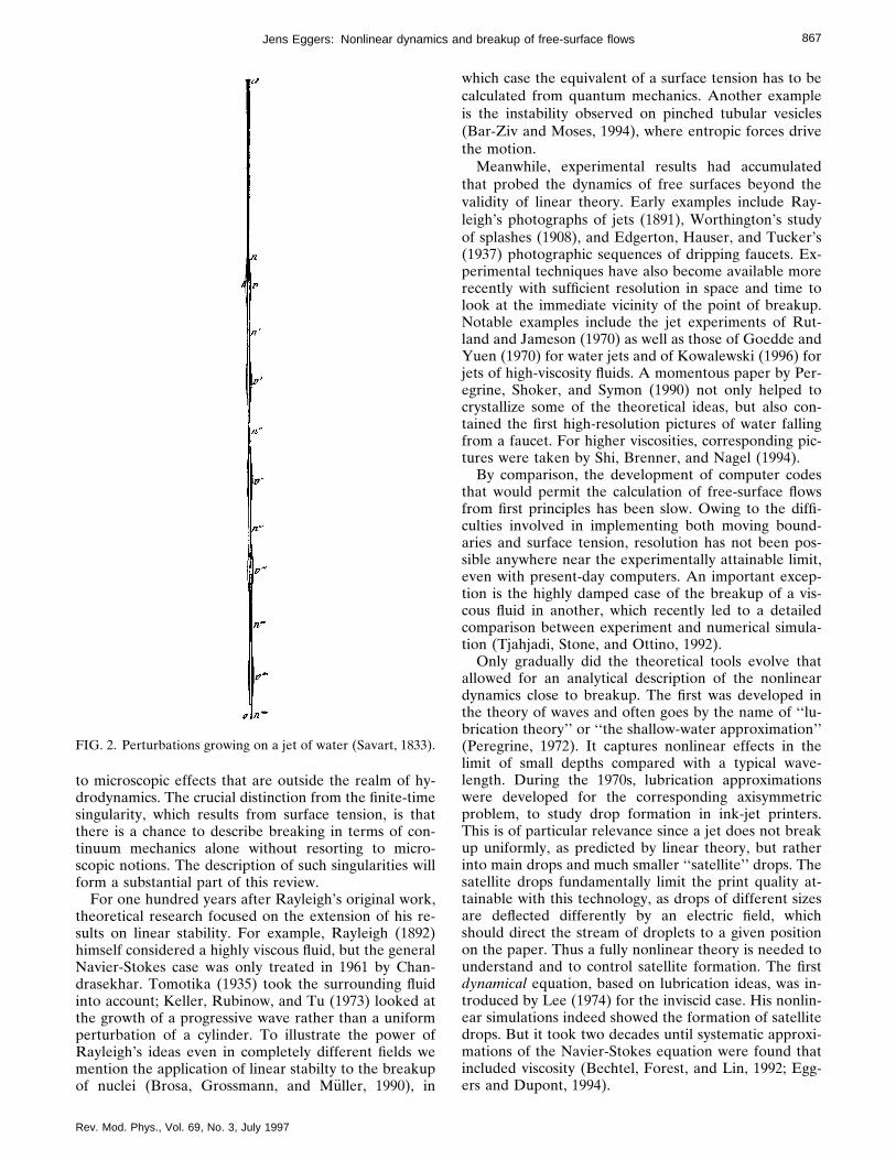
The basis for a more thorough understanding of dropformation was laid by Savart (1833), who very carefullyinvestigated the decay of fluid jets. By illuminating thejet with sheets of light, he observed tiny undulationsgrowing on a jet of water, as shown in Fig. 2. These
865(3)/865(65)/$19.75 © 1997 The American Physical Society

866 Jens Eggers: Nonlinear dynamics and breakup of free-surface flows
FIG. 1. A dolphin in the New EnglandAquarium in Boston, Massachusetts; Edger-ton (1977). © The Harold E. Edgerton 1992Trust, courtesy of Palm Press, Inc.
undulations later grow large enough to break the jet.Savart’s research showed that (i) breakup always occursindependent of the direction of gravity, the type of fluid,or the jet velocity and radius, and thus must be an in-trinsic property of the fluid motion; (ii) the instability ofthe jet originates from tiny perturbations applied to thejet at the opening of the nozzle.
In spite of his fundamental insights, Savart did notrecognize surface tension, which had been discoveredsome years earlier (de Laplace, 1805; Young, 1805) asthe source of the instability. This discovery was left to(Plateau 1849), who showed that perturbations of longwavelength reduce the surface area and are thus favoredby surface tension. On a level of quasistatic motion itwould thus be desirable to collect all the fluid into onesphere, corresponding to the smallest surface area. Evi-dently, as shown in Fig. 1, this does not happen. It wasRayleigh (1879a,1879b) who noticed that surface tensionhas to work against inertia, which opposes fluid motionover long distances. By considering small sinusoidal per-turbations on a fluid cylinder of radius r , Rayleigh foundthat there is an optimal wavelength, lR'9r , at whichperturbations grow fastest, and which sets the typicalsize of drops. Analyzing data Savart had obtained al-most 50 years earlier, Rayleigh was able to confirm histheory to within 3%.
Rev. Mod. Phys., Vol. 69, No. 3, July 1997
Accordingly, the time scale t0 on which perturbationsgrow and eventually break the jet is given by a balanceof surface tension and inertia, and thus
t05S r3r
g D 1/2
, (1)
where r is the density and g the coefficient of surfacetension of the fluid. This tells us two important things:Substituting the values for the physical properties of wa-ter and r51 mm, one finds that t0 is 4 ms, meaning thatthe last stages of pinching happen very fast, far belowthe time resolution of the eye. Secondly, as pinchingprogresses and r gets smaller, the time scale becomesshorter and pinching precipitates to form a drop in finitetime. At the pinch point, the radius of curvature goes tozero, and the small amount of fluid left in the pinchregion is driven by increasingly strong forces. Thus thevelocity goes to infinity, and the separation of a dropcorresponds to a singularity of the equations of motion,in which the velocity and gradients of the local radiusdiverge.
Even in the case of an infinite-time singularity of theequations of hydrodynamics, the physical event ofbreaking may occur in finite time. That is, when the fluidthread has become sufficiently thin, it may break owing
867Jens Eggers: Nonlinear dynamics and breakup of free-surface flows
to microscopic effects that are outside the realm of hy-drodynamics. The crucial distinction from the finite-timesingularity, which results from surface tension, is thatthere is a chance to describe breaking in terms of con-tinuum mechanics alone without resorting to micro-scopic notions. The description of such singularities willform a substantial part of this review.
For one hundred years after Rayleigh’s original work,theoretical research focused on the extension of his re-sults on linear stability. For example, Rayleigh (1892)himself considered a highly viscous fluid, but the generalNavier-Stokes case was only treated in 1961 by Chan-drasekhar. Tomotika (1935) took the surrounding fluidinto account; Keller, Rubinow, and Tu (1973) looked atthe growth of a progressive wave rather than a uniformperturbation of a cylinder. To illustrate the power ofRayleigh’s ideas even in completely different fields wemention the application of linear stabilty to the breakupof nuclei (Brosa, Grossmann, and Muller, 1990), in
FIG. 2. Perturbations growing on a jet of water (Savart, 1833).
Rev. Mod. Phys., Vol. 69, No. 3, July 1997
which case the equivalent of a surface tension has to becalculated from quantum mechanics. Another exampleis the instability observed on pinched tubular vesicles(Bar-Ziv and Moses, 1994), where entropic forces drivethe motion.
Meanwhile, experimental results had accumulatedthat probed the dynamics of free surfaces beyond thevalidity of linear theory. Early examples include Ray-leigh’s photographs of jets (1891), Worthington’s studyof splashes (1908), and Edgerton, Hauser, and Tucker’s(1937) photographic sequences of dripping faucets. Ex-perimental techniques have also become available morerecently with sufficient resolution in space and time tolook at the immediate vicinity of the point of breakup.Notable examples include the jet experiments of Rut-land and Jameson (1970) as well as those of Goedde andYuen (1970) for water jets and of Kowalewski (1996) forjets of high-viscosity fluids. A momentous paper by Per-egrine, Shoker, and Symon (1990) not only helped tocrystallize some of the theoretical ideas, but also con-tained the first high-resolution pictures of water fallingfrom a faucet. For higher viscosities, corresponding pic-tures were taken by Shi, Brenner, and Nagel (1994).
By comparison, the development of computer codesthat would permit the calculation of free-surface flowsfrom first principles has been slow. Owing to the diffi-culties involved in implementing both moving bound-aries and surface tension, resolution has not been pos-sible anywhere near the experimentally attainable limit,even with present-day computers. An important excep-tion is the highly damped case of the breakup of a vis-cous fluid in another, which recently led to a detailedcomparison between experiment and numerical simula-tion (Tjahjadi, Stone, and Ottino, 1992).
Only gradually did the theoretical tools evolve thatallowed for an analytical description of the nonlineardynamics close to breakup. The first was developed inthe theory of waves and often goes by the name of ‘‘lu-brication theory’’ or ‘‘the shallow-water approximation’’(Peregrine, 1972). It captures nonlinear effects in thelimit of small depths compared with a typical wave-length. During the 1970s, lubrication approximationswere developed for the corresponding axisymmetricproblem, to study drop formation in ink-jet printers.This is of particular relevance since a jet does not breakup uniformly, as predicted by linear theory, but ratherinto main drops and much smaller ‘‘satellite’’ drops. Thesatellite drops fundamentally limit the print quality at-tainable with this technology, as drops of different sizesare deflected differently by an electric field, whichshould direct the stream of droplets to a given positionon the paper. Thus a fully nonlinear theory is needed tounderstand and to control satellite formation. The firstdynamical equation, based on lubrication ideas, was in-troduced by Lee (1974) for the inviscid case. His nonlin-ear simulations indeed showed the formation of satellitedrops. But it took two decades until systematic approxi-mations of the Navier-Stokes equation were found thatincluded viscosity (Bechtel, Forest, and Lin, 1992; Egg-ers and Dupont, 1994).

868 Jens Eggers: Nonlinear dynamics and breakup of free-surface flows
Another important concept, which allows for the de-scription of nonlinear effects, is that of self-similarity(Barenblatt, 1996), which arises naturally in problemsthat lack a typical length scale. In the case of a singular-ity, the length scale of the solution will depend on time,reaching arbitrarily small values in the process. Thusself-similarity here means that the solution, observed atdifferent times, can be mapped onto itself by a rescalingof the axes. In the context of flows with surface tension,self-similarity was introduced by Keller and Miksis(1983). Kadanoff and his collaborators (Constantinet al., 1993; Bertozzi et al.., 1994) have looked at singu-larities in a Hele-Shaw cell, which is the two-dimensional analogue of the present problem, as asimple model for singularity formation. They inge-niously combined lubrication ideas and self-similarity toarrive at a detailed description of the pinchoff of abubble of fluid.
In the wake of this success, Eggers (1993) and Eggersand Dupont (1994) applied the same idea to the three-dimensional case. As spelled out first by Peregrine et al.(1990), the dynamics near breakup are independent ofthe particular setup such as jet decay, a dripping faucet,or even the complicated spraying shown in Fig. 1, butrather are characteristic of the nonlinear properties ofthe equations of motion. As the motion near a point ofbreakup gets faster, only fluid very close to that point isable to follow, making the breakup localized both inspace and time. Thus one expects the motion to becomeindependent of initial conditions, and the type of experi-ment becomes irrelevant to the study of the singular mo-tion. This brings about two crucial simplifications: (i) ina local description around the point of breakup, the mo-tion becomes ‘‘universal,’’ thus reducing the number ofrelevant parameters. The only parameter upon whichthe motion near the singularity still depends is the length
l n5n2r
g, (2)
which characterizes the internal properties of the fluid(Peregrine et al., 1990; Eggers and Dupont, 1994); (ii) anasymptotic analysis of the equations of motion revealsthat the motion close to the singularity is self-similar,with the radius shrinking at a faster rate than the longi-tudinal extension of the singularity. Near the pinchpoint, almost cylindrical necks develop, making the mo-tion effectively one-dimensional close to the singularity.
Using these ideas, a local solution of the Navier-Stokes equation was found, which contained no free pa-rameters (Eggers, 1993). To select a specific predictionof this theory, the minimum radius of a fluid thread at agiven time Dt away from breakup found to be
hmin50.03g
rnDt . (3)
The surface profiles calculated from theory have beencompared quantitatively and confirmed by experiment(Kowalewski, 1996). The columnar structure of the fluidneck allows for a stability analysis of the flow close tothe breaking point, and is modeled closely on Rayleigh’s
Rev. Mod. Phys., Vol. 69, No. 3, July 1997
analysis of a liquid cylinder (Brenner, Shi, and Nagel,1994; see also Brenner, Lister, and Stone, 1996). As theneck becomes sufficiently thin, it is prone to a finite-amplitude instability, which may be driven by thermalnoise. This causes secondary necks to grow on the pri-mary neck, which again have a self-similar form. Thecorresponding complicated structure of nested singulari-ties has also been observed experimentally (Shi, Bren-ner, and Nagel, 1994).
At the same time stability analysis indicates that cy-lindrical symmetry is not just a matter of convenience,but rather a generic property near breakup. Rayleigh’sanalysis tells us that any azimuthal variation results inonly a relative increase in surface area and is thus unfa-vorable. The universality and stability of the solutionnear breakup therefore lead to answers of a muchgreater generality than could be hoped for by investigat-ing individual geometries and initial conditions. At thesame time, the singular motion is the natural startingpoint for the calculation of nonlinear properties awayfrom breakup, which controls phenomena such as satel-lite formation. Another advantage of universality is thatonly one particular initial condition needs to be investi-gated to construct a unique continuation of the Navier-Stokes equation to times after the singularity (Eggers,1995a). This establishes that breaking is described bycontinuum mechanics alone, without resorting to a mi-croscopic description, as long as observations are re-stricted to macroscopic scales.
The scope of this review is limited mostly to the dy-namics in the immediate vicinity of the point of breakup.This is motivated by the expectation that pinching is uni-versal under quite general circumstances, even if themotion farther away from the singularity is more com-plicated. In the nonasymptotic regime, our focus is onthe axisymmetric case of a jet with or without gravity.This excludes many important examples of nonlinearfree-surface motion, such as drop oscillations, the dy-namics of fluid sheets, and in particular the vast field ofsurface waves.
We begin with an overview of the experimental basisof the subject. Here and in the rest of this review, weconfine ourselves to cylindrical symmetry. In the case offree surfaces, this is representative of the majority ofexperimental work in the physics literature. But it ex-cludes important effects like bending (Entov and Yarin,1984; Yarin, 1993), branching (Lin and Webb, 1994), andspraying (Yang, 1992) of jets. There is also substantialwork on splashes, i.e., the impact of drops on liquid(Og uz and Prosperetti, 1990) or on solid surfaces (Yarinand Weiss, 1995) surfaces. Mixing processes can also notbe expected to respect cylindrical symmetry. The outlineof experimental work in the second section is comple-mented by a review of numerical work in the third sec-tion. As indicated above, numerical simulations of thefull hydrodynamic equations are only slowly catching upwith the resolution possible in experiments. On theother hand, important information on the velocity fieldis not available experimentally. This and the superiorvariability of simulations, for example, in the choice of

869Jens Eggers: Nonlinear dynamics and breakup of free-surface flows
fluid parameters and of initial conditions, is bound tomake simulations an important source of information.
In the fourth section we give a detailed account oflinear stability theory, which is the classical approach tothe problem, but which remains an area of research tothe present day. Some nonlinear effects can be includedin perturbation theory, but the expansion quickly breaksdown near pinching.
The groundwork for the description of nonlinear ef-fects is laid by the development of one-dimensionalmodels. We spell out two different approaches to theproblem and explain some of the properties of the re-sulting models in Sec. V. In Sec. VI we study in detailthe universal self-similar solution leading up to breakup.The solution can be continued uniquely to a new solu-tion valid after breakup, which now consists of twoparts. The nonlinear stability theory of the asymptoticsolution explains the complicated structure seen in thepresence of noise.
Section VII explores the dynamics away from theasymptotic regime, but where nonlinear effects are stilldominant. The area best understood is the case of highlyviscous jets, in which the pinching has not yet becomesufficiently fast for inertial effects to become important.In the opposite limit of very low viscosity, the smoothingeffect of viscosity is missing, and gradients of the flowfield become large at a finite time away from breakup.This makes the problem a hard one, and the understand-ing of this regime is only in its early stages. However,this subject is bound to remain an interesting and fre-quently studied topic for the years to come, since lowviscosity fluids like water are the most common. From atheoretical point of view, the understanding of the sin-gularities of the Euler equation is one of the major un-solved problems in hydrodynamics, and fluid pinchingserves as a particularly simple model system. To con-clude Sec. VII, we describe some research on satelliteformation and present a numerical simulation of the sta-tionary state of a decaying jet.
So far we have dealt only with free surfaces, with sur-face tension being the only driving force. We relieve thisrestriction in the final section, where we explore someexamples of related topics. First we look at two-fluidsystems, which are particularly important for the theoryof mixing and the hydrodynamics of emulsions. Anasymptotic theory for breakup in the presence of anouter fluid has not yet been developed. Electric or mag-netic fields represent another possible external drivingforce. They force the fluid into sharp tips, where thefields are strong, out of which tiny jets are ejected. Thisallows for the production of very fine sprays. In chemicalprocessing, macromolecules are often present in solu-tion. They result in non-Newtonian properties of thefluid, to which we give a brief introduction in the contextof free-surface flows.
II. EXPERIMENTS
Historically, research on drop formation was moti-vated mostly by engineering applications, hence the
Rev. Mod. Phys., Vol. 69, No. 3, July 1997
three most common experimental setups, which are de-scribed in more detail below: (1) Jets are produced whena fluid leaves a nozzle at high speeds; (2) slow drippingunder gravity has been used for the measurement of sur-face tension; and (3) liquid bridges are used to suspendfluid in the absence of gravity. For a review on dropformation in the context of engineering applications ofspraying, see Walzel (1988). Early work focused eitheron the early stages of drop formation, characterized bythe growth of linear disturbances, or on the size andnumber of the resulting drops. Either aspect of drop for-mation is relatively easy to observe, but is highly depen-dent on the experimental setup and on parameters likenozzle diameter or jet speed.
Only slowly, as experimental techniques becameavailable for observing the actual evolution of the flowduring drop formation, did common features emergefrom the seemingly disparate results of individual ex-periments. The last stages of the evolution are domi-nated by the properties of the pinch singularity, which isthe same for all cases. This idea was first enunciatedclearly by Peregrine et al. (1990). The appearance of themotion depends only on the scale of observation l obsrelative to the size of the internal length l n [see Eq. (2)]of the fluid. If l obs /l n is large, which is typical for flowsof low viscosity like water, the shapes near the pinchpoint are cones attached to a spherical shell. Afterbreakup, as the fluid neck recoils, capillary waves areexcited. If on the other hand l obs /l n is small, as forfluids of high viscosity like glycerol, long and skinnythreads are observed, which rapidly contract into tinydrops after breakup. At the highest viscosities, thethreads tend to break at random places. It is from thisuniversality that much of the physical interest of the sub-ject of drop formation derives, and we try to emphasizecommon features in discussing different kinds of experi-ments.
A. Jet
By far the most widely used experimental setup in thestudy of drop formation is that of a jet of fluid leaving anorifice at high speeds. The earliest jet experiments wereperformed with fluid being driven out of holes near thebottom of a container (Bidone, 1823). The focus of theearly research was on the shape of jets produced by ori-fices of different forms. It was Savart (1833) who dis-tinctly noticed the inevitability of a decay into drops andcarefully investigated the laws governing it. By deliber-ately disturbing the jet periodically at the nozzle, he pro-duced disturbances on the surface of the jet with thesame frequency. Many other 19th-century researchersrepeated these experiments, notably Hagen (1849),Magnus (1855), and Rayleigh (1879b,1882). Both Pla-teau (1873) and Rayleigh were able to perform somequantitative tests of their theories, but without photog-raphy it was impossible to record the shapes of jets indetail. Photographic methods were introduced by Ray-leigh (1891), but these observations were only qualita-tive in nature. The first quantitative experiments were
870 Jens Eggers: Nonlinear dynamics and breakup of free-surface flows
those of Haenlein (1931), Donelly and Glaberson(1966), and Goedde and Yuen (1970). Their main con-cern was to test the linear theories of Rayleigh (1879a,1892) and Chandrasekhar (1961) for different viscosities.Goedde and Yuen also recorded shapes characterizingthe nonlinear behavior near breakup. Experiments fo-cusing on the measurement of satellites were performedby Rutland and Jameson (1970), Chaudhary and Max-worthy (1980a,1980b), and Vasallo and Ashgriz (1991).Becker, Hiller, and Kowalewski (1991, 1994) studied thenonlinear oscillations of drops produced in the breakupprocess. Their experimental setup was used by Kow-alewski (1996) to record surface shapes near breakupwith a spatial and temporal resolution far superior toprevious work. We shall describe this experiment insome detail, since it demonstrates the degree of sophis-tication the experimental technique has acquired overthe last few decades.
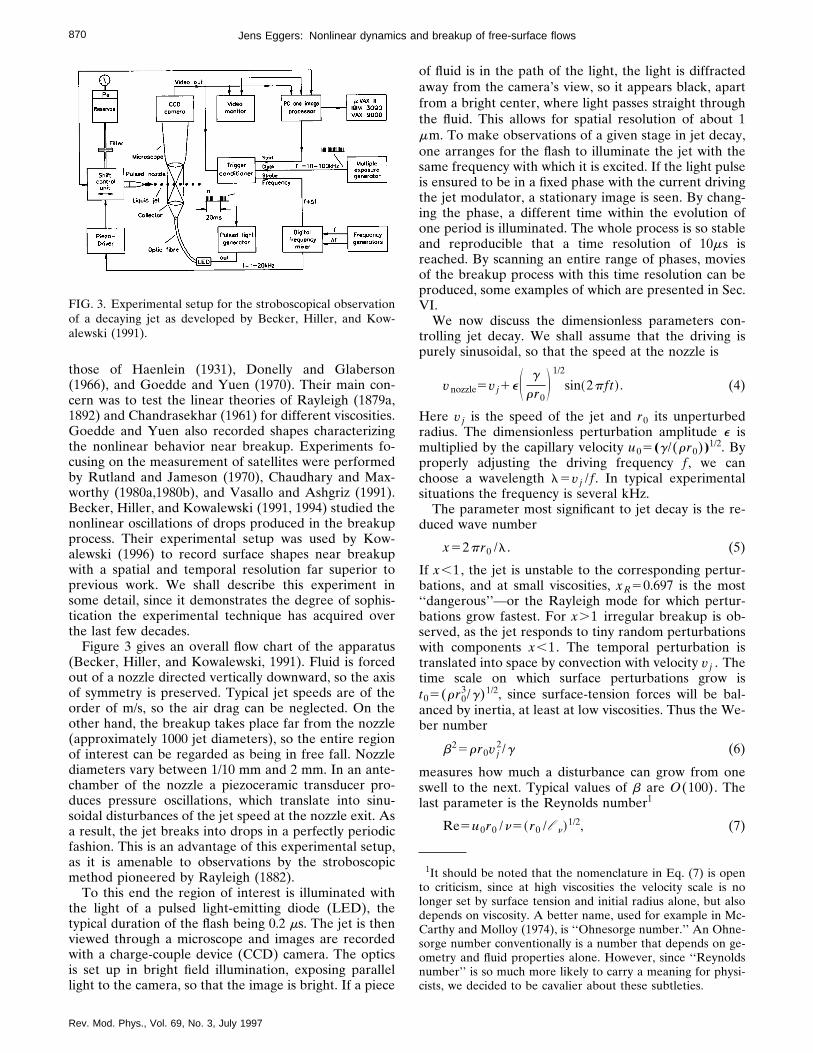
Figure 3 gives an overall flow chart of the apparatus(Becker, Hiller, and Kowalewski, 1991). Fluid is forcedout of a nozzle directed vertically downward, so the axisof symmetry is preserved. Typical jet speeds are of theorder of m/s, so the air drag can be neglected. On theother hand, the breakup takes place far from the nozzle(approximately 1000 jet diameters), so the entire regionof interest can be regarded as being in free fall. Nozzlediameters vary between 1/10 mm and 2 mm. In an ante-chamber of the nozzle a piezoceramic transducer pro-duces pressure oscillations, which translate into sinu-soidal disturbances of the jet speed at the nozzle exit. Asa result, the jet breaks into drops in a perfectly periodicfashion. This is an advantage of this experimental setup,as it is amenable to observations by the stroboscopicmethod pioneered by Rayleigh (1882).
To this end the region of interest is illuminated withthe light of a pulsed light-emitting diode (LED), thetypical duration of the flash being 0.2 ms. The jet is thenviewed through a microscope and images are recordedwith a charge-couple device (CCD) camera. The opticsis set up in bright field illumination, exposing parallellight to the camera, so that the image is bright. If a piece
FIG. 3. Experimental setup for the stroboscopical observationof a decaying jet as developed by Becker, Hiller, and Kow-alewski (1991).
Rev. Mod. Phys., Vol. 69, No. 3, July 1997
of fluid is in the path of the light, the light is diffractedaway from the camera’s view, so it appears black, apartfrom a bright center, where light passes straight throughthe fluid. This allows for spatial resolution of about 1mm. To make observations of a given stage in jet decay,one arranges for the flash to illuminate the jet with thesame frequency with which it is excited. If the light pulseis ensured to be in a fixed phase with the current drivingthe jet modulator, a stationary image is seen. By chang-ing the phase, a different time within the evolution ofone period is illuminated. The whole process is so stableand reproducible that a time resolution of 10ms isreached. By scanning an entire range of phases, moviesof the breakup process with this time resolution can beproduced, some examples of which are presented in Sec.VI.
We now discuss the dimensionless parameters con-trolling jet decay. We shall assume that the driving ispurely sinusoidal, so that the speed at the nozzle is
vnozzle5v j1eS g
rr0D 1/2
sin~2pft !. (4)
Here v j is the speed of the jet and r0 its unperturbedradius. The dimensionless perturbation amplitude e ismultiplied by the capillary velocity u05(g/(rr0))1/2. Byproperly adjusting the driving frequency f , we canchoose a wavelength l5v j /f . In typical experimentalsituations the frequency is several kHz.
The parameter most significant to jet decay is the re-duced wave number
x52pr0 /l . (5)
If x,1, the jet is unstable to the corresponding pertur-bations, and at small viscosities, xR50.697 is the most‘‘dangerous’’—or the Rayleigh mode for which pertur-bations grow fastest. For x.1 irregular breakup is ob-served, as the jet responds to tiny random perturbationswith components x,1. The temporal perturbation istranslated into space by convection with velocity v j . Thetime scale on which surface perturbations grow ist05(rr0
3/g)1/2, since surface-tension forces will be bal-anced by inertia, at least at low viscosities. Thus the We-ber number
b25rr0v j2/g (6)
measures how much a disturbance can grow from oneswell to the next. Typical values of b are O(100). Thelast parameter is the Reynolds number1
Re5u0r0 /n5~r0 /l n!1/2, (7)
1It should be noted that the nomenclature in Eq. (7) is opento criticism, since at high viscosities the velocity scale is nolonger set by surface tension and initial radius alone, but alsodepends on viscosity. A better name, used for example in Mc-Carthy and Molloy (1974), is ‘‘Ohnesorge number.’’ An Ohne-sorge number conventionally is a number that depends on ge-ometry and fluid properties alone. However, since ‘‘Reynoldsnumber’’ is so much more likely to carry a meaning for physi-cists, we decided to be cavalier about these subtleties.

871Jens Eggers: Nonlinear dynamics and breakup of free-surface flows
FIG. 4. Photographs of a decaying jet (Rut-land and Jameson, 1971) for three differentfrequencies of excitation. The bottom picturecorresponds to x50.683, which is close to theRayleigh mode. At longer wavelengths sec-ondary swellings develop (middle picture,x50.25), which cause the jet to break up attwice the frequency of excitation. At the long-est wavelength (top picture, x50.075) mainand secondary swellings have become virtu-ally indistinguishable. Reprinted with permis-sion of Cambridge University Press.
constructed from the jet radius r0 and the capillary ve-locity u0, divided by the kinematic viscosity n5h/r . Itmeasures the damping effects of viscosity on the motioncaused by surface tension. For water and a jet diameterof 1 mm, Re'200, but technologically relevant fluidscover a wide range of different viscosities. For example,in the case of glycerol the Reynolds number is reducedto 0.5, and by mixing water and glycerol a wide range ofReynolds numbers can be explored.
So, in the case of purely sinusoidal driving, there arefour dimensionless parameters governing jet decay: thedriving amplitude e , the reduced wave number x , theWeber number b2, and the Reynolds number Re. Therange of possible dynamics in this large parameter spacehas never been fully explored, so we shall focus on thedependence on the two most important parameters, thereduced wave number and the Reynolds number.
Figure 4 shows typical pictures of a decaying jet ofwater for three different wavelengths. The bottom pic-ture is for the mode of maximum instability. It is easilyfound by tuning the frequency, since it makes thebreakup point move closest to the nozzle. This situationis the least sensitive to noise, since all other frequencieshave lower growth rates and therefore decay relative tothe Rayleigh mode. Up to one wavelength from thepoint where a drop first separates, the disturbances lookfairly sinusoidal. (There are significant higher-order cor-rections, though, which will be discussed in Sec. IV.) Butthe last neck pinches off almost simultaneously at bothends, causing significant deviations from linear, sinu-soidal growth. This final, localized pinching producescharacteristic forms, namely, a sharp conical tip attachedto a flat cap. In recoiling, the tip excites capillary waveson its surface, which give it the appearance of a string ofpearls. While the tip is still recoiling, it breaks on its rearside and starts recoiling on the other side as well. Thus asmall satellite drop is produced, which is a remnant ofthe neck. In general it will receive momentum from therecoiling process and therefore has a velocity slightlydifferent from the main drops. This will make it mergeeither with the preceding or the following drop a fewwavelengths downstream.
Rev. Mod. Phys., Vol. 69, No. 3, July 1997
If the wavelength is long enough, the growth rate ofthe second harmonic will be larger than that of the pri-mary disturbance. Since higher harmonics are always ex-cited at the nozzle or through the nonlinear interaction,a swell develops in the middle between the drops. If ithas a chance to grow sufficiently large, the jet will breakin this l/2 mode and produce drops and satellites attwice the fundamental frequency of excitation. This isshown in the middle picture of Fig. 4 for a driving fre-quency that is a factor of 0.36 below the frequency cor-responding to the Rayleigh mode. The appearance ofsuch a ‘‘double stream’’ of droplets thus depends sensi-tively on the amplitude of the second harmonic pro-duced by the driving. Plateau (1857) used a cello to ex-cite the jet, and always found a double stream at half thefrequency of the Rayleigh mode. Later Rayleigh (1882)showed that this was due to harmonics inconvenientlyproduced by a musical instrument. Using tuning forksinstead, he still observed breakup with the principal fre-quency at a third of the Rayleigh frequency. For evenlonger wavelengths (top picture), the satellite drop be-comes substantial, owing to the much longer neck. Thiscauses the recoil patterns to be even more pronounced,since there is more time for capillary waves to develop.As a result, the satellite drop is subject to very compli-cated secondary breakings.
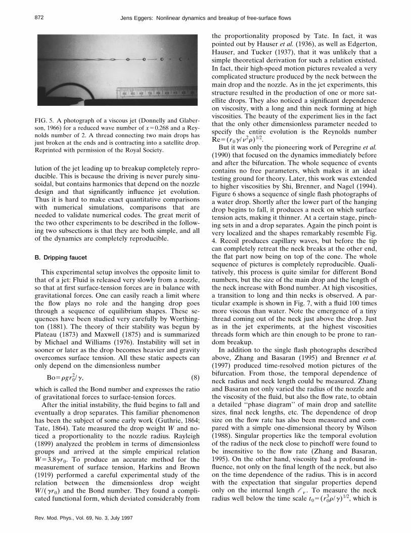
Decreasing the Reynolds number significantly, for ex-ample, by increasing the viscosity using a glycerol-watermixture, causes the breakup process to change substan-tially. After the initial sinusoidal growth, a region devel-ops where almost spherical drops are connected by thinthreads of almost constant thickness, which take quite along time to break (see Fig. 5). In general, the threadwill still break close to the swells. If the viscosity is in-creased further, the threads become so tenuous beforethey break at the end, that they break at several placesin between, in what seems to be a random breakup pro-cess.
Jet experiments are particularly useful for studyingthe universal motion near breakup with extremely highprecision, as we shall see in Sec. VI. On the other hand,it is hard to design an experiment to make the full evo-
872 Jens Eggers: Nonlinear dynamics and breakup of free-surface flows
lution of the jet leading up to breakup completely repro-ducible. This is because the driving is never purely sinu-soidal, but contains harmonics that depend on the nozzledesign and that significantly influence jet evolution.Thus it is hard to make exact quantitative comparisonswith numerical simulations, comparisons that areneeded to validate numerical codes. The great merit ofthe two other experiments to be described in the follow-ing two subsections is that they are both simple, and allof the dynamics are completely reproducible.
B. Dripping faucet
This experimental setup involves the opposite limit tothat of a jet: Fluid is released very slowly from a nozzle,so that at first surface-tension forces are in balance withgravitational forces. One can easily reach a limit wherethe flow plays no role and the hanging drop goesthrough a sequence of equilibrium shapes. These se-quences have been studied very carefully by Worthing-ton (1881). The theory of their stability was begun byPlateau (1873) and Maxwell (1875) and is summarizedby Michael and Williams (1976). Instability will set insooner or later as the drop becomes heavier and gravityovercomes surface tension. All these static aspects canonly depend on the dimensionless number
Bo5rgr02/g , (8)
which is called the Bond number and expresses the ratioof gravitational forces to surface-tension forces.
After the initial instability, the fluid begins to fall andeventually a drop separates. This familiar phenomenonhas been the subject of some early work (Guthrie, 1864;Tate, 1864). Tate measured the drop weight W and no-ticed a proportionality to the nozzle radius. Rayleigh(1899) analyzed the problem in terms of dimensionlessgroups and arrived at the simple empirical relationW53.8gr0. To produce an accurate method for themeasurement of surface tension, Harkins and Brown(1919) performed a careful experimental study of therelation between the dimensionless drop weightW/(gr0) and the Bond number. They found a compli-cated functional form, which deviated considerably from
FIG. 5. A photograph of a viscous jet (Donnelly and Glaber-son, 1966) for a reduced wave number of x50.268 and a Rey-nolds number of 2. A thread connecting two main drops hasjust broken at the ends and is contracting into a satellite drop.Reprinted with permission of the Royal Society.
Rev. Mod. Phys., Vol. 69, No. 3, July 1997
the proportionality proposed by Tate. In fact, it waspointed out by Hauser et al. (1936), as well as Edgerton,Hauser, and Tucker (1937), that it was unlikely that asimple theoretical derivation for such a relation existed.In fact, their high-speed motion pictures revealed a verycomplicated structure produced by the neck between themain drop and the nozzle. As in the jet experiments, thisstructure resulted in the production of one or more sat-ellite drops. They also noticed a significant dependenceon viscosity, with a long and thin neck forming at highviscosities. The beauty of the experiment lies in the factthat the only other dimensionless parameter needed tospecify the entire evolution is the Reynolds numberRe5(r0g/n2r)1/2.
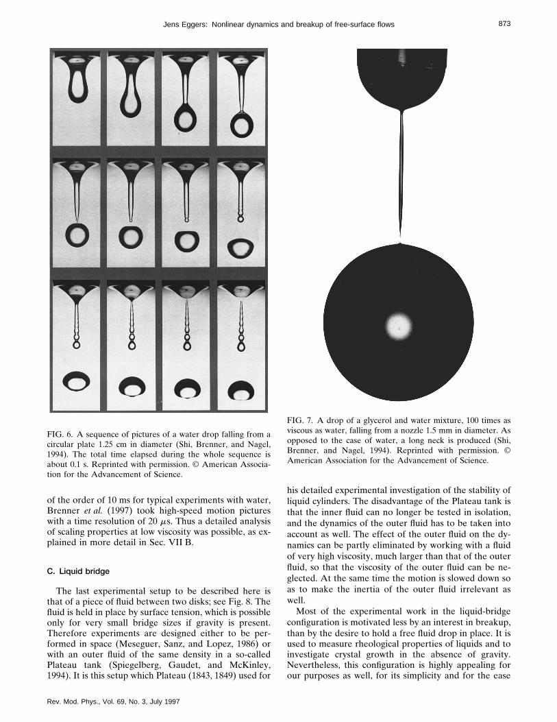
But it was only the pioneering work of Peregrine et al.(1990) that focused on the dynamics immediately beforeand after the bifurcation. The whole sequence of eventscontains no free parameters, which makes it an idealtesting ground for theory. Later, this work was extendedto higher viscosities by Shi, Brenner, and Nagel (1994).Figure 6 shows a sequence of single flash photographs ofa water drop. Shortly after the lower part of the hangingdrop begins to fall, it produces a neck on which surfacetension acts, making it thinner. At a certain stage, pinch-ing sets in and a drop separates. Again the pinch point isvery localized and the shapes remarkably resemble Fig.4. Recoil produces capillary waves, but before the tipcan completely retreat the neck breaks at the other end,the flat part now being on top of the cone. The wholesequence of pictures is completely reproducible. Quali-tatively, this process is quite similar for different Bondnumbers, but the size of the main drop and the length ofthe neck increase with Bond number. At high viscosities,a transition to long and thin necks is observed. A par-ticular example is shown in Fig. 7, with a fluid 100 timesmore viscous than water. Note the emergence of a tinythread coming out of the neck just above the drop. Justas in the jet experiments, at the highest viscositiesthreads form which are thin enough to be prone to ran-dom breakup.
In addition to the single flash photographs describedabove, Zhang and Basaran (1995) and Brenner et al.(1997) produced time-resolved motion pictures of thebifurcation. From those, the temporal dependence ofneck radius and neck length could be measured. Zhangand Basaran not only varied the radius of the nozzle andthe viscosity of the fluid, but also the flow rate, to obtaina detailed ‘‘phase diagram’’ of main drop and satellitesizes, final neck lengths, etc. The dependence of dropsize on the flow rate has also been measured and com-pared with a simple one-dimensional theory by Wilson(1988). Singular properties like the temporal evolutionof the radius of the neck close to pinchoff were found tobe insensitive to the flow rate (Zhang and Basaran,1995). On the other hand, viscosity had a profound in-fluence, not only on the final length of the neck, but alsoon the time dependence of the radius. This is in accordwith the expectation that singular properties dependonly on the internal length l n . To measure the neckradius well below the time scale t05(r0
3r/g)1/2, which is
873Jens Eggers: Nonlinear dynamics and breakup of free-surface flows
of the order of 10 ms for typical experiments with water,Brenner et al. (1997) took high-speed motion pictureswith a time resolution of 20 ms. Thus a detailed analysisof scaling properties at low viscosity was possible, as ex-plained in more detail in Sec. VII B.
C. Liquid bridge
The last experimental setup to be described here isthat of a piece of fluid between two disks; see Fig. 8. Thefluid is held in place by surface tension, which is possibleonly for very small bridge sizes if gravity is present.Therefore experiments are designed either to be per-formed in space (Meseguer, Sanz, and Lopez, 1986) orwith an outer fluid of the same density in a so-calledPlateau tank (Spiegelberg, Gaudet, and McKinley,1994). It is this setup which Plateau (1843, 1849) used for
FIG. 6. A sequence of pictures of a water drop falling from acircular plate 1.25 cm in diameter (Shi, Brenner, and Nagel,1994). The total time elapsed during the whole sequence isabout 0.1 s. Reprinted with permission. © American Associa-tion for the Advancement of Science.
Rev. Mod. Phys., Vol. 69, No. 3, July 1997
his detailed experimental investigation of the stability ofliquid cylinders. The disadvantage of the Plateau tank isthat the inner fluid can no longer be tested in isolation,and the dynamics of the outer fluid has to be taken intoaccount as well. The effect of the outer fluid on the dy-namics can be partly eliminated by working with a fluidof very high viscosity, much larger than that of the outerfluid, so that the viscosity of the outer fluid can be ne-glected. At the same time the motion is slowed down soas to make the inertia of the outer fluid irrelevant aswell.
Most of the experimental work in the liquid-bridgeconfiguration is motivated less by an interest in breakup,than by the desire to hold a free fluid drop in place. It isused to measure rheological properties of liquids and toinvestigate crystal growth in the absence of gravity.Nevertheless, this configuration is highly appealing forour purposes as well, for its simplicity and for the ease
FIG. 7. A drop of a glycerol and water mixture, 100 times asviscous as water, falling from a nozzle 1.5 mm in diameter. Asopposed to the case of water, a long neck is produced (Shi,Brenner, and Nagel, 1994). Reprinted with permission. ©American Association for the Advancement of Science.

874 Jens Eggers: Nonlinear dynamics and breakup of free-surface flows
FIG. 8. Liquid-bridge evolution starting froman unstable configuration. The disk diameteris 3.8 cm, the Reynolds number is 3.731023.The outer fluid, which eliminates buoyancyforces, has a viscosity approximately 1000times smaller than the inner fluid. (Spiegel-berg, Gaudet, and McKinley, 1994).
with which the experimental parameters can becontrolled. To begin with, the problem of static stabilityof the bridge becomes purely geometrical: it dependsonly on the radii of the disks and the volume of the fluid.This stability has been investigated theoretically in anumber of circumstances (Gillette and Dyson, 1971; Da-Riva, 1981).
If one wants to observe breaking, the bridge has to bemade unstable. This can be achieved either by suckingfluid from the bridge (Meseguer and Sanz, 1985) or bypulling the disks apart (Spiegelberg, Gaudet, and McK-inley, 1994). The latter method is illustrated in Fig. 8.The initial state was that of a cylinder with aspect ratioL5r0 /L50.77, where 2L is the distance between thedisks. Over a period of a few minutes, it was pulled apartto an aspect ratio of L51.58, which is an unstable con-figuration. The figure shows the collapse after the disksstopped moving. As expected for the extremely lowReynolds number of 3.731023, a thin thread forms be-fore the bridge finally breaks.
III. SIMULATIONS
In many areas of fluid mechanics, flow simulationshave become standard procedure. If the Reynolds num-ber is not too high, carefully executed simulations canvirtually replace experiments, since the validity of theequations of motion is not a source of concern. In thepresence of a free surface, however, the situation is dif-
Rev. Mod. Phys., Vol. 69, No. 3, July 1997
ferent. The flow geometry is essentially determined bythe evolution itself or may change its topology alto-gether due to breakup events. Thus computations needto be tailored to each initial condition. If breakup oc-curs, the validity of continuum mechanics, underlyingthe equations of motion, is itself called into question.This concern must be addressed separately through amore careful study of the singularities involved, orthrough complementing simulations of the underlyingmolecular dynamics (Greenspan, 1993; Koplik and Ba-navar, 1993).
Free-surface flows are also very sensitive to the for-mation of cusp singularities (Joseph et al., 1991) even inseemingly innocuous flow situations. It seems as if sur-face tension should make the surface more regular, thussimplifying simulations. But instead it offers very littleresistance to the formation of singularities (Jeong andMoffatt, 1992) and makes the system more sensitive tonoise and prone to numerical instabilities, whose nonlin-ear origins are poorly understood. Indeed, surface ten-sion introduces a complicated coupling between the flowthat advances the interface and the interface’s shape,which through the Young-Laplace equation determinesthe pressure driving the fluid.
For that reason, so-called boundary integral formula-tions are very attractive, since they involve only infor-mation about the surface of the fluid. They are possiblewhenever the flow is governed by a linear equation, forwhich the Green’s function is known. This is the case for
875Jens Eggers: Nonlinear dynamics and breakup of free-surface flows
inviscid, irrotational flow and highly viscous flow gov-erned by the Stokes equation. Then the only informa-tion needed apart from the position of the interface is itsvelocity. Thus one is relieved from calculating the subtleinterplay of internal motion and the boundary shape,since all the information is contained on the boundary.In the more general case of Navier-Stokes flow, the in-terior and the boundary have to be dealt with sepa-rately. Both the surface tracking and the flow computa-tions are highly nontrivial problems in themselves andare now coupled in a complicated fashion. Such compu-tations have been performed only fairly recently and arenot sufficiently accurate to resolve the universal behav-ior close to the singularity. Boundary integral methodsare more accurate, but neglect either viscous or inertialforces, both of which become important asymptotically.Nevertheless, simulations are an indispensable tool forpredicting the nonuniversal dynamics away frombreakup. One hopes that numerical codes will soon be-come sufficiently reliable to yield an alternative to ex-periments. A useful overview on computational methodsof free-surface flows is provided by Tsai and Yue (1996),who draw most of their examples from problems relatedto free-surface waves.
A. Inviscid, irrotational flow
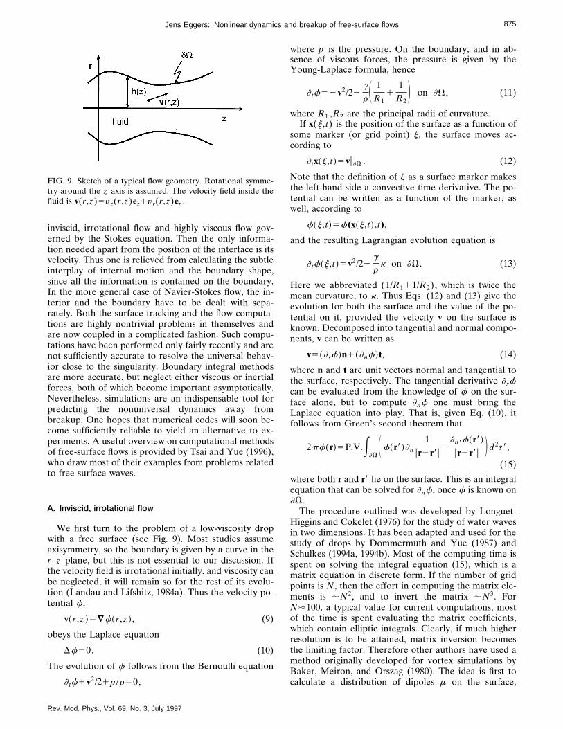
We first turn to the problem of a low-viscosity dropwith a free surface (see Fig. 9). Most studies assumeaxisymmetry, so the boundary is given by a curve in ther–z plane, but this is not essential to our discussion. Ifthe velocity field is irrotational initially, and viscosity canbe neglected, it will remain so for the rest of its evolu-tion (Landau and Lifshitz, 1984a). Thus the velocity po-tential f ,
v~r ,z !5“f~r ,z !, (9)
obeys the Laplace equation
Df50. (10)
The evolution of f follows from the Bernoulli equation
] tf1v2/21p/r50,
FIG. 9. Sketch of a typical flow geometry. Rotational symme-try around the z axis is assumed. The velocity field inside thefluid is v(r ,z)5vz(r ,z)ez1vr(r ,z)er .
Rev. Mod. Phys., Vol. 69, No. 3, July 1997
where p is the pressure. On the boundary, and in ab-sence of viscous forces, the pressure is given by theYoung-Laplace formula, hence
] tf52v2/22g
r S 1R1
11
R2D on ]V , (11)
where R1 ,R2 are the principal radii of curvature.If x(j ,t) is the position of the surface as a function of
some marker (or grid point) j , the surface moves ac-cording to
] tx~j ,t !5vu]V . (12)
Note that the definition of j as a surface marker makesthe left-hand side a convective time derivative. The po-tential can be written as a function of the marker, aswell, according to
f~j ,t !5f(x~j ,t !,t),
and the resulting Lagrangian evolution equation is
] tf~j ,t !5v2/22g
rk on ]V . (13)
Here we abbreviated (1/R111/R2), which is twice themean curvature, to k . Thus Eqs. (12) and (13) give theevolution for both the surface and the value of the po-tential on it, provided the velocity v on the surface isknown. Decomposed into tangential and normal compo-nents, v can be written as
v5~]sf!n1~]nf!t, (14)
where n and t are unit vectors normal and tangential tothe surface, respectively. The tangential derivative ]sfcan be evaluated from the knowledge of f on the sur-face alone, but to compute ]nf one must bring theLaplace equation into play. That is, given Eq. (10), itfollows from Green’s second theorem that
2pf~r!5P.V.E]V
S f~r8!]n
1ur2r8u
2]n8f~r8!
ur2r8u Dd2s8,
(15)
where both r and r8 lie on the surface. This is an integralequation that can be solved for ]nf , once f is known on]V .
The procedure outlined was developed by Longuet-Higgins and Cokelet (1976) for the study of water wavesin two dimensions. It has been adapted and used for thestudy of drops by Dommermuth and Yue (1987) andSchulkes (1994a, 1994b). Most of the computing time isspent on solving the integral equation (15), which is amatrix equation in discrete form. If the number of gridpoints is N , then the effort in computing the matrix ele-ments is ;N2, and to invert the matrix ;N3. ForN'100, a typical value for current computations, mostof the time is spent evaluating the matrix coefficients,which contain elliptic integrals. Clearly, if much higherresolution is to be attained, matrix inversion becomesthe limiting factor. Therefore other authors have used amethod originally developed for vortex simulations byBaker, Meiron, and Orszag (1980). The idea is first tocalculate a distribution of dipoles m on the surface,

876 Jens Eggers: Nonlinear dynamics and breakup of free-surface flows
which produce the potential f . This can be done effi-ciently by iteration. The dipole distribution is then usedto calculate the normal component of the velocity field,which is an N2 process. For the present problem, thisprocedure has been adopted by Og uz and Prosperetti(1990) and Mansour and Lundgren (1990).
To formulate the system comprised by Eqs. (12)–(15)in discrete numerical form, a number of different proce-dures were adopted, some of which are compared byPelekasis, Tsamopoulos, and Manolis (1992). Usuallythe position of the interface x and the potential f istaken at a discrete set of nodes i , 1<i<N . Using suit-able interpolation formulas, one evaluates the curvatureat the interface and the integral in Eq. (15). An explicitRunge-Kutta step is then used to advance the position ofthe interface xi and the potential f i . However, a prob-lem that appears, regardless of the numerical implemen-tation, is nonlinear instability on the scale of the gridspacing, giving the interface a saw-tooth appearance.The origin of this instability has not yet been found.Moore (1983), investigating a model problem, has shownthat such short-wavelength instabilities may be a resultof spatial discretization. But since the instability was re-ported in all work on the problem, using many differentnumerical techniques, there is a distinct possibility thatthe evolution equations (10), (12), and (13) do not pos-sess regular solutions, but rather have unphysical singu-larities before breakup occurs. One has to bear in mindthat the underlying equations are inviscid, so there is nonatural way for momentum to be diffused, and cata-strophically sharp gradients can occur, just as in thethree-dimensional Euler equation with large-scale driv-ing (Majda, 1991). This analogy is of course a very roughone, since singularities in the three-dimensional Eulerequation come about through the growth of vorticity,which is constrained to be zero in the present case ofirrotational flow.
A number of different procedures have been pro-posed to get rid of the instability. Grid points were re-distributed after every time step to ensure equal gridspacing (Dommermuth and Yue, 1987; Og uz and Pros-peretti, 1990; Schulkes, 1994a). This step removes short-wavelength components and results in some numericalenergy dissipation (Schulkes, 1994a). Other possibilitiesare the inclusion of numerical diffusion (Og uz and Pros-peretti, 1990; Pelekasis, Tsamopoulos, and Manolis,1992), or simply filtering of the short-wavelength com-ponents (Dold, 1992).
Only a few papers have focused on drop formation,namely those of Mansour and Lundgren (1990), whosimulated a liquid cylinder with periodic boundary con-ditions; Spangler, Hilbing, and Heister (1995), who in-cluded the effect of a surrounding gas; and Schulkes(1994b), who considered a dripping faucet. The spatiallyuniform liquid cylinder is only a rough approximation ofthe steady state of a decaying liquid jet, but the simula-tions qualitatively produce the correct features. In par-ticular, Mansour and Lundgren predict satellite drops atall wave numbers, whose volumes agree well with ex-periment.
Rev. Mod. Phys., Vol. 69, No. 3, July 1997
Schulkes (1994b) directly compares his simulationwith the experiment by Peregrine et al. (1990) and findsgood agreement, except in the immediate neighborhoodof the bifurcation point (see Fig. 10). Instead of formingan almost flat interface at the side of the drop, the pro-file turns over in the inviscid simulation. This seems tobe a universal feature of this approximation, as a similaroverturning is observed for the initial condition consid-ered by Mansour and Lundgren. In experiments, a verylarge, but still finite, slope is observed. The steepening ofthe interface has been the subject of a recent experimen-tal and numerical study (Brenner et al., 1997).
Overturning thus seems to be an artifact of the invis-cid theory, since the viscosity does become important asthe interface becomes steeper, as will be discussed inmore detail in Sec. VII.B. The inviscid approximation isthus invalidated even on scales much larger than l n .However, overturning is observed after breaking, whenthe small remnant of the neck on the drop side recoils.The momentum it acquires is large enough to produce adent on the flat surface of the drop. In experimentalpictures, which usually show a projection perpendicularto the axis of symmetry, it turns up as a perfectly straightinterface, as seen in the sixth frame of Fig. 6. It would beworthwhile to take pictures at an angle as well, to fur-ther investigate the dented region.
B. Stokes flow
The other case that can be treated by boundary inte-gral methods is that of a highly viscous fluid, describedby the Stokes equation
hDv5“p . (16)
FIG. 10. The shape of a drop of water falling from a nozzle atthe first bifurcation. The Bond number is Bo=1.02 and theReynolds number Re=452. The comparison with theory (solidline) is taken from Schulkes (1994b). Reprinted with permis-sion of Cambridge University Press.

877Jens Eggers: Nonlinear dynamics and breakup of free-surface flows
Here inertial terms have been dropped, so the fluid den-sity does not appear. For Eq. (16) Green’s functions areknown (Ladyzhenskaya, 1969), so that an integral equa-tion for the interfacial velocity can be derived in thesame vein as in the inviscid case. This was first accom-plished by Youngren and Acrivos (1975) for a gasbubble in a very viscous fluid. The method has beengeneralized by Rallison and Acrivos (1978) to the caseof drops of arbitrary viscosity in another viscous fluid.However, the early numerical work on viscous dropswas limited to the calculation of stationary shapes (Ral-lison, 1984).
Only some years later did Stone and Leal (1989a,1989b) develop codes of sufficient accuracy to study thedynamics of extended drops. Because of the ample vis-cous damping, this problem is much less sensitive to per-turbations, and no numerical instabilities have been re-ported. Most of the work concerns a drop of fluid inanother fluid, which is quiescent at infinity. However,the viscosity of the outer fluid can be taken to be zero,so the drop is isolated.
Some pictures of extended drops breaking up are con-tained in Stone and Leal (1989b). The shape of the in-terface near breakup and the velocity field is studied insome detail. But only Tjahjadi, Stone, and Ottino (1992)demonstrated the full power of viscous boundary inte-gral methods by performing a quantitative comparisonwith experiments on viscous drops in extensional flows.This study showed extraordinary agreement betweensimulation and experiment, which continued through anumber of breakups (see Fig. 11), and revealed an as-tonishingly fine structure of satellite drops. Breakup wassimulated by cutting the interface and smoothing theends once some critical radius was reached. As the fluidmoves faster and faster near breakup, the Stokes ap-proximation eventually will break down, but on thescales observed it seems to remain remarkably good. Asimilar Stokes code has recently been applied to astretching liquid bridge (Gaudet, McKinley, and Stone,1996). The results are in excellent agreement with ex-perimental data, and in addition supply a wealth of in-formation about the dynamics of the bridge at differentviscosity ratios and stretching rates.
C. Navier-Stokes simulations
The boundary integral methods described in the firstsubsection are valid only for very low or very high vis-cosity. As we we are going to see in Sec. VII, eitherapproximation breaks down close to the pinch point,where viscous or inertial effects become important, atleast in the case that the outer fluid can be neglected. Inthose cases, the full Navier-Stokes equation has to besolved in the fluid domain, subject to a singular forcingat the boundary. Even in a fixed domain this is not asimple problem, so it is not surprising that Navier-Stokessimulations in the nonlinear regime are few. Still, resultsfrom first-principles calculations are indispensable, asthey provide the full information on the flow field, whichis not available from experiment. Johnson, Marschall,
Rev. Mod. Phys., Vol. 69, No. 3, July 1997
and Esdorn (1985) and Marschall (1985) provide someexperimental measurements of the flow field, but the re-gion near the point of breakup is particularly hard tovisualize, so the flow field is not known here.
The interior of the flow is described by the Navier-Stokes equation
] tv1v~¹v!521r
“p1nDv (17)
for incompressible flow
¹v50. (18)
Here v(r,t) is the three-dimensional velocity field andp(r,t) the pressure. On the free boundary, pressure andviscous forces are balanced by capillary forces:
s•n52gknu]V . (19)
In this formula, s is the stress tensor and n the normalvector pointing out of the fluid. With the velocityknown, the interface is moved according to Eq. (12).
The main technical problem, as compared to otherNavier-Stokes simulations, involves the coupling to amovable interface and the treatment of a varying com-putational domain. The earliest work is that by Fromm(1984), who uses a square grid with a refined grid super-imposed on it to track the surface. The paper focuses on
FIG. 11. Time evolution of a highly extended fluid suspendedin another fluid. The viscosity ratio is 0.067, and the dimen-sionless wave number is 0.5. The times the snapshots weretaken are shown in the middle (Tjahjadi, Stone,and Ottino,1992). Reprinted with permission of Cambridge UniversityPress.

878 Jens Eggers: Nonlinear dynamics and breakup of free-surface flows
the specific problem of ink-jet technology and does notstudy pinching systematically. In the work by Shokoohiand Elrod (1987, 1990), the computational domain ismapped onto a cylinder with radius 1, making surfacetracking superfluous. The price one has to pay is that theequations in the interior get very complicated. In par-ticular, the earlier paper (Shokoohi and Elrod, 1987)contains a number of surface profiles for different initialdisturbances at a fixed Reynolds number of Re550.
The technique most appropriate for the problem isprobably the one adopted by Keunings (1986), whichuses a deformable grid to accommodate the moving in-terface. A similar technique was recently used in themost extensive study of breakup to date (Ashgriz andMashayek, 1995). Here the fluid is bounded by a heightfunction h(z ,t); see Fig. 9. Thus one is limited to situa-tions in which the profile does not overturn. The com-putational domain is divided into quadrangles in the r–z plane, four of which constitute a column in the radialdirection. On each of the quadrangles, four shape func-tions are defined, into which the flow field is expanded.Using a Galerkin method, one can derive a discrete setof equations for the amplitudes of the velocity field andthe boundary points hi . To follow the motion of theinterface, the mesh points are allowed to move in theradial direction. This is done in such away as to ensuremass conservation in each element. From this the freesurface is reconstructed. Simulations are reported over awide range of Reynolds numbers up to Re=200, whichcorresponds to a water jet of 1 mm in diameter. No nu-merical instabilities are reported even at the highestReynolds number.
Simulations were performed with periodic boundaryconditions in the axial direction and for initial sinusoidaldisturbances of different wave numbers. The resultswere tested against the predictions of linearized theory(Rayleigh, 1879a; Chandrasekhar, 1961), which are dis-cussed in greater detail in the next section. The overallagreement with predicted growth rates is good. The larg-est deviations occur for the highest Reynolds number,for which a maximum error of 10% is reported. Particu-larly interesting is a sequence of pictures testing the non-linear evolution leading to breakup for a variety of wavenumbers and Reynolds numbers. Although the wavenumber affects the overall shape, the appearance of theinterface near the point of breakup is very similar fordifferent wave numbers. However, viscosity affects thebreakup significantly: just as seen in experiment, the in-terface looks like a cone attached to a steep front forlow viscosities and gets increasingly flat for higher vis-cosities. We shall study the interfacial shape in greaterdetail when we compare it with the results of one-dimensional models (see Sec. V). One very importantpoint to notice right away is that overturning of the pro-file does not occur, even at the highest Reynolds num-bers, which are comparable with experimental ones withwater.
Almost all the work described so far deals with theproblem up to the point of first breakup. To continuethrough the singularity, some ad hoc prescription for a
Rev. Mod. Phys., Vol. 69, No. 3, July 1997
continuation has to be invented for each particular case,as was done in Tjahjadi, Stone, and Ottino (1992) orSchulkes (1994b). Apart from the theoretical questionsinvolved, it would be desirable to develop a general phe-nomenological scheme to describe breakup and mergingin an arbitrary geometry. Instead of tracking the inter-face with surface markers (‘‘front tracking’’), this is mosteasily accomplished by describing the interface by a sca-lar function C(r,t), which is defined everywhere (‘‘frontcapturing’’). This function is 0 in one fluid and 1 in theother. The crossover region represents the interface,which is maintained to have some finite thickness bynumerical diffusion. The function C is advanced every-where according to
] tC1v~“C !50. (20)
Obviously this description does not rely on specific as-sumptions about the connectivity of the fluid domains.On a ‘‘microscopic’’ scale set by numerical diffusion, athin sliver of fluid is dissolved and thus broken. Con-versely, if two pieces of fluid come sufficiently close,they are joined. The most widely used variant of thisidea is the ‘‘volume-of-fluid method’’ developed by Hirtand Nichols (1981), which is designed to conserve vol-ume exactly. Surface tension is included in two recentpapers by Lafaurie et al. (1994), and by Richards, Len-hoff, and Beris (1994) by distributing surface-tensionforces continuously across the interface. The formergroup emphasizes collision and merging of drops, thelatter studies breakup of jets. The computational do-main, on which the Navier-Stokes solver operates, is sta-tionary. Figure 12, showing two drops colliding at highspeeds and their subsequent breakup, nicely illustratesthe generality of this method.
On the other hand, the resolution available nearbreakup is not very high, so the singularity cannot bestudied in detail. Lafaurie et al. (1994) also report somenumerical instabilities at large Reynolds numbers. Sodespite some remarkable features, the development ofgeneral-purpose codes capable of faithfully resolvingbreakup in some detail remains a challenge for the fu-ture.
As a last possibility, we mention the work of Becker,Hiller, and Kowalewski (1994). It is concerned withlarge-amplitude droplet oscillations. The Navier-Stokesequation is here analyzed by expanding the velocity fieldinto a set of eigenmodes of the linear problem. Thismethod is very efficient when surface deformations arenot too large, so that they are representable by a reason-able number of eigenmodes. However, one expects it tobecome inefficient close to rupture, where typical flowfields are dissimilar to eigenmodes of the linear problem.
IV. SMALL PERTURBATIONS
A. Linear stability
For a piece of fluid to break up, it must be unstableagainst surface tension forces at some point during itsevolution. If the fluid is at rest initially, or the time scale

879Jens Eggers: Nonlinear dynamics and breakup of free-surface flows
FIG. 12. Frontal collision of two drops at We-ber number b2520 and Reynolds number Re=250, based on the relative velocity of thedrops (Gueyffier and Zaleski, 1997). First atoroidal structure is formed, which then col-lapses and forms a cylinder. This cylinderbreaks up as required by the Rayleigh insta-bility.
of the surface-tension-induced motion is much shorterthan other time scales, then the problem of stability ispurely geometrical; that is, instability means that thesurface area can be reduced by an infinitesimal surfacedeformation.
The classical example studied by Plateau (1873) andRayleigh (1896) is that of an infinitely long cylinder ofradius r0. To a good approximation such a fluid cylinderwill be produced by a jet emanating from a nozzle athigh speed. Now one considers a sinusoidal perturbationof wavelength l on the cylinder. For example, any ran-dom perturbation on the jet may be decomposed into alinear superposition of such Fourier modes. In a linearapproximation all the modes evolve independently, andone may consider just a single sinusoidal perturbation.In most practical applications, however, perturbations ofa given wavelength are produced at the nozzle and areconvected down the jet. As argued in Sec. II, for largeWeber numbers b25rr0v j
2/g this results in periodic dis-turbances, which are practically uniform in space.
In cylindrical coordinates r ,w ,z the surface shape canbe written as r(w ,z). It is convenient to measure theaxial coordinate z and deviations from the cylindricalshape r(w ,z)5r0 in units of r0:
z5z/r0 (21)
and
Rev. Mod. Phys., Vol. 69, No. 3, July 1997
r~w ,z !/r0511h~w ,z!. (22)
In addition to the sinusoidal perturbation of the radius,we also allow for small departures from the circularcross section. This is taken care of by an additional azi-muthal dependence of the initial perturbation:
h~w ,z!5e cos~nw!cos~xz!,
x5kr0 .
The dynamical constraint is that the volume
V/r035
12E0<z<2p/x
~11h!2dwdz
52p2
x H 11e2/2 n50
11e2/4 n51,2, . . .
per wavelength is kept constant as e evolves in time.This means h must also contain another contributionwhich ensures conservation of mass, and thus
h~w ,z!5e cos~nw!cos~xz!2e2~11dn0!/81O~e4!.(23)
On the other hand, the surface area is

)
880 Jens Eggers: Nonlinear dynamics and breakup of free-surface flows
A/r025E
0<z<2p/xF11~]zh!21S ]wh
11h D 2G1/2
3~11h!dwdz
5~2p!2
x H 11e2
8~11dn0!~x21n221 !J . (24)
Hence with growing disturbance amplitude e the surfacearea decreases only if disturbances are axisymmetric(n50) and x,1. In other words, the wavelength of aperturbation must be greater than p times the diameterof the jet for it to be unstable. This famous result is dueto Plateau (1849). From this it may seem as if distur-bances of very long wavelength, i.e., small x , are themost rapidly growing ones, as they reduce the surfacearea the most. But this leaves out the dynamics of theproblem, which we have not considered yet. In fact, sur-face tension has to overcome both inertia and viscousdissipation. The problem first treated by Rayleigh(1879a) is that of a low-viscosity fluid like water, forwhich inviscid theory applies.
Following Rayleigh, we shall calculate the optimal orfastest growing mode xR , 0,xR,1. If a jet is disturbedrandomly by external noise, this will usually be themode that sets the size of drops, as it will soon dominateall the other excited modes. We shall consider only axi-symmetric perturbations here, since all nonaxisymmetricperturbations only create more surface area and aretherefore stable. For most of this subsection, we shall belooking at inviscid irrotational flow, so the velocity fieldhas a potential f(r ,z ,t), and Eqs. (10), (12), and (13) foran ideal fluid apply.
The velocity potential is nondimensionalized using theinitial jet radius r0 and the time scale t05(rr0
3/g)1/2,which implies a balance of surface tension and inertialforces. Hence
f~r ,z ,t!5t0
r02 f~r ,z ,t !, (25)
where
r5r/r0 , z5z/r0 , and t5t/t0 . (26)
No confusion of the variable r with the density shouldarise here. The nondimensional equations of motion arethus
Df50,
]th5]rf2~]zf !~]zh!ur511h , (27)
]tf51212
@~]rf !21~]zf !2#
21
A11~]zh!2F 111h
2]z
2h
11~]zh!2GUr511h
.
The initial conditions are
h~z ,0!5e cos~xz!2e2/41O~e4!, (28)
]th~z ,0!50.
Rev. Mod. Phys., Vol. 69, No. 3, July 1997
Since the initial surface displacement is assumed to beproportional to some small parameter e , the velocity willalso be small, so we try the expansion
f~r ,z ,t!5ef1~r ,z ,t!1O~e2!, (29)
h~r ,z ,t!5eh1~r ,z ,t!1O~e2!.
To first order in e , the equations of motion (27) become
S ]r21
]r
r1]z
2Df150, (30a)
]th15]rf1ur51 , (30b)
]tf15h11]z2h1ur51 . (30c)
Looking for solutions of the form
h15A1~t!cos~xz!, (31)
f15B1~t!f~r!cos~xz!,
we find from Eq. (30a)
f91f8/r2x2f50.
The only solution that is regular for r50 isf(r)5I0(xr), where I0 is a modified Bessel function ofthe first kind. Substituting this into the boundary condi-tions (30b) and (30c) gives
]tA15B1xI1~x ! and ]tB1I0~x !5A1~12x2!.
The solution of this set of equations with the initial con-ditions (28), namely, A1(0)51, ]tA1(0)50, is
A1~t!5cosh~v t!, B1~t!5v
xI1~x !sinh~v t!, (32
with
v 25xI1~x !
I0~x !~12x2!. (33)
Frequencies are measured in units of the inverse timescale v05(g/(rr0
3))1/2. The dimensionless growth ratev 5v/v0 is real for x,1, so perturbations grow expo-nentially, making the jet unstable against arbitrarilysmall perturbations. For x.1, on the other hand, theinterface performs oscillations, which will eventually bedamped by viscosity. The inviscid dispersion relation(33) is plotted in Fig. 13. The most unstable mode, cor-responding to the largest v , occurs at xR50.697. This isthe famous Rayleigh mode, which has a wavelengthlR59.01r0.
This result can be checked directly against the obser-vations by Savart (1833). If a jet is excited at the nozzleof a reservoir, it will break with the same frequency withwhich it is excited. If the impact of the resulting dropson another container is fed back into the reservoirthrough a mechanical coupling, the original perturbationwill be amplified. This amplification is greatest for themost unstable wave numbers, and strong enough for amusical note to sound. Savart measured the pitch of thesound, and from this observation Plateau (1849) inferreda wavelength of 4.38 times the diameter of the jet. Usinghis concept of maximum instability, Rayleigh (1879b)

881Jens Eggers: Nonlinear dynamics and breakup of free-surface flows
was finally able to interpret this result and found it to beremarkably close to the prediction of his theory.
The first accurate measurement of the complete dis-persion relation was done by Donelly and Glaberson(1966). They excited a water jet with a loudspeaker andobserved photographically how perturbations grow fromone wave crest to the next. Knowing the jet velocity,they could obtain the temporal growth rate of the per-turbations. Instead of measuring the height of the crestswith respect to r0, it is more convenient to take the dif-ference between nodes and crests, which Donelly andGlaberson found to exhibit exponential growth up toone wavelength from the breakup point. This may bedue in part to a cancellation of nonlinear effects, asclaimed by Yuen (1968) and confirmed by Goedde andYuen (1970). That is, when one takes the difference be-tween crests and valleys, the contribution from second-order perturbation theory drops out. Both Donelly andGlaberson (1966) and Goedde and Yuen (1970) foundexcellent agreement with Rayleigh’s dispersion relationto within experimental scatter. The experimental pointshave been included in Fig. 13. It should be mentionedthat an earlier investigation (Crane, Birch, and McCor-mack, 1964) had found deviations from linear theorybased on both the breakup length and direct analysis ofphotographs. The authors attributed this to the large dis-turbance amplitude used in their experiment, makinglinear theory inapplicable.
It was first pointed out by Plateau (1873) that viscositymight considerably alter the above results. As onecomes closer and closer to a quasistatic Stokes descrip-tion, inertia becomes less and less important, and themost unstable wavelength becomes longer, correspond-ing to the greatest reduction in surface area. Rayleighhimself analyzed the case of very large viscosities (Ray-leigh, 1892), assuming that the fluid is described by theStokes equation. The full problem, using the Navier-Stokes equation, was first treated in the monograph byChandrasekhar (1961). The result for v is a complicatedimplicit equation, which offers little insight in itself, so it
FIG. 13. The dimensionless growth rate of sinusoidal pertur-bations on a cylinder as a function of the dimensionless wavenumber. The solid line represents Rayleigh’s theory for invis-cid flow, the squares are data from Donnelly and Glaberson(1966), triangles are from Goedde and Yuen (1970).
Rev. Mod. Phys., Vol. 69, No. 3, July 1997
is not reproduced here. Instead, we give the result thatcomes from expanding Chandrasekhar’s formula forsmall x5kr0. It is
v5v0H F12
x2~12x2!194
Re22x4G1/2
232
Re21x2J .
(34)
This equation was first obtained by Weber (1931), whoanalyzed the motion of thin slices of fluid. Surprisingly,it turns out to be a uniformly good approximation for allwavelengths and viscosities. For zero viscosity, it is offby 7% at most, and becomes increasingly accurate forhigher viscosities. According to Eq. (34), the fastest-growing mode is
xR2 5
1
21A18/Re, (35)
which gets smaller with growing viscosity.As the Reynolds number decreases, the growth rate is
eventually determined by a balance of surface tensionand viscous forces alone, rather than inertial forces. Thedispersion relation (34) gives, in the limit of small Rey-nolds number,
v5vn
16
~12x2!, (36)
where vn5g/(r0rn) is a viscous growth rate. The vis-cous dispersion relation has been tested by Donelly andGlaberson (1966) and Goedde and Yuen (1970), whoboth found good agreement with Chandrasekhar’s(1961) results. A typical dispersion relation is shown inFig. 14 for Re51.73.
Since Rayleigh’s pioneering work, linear stability ofliquid cylinders has been applied to many other physicalsituations. Tomotika (1935) generalized Rayleigh’s(1892) analysis of a highly viscous column to include anouter fluid of finite viscosity and density. Both fluids aredescribed by Stokes’ equation. It was found that themost unstable wavelength varied with the ratio of thetwo viscosities. A simple formula describing the case oftwo equal viscosities has been given by Stone and Bren-ner (1996). We shall come back to the problem ofbreakup of one fluid in another in Sec. VIII.A.
The influence of a surrounding gas of low density wasstudied by Weber (1931), Lin and Kang (1987), and
FIG. 14. Growth rates for the decay of a viscous cylinder,comparing data from Goedde and Yuen (1970) with Chan-drasekhar’s theory. The Reynolds number is Re=1.73.
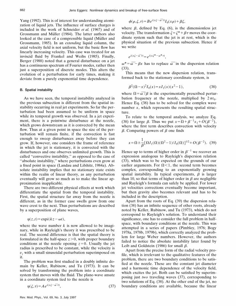
882 Jens Eggers: Nonlinear dynamics and breakup of free-surface flows
Yang (1992). This is of interest for understanding atomi-zation of liquid jets. The influence of surface charges isincluded in the work of Schneider et al. (1967) and ofGrossmann and Muller (1984). The latter authors alsolooked at the case of a compressible liquid (Muller andGrossmann, 1985). In an extending liquid column, theaxial velocity field is not uniform, but the basic flow haslinearly increasing velocity. This case was treated for aninviscid fluid by Frankel and Weihs (1985). Finally,Berger (1988) noted that a general disturbance on a jethas a continuous spectrum of Fourier modes, rather thenjust a superposition of discrete modes. This alters theevolution of a perturbation for early times, making itdeviate from a purely exponential time dependence.
B. Spatial instability
As we have seen, the temporal instability analyzed inthe previous subsection is different from the spatial in-stability occurring in real jet experiments. So far the per-turbation had been assumed to be uniform in spacewhile its temporal growth was observed. In a jet experi-ment, there is a pointwise disturbance at the nozzle,which grows downstream as it is convected by the meanflow. Thus at a given point in space the size of the per-turbation will remain finite, if the convection is fastenough to sweep disturbances away before they cangrow. If, however, one considers the frame of referencein which the jet is stationary, it is convected with thedisturbances and one observes unlimited growth. This iscalled ‘‘convective instability,’’ as opposed to the case of‘‘absolute instability,’’ where perturbations even grow ata fixed point in space (Landau and Lifshitz, 1984a). Ab-solute instability implies that no stationary state existswithin the realm of linear theory, as any perturbationeventually will grow so much as to make the linear ap-proximation inapplicable.
There are two different physical effects at work whichdifferentiate the spatial from the temporal instability.First, the spatial structure far away from the nozzle isdifferent, as in the former case swells grow from onewave crest to the next. Thus perturbations are describedby a superposition of plane waves,
h~z ,t !5expi~kz2vt !,
where the wave number k is now allowed to be imagi-nary, while in Rayleigh’s theory it was prescribed to bereal. The second difference is that the spatial theory isformulated in the half-space z.0, with proper boundaryconditions at the nozzle opening z50. Usually the jetradius is prescribed to be constant, while the velocity isv j with a small sinusoidal perturbation superimposed onit.
The problem was first studied in a doubly infinite do-main by Keller, Rubinow, and Tu (1973). It can besolved by transforming the problem into a coordinatesystem that moves with the fluid. The plane-wave ansatzin a coordinate system tied to the nozzle is
h~z ,t!5Aei~xz2v t!, (37)
Rev. Mod. Phys., Vol. 69, No. 3, July 1997
f~r ,z ,t!5Bei~xz2v t!I0~xr!1bz ,
where b , defined by Eq. (6), is the dimensionless jetvelocity. The transformation z5z* 1bt moves the coor-dinate system such that the jet is at rest, which is thephysical situation of the previous subsection. Hence ifwe write
ei~xz2v t!5ei~xz* 2v* t!,
v* 5v 2bx has to replace v in the dispersion relation(33).
This means that the new dispersion relation, trans-formed back to the stationary coordinate system, is
b2~V2x !2I0~x !5xI1~x !~x221 !, (38)
where V5v /b is the experimentally prescribed pertur-bation frequency at the nozzle, multiplied by 2pt0.Hence Eq. (38) has to be solved for the complex wavenumber x , which represents the resulting spatial struc-ture.
To relate to the temporal analysis, we analyze Eq.(38) for large b . Thus we put x5V1b21x11O(b22),where the first term describes convection with velocityb . Comparing powers of b one finds
x5V61b
@VI1~V!~V221 !/I0~V!#1/21O~b22!. (39)
Hence up to terms of higher order in b21 we recover anexpression analogous to Rayleigh’s dispersion relation(33), which was to be expected on the grounds of ourearlier arguments. For V,1, the second term becomescomplex, corresponding to an exponentially growingspatial instability. In typical experiments, b is largerthan 10, so that terms of higher order in b are negligibleand Rayleigh’s formula can safely be applied. For lowerjet velocities corrections eventually become important,but then gravity also becomes relevant and has to beincluded in the description.
Apart from the roots of Eq. (39) the dispersion rela-tion (38) has an infinite sequence of other roots, alreadynoted by Keller, Rubinow, and Tu (1973), which do notcorrespond to Rayleigh’s solution. To understand theirsignificance, one has to consider the full problem in half-space, with boundary conditions at the nozzle. This wasattempted in a series of papers (Pimbley, 1976; Bogy1978a, 1978b, 1979b), which correctly analyzed the prob-lem for large Weber numbers. However, the authorsfailed to notice the absolute instability later found byLeib and Goldstein (1986) for small b .
Apart from the precise form of the radial velocity pro-file, which is irrelevant to the qualitative features of theproblem, there are two boundary conditions to be satis-fied at the nozzle. These are the constant jet diameterand a harmonic time dependence of the velocity field,which excites the jet. Both can be satisfied by superim-posing just two traveling waves (37), corresponding totwo solutions of Eq. (38). At the other end of the jet, noboundary conditions are available, because the linear

883Jens Eggers: Nonlinear dynamics and breakup of free-surface flows
approximation will eventually break down as distur-bances grow. They have to be replaced by physical con-ditions on the propagation properties of outgoing solu-tions. One condition is that for a particular branch ofsolutions the wave number must go to zero as V→0,which is obviously the case for the solutions of Eq. (39).This requirement simply means that in a steady state atime-independent boundary condition cannot produce aspatial structure. Expansion of Eq. (38) for small Vshows that precisely two such solutions exist for V→0,so one ends up with the correct number of boundaryconditions at the nozzle.
However, following the two physical branches to largeV , one finds that they correspond to disturbances withdiverging speeds of propagation ]V/]Re( x ) as V→` .This would mean that energy is transported at arbitrarilyhigh speeds, which is also excluded on physical grounds.Only for b>bc51.77 does each solution intersect withanother branch of solutions of Eq. (38), which has thecorrect physical behavior for V→` . Thus steady-statesolutions of the linear problem exist for b>bc . On theother hand, no steady state solution exists for b,bc ,the region of absolute instability found by Leib andGoldstein (1986).
Bogy (1978a) advanced similar arguments, but usedthe existence of a positive group velocity as a criterionto select physical branches. However, Leib and Gold-stein (1986) have shown that negative group velocities infact do exist even in the stationary state. These authorssolved the linear problem directly by studying the nozzleproblem in much greater detail. In particular, theylooked at the influence of different velocity profiles atthe nozzle lip, which typically is a Hagen-Poiseuille pro-file, as opposed to the plug profile analyzed above. Forthe Hagen-Poiseuille profile the critical jet velocity iseven lower, so the issue of absolute instability in jet de-cay will probably remain an interesting, albeit somewhatacademic problem, as gravity will always interfere.
C. Higher-order perturbative analysis
Starting from the result of linear theory, the simplestway to explore nonlinear effects is to extend Rayleigh’sanalysis to higher order in the small-amplitude e . Thefirst such analysis was due to Bohr (1909), who studiedthe stable oscillations a jet performs around its equilib-rium shape if it is released from an orifice with a noncir-cular cross section. In the following, we are going toconcentrate on the axisymmetric case, which is muchmore difficult, for both stable and unstable ranges ofwave numbers exist. As a result, the expansions cannotbe expected to be uniformly valid for all wave numbers.
For short-wavelength perturbations, against which theinterface is stable, perturbation theory is the obviousway to include nonlinear effects, as the perturbationsremain bounded. Hence one can expect to obtain solu-tions that are uniformly valid in time. For unstable per-turbations, however, the perturbation solutions are validonly for short times, because higher-order terms haveincreasingly fast growth rates. This is not very surprising,
Rev. Mod. Phys., Vol. 69, No. 3, July 1997
as the time scale t05(rr03/g)1/2, on which the linear so-
lution is evolving is of the same order as the breakuptime. But obviously the dynamics close to the equilib-rium solution do not know about the behavior nearbreakup, so the solution breaks down when the pertur-bation is of the same order as the radius itself. So for adescription of drop formation other methods areneeded. However, there is some hope that as long as theperturbations are small, the nonlinear analysis might de-scribe the growth of higher-order harmonics, which areautomatically excited through the nonlinear interaction.If the perturbation expansion is carried out to third or-der, it will give some indication of the nonuniformbreakup of a liquid jet, which produces smaller satellitedrops in between the main drops.
The first such theory was attempted by Yuen (1968).The primary prediction of his work is that the boundarybetween stable and unstable wave numbers is shifted tolarger values, as compared to Plateau’s result kr051, ifthe perturbations have finite amplitude. Thus perturba-tions that are linearly stable may be unstable because ofnonlinear effects. To find this stability boundary, it issufficient to treat the case of stable oscillations. In theregion of unstable wave numbers, the perturbation ex-pansions are far from rigorous. In particular, the coeffi-cients have singularities at ‘‘resonant’’ wave numbers ofkr051/2 and possibly others, which are not understood.For that reason, we shall focus on the issue of the non-linear stability boundary, which is a highly nontrivialproblem in itself and has been the subject of some con-troversy.
Nayfeh (1970) showed that Yuen’s treatment of thestability boundary was incorrect, predicting an evenlower cutoff wave number. Subsequently, Lafrance(1975) published a theory that predicted no shift in thecutoff at all. This apparent discrepancy was later tracedback to an error in his algebra (Chaudhary and Rede-kopp, 1980). Since the origin of these discrepancies havenever been satisfactorily cleared up, we shall give anexposition of the essential features of the theory. Belowwe show that Nayfeh’s (1970) result xc5113e2/4 for thestability boundary is recovered by modifying Yuen’s(1968) original analysis. In the next section this resultwill also be tested by computer simulation on a one-dimensional simplified model (Eggers, 1995b).
To proceed, one writes the velocity potential and thesurface deformation as a power series in e :
f~r ,z ,t!5(i51
`
e if i~r ,z ,t!,(40)
h~z ,t!5(i51
`
e ih i~z ,t!.
Plugging this into the equations of motion (27) and com-paring powers in e , one generates a closed system ofequations at each order. The boundary terms are evalu-ated by expanding f and h around r51. Thus the equa-tions at nth order have the structure

884 Jens Eggers: Nonlinear dynamics and breakup of free-surface flows
S ]r21
]r
r1]z
2Dfn50,
]thn5]rfn1F$f1 ,h1 , . . . ,fn21 ,hn21%ur51 , (41)
]tfn5hn1]z2hn1G$f1 ,h1 , . . . ,fn21 ,hn21%ur51 ,
where F and G are complicated, but calculable, nonlin-ear functions of the lower-order terms. This allows oneto calculate f i and h i recursively to any order.
Owing to the nonlinear interactions between modes,increasingly higher harmonics of cos(xz) will be gener-ated, up to cos(nxz) at nth order. Following Yuen(1968), we shall pursue this procedure to third order,which is where the first corrections to the linear stabilityboundary come in. Corrections of typographical errorsin Yuen’s original work are given in Rutland and Jame-son (1971) and Taub (1976).
The structure of the second- and third-order terms is
h2~h ,t!5A22~t!cos~2xz!1A20~t!, (42)
f2~r ,h ,t!5B22~t!I0~2xr!cos~2xz!1B20~t!,
and
h3~h ,t!5A33~t!cos~3xz!1A31~t!cos~xz!, (43)
f3~r ,h ,t!5B33~t!I0~3xr!cos~3xz!
1B31~t!I0~xz!cos~xz!,
where the coefficients Aij and Bij are complicated func-tions of time and the reduced wave number x (Yuen,1968; Rutland and Jameson, 1971; Taub, 1976). At nthorder, they contain terms cosh(nv t) and sinh(nv t), sothe corresponding perturbation is proportional toenexp(nv t). Thus for unstable wave numbers x,1 theexpansion is valid only for times t!2log(e/v ). If theleading-order perturbation is of order one, which is thecase near breakup, all other contributions will be of or-der one as well. Note also that the coefficients containsingularities at subharmonic values of the cutoff wavenumber. For example, A22(t) has a pole at x51/2.
But even for x.1 the expansion is not uniformly validin time, even though for e→0 the solution should bestable and all coefficients should be bounded. In fact,A31(t) contains so-called secular terms, which grow lin-early in time and thus invalidate the solution for t*e .The reason is that the third-order solution is convectedand stretched by the first-order contribution. This con-dition cannot be represented by harmonics of finite or-der, but rather one needs contributions from all ordersof the perturbation expansion.
One way around this problem is to reparametrize timeand space coordinates according to
t 5nt , (44)
z 5kcz ,
where n511e2n21••• and kc511e2k21••• bothhave expansions in e itself. This procedure, called themethod of strained coordinates (van Dyke, 1975), wasfirst used by Yuen (1968) in the context of the present
Rev. Mod. Phys., Vol. 69, No. 3, July 1997
problem. Organizing the perturbation expansion in thenew variables t and z means one has to replace the dif-ferential operators ]t and ]z by n]t 5(11e2n21•••)]tand kc]z 5(11e2k21•••)]z . By adjusting the free con-stants n2 and k2, one hopes to remove secular terms atthird order. Effectively, one is resumming certain contri-butions from all orders. It is, however, far from trivialthat this resummation procedure works at all orders. Wehave to be content with the third-order results, but shallcheck them against numerical simulations later.
If k2 is nonzero, this implies a shift in the cutoff wavenumber, as cos(xz)5cos(x z ), with x 5x/kc . Thus thegrowth rate is now
v 15F x I1~ x !
I0~ x !~12 x 2!G 1/2
,
which is real for x ,1 or
x,11e2k2 . (45)
In the strained coordinates the equation for A31 ,which contains the secular term, is
]t2A312v 1
2A315P1~ x !cosh(~v 11v 2!t )
1P2~ x !cosh(~v 12v 2!t )
1P3~ x !cosh~3v 1t !
1@P4~ x !1v 12P5~ x !n2
1(v 12P6~ x !2 x 4)k2#cosh~v 1x !, (46)
where
v 2252
I1~2 x !
I0~2 x !x ~124 x 2!.
The particular solution coming from the last contribu-tion contains the secular term
A315t
2v 1
@P4~ x !1v 12P5~ x !n2
1(v 12P6~ x !2 x 4)k2#sinh~v 1x !,
which grows with t unless the terms in the angularbrackets cancel. Yuen used precisely this condition todetermine n2 and k2, setting
n2521
v 12P5~ x !
$P4~ x !1(v 12P6~ x !2 x 4)k2%. (47)
Near the cutoff wave number x 51, this expression has asingularity, since v 1→0. To cancel this singularity oneputs
k25P4~1 !5916
,
which together with Eq. (45) is Yuen’s result for thecutoff wave number.
Yuen overlooked the fact that the termP3( x )cosh(3v 1t) in Eq. (46) produces additional secularterms as v 1→0. That is, since P3(1)53/16, Eq. (46) be-comes at x 51

885Jens Eggers: Nonlinear dynamics and breakup of free-surface flows
]t2A315(P1~1 !1P2~1 !)cosh~v 2t !1
34
2k2 .
This means A315(3/42k2) t 2 up to oscillatory terms.Thus to cancel the secular terms in the cutoff region onehas to put k253/4, and the correct cutoff wave numberbecomes
xc51134
e2. (48)
This result was first found by Nayfeh (1970), using themethod of multiple time scales (Bender and Orszag,1978).
It should be mentioned that the shift predicted by Eq.(48) is extremely small, so that an experimental verifica-tion has not yet been possible. If the perturbation am-plitude is 10% of the radius, the wave number must beknown to within one percent. Even simulations have notled to a significant confirmation (Ashgriz and Mashayek,1995). Therefore we shall test Eq. (48) in the next sec-tion within the framework of one-dimensional models,for which the perturbation theory is virtually identical,except for some differences in the coefficients. The cut-off wave number comes out to be the same.
Away from the cutoff wave number in the unstableregion, the growth of higher-order harmonics has beenmeasured by Taub (1976), using a highly sensitive sur-face probe. Treating the Weber number as a free param-eter, he found good agreement with Yuen’s theory. Ash-griz and Mashayek (1995) also investigated stableoscillations for x.xc , plotting the time dependence ofvarious harmonics of the fundamental perturbation. Noquantitative comparison with nonlinear theories was at-tempted. This welcome test of their validity remains aworthwhile objective. Chaudhary and Redekopp’s(1980) work differed in two ways from previous investi-gations: first, they considered an initial perturbation ofthe velocity field instead of one of the surface. This wasto mimic the true excitations of a jet at the nozzle, whichcouples to the velocity field. Their treatment of the cut-off region was the same as Yuen’s, which means theyalso did not properly take into account the fact that v 1goes to zero as the cutoff is approached. Therefore theirtreatment of the cutoff is subject to the same criticism,and it would be a worthwhile problem to redo theiranalysis. The second aspect of their work was to con-sider the influence of higher-order harmonics in thedriving, which to some extent had also been done byCline and Anthony (1978). Owing to nonlinearities thetwo inputs interact at higher orders and change the evo-lution of the jet. We shall discuss this in greater detail inSec. VII.C on satellite formation.
Finally, we mention the work of Wang (1968), whostudied the effect of finite amplitudes on the most un-stable wave number. He obtained a correction to Ray-leigh’s result xR50.697 which depends on the amplitude.
V. ONE-DIMENSIONAL APPROXIMATIONS
It seems obvious that the three-dimensional equationsdescribing the nonlinear motion of free-surface flow are
Rev. Mod. Phys., Vol. 69, No. 3, July 1997
hopelessly complicated if analytical solutions are to beobtained. Perturbation theory cannot be extended to theregime close to breakup. One is therefore interested ingenerating simplified equations that still capture the es-sential nonlinear physics of the problem. This is possiblein situations where the fluid thread is long and thin, sothat the fluid flow is directed mostly along the axis andthe velocity field is effectively one-dimensional. In par-ticular, this so-called slenderness assumption turns outto be generically valid close to breakup and becomesexact asymptotically close to pinchoff (Eggers, 1993).
Our strategy is to expand the velocity field in the ra-dial direction, whose lowest-order terms should be suf-ficient to describe the radial motion. Equations of mo-tion are then derived for the expansion coefficients,which depend only on the axial variable z . The ideabehind this goes back to Reynolds (1886) and is oftencalled the ‘‘lubrication approximation.’’ This is becauseit is traditionally applied to flows in a narrow channel,for instance between two moving mechanical parts. Inthe direction perpendicular to the surface the velocityfield will be parabolic, leaving an equation for the am-plitude as a function of the position in the channel.
The situation of free-surface flow, however, is muchmore complicated. First, the smallness of the expansionparameter will depend on the solution itself, essentiallyon whether the typical surface height is really small com-pared to a typical longitudinal extension. Second, it isnot obvious which forces in the equations have to betaken into account. In the example of lubrication flow,viscous forces will be balanced by pressure forces, whileinertia is not important. But in our case the relative im-portance of inertial, viscous, or surface-tension forceswill depend on the problem considered. Nevertheless,the lubrication approximation for radially symmetricfree-surface flow by now has some history of its own,inspired partly by the theory of shallow-water waves,summarized by Peregrine (1972). A broad perspectiveon approximations for axisymmetric flows is given inMiddleman’s (1995) book. The beautiful discussion offlows includes jets, waves, drop dynamics, and thin-filmflow. Unfortunately, the lubrication equations for a thinjet, to be derived below, are not given correctly.
Matovich and Pearson (1969), as well as Pearson andMatovich (1969) and Schultz and Davis (1982) derivedequations for the steady motion of viscous threads inorder to study fiber spinning. In a pioneering work, Lee(1974) studied the dynamics of an inviscid liquid jet, in-cluding a fully nonlinear numerical computation. Thisallowed him to look at the nonuniformity of breakupand to estimate the size of satellite drops. Lee’s equa-tions were further investigated (Pimbley, 1976; Pimbleyand Lee, 1977) to study satellite behavior. The funda-mental problem with Lee’s equations is, however, thatviscosity will become important in the process of pinch-ing, regardless of how small. We shall investigate thespurious singularities of the inviscid equations later inmuch greater detail (Brenner et al., 1997).
This problem was fixed by Green (1976), who derivedequations that included viscosity. His approach was dif-

886 Jens Eggers: Nonlinear dynamics and breakup of free-surface flows
ferent from Lee’s, as he did not start from the equationsof motion, but rather from an inherently one-dimensional description, endowed with the correct sym-metry properties (Green and Laws, 1966). We shall seebelow that these so-called Cosserat equations can in factbe obtained from the Navier-Stokes equation by averag-ing over appropriate slices of the fluid (Dupont, 1993).Again, the Cosserat equations were used in a series ofpapers (Bogy, 1978a, 1978b, 1979a, 1979b) focusing onlinear stability, and in numerical simulations (Bogy,Shine, and Talke, 1980; Shield, Bogy, and Talke, 1986).The same equations were also used extensively in thecontext of liquid bridges (Meseguer, 1983; Meseguer andSanz, 1985; Perales and Meseguer, 1992).
But it was not until recently that a systematic deriva-tion of viscous one-dimensional equations was carriedout starting from the Navier-Stokes equation. Bechtel,Forest, and Lin (1992) used a perturbative approach toobtain one-dimensional equations to arbitrarily high or-der, which we shall explain in Sec. V.A. Independently,Eggers and Dupont (1994) and Garcia and Castellanos(1994) gave essentially the same leading-order equa-tions. At higher orders, different approaches are pos-sible. In Sec. V.B we shall explain how the one-dimensional Cosserat equations are obtained from theNavier-Stokes equation.
A. Radial expansion method
We want to find approximate solutions to the equa-tions of motion in a situation where the typical thicknessl r of the fluid neck is small compared with a typicalaxial scale l z . This means the problem contains a smallparameter e which relates the two scales
l r5el z . (49)
In addition to the length scales l r and l z the problem ischaracterized by a time scale t . These scales can now beused to estimate the order of magnitude of the differentterms in the equations of motion. We begin by sayingthat the axial component of the velocity field is approxi-mated by vz'l z /t , which may also be viewed as thedefinition of t . By continuity, we have ]zvz']rvr , andhence vr'el z /t . The motion is driven by surface ten-sion, so the main contribution to the pressure comesfrom the mean curvature, p/r'(g/r)k . For an almostflat interface, k is dominated by the radius of curvatureperpendicular to the axis, and hence k'1/l r andp/r'(g/r)/l r . From the Navier-Stokes equation wehave ] tvz']zp/r , implying that g/r'l rl z
2/t25el z3/t2.
So, if surface tension has this order of magnitude, sur-face tension and inertial forces are balanced.
We have already mentioned that the inviscid equa-tions develop singularities in finite time, so surface ten-sion and inertial forces must also be balanced by viscos-ity for a consistent theory. We expect vz to have thegreatest variations in the z direction, so the dominantviscous term is n]z
2vz'n/(l zt). Equating n/(l zt) with] tvz we find that n'l z
2/t is the viscosity at which vis-cous forces are balanced by inertia.
Rev. Mod. Phys., Vol. 69, No. 3, July 1997
For a given problem, n and g/r are of course givennumbers, so physically speaking the scales l r , l z , andt of a particular solution adjust themselves to make vari-ous terms in the equations balance. For example, toavoid an inviscid singularity, l z and t will come out toensure n'l z
2/t . From the constancy of the physical pa-rameters n and g/r we can therefore deduce thatl z
2'nt and l r'gt/(rn), so we get l z'(n2r/g)e ,l r'(n2r/g)e2, and t'(n3r2/g2)e2. If the typical scalesof a solution behave in this way, surface-tension, inertial,and viscous forces will be balanced during the entireevolution of this solution.
Having estimated the typical size of all terms, it isuseful to choose the scales l z , l r , and t such that
l z5el n , l r5e2l n , and t5e2tn , (50)
with
l n5n2r
g, tn5
n3r2
g2 . (51)
These are the unique length and time scales that can beformed from the material parameters. When we usel z , l r , and t to nondimensionalize all variables accord-ing to
r5l rr , z5l zz , t5t t ,
vr5l r
tv r , vz5
l z
tv z , p/r5
l z2
t2 p , (52)
h5l rh ,
all material parameters drop out of the problem and therescaled equations of motion become
] t v r1 v r] r v r1 v z] z v r521e2 ] r p 1
1e2 ] r
2v r1] z2v r
11e2 ] r v r / r 2
1e2 v r / r 2,
(53)
] t v z1 v r] r v z1 v z] z v z52] z p 11e2 ~] r
2v z1] r v z / r !
1] z2v z .
The equation of continuity is
] r v r1] z v z1 v r / r 50, (54)
and the tangential and normal force balances read
p 22
11e2~] z h !2@] r v r1e2] z v z~] z h !2
2~] r v z1e2] z v r!] z h #5k u r 5h , (55)
2e2~] r v r2] z v z!] z h 1~] r v z1e2] z v r!(12e2~] z h !2)
50u r 5h .
Finally, the kinematic boundary condition is
] t h 1 v z] z h 5 v ru r 5h . (56)
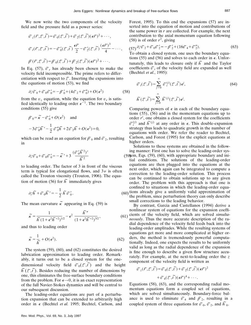
887Jens Eggers: Nonlinear dynamics and breakup of free-surface flows
We now write the two components of the velocityfield and the pressure field as a power series:
v z~ r , z , t !5 v 0~ z , t !1 v 2~ z , t !~e r !21••• ,
v r~ r , z , t !52 v 08~ z , t !e r
22 v 28~ z , t !
~e r !3
42••• , (
p ~ r , z , t !5p 0~ z , t !1p 2~ z , t !~e r !21••• .
In Eq. (57), v r has already been chosen to make thevelocity field incompressible. The prime refers to differ-entiation with respect to z . Inserting the expansions intothe equations of motion (53), we find
] t v 01 v 0v 0852p 081~4 v 21 v 09!1O~e2! (58)
from the vz equation, while the equation for vr is satis-fied identically to leading order e21. The two boundaryconditions (55) give
p 05k 2 v 081O~e2! and
23 v 08h 8212
v 09h 12 v 2h 1O~e2!50,
which can be read as an equation for p 0 and v 2, resultingin
] t v 01 v 0v 0852k 813~ v 08h 2!8
h 2(59
to leading order. The factor of 3 in front of the viscousterm is typical for elongational flows, and 3n is oftencalled the Trouton viscosity (Trouton, 1906). The equa-tion of motion (56) for h immediately gives
] t h 1 v 0h 85212
h v 08 . (60)
The mean curvature k appearing in Eq. (59) is
k 51
h ~11e2h 82!1/22e2
h 9
~11e2h 82!3/2, (61)
and thus to leading order
k 51
h1O~e2!. (62)
The system (59), (60), and (62) constitutes the desiredlubrication approximation to leading order. Remark-ably, it turns out to be a closed system for the one-dimensional velocity field v 0( z , t ) and the heighth ( z , t ). Besides reducing the number of dimensions byone, this eliminates the free-surface boundary conditionsfrom the problem. For e→0, it is an exact representationof the full Navier-Stokes dynamics and will be central toour subsequent discussion.
The leading-order equations are part of a perturba-tion expansion that can be extended to arbitrarily highorder in e (Bechtel et al. 1995; Bechtel, Carlson, and
Fstc(
Tttc(
CtovseCh
ittenccoctts
ncndledtvirc
Emwac
Rev. Mod. Phys., Vol. 69, No. 3, July 1997
57)
)
orest, 1995). To this end the expansions (57) are in-erted into the equation of motion and contributions ofhe same power in r are collected. For example, the nextontribution to the axial momentum equation following58) is of order r2, giving
] t v 21 v 0v 2852p 281~16v 41 v 29!. (63)
o obtain a closed system, one uses the boundary equa-ions (55) and (56) and solves to each order in e . Unfor-unately, this leads to closure only if h and the Tayloroefficients v i of the velocity field are expanded as wellBechtel et al., 1995):
v i~ z , t !5(j50
`
v i~ j !~ z , t !e j, (64)
h ~ z , t !5(j50
`
h ~ j !~ z , t !e j.
omparing powers of e in each of the boundary equa-ions (55), (56) and in the momentum equations up torder ri, one obtains a closed system for the coefficients˜ i
(j) and h (j) at any order in e . This double-expansiontrategy thus leads to quadratic growth in the number ofquations with order. We refer the reader to Bechtel,arlson, and Forest (1995) for the explicit equations atigher orders.Solutions to these systems are obtained in the follow-
ng manner: First one has to solve the leading-order sys-em, Eqs. (59), (60), with appropriate boundary and ini-ial conditions. The solutions of the leading-orderquations are then plugged into the equations at theext order, which again can be integrated to compute aorrection to the leading-order solution. This processan be continued to obtain solutions up to any givenrder. The problem with this approach is that one isonfined to situations in which the leading-order equa-ions already give a uniformly valid approximation ofhe problem, since perturbation theory can only describemall corrections to the leading behavior.
By contrast, Garcia and Castellanos (1994) derive aonlinear system of equations for the expansion coeffi-ients of the velocity field, which are solved simulta-eously. Thus the more accurate description of the ra-ial dependence of the velocity field feeds back into the
eading-order amplitudes. While the resulting systems ofquations get more and more complicated at higher or-ers, the method is tremendously powerful computa-ionally. Indeed, one expects the results to be uniformlyalid as long as the radial dependence of the expansions fine enough to describe a given flow structure accu-ately. For example, at the next-to-leading order the zomponent of the velocity field is written as
v z~ r , z , t !5 v 0~ z , t !1 v 2~ z , t !~e r !2
1 v 4~ z , t !~e r !41••• .
quations (58), (63), and the corresponding radial mo-entum equations form a coupled set of equations,hich are solved simultaneously. Boundary-force bal-nce is used to eliminate v 4 and p 2, resulting in aoupled system of three equations for v 0, v 2, and h 0.

888 Jens Eggers: Nonlinear dynamics and breakup of free-surface flows
B. Averaging method: Cosserat equations
In this subsection, we describe an entirely differentapproach to obtaining one-dimensional approximations,based on integrating the equations of motion over a sliceof the fluid. Interestingly, the leading-order versions ofthis procedure lead to a set of equations well known asthe Cosserat equations (Green, 1976). In an approachborrowed from solid mechanics (Green and Laws, 1966),one starts from a system of one-dimensional fields,called ‘‘directors.’’ The equations of motion are then de-rived from symmetry considerations and conservationproperties and they coincide with the equations derivedfrom the Navier-Stokes equation by integrating overslices. Ultimately, this is not surprising, as the momen-tum over a slice of the fluid must inherit the correctsymmetry properties from the full equations of motion.The obvious advantage of this derivation (Dupont,1993), presented here for the first time, is that there is aclear connection to the three-dimensional equations ofmotion. Therefore the error made at a given order of theapproximation can be estimated and can be systemati-cally improved by going to a higher order of the ap-proximation. Methods that are very similar in spirit, butlead to a coupled set of integro-differential equations,have been developed by Entov and Yarin starting fromthe early 1980s (Yarin, 1993) and by Dewynne, Howell,and Wilmott (1994). They are more general in that theyallow for an arbitrary position of the centerline of the jetas well as noncircular cross sections.
Dupont’s procedure is essentially a Galerkin approxi-mation of the equations of motion, which means the ve-locity is represented by a superposition of a finite num-ber of basis functions. Equations of motion for thecoefficients are obtained by projecting the Navier-Stokes equation onto each of the basis functions. Again,a coupled system of equations results, which should rep-resent the velocity field more and more accurately athigher orders.
The basis functions used represent slices of the fluid,
w~2i , z !~r ,z !5S 2r2i11
2i12d8~z2 z !
r2id~z2 z !
D , (65)
which are divergence free, with a discrete index i and acontinuous index z representing the position of the slice.The main deficiency of the functions (65) is that they arenot orthogonal for different i , which is the price one hasto pay for their being both perfectly localized in spaceand divergence free. Using Eq. (65), we can write anyincompressible velocity field as a unique superpositionof basis functions:
v~r ,z ,t !5(i50
` E2`
`
v ~2i !~ z ,t !w~2i , z !~r ,z !dz . (66)
Now one has to plug Eq. (66), truncated at some or-der i5n , into the Navier-Stokes equation and the kine-matic boundary condition and project it onto the corre-
Rev. Mod. Phys., Vol. 69, No. 3, July 1997
sponding n11 basis functions w(2i , z )(r ,z),i50, . . . ,n .This yields a coupled set of (n12) equations for theamplitudes v(0)( z ,t), . . . ,v(2n)( z ,t), and h( z ,t). Toproject the Navier-Stokes equation onto an arbitrary in-compressible vector field w(r ,z), we write it in the form
r(] tv1~v¹!v)5“•s, (67)
where the stress tensor is given by
s ij52pd ij12hDij~v! (68)
and
Dij~v!512
~] jv i1] iv j! (69)
is the deformation tensor. We multiply the Navier-Stokes equation by w(r ,z) and integrate over the vol-ume of the fluid, 0<r<h(z). The result can be writtensymbolically as
rIr5Is ,
where
Ir5EV
@] tv1~v¹!v#wd3x and
Is5EV
~¹s!wd3x . (70)
On integrating by parts, Is can be written as
Is5EV
] is ijwjd3x52E
Vs ij] iwjd
3x
1E]V
nis ijwjd2s .
In the first integral on the right the pressure does notcontribute, since ] iwi50. For the second integral we usethe force balance at the boundary,
nis ij52gknj .
Thus after some manipulations we obtain
Is522hIh2gIg ,
where
Ih5EV
Dij~v!Dij~w!d3x , Ig5E]V
k~nw!d2s ,
and the desired projection of the Navier-Stokes equa-tion is in full
rEV
@] tv1~v¹!v#wd3x52gE]V
k~nw!d2s
22hEV
Dij~v!Dij~w!d3x .
(71)
To be more explicit, we compute the leading-orderapproximation, so
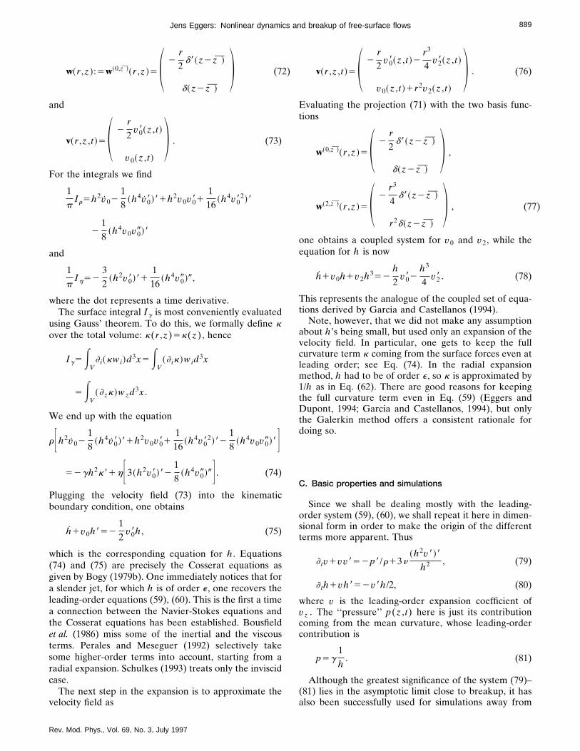
889Jens Eggers: Nonlinear dynamics and breakup of free-surface flows
w~r ,z !:5w~0,z !~r ,z !5S 2r
2d8~z2 z !
d~z2 z !
D (72)
and
v~r ,z ,t !5S 2r
2v08~z ,t !
v0~z ,t !D . (73)
For the integrals we find
1p
Ir5h2v0218
~h4v08!81h2v0v081116
~h4v082!8
218
~h4v0v09!8
and
1p
Ih5232
~h2v08!81116
~h4v09!9,
where the dot represents a time derivative.The surface integral Ig is most conveniently evaluated
using Gauss’ theorem. To do this, we formally define kover the total volume: k(r ,z)5k(z), hence
Ig5EV
] i~kwi!d3x5EV
~] ik!wid3x
5EV
~]zk!wzd3x .
We end up with the equation
rFh2v0218
~h4v08!81h2v0v081116
~h4v082!82
18
~h4v0v09!8G52gh2k81hF3~h2v08!82
18
~h4v09!9G . (74)
Plugging the velocity field (73) into the kinematicboundary condition, one obtains
h1v0h85212
v08h , (75)
which is the corresponding equation for h . Equations(74) and (75) are precisely the Cosserat equations asgiven by Bogy (1979b). One immediately notices that fora slender jet, for which h is of order e , one recovers theleading-order equations (59), (60). This is the first a timea connection between the Navier-Stokes equations andthe Cosserat equations has been established. Bousfieldet al. (1986) miss some of the inertial and the viscousterms. Perales and Meseguer (1992) selectively takesome higher-order terms into account, starting from aradial expansion. Schulkes (1993) treats only the inviscidcase.
The next step in the expansion is to approximate thevelocity field as
Rev. Mod. Phys., Vol. 69, No. 3, July 1997
v~r ,z ,t !5S 2r
2v08~z ,t !2
r3
4v28~z ,t !
v0~z ,t !1r2v2~z ,t !D . (76)
Evaluating the projection (71) with the two basis func-tions
w~0,z !~r ,z !5S 2r
2d8~z2 z !
d~z2 z !
D ,
w~2,z !~r ,z !5S 2r3
4d8~z2 z !
r2d~z2 z !
D , (77)
one obtains a coupled system for v0 and v2, while theequation for h is now
h1v0h1v2h352h
2v082
h3
4v28 . (78)
This represents the analogue of the coupled set of equa-tions derived by Garcia and Castellanos (1994).
Note, however, that we did not make any assumptionabout h’s being small, but used only an expansion of thevelocity field. In particular, one gets to keep the fullcurvature term k coming from the surface forces even atleading order; see Eq. (74). In the radial expansionmethod, h had to be of order e , so k is approximated by1/h as in Eq. (62). There are good reasons for keepingthe full curvature term even in Eq. (59) (Eggers andDupont, 1994; Garcia and Castellanos, 1994), but onlythe Galerkin method offers a consistent rationale fordoing so.
C. Basic properties and simulations
Since we shall be dealing mostly with the leading-order system (59), (60), we shall repeat it here in dimen-sional form in order to make the origin of the differentterms more apparent. Thus
] tv1vv852p8/r13n~h2v8!8
h2 , (79)
] th1vh852v8h/2, (80)
where v is the leading-order expansion coefficient ofvz . The ‘‘pressure’’ p(z ,t) here is just its contributioncoming from the mean curvature, whose leading-ordercontribution is
p5g1h
. (81)
Although the greatest significance of the system (79)–(81) lies in the asymptotic limit close to breakup, it hasalso been successfully used for simulations away from
890 Jens Eggers: Nonlinear dynamics and breakup of free-surface flows
breakup (Eggers and Dupont, 1994; Brenner, Shi, andNagel, 1994). The key to this success lies in a modifica-tion of Eq. (81) to include the complete expression forthe mean curvature,
p5gS 1h~11h82!1/2 2
h9
~11h82!3/2D . (82)
This procedure was already adopted by Lee (1974), andhas subsequently been used by many other authors (Me-seguer, 1983; Johnson et al., 1991; Garcia and Castell-anos, 1994). The best rationale for doing so is offered bythe Galerkin procedure of the previous subsection, butEq. (79) has the advantage of much greater mathemati-cal simplicity over Eq. (74). The complete curvature onthe right-hand side of Eq. (82) is of course also repre-sented as an infinite sequence of terms in the equationsof the radial expansion. It would be extremely desirableto develop a general and consistent method to ‘‘resum’’all the relevant terms of the expansion, such that Eq.(82) is included even at leading order. Perturbative re-summation like this is customary in quantum fieldtheory (Amit, 1978), but has not yet been explored inthe context of nonlinear partial differential equations.
The system (79),(80) has to be supplemented withboundary conditions
h~z6 ,t !5h6~ t !, (83)
v~z6 ,t !5v6~ t !,
where the two boundary points z1 , z2 may themselvesbe time dependent. In a liquid-bridge experiment, forexample, z6 represent the position of the two ringsholding the bridge.
The two most important conservation laws are conser-vation of mass and energy,
] tV5ph2vuz5z2
z1 , (84)
with the volume being
V5pEz2
z1
h2dz , (85)
expressing conservation of mass. The kinetic energy is
Ekin5p
2rE
z2
z1
h2v2dz , (86)
while the potential energy is g times the total surfacearea:
Epot52pgEz2
z1
h~11h82!1/2dz . (87)
Thus the sum obeys the balance equation
] t~Ekin1Epot!5D1boundary terms, (88)
where D is the rate of energy dissipation,
D523pnrEz2
z1
~hv8!2dz . (89)
This means that apart from driving through boundaryterms, the total energy of the system can only decrease,
Rev. Mod. Phys., Vol. 69, No. 3, July 1997
and a drop eventually has to reach some static equilib-rium shape, corresponding to a minimum of the poten-tial energy. Since the potential energy (87) is the same asin the full equations, the physical equilibrium states suchas those of a drop hanging from a faucet (Michael andWilliams, 1976), will also be reproduced exactly. For re-producing the equilibrium states it is of course crucial tokeep the full curvature term as in Eq. (82).
Another important benefit of the ‘‘resummed’’ formof the pressure, Eq. (82), emerges when considering thelinear stability around a cylindrical surface h5r0. Inanalogy to the three-dimensional case [cf. Eq. (31)], wewrite
h~z ,t !5r0@11e cosh~vt !cos~kz !# , (90)
v~z ,t !5ev0 sinh~vt !sin~kz !
and linearize in e . A calculation analogous to that of thefull problem leads to the dispersion relation (34). As wehave mentioned before, this dispersion relation accu-rately approximates the true growth rates for all v . Evenmore important, the stability boundary is at kr051, thesame as for the full equations. This means short-wavelength perturbations will not grow, in contrast tothe leading-order equation (81), which produces infinitegrowth rates for the inviscid problem and still producesfinite growth rates in the limit k→` for finite viscosity(Forest and Wang, 1990). Thus the leading-order systemis unstable against very-short-wavelength ‘‘noise,’’ mak-ing it ill suited for numerical purposes. If one includeshigher-order terms perturbatively (Bechtel, Carlson, andForest, 1995) the problem is not mended, since theleading-order equations are unaffected by higher-orderones.
Linear stability has also been investigated for varioushigher-order models such as the Cosserat equations(Bogy, 1979b) and the parabolic approximation (Garciaand Castellanos, 1994). The dispersion relation of thesemodels still improves the comparison with Rayleigh’sformula. For example, for the Cosserat equation therelative error in the growth rate is less than 0.25% for allunstable wave numbers.
Even using a system that is linearly stable againstshort-wavelength perturbations, numerical simulationsof the fully nonlinear behavior are by no means trivial.This is true in particular in the neighborhood of thepinch point, which is characterized by very small lengthand time scales, and a blowup of the velocity. Theasymptotic behavior near pinchoff described in the nextsubsection sets in only when hmin&l n/205n2r/(20g).Therefore, to simulate the motion of a drop of waterfalling from a 1 cm nozzle, one needs to resolve 8 ordersof magnitude in the minimum height. Moreover, low-viscosity fluids are characterized by steep gradients,which have to be resolved carefully and are likely tocause numerical instabilities.
One can only hope to reach sufficient spatial resolu-tion when the grid is locally refined near the singularity.Since the singularity moves in space and resolution re-quirements cannot be foreseen, the grid has to be ad-

891Jens Eggers: Nonlinear dynamics and breakup of free-surface flows
justed to meet certain accuracy requirements. To ensuresufficient temporal resolution, the time step has to bedynamically adjusted as well. Finally, a solution that in-corporates spatial and temporal scales over many ordersof magnitude, will also be prone to numerical instabili-ties. These have to be dealt with using implicit methods(Press et al., 1992).
The first fully nonlinear calculation is due to Lee(1974), who integrated the lubrication equations (79),(80), and (82) with zero viscosity and using periodicboundary conditions. A more extensive numerical studyof the Cosserat equations (74), (75) in the inviscid andthe viscous case was performed by Bogy, Shine, andTalke (1980). Like Lee, they used finite-difference equa-tions, studied explicit as well as implicit methods, anddiscussed their stability. By contrast, Schulkes (1993)used finite-element methods to compare various inviscidmodels, namely, the full potential-flow equations (9)–(11), the inviscid Cosserat equations, and Lee’s model.He found considerable differences between the threecases, probably due to the fact that inviscid models be-come inconsistent even before breakup occurs, as shownby Eggers and Dupont (1994).
The first quantitative comparison of a one-dimensional model with experiment was carried out byEggers and Dupont (1994), who also included a detailedanalysis of the pinch singularity. To do that, they used asecond-order finite-difference scheme with a highly non-uniform mesh, which was adapted to the solution. Thetime integration was a fully implicit second-orderscheme with adaptive step size control. It forced them tosolve a nonlinear system of equations at each time step,which they did using Newton’s method. A fully implicitscheme was found to be essential in order to controlnumerical instabilities. Figure 15 shows a comparison ofthe numerical computations by Eggers and Dupont witha drop of water at the bifurcation point. The photographis the same as Fig. 10, in which the comparison is with apotential flow simulation.
The lubrication model correctly predicts the globalshape, as it does the drop size, the length of the neck,and the profile near the bifurcation point. This only be-comes possible if one goes beyond the asymptoticmodel, Eqs. (79)–(81), and includes the higher-ordercorrections, [Eq. (82)] in the curvature, such that spheri-cal drops become an equilibrium shape. The model de-veloped by Eggers and Dupont (1994) has also beenused in an extensive study of the nonlinear evolution ofa liquid bridge (Zhang, Padgett, and Basaran, 1996).Again, excellent agreement with experiment was found.
The numerical code originally developed by Eggersand Dupont has been subsequently refined in severaldirections. Shi, Brenner, and Nagel (1994) used a dy-namically evolving grid, which introduced local refine-ment once specified conditions on the solution are met.In the case of low viscosities, treated by Brenner et al.(1997), special care had to be taken, since lack of viscousdamping made the solution sensitive to perturbations.Moreover, steep gradients of the height and the velocityfield occured even before hmin went to zero. These had
Rev. Mod. Phys., Vol. 69, No. 3, July 1997
to be dealt with by introducing additional refinement inregions of large gradients. The sensitivity to noise wasaccounted for by introducing a smooth mesh, whose gridsizes were continuously varied, as opposed to the grad-ing in steps of two used by Eggers and Dupont. Througha combination of all of the above precautions, Brenneret al. (1997) dealt with a Reynolds number correspond-ing to a fluid 1/10 of the viscosity of water, falling from a1 cm nozzle. To fully resolve this problem, the solutionhad to be followed through 10 orders of magnitude inthe minimum height, while the slope reached a maxi-mum of 2000.
To be able to follow up on the evolution afterbreakup, Brenner et al. (1997) also developed a numeri-cal scheme to cut the computational domain into twohalves. Once some minimum thickness was reached,typically 1023 times the initial thickness, the interfacewas extrapolated to a spherical cap on either side andadditional grid points were introduced up to their tips.The two parts of the solution then evolved indepen-
FIG. 15. The same photograph as in Fig. 10, compared withthe lubrication equations of this section (Eggers and Dupont,1994). The lines represent the profile at time distances of0.4(r0
3r/g)1/2 and at the time of pinchoff.

892 Jens Eggers: Nonlinear dynamics and breakup of free-surface flows
dently. By using different threshold thicknesses, theywere able to confirm that the subsequent evolution wasnot affected by the details of the breakup on scaleslarger than the threshold thickness. Brenner et al. (1997)also tested the validity of the lubrication equations afterbreakup, by comparing numerical and experimental pro-files before and after the bifurcation of a drop of waterfalling from a faucet. They found that excellent agree-ment persisted to times after breakup.
By using the high-resolution numerical codes, it is alsointeresting to repeat the nonlinear stability analysis ofSec. IV.C for the one-dimensional equations (Eggers,1995b). The algebra is very similar, and in particular thenonlinear stability boundary (48) comes out to the samevalue, at least up to third order in perturbation theory.To test it numerically, a cylindrical column of fluid withperiodic boundary conditions was set up, with a smallsinusoidal perturbation imposed on it. As usual, alllengths were measured in units of the unperturbed ra-dius. Thus the initial conditions were
h~z ,0!5R2e cos~xz !, (91)
R5~12e2/2!1/2,
which conserves volume independent of e . The totallength of the column was 0<z<2p/x , corresponding toone wavelength. The velocity was zero initially. SinceEq. (48) is only valid for inviscid flow, we applied theextremely large Reynolds number Re510 000, so viscos-ity could be neglected. The perturbation amplitude waschosen to be between 0.01 and 0.1, to make perturbationtheory applicable. The resolution of 50 000 grid pointswas selected to safely resolve wave numbers to 0.01%.
Figure 16 shows the largest unstable wave number as
FIG. 16. Comparison between a numerical simulation of theone-dimensional lubrication equations and nonlinear stabilitytheory. The stability boundary xc in the reduced wave numberis plotted against the perturbation amplitude e . The numericalsimulations clearly confirm Nayfeh’s (1970) theory.
Rev. Mod. Phys., Vol. 69, No. 3, July 1997
diamonds and the smallest stable one as crosses. Theresolution is so high that they cannot be distinguished onthe scale of the plot. The full line is the prediction ofNayfeh’s (1970) theory, the dashed line representsYuen’s (1968) theory. Lafrance’s (1975) work wouldpredict no shift in the critical wave number. Clearly, thevalidity of Nayfeh’s theory near the cutoff is confirmedspectacularly. For e*0.05 theory systematically underes-timates the cutoff value, a result, presumably, of higher-order effects in e .
D. Inviscid theory and conservation laws
In this subsection we shall discuss the fascinating con-nections of the one-dimensional equations with thetheory of integrable systems (Hoppe, 1992). These con-nections are found most elegantly if the equations aretransformed to a Langrangian frame of reference. Let bbe the position of a particle at time t50 or, alterna-tively, and of a slice of fluid of width db . Because themotion is one dimensional and volume is conserved, thesame slice, after being convected to a position z(b ,t),will have the thickness (h2(b ,0)/h2(z ,t))db . Thus weobtain
zb5h2~b ,0!
h2(z~b ,t !,t), (92)
where z(b ,t) is the position at time t of the particleoriginally at b . Subscripts refer to differentiation withrespect to the variable. By changing the labeling accord-ing to da5h2(b ,0)db , we can write Eq. (92) as
za5h22(z~a ,t !,t), (93)
where da is the volume of the slice a . Equation (93) isthus a direct consequence of the volume of fluid ele-ments being conserved. From the definition of z we have
zt5v(z~a ,t !,t). (94)
Making use of the transformation ]z5za21]a , Eqs. (93)
and (94) allow us to rewrite the equation of motion, Eq.(79), in terms of z(a ,t) alone:
ztt521r
]ap(z~a ,t !)za
13nzaS zta
zaD
a
. (95)
The equation for h , Eq. (80), is automatically satisfiedowing to the definition of z(a ,t). If p is replaced by itsleading-order estimate (81), we have simply
ztt52g
2r
zaa
za3/2 13nS zta
za2 D
a
. (96)
Thus the coupled set of equations (79), (80) has beencondensed into a single equation for z(a ,t), which is ofsecond order in time. If one leaves out the dissipationterm, the equation becomes particularly simple:
ztt2~za21/2!a50, (97)
where the constant g/r has been absorbed by a rescalingof variables. The same system has been studied exten-sively in a paper by Ting and Keller (1990), but in itsoriginal form [Eqs. (79)–(81)], with n set equal to zero.
893Jens Eggers: Nonlinear dynamics and breakup of free-surface flows
We stress that Eq. (97) is unphysical as it stands. Aswe shall see in Sec. VII.B, the inviscid equations displaysingularities even before breakup occurs. Still, certaininvariance properties of the inviscid system could revealthemselves even in the presence of a small amount ofviscosity. In fact, we shall see below that Eq. (97) has aninfinite sequence of independent conservation laws,apart from the obvious candidates of energy and mass.In the same vein, the Euler equation has been the sub-ject of intense scrutiny (Majda, 1991), although it is be-lieved to exhibit unphysical singularities of the vorticity(Grauer and Sideris, 1991; Pumir and Siggia, 1992). Onehopes that the study of these singularities will yield in-formation about high-Reynolds-number turbulence, inparticular the mechanisms behind the energy cascade ofeddies. Geometrical invariants of the Euler equation(Tur and Yanovsky, 1993) are expected to act as con-straints for the almost inviscid motion of turbulent flow.
It is readily seen that Eq. (97) is generated by theLagrangian density
L~za ,zt!5zt2/212za
1/2 . (98)
The canonical momentum variable is p5zt , so one findsfor the Hamiltonian
H5E Fp2
21V~za!Gda , (99)
where in our case we have
V~za!52za1/2 . (100)
We have written the Hamiltonian in the general form(99), since the potential
V~za!52Aza
12g
12g(101)
corresponds to the equations of one-dimensional com-pressible gas dynamics (Landau and Lifshitz, 1984a).These equations are usually written in the form
] tv1vv81p8~r!
rr850,
(102)] tr1~vr!850,
where p(r)5Arg is the pressure and r the density ofthe gas. For the system to be stable one needs Ag.0, sothat the pressure increases with density. A comparisonbetween Eqs. (100) and (101) shows that A521 andg51/2, so the pinching problem corresponds to a newclass of unstable systems, not considered in the realm ofgas dynamics.
From among the many remarkable results (Olver andNutku, 1988) that can be derived for Eq. (97), we men-tion that it can be linearized by means of the Legendretransformation
F~za ,zt!5z2aza2tzt , (103)u5za , v5zt .
This is also known as a Hodograph transformation(Manwell, 1971). A straightforward calculation showsthat Eq. (97) is now equivalent to the linear equation
Rev. Mod. Phys., Vol. 69, No. 3, July 1997
Fuu112
Fvv
u3/2 50, (104)
which has an infinite sequence of exact solutions, asshown below (Olver and Nutku, 1988). So one possibleapproach is to transform the initial conditions of theoriginal problem, Eq. (97), to the Hodograph plane(u ,v) and to solve Eq. (104) there.
Another, completely unexpected property of Eq.(104) is the following: Let Q(u ,v) be a solution of Eq.(104). Then Q(za ,p) is a conserved density of the equa-tions of motion. Conversely, all conserved quantitiescorrespond to solutions of Eq. (104). For example, onecan easily check that the Hamiltonian density
H~u ,v !5Q2~u ,v !5v2/212u1/2
is a solution of the Hodograph equation (104). If onesucceeds in finding other solutions of Eq. (104), otherconservation laws in addition to the obvious ones of en-ergy and momentum conservation will be generated. Aninfinite number of solutions are produced by the recur-sion relation (Hoppe, 1995)
]vQn115nQn ,(105)
da~]uQn11!5nFva]uQn2ua
2u3/2 ]vQnG .
Starting from Q125uv and Q1
15v one generates two in-dependent hierarchies of conservation laws, whose firstmembers are
Q115v ,
Q215v2/212u1/2,
(106)Q3
15v3/314vu1/2,
Q415v4/416v2u1/226u lnu ,
and
Q125uv ,
Q225v2u/222u3/2/3,
(107)Q3
25v3u/324vu3/2/3,
Q425v4u/422v2u3/21u2.
All the conserved quantities
Qi65E Qi
6da
are independent, i.e., they Poisson commute:
$Qi6 ,Qj
6%50. (108)
Note the emergence of logarithmic terms in Eq. (106),which appear in the fourth step of the hierarchy. Thisimplies that the scale invariance
Qi1~a4u ,av !5aiQi
1~u ,v !
of Qi1 is broken for i>4. The same is thus true for the
corresponding solutions z(a ,t), since by virtue of theHodograph transformation (103) each of the quantities

894 Jens Eggers: Nonlinear dynamics and breakup of free-surface flows
Rev. Mod. Phys
TABLE I. The fluid parameters for water, glycerol, and mercury. The values are quoted from Weast(1978). The internal scales l n and tn are calculated from the kinematic viscosity n and from the ratioof surface tension g and density r .
Mercury Water Glycerol
n [cm 2/s] 0.0012 0.01 11.8g/r [cm 3/s2] fluid-air interface 34.7 72.9 50.3l n5n2r/g [cm] 4.231028 1.3831026 2.79tn5n3r2/g2 [s] 1.4310212 1.91310210 0.652
Qi6 generates an exact solution of the nonlinear equa-
tion (97). For example, Q21 corresponds to the solution
z~a ,t !5z02t2/221/a . (109)
In contrast to Eq. (109), the solution derived from Q41
will no longer be scale invariant but contains logarithmicterms, which is a telltale sign of anomalous scaling(Amit, 1978). Unfortunately, Eq. (109) results in aheight h(z ,t) which has a singularity at a finite z for alltimes. In fact, it is a remarkable consequence of the in-finite sequence of conservation laws, Eqs. (106), (107),that no localized pinching solution of the inviscid equa-tions can exist. As we shall explain in more detail in Sec.VII.B, a conserved quantity of sufficiently high orderwould always diverge during pinching, which is inconsis-tent with regular initial data. Thus it is of fundamentalimportance to work in the effect of small amounts ofviscosity, which will eventually destroy the rigorous con-servation properties. On large scales, on the other hand,the motion is still subject to the constraints imposed byEqs. (106), (107), as viscosity is not yet important. Thelimit of small viscosities has also been used to studyshock-wave solutions of inviscid equations, for examplein the case of the equations of one-dimensional elasticity(Dafermos, 1987). It is likely that Eq. (97) would de-velop infinitely sharp gradients as well.
VI. SIMILARITY SOLUTIONS AND BREAKUP
A. Local similarity form
Experimental observations have revealed that free-surface shapes of a given fluid are remarkably similarnear the pinch point, independent of initial conditions.For example, jet breakup at different wavelengths (Fig.4) and under the influence of gravity (Fig. 6) all show aconical tip attached to a sharp front if the fluid is water.For high viscosities (Figs. 5 and 7) the solutions turn outto be threads. So while the outer dimension L of theexperimental setup (say the radius of the nozzle) hardlyseems to matter, there is a strong dependence on viscos-ity. In fact, if L does not enter the description nearbreakup, the only other scale the solution can depend onis the ‘‘inner’’ length scale l n5n2r/g and the corre-sponding time scale tn5n3r2/g2. Thus, when doublingthe viscosity, breakup should look similar when viewedon length scales four times as large and time scales eighttimes as long as already noted by Haenlein (1931).
Some values of l n and tn are shown in Table I for
., Vol. 69, No. 3, July 1997
three common Newtonian fluids. Variations in l n andtn are huge, which is an asset for experiments: just bychoosing different fluids, one can explore a wide rangeof different scaling behaviors. For water, l n is almost onmolecular scales, while for glycerol it is about the sameas typical outer scales. Since the relevant scale of pinch-ing solutions is set by l n and tn , none of the asymptoticscan be seen in the experiments with water, at least at thepresent state of spatial and temporal resolution. It israther the long and skinny threads observed in high-viscosity experiments that are characteristic of the finalstages of pinching.
The solutions close to the pinch point, which we as-sume to be at z0 and at a time t0, depend only on l n andtn . Thus the height and the velocity should be represent-able as
h~z ,t !5l nhs~z8,t8!,
v~z ,t !5l n
tnvs~z8,t8!, (110)
where z85(z2z0)/l n and t85(t02t)/tn measure thedistance from the singularity and hs , vs are universalfunctions. This universality was verified numerically us-ing the lubrication equations (79), (80), and (82) for dif-ferent viscosities and initial conditions (Eggers and Du-pont, 1994).
Near a singularity the flow lacks a typical scale, soself-similarity is a natural concept. Indeed, a self-similarsolution of a flow leading to a singularity was alreadygiven by Guderley (1942) in the case of a sphericalshock wave. Constantin et al. (1993) and Bertozzi et al.(1994) studied the breakup of a fluid drop between twoclosely spaced glass plates using similarity solutions. Inthe context of the present problem, Ting and Keller(1990) studied singular solutions of an inviscid version ofthe lubrication equations (79)–(81). Similarity solutionsof the viscous equations were found by Eggers (1993).
The existence of self-similar solutions of the pinchingproblem is in fact already implicit in the scaling analysisof Sec. V.A. Equation (50) means that the balance ofinertial, surface-tension, and viscous forces is indepen-dent of the parameter e , which measures the minimumthickness of the thread. Thus the leading-order equa-tions (59), (60), and (62) must allow for scale-invariantsolutions that obey Eq. (50). If t of Sec. V.A is identifiedas the time distance to the singularity, there exist solu-tions of the form

895Jens Eggers: Nonlinear dynamics and breakup of free-surface flows
hs~z8,t8!5ut8uf~j!,
vs~z8,t8!5ut8u21/2c~j!, (111)
j5z8/ut8u1/2.
The scaling ansatz (111) implies that the typical radius ofthe fluid scales like t , and the axial extension like t1/2,just as is required by Eq. (50). The coordinates z8 andt8 have been nondimensionalized with l n and tn . Ifut8u!1, this means that e is small according to Eq. (50),so one is in the asymptotic limit where higher-order cor-rections to the leading-order equations can be neglected.In this sense l n and tn measure the size of the regionwhere asymptotic self-similarity can be expected.
Plugging the ansatz (111) into the leading-order equa-tions, one confirms that it is a solution, provided thesimilarity functions f and c obey the ordinary differen-tial equations
6~c/21jc8/2!1cc85f8/f213~c8f2!8/f2, (112)
6~2f1jf8/2!1cf852c8f/2. (113)
The plus sign refers to the time before breakup, wheret,t0, while the minus sign refers to the time afterbreakup. For this solution, forces blow up like ut8u23/2, soany constant external force such as gravity, becomesnegligible. Other higher-order corrections to Eq. (111)coming from the Navier-Stokes equation are smaller byat least a factor of ut8u, so they vanish in the limit oft8→0. It follows that near the pinch point the completeNavier-Stokes problem can be reduced enormously andsimplified to a pair of ordinary differential equations.The main task is to solve Eqs. (112) and (113) beforeand after the singularity, and to investigate how thesesolutions can be matched onto the outer solution faraway from breakup.
B. Before breakup
Before breakup t is smaller than t0, and the 1 in Eqs.(112) and (113) applies. At first it seems as if therewould be a plethora of possible solutions, since the sys-tem (112), (113) is of third order, so the manifold ofsolutions is three dimensional. But looking back at Eq.(111) one discovers that the asymptotic behavior of fand c for large j is severely restricted, since hs and vsmust remain finite at any fixed distance from the singu-larity as t8→0. Otherwise one would have to move afinite amount of fluid with arbitrarily high speed. Sinceany finite z8 expands to infinity in similarity variables,this translates into a condition on f and c at infinity: forj→6` one must have
f~j!/j2→a06 ,
(114)c~j!j→b0
6 ,
where a06 and b0
6 are constants. The condition (114) is aparticular example of a ‘‘matching condition,’’ whichguarantees that the ‘‘inner solution’’ close to z0 ,t0 isconsistent with an ‘‘outer solution’’ that moves on muchlonger length and time scales. In most cases, such as the
Rev. Mod. Phys., Vol. 69, No. 3, July 1997
Blasius boundary layer (Landau and Lifshitz, 1984a), theinner solution will depend on constants such as a0
6 andb0
6 . They are set by solving the outer problem withproper regard of the boundary conditions. Remarkably,in the present problem the situation is reversed: the con-stants are determined by the inner problem, and theouter solution must be matched onto it. On the otherhand, a certain freedom is hidden in the way of repre-senting the inner solution. The coordinates z0 ,t0 will ofcourse depend on the outer solution, and can only befound a priori by solving the complete problem includ-ing boundary conditions.
To investigate the limit j→6` in more detail, we tryan asymptotic expansion of f and c consistent with(114):
f~j!5j2(i50
`
aij22i,
(115)
c~j!51j (
i50
`
bij22i.
By inserting Eq. (115) into (112), (113), one finds all thecoefficients recursively in terms of a0 and b0 (Eggers,1995a). This is surprising at first, because Eqs. (112),(113) are a third-order system, so one would expectthree free parameters in the expansion instead of justa0 and b0. This indicates that Eq. (115) represents only acertain submanifold of solutions. What the other solu-tions look like, at least in the neighborhood of Eq. (115),can be found by perturbing around (115). Thus we write
f~j!5f0~j!1e1~j!,(116)
c~j!5c0~j!1e2~j!,
where f0 ,c0 is a solution of the form (115), and linear-ize Eqs. (112) and (113) in e1 and e2. One obtains alinear system with nonconstant coefficients, whose solu-tion can be found by a WKB-type analysis (Ting andKeller, 1990). This means one writes e1 ,e2 in the form
e1~j!5exp@x~j!#(i50
`
f ijn22i,
(117)
e2~j!5exp@x~j!#(i50
`
gijm22i.
Upon inserting this ansatz into the linearized equationsone can determine the free exponents n and m and inparticular the exponential
x~j!5j2/12.
Thus solutions close to the two-dimensional manifold(115) deviate exponentially from it as one integratesoutward to plus or minus infinity. Given a0 and b0, thereis one more free coefficient f0 contained in Eq. (117); allthe other f i and gi are determined from it recursively.Thus f0 carries the missing third degree of freedom notcontained in Eq. (115).
The important point to keep in mind from this analy-sis is that for a solution to be consistent with the
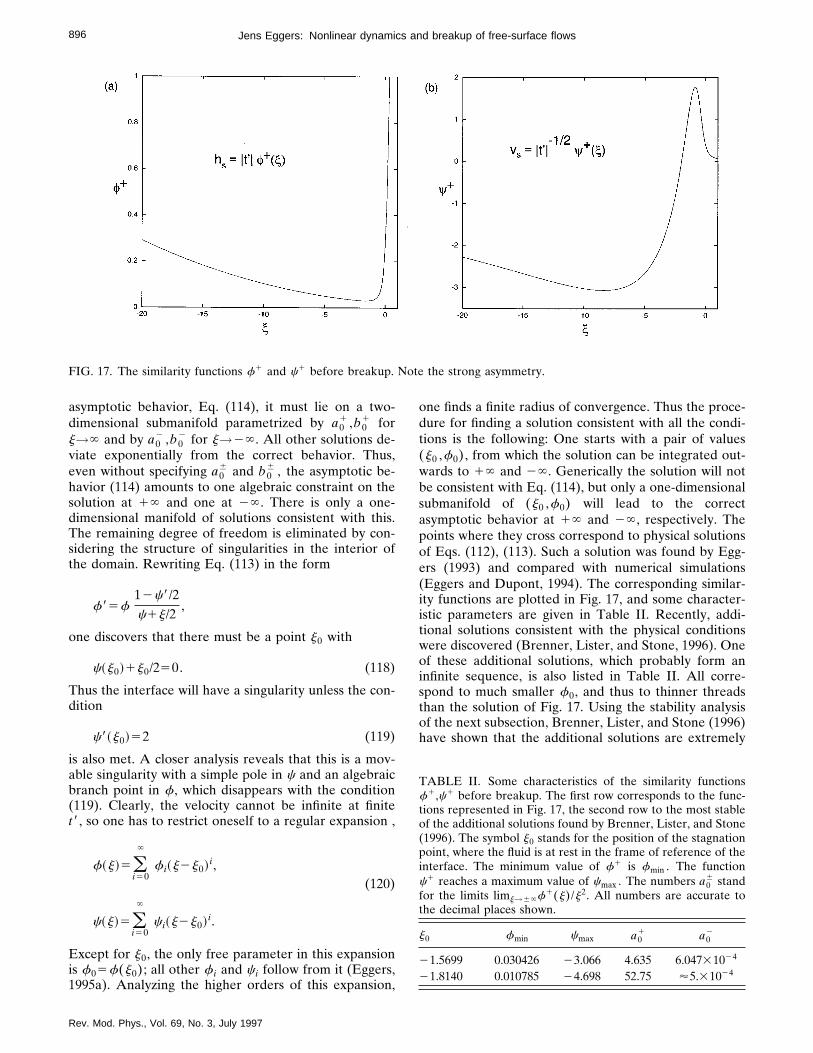
896 Jens Eggers: Nonlinear dynamics and breakup of free-surface flows
FIG. 17. The similarity functions f1 and c1 before breakup. Note the strong asymmetry.
asymptotic behavior, Eq. (114), it must lie on a two-dimensional submanifold parametrized by a0
1 ,b01 for
j→` and by a02 ,b0
2 for j→2` . All other solutions de-viate exponentially from the correct behavior. Thus,even without specifying a0
6 and b06 , the asymptotic be-
havior (114) amounts to one algebraic constraint on thesolution at 1` and one at 2` . There is only a one-dimensional manifold of solutions consistent with this.The remaining degree of freedom is eliminated by con-sidering the structure of singularities in the interior ofthe domain. Rewriting Eq. (113) in the form
f85f12c8/2c1j/2
,
one discovers that there must be a point j0 with
c~j0!1j0/250. (118)
Thus the interface will have a singularity unless the con-dition
c8~j0!52 (119)
is also met. A closer analysis reveals that this is a mov-able singularity with a simple pole in c and an algebraicbranch point in f , which disappears with the condition(119). Clearly, the velocity cannot be infinite at finitet8, so one has to restrict oneself to a regular expansion ,
f~j!5(i50
`
f i~j2j0! i,(120)
c~j!5(i50
`
c i~j2j0! i.
Except for j0, the only free parameter in this expansionis f05f(j0); all other f i and c i follow from it (Eggers,1995a). Analyzing the higher orders of this expansion,
Rev. Mod. Phys., Vol. 69, No. 3, July 1997
one finds a finite radius of convergence. Thus the proce-dure for finding a solution consistent with all the condi-tions is the following: One starts with a pair of values(j0 ,f0), from which the solution can be integrated out-wards to 1` and 2` . Generically the solution will notbe consistent with Eq. (114), but only a one-dimensionalsubmanifold of (j0 ,f0) will lead to the correctasymptotic behavior at 1` and 2` , respectively. Thepoints where they cross correspond to physical solutionsof Eqs. (112), (113). Such a solution was found by Egg-ers (1993) and compared with numerical simulations(Eggers and Dupont, 1994). The corresponding similar-ity functions are plotted in Fig. 17, and some character-istic parameters are given in Table II. Recently, addi-tional solutions consistent with the physical conditionswere discovered (Brenner, Lister, and Stone, 1996). Oneof these additional solutions, which probably form aninfinite sequence, is also listed in Table II. All corre-spond to much smaller f0, and thus to thinner threadsthan the solution of Fig. 17. Using the stability analysisof the next subsection, Brenner, Lister, and Stone (1996)have shown that the additional solutions are extremely
TABLE II. Some characteristics of the similarity functionsf1,c1 before breakup. The first row corresponds to the func-tions represented in Fig. 17, the second row to the most stableof the additional solutions found by Brenner, Lister, and Stone(1996). The symbol j0 stands for the position of the stagnationpoint, where the fluid is at rest in the frame of reference of theinterface. The minimum value of f1 is fmin . The functionc1 reaches a maximum value of cmax . The numbers a0
6 standfor the limits limj→6`f1(j)/j2. All numbers are accurate tothe decimal places shown.
j0 fmin cmax a01 a0
2
21.5699 0.030426 23.066 4.635 6.04731024
21.8140 0.010785 24.698 52.75 '5.31024

897Jens Eggers: Nonlinear dynamics and breakup of free-surface flows
FIG. 18. A sequence of close-ups of a highly viscous jet(l n5274.5 mm, tn5627.9 ms)350 ms, 198 ms, and 46 ms awayfrom breakup. The frame widthcorresponds to 1 mm. The fullline is the prediction of the scal-ing theory of Eq. (111) withscaling function f1 of Fig. 17.Each frame has been cut at topand bottom, so only a smallportion of the drop forming onthe right is seen. The picturesare from the series of experi-ments GLY1 (see Table 1 ofKowalewski, 1996).
unstable, so the only one of physical relevance is the onewith the largest f0, originally found by Eggers (1993).
Note that using this pair of similarity functions, thefull solution near the pinch point can be predicted with-out adjustable parameters. For example, at a given timet02t5tnut8u away from the singularity, the minimum di-ameter of the fluid thread is 0.06l nut8u. So if t02t ismeasured experimentally, the entire profile close to thesingularity can be predicted without adjustable param-eters. This was done in a recent series of jet experimentswith high-viscosity fluids (Kowalewski, 1996).
Figure 18 shows a closeup of the pinch region for a jetconsisting of a mixture of glycerol and alcohol at times350, 198, and 46 ms before breakup, which correspondsto the reduced times ut8u50.56, 0.32, and 0.073. The jetdiameter at the nozzle is 0.397 mm, which is about athird of the image width. When considering the thinthread, one is looking at a part of the solution that ismoving on scales very different from the one set by theundisturbed jet. The experimental pictures have beensuperimposed with the theoretical prediction. Since t8 isknown, there is no adjustable parameter in this compari-son. The theoretical prediction for the position of theminimum is marked by an arrow, which is seen to movetoward the drop adjacent to the thread. In (a), the solu-tion has only started to converge on its left, so there issome discrepancy in the position of the minimum. Astime goes on, the range of validity of the similarity solu-tion expands.
One immediately notices the asymmetry of the solu-tion, which is already apparent from the scaling func-tions (see Fig. 17). The flatness of the neck is much ex-aggerated by the scaling of Eq. (111), which expandsaxial scales relative to the radius. As the slope becomesof order one near the drop, the similarity solution nolonger applies. To extend the prediction beyond therange of validity of the similarity solution, one wouldhave to find an outer solution that described the drop
Rev. Mod. Phys., Vol. 69, No. 3, July 1997
and to match it onto the inner solution. In so doing, onehas to remember that the outer solution will depend onall the experimental details such as the nozzle diameter,the fluid parameters, and the driving mechanism. On theother hand, the pinching solution is independent ofthese details, as confirmed by Kowalewski (1996) whenhe performed experiments with different nozzle diam-eters and fluid viscosities.
However, as the thread becomes thinner, a new andunexpected behavior sets in, shown in Fig. 19 for a fluidof higher viscosity. The interface assumes an irregularappearance with bulges on its surface. Apparently, thesimilarity solution has become unstable in its interior.This instability was first described experimentally by Shi,Brenner, and Nagel (1994), who offered a theoreticalexplanation in Brenner, Shi, and Nagel (1994). Thiswork will be presented in the next subsection.
C. Stability and the influence of noise
It is apparent from Fig. 19 that the similarity solutionis prone to the growth of localized perturbations or‘‘bumps.’’ It seems as if this should be expected from thestability analysis of a liquid cylinder, which the solutionvery much resembles as it is becoming thinner. In fact,it follows from the high-viscosity limits (35) and (36)that the typical wavelength of a bump will belbump;r0(l n /r0)1/4, while the time scale over which itgrows is tbump;tnr0 /l n , so it is localized on the scale ofthe thread length and grows over the same time scale onwhich the solution is evolving. The reason the similaritysolution is still observed is that the flow in the thread hasa stabilizing effect: perturbations are both stretched andconvected out of the pinch region, where they no longergrow. Only perturbations that are sufficiently large ini-tially will affect the similarity solution. This leads to anonlinear instability, quite similar to the fingering insta-

898 Jens Eggers: Nonlinear dynamics and breakup of free-surface flows
bility in Hele-Shaw flow (Bensimon et al., 1986), or den-dritic growth (Kessler et al., 1988).
For an analytical study of the stability problem, suchas was presented by Brenner, Shi, and Nagel (1994), onetakes advantage of the perturbations being localized.Thus it is sufficient to keep track of the center of massand the characteristic width of a localized wave packet.Close to the similarity solution one can work within theframework of the asymptotic equations (79), (80). How-ever, one has to keep some of the higher-order terms inthe mean curvature in Eq. (82), since they are respon-sible for selecting the characteristic size of the bump. Byrewriting the equations in terms of the logarithmic timedistance s5lnut8u from the singularity and the similarityvariable j , one is working on the scale of the similarity
FIG. 19. The same experiment as in Fig. 18, but with a fluid ofhigher viscosity, (l n52 mm, tn512.8 ms, series GLY3 of Kow-alewski, 1996). The height of the frame corresponds to 2 mm.Just before breakup, the thin thread has become unstable andproduced several ‘‘bumps.’’ The moment of breakup showsirregular breakup at several places.
Rev. Mod. Phys., Vol. 69, No. 3, July 1997
solution. This leads to the ansatz
hs~z8,t8!5ut8u(f~j!1f ~j ,s !),(121)
vs~z8,t8!5ut8u21/2(c~j!1c ~j ,s !),
where f(j) and c(j) are the solutions to the similarityequation described in the previous subsection, and f ,c are small perturbations to it. Using a prime to indicatedifferentiation with respect to j , one has the linearizedequations of motion
]sf ~j ,s !5f 2S c1j
2 D f 82f8c 2c8
2f 2
f
2c 8,(122)
]sc ~j ,s !52c
22S c1
j
2 D c 82c8c 1f 8
f2 22f8
f3f
13c 916f8
fc 816
c8
ff 826
c8f8
f2 f 1t8f -.
From the higher-order terms of the mean curvature wehave included only the highest derivative of the pertur-bation, since it is the one which limits the wavelengthfrom below.
Solutions of the linear problem (122) have the form
S f
c D 5S cosq
sinq D exp$S~z ,j ,s !%, (123)
where the exponential describes the growth of perturba-tions. By having S depend on j and z5j/e , one sepa-rates the short-wavelength perturbation, which moveson the scale of z , from the slowly varying ‘‘background’’of the similarity solution. The ansatz
S~z ,j ,s !51e
b0(k~s !,j)s1ik~s !z1b1(k~s !,j)s (124)
describes a perturbation of wavelength e/k(s), which isconvected with velocity b0 /k(s) in similarity variables,and whose amplitude grows with rate b1. Indeed, plug-ging Eqs. (123), (124) into the linearized equations, onefind to leading order e21
b052ik~s !~c1j/2! (125)
and
]sk52k~s !S c8112 D . (126)
This means a bump is convected with the interfacial ve-locity
c i5c1j/2,
which is the velocity of the fluid in the frame of refer-ence of the surface. At the stagnation point j0 [see Eq.(118)], the bump always remains on the same point ofthe surface. At the same time, the bump is stretchedwith rate 2(c811/2), which is negative in the neck re-gion (see Fig. 17). Hence the wavelength increases, mak-ing the disturbance more benign.
The temporal growth rate is

899Jens Eggers: Nonlinear dynamics and breakup of free-surface flows
FIG. 20. A photograph of a glycerol in water mixture (85 w%) (Shi, Brenner, and Nagel, 1994). Part (a) is an overall view showinga tiny microthread growing out of the initial neck, (b) is a magnified view of the ‘‘micro-thread,’’ which is close to a similaritysolution 231023 s away from breakup. Image (c) shows the same neck as in (b), but at a later time. One observes an even smallerneck growing out of the original micro-thread, which is again a similarity solution with the estimated breakup time of 231024 s.Reprinted with permission. © American Association for the Advancement of Science.
b1~k ,j!511c8
21
16fF12t8S f
k
e D 2G (127)
which can be translated into a spatial growth rate byc i ,
]jA
A~j!5
b1
c i, (128)
where A(j) is the amplitude of a bump at j . IfA05A( j ) is the initial amplitude at a reference pointj , Eq. (128) can be solved to give
A~j!
A05expH E
j
jb1~j8!
c i~j8!dj8J . (129)
From this it seems as if arbitrary growth could be ob-tained for j 5j0, leaving a bump at the same point for-ever. But that would require an arbitrarily sharp spike,while a bump with positive growth rate must have ap-proximate size t81/2 according to Eq. (127). Thusj 't81/2 should be taken as the lower limit in Eq. (129).On the other hand, an analysis of Eq. (129) for largeuju reveals, using f5a0
6j2 and c5b06j21, that a bump
no longer grows for j→6` . Such a bump, which is fro-zen in on the time scale of the singularity, has beencalled a ‘‘blob.’’ When one uses the parameters of thesimilarity solution, any bump that gets convected toj2'210 or j1'1.5 meets such a fate.
This completes the input necessary to estimate the
Rev. Mod. Phys., Vol. 69, No. 3, July 1997
critical amplitude that makes the similarity solution un-stable. The amplitude A(j) has to grow to the same sizeas the similarity solution itself before it reaches j2 orj1 , starting from j 't81/2. Using this condition, Brenner,Shi, and Nagel (1994) estimated the critical amplitudefor surface perturbations to be
Ac5231025t81.495 (130)
in units of the minimum thickness. In real space thismeans that for a thread of radius h0 one needs a surfaceperturbation of size
hc53.831023h0S h0
l nD 1.495
(131)
to render the interface unstable. Thus in the late stagesof singularity formation, for which h0!l n , the solutionbecomes more and more vulnerable to external pertur-bations, in qualitative agreement with experiment. Fig-ure 20 shows a picture of a mixture of glycerol and waterfalling from a nozzle. Part (b) is a magnification of thethin thread in (a), which is close to the similarity solu-tion, 2 ms away from breakup. In part (c) this solutionhas undergone an instability, and a smaller neck hasgrown on it, which is again well approximated by a simi-larity solution, 200 ms away from breakup.
This conclusion is amplified by a series of numericalsimulations of the asymptotic model (79), (80), and (82)with some stochastic noise added to it. Figure 21 shows a

900 Jens Eggers: Nonlinear dynamics and breakup of free-surface flows
simulation with the same parameters as in the experi-ment (see Fig. 20). The first picture (a) shows the samethread as was in the experimental picture. Withoutnoise, it evolves according to the similarity solution upto breakup. However, once noise is added, one observes[see Fig. 21(b)] tiny necks growing on the original simi-larity solution, similar to Fig. 20(c). In the simulationone can follow up on this solution, and observe still an-other neck growing on that of the previous stage. Inter-estingly, one confirms that each of those necks repre-sents another similarity solution, but with a differentvalue of z0 and t0. If numerical resolution is increased,this cascade of similarity solutions can be followedthrough an arbitrary number of instabilities, Fig. 21(c),going down to the stage of the seventh neck. The abovestability analysis has been repeated by Brenner, Lister,and Stone (1996) for the additional similarity solutionsfound by them, one of which is listed in Table II. Forthese solutions, the analogue of the critical amplitude(130) is much smaller, so they immediately go unstableand converge to the similarity solution described above,even if care is taken to reduce the noise as much aspossible.
The main open problem is the source of the noise thatcauses the instability. A possibility discussed by Bren-ner, Shi, and Nagel (1994) is thermal capillary waves,whose amplitude can be estimated using the theory ofhydrodynamic fluctuations (Landau and Lifshitz, 1984a).The result is that thermal fluctuations become importantwhen the minimum radius becomes of the order of
h thres55l nS l T
l nD 0.401
, (132)
where
l T5~kBT/g!1/2
is the thermal length scale. For the fluid of Fig. 20, this
FIG. 21. Simulation of a drop of viscous fluid for the samephysical parameters as in Fig. 20 (Shi, Brenner, and Nagel,1994). The left frame (a) shows the same view as in Fig. 20(a),while (b) is an enlargement of the micro-thread region, simu-lated in the presence of noise. In addition to the neck seen inFig. 20(c), which has grown out of the original micro-thread,one sees another stage of the sequence of instabilities. Part (c)suggests that this sequence of instabilities goes on indefinitely,by showing further enlargements of the unstable region.
Rev. Mod. Phys., Vol. 69, No. 3, July 1997
gives h thres51 mm, which rather underestimates thescale where irregular behavior is observed in experi-ment. On the other hand, in the jet experiment of Fig. 18one finds h thres510 mm, while the smallest radius in Fig.18 is about 1 mm. Clearly, more carefully controlled ex-periments are needed to quantitatively identify possiblesources of the noise.
Finally, we mention that a comparison with the stabil-ity analysis of Sec. IV.A implies that the axisymmetricsingularity will be stable against nonaxisymmetric distur-bances. Strictly speaking, the singularity could still benonaxisymmetric if the initial condition deviates greatlyfrom axisymmetry. On the other hand, a spherical crosssection corresponds to a global minimum in surfacearea, with oscillations strongly damped by viscosity, so itis hard to see how nonaxisymmetry could persist. An-other possible departure from the proposed universalsolution could lie in a nonzero azimuthal velocity field,driven through the nonlinear coupling of the Navier-Stokes equation. Both possibilities are worthwhile sub-jects of theoretical and experimental research.
D. After breakup
Having investigated the structure of solutions up tothe point of breakup, one finds it natural to ask what thebehavior will be after breakup. At a scale l micro the in-terface will be broken by some microscopic mechanism,whose nature cannot be investigated within the frame-work of hydrodynamics. One possible guess is that thisscale is on the order of intermolecular distances. In themolecular dynamics calculations of Koplik and Banavar(1993), pinching of threads ten molecules in diameterwas observed. Although the behavior was reminiscent ofhydrodynamic behavior, no quantitative comparison wasattempted, so the questions of mechanisms of ruptureand up to what scale to apply hydrodynamics are reallyopen in the case of free surfaces. At high viscosities, theinstability described in the previous subsection willmake the interface look ‘‘fuzzy’’ and ever more suscep-tible to (multiple) breakings. The scale at which a dropbreaks can expected to be much larger than moleculardistances if the viscosity is large. Whatever the scale maybe, the fundamental problem is whether the subsequentevolution depends on the microscopic aspects of thebreaking on scales much larger than l micro . If it is inde-pendent, the mathematical equivalent is that there is aunique prescription to continue the equations of motionbeyond the singularity.
Questions of this type have been investigated exten-sively on a mathematical level (Altschuler, Angenent,and Giga, 1995). This was done mostly for geometricalevolution problems like that of mean curvature flow(Huisken, 1991; Deckelnick, 1997), but also for the non-linear Schrodinger equation (Giga and Kohn, 1989;Merle, 1992), for which the continuation is not unique.The reason is that the complex wave function can pickup an arbitrary phase after breakup. The problem of aliquid bridge is very different because it includes inertia.This prevents fluid away from the breakup point from

901Jens Eggers: Nonlinear dynamics and breakup of free-surface flows
moving much on the time scale of the breaking, whichindicates that the solution (now consisting of two parts)should indeed be independent of the mechanisms ofbreakup. The most direct way to show this is, of course,to construct explicitly a solution in a similar vein to thatin which similarity solutions were found before breakup.Similarity solutions that correspond to a unique continu-ation through a singular point in time were constructedfor the porous-medium equation by Grundy (1983), andfor the shallow-water equations by Grundy and Bell(1993). Keller and Miksis (1983) have constructed simi-larity solutions of an inviscid wedge of fluid afterbreakup. The asymptotics far away from the point ofbreakup enter the solution as a free parameter. In ourcase the asymptotic behavior is already known: it shouldcoincide with the solution before breakup, so the param-eters are uniquely determined.
Figure 22 shows a schematic view of a receding neckafter breakup. The same asymptotic equations as beforebreakup apply, since shortly after breakup the solutionwill still be a thin thread. However, the situation is dif-ferent in the immediate neighborhood of the tip, whereh8 diverges and thus renders Eqs. (79) and (80) inappli-cable. In fact, as h→0 and h8→` near the tip, both theviscous term (h2v8)8/h2 and the asymptotic form of thepressure gradient 2h8/h2 diverge. Thus one is facedwith a boundary-layer problem: the thin tip region obeysa different type of scaling than the outer region, andtherefore other equations apply. Both inner and outersolutions have to be accommodated by matching condi-tions. To establish the proper scaling, one observes thatin the frame of reference of the receding tip the end isalmost static, so it will approach a spherical equilibriumshape on a microscopic time scale. This means the sizeof the tip region l tip is the same as its radial extension.Since the tip has to be matched onto the outer solution,both radial scales must coincide, and we havel tip'l nut8u, using the scaling of the outer solution. Thismeans that in the scaling limit t8→0 the size of the tip
FIG. 22. A cartoon of a receding tip after breakup. The size ofthe tip region l tip is the same as the typical width of the neck.
Rev. Mod. Phys., Vol. 69, No. 3, July 1997
region goes to zero even in similarity variables. Hencethe similarity equations (112), (113) can be applied up tothe position of the tip
j tip5ztip8 ut8u1/2
in the limit t8→0.In his early study of inviscid receding threads Keller
(1983) went beyond this asymptotic limit. There and inthe somewhat more explicit treatment by Keller, King,and Ting (1995) both parts of the solution were consid-ered, which scale differently. Using mass and momen-tum balances, as well as matching conditions, approxi-mate solutions for the tip region and the neck werefound. By contrast, Eggers (1995a), using the full viscoustheory, considered only the limit t8→0 in which the tipregion shrinks to zero. In that case, a unique answer forthe shape of the neck was obtained. The only propertyof the tip solution needed was that all terms of the equa-tion remain finite as one approached the tip, the under-lying assumption being that the exact form of the tipsolution does not matter.
The idea behind the solution proposed by Eggers(1995a) was to supplement the asymptotic equations(79)–(81) with higher-order terms, which remove thesingularity at the tip. The solution of the regularizedequations is thus valid at the tip and can be analyzed inthe limit ut8u→0. This leads to a unique answer for theasymptotic form of the tip, independent of the regular-ization chosen. To produce a regular tip, one can gener-alize the equations to the form (Constantin, 1992)
] th1vh852v8h
2, (133)
] tv1vv852p8/r1~v8D2!8
h2 , (134)
where
p51
2hF]E
]h2S ]E
]h8D 8G .
Here E(h ,h8) is a surface energy and D(h ,h8) a dissi-pation kernel. Equation (134) can also be rewritten inthe form
] tv1vv851h2 @2G/r1v8D2# ,8 (135)
where
G~h ,h8!5h2p1h8]E
]h82E . (136)
From this one immediately derives the energy conserva-tion equation
] t@h2v2/21E~h ,h8!#52~v8D !21boundary terms,
which motivates the nomenclature for E and D . As faras the asymptotic analysis is concerned, the only infor-mation needed from G and D appearing in Eq. (135) isthat they vanish at the tip. This is a direct consequence

902 Jens Eggers: Nonlinear dynamics and breakup of free-surface flows
FIG. 23. The similarity functions f2 and c2. The asymptotic behavior for j→6` is the same as before breakup. On the left sideis the rapidly receding ‘‘neck’’ part of the solution, on the other side is the drop. The points jneck and jdrop , from where theinterface is plane, are marked by diamonds.
)
)
)
)
)
of the pressure gradient and the dissipation term’s beingfinite near a regular tip h;(z2z tip)1/2.
The equations of motion (133) and (135) need only beanalyzed in a small region of size l tip , where the fluidhas to move with the receding tip. Therefore, in coordi-nates moving with the tip position, the inertial termsdrop out. In terms of similarity variables, the transfor-mation to the comoving frame reads
f ~ j !5f~j 1j tip!,
c ~ j !5c~j 1j tip!2j tip/2, (137
j 5j2j tip .
Plugging the similarity ansatz (111) into the equations ofmotion, one finds the similarity equations
f 52c 8f /2, (138
@2G 1c 8D 2#850 (139
in the tip region of size j 'ut8u1/2. As remarked above,G and D are zero at the tip, so Eq. (139) can actually bewritten
G 5c 8D 2. (140
At j 'ut8u1/2, the asymptotic form of the equations be-come valid, and comparing Eqs. (139) and (112) we canwrite
G asymp52f , D asymp5A3f . (141
Thus from Eqs. (138), (140), and (141) one finds thatf 51/6, so the correct boundary condition for f at thetip is
f~j tip!51/6. (142)
Now we can solve the similarity equations (112), (113)
Rev. Mod. Phys., Vol. 69, No. 3, July 1997
with the boundary condition (142). Note that after thesingularity the minus sign applies. The solution near thetip has the expansion
f51/61f1~j2j tip!2/51••• , (143)
c5j tip/222~j2j tip!1e0~j2j tip!7/51••• .
All the coefficients can be calculated from the two pa-rameters f1 and j tip , which still need to be determined.Because of the change of sign in the equations, one nowhas exponential convergence onto the solutions with theasymptotics (114), as one integrates outwards toj→6` . The constants a0, b0 are open and depend onf1, j tip . The solution is thus uniquely fixed by requiringthat the constants a0 ,b0 before and after the singularitycoincide. This is because the solution far outside the sin-gularity is unaffected by the breaking. The resultingsimilarity functions are plotted in Fig. 23, while some ofthe characteristic parameters are given in Table III. Thesolution now consists of two parts, one representing areceding thread, the other just a small perturbation of adrop. Although obtained by the same procedure, theylook very different, as the constants a0 and b0 are verydifferent to the left and right of the singularity.
Figure 24 shows a particular example of how the so-lution before breakup is uniquely continued. After
TABLE III. Characteristics of the similarity functions f2,c2
after breakup. The tip position of the left-hand, or neck side isjneck , and the expansion coefficient f1 [cf. Eq. (143)], isfneck . Correspondingly, jdrop and fdrop uniquely determine the‘‘drop’’ side of f2 and c2. The values of a0
6 and b06 are the
same as before breakup (see Table II).
jneck fneck jdrop fdrop
17.452 0.06183 0.4476 0.6180

903Jens Eggers: Nonlinear dynamics and breakup of free-surface flows
breakup, one part of the solution consists of a rapidlyreceding thread, the position of the tip being
z tip2z05l njneckt81/2.
Thus the tip velocity goes like ut8u21/2, making it sloweras t8 gets larger. The other part of the solution is visibleas a small protuberance, which rapidly heals off to analmost flat interface.
Detailed comparisons of the similarity solution afterbreakup with numerical simulations of Eqs. (133) and(134) are reported in Eggers (1995a). This is docu-mented in Fig. 25, which shows the approach of the simi-larity solution by a sequence of profiles calculated fromEqs. (133), (134), immediately after the interface hadbeen cut. It was verified in (Eggers, 1995a) that this simi-larity solution is independent of the particular regular-ization used in Eq. (133). Thus the continuation indeedturns out to be unique, independent of the detail of thedynamics near the tip.
As far as comparison with experiment is concerned,the situation is less fortunate. Figure 26 shows the con-tinuation of the series of pictures presented in Fig. 18.Qualitatively, the solution looks as predicted. But whilethe comparison with similarity theory is fully quantita-tive before breakup, two problems arise after breakup:First, there is some residue left between the two parts ofthe solution, which is seen as two tiny drops. This isbecause there is some unsteadiness in the solution be-fore breakup, as can be seen in Fig. 26(a), which makesthe thread break in more than one place. Second, theretraction speed is slower than is predicted by theory. InFig. 26(b) we have estimated the time distance from
FIG. 24. The breakup of a mixture of glycerol in four parts ofethanol, as calculated from the similarity solutions. Part (a)shows three profiles before breakup, in time distances of 46ms, corresponding to ut8u51, 0.55, and 0.1. In part (b) the sameis shown after breakup.
Rev. Mod. Phys., Vol. 69, No. 3, July 1997
breakup to be 6.7 ms, based on the position of the tipaccording to the similarity theory. The drop part of thesolution is well represented by the similarity solution,while at the end of the thread some additional fluid hasaccumulated, probably a result of blobs formed in theirregular breakup. The distance the tip has retracted inFig. 26(c) is only 80% of that predicted by theory on thebasis of the timing of Fig. 26(b). The reason is probablythe air drag on the tiny thread, which according to thesimilarity solution should have a speed of 37 m/s and athickness of 0.6 mm in Fig. 26(b). While slender-bodytheory predicts the force due to air drag to be almostindependent of the thread radius (Happel and Brenner,1983), the force of retraction diminishes with the crosssection. Thus the thread is very sensitive at small diam-eters. Close to breakup one therefore expects the tip tospeed up rather than to slow down. Examples of thisbehavior have been observed by Kowalewski (1996), us-ing the ‘‘frame-transfer’’ technique. Observations inqualitative agreement with Kowalewski’s have also beenmade by Henderson, Pritchard, and Smolka (1997). Tobe able to make a quantitative comparison one mustconsider two possible approaches: The first is to includethe outer fluid. Such a theory is being developed byLister and Stone (1996). The other approach is to reducethe air drag as much as possible in order to observedirectly the similarity solution. Some experiments in thisdirection were performed by Kowalewski (1996) in anevacuated chamber, using an oil of high vapor pressure.However, a comparison with theory is difficult since thebreakup was quite unsteady in this particular series ofexperiments. It would be preferable to work with fluids
FIG. 25. The approach of the similarity function f2 by thesolution of Eqs. (133) and (134) in the jet geometry, trans-formed to similarity variables. The fluid neck is severed atut8u51024 before breakup. The full line is f2, the dotted linethe solution before breakup. The dot-dashed and the dashedlines show the simulation at ut8u50.006 and ut8u50.06, respec-tively.

904 Jens Eggers: Nonlinear dynamics and breakup of free-surface flows
FIG. 26. Continuation of thesequence of Fig. 18, 6.7 ms be-fore breakup, as well as 6.7 msand 22 ms after breakup. Thefull line is the prediction of thesimilarity theory. The timing of(b) was estimated on the basisof this solution.
of somewhat lower viscosity, making the solution lesssensitive to noise.
VII. AWAY FROM BREAKUP
A. High viscosity—threads
A familiar feature of the breakup of high-viscosity liq-uids is their tendency to produce very long and thinthreads. As seen in the previous section, threads alwaysoccur in the last stages of pinching. But the most dra-matic effects occur when the Reynolds number is al-ready small, based on the initial extension and velocityof the fluid, and when threads are drawn by some exter-nal pull. This way, mm diameter threads can easily beextended to the length of several cm. This is known notonly from breakfast table experiments, but also from im-portant industrial processes like fiber spinning. An ex-ample is shown in Fig. 27, in which gravitational pull isresponsible for producing a thread of glycerol approxi-mately 2 cm long.
According to Rayleigh’s theory, the time scale onwhich disturbances grow increases with viscosity, butthis can by no means account for the persistence ofthreads at such small diameters. In fact, the time scaleover which a thread should become unstable istn5r0rn/g . Even for a fluid of such high viscosity asglycerol, but with a thread radius of 10 mm, the timescale is tn5230 ms, which is much shorter than the timeover which the thread is pulled out in Fig. 27. So, clearly,the flow inside the thread has to be taken into account,just as it was in the stability analysis of the Sec. VI.C. Sofar, a quantitative explanation for the stability of threadsin these more general circumstances has not been of-fered. Pearson and Matovich (1969) looked at the stabil-ity of an extending liquid thread, but did not includesurface tension, which is the source of the potentially
Rev. Mod. Phys., Vol. 69, No. 3, July 1997
most dangerous instability. By analogy to the analysis ofthe previous section, both convection and a positivestretching rate will be important. Disturbances are con-vected out of regions where the thread is thinnest, andstretching pulls disturbances apart, lowering their ampli-tude. Most likely, the conditions under which a thread isstable are much more general than the specific case of asimilarity solution. This remains an extremely interest-ing problem to be studied in more detail.
FIG. 27. A drop of glycerol falling from a nozzle 1.5 mm indiameter, pulling out a very long thread (Shi, Brenner, andNagel, 1994). Reprinted with permission. © American Asso-ciation for the Advancement of Science.
905Jens Eggers: Nonlinear dynamics and breakup of free-surface flows
Even without gravitational pull, threads can extend tothe size of the external scale if the Reynolds number issufficiently small. Evidence is provided by the picturesof jets and liquid bridges at high viscosities (see Figs. 5and 8). Here it is surface tension itself that pulls out thethreads and collects all the fluid in drops. The length ofthe thread is set by the wavelength of the perturbationand, as we shall see below, it thins almost uniformly ifthe Reynolds number is sufficiently low. We shall con-centrate on this case for our discussion of threads, sincerecently a new type of similarity solution has been foundthat describes the thinning of jets at very high viscosities(Papageorgiou, 1995). If the Reynolds number is smallinitially, the evolution is governed by the Stokes equa-tion (16). Going through the same thin filament analysisas was developed for the case of the Navier–Stokesequation, one effectively drops the inertial terms] tv1vv8 in the lubrication equation for the axial veloc-ity (79). Since surface tension and viscous forces are nowthe only forces to be balanced, there is additional scalingfreedom in the equations. As a result, singular solutionscan have the form
hs~z8,t8!5ut8ufSt~j!,
vs~z8,t8!5ut8ub21cSt~j!, (144)
j5z8/ut8ub,
where the exponent b is to be determined. The scaling(111) is recovered for b51/2. Although Eq. (144) sug-gests the existence of a solution for any b , a particularb is selected by the dynamics, as Papageorgiou showed.The value is close to b50.175, which means that theaxial scale of this solution contracts at a much slowerrate than it does for the asymptotic solution (111). Plug-ging Eq. (144) into the full equations (79), one finds thatthe surface tension and the viscous terms scale likeut8u212b'ut8u21.18, while the inertial terms are propor-tional to ut8u221b'ut8u21.83. This means that in the sin-gular limit the terms neglected in the Stokes approxima-tion become larger than those retained. Hence, fort8→0 the Stokes solution is no longer consistent butmust give way to the asymptotic solution, in which allforces are balanced. Note that Papageorgiou (1995)makes an erroneous statement to the contrary.
To derive the Stokes solution, we shall use a presen-tation somewhat different from Papageorgiou’s, usingthe Lagrangian description of Sec. V.D. This allows oneto do almost all calculations analytically. Dropping theinertial term ztt from Eq. (96), one finds
05g
r~za
21/2!a13nS zta
za2 D
a
, (145)
which can be integrated to give
C~ t !5g
rH26nHtH , (146)
where H(a ,t)5za21/2(a ,t) is the height of the interface
in Lagrangian coordinates and C(t) is independent ofa . This description was first given by Renardy (1994).
Rev. Mod. Phys., Vol. 69, No. 3, July 1997
What is remarkable about Eq. (146) is that all spatialderivatives have dropped out. Hence spatial informa-tion, for example the characteristic width of the modu-lation, can only enter through the initial conditions.
We now look for the singular contribution to H , rela-tive to the singular point a0 ,t0, in units of l n ,tn :
H~a ,t !5l nHs~a8,t8!,
a85~a2a0!/l n3 , (147)
t85~ t02t !/tn .
Then the self-similar ansatz equivalent to Eq. (144) is
Hs~a8,t8!5ut8ux~z!,(148)
z5a8/ut8u21b.
Plugging this into the equations of motion (146), onefinds the similarity equation
C 5x16x226~21b!zx8x , (149)
where C is a constant. Remembering thatH22(a ,t)5za(a ,t), and therefore x225Fz for a suit-able F , one finds that
C 5
E2`
`
x23~z!dz
E2`
`
x24~z!dz
. (150)
Thus the additional constraint (150) is a direct conse-quence of volume conservation, as expressed by Eq.(93). Equations (149) and (150) can be used to computethe constants C and b . First, Eq. (149) can be integratedto give
lnU z
z0U56~21b!E
x0
x z8dz8
6z821z82C. (151)
From the symmetry of the similarity equations one con-cludes that x(z) is symmetric and takes its minimum atz050: x05x(0). The expansion of x around the mini-mum looks like
x~z!5x01z21x4z41••• , (152)
where the quadratic coefficient was normalized to one.By demanding that the singularities in Eq. (151) cancelas z0→0, one finds that
x051
12~11b!, (153)
C 5312b
24~11b!2 . (154)
When one does the integral in Eq. (151), the explicitexpression for the inverse of x is
z5S 6~11b!
21b D ~312b!/2Fx1312b
12~11b!G~312b!/2
3~x2x0!1/2. (155)
Now Eq. (150) can be used to derive an eigenvalue re-lation for b , using the transformation dz5x821dx :

906 Jens Eggers: Nonlinear dynamics and breakup of free-surface flows
FIG. 28. Scaling functions of the Stokes similarity solution, fSt and cSt .
` a
)
312b
24~11b!2 5
Ex0
~dx/x8x3!
Ex0
`
~dx/x8x4!
.
Employing both Eqs. (149) and (155), the integrals leadto hypergeometric functions F , so one finally has (Grad-shteyn and Ryzhik, 1980)
~12b!~312b!
~11b!~322b!5
F~21/22b ,12b ,3/22b ,2322b!
F~21/22b ,22b ,5/22b ,2322b!,
(156)
which is the desired equation for b . Incidentally, theparticular ratio of hypergeometric functions appearingin Eq. (156) can be evaluated very efficiently in acontinued-fraction representation (Bender and Orszag,1978, p. 396), giving
b50.17487 . . . , (157)
in agreement with Papageorgiou’s result. Brenner,Lister, and Stone (1996) have shown that the solutionthus found is not the only one, but again there is aninfinite sequence of solutions. They correspond to thefirst nonvanishing term in the expansion of x being notof second order, as in Eq. (152), but of higher-order.Again, the higher order solutions are much more un-stable than the one corresponding to Eq. (157). But thisis not all. By a combination of asymptotic analysis andnumerics, Renardy (1995) has shown that singularitieswith power laws different from (144) may occur, de-pending on initial conditions. In particular, the exponentwith which the local radius goes to zero as a function ofut8u may vary continuously between 1/2 and the value 1of Eq. (144). In the case of slowly varying initial data,however, the present Stokes solution is expected to oc-cur.
Finally, to transform back from Lagrangian coordi-nates to real space, one has to integrate the relation
Rev. Mod. Phys., Vol. 69, No. 3, July 1997
z85E0
H22~ a ,t !da .
In similarity variables, this amounts to
j
j5E
1
fSt~j!/x0 ~x1312b!~112b!/2
x~x21 !1/2 dx , (158)
where the integral can be done numerically withoutgreat fuss. The normalization length j is arbitrary anddepends on initial conditions. For practical purposes onewill have to fit it to experiment. Both scaling functionsfSt and cSt in the Stokes case are plotted in Fig. 28. Thescaling function cSt of the velocity is found from
cSt~j!5E0
j 6x021x02fSt~ j !
3fSt2 ~ j !
d j . (159
A straightforward analysis of the asymptotics for largeuju reveals that
fSt~j!;uju1/b,(160)
cSt~j!;uju~b21 !/b,
as is required for a proper matching onto a static outersolution.
Figure 29 shows the middle portion of the neckbetween two drops in a jet experiment at high viscosity,Re=0.32 (Kowalewski, 1996). As required by the simi-larity solution of the Stokes equation, the solution issymmetric, with the singular point in the middle. In Fig.29(a) we have fitted a similarity solution (144) withut8u50.22 to the neck by adjusting the axial scale. Theminimum thickness of the neck, by contrast, is predictedwithout adjustable parameters and agrees well with ex-periment. This thickness has more than twice the valueone would have expected from the asymptotic similaritysolution, which includes inertia. Part (b) of Fig. 29 showsthe same neck at a later stage, ut8u50.12, compared with
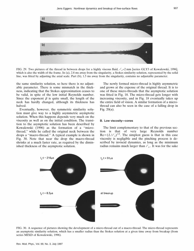
907Jens Eggers: Nonlinear dynamics and breakup of free-surface flows
FIG. 29. Two pictures of the thread in between drops for a highly viscous fluid, l n=2 mm [series GLY3 of Kowalewski, 1996],which is also the width of the frame. In (a), 2.8 ms away from the singularity, a Stokes similarity solution, represented by the solidline, was fitted by adjusting the axial scale. Part (b), 1.5 ms away from the singularity, contains no adjustable parameter.
the same similarity solution, so here there is no adjust-able parameter. There is some mismatch in the thick-ness, indicating that the Stokes approximation ceases tobe valid, in spite of the low initial Reynolds number.Since the exponent b is quite small, the length of theneck has hardly changed, although its thickness hashalved.
Eventually, however, the symmetric similarity solu-tion must give way to a highly asymmetric asymptoticsolution. When this happens depends very much on theviscosity as well as on the initial condition. The transi-tion to the asymptotic solution has been described byKowalewski (1996) as the formation of a ‘‘micro-thread,’’ while he called the original neck between thedrops a ‘‘macro-thread.’’ A typical example is shown inFig. 30. Note that near the drop the macro-threadshrinks at a much faster rate, as required by the dimin-ished thickness of the asymptotic solution.
Rev. Mod. Phys., Vol. 69, No. 3, July 1997
The newly formed micro-thread is highly asymmetricand grows at the expense of the original thread. It is toone of these micro-threads that the asymptotic solutionwas fitted in Fig. 18. The micro-thread gets longer withincreasing viscosity, and in Fig. 18 eventually takes upthe entire field of vision. A similar formation of a micro-thread can also be seen in the case of a falling drop inFig. 20(a).
B. Low viscosity—cones
The limit complementary to that of the previous sec-tion is that of very large Reynolds numberRe5(L/l n)1/2. The simplest guess is that in this caseviscosity is negligible and the pinching process is de-scribed by inviscid dynamics, as long as the minimumradius remains much larger than l n . It was for the sake
FIG. 30. A sequence of pictures showing the development of a micro-thread out of a macro-thread. The micro-thread representsan asymptotic similarity solution, which has a smaller radius than the Stokes solution at a given time away from breakup (fromseries MIXD of Kowalewski, 1996).
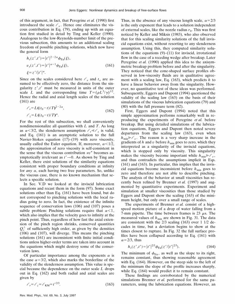
908 Jens Eggers: Nonlinear dynamics and breakup of free-surface flows
of this argument, in fact, that Peregrine et al. (1990) firstintroduced the scale l n . Hence one eliminates the vis-cous contribution in Eq. (79), ending up with an equa-tion first studied in detail by Ting and Keller (1990).Analogous to the low-Reynolds-number limit of the pre-vious subsection, this amounts to an additional scalingfreedom of possible pinching solutions, which now havethe general form
hs~z8,t8!5ut8u222afEu~j!,
vs~z8,t8!5ut8ua21cEu~j!, (161)
j5z8/ut8ua.
Since on the scales considered here l n and tn are as-sumed to be effectively zero, the distance from the sin-gularity z8,t8 must be measured in units of the outerscale L and the corresponding time T5(rL3/g)1/2.Hence the radial and axial length scales of the solution(161) are
l r5L(~ t02t !/T)222a,(162)
l z5L(~ t02t !/T)a.
For the rest of this subsection, we shall convenientlynondimensionalize all quantities with L and T . As longas a,3/2, the slenderness assumption l r!l z is valid,and Eq. (161) is an asymptotic solution to the fullNavier-Stokes equation (17)–(19) with zero viscosity,usually called the Euler equation. If, moreover, a,1/2,the approximation of zero viscosity is self-consistent inthe sense that the viscous contribution nv9 becomes as-ymptotically irrelevant as t8→0. As shown by Ting andKeller, there exist solutions of the similarity equationsconsistent with proper boundary conditions at infinityfor any a , each having two free parameters. So, unlikethe viscous case, there is no known mechanism that se-lects a specific solution.
In Sec. V.D we looked at the inviscid lubricationequations and recast them in the form (97). Some exactsolutions other than Eq. (161) have been found, but donot correspond to pinching solutions with the local ra-dius going to zero. In fact, the existence of the infinitesequence of conservation laws (106) and (107) poses asubtle problem: Pinching solutions require that a,1,which also implies that the velocity goes to infinity at thepinch point. Thus, regardless of how fast the axial exten-sion of the pinch region shrinks, conserved quantitiesQi
6 of sufficiently high order, as given by the densities(106) and (107), will diverge. This means the pinchingsolutions (161) are inconsistent with finite initial condi-tions unless higher-order terms are taken into account inthe equations which might destroy some of the conser-vation laws.
Of particular importance among the exponents a isthe case a53/2, which also marks the borderline of thevalidity of the slenderness assumption. This value is spe-cial because the dependence on the outer scale L dropsout in Eq. (162) and both radial and axial scales aregiven by
l r5l z5l KM5t82/3. (163)
Rev. Mod. Phys., Vol. 69, No. 3, July 1997
Thus, in the absence of any viscous length scale, a52/3is the only exponent that leads to a solution independentof external scales, like the nozzle radius r0. This was firstnoticed by Keller and Miksis (1983), who also observedthat for this scaling similarity solutions of the full invis-cid equations exist, without resorting to any slendernessassumption. Using this, they computed similarity solu-tions of the equations (9)–(11) for inviscid, irrotationalflow in the case of a receding wedge after breakup. LaterPeregrine et al. (1990) applied this idea to the axisym-metric breakup problem before and after the singularity.They noticed that the cone-shaped surface profiles ob-served in low-viscosity fluids are in qualitative agree-ment with a scaling law, Eq. (163), which predicts h tohave a linear behavior away from the singularity. How-ever, no quantitative test of these ideas was performed.Subsequently, Eggers and Dupont (1994) questioned thevalidity of the scaling law (163) on the basis of theirsimulations of the viscous lubrication equations (79) and(80) with the full pressure term (82).
First, Eggers and Dupont (1994) noted that thissimple approximation performs remarkably well in re-producing the experiments of Peregrine et al. beforebreakup. But using detailed simulations of the lubrica-tion equations, Eggers and Dupont then noted severedepartures from the scaling law (163), even whenhmin@l n . The reason is a very sharp increase in thegradients of h and v before hmin goes to zero, which theyinterpreted as a singularity of the inviscid equations,which is stopped only by viscosity. This singularitymakes the viscosity become important while hmin@l n ,and thus contradicts the assumptions implicit in Eqs.(161) and (163). In particular, this implies that the invis-cid equations become inconsistent before hmin goes tozero and therefore are not able to describe pinching.The analysis of the behavior at small viscosities has re-cently been refined by Brenner et al. (1997) and aug-mented by quantitative experiments. Experiment andsimulation at smaller viscosities than those studied byEggers and Dupont show the scaling (163) of the mini-mum height, but only over a small range of scales.
The experiments of Brenner et al. consist of a high-speed motion picture of a drop of water falling from a7-mm pipette. The time between frames is 23 ms. Themeasured values of hmin are shown in Fig. 31. The dataare consistent with the 2/3 scaling (163) over 1 1/2 de-cades in time, but a deviation begins to show at thetimes closest to rupture. In Fig. 32 the full surface pro-files have been collapsed according to Eq. (161) witha52/3, thus
hs~z8,t8!5ut8u2/3fEu~z8/ut8u2/3!. (164)
The minimum of fEu , as well as the slope to its right,remains constant, thus showing reasonable agreementwith Eq. (164). However, on the steep side to the left ofthe minimum the slope of the profile increases sharply,while Eq. (164) would predict it to remain constant.
These findings are corroborated by the numericalsimulations Brenner et al. performed for the same pa-rameters, using the lubrication equations. However, an

909Jens Eggers: Nonlinear dynamics and breakup of free-surface flows
even more drastic departure from Eq. (164) occurs be-low the experimentally resolved scales, corresponding toa breakdown of dimensional scaling long before thescale l n is reached. Figure 33 shows the minimum radiusfrom numerical simulations, whose resolution permits afollowup on the evolution of hmin to scales much smallerthan in experiments. Note that in units of the nozzleradius, the viscous length l n is 1.231027—still more
FIG. 31. Experimental measurements (shown as diamonds) ofthe minimum radius hmin of a neck of water in units of thenozzle radius versus the time distance t8 from breakup (Bren-ner et al., 1997). A least-squares fit to the data gives the fithmin;t80.68, dimensional scaling is shown as the dotted line forcomparison. The solid line shows the result of a numericalsimulation, described below.
FIG. 32. The scaling function fEu as calculated from Eq. (164)using the same experimental data as in Fig. 31. The slope tothe left of the minimum increases sharply in the time intervalshown.
Rev. Mod. Phys., Vol. 69, No. 3, July 1997
than three orders of magnitude below the smallesthmin . For times down to the experimentally resolvedones, the 2/3 law is confirmed, in agreement with experi-ment; see Fig. 31.
On scales slightly smaller, a drastic departure occursand hmin even increases, forming a dip in the time de-pendence of hmin . This increase was not seen in the ear-lier simulations at higher viscosities, where it wassmoothed out by viscosity. We also show in Fig. 33 themaximum velocity, which should scale like t821/3 accord-ing to the inviscid scaling law. Clearly, the observed scal-ing of the velocity is not even close to this prediction.The departure from 2/3 scaling in the minimum heightcoincides with the slope’s reaching its maximum value att8'1023, as can also be seen in Fig. 33. Before that time,starting from t8'1022, a rapid increase occurs. Thesame increase is observed again in the rescaled profilesof Fig. 34, which correspond to the experimental pic-tures of Fig. 32. This suggests that the inviscid equationshave a singularity at finite time t02t away from breakup,
FIG. 33. Numerical simulation of a dripping faucet, for thesame parameter values as in experiment (see Fig. 31). Shownare the minimum radius, the maximum velocity, and the slopeat corresponding times. At t8'1023 a sharp dip occurs, whichcorresponds to the slope’s saturating at its maximum value.The dotted lines are the predictions of the inviscid theory.
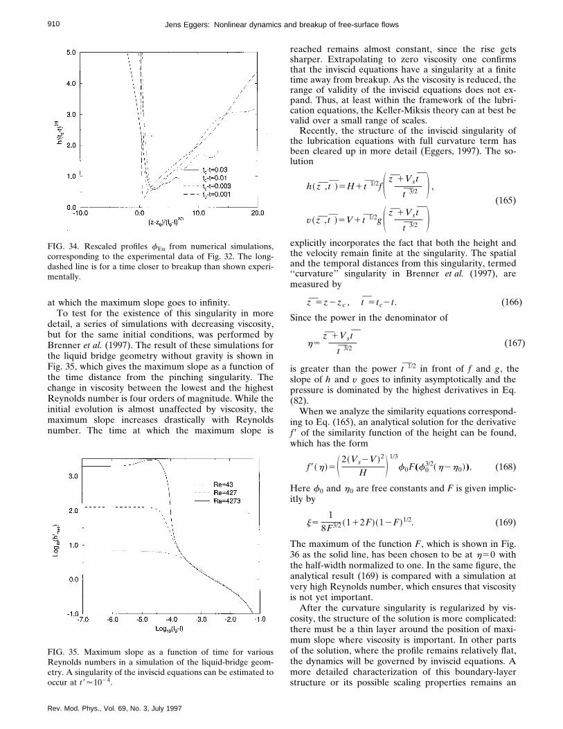
)
910 Jens Eggers: Nonlinear dynamics and breakup of free-surface flows
at which the maximum slope goes to infinity.To test for the existence of this singularity in more
detail, a series of simulations with decreasing viscosity,but for the same initial conditions, was performed byBrenner et al. (1997). The result of these simulations forthe liquid bridge geometry without gravity is shown inFig. 35, which gives the maximum slope as a function ofthe time distance from the pinching singularity. Thechange in viscosity between the lowest and the highestReynolds number is four orders of magnitude. While theinitial evolution is almost unaffected by viscosity, themaximum slope increases drastically with Reynoldsnumber. The time at which the maximum slope is
FIG. 34. Rescaled profiles fEu from numerical simulations,corresponding to the experimental data of Fig. 32. The long-dashed line is for a time closer to breakup than shown experi-mentally.
FIG. 35. Maximum slope as a function of time for variousReynolds numbers in a simulation of the liquid-bridge geom-etry. A singularity of the inviscid equations can be estimated tooccur at t8'1024.
Rev. Mod. Phys., Vol. 69, No. 3, July 1997
reached remains almost constant, since the rise getssharper. Extrapolating to zero viscosity one confirmsthat the inviscid equations have a singularity at a finitetime away from breakup. As the viscosity is reduced, therange of validity of the inviscid equations does not ex-pand. Thus, at least within the framework of the lubri-cation equations, the Keller-Miksis theory can at best bevalid over a small range of scales.
Recently, the structure of the inviscid singularity ofthe lubrication equations with full curvature term hasbeen cleared up in more detail (Eggers, 1997). The so-lution
h~ z , t !5H1 t 1/2fS z 1Vst
t 3/2 D ,
(165)
v~ z , t !5V1 t 1/2gS z 1Vst
t 3/2 Dexplicitly incorporates the fact that both the height andthe velocity remain finite at the singularity. The spatialand the temporal distances from this singularity, termed‘‘curvature’’ singularity in Brenner et al. (1997), aremeasured by
z 5z2zc , t 5tc2t . (166)
Since the power in the denominator of
h5z 1Vst
t 3/2(167
is greater than the power t 1/2 in front of f and g , theslope of h and v goes to infinity asymptotically and thepressure is dominated by the highest derivatives in Eq.(82).
When we analyze the similarity equations correspond-ing to Eq. (165), an analytical solution for the derivativef8 of the similarity function of the height can be found,which has the form
f8~h!5S 2~Vs2V !2
H D 1/3
f0F(f03/2~h2h0!). (168)
Here f0 and h0 are free constants and F is given implic-itly by
j51
8F3/2 ~112F !~12F !1/2. (169)
The maximum of the function F , which is shown in Fig.36 as the solid line, has been chosen to be at h50 withthe half-width normalized to one. In the same figure, theanalytical result (169) is compared with a simulation atvery high Reynolds number, which ensures that viscosityis not yet important.
After the curvature singularity is regularized by vis-cosity, the structure of the solution is more complicated:there must be a thin layer around the position of maxi-mum slope where viscosity is important. In other partsof the solution, where the profile remains relatively flat,the dynamics will be governed by inviscid equations. Amore detailed characterization of this boundary-layerstructure or its possible scaling properties remains an

911Jens Eggers: Nonlinear dynamics and breakup of free-surface flows
open problem. Likewise, the reason for the appearanceof the exponent a52/3, which seems to be selected oversome range of scales, has not been understood on adeeper level.
C. Satellite drops
The understanding of satellite drops and their possiblecontrol has been the driving force behind much of theresearch on drop formation. It seems they were first ob-served by Plateau (1849) in his experiments with an un-stable cylinder of viscous fluid suspended in another (seeFig. 37).
In air, where drops are not held in place by the outerfluid, they are much harder to observe, but still did notescape the attentive eyes of Guthrie (1864). He noticedtiny drops being thrown upward towards the nozzle in adripping-faucet experiment and conjectured that theyresulted from the profile’s not being spherical at thepoint of breakup. Rayleigh (1882), using stroboscopicmethods, saw small drops appearing between maindrops in jet experiments and called them ‘‘spherules.’’For engineering purposes, jets are of particular impor-tance, the ink-jet printer playing the role of a prototypi-cal application (Pimbley and Lee, 1977; Chaudhary andMaxworthy, 1980b). As the drops separate from the inkjet, they are individually charged and deflected ontotheir target by an electric field. The smaller satellites aredeflected differently, producing an undesirable ‘‘halo’’around the intended point. So the goal is to avoid satel-lite formation altogether or to avoid having the satellitescharged.
Under normal circumstances, satellite drops are a uni-versal feature of breakup, quite independent of the ex-
FIG. 36. The similarity function (169) for the inviscid singular-ity of the lubrication equations. Theory is compared with anumerical simulation at Re553109, at a time when the maxi-mum slope has reached 104.
Rev. Mod. Phys., Vol. 69, No. 3, July 1997
perimental configuration. Qualitatively, they comeabout through two properties of the pinching singularity:
(i) The singularity is localized, producing pinchoff at apoint. Since only a small amount of fluid is involved, itacts on time scales much shorter than the growth of dis-turbances on the jet, once it sets in.
(ii) The singularity is asymmetrical, so the only way itcan be matched onto an outer solution is by pinchingnext to a drop, the steep part forming on the side of thedrop, the flat part merging into the flat neck.
Hence the neck is pinched off from either side andeventually contracts into a satellite drop. By lookingback at the sequence of pictures in Fig. 6, one can seethis very clearly. Although the neck is initially thinnestin its middle section, localized pinching sets in only atthe time of the last picture of the first row, after a well-separated drop has begun to form. From this point tobreakup in the next picture the outer part of the solutionhas hardly moved, illustrating the separation of timescales. Before the neck can retract, it pinches on its up-per end, and thus a satellite is formed. The same argu-ments of course apply to jet decay, so within one periodtwo drops are produced, a main drop with volume Vdand a satellite drop with a much smaller volume Vs . Atlong wavelengths the neck becomes very long and is sub-ject to secondary breakings, which we shall disregardhere. We are going to focus on flow at low viscosities,but similar mechanisms are present at higher viscosities,as can be seen in the pictures of ‘‘micro-threading’’ (Fig.30).
The total volume of both main drop and satellite iscontrolled by mass conservation. That is Vd1Vs is equalto the volume of fluid leaving the orifice during one pe-riod, and thus
FIG. 37. The final stages of the breakup of a column of oliveoil in a mixture of alcohol and water, as observed by Plateau(1849).
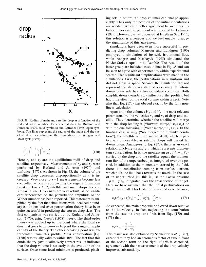
912 Jens Eggers: Nonlinear dynamics and breakup of free-surface flows
S rd
r0D 3
1S rs
r0D 3
53p
2x. (170)
Here rd and rs are the equilibrium radii of drop andsatellite, respectively. Measurements of rd and rs wereperformed by Rutland and Jameson (1970) andLafrance (1975). As shown in Fig. 38, the volume of thesatellite drop decreases disproportionally as x is in-creased. Very close to x51 measurements become lesscontrolled as one is approaching the regime of randombreakup. For x&0.2, satellite and main drops becomesimilar in size. Drop sizes are very robust, as no signifi-cant dependence on the perturbation amplitude or theWeber number has been reported. This statement is am-plified by the fact that simulations with idealized bound-ary conditions and even perturbation theory have beenquite successful in predicting the correct drop sizes. Thefirst comparison was carried out by Rutland and Jame-son (1970), using Yuen’s (1968) theory. The third-ordertheory was applied up to the point where the local ra-dius first goes to zero—way beyond the range of appli-cability of the theory. The other breaking point was ex-trapolated from this profile. Mass conservation [Eq.(170)] was usually valid to within 10%. The fact that thiscrude theory gave qualitatively correct results indicatesthat the drop volume is set early in the evolution of thesurface. Once some local minimum is produced, pinch-
FIG. 38. Radius of main and satellite drop as a function of thereduced wave number. Experimental data by Rutland andJameson (1970, solid symbols) and Lafrance (1975, open sym-bols). The lines represent the radius of the main and the sat-ellite drop according to the simulations by Ashgriz andMashayek (1995).
Rev. Mod. Phys., Vol. 69, No. 3, July 1997
ing sets in before the drop volumes can change appre-ciably. Thus only the position of the initial indentationsare needed. An even better agreement between pertur-bation theory and experiment was reported by Lafrance(1975). However, as we discussed at length in Sec. IV.C,this solution is erroneous and we feel unable to judgethe significance of this agreement.
Simulations have been even more successful in pre-dicting drop volumes. Mansour and Lundgren (1990)employed a simulation of inviscid, irrotational flow,while Ashgriz and Mashayek (1995) simulated theNavier-Stokes equation at Re=200. The results of thelatter group are included as solid lines in Fig. 38 and canbe seen to agree with experiment to within experimentalscatter. Two significant simplifications were made in thesimulations: First, the perturbations were uniform anddid not grow in space. Second, the simulation did notrepresent the stationary state of a decaying jet, whosedownstream side has a free-boundary condition. Bothsimplifications considerably influenced the profiles, buthad little effect on the total volume within a neck. Notealso that Eq. (170) was obeyed exactly by the fully non-linear calculation.
Apart from the volumes Vd and Vs , the most relevantparameters are the velocities vd and vs of drop and sat-ellite. They determine whether the satellite will mergewith the drop leading it (‘‘forward merge,’’ vs.vd) orwith the one following it (‘‘rear merge,’’ vs,vd). In thelimiting case vs5vd (‘‘no merge’’ or ‘‘infinity condi-tion’’), the satellite will not merge at all, which is par-ticularly undesirable, as satellite drops will persist fardownstream. Analogous to Eq. (170), there is an exactrelation involving vd and vs , which represents momen-tum conservation. In it, the momentum r(vdVd1vsVs)carried by the drop and the satellite equals the momen-tum flux of the unperturbed jet, integrated over one pe-riod. In addition to the momentum carried by the fluid,there is a contribution coming from surface tension,which pulls the fluid back towards the nozzle. In the caseof an unperturbed jet, this is just the excess pressure2p52g/r0, integrated over the cross section of the jet.Here we have assumed that the initial perturbations onthe jet are small. This leads to the second exact balance,
v j~rd3vd1rs
3vs!53p
2x S v j2r0
32g
rr0
2D . (171)
As expected, the main drop will be slowed down relativeto the jet velocity. In fact, neglecting the contributionfrom the satellite drop, one finds from Eqs. (170) and(171) that
vd'v j2g
r
1r0v j
.
This result was also obtained by Schneider et al. (1967),except that they had an erroneous factor of two in frontof the second term on the right. If this is corrected,agreement with their measurements of the drop velocityimproves substantially.
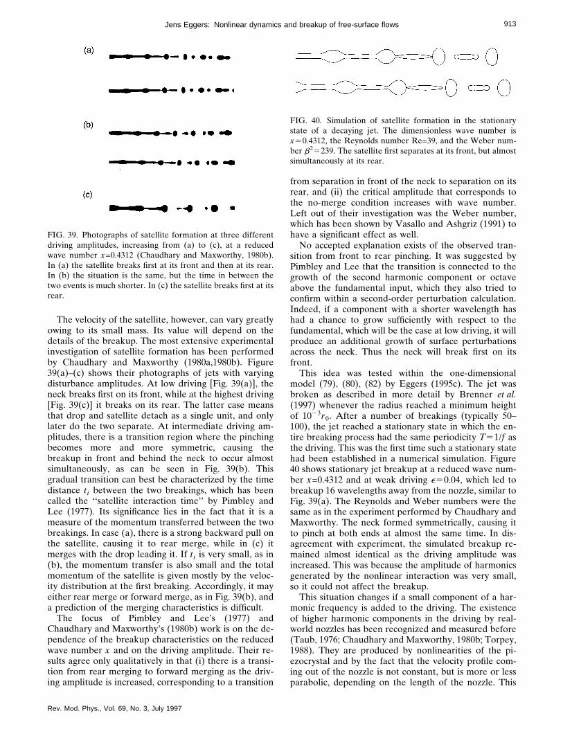
913Jens Eggers: Nonlinear dynamics and breakup of free-surface flows
The velocity of the satellite, however, can vary greatlyowing to its small mass. Its value will depend on thedetails of the breakup. The most extensive experimentalinvestigation of satellite formation has been performedby Chaudhary and Maxworthy (1980a,1980b). Figure39(a)–(c) shows their photographs of jets with varyingdisturbance amplitudes. At low driving [Fig. 39(a)], theneck breaks first on its front, while at the highest driving[Fig. 39(c)] it breaks on its rear. The latter case meansthat drop and satellite detach as a single unit, and onlylater do the two separate. At intermediate driving am-plitudes, there is a transition region where the pinchingbecomes more and more symmetric, causing thebreakup in front and behind the neck to occur almostsimultaneously, as can be seen in Fig. 39(b). Thisgradual transition can best be characterized by the timedistance t i between the two breakings, which has beencalled the ‘‘satellite interaction time’’ by Pimbley andLee (1977). Its significance lies in the fact that it is ameasure of the momentum transferred between the twobreakings. In case (a), there is a strong backward pull onthe satellite, causing it to rear merge, while in (c) itmerges with the drop leading it. If t i is very small, as in(b), the momentum transfer is also small and the totalmomentum of the satellite is given mostly by the veloc-ity distribution at the first breaking. Accordingly, it mayeither rear merge or forward merge, as in Fig. 39(b), anda prediction of the merging characteristics is difficult.
The focus of Pimbley and Lee’s (1977) andChaudhary and Maxworthy’s (1980b) work is on the de-pendence of the breakup characteristics on the reducedwave number x and on the driving amplitude. Their re-sults agree only qualitatively in that (i) there is a transi-tion from rear merging to forward merging as the driv-ing amplitude is increased, corresponding to a transition
FIG. 39. Photographs of satellite formation at three differentdriving amplitudes, increasing from (a) to (c), at a reducedwave number x=0.4312 (Chaudhary and Maxworthy, 1980b).In (a) the satellite breaks first at its front and then at its rear.In (b) the situation is the same, but the time in between thetwo events is much shorter. In (c) the satellite breaks first at itsrear.
Rev. Mod. Phys., Vol. 69, No. 3, July 1997
from separation in front of the neck to separation on itsrear, and (ii) the critical amplitude that corresponds tothe no-merge condition increases with wave number.Left out of their investigation was the Weber number,which has been shown by Vasallo and Ashgriz (1991) tohave a significant effect as well.
No accepted explanation exists of the observed tran-sition from front to rear pinching. It was suggested byPimbley and Lee that the transition is connected to thegrowth of the second harmonic component or octaveabove the fundamental input, which they also tried toconfirm within a second-order perturbation calculation.Indeed, if a component with a shorter wavelength hashad a chance to grow sufficiently with respect to thefundamental, which will be the case at low driving, it willproduce an additional growth of surface perturbationsacross the neck. Thus the neck will break first on itsfront.
This idea was tested within the one-dimensionalmodel (79), (80), (82) by Eggers (1995c). The jet wasbroken as described in more detail by Brenner et al.(1997) whenever the radius reached a minimum heightof 1023r0. After a number of breakings (typically 50–100), the jet reached a stationary state in which the en-tire breaking process had the same periodicity T51/f asthe driving. This was the first time such a stationary statehad been established in a numerical simulation. Figure40 shows stationary jet breakup at a reduced wave num-ber x=0.4312 and at weak driving e50.04, which led tobreakup 16 wavelengths away from the nozzle, similar toFig. 39(a). The Reynolds and Weber numbers were thesame as in the experiment performed by Chaudhary andMaxworthy. The neck formed symmetrically, causing itto pinch at both ends at almost the same time. In dis-agreement with experiment, the simulated breakup re-mained almost identical as the driving amplitude wasincreased. This was because the amplitude of harmonicsgenerated by the nonlinear interaction was very small,so it could not affect the breakup.
This situation changes if a small component of a har-monic frequency is added to the driving. The existenceof higher harmonic components in the driving by real-world nozzles has been recognized and measured before(Taub, 1976; Chaudhary and Maxworthy, 1980b; Torpey,1988). They are produced by nonlinearities of the pi-ezocrystal and by the fact that the velocity profile com-ing out of the nozzle is not constant, but is more or lessparabolic, depending on the length of the nozzle. This
FIG. 40. Simulation of satellite formation in the stationarystate of a decaying jet. The dimensionless wave number isx50.4312, the Reynolds number Re=39, and the Weber num-ber b25239. The satellite first separates at its front, but almostsimultaneously at its rear.

914 Jens Eggers: Nonlinear dynamics and breakup of free-surface flows
inevitably translates into nonsinusoidal modulations ofthe jet. The effect of a nontrivial velocity profile on thejet evolution has been studied directly in an interestingpaper by Razumovski� (1993).
The effect of the second harmonic with 1/10 of theamplitude of the fundamental is shown in Fig. 41(a). Ata reduced wave number of 0.4312 the growth of the sec-ond harmonic is faster than that of the fundamental ac-cording to linear theory. Thus at low driving, when thereis sufficient time for the harmonic to grow, it may havean appreciable effect. Indeed, the profiles look remark-ably similar to the experimental ones of Fig. 39(a),which are also at low driving. There is considerablegrowth of surface perturbations across the neck, causingit to separate at its front, while there is not much inden-tation yet on its rear. Note that according to lineartheory the amplitude of the second harmonic should stillbe 1/6 of the fundamental at breakup, so nonlinear ef-fects must also play an important role. If the input isstronger, but the amplitude ratio of the second harmonicto the fundamental is kept constant [see Fig. 41(b)], theharmonic has much less time to grow. Thus the breakupresembles the one without higher harmonic driving (Fig.40), being much more symmetric [see Fig. 41(b)]. Thistransition to symmetric pinching with increased drivingamplitude is similar to experimental observation [seeFig. 39(a),(b)]. Increasing the driving amplitude still fur-ther does not produce any change in the simulations, asthe second harmonic has already become irrelevant. Ac-cordingly, no breakup was found corresponding to Fig.39(c), which represents the highest experimental drivingamplitude. It seems as if the jet profile is severely dis-torted even two wavelengths before breakup, indicatinga strong increase in nonharmonic input, which was notaccounted for in the simulations.
Thus we have seen that even small changes in the
FIG. 41. Same as in Fig. 40, but with the second harmoniccomponent with 1/10 of the amplitude of the fundamentaladded. Part (a) shows the case of low driving, (b) the case ofhigher driving. A transition to almost symmetrical pinching isobserved.
Rev. Mod. Phys., Vol. 69, No. 3, July 1997
driving have a significant effect on breakup. Increasingthe driving amplitude leads to a transition to symmetricpinching in both simulation and experiment. However,too little is known about the actual experimental drivingto draw more definite conclusions.
VIII. RELATED PROBLEMS
For the last section we have selected three more gen-eral problems, which stand out not only for their fasci-nating physics, but also for their technological impor-tance. The dynamics of two-fluid systems governs mixingprocesses. Here the assumption of a free boundary isabandoned. Shearing forces act on the piece of fluidabout to break up, and the dynamics of the outer fluidhave to be considered as well. Electrically driven jets arebeing used for the production of sprays of very smalldrops of uniform size, and of charged macromolecules inthe gas phase. These jets generically appear when a po-larizable fluid is placed in a strong electric field. Finally,liquids containing macromolecules are ubiquitous in in-dustrial processing such as fiber spinning. Macromol-ecules have long time scales associated with their distor-tion and relaxation, which interfere with the time scalesrelevant for breakup. This and their highly anisotropicviscosity fundamentally alters the behavior nearbreakup.
A. Two-fluid systems
Here we consider the dynamics and breakup of a dropof fluid in another fluid, which is considered to be un-bounded. In the case of breakup in air, both the viscosityand the density of the gas are usually negligible, but forfluids the dynamics change. First, the outer fluid has tomove with the inner fluid, and second it exerts a forcethrough its shear stresses. This is true even if the outerfluid is at rest, but if in addition there is a nontrivialouter flow, it acts as an external forcing that deforms thedrop.
The main interest in the subject comes from the prob-lem of mixing. Figure 42 shows how a single drop isquickly dispersed into a large number of small droplets,which are distributed almost evenly throughout the con-tainer. First the drop is stretched into a long filament.Even though it becomes very thin, it remains remark-ably stable against capillary instability. Owing to thecomplicated structure of Lagrangian trajectories even insimple flows, the filament is folded into an intricatestructure. In certain parts of the flow the filament finallybreaks up into drops under the action of surface tension,and the container is soon filled with tiny drops.
It was G. I. Taylor’s idea to break up this extremelycomplicated phenomenon into a number of simplerones, two of which he hoped would depend only on thelocal properties of the flow field, namely, the deforma-tion and stretching of drops and the breakup of longfilaments. Only the folding depends on the global struc-ture of the flow, and indeed the chaotic motion of La-grangian paths is a research subject in its own right, not

915Jens Eggers: Nonlinear dynamics and breakup of free-surface flows
FIG. 42. Dynamics of elongation, folding, andbreakup of a drop placed in the globally cha-otic flow produced in a time-periodicallymodulated eccentric journal bearing. Thedrop is less viscous than the surrounding fluidby a factor of l50.067 (Tjahjadi and Ottino,1991). Reprinted with permission of Cam-bridge University Press.
to be considered here. The fundamental approach in allof the following is to look at a single drop or filamentand to assume its dimensions to be small compared withthe typical scale of the outer flow. Thus the outer flowcan be treated in a linear approximation
v5G•x512
v3x1D•x, (172)
where v is the vorticity, D the deformation tensor, andGT the velocity gradient tensor. Moreover, in almost allof the work on the problem to date the drop is assumedto be small enough for the Reynolds number to be smallin both fluids, so that the Stokes approximation is appli-cable.
In his first two papers Taylor (1932, 1934) looked atthe stationary shape and the stability of drops in twoprototypical flows. One is a purely extensional flow withzero vorticity, the other a simple shear flow. At a criticalflow rate, which depends on the viscosity ratio betweenthe two fluids, the stationary drop becomes unstable andstarts to stretch. This situation was investigated by To-motika (1936), who explained the surprising stability of
Rev. Mod. Phys., Vol. 69, No. 3, July 1997
cylindrical filaments in the process of stretching. Whenthe flow is turned off, or in the context of mixing, if thefilament is convected into a region of low strain rate, it isprone to capillary instability, which was investigated inan earlier paper (Tomotika, 1935). The capillary insta-bility and the subsequent nonlinear evolution were in-vestigated both experimentally and numerically by Lealand co-workers, and are summarized in the review paperby Stone (1994).
1. Stationary shapes
As suggested by Taylor, we are looking at the case ofa linear flow field, either two-dimensional extensionalflow
G5GF 1 0 0
0 21 0
0 0 0G , (173)
or simple shear flow

916 Jens Eggers: Nonlinear dynamics and breakup of free-surface flows
G5G
2 F 0 1 0
0 0 0
0 0 0G . (174)
If the undisturbed drop radius is a , then the static prob-lem is governed by the viscosity contrast
l5h8
h, (175)
which measures the viscosity of the drop h8 relative tothat of the outer fluid h , and the capillary number
Ca5Gha
g, (176)
which measures the strength of the external shearingforces relative to the surface tension forces. The Rey-nolds number is assumed to be small and the drop fluidis chosen to be neutrally buoyant, r85r .
For increasingly large capillary numbers, the drop de-forms more and more, as measured by the ratio of thehalf-widths, L/B . The outer flow stretches small distur-bances on the surface, so the drop is stable against cap-illary instability even if it is long and thin. The strain rateat which drops can exist in equilibrium is limited ratherby the pressure, which builds up at the end of the drop.Here, fluid is being pushed toward the tip, and a pres-sure gradient maintains the necessary backflow. At somecritical capillary number the pressure at the end of thedrop overcomes capillary pressure, the drop becomesunstable, and it starts to stretch with the flow. Thesmaller the viscosity of the drop, the smaller the pres-sure needed to maintain the backflow, and the more ex-tended the drops become before they start to extend. Inextensional flow, for any viscosity ratio there is a criticalcapillary number that breaks the drop. If vorticity ispresent, as in the flow (174), drops of high viscosity be-have in radically different ways, as discovered by Taylor(1934). For l*4 the drop performs a solid-body rota-tion, thus evading the shearing forces, and no longerbreaks up even at the highest capillary numbers. Thus adrop of a high viscosity fluid must be mixed by entirelydifferent means from those of Fig. 42.
Figure 43 shows drops at the critical capillary numberfor two different viscosity ratios in an extensional flow.At the higher viscosity the drop is still close to sphericalat the point of instability, so it can be described in anexpansion around this shape. On the other hand, forvery long drops of low viscosity ratio, Taylor (1966) pro-posed an expansion for small B/L , very similar to thelubrication expansions of Sec. V. Taylor’s ideas weresubsequently developed into a fairly complete theory ofequilibrium shapes by A. Acrivos and his associates(Barthes-Biesel and Acrivos, 1973; Acrivos and Lo,1978; Rallison and Acrivos, 1978; Hinch and Acrivos,1979, 1980).
Barthes-Biesel and Acrivos (1973) carried the expan-sion for small deformation to second order and used itto predict both drop shapes and critical capillary numberat large l . Buckmaster (1972) investigated the opposite
Rev. Mod. Phys., Vol. 69, No. 3, July 1997
limit of an inviscid bubble and found a family of elon-gated shapes with pointed ends by using slender-bodytheory. Later, Acrivos and Lo (1978) singled out oneshape,
h~z !5a
4CaF12S z
20aCa2D 2G , (177)
as the only stable solution. They also generalized theprevious results to viscous drops, which allowed them tofind the critical capillary number as a function of l!1:
Cacrl1/650.148. (178)
In particular, this means that an inviscid drop never be-comes unstable and can be stretched to arbitrarylengths. Hinch and Acrivos (1979, 1980) removed thesimplifying assumption of axisymmetry in these calcula-tions, but found the results to be fundamentally thesame. The theoretical results were checked against nu-merical calculations by Rallison and Acrivos (1978) andagainst experiments by Bentley and Leal (1986a, 1986b).Good agreement was found both in the shapes and inthe critical capillary number, as long as the deformationwas either small or very large.
The major unsolved problem connected with thetheory of stationary shapes concerns the solution (177),valid for very elongated and almost inviscid bubbles.Equation (177) predicts a pointed conical tip at the endof the bubble, in agreement with experiment (see Fig.43). Thus one would have a singularity of the curvatureat the end. However, Buckmaster (1972) used a localanalysis to show that conical tips are in fact not a solu-tion of the equations, so the expansion leading to Eq.(177) has to break down near the tip. In light of ouranalysis of a receding tip in Sec. VI.D this may not besurprising, as lubrication equations should be expectedto break down near a tip. Buckmaster (1972) estimatedthe size of the region where lubrication theory breaksdown to be of the order of exp@2Ca6#. In this break-down lies a tantalizing analogy to two-dimensionalStokes flow, which produces an apparent cusp of a freesurface (Joseph et al., 1991). Here the shear needed toform the cusp is produced by two rollers submerged un-der the surface of a tank of viscous fluid. An exact solu-
FIG. 43. Two examples of drops in an extensional flow at thecritical capillary number. The top picture shows a highly vis-cous drop (l524.5), which is still ellipsoidal at the criticalcapillary number of Cacr50.106. The bottom picture shows ahighly deformed drop with l51.0531023 at Cacr50.457. Notethe pointed ends. From Bentley and Leal, 1986b. Reprintedwith permission of Cambridge University Press.

917Jens Eggers: Nonlinear dynamics and breakup of free-surface flows
tion of a slightly idealized problem was found (Jeongand Moffatt, 1992), which shows that the cusp singular-ity is actually regularized by surface tension close to thetip, forming a rounded end with a radius of curvatureexponentially small in the capillary number. The samehas been suspected by Sherwood (1981) to happen in thepresent problem, but no solution has been found yet.
But the analogy does not stop here. As the capillarynumber is increased in the two-roller apparatus, a thinsheet of air emanates from the cusp (Moffatt, 1995), thusentraining air into the fluid. A very similar phenomenonhad already been observed by Taylor (1934) in the axi-symmetric case and goes by the name of ‘‘tip stream-ing.’’ A thin jet of fluid is ejected from the tip, whichsoon breaks up into droplets due to the Rayleigh insta-bility, as can be seen in Fig. 44. A theoretical explana-tion of this phenomenon does not exist. Sherwood(1984) suggests that the tip is unstable owing to nonlin-earities in the outer flow, and gives some very clear ex-perimental pictures. de Bruijn (1993) experimentally in-vestigates the influence of surfactants and finds that theappearance of tip streaming crucially depends on thetype of fluid used. Most importantly, he finds that tipstreaming ceases after a certain period of time, possibly
FIG. 44. Tip streaming in a Couette device at a shear rate of19.5 s21. Shown is a drop of water in silicone oil which is 1000times as viscous. To initiate tip streaming, 200 ppm of surfac-tant has been added. The image width is 0.5 mm (Leonhard,1996).
Rev. Mod. Phys., Vol. 69, No. 3, July 1997
after a surfactant is depleted from the tip. If the drop isleft at rest for a while, tip streaming commences. Addinga surfactant provokes tip streaming in fluids that ordi-narily show no tip streaming. de Bruijn also observes avariety of hysteresis effects as the shear rate is varied.From this it is clear that surfactants have an important ifnot essential effect on tip streaming. However, it is notobvious that they are really needed to explain the phe-nomenon, or whether they just enhance the effect. Forexample, without surfactant the jet might be too thin tobe observed or it only appears at much higher shearrates. In any case, a more complete analysis of the tipregion even before the onset of tip streaming seems likean obvious first step towards an understanding.
2. Breakup
As mentioned before, the growth of perturbations ona fluid filament that stretches at a uniform rate was in-vestigated by Tomotika (1936). As the filament isstretched, the wavelength of the perturbation increases.Its amplitude relative to the radius of the filament in-creases by only a finite factor, even as the radius goes tozero. However, this factor may be large if the perturba-tion is introduced at a later stage of the stretching,where the filament is already thinner. Thus, although therelative growth remains finite in the linear approxima-tion, this may be enough to break the filament. But onlywhen the flow is turned off or the flow rate is substan-tially reduced does exponential growth set in (Tomotika,1935; Mikami, Cox, and Mason, 1975). Growth rates andmaximum unstable wavelength depend on the viscosityratio l .
As the amplitude of perturbations increases, nonlin-ear effects become important. They have been studied ina series of papers (Stone, Bentley, and Leal, 1986; Stoneand Leal, 1989a, 1989b; Tjahjadi, Stone, and Ottino,1992) experimentally and in parallel simulations. In ad-dition to breakup driven by the Rayleigh instability, anew type of breakup was observed, called ‘‘end pinch-ing.’’ As depicted in Fig. 45, as the filament contracts,two bulbous heads form at the end of the filament; theythen separate while the rest of the filament remains in-tact. Only later does the filament break into many smalldrops under the action of the Rayleigh instability. Formoderately extended filaments, L/a,20, end pinching isin fact the dominant effect and the filament contracts toa drop before capillary breakup sets in.
Therefore, to observe capillary breakup without inter-ference from finite size effects, filaments have to bestretched considerably. This was done by Tjahjadi,Stone, and Ottino (1992) using a flow between two con-centric cylinders. If the viscosity ratio l is high, then theouter fluid can be neglected and one is back at the physi-cal situation of the previous sections. The final state af-ter the breakup of such a filament is shown in the bot-tom picture of Fig. 46, with matching simulations ofStokes flow. Note the agreement with Fig. 37, published140 years earlier. Apart from the main satellite formedby the bulbous neck, another much smaller satellite is

918 Jens Eggers: Nonlinear dynamics and breakup of free-surface flows
found on either side of it. The reason is that as the fluidpinches at the main drop, a conical neck is left behind.As this neck retracts, it tends to form a bulbous part,which again is prone to pinching.
FIG. 45. Extension and subsequent relaxation of a drop atl50.046. After the flow is stopped, the filament first under-goes end pinching and then decays into equally spaced dropscorresponding to the most unstable wavelength (Stone, Bent-ley, and Leal, 1986). Reprinted with permission of CambridgeUniversity Press.
Rev. Mod. Phys., Vol. 69, No. 3, July 1997
As the viscosity ratio is decreased, the final structurebecomes ever more intricate, as can be seen by goingtowards the top of Fig. 46. Even on very small scales, areceding neck has a chance to form a bulbous sectionbefore it can completely retract, and the process ofpinching becomes self-repeating. For the smallest l , sat-ellite drops lie on an intricate fractal structure, thesmallest drops observed experimentally having a size of10 mm. It seems likely that for finite l there is a cutoffbelow which no further pinching takes place, but an es-timate is not known.
Up to now we have considered only the nonlinear be-havior away from the pinch point. As the neck becomesthinner, one expects scale-invariant solutions to appear.However, the force balance cannot be the same as in thefree boundary case, and new power laws appear. Thereason is that, in the case of a free boundary, viscousstresses are given by hDv/l z
2 , where Dv is a typical ve-locity scale and l z an axial scale. If an outer fluid ispresent, there must be a boundary layer of the outerfluid over which the velocity at the interface falls off tozero. This is essentially a radial scale, so viscous stressesare now h8Dv/l r
2 . Since in the asymptotic solutionswith free boundary l r goes to zero faster than l z , vis-cous stresses due to the outer fluid will eventually domi-nate, thus changing the force balance. Inevitably, the ex-ponents describing this new solution will also bedifferent. Thus, strictly speaking, even for an outer fluidwith very small viscosity h8, the scaling laws will even-tually cross over to this new type of scaling.
FIG. 46. Breakup of a filament into satellite and subsatellite drops. As the viscosity ratio l is decreased, the final state of thesystem has an increasingly complicated fractal structure (Tjahjadi, Stone, and Ottino, 1992). The pictures are, from top to bottom,for l = 0.01, 0.067, 0.4, 1, and 2.8. Reprinted with permission of Cambridge University Press.

919Jens Eggers: Nonlinear dynamics and breakup of free-surface flows
FIG. 47. A drop of water, 1.5 cm in diameter, subject to a strong electric field of 6 kvolts/cm in a zero-gravity environment. In (a)the free-floating drop is shown, while the other frames show the drop 3, 6, and 9 ms after the electric field has been turned on(Inculet and Floryan, 1990).
The difficulty in setting up asymptotic equations ofmotion for this problem lies in the fact that the flow isunbounded. Therefore there is no obvious expansion ina small parameter like the slenderness ratio of thethread. Rather, further knowledge of the boundary layeraround the filament is required. One can expect, how-ever, that close to the singularity the contribution fromthe outer fluid is local as well, in that only flow fromclose to the point of breaking has to be taken into ac-count. In the case of Stokes flow, some steps have beentaken in the direction of ‘‘localizing’’ the contributionfrom the outer flow (Lister and Stone, 1996; Lister,Stone, and Brenner, 1997), but a self-similar descriptionof the singularity remains a challenging problem.
B. Electrically driven jets
When a dielectric drop is placed in an electric field, itbecomes polarized and the induced surface charges arepulled apart. Thus a more elongated equilibrium shapeis reached, which depends on the field strength. Zeleny(1914, 1915, 1917) discovered that when the electric fieldstrength is raised above a critical value, these shapesbecome unstable and a conical tip appears at the end ofthe drop, from which a tiny jet is ejected. Taylor (1964)showed that a cone is a local equilibrium solution inwhich surface tension and electric forces are balanced.These cones, which have a definite opening angle of98.6°, are known as Taylor cones. Thus, once more wefind a phenomenon in which a surface singularity is
Rev. Mod. Phys., Vol. 69, No. 3, July 1997
formed under the influence of external forces and whichthen gives birth to a jet or a channel. Similar stretchingof a drop and the formation of pointed spikes is ob-served with ferrofluids in a magnetic field (Cowley andRosensweig, 1967; Bacri and Salin, 1982).
Two different experimental setups are commonlyused. In one, the dielectric fluid is released from a metalcapillary tube, which is placed opposite an electrode ona fixed potential relative to the tube. This configurationis used in engineering applications. Gravity can be com-pensated by the pressure in the tube, and new fluid canbe introduced at will. This setup, which readily allowsfor the formation of electrically driven jets, has gainedvast importance in the production of sprays (Bailey,1988). Recently, the same technique has been used toproduce ions of macromolecules in the gas phase andhas revolutionized mass spectrometry of such molecules(Fenn et al., 1989).
Despite its great importance, little is known theoreti-cally about the formation of such electrically driven jetsor the parameters controlling its properties or stability.For this reason, it is preferable to look at a simplersetup, in which parameters like the geometry of themetal tube, flow rates, or contact angles do not appear.This second common experimental setup consists of anisolated drop placed between two capacitor plates,which produce a uniform electric field. Gravity is elimi-nated either by using a neutrally buoyant drop (Taylor,1964) or by placing the drop in a zero-gravity environ-ment (Inculet and Floryan, 1990). Figure 47 shows a se-
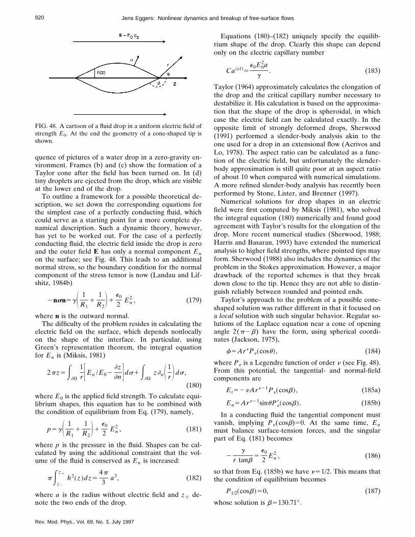
920 Jens Eggers: Nonlinear dynamics and breakup of free-surface flows
quence of pictures of a water drop in a zero-gravity en-vironment. Frames (b) and (c) show the formation of aTaylor cone after the field has been turned on. In (d)tiny droplets are ejected from the drop, which are visibleat the lower end of the drop.
To outline a framework for a possible theoretical de-scription, we set down the corresponding equations forthe simplest case of a perfectly conducting fluid, whichcould serve as a starting point for a more complete dy-namical description. Such a dynamic theory, however,has yet to be worked out. For the case of a perfectlyconducting fluid, the electric field inside the drop is zeroand the outer field E has only a normal component Enon the surface; see Fig. 48. This leads to an additionalnormal stress, so the boundary condition for the normalcomponent of the stress tensor is now (Landau and Lif-shitz, 1984b)
2nsn5gS 1R1
11
R2D1
e0
2En
2 , (179)
where n is the outward normal.The difficulty of the problem resides in calculating the
electric field on the surface, which depends nonlocallyon the shape of the interface. In particular, usingGreen’s representation theorem, the integral equationfor En is (Miksis, 1981)
2pz5E]V
1r FEn /E02
]z
]nGds1E]V
z]nS 1r Dds ,
(180)
where E0 is the applied field strength. To calculate equi-librium shapes, this equation has to be combined withthe condition of equilibrium from Eq. (179), namely,
p5gS 1R1
11
R2D1
e0
2En
2 , (181)
where p is the pressure in the fluid. Shapes can be cal-culated by using the additional constraint that the vol-ume of the fluid is conserved as En is increased:
pEz2
z1
h2~z !dz54p
3a3, (182)
where a is the radius without electric field and z6 de-note the two ends of the drop.
FIG. 48. A cartoon of a fluid drop in a uniform electric field ofstrength E0. At the end the geometry of a cone-shaped tip isshown.
Rev. Mod. Phys., Vol. 69, No. 3, July 1997
Equations (180)–(182) uniquely specify the equilib-rium shape of the drop. Clearly this shape can dependonly on the electric capillary number
Ca ~el !5e0E0
2a
g. (183)
Taylor (1964) approximately calculates the elongation ofthe drop and the critical capillary number necessary todestabilize it. His calculation is based on the approxima-tion that the shape of the drop is spheroidal, in whichcase the electric field can be calculated exactly. In theopposite limit of strongly deformed drops, Sherwood(1991) performed a slender-body analysis akin to theone used for a drop in an extensional flow (Acrivos andLo, 1978). The aspect ratio can be calculated as a func-tion of the electric field, but unfortunately the slender-body approximation is still quite poor at an aspect ratioof about 10 when compared with numerical simulations.A more refined slender-body analysis has recently beenperformed by Stone, Lister, and Brenner (1997).
Numerical solutions for drop shapes in an electricfield were first computed by Miksis (1981), who solvedthe integral equation (180) numerically and found goodagreement with Taylor’s results for the elongation of thedrop. More recent numerical studies (Sherwood, 1988;Harris and Basaran, 1993) have extended the numericalanalysis to higher field strengths, where pointed tips mayform. Sherwood (1988) also includes the dynamics of theproblem in the Stokes approximation. However, a majordrawback of the reported schemes is that they breakdown close to the tip. Hence they are not able to distin-guish reliably between rounded and pointed ends.
Taylor’s approach to the problem of a possible cone-shaped solution was rather different in that it focused ona local solution with such singular behavior. Regular so-lutions of the Laplace equation near a cone of openingangle 2(p2b) have the form, using spherical coordi-nates (Jackson, 1975),
f5ArnPn~cosu!, (184)
where Pn is a Legendre function of order n (see Fig. 48).From this potential, the tangential- and normal-fieldcomponents are
Et52nArn21Pn~cosb!, (185a)
En5Arn21sinuPn8~cosb!. (185b)
In a conducting fluid the tangential component mustvanish, implying Pn(cosb)50. At the same time, Enmust balance surface-tension forces, and the singularpart of Eq. (181) becomes
2g
r tanb5
e0
2En
2 , (186)
so that from Eq. (185b) we have n51/2. This means thatthe condition of equilibrium becomes
P1/2~cosb!50, (187)
whose solution is b5130.71°.

921Jens Eggers: Nonlinear dynamics and breakup of free-surface flows
Thus one ends up with a very definite answer, whichwas confirmed by Taylor in his experiments with a con-ducting fluid [see Fig. 49(a)], but using electrodes with ashape adjusted to the form of the local solution. Indeed,Eq. (186) requires a definite value of the electric fieldstrength at a given distance from the vertex, and it is notclear under what conditions this local field is consistentwith the applied field E0 and the shape of the drop. Afirst step to investigate this problem was taken by Li,Halsey, and Lobkovsky (1994), who computed the en-ergy of a drop with a trial shape, having two pointedends, in a homogeneous electric field and found it to belower than that of the corresponding ellipsoidal shape.However, there is no reason to believe that their trialshapes are actually solutions of the equations. The localcone-shaped solutions were incorporated in a numericalscheme for solving Eqs. (180)–(182) by Pantano, Gan an-Calvo, and Barrero (1994). Using the geometry of a cap-illary tube facing a capacitor plate, they found stationarysolutions with pointed tips for a range of values ofCa(el) and a .
Li, Halsey, and Lobkovsky (1994) also advance asimple argument that a drop with pointed ends could notcorrespond to a stable equilibrium. That is, a reductionof the cone angle would increase the field strength, elon-gating the end even more. Conversely, an increase of theangle would reduce the field strength, so perturbations
FIG. 49. Three successive frames (in intervals of 1/64 s) show-ing a drop of water (which appears bright) forming a Taylorcone surrounded by oil. The first frame shows a comparisonwith the theoretical prediction of the cone angle; the otherframes show the drop in two phases of its oscillation aroundthis cone (Taylor, 1964). Reprinted with permission of theRoyal Society.
Rev. Mod. Phys., Vol. 69, No. 3, July 1997
of that sort would grow as well. This instability is con-sistent with experimental observations, in which periodicoscillations of the cone angle are observed, the tip beingmore pointed than the static solution in one phase, andmore rounded in the other, see Fig. 49(b),(c). In thepointed phase a jet is ejected from the tip, which is toothin to be resolved in the photograph of Fig. 49.
For other fluids or field strengths, the combined sys-tem of a cone and the jet issuing from its tip is stable.Yet it is not known which parameters are controllingthis behavior and what dynamical mechanism is respon-sible for the stability. It has been suggested that a finiteconductivity of the fluid is essential for stability (Hayati,Bailey, and Tadros, 1986, 1987). A finite tangential elec-tric field produces shear stresses on the surface thatdrive a circulatory motion in the fluid, which might beimportant for stability. Shear stresses on the surfacehave also been discussed in connection with the stabilityof the jet away from the apex of the cone (Mestel, 1994).In fact it is another open question originally addressedby Taylor (1969) why an electrically driven jet is farmore stable than estimates based on the Rayleigh insta-bility would suggest. Taylor investigated the influence ofsurface charges and found them to have stabilizing aswell as destabilizing effects, depending on wave number.Thus the presence of surface charges alone cannot ac-count for the observed stability.
So far it is not even known what sets the scale of thejet radius. As conductivity increases, meaning thatcharge relaxation becomes faster relative to the timescale of the fluid motion, the radius of the jet decreases.In the extreme case of liquid metals, the size of the jetdecreases to the point where single ions are emitted(Gabovich, 1983). Some phenomenological theories, re-lating, for example, the mass flux and the currentthrough an electrical jet, have been proposed by Fernan-dez de la Mora and Loscertales (1994). The gas sur-rounding the Taylor cone is also known to have an im-portant effect (Aguirre-de-Carcer and Fernandez de laMora, 1995).
Nevertheless, despite some advances, the understand-ing of electrically driven jets remains quite rudimentary.Given the success of one-dimensional models in the de-scription of free jets, it seems promising to include anouter electric field to formulate a minimal dynamicmodel. Interesting questions are both the approach tothe Taylor cone in a strong electric field and the dynam-ics of the cone-jet system. Again we restrict ourselves tothe case of a perfectly conducting fluid, where no modelfor charge transport has to be considered. The electricfield is given solely by electrostatics. A comparison be-tween Eqs. (179) and (19) shows that in that case thepressure as given by Eq. (82) has to be replaced by
p5gS 1h~11h82!1/2 2
h9
~11h82!3/2D1e0
2En
2 . (188)
The normal-field component has to be calculated fromEq. (180). Thus in the resulting system (79), (80) allpoints are nonlocally coupled. Even if this model provestoo simple to describe all the experimental effects, and

922 Jens Eggers: Nonlinear dynamics and breakup of free-surface flows
we have mentioned plenty of evidence for this, it willprovide a simple starting point for the exploration of thedynamics. Numerical investigations of Eqs. (79), (80),(180), and (188) are under way (Brenner, 1997).
C. Polymeric liquids
In this final subsection we turn to liquids that haverheological properties different from the Newtonian flu-ids described by the Navier-Stokes equation. This hap-pens whenever the fluid contains macromolecules, evenif they are present in only minute concentrations. It goeswithout saying that such fluids are ubiquitous in chemi-cal processing, so it is essential to understand their non-linear dynamics, which are fundamentally different fromthose of the Newtonian fluids discussed before. Twoproperties are responsible for this: First, polymerschange the viscosity of the suspension by changing theirshape depending on the type of flow. Second, polymershave long relaxation times associated with them, whichare easily of the same order as the time scale of the flowand allow the polymers to respond to the flow with acorresponding time delay. Since the polymers are con-vected with the flow, this makes the equations of motioninherently nonlinear, even if the flow without polymerwould be described by linear laws.
The most significant effect in the context of filamentbreaking is the dramatic increase in viscosity in an exten-sional flow, which is the typical flow near a pinch singu-larity, as fluid is pushed away to either side of the pinchpoint. Specifically, polymers, which are random coils inthe absence of flow, are pulled apart and may increasetheir length by three orders of magnitude in the direc-tion of the extension (Spiegelberg and McKinley, 1996).As a result, the suspension can sustain much greaterstresses, and pinching is stopped in regions where poly-mers are stretched. This ‘‘extensional thickening’’ leadsto the characteristic ‘‘beads-on-a-string’’ shape of poly-meric jets, as seen in Fig. 50. Some other experimentalpictures of polymeric jets are contained in Goldin et al.(1969).
Phenomenological theories incorporating the influ-ence of polymers have been ubiquitous since the early1950s. In addition, microscopic interpretations and mod-els have been supplied by calculations based on the
FIG. 50. Beads-on-a-string structure of a jet of 0.02% aqueouspolyoxyethylene WSR-301 solution. The unperturbed radius isr050.027 cm. The theoretical calculation by Yarin (1) is com-pared with the experiment (2) by A. V. Bazilevskii (Yarin,1993). Reprinted with permission of Addison Wesley Long-man Ltd.
Rev. Mod. Phys., Vol. 69, No. 3, July 1997
Boltzmann equation. Both developments are reviewedextensively in the two-volume monograph by Bird,Armstrong, and Hassager (1987). The validity of thesemodels has been verified in many circumstances of flowregimes where linear approximations of the equationsare valid. However, their predictive power in strongflows, where nonlinear effects produce corrections of thesame order as that of the basic flow, are a subject ofdebate. The question is not easy to settle, since theequations are usually very hard to solve even by numeri-cal means, owing to the added nonlinearity and widerange of time scales. Thus for free-surface flows, a quan-titative comparison with experiment has never been per-formed in a regime where the polymer time scale ismuch longer than the time scale of the flow. The jetflows that are the subject of this review are ideal in thisrespect, because their extensional character selectivelyprobes the nonlinear properties, and their almost one-dimensional behavior makes them both conceptuallyand computationally simple. In fact, one-dimensionalmodels including viscoelastic effects have been devel-oped in parallel to the Newtonian case (Renardy, 1982;Forest and Wang, 1990, 1994). We shall directly use theone-dimensional description to illustrate the new physicsthat comes into play.
To this end we add a polymer contribution to Eq. (79)for the velocity field:
] tv1vv852p8/r13ns
~h2v8!8
h2
11h2 @~szh2!82~srh
2!8# . (189)
Here sz and sr are the lowest-order coefficients in aradial expansion of the diagonal elements of the stresstensor. As the contribution from the solvent has beenincluded explicitly, sz and sr describe only the state ofthe polymer. The dynamics of this state are accountedfor by the equations of motion (Bechtel, Bolinger, Cao,and Forest, 1995),
] tsz1vsz822v8sz52np
lv82
sz
l2
a
npsz
2 , (190a)
] tsr1vsr81v8sr52np
lv82
sr
l2
a
npsr
2 , (190b)
which describe polymers that contribute a Newtonianviscosity np if the fluid moves very slowly. They respondwith a time delay of l to the motion of the liquid, asrepresented by the relaxation term s/l on the right.
It should be noted that this assumption of a singlerelaxation time l is grossly simplifying, even if the poly-mers are monodisperse. Rather, one would expect along chain to have a continuous distribution of timescales, corresponding to various subchains that composethe polymer. In principle, there is no problem in incor-porating such a distribution of time scales in the model,but it would violate our fundamental desideratum ofsimplicity. Usually, one chooses l to be some average ofthose time scales, but perhaps it is more reasonable to

923Jens Eggers: Nonlinear dynamics and breakup of free-surface flows
assume that strong flows will be dominated by the long-est time scale of the system. Recently, other types ofviscoelastic fluids have been designed that well approxi-mate the assumption of a single time scale (Rehage andHoffmann, 1991). Further testing of their properties instrong flows seems highly desirable.
The crucial term in Eq. (190) for sz and sr is the thirdon the left, which describes the stretching of the polymeras the fluid element containing it elongates. In exten-sional flow v8 is positive, so the stress in the axial direc-tion grows, while it decays in the radial direction. Com-paring the stretching term with the relaxation term, onefinds that exponential growth is possible if
v8.1
2l. (191)
The dimensionless quantity
De5lg , (192)
where g is a typical strain rate of the system, is usuallycalled a Deborah number. Thus if De.1/2, viscoelasticeffects will become important, qualifying the problem asa ‘‘strong flow.’’
The most controversial terms are the quadratic oneson the right, whose physical meaning is to limit the poly-meric viscosity as the polymer is stretched to its fulllength. This particular nonlinearity was proposed byGiesekus (1982), and the three-dimensional version ofEqs. (189) and (190) is referred to as the Giesekusmodel. Some nonlinear term is necessary to avoid theunphysical assumption of polymers stretching to arbi-trary lengths. In fact Renardy (1994) shows that themodel (189), (190), with a50 and in the absence of in-ertia, will show no thread breakup at all, which is clearlyunphysical. The problem of the quadratic term is that itgives polymer extensions proportional to the strain rate,while in reality it should be limited by the chain length.In the absence of an obvious better choice, we shall notdwell on the subject here. Some other possibilities arediscussed by Hinch (1977). To demonstrate that theseone-dimensional models make sense, the experimentalpicture (see Fig. 50) of a polymeric jet is compared witha calculation by Yarin (1993). His one-dimensionalmodel is very similar to Eqs. (189) and (190), except thatthe nonlinear terms in (190) are based on the theory byHinch (1977). The almost cylindrical portions of the jetare quite well reproduced.
The mathematical properties of one-dimensionalmodels have been studied extensively (Forest andWang, 1990; Bechtel, Forest, and Lin, 1992; Renardy,1994; Bechtel, Bolinger, Cao, and Forest, 1995) andsimulations under idealized conditions have been per-formed as well (Forest and Wang, 1994; Renardy, 1995).By using only the leading-order curvature contribution,and for a5ns50, a linearization reveals that the modelmay enter a regime where it is ill posed (Forest andWang, 1990). Since surface gradients become quitelarge, this may well be the result of neglecting regular-izing terms in the curvature (Renardy, 1995). The ab-
Rev. Mod. Phys., Vol. 69, No. 3, July 1997
sence of a solvent and the infinite extensibility of thepolymer are also unphysical assumptions, which maycause mathematical problems. Clearly there is a need fora better understanding of the mathematical significanceof the different terms in Eq. (190). In a sense, there is noreason why the one-dimensional approximation in itselfshould be a cause for catastrophic instability, while noproblem occurs in the full equations.
Clearly, it is most desirable to perform some quanti-tative test of viscoelastic models in strong flows. Sridharet al. (1991) report an experiment in the liquid-bridgegeometry described in Sec. II.C, where one plate moveswith a velocity increasing exponentially in time andgravity points in the direction of the axis. This ensures aconstant strain rate, thus selectively probing polymerstretching over a given time scale. However, the strainrates were not high enough to qualify for a strong flow.Shipman, Denn, and Keunings (1991) performed afinite-element study of the same experiment, but usedonly the minimum radius of the bridge for comparison.
Recently, the same experiment has been performed atmuch higher Deborah numbers of up to 13 (Spiegelberg,Ables, and McKinley, 1996). Figure 51 shows a compari-son of a Newtonian liquid with a polymeric liquid at aDeborah number of 3.6. At low shear rates, the proper-ties of both fluids are the same. The viscosity is veryhigh, so that inertial effects and even surface tensionforces are small during most of the experiment. TheHencky strain e shown below each frame is the naturallogarithm of the factor by which the plate spacing hasincreased. Initially, the evolution of the profiles of bothliquids are very similar. But as the plate spacing in-creases by more than a factor of 8, polymers are suffi-ciently stretched to have a significant effect. As a result,the profile of the polymeric fluid develops the typicalcolumnar shape already observed in the case of purelysurface-tension-driven breakup. At e54.5, the column isresting on an almost flat surface, which has even devel-oped a small dip. The last frame shows a new instability,in which the fluid starts to break up into individualthreads.
This set of experiments is ideally suited for a compari-son with the lubrication models explained above. Thefluids are well characterized and thus allow for a quan-titative test of different viscoelastic models in the strong-flow regime. Their simplicity nurtures hope for an un-derstanding of the fundamental physics of viscoelasticliquids, such as the columnar structure. A host of experi-mental data are available, most notably the surface pro-files and the force on the endplates. The latter is a mea-sure of the stress supported by the polymers and thusdirectly probes nonlinear terms in Eq. (190).
The elastic instability seen in the last frame of Fig. 51is, of course, beyond the description possible with a one-dimensional model. It has been studied in more detail bySpiegelberg and McKinley (1996). Even the dip appear-ing in the next-to-last frame signals trouble, as themodel proposed here is not able to describe overturning.At best, the model will be able to describe the experi-ment up to the point where the dip occurs. One should

924 Jens Eggers: Nonlinear dynamics and breakup of free-surface flows
FIG. 51. Two fluid filaments undergoing an exponential elongational stretch. Corresponding Hencky strains are shown. A New-tonian polybutene oil (a) is compared to a polymeric fluid (b). The ratio of the polymeric time scale and the time scale of the flowis De = 3.6.
remember, however, that the polymer is subjected toquite extreme conditions in this particular run. Never-theless, it would be extremely desirable to extend lubri-cation models so as to describe overturning. This is asubject that has never been addressed in the literature,in spite of its obvious significance. It remains one of themost fundamental unresolved issues of the field.
IX. OUTLOOK
One-dimensional approximations of the Navier-Stokes equation driven by surface tension have led to afairly complete description of the neighborhood of thepoint of breakup. It is among the great surprises of thisresearch that the same simple models also yield quanti-tatively correct predictions far away from breakup. Thepotential of this observation has only begun to be ex-plored, as it will make fine-scale detail of flow problemsaccessible by numerical means, which are too compli-cated to be computed from direct simulations of theNavier-Stokes equation. However, to make full use ofthe technological applications of one-dimensional mod-eling, the theory has to be extended in several direc-tions. One example is the inclusion of an outer fluid,which will be important for jet atomization and mixingprocesses. Non-Newtonian fluids and additional types offorcing, like electric or magnetic fields, mentioned in theprevious section, are other examples.
In all applications, seemingly simple flow configura-tions may occur in which the lubrication approach fails.Such configurations occur in the neighborhood of points
Rev. Mod. Phys., Vol. 69, No. 3, July 1997
where the surface profile is not unique or near tips,where the slope becomes infinite. This remains one ofthe most fundamental problems to be addressed bytheory, and it is of the greatest practical importance aswell. A possible solution lies in the choice of appropriatecoordinate systems, which adapt to the flow. In a slightlydifferent context, this idea has already been used byYarin (1993) to generalize the slender-jet approach tononaxisymmetric situations. The centerline of the jet isallowed to be an arbitrary curve in space, around whichthe slender jet expansion is performed. An equation ofmotion for the position of the centerline closes the sys-tem. Thus the jet may be bending in response to aero-dynamic forces or buckling when it falls onto a flat sur-face.
Complementary to further development of one-dimensional models, one needs more accurate experi-mental and numerical tests of their validity, in particularregarding the flow field. Marschall’s (1985) snapshots ofmaterial lines of the flow indicate that complicated cir-cular motions may occur, while the surface hardlychanges. This suggests that it is more fruitful to think ofthe velocity field in one-dimensional models as the aver-age over the cross section, which is the point of viewadopted in Sec. V.B. In cases where more accurate in-formation on the flow field is needed, one could com-bine full Navier-Stokes simulations with lubrication ap-proximations in regions where a full simulation is toocostly. As indicated in Sec. V, higher-order expansionsare available to improve on the error systematically.
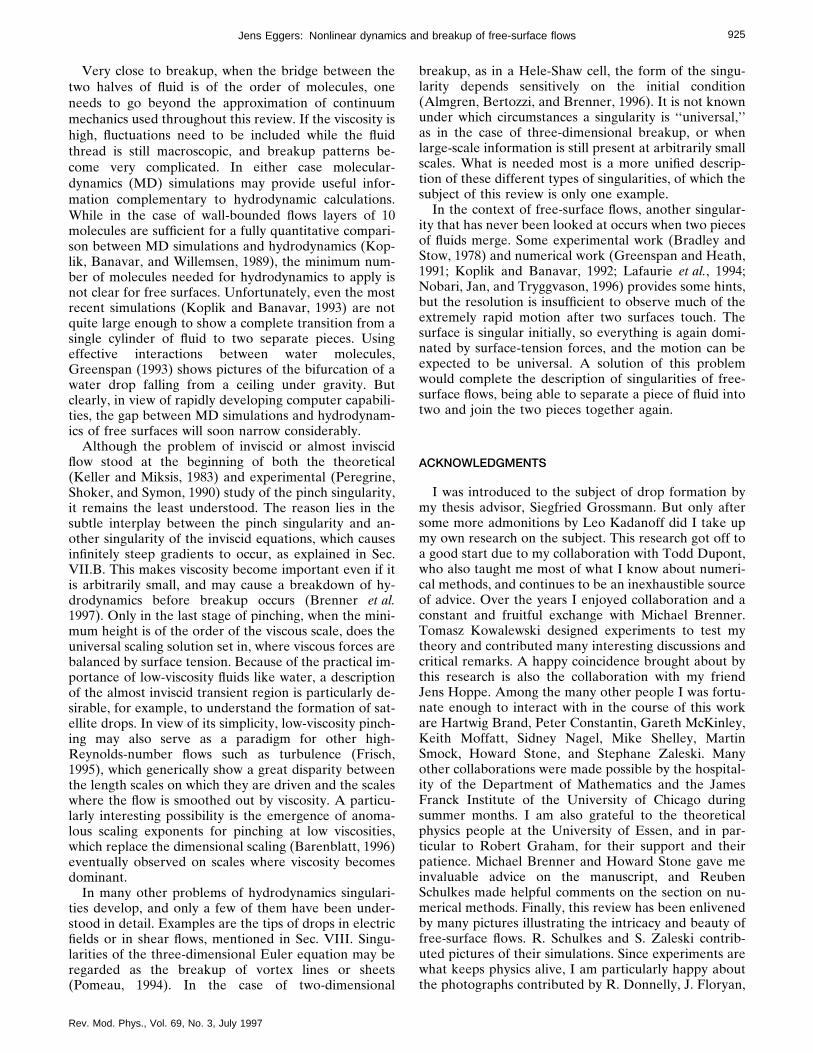
925Jens Eggers: Nonlinear dynamics and breakup of free-surface flows
Very close to breakup, when the bridge between thetwo halves of fluid is of the order of molecules, oneneeds to go beyond the approximation of continuummechanics used throughout this review. If the viscosity ishigh, fluctuations need to be included while the fluidthread is still macroscopic, and breakup patterns be-come very complicated. In either case molecular-dynamics (MD) simulations may provide useful infor-mation complementary to hydrodynamic calculations.While in the case of wall-bounded flows layers of 10molecules are sufficient for a fully quantitative compari-son between MD simulations and hydrodynamics (Kop-lik, Banavar, and Willemsen, 1989), the minimum num-ber of molecules needed for hydrodynamics to apply isnot clear for free surfaces. Unfortunately, even the mostrecent simulations (Koplik and Banavar, 1993) are notquite large enough to show a complete transition from asingle cylinder of fluid to two separate pieces. Usingeffective interactions between water molecules,Greenspan (1993) shows pictures of the bifurcation of awater drop falling from a ceiling under gravity. Butclearly, in view of rapidly developing computer capabili-ties, the gap between MD simulations and hydrodynam-ics of free surfaces will soon narrow considerably.
Although the problem of inviscid or almost inviscidflow stood at the beginning of both the theoretical(Keller and Miksis, 1983) and experimental (Peregrine,Shoker, and Symon, 1990) study of the pinch singularity,it remains the least understood. The reason lies in thesubtle interplay between the pinch singularity and an-other singularity of the inviscid equations, which causesinfinitely steep gradients to occur, as explained in Sec.VII.B. This makes viscosity become important even if itis arbitrarily small, and may cause a breakdown of hy-drodynamics before breakup occurs (Brenner et al.1997). Only in the last stage of pinching, when the mini-mum height is of the order of the viscous scale, does theuniversal scaling solution set in, where viscous forces arebalanced by surface tension. Because of the practical im-portance of low-viscosity fluids like water, a descriptionof the almost inviscid transient region is particularly de-sirable, for example, to understand the formation of sat-ellite drops. In view of its simplicity, low-viscosity pinch-ing may also serve as a paradigm for other high-Reynolds-number flows such as turbulence (Frisch,1995), which generically show a great disparity betweenthe length scales on which they are driven and the scaleswhere the flow is smoothed out by viscosity. A particu-larly interesting possibility is the emergence of anoma-lous scaling exponents for pinching at low viscosities,which replace the dimensional scaling (Barenblatt, 1996)eventually observed on scales where viscosity becomesdominant.
In many other problems of hydrodynamics singulari-ties develop, and only a few of them have been under-stood in detail. Examples are the tips of drops in electricfields or in shear flows, mentioned in Sec. VIII. Singu-larities of the three-dimensional Euler equation may beregarded as the breakup of vortex lines or sheets(Pomeau, 1994). In the case of two-dimensional
Rev. Mod. Phys., Vol. 69, No. 3, July 1997
breakup, as in a Hele-Shaw cell, the form of the singu-larity depends sensitively on the initial condition(Almgren, Bertozzi, and Brenner, 1996). It is not knownunder which circumstances a singularity is ‘‘universal,’’as in the case of three-dimensional breakup, or whenlarge-scale information is still present at arbitrarily smallscales. What is needed most is a more unified descrip-tion of these different types of singularities, of which thesubject of this review is only one example.
In the context of free-surface flows, another singular-ity that has never been looked at occurs when two piecesof fluids merge. Some experimental work (Bradley andStow, 1978) and numerical work (Greenspan and Heath,1991; Koplik and Banavar, 1992; Lafaurie et al., 1994;Nobari, Jan, and Tryggvason, 1996) provides some hints,but the resolution is insufficient to observe much of theextremely rapid motion after two surfaces touch. Thesurface is singular initially, so everything is again domi-nated by surface-tension forces, and the motion can beexpected to be universal. A solution of this problemwould complete the description of singularities of free-surface flows, being able to separate a piece of fluid intotwo and join the two pieces together again.
ACKNOWLEDGMENTS
I was introduced to the subject of drop formation bymy thesis advisor, Siegfried Grossmann. But only aftersome more admonitions by Leo Kadanoff did I take upmy own research on the subject. This research got off toa good start due to my collaboration with Todd Dupont,who also taught me most of what I know about numeri-cal methods, and continues to be an inexhaustible sourceof advice. Over the years I enjoyed collaboration and aconstant and fruitful exchange with Michael Brenner.Tomasz Kowalewski designed experiments to test mytheory and contributed many interesting discussions andcritical remarks. A happy coincidence brought about bythis research is also the collaboration with my friendJens Hoppe. Among the many other people I was fortu-nate enough to interact with in the course of this workare Hartwig Brand, Peter Constantin, Gareth McKinley,Keith Moffatt, Sidney Nagel, Mike Shelley, MartinSmock, Howard Stone, and Stephane Zaleski. Manyother collaborations were made possible by the hospital-ity of the Department of Mathematics and the JamesFranck Institute of the University of Chicago duringsummer months. I am also grateful to the theoreticalphysics people at the University of Essen, and in par-ticular to Robert Graham, for their support and theirpatience. Michael Brenner and Howard Stone gave meinvaluable advice on the manuscript, and ReubenSchulkes made helpful comments on the section on nu-merical methods. Finally, this review has been enlivenedby many pictures illustrating the intricacy and beauty offree-surface flows. R. Schulkes and S. Zaleski contrib-uted pictures of their simulations. Since experiments arewhat keeps physics alive, I am particularly happy aboutthe photographs contributed by R. Donnelly, J. Floryan,
926 Jens Eggers: Nonlinear dynamics and breakup of free-surface flows
G. Jameson, T. Kowalewski, G. Leal, H. Leonhard, S.Nagel, J. Ottino, S. Spiegelberg, H. Stone, and A. Yarin.
REFERENCES
Acrivos, A., and T. S. Lo, 1978, J. Fluid Mech. 86, 641.Aguirre-de-Carcer, I., and J. Fernandez de la Mora, 1995, J.
Colloid Interface Sci. 171, 512.Almgren, R., A. Bertozzi, and M. P. Brenner, 1996, Phys. Flu-
ids 8, 1356.Altschuler, S., S. B. Angenent, and Y. Giga, 1995, J. Geom.
Anal. 5, 293.Amit, D. J., 1978, Field Theory, The Renormalization Group
and Critical Phenomena (McGraw-Hill, New York).Ashgriz, N., and F. Mashayek, 1995, J. Fluid Mech. 291, 163.Bacri, J. C., and D. Salin, 1982, J. Phys. (France) Lett. 43,
L649.Bailey, A. G., 1988, Electrostatic Spraying of Liquids (Wiley,
New York).Baker, G. R., D. I. Meiron, and S. A. Orszag, 1980, Phys. Flu-
ids 23, 1485.Barenblatt, G. I., 1996, Scaling, Self-Similarity, and Intermedi-
ate Asymptotics (Cambridge University, Cambridge, En-gland).
Barthes-Biesel, D., and A. Acrivos, 1973, J. Fluid Mech. 61, 1.Bar-Ziv, R., and E. Moses, 1994, Phys. Rev. Lett. 73, 1392.Bechtel, S. E., K. Bolinger, G. Cao, and M. G. Forest, 1995,
SIAM (Soc. Ind. Appl. Math.) J. Appl. Math. 55, 58.Bechtel, S. E., C. D. Carlson, and M. G. Forest, 1995, Phys.
Fluids 7, 2957.Bechtel, S. E., M. G. Forest, and K. J. Lin, 1992, SAACM 2,
59.Becker, E., W. J. Hiller, and T. A. Kowalewski, 1991, J. Fluid
Mech. 231, 189.Becker, E., W. J. Hiller, and T. A. Kowalewski, 1994, J. Fluid
Mech. 258, 191.Bender, C. M., and S. A. Orszag, 1978, Advanced Mathemati-
cal Methods for Scientists and Engineers (McGraw-Hill, NewYork).
Bensimon, D., L. P. Kadanoff, S. Liang, B. I. Shraiman, and C.Tang, 1986, Rev. Mod. Phys. 58, 977.
Bentley, B. J., and L. G. Leal, 1986a, J. Fluid Mech. 167, 219.Bentley, B. J., and L. G. Leal, 1986b, J. Fluid Mech. 167, 241.Berger S. A., 1988, SIAM (Soc. Ind. Appl. Math.) J. Appl.
Math. 48, 973.Bertozzi, A. L., M. P. Brenner, T. F. Dupont, and L. P.
Kadanoff, 1994, in Trends and Perspectives in Applied Math-ematics, Applied Mathematics Series, Vol. 100, edited by L.Sirovich (Springer, New York), p. 155.
Bidone, G., 1823, Mem. Accad. Sci. di Torino 27, 83.Bird, R. B., R. C. Armstrong, and O. Hassager, 1987, Dynam-
ics of Polymeric Liquids, Volume I: Fluid Mechanics; VolumeII: Kinetic Theory (Wiley, New York).
Bogy, D. B., 1978a, J. Appl. Mech. 45, 469.Bogy, D. B., 1978b, Phys. Fluids 21, 190.Bogy, D. B., 1979a, Phys. Fluids 22, 224; 23, 421.Bogy, D. B., 1979b, Annu. Rev. Fluid Mech. 11, 207.Bogy, D. B., S. J. Shine, and F. E. Talke, 1980, J. Comput.
Phys. 38, 294.Bohr, N., 1909, Philos. Trans. R. Soc. London, Ser. A 209, 281.Bousfield, D. W., R. Keunigs, G. Marrucci, and M. M. Denn,
1986, J. Non-Newton. Fluid Mech. 21, 79.
Rev. Mod. Phys., Vol. 69, No. 3, July 1997
Bradley, S. G., and C. D. Stow, 1978, Philos. Trans. R. Soc.London, Ser. A 287, 635.
Brenner, M. P., 1997, private communication.Brenner, M. P., J. Eggers, K. Joseph, S. R. Nagel, and X. D.
Shi, 1997, Phys. Fluids 9, 1573.Brenner, M. P., J. R. Lister, and H. A. Stone, 1996, Phys. Flu-
ids 8, 2827.Brenner, M. P., X. D. Shi, and S. R. Nagel, 1994, Phys. Rev.
Lett. 73, 3391.Brosa, U., S. Grossmann, and A. Muller, 1990, Phys. Rep. 197,
167.Buckmaster, J. D., 1972, J. Fluid Mech. 55, 385.Chandrasekhar, S., 1961, Hydrodynamic and Hydromagnetic
Stability (Oxford University, New York/London). Reprinted1981 (Dover, New York).
Chaudhary, K. C., and T. Maxworthy, 1980a, J. Fluid Mech. 96,275.
Chaudhary, K. C., and T. Maxworthy, 1980b, J. Fluid Mech. 96,287.
Chaudhary, K. C., and L. G. Redekopp, 1980, J. Fluid Mech.96, 257.
Cline, H. E., and T. R. Anthony, 1978, J. Appl. Phys. 49, 3203.Constantin, P., 1992, private communication.Constantin, P., T. F. Dupont, R. E. Goldstein, L. P. Kadanoff,
M. J. Shelley, and S. M. Zhou, 1993, Phys. Rev. E 47, 4169.Cowley, M. D., and R. E. Rosensweig, 1967, J. Fluid Mech. 30,
671.Crane, L. S., S. Birch, and P. O. McCormack, 1964, Brit. J.
Appl. Phys. 15, 743.Dafermos C. M., 1987, SIAM (Soc. Ind. Appl. Math.) J. Math.
Anal. 18, 409.Da-Riva, I., 1981, in Applications of Space Development,
XXXI International Astronautical Congress, edited by L. G.Napolitano (Pergamon, New York), p. 69.
de Bruijn, R. A., 1993, Chem. Eng. Sci. 48, 277.de Laplace, P. S., 1805, Mechanique Celeste, Supplement au
Xieme Livre (Courcier, Paris).Deckelnick, K., 1997, ‘‘Weak Solutions of the Curve Shorten-
ing Flow,’’ Calc. Var., in press.Dewynne, J. N., P. D. Howell, and P. Wilmott, 1994, Q. J.
Mech. Appl. Math. 47, 541.Dold, J. W., 1992, J. Comput. Phys. 103, 90.Dommermuth, D. G., and D. K. P. Yue, 1987, J. Fluid Mech.
178, 195.Donnelly, R. J., and W. Glaberson, 1966, Proc. R. Soc. Lon-
don, Ser. A 290, 547.Dupont, T. F., 1993, private communication.Edgerton, H. E., 1977, in Stopping Time: The Photographs of
Harold Edgerton, edited by Gus Kayafas (Abrams, NewYork, 1987).
Edgerton, H. E., E. A. Hauser, and W. B. Tucker, 1937, J.Phys. Chem. 41, 1029.
Eggers, J., 1993, Phys. Rev. Lett. 71, 3458.Eggers, J., 1995a, Phys. Fluids 7, 941.Eggers, J., 1995b, ‘‘Nonlinear stability in one-dimensional
models,’’ unpublished.Eggers, J., 1995c, ‘‘Satellite formation in one-dimensional
models,’’ unpublished.Eggers, J., 1997, ‘‘Singularities in droplet pinching without vis-
cosity,’’ Los Alamos preprint No. chao-dyn/9705006.Eggers, J., and T. F. Dupont, 1994, J. Fluid Mech. 262, 205.Entov, V. M., and A. L. Yarin, 1984, J. Fluid Mech. 140, 91.

927Jens Eggers: Nonlinear dynamics and breakup of free-surface flows
Fenn, J. B., M. Mann, C. K. Meng, S. F. Wong, and C. M.Whitehouse, 1989, Science 246, 64.
Fernandez de la Mora, J., and I. G. Loscertales, 1994, J. FluidMech. 260, 155.
Forest, M. G., and Q. Wang, 1990, J. Theor. Comp. Fluid Dyn.2, 1.
Forest, M. G., and Q. Wang, 1994, SIAM (Soc. Ind. Appl.Math.) J. Appl. Math. 54, 996.
Frankel, I., and D. Weihs, 1985, J. Fluid Mech. 155, 289.Frisch, U., 1995, Turbulence (Cambridge University, Cam-
bridge, England).Fromm, J. E., 1984, IBM J. Res. Dev. 28, 322.Gabovich, M. D., 1983, Usp. Fiz. Nauk 140, 137 [Sov. Phys.
Usp. 26, 447 (1983)].Garcıa, F. J., and A. Castellanos, 1994, Phys. Fluids 6, 2676.Gaudet, S., G. H. McKinley, and H. A. Stone, 1996, Phys.
Fluids 8, 2568.Giesekus, H., 1982, J. Non-Newton. Fluid Mech. 11, 69.Giga, Y., and R. V. Kohn, 1989, Commun. Pure Appl. Math.
42, 845.Gillette, R. D., and D. C. Dyson, 1971, Chem. Eng. 2, 44.Goedde, E. F., and M. C. Yuen, 1970, J. Fluid Mech. 40, 495.Goldin, M., J. Yerushalmi, R. Pfeffer, and R. Shinnar, 1969, J.
Fluid Mech. 38, 689.Gradshteyn, I. S., and I. M. Ryzhik, 1980, Table of Integrals,
Series, and Products (Academic, New York).Grauer, R., and T. C. Sideris, 1991, Phys. Rev. Lett. 67, 3511.Green, A. E., 1976, Int. J. Eng. Sci. 14, 49.Green, A. E., and N. Laws, 1966, Proc. R. Soc. London, Ser. A
293, 145.Greenspan, D., 1993, System Analysis Modelling Simulation,
Vol. 11 (Gordon and Breach, New York), p. 87.Greenspan, D., and L. F. Heath, 1991, J. Phys. D 24, 2121.Grossmann, S., and A. Muller, 1984, Z. Phys. B 57, 161.Grundy, R. E., 1983, IMA J. Appl. Math. 30, 209.Grundy, R. E., and V. A. Bell, 1993, Proc. R. Soc. London,
Ser. A 441, 641.Guderley, A., 1942, Luftfahrt-Forsch. 19, 302.Gueyffier, D., and S. Zaleski, 1997, ‘‘Simulations of colliding
drops with SURFER,’’ unpublished.Guthrie, F., 1864, Proc. R. Soc. London 13, 444.Haenlein, A., 1931, Forsch. Geb. Ingenieurwes. 2, 139.Hagen, G., 1849, Bericht uber die zur Bekanntmachung
geeigneten Verhandlungen der preussischen Akademie derWissenschaften (Akademie-Verlag, Berlin), p. 281.
Happel, J., and H. Brenner, 1983, Low Reynolds Number Hy-drodynamics (Nijhoff, The Hague).
Harkins, W. D., and F. E. Brown, 1919, J. Am. Chem. Soc. 41,499.
Harris, M. T., and O. A. Basaran, 1993, J. Colloid InterfaceSci. 161, 389.
Hauser, E. A., H. E. Edgerton, B. M. Holt, and J. T. Cox, Jr.,1936, J. Phys. Chem. 40, 973.
Hayati, I., A. I. Bailey, and T. F. Tadros, 1986, Nature (Lon-don) 319, 41.
Hayati, I., A. I. Bailey, and T. F. Tadros, 1987, J. Colloid In-terface Sci. 117, 205.
Henderson, D. M., W. G. Pritchard, and L. B. Smolka, 1997,‘‘On the pinch-off of a pendant drop of a viscous fluid,’’Pennsylvania, State University preprint.
Hiller, W. J., and T. A. Kowalewski, 1989, Opt. Eng. (Belling-ham) 28, 197.
Hinch, E. J., 1977, Phys. Fluids 20, S22.
Rev. Mod. Phys., Vol. 69, No. 3, July 1997
Hinch, E. J., and A. Acrivos, 1979, J. Fluid Mech. 91, 401.Hinch, E. J., and A. Acrivos, 1980, J. Fluid Mech. 98, 305.Hirt, C. W., and B. D. Nichols, 1981, J. Comput. Phys. 39, 201.Hoppe, J., 1992, Lectures on Integrable Systems (Springer,
Berlin).Hoppe, J., 1995, private communication.Huisken, G., 1991, J. Diff. Geom. 31, 285.Inculet, I. I., and J. M. Floryan, 1990, Int. J. Microgr. Res.
Appl. 3, 148.Jackson, J. D., 1975, Classical Electrodynamics, 2nd edition
(Wiley, New York).Jeong, J.-T., and H. K. Moffatt, 1992, J. Fluid Mech. 241, 1.Johnson, G. R., E. Marschall, and J. H. Esdorn, 1985, Rev. Sci.
Instrum. 56, 264.Johnson, M., R. D. Kamm, L. W. Ho, A. Shapiro, and T. J.
Pedley, 1991, J. Fluid Mech. 233, 141.Joseph, D. D., J. Nelson, M. Renardy, and Y. Renardy, 1991, J.
Fluid Mech. 223, 383.Keller, J. B., 1983, Phys. Fluids 26, 3451.Keller, J. B., A. King, and L. Ting, 1995, Phys. Fluids 7, 226.Keller, J. B., and M. J. Miksis, 1983, SIAM (Soc. Ind. Appl.
Math.) J. Appl. Math. 43, 268.Keller, J. B., S. I. Rubinow, and Y. O. Tu, 1973, Phys. Fluids
16, 2052.Kessler, D. A., J. Koplik, and H. Levine, 1988, Adv. Phys. 37,
255.Keunings, R., 1986, J. Comput. Phys. 62, 199.Koplik, J., and J. R. Banavar, 1992, Science 257, 1664.Koplik, J., and J. R. Banavar, 1993, Phys. Fluids A 5, 521.Koplik, J., J. R. Banavar, and J. F. Willemsen, 1989, Phys.
Fluids A 1, 781.Kowalewski, T. A., 1996, Fluid Dyn. Res. 17, 121.Ladyzhenskaya, O., 1969, The Mathematical Theory of Viscous
Incompressible Flow, 2nd ed. (Gordon and Breach, NewYork).
Lafaurie, B., C. Nardone, R. Scardovelli, S. Zaleski, and G.Zanetti, 1994, J. Comput. Phys. 113, 134.
Lafrance, P., 1975, Phys. Fluids 18, 428.Landau, L. D., and E. M. Lifshitz, 1984a, Fluid Mechanics
(Pergamon, Oxford).Landau, L. D., and E. M. Lifshitz, 1984b, Electrodynamics of
Continuous Media (Pergamon, Oxford).Lee, H. C., 1974, IBM J. Res. Dev. 18, 364.Leib, S. J., and M. E. Goldstein, 1986, J. Fluid Mech. 168, 479.Leonhard, H., 1996, ‘‘Experiments on tipstreaming,’’ unpub-
lished.Li, H., T. C. Halsey, and A. Lobkovsky, 1994, Europhys. Lett.
27, 575.Lin, S. P., and D. J. Kang, 1987, Phys. Fluids 30, 2000.Lin, S. P., and R. D. Webb, 1994, Phys. Fluids 6, 2671.Lister, J. R., and H. A. Stone, 1996, J. Fluid Mech. 317, 275.Lister, J. R., H. Stone, and M. P. Brenner, 1997 unpublished.Longuet-Higgins, M. S., and E. D. Cokelet, 1976, Proc. R. Soc.
London, Ser. A 350, 1.Magnus, G., 1855, Ann. Phys. Chem. 95, 1.Majda, A. J., 1991, SIAM (Soc. Ind. Appl. Math.) Rev. 39, 349.Mansour, N. N., and T. S. Lundgren, 1990, Phys. Fluids A 2,
1141.Manwell, A. R., 1971, The Hodograph Equations (Hafner,
Darien, Connecticut).Mariotte, E., 1686, Traite du mouvement des eaux et des autres
corps fluides (E. Michallet, Paris).

928 Jens Eggers: Nonlinear dynamics and breakup of free-surface flows
Marschall, E., 1985, Verh. Deutsch. Ingen. Forschungsheft 632,13.
Matovitch, M. A., and J. R. A. Pearson, 1969, Ind. Eng. Chem.Fundamentals 8, 512.
Maxwell, J. C., 1875, in Encyclopedia Britannica, 9th edition.Reprinted 1965 in The Scientific Papers of James Clerk Max-well, edited by W. D. Niven (Dover, New York), Vol. II, p.541.
McCarthy, M. J., and N. A. Malloy, 1974, Chem. Eng. J. 7, 1.Merle, F., 1992, Commun. Pure Appl. Math. 45, 203.Meseguer, J., 1983, J. Fluid Mech. 130, 123.Meseguer, J., and A. Sanz, 1985, J. Fluid Mech. 153, 83.Meseguer, J., A. Sanz, and J. Lopez, 1986, J. Cryst. Growth 78,
325.Mestel, A. J., 1994, J. Fluid Mech. 274, 93.Michael, D. H., and P. G. Williams, 1976, Proc. R. Soc. Lon-
don, Ser. A 351, 117.Middleman, S., 1995, Modeling Axisymmetric Flows (Aca-
demic, New York).Mikami, T., R. G. Cox, and S. G. Mason, 1975, J. Multiphase
Flow 2, 113.Miksis, M. J., 1981, Phys. Fluids 24, 1967.Moffatt, H. K., 1995, private communication.Moore, D. W., 1983, IMA J. Appl. Math. 31, 1.Muller, A., and S. Grossmann, 1985, Z. Naturforsch. Teil A 40,
968.Nayfeh, A. H., 1970, Phys. Fluids 14, 841.Nobari, M. R., Y.-J. Jan, and G. Tryggvason, 1996, Phys. Fluids
8, 29.Og uz, H. N., and A. Prosperetti, 1990, J. Fluid Mech. 219, 143.Olver, P. J., and Y. Nutku, 1988, J. Math. Phys. (N.Y.) 29,
1610.Pantano, C., A. M. Gan an-Calvo, and A. Barrero, 1994, J.
Aerosol Sci. 25, 1065.Papageorgiou, D. T., 1995, Phys. Fluids 7, 1529.Pearson, J. R. A., and M. A. Matovitch, 1969, Ind. Eng. Chem.
Fundamentals 8, 605.Pelekasis, N. A., J. A. Tsamopoulos, and G. D. Manolis, 1992,
J. Comput. Phys. 101, 231.Perales, J. M., and J. Meseguer, 1992, Phys. Fluids 4, 1110.Peregrine, D. H., 1972, in Waves on Beaches, edited by R. E.
Meyer (Academic, New York), p. 95.Peregrine, D. H., G. Shoker, and A. Symon, 1990, J. Fluid
Mech. 212, 25.Pimbley, W. T., 1976, IBM J. Res. Dev. 20, 148.Pimbley, W. T., and H. C. Lee, 1977, IBM J. Res. Dev. 21, 21.Plateau, J., 1843, Acad. Sci. Bruxelles Mem. 16, 3.Plateau, J., 1849, Acad. Sci. Bruxelles Mem. 23, 5.Plateau, J., 1857, Acad. Sci. Bruxelles Mem. 30, 3.Plateau, J., 1873, Statique Experimentale et Theoretique des
Liquides Soumis aux Seules Forces Moleculaires (GauthierVillars, Paris), Vol. II, p. 319.
Pomeau, Y., 1994, C. R. Acad. Sci. Paris 318, 865.Press, W. H., S. A. Teukolski, W. T. Vetterling, and B. P.
Flannery, 1992, Numerical Recipes, 2nd ed. (Cambridge Uni-versity, Cambridge, England).
Pumir, A., and E. D. Siggia, 1992, Phys. Fluids A 4, 1472.Rallison, J. M., and A. Acrivos, 1978, J. Fluid Mech. 89, 191.Rallison, J. M., 1984, Annu. Rev. Fluid Mech. 16, 45.Rayleigh, Lord, J. W. S., 1879a, Proc. London Math. Soc. 10, 4
(appeared in the volume of 1878).Rayleigh, Lord, J. W. S., 1879b, Proc. R. Soc. London, Ser. A
29, 94.
Rev. Mod. Phys., Vol. 69, No. 3, July 1997
Rayleigh, Lord, J. W. S., 1882, Proc. R. Soc. London, Ser. A34, 130.
Rayleigh, Lord, J. W. S., 1891, Nature (London) 44, 249.Rayleigh, Lord, J. W. S., 1892, Philos. Mag. 34, 145.Rayleigh, Lord, J. W. S., 1896, The Theory of Sound (Mac-
millan, London). Reprinted 1945, 2nd ed. (Dover, NewYork), Vol. II, p. 351.
Rayleigh, Lord, J. W. S., 1899, Philos. Mag. 48, 321.Razumovski�, N. A., 1993, Zh. Tekh. Fiz. 63, 26 [Tech. Phys.
38, 752 (1993)].Rehage, H., and H. Hoffmann, 1991, Mol. Phys. 74, 933.Renardy, M., 1982, SIAM (Soc. Ind. Appl. Math.) J. Math.
Anal. 13, 226.Renardy, M., 1994, J. Non-Newton. Fluid Mech. 51, 97.Renardy, M., 1995, J. Non-Newton. Fluid Mech. 59, 267.Reynolds, O., 1886, Philos. Trans. R. Soc. London 177, 157.Richards, J. R., A. M. Lenhoff, and A. N. Beris, 1994, Phys.
Fluids 6, 2640.Rutland, D. F., and G. J. Jameson, 1970, Chem. Eng. Sci. 25,
1689.Rutland, D. F., and G. J. Jameson, 1971, J. Fluid Mech. 46, 267.Savart, F., 1833, Annal. Chim. 53, 337, plates in Vol. 54.Schneider, J. M., N. R. Lindblatt, C. D. Hendricks, Jr., and J.
M. Crowley, 1967, J. Appl. Phys. 38, 2599.Schulkes, R. M. S. M., 1993, Phys. Fluids A 5, 2121.Schulkes, R. M. S. M., 1994a, J. Fluid Mech. 261, 223.Schulkes, R. M. S. M., 1994b, J. Fluid Mech. 278, 83.Schultz, W. W., and S. H. Davis, 1982, J. Rheol. 26, 331.Sedov, L. I., 1946, Prikl. Mat. Mekh. 10, 241.Sherwood, J. D., 1981, Math. Proc. Camb. Philos. Soc. 90, 529.Sherwood, J. D., 1984, J. Fluid Mech. 144, 281.Sherwood, J. D., 1988, J. Fluid Mech. 188, 133.Sherwood, J. D., 1991, J. Phys. A 24, 4047.Shi, X. D., M. P. Brenner, and S. R. Nagel, 1994, Science 265,
157.Shield, T. W., D. B. Bogy, and F. E. Talke, 1986, J. Comput.
Phys. 67, 327.Shipman, R. W. G., M. M. Denn, and R. Keunings, 1991, J.
Non-Newton. Fluid Mech. 40, 281.Shokoohi, F., and H. G. Elrod, 1987, J. Comput. Phys. 71, 324.Shokoohi, F., and H. G. Elrod, 1990, J. Comput. Phys. 89, 483.Spangler, C. A., J. H. Hilbing, and S. D. Heister, 1995, Phys.
Fluids 7, 964.Spiegelberg, S. H., D. C. Ables, and G. H. McKinley, 1996, J.
Non-Newton. Fluid Mech. 64, 229.Spiegelberg, S. H., S. Gaudet, and G. H. McKinley, 1994, in
Extensional Deformation of Non-Newtonian Materials: Liq-uid Bridge Studies, 2nd Microgravity Fluid Physics Confer-ence, Cleveland, Ohio, Vol. CP-3276 (U.S. Govt. Printing Of-fice 1994-553-454), p. 311.
Spiegelberg, S. H., and G. H. McKinley, 1996, J. Non-Newton.Fluid Mech. 67, 49.
Sridhar, T. S., V. Tirtaatmadja, D. A. Nguyen, and R. K.Gupta, 1991, J. Non-Newton. Fluid Mech. 40, 271.
Stone, H. A., 1994, Annu. Rev. Fluid Mech. 26, 65.Stone, H. A., B. J. Bentley, and L. G. Leal, 1986, J. Fluid
Mech. 173, 131.Stone, H. A., and M. P. Brenner, 1996, J. Fluid Mech. 318, 373.Stone, H. A., and L. G. Leal, 1989a, J. Fluid Mech. 198, 399.Stone, H. A., and L. G. Leal, 1989b, J. Fluid Mech. 206, 223.Stone, H. A., J. R. Lister, and M. P. Brenner, 1997, ‘‘Drops
with conical ends in electric and magnetic fields,’’ HarvardUniversity preprint.

929Jens Eggers: Nonlinear dynamics and breakup of free-surface flows
Tate, T., 1864, Philos. Mag. 27, 176.Taub, H. H., 1976, Phys. Fluids 19, 1124.Taylor, G. I., 1932, Proc. R. Soc. London, Ser. A 138, 41.Taylor, G. I., 1934, Proc. R. Soc. London, Ser. A 146, 501.Taylor, G. I., 1964, Proc. R. Soc. London, Ser. A 280, 383.Taylor, G. I., 1966, in Proceedings of 11th International Con-
gress of Applied Mechanics, Munich, 1964 (Springer, Heidel-berg). Reprinted 1971 in The Scientific Papers of Sir GeoffryIngram Taylor, edited by G. K. Batchelor (Cambridge Uni-versity, Cambridge, England), Vol. IV.
Taylor, G. I., 1969, Proc. R. Soc. London, Ser. A 313, 453.Ting, L., and J. B. Keller, 1990, SIAM (Soc. Ind. Appl. Math.)
J. Appl. Math. 50, 1533.Tjahjadi, M., and J. M. Ottino, 1991, J. Fluid Mech. 232, 191.Tjahjadi, M., H. A. Stone, and J. M. Ottino, 1992, J. Fluid
Mech. 243, 297.Tomotika, S., 1935, Proc. R. Soc. London, Ser. A 150, 322.Tomotika, S., 1936, Proc. R. Soc. London, Ser. A 153, 302.Torpey, P. A., 1988, Phys. Fluids A 1, 661.Trouton, F. T., 1906, Proc. R. Soc. London, Ser. A 77, 426.Tsai, W.-T., and D. K. P. Yue, 1996, Annu. Rev. Fluid Mech.
28, 249.Tur, A. V., and V. V. Yanovsky, 1993, J. Fluid Mech. 248, 67.Van Dyke, M., 1975, Perturbation Methods in Fluid Mechanics,
second Ed. (Parabolic, Stanford, California).Vassallo, P., and N. Ashgriz, 1991, Proc. R. Soc. London, Ser.
A 433, 269.
Rev. Mod. Phys., Vol. 69, No. 3, July 1997
Walzel, P., 1988, ‘‘Spraying and Atomizing of Liquids,’’ in Ul-lmann’s Encyclopedia of Industrial Chemistry, 5th Ed., Vol.B2 (VCH, Weinheim).
Wang, D. P., 1968, J. Fluid Mech. 34, 299.Weast, R. C., 1978, Ed., Handbook of Chemistry and Physics
(CRC Press, Cleveland, Ohio).Weber, C., 1931, Z. Angew. Math. Mech. 11, 136.Wilson, S. D. R., 1988, J. Fluid Mech. 190, 561.Worthington, A. M., 1881, Proc. R. Soc. London, Ser. A 32,
362.Worthington, A. M., 1908, A Study of Splashes (Longmans,
London).Yang, H. Q., 1992, Phys. Fluids A 4, 681.Yarin, A. L., 1993, Free Liquid Jets and Films: Hydrodynamics
and Rheology (Wiley, New York).Yarin, A. L., and D. A. Weiss, 1995, J. Fluid Mech. 283, 141.Young, T., 1805, Philos. Trans. R. Soc. London 95, 65.Youngren, G. K., and A. Acrivos, 1975, J. Fluid Mech. 69, 377.Yuen, M.-C., 1968, J. Fluid Mech. 33, 151.Zeleny, J., 1914, Phys. Rev. 3, 69.Zeleny, J., 1915, Proc. Camb. Philos. Soc. 18, 71.Zeleny, J., 1917, Phys. Rev. 10, 1.Zhang, X., and O. A. Basaran, 1995, Phys. Fluids 7, 1184.Zhang, X., R. S. Padgett, and O. A. Basaran, 1996, J. Fluid
Mech. 329, 207.