Nonlinear chaotic model for predicting storm surges · Nonlinear chaotic model for predicting storm...

Nonlin. Processes Geophys., 17, 405–420, 2010www.nonlin-processes-geophys.net/17/405/2010/doi:10.5194/npg-17-405-2010© Author(s) 2010. CC Attribution 3.0 License.

Nonlinear Processesin Geophysics

Nonlinear chaotic model for predicting storm surges

M. Siek1 and D. P. Solomatine1,2

1Department of Hydroinformatics and Knowledge Management, UNESCO-IHE Institute for Water Education,Delft, The Netherlands2Water Resources Section, Delft University of Technology, The Netherlands

Received: 29 November 2009 – Revised: 27 August 2010 – Accepted: 31 August 2010 – Published: 6 September 2010

Abstract. This paper addresses the use of the methodsof nonlinear dynamics and chaos theory for building apredictive chaotic model from time series. The chaotic modelpredictions are made by the adaptive local models based onthe dynamical neighbors found in the reconstructed phasespace of the observables. We implemented the univariateand multivariate chaotic models with direct and multi-stepsprediction techniques and optimized these models using anexhaustive search method. The built models were testedfor predicting storm surge dynamics for different stormyconditions in the North Sea, and are compared to neuralnetwork models. The results show that the chaotic modelscan generally provide reliable and accurate short-term stormsurge predictions.

1 Introduction

Storm surge is a meteorologically forced long wave motionwhich is pushed toward the shore. It is generated by acombination of meteorological forces of the wind frictionand low air pressure due to a storm (Gonnert et al., 2001), andoscillates in the period range of a few minutes to a few days.In the ocean, local wind waves can add to the water level, andthe storm surge can be amplified (or reduced) by interferencewith the strictly regular astronomical tides. Extreme coastalfloods can be related to extreme storms, like cyclones orhurricanes which attack the open coast. In some coastalareas, such floods can be generated by unusual sequencesof wind set-up and air pressure variations. In addition, winddriven waves can be superimposed on the storm tide. Thisrise in sea level can cause severe flooding in coastal areas,particularly when the storm tide coincides with the high tides(Battjes et al., 2002).

Correspondence to:M. Siek([email protected])

Astronomical tides generally have the large contributionto the ocean water level variations in open oceans andmany well-exposed coasts. Traditionally, the analysis ofwater levels usually employs linear methods that decomposesea levels into tides and other (usually meteorological)components. The amplitudes and phases of the tidalconstituents driven by the astronomical motion of the Earth,Moon and Sun (with known periods) can be estimated byusing Fourier analysis, response analysis or linear regressionmethods. In particular, the weakly nonlinear shallow waterwaves can be characterized by the Korteweg-de Vries (KdV)equation (Korteweg and de Vries, 1895) which is an exactsolvable partial differential equation.Zabusky and Kruskal(1965) found that the KdV equation can be obtained in thecontinuum limit of the Fermi-Pasta-Ulam Experiment (Fermiet al., 1955). They showed that the solitary wave solutionshad behavior similar to the superposition principle, despitethe fact that the waves themselves were highly nonlinear.In real applications, however, the water level dynamicsin coastal and estuarial swallow-water areas, such as theDutch coast, may differ significantly from the astronomicalestimated constituents (superposition principle) – due to thenonlinear effects that include meteorological forcing, tidal-current interactions, tidal deformations due to the complextopography and river discharges (Prandle et al., 1978).

Coastal floods due to storm surges can be predictedwith an accuracy that depends on the accuracy of themeteorological forecasts. An appropriate numerical weathermodel can predict the motion of atmospheric depression witha satisfactory accuracy in a range of several days. The windand air surface pressure fields predicted by this model can beutilized as some driving forces of the sea motion in a shallowwater model allowing for storm surge predictions. Somerecent updates on the operational storm surge numericalmodel with data assimilation in the Netherlands have beenstudied byVerlaan et al.(2005).

Published by Copernicus Publications on behalf of the European Geosciences Union and the American Geophysical Union.

http://creativecommons.org/licenses/by/3.0/

406 M. Siek and D. P. Solomatine: Nonlinear chaotic model for predicting storm surges

Nonetheless, the analyses of the risk of coastal floods arenot straightforward, because an observed flood is not a singleindependent event in statistical terms. Rather, the flood isa consequence of a set of different determinants, like tides,wind and air pressure, or of a set of sequences of thesefactors. Both the mean sea level and the flood height willvary along the coast and the risk of coastal flood depends onemergency preparedness planning and the design of coastalfacilities and structures, such as flood embankments. Theocean water level variations due to various determinantsand their complex interactions show long-term persistenceleading to the correlated extreme events (Alexanderssonet al., 1998; Butler et al., 2007).

Complexity of the described phenomena prompts foradequate methods to describe them, and one of them ischaos theory. The most direct link between the conceptof deterministic chaos and the real world is the analysis ofdata (time series) from real systems in terms of the theoryof nonlinear dynamics (Tsonis, 1992; Donner and Barbosa,2008). Note that this approach is, in fact, data-driven,since it is purely based on the analysis of the observationdata. The initial nonlinear analyses of the ocean waterlevels at the Florida coast have been conducted byFrisonet al. (1999). The earlier attempts of the use of chaoticmodel (CM) for storm surge predictions were done bySolomatine et al.(2000), Walton (2005) using univariatelocal models. Velickov (2004) extended the method usingmultivariate chaotic models and showed that it has reliableand accurate short-term predictions. This model has beenfurther improved by applying dimensionality reduction in thephase space (Siek et al., 2008).

This paper presents the use and implementation of thenonlinear dynamics and chaos theory for predicting stormsurges. If compared to our earlier work, we advanced theprocedure of building chaotic model by incorporating severalnew features: using Cao’s method (Cao, 1997) for betterestimation on dynamical invariants; implementing multi-step iterative predictions, applying the neighbors distancecut-off to avoid inclusion of the false dynamical neigh-bors, adding water level variable into multi-variate chaoticmodels, finding the proper number of neighbors usingsensitivity analysis for stormy and non-stormy conditions,and optimizing the chaotic model parameters (time delayand embedding dimension). Furthermore, we compare theprediction performances of the proposed chaotic model withother models, including artificial neural network (ANN)models.

The following sections present the basics of storm surgemodeling, nonlinear dynamics and chaos theory, chaoticmodel prediction, case study, model results and conclusion.

2 Storm surge modeling

Storm surge modeling has advanced significantly over thepast 30 years which turns out to be very essential to anticipatethe occurrence of coastal flooding. Some advances onphysically-based storm surge modeling have been reportedby Bode and Hardy(1997), Battjes et al. (2002) andVerlaan et al.(2005). They include: refining computationalgrids, utilizing more accurate calibration of models withbetter data, using an improved numerical schemes andincorporating data assimilation technique into the model.

Primary links between the nonlinear dynamics and chaostheory, and the storm surge model can be described asfollows. The basis of a physically-based storm surge modelwhich is widely used is the Navier-Stokes shallow waterequations, stating the physical laws of mass and momen-tum conservations (Dronkers, 1964). These equations areinherently nonlinear. The sensitive dependence on the initialand boundary conditions of the dynamical evolution of suchsystems, and the broadband and continuous power spectraare the indicators of deterministic chaos. A mathematicalproof on the existence of chaotic behavior in Navier-Stokesequations and turbulence has been conducted byLi (2004).On other hand,Simonnet et al.(2009) analyzed the presenceof bifurcations in ocean, atmospheric and climate modelsfor understanding the variability of oceanic and atmosphericflows as well as the climate system. As models, chaosdynamical systems show rich and even surprising varietyof dynamical structures and solutions. Most appealing forresearchers and practitioners is the fact that the deterministicchaos provides a prominent explanation for irregular behav-ior and instabilities in dynamical systems (including stormsurges), which are deterministic in nature.

2.1 Study area: the North Sea

The North Sea lies between Norway, Denmark, Germany,the Netherlands, Belgium, France and Great Britain. Itlinks up with the Atlantic Ocean to the north and also thesouthwest, via the English Channel. The total surface area isapproximately 750 000 km2 and the total volume 94 000 km3.The North Sea has a dynamically active regime dominated bystrong tides and frequent passages of mid-latitude synopticweather systems (Droppert et al., 2001). The waters aremostly shallow (depth<150 m) in the region. As tides fromthe deep Atlantic Ocean enter the North West European shelf,they propagate around the coast in the form of long gravitywaves. High tides occur approximately every twelve hours.The main tidal stream enters the North Sea along the Scottishcoast. As a result, the level difference between high tideand low tide is not the same everywhere. The actual tidaldifference depends not only on the positions of the Sun andthe Moon, but also determined by the weather, and primarilyby the wind and surface air pressure. North-westerly stormsare notorious. The rise on any particular occasion dependson the direction, the force and the duration of the storm.

Nonlin. Processes Geophys., 17, 405–420, 2010 www.nonlin-processes-geophys.net/17/405/2010/

M. Siek and D. P. Solomatine: Nonlinear chaotic model for predicting storm surges 407

The extreme storm surges in the North Sea is muchaffected by the role of the North Atlantic Oscillation (NAO)variability (Woodworth et al., 2007). The North Atlanticatmospheric variability is mainly driven by the NAO withan NAO index defined by the difference between normalizedsea-level pressures between the Azores High and IcelandicLow. The periods with large positive index correspond tostrong westerly winds which often strikes the Dutch Coast.

For the Netherlands, the accurate forecasting of stormsurges is very important because of the possible coastalfloods since the large areas of the land lie below sea level.These areas are most densely populated and important forthe economy. Since the disastrous storm of 1953, the dikesand storm surge barriers in the delta area and along theDutch coast have been systematically improved. These dikesand barriers should be operated (i.e. open/close) properlyon the right time to avoid the barrier breaking. For thispurpose, the accurate and reliable predictive models for theocean water level and surge are critically required. Anotherimportant reason for having accurate forecasts of sea levelsis the needs of navigation: the vessels waiting to enter thePort of Rotterdam need these to ensure safe passage throughthe entrance channel since draft of some of them is close tothe depth of the channel.

2.2 Data description

Water level, surge, atmospheric pressure and windspeed/direction data from seven coastal stations along theDutch coast are monitored and provided by the North SeaDirectorate (Directie Noordzee, DNZ). The water levels aresampled at 0.0167 Hz and averaged over period of 10 min.In the data we had at our disposal each time series beginson 1 January 1990 and is available until 31 March 1996,which results in 337 249 continuous samples in total for10 min times series, and 54 768 for the averaged hourlytimes series. Due to the experienced limitations of the usedsoftware to handle extremely large data sets of 10-min data,hourly data is used for all further analysis and building thechaotic model. The surge data is obtained by subtracting theobserved water level with tide (astronomical forces) based onharmonic analysis, formulated as:

surge= water level(observed)− tides (1)

In this paper, we concentrate on predicting the surges atthe Hoek van Holland (HVH) tidal station, which is locatedat the entrance of the Rotterdam harbour. The possibleinclusion of the spatial information from neighboring sta-tions is also investigated for building the multivariate chaoticmodel. We explored the information from Europlatform(EPF) and K13 because in practice the observations fromthese two stations often become reference for the expertjudgement concerning the possible extreme storm surgesat HVH location in relations to the forecasts produced bythe Dutch operational storm surge model (DCSM/WAQUA).

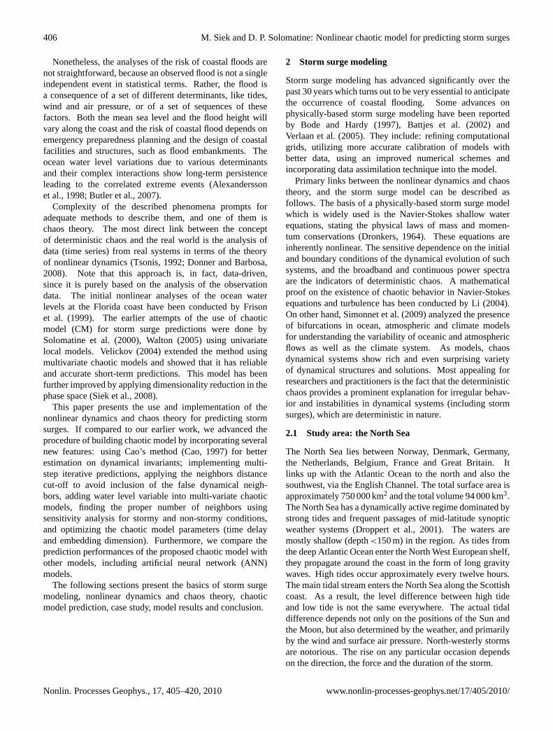
Fig. 1. The North Sea region and the locations of the principalDutch meteorological stations.

Table 1. Data description from tidal stations in the Dutch Coast(1990–1996).

Code Station Water levels SurgesName Max Var. Max Var.

range range(cm) (cm2

×103) (cm) (cm2×103)

EPF Euro platform 438 3.87 357 0.563HVH Hoek v Holland 471 4.63 358 0.708K13 K13 platform 468 2.68 332 0.773

Figure 1 shows the North Sea region and the locations ofthe main tidal stations. Geographically, the EPF stationis closer to the HVH station than the K13 station. Thestorm surge moves from the English Channel (South) to theNorth striking the western part of Dutch Coast, hence theEPF location is a good position in open sea to measure thestorm surges or water levels before they reach to the Port ofRotterdam (Hoek van Holland). This information is requiredfor the preparation before a coastal flood occurs.

Relationship between the long-shore winds, surge, waterlevel, and air pressure difference time series data at HVHlocation is presented in Fig.2. Table 1 illustrates thestatistical description of the data from the three tidal stationsused in this work. In order to evaluate the model performance

www.nonlin-processes-geophys.net/17/405/2010/ Nonlin. Processes Geophys., 17, 405–420, 2010


Table 2. Data separation for surge time series into training, cross-validation and testing data sets for non-stormy and stormy conditions.Cross-validation data sets are used to find the optimal parameters of chaotic model using exhaustive search method.

Date Non-stormy periods Stormy periodsTime Train Test Train Test

Cross-validation data sets

Start 1 Jan 1990 00:00 11 May 1994 15:00 1 Jan 1990 00:00 19 Jan 1994 03:00End 11 May 1994 14:00 28 May 1994 07:00 19 Jan 1994 02:00 4 Feb 1994 19:00

Verification data sets

Start 1 Jan 1990 00:00 1 Jun 1995 23:00 1 Jan 1990 00:00 27 Nov 1994 17:00End 1 Jun 1995 22:00 31 Aug 1995 23:00 27 Nov 1994 16:00 25 Feb 1995 15:00

0 500 1000 1500−50

0

50

Pre

s.di

ff.(m

b)

0 500 1000 1500−50

0

50

Win

d sp

eed

(m/s

)

0 500 1000 1500−200

0

200

Sur

ge (

cm)

0 500 1000 1500−500

0

500

Time samples (hrs)

Wat

er le

vel (

cm)

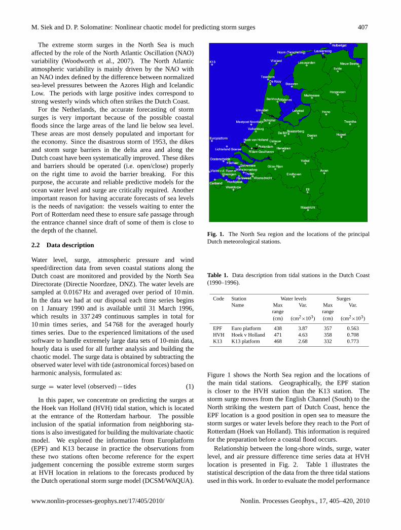
Fig. 2. The relationship between the long-shore winds, surge, waterlevel, and air pressure difference time series at Hoek van Hollandlocation.

for various conditions, the surge data is divided into cross-validation (CV) and verification data sets for non-stormyand stormy conditions as listed in Table2 and depictedon Figs. 3 and 4, respectively. Each of these data setsconsists of training and testing data sets. The cross-validationdata sets are utilized for finding the optimal parametersof chaotic model using exhaustive search method. Afterbeing optimized, the prediction performance of the chaoticmodel was investigated using verification data sets forvarious stormy conditions. The rest of observed time series(1 September 1995 till 31 March 1996) is not used for modelprediction.

Fig. 2. The relationship between the long-shore winds, surge, water level, and air pressure difference time series

at Hoek van Holland location.

26-Dec-1994 19:00 29-Dec-1994 19:00 01-Jan-1995 19:00 04-Jan-1995 18:00 07-Jan-1995 18:00-200

-150

-100

-50

0

50

100

150

200

250

300

Time (hourly)

Obs

erve

d se

a le

vels

, tid

es a

nd s

urge

s (c

m)

TidesSea levelsSurges

Fig. 3. The relationship between the observed water level, tide and surge time series data during stormy period

at Hoek van Holland location.

20

Fig. 3. The relationship between the observed water level, tide andsurge time series data during stormy period at Hoek van Hollandlocation.

14-Jun-1995 12:00 15-Jun-1995 20:00 17-Jun-1995 04:00 18-Jun-1995 12:00 19-Jun-1995 20:00-200

-150

-100

-50

0

50

100

150

200

250

300

Time (hourly)

Obs

erve

d se

a le

vels

, tid

es a

nd s

urge

s (c

m)


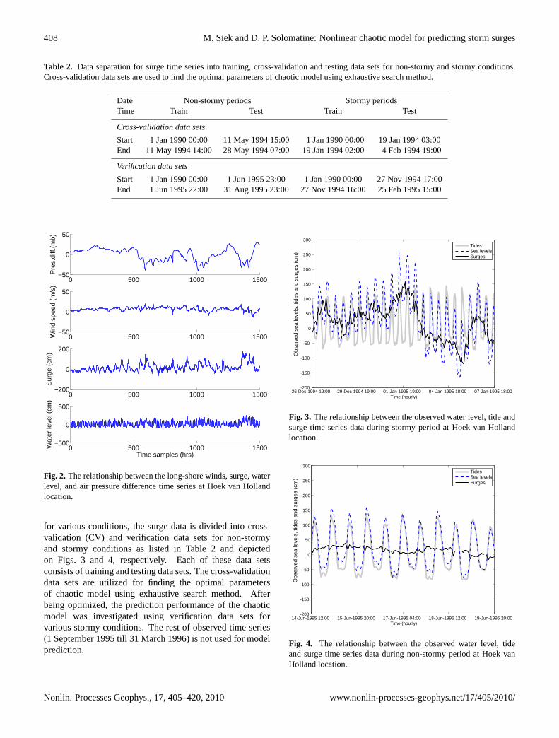
Fig. 4. The relationship between the observed water level, tide and surge time series data during non-stormy

period at Hoek van Holland location.

0 5 10 15 20 25 30 35 40 45 500

0.1

0.2

0.3

0.4

0.5

0.6

0.7

0.8

0.9

1

Time lags (hours)

Aut

ocor

rela

tion

and

mut

ual i

nfor

mat

ion

(in b

its/h

ours

)

AutocorrelationMutual information

Fig. 5. Autocorrelation function (dotted line with circles) and mutual information (solid line with triangles) as

a function of time lags suggesting the optimal time delay is 10 hours.

21

Fig. 4. The relationship between the observed water level, tideand surge time series data during non-stormy period at Hoek vanHolland location.



This data separation was made based on the analysisof recurrence plot and visual inspection in time-domaintime series. The recurrence plot is used to visualize therecurrences in a dynamical system, which it has capabilitiesto detect the presence of homogeneity, intermittency andtransition in a time series (Marwan et al., 2007).

3 Nonlinear dynamics and chaos theory

3.1 Dynamical system

A dynamical system can be defined as a set of rules ormathematical equations that describe the time evolution ofthe system states given some initial conditions or knowledgeof its previous history. Some examples of dynamical systemare the Navier-Stokes equations and Newton’s equations forthe motion of a particle with suitably specified forces. Thesedynamical systems can often be expressed bym-first orderordinary differential equationsdx/dt = f(x(t)) or in discretetime t = n1t by maps of the formxn+1 = f(xn). This timeevolution is defined in some phase space. Such nonlinearsystems can exhibit deterministic chaos which comprises aclass of a signal intermediate between regular sinusoidal orquasi-periodic motions and unpredictable or truly stochasticbehavior (Lorenz, 1963). The main reason for applyingchaos theory is the existence of methods permitting to predictthe future positions of the system in the state space.

3.2 Phase space reconstruction: method of time-delayembedding

The most important phase space reconstruction techniqueis the method of time delays, which is known as Takens’embedding theorem (Takens, 1981). Vectors in a new spaceor embedding space are formed by the time delayed valuesof the scalar measurements. According to Takens’ theorem,the dynamics of a time series can be fully embedded in them-dimensional phase space defined by the delayed vectors:

Yt ={xt ,xt−τ ,xt−2τ ,...,xt−(m−1)τ

}(2)

whereτ is the delay time. The lowest possible dimension ofsuch manifold is called an embedding dimension.

3.3 Finding appropriate time delay

In real applications, the delay timeτ needs to be appropri-ately chosen in order to fully capture the structure of theattractor. This can be achieved by embedding the attractorin a smooth manifold. The straightforward choice ofτ isusually made with the help of the zero-crossing autocorrela-tion function. However, in the terms of nonlinear methods,the choice ofτ associated with the first minimum of the timedelayed mutual information based on the Shanon’s entropy(Fraser and Swinney, 1986) demonstrates good performancein reconstructing the system dynamics from the observables.

14-Jun-1995 12:00 15-Jun-1995 20:00 17-Jun-1995 04:00 18-Jun-1995 12:00 19-Jun-1995 20:00-200

-150

-100

-50

0

50

100

150

200

250

300

Time (hourly)

Obs

erve

d se

a le

vels

, tid

es a

nd s

urge

s (c

m)


Fig. 4. The relationship between the observed water level, tide and surge time series data during non-stormy

period at Hoek van Holland location.

0 5 10 15 20 25 30 35 40 45 500

0.1

0.2

0.3

0.4

0.5

0.6

0.7

0.8

0.9

1

Time lags (hours)

Aut

ocor

rela

tion

and

mut

ual i

nfor

mat

ion

(in b

its/h

ours

)

AutocorrelationMutual information

Fig. 5. Autocorrelation function (dotted line with circles) and mutual information (solid line with triangles) as

a function of time lags suggesting the optimal time delay is 10 hours.

21

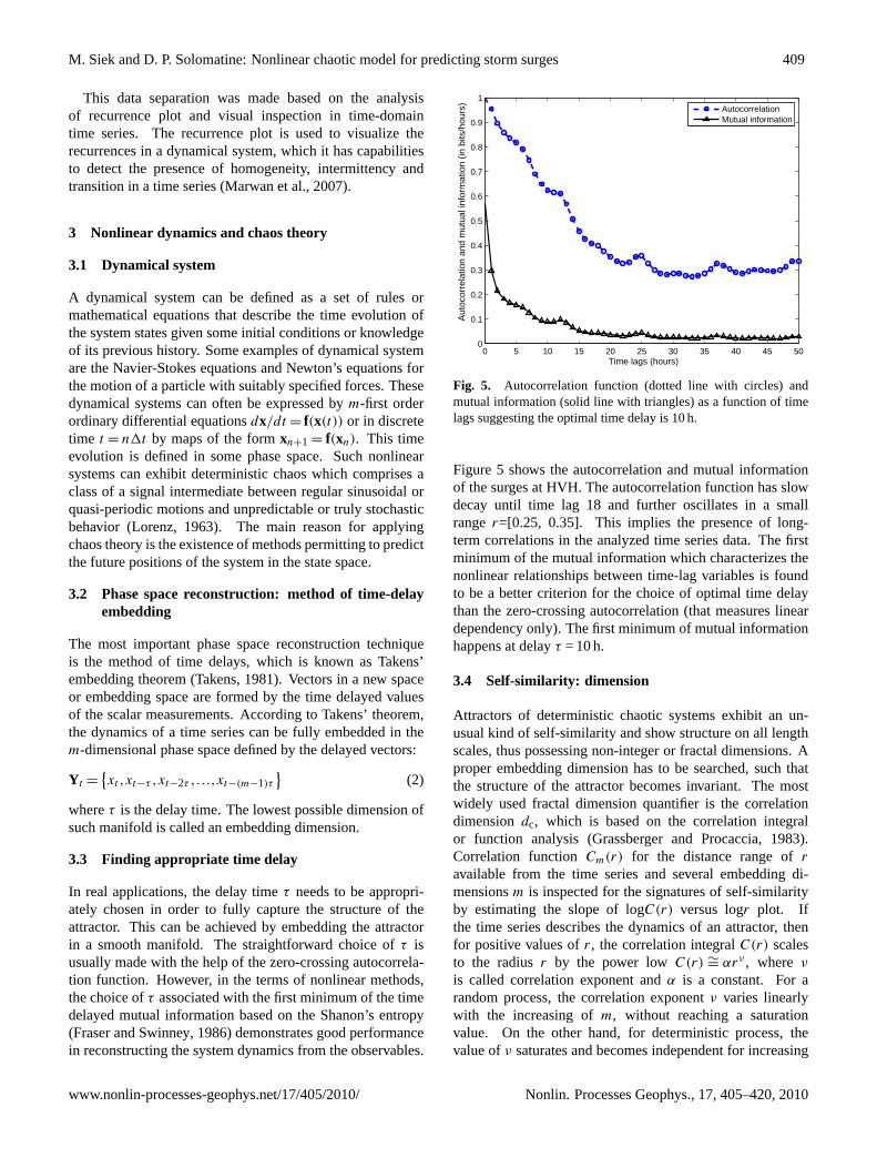
Fig. 5. Autocorrelation function (dotted line with circles) andmutual information (solid line with triangles) as a function of timelags suggesting the optimal time delay is 10 h.

Figure5 shows the autocorrelation and mutual informationof the surges at HVH. The autocorrelation function has slowdecay until time lag 18 and further oscillates in a smallranger=[0.25, 0.35]. This implies the presence of long-term correlations in the analyzed time series data. The firstminimum of the mutual information which characterizes thenonlinear relationships between time-lag variables is foundto be a better criterion for the choice of optimal time delaythan the zero-crossing autocorrelation (that measures lineardependency only). The first minimum of mutual informationhappens at delayτ = 10 h.

3.4 Self-similarity: dimension

Attractors of deterministic chaotic systems exhibit an un-usual kind of self-similarity and show structure on all lengthscales, thus possessing non-integer or fractal dimensions. Aproper embedding dimension has to be searched, such thatthe structure of the attractor becomes invariant. The mostwidely used fractal dimension quantifier is the correlationdimensiondc, which is based on the correlation integralor function analysis (Grassberger and Procaccia, 1983).Correlation functionCm(r) for the distance range ofravailable from the time series and several embedding di-mensionsm is inspected for the signatures of self-similarityby estimating the slope of logC(r) versus logr plot. Ifthe time series describes the dynamics of an attractor, thenfor positive values ofr, the correlation integralC(r) scalesto the radiusr by the power lowC(r) ∼= αrν , where ν

is called correlation exponent andα is a constant. For arandom process, the correlation exponentν varies linearlywith the increasing ofm, without reaching a saturationvalue. On the other hand, for deterministic process, thevalue ofν saturates and becomes independent for increasing



Fig. 6. Correlation integral (sum) with the increasing embedding dimensions for the hourly surge time series

at Hoek van Holland. The correlation integral was computed for different embedding dimensions (the line with

squares corresponds to embedding dimension 2 and the line with star corresponds to embedding dimension 20).

2 4 6 8 10 12 14 16 18 200

1

2

3

4

5

6

7

8

9

10

Embedding dimension (m)

Cor

rela

tion

expo

nent

(ν)

Fig. 7. Relationship between the correlation exponentν and embedding dimensionm. Correlation exponent

increases with an increase of the embedded dimension up to a certain value and further saturates. The saturation

value of the correlation exponent, that is the correlation dimension, is about 8.5.

22

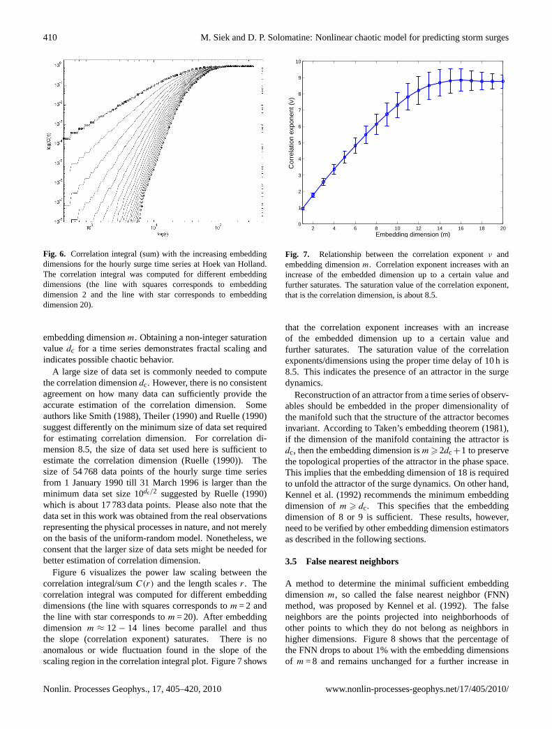
Fig. 6. Correlation integral (sum) with the increasing embeddingdimensions for the hourly surge time series at Hoek van Holland.The correlation integral was computed for different embeddingdimensions (the line with squares corresponds to embeddingdimension 2 and the line with star corresponds to embeddingdimension 20).

embedding dimensionm. Obtaining a non-integer saturationvalue dc for a time series demonstrates fractal scaling andindicates possible chaotic behavior.

A large size of data set is commonly needed to computethe correlation dimensiondc. However, there is no consistentagreement on how many data can sufficiently provide theaccurate estimation of the correlation dimension. Someauthors likeSmith(1988), Theiler(1990) andRuelle(1990)suggest differently on the minimum size of data set requiredfor estimating correlation dimension. For correlation di-mension 8.5, the size of data set used here is sufficient toestimate the correlation dimension (Ruelle (1990)). Thesize of 54 768 data points of the hourly surge time seriesfrom 1 January 1990 till 31 March 1996 is larger than theminimum data set size 10dc/2 suggested byRuelle (1990)which is about 17 783 data points. Please also note that thedata set in this work was obtained from the real observationsrepresenting the physical processes in nature, and not merelyon the basis of the uniform-random model. Nonetheless, weconsent that the larger size of data sets might be needed forbetter estimation of correlation dimension.

Figure 6 visualizes the power law scaling between thecorrelation integral/sumC(r) and the length scalesr. Thecorrelation integral was computed for different embeddingdimensions (the line with squares corresponds tom = 2 andthe line with star corresponds tom = 20). After embeddingdimension m ≈ 12− 14 lines become parallel and thusthe slope (correlation exponent) saturates. There is noanomalous or wide fluctuation found in the slope of thescaling region in the correlation integral plot. Figure7 shows

Fig. 6. Correlation integral (sum) with the increasing embedding dimensions for the hourly surge time series

at Hoek van Holland. The correlation integral was computed for different embedding dimensions (the line with

squares corresponds to embedding dimension 2 and the line with star corresponds to embedding dimension 20).

2 4 6 8 10 12 14 16 18 200

1

2

3

4

5

6

7

8

9

10


Cor

rela

tion

expo

nent

(ν)

Fig. 7. Relationship between the correlation exponentν and embedding dimensionm. Correlation exponent

increases with an increase of the embedded dimension up to a certain value and further saturates. The saturation

value of the correlation exponent, that is the correlation dimension, is about 8.5.

22

Fig. 7. Relationship between the correlation exponentν andembedding dimensionm. Correlation exponent increases with anincrease of the embedded dimension up to a certain value andfurther saturates. The saturation value of the correlation exponent,that is the correlation dimension, is about 8.5.

that the correlation exponent increases with an increaseof the embedded dimension up to a certain value andfurther saturates. The saturation value of the correlationexponents/dimensions using the proper time delay of 10 h is8.5. This indicates the presence of an attractor in the surgedynamics.

Reconstruction of an attractor from a time series of observ-ables should be embedded in the proper dimensionality ofthe manifold such that the structure of the attractor becomesinvariant. According to Taken’s embedding theorem (1981),if the dimension of the manifold containing the attractor isdc, then the embedding dimension ism > 2dc+1 to preservethe topological properties of the attractor in the phase space.This implies that the embedding dimension of 18 is requiredto unfold the attractor of the surge dynamics. On other hand,Kennel et al.(1992) recommends the minimum embeddingdimension ofm > dc. This specifies that the embeddingdimension of 8 or 9 is sufficient. These results, however,need to be verified by other embedding dimension estimatorsas described in the following sections.

3.5 False nearest neighbors

A method to determine the minimal sufficient embeddingdimensionm, so called the false nearest neighbor (FNN)method, was proposed byKennel et al.(1992). The falseneighbors are the points projected into neighborhoods ofother points to which they do not belong as neighbors inhigher dimensions. Figure8 shows that the percentage ofthe FNN drops to about 1% with the embedding dimensionsof m = 8 and remains unchanged for a further increase in



1 2 3 4 5 6 7 8 9 1010

-3

10-2

10-1

100


Fra

ctio

ns o

f fal

se n

eigh

bour

s

Fig. 8. The false nearest neighbors fractions as a function of embedding dimension.

0 5 10 15 20 25 300

0.2

0.4

0.6

0.8

1


E1(

m),

E*(

m)

E1(m)E*(m)

Fig. 9. Minimum embedding dimension estimated by Cao’s method withτ = 10 andk = 1.

23

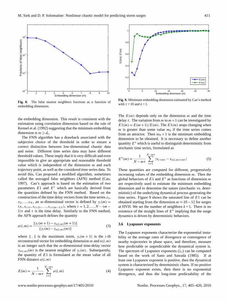
Fig. 8. The false nearest neighbors fractions as a function ofembedding dimension.

the embedding dimension. This result is consistent with theestimation using correlation dimension based on the rule ofKennel et al.(1992) suggesting that the minimum embeddingdimension ism > dc.

The FNN algorithm has a drawback associated with thesubjective choice of the threshold in order to ensure acorrect distinction between low-dimensional chaotic dataand noise. Different time series data may have differentthreshold values. These imply that it is very difficult and evenimpossible to give an appropriate and reasonable thresholdvalue which is independent of the dimensionm and eachtrajectory point, as well as the considered time series data. Toavoid this, Cao proposed a modified algorithm, sometimescalled the averaged false neighbors (AFN) method (Cao,1997). Cao’s approach is based on the estimation of twoparametersE1 and E∗ which are basically derived fromthe quantities defined by the FNN method. Based on theconstruction of the time delay vectors from the time seriesx1,x2,...,xN , an m-dimensional vector is defined byyi(m) =

(xi,xi+τ ,xi+2τ ,...,xi+(m−1)τ ), wherei = 1,2,...,N − (m−

1)τ andτ is the time delay. Similarly to the FNN method,the AFN approach defines the quantity

a(i,m)=‖yi(m+1)−yn(i,m)(m+1)‖

‖yi(m)−yn(i,m)(m)‖(3)

where ‖ . ‖ is the maximum norm,yi(m + 1) is the i-threconstructed vector for embedding dimensionm andn(i,m)

is an integer such that them-dimensional time-delay vectoryn(i,m)(m) is the nearest neighbor ofyi(m). Subsequently,the quantity ofE1 is formulated as the mean value of allFNN distancea(i,m)

E(m) =1

N −mτ

N−mτ∑i=1

a(i,m) (4)

1 2 3 4 5 6 7 8 9 1010

-3

10-2

10-1

100


Fra

ctio

ns o

f fal

se n

eigh

bour

s

Fig. 8. The false nearest neighbors fractions as a function of embedding dimension.

0 5 10 15 20 25 300

0.2

0.4

0.6

0.8

1


E1(

m),

E*(

m)

E1(m)E*(m)

Fig. 9. Minimum embedding dimension estimated by Cao’s method withτ = 10 andk = 1.

23

Fig. 9. Minimum embedding dimension estimated by Cao’s methodwith τ = 10 andk = 1.

The E(m) depends only on the dimensionm and the timedelayτ . The variation fromm tom+1 can be investigated byE1(m) = E(m+1)/E(m). TheE1(m) stops changing whenm is greater than some valuem0 if the time series comesfrom an attractor. Thenm0 +1 is the minimum embeddingdimension to be obtained. It is necessary to define anotherquantityE∗ which is useful to distinguish deterministic fromstochastic time series, formulated as

E∗(m) =1

N −mτ

N−mτ∑i=1

|xi+mτ −xn(i,m)+mτ | (5)

These quantities are computed for different, progressivelyincreasing values of the embedding dimensionm. Then theglobal behaviors ofE1 andE∗ as functions of dimensionmare respectively used to estimate the minimum embeddingdimension and to determine the nature (stochastic vs. deter-ministic) of the underlying dynamical process generating thetime series. Figure9 shows the saturated line ofE1 can beobtained starting from the dimensionm ≈ 10−12 for surgesat HVH. We set the number of neighborsk = 1. There is noexistence of the straight lines ofE∗ implying that the surgedynamics is driven by deterministic behaviors.

3.6 Lyapunov exponents

The Lyapunov exponents characterize the exponential insta-bility or the average rates of divergence or convergence ofnearby trajectories in phase space, and therefore, measurehow predictable or unpredictable the dynamical system is.The spectrum of Lyapunov exponents (λi) can be computedbased on the work ofSano and Sawada(1985). If atleast one Lyapunov exponent is positive, then the dynamicalsystem is characterized by deterministic chaos. If no positiveLyapunov exponent exists, then there is no exponentialdivergence, and thus the long-time predictability of the



0.5 1 1.5 2 2.5 3 3.5 4 4.5 5

x 104

-1.6

-1.4

-1.2

-1

-0.8

-0.6

-0.4

-0.2

0

0.2

Length (time samples)

Lyap

unov

exp

onen

ts (

in b

its/h

ours

)

Lyp1

Lyp2

Lyp3

Lyp4

Lyp5

Lyp6

Lyp7

Lyp8

Sum(Lyp)

Fig. 10. The largest Lyapunov exponent (lines with circles) is positive and the sum of global Lyapunov expo-

nents (lines with triangle) is negative.

24

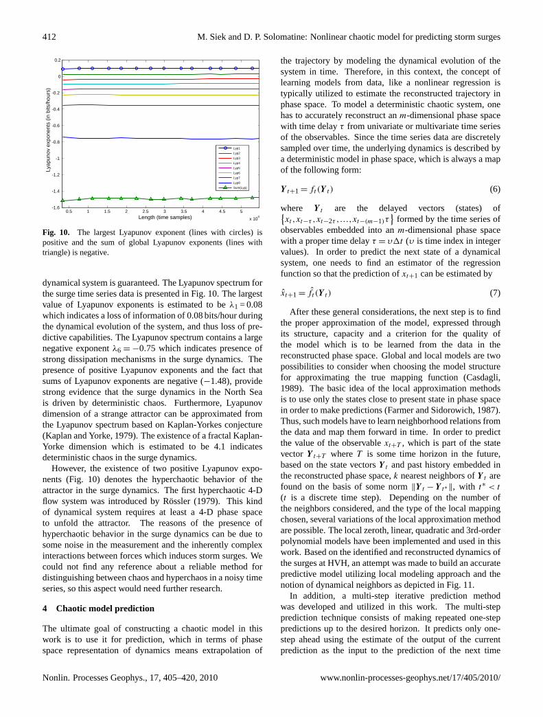
Fig. 10. The largest Lyapunov exponent (lines with circles) ispositive and the sum of global Lyapunov exponents (lines withtriangle) is negative.

dynamical system is guaranteed. The Lyapunov spectrum forthe surge time series data is presented in Fig.10. The largestvalue of Lyapunov exponents is estimated to beλ1 = 0.08which indicates a loss of information of 0.08 bits/hour duringthe dynamical evolution of the system, and thus loss of pre-dictive capabilities. The Lyapunov spectrum contains a largenegative exponentλ6 = −0.75 which indicates presence ofstrong dissipation mechanisms in the surge dynamics. Thepresence of positive Lyapunov exponents and the fact thatsums of Lyapunov exponents are negative (−1.48), providestrong evidence that the surge dynamics in the North Seais driven by deterministic chaos. Furthermore, Lyapunovdimension of a strange attractor can be approximated fromthe Lyapunov spectrum based on Kaplan-Yorkes conjecture(Kaplan and Yorke, 1979). The existence of a fractal Kaplan-Yorke dimension which is estimated to be 4.1 indicatesdeterministic chaos in the surge dynamics.

However, the existence of two positive Lyapunov expo-nents (Fig.10) denotes the hyperchaotic behavior of theattractor in the surge dynamics. The first hyperchaotic 4-Dflow system was introduced byRossler(1979). This kindof dynamical system requires at least a 4-D phase spaceto unfold the attractor. The reasons of the presence ofhyperchaotic behavior in the surge dynamics can be due tosome noise in the measurement and the inherently complexinteractions between forces which induces storm surges. Wecould not find any reference about a reliable method fordistinguishing between chaos and hyperchaos in a noisy timeseries, so this aspect would need further research.

4 Chaotic model prediction

The ultimate goal of constructing a chaotic model in thiswork is to use it for prediction, which in terms of phasespace representation of dynamics means extrapolation of

the trajectory by modeling the dynamical evolution of thesystem in time. Therefore, in this context, the concept oflearning models from data, like a nonlinear regression istypically utilized to estimate the reconstructed trajectory inphase space. To model a deterministic chaotic system, onehas to accurately reconstruct anm-dimensional phase spacewith time delayτ from univariate or multivariate time seriesof the observables. Since the time series data are discretelysampled over time, the underlying dynamics is described bya deterministic model in phase space, which is always a mapof the following form:

Y t+1 = ft (Y t ) (6)

where Y t are the delayed vectors (states) of{xt ,xt−τ ,xt−2τ ,...,xt−(m−1)τ

}formed by the time series of

observables embedded into anm-dimensional phase spacewith a proper time delayτ = υ1t (υ is time index in integervalues). In order to predict the next state of a dynamicalsystem, one needs to find an estimator of the regressionfunction so that the prediction ofxt+1 can be estimated by

xt+1 = ft (Y t ) (7)

After these general considerations, the next step is to findthe proper approximation of the model, expressed throughits structure, capacity and a criterion for the quality ofthe model which is to be learned from the data in thereconstructed phase space. Global and local models are twopossibilities to consider when choosing the model structurefor approximating the true mapping function (Casdagli,1989). The basic idea of the local approximation methodsis to use only the states close to present state in phase spacein order to make predictions (Farmer and Sidorowich, 1987).Thus, such models have to learn neighborhood relations fromthe data and map them forward in time. In order to predictthe value of the observablext+T , which is part of the statevector Y t+T whereT is some time horizon in the future,based on the state vectorsY t and past history embedded inthe reconstructed phase space,k nearest neighbors ofY t arefound on the basis of some norm‖Y t −Y t∗‖, with t∗ < t

(t is a discrete time step). Depending on the number ofthe neighbors considered, and the type of the local mappingchosen, several variations of the local approximation methodare possible. The local zeroth, linear, quadratic and 3rd-orderpolynomial models have been implemented and used in thiswork. Based on the identified and reconstructed dynamics ofthe surges at HVH, an attempt was made to build an accuratepredictive model utilizing local modeling approach and thenotion of dynamical neighbors as depicted in Fig.11.

In addition, a multi-step iterative prediction methodwas developed and utilized in this work. The multi-stepprediction technique consists of making repeated one-steppredictions up to the desired horizon. It predicts only one-step ahead using the estimate of the output of the currentprediction as the input to the prediction of the next time



0 5 10 15 20 25 30 35 40 45

-50

0

50

100

Sea

wat

er le

vel (

in c

m)

Samples in time (in hours)(a) Time-domain time series of sea levels at Hoek van Holland

-80 -60 -40 -20 0 20 40 60 80 100

-50

0

50

100

-50

0

50

100

WL(t- τ)

WL(t-2* τ)(b) Phase space reconstruction with τ=3 and m=3

WL(

t)

t t+T

Starting point

Dynamical neighbours

Starting point

Current point (t)

Current point (t)

Prediction (t+T)

t- τt-2 τ

Building local model

r

Prediction t+T?

Fig. 11. (a) Time-domain time series of the sea levels at Hoek van Holland. Future state or prediction (black

empty circle marking) can be estimated by the self-similarity of the current point (black markings) with pre-

vious time-lag data points as defined in the phase space reconstruction (τ = 3,m = 3). Current point has

self-similarity (behavior) to the previous points (triangle and box markings) as indicated by left-arrow dashed

lines. (b) Phase space reconstruction and the description of searching dynamical neighbors and their dynamical

evolution in the past allowing for predicting the future evolution of the dynamics using local modeling. In this

example, the real sea level data reconstructed in3-dimensional phase space withτ = 3 hours is utilized. Three

data points (star and diamond markings) in time-domain time series are represented as a single point in phase

space. Prediction is made by searching the dynamical neighbors (triangle and box markings) of the current

point (black circle marking) in phase space and extrapolating the future state by using a local predictive model

constructed based on dynamical neighbors.

25

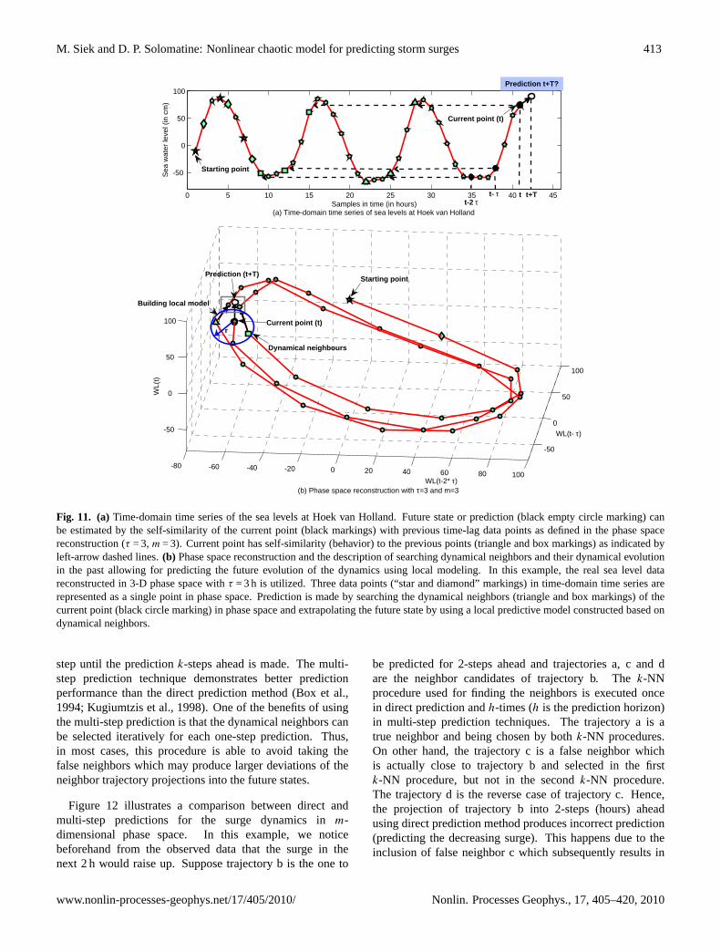
Fig. 11. (a)Time-domain time series of the sea levels at Hoek van Holland. Future state or prediction (black empty circle marking) canbe estimated by the self-similarity of the current point (black markings) with previous time-lag data points as defined in the phase spacereconstruction (τ = 3, m = 3). Current point has self-similarity (behavior) to the previous points (triangle and box markings) as indicated byleft-arrow dashed lines.(b) Phase space reconstruction and the description of searching dynamical neighbors and their dynamical evolutionin the past allowing for predicting the future evolution of the dynamics using local modeling. In this example, the real sea level datareconstructed in 3-D phase space withτ = 3 h is utilized. Three data points (“star and diamond” markings) in time-domain time series arerepresented as a single point in phase space. Prediction is made by searching the dynamical neighbors (triangle and box markings) of thecurrent point (black circle marking) in phase space and extrapolating the future state by using a local predictive model constructed based ondynamical neighbors.

step until the predictionk-steps ahead is made. The multi-step prediction technique demonstrates better predictionperformance than the direct prediction method (Box et al.,1994; Kugiumtzis et al., 1998). One of the benefits of usingthe multi-step prediction is that the dynamical neighbors canbe selected iteratively for each one-step prediction. Thus,in most cases, this procedure is able to avoid taking thefalse neighbors which may produce larger deviations of theneighbor trajectory projections into the future states.

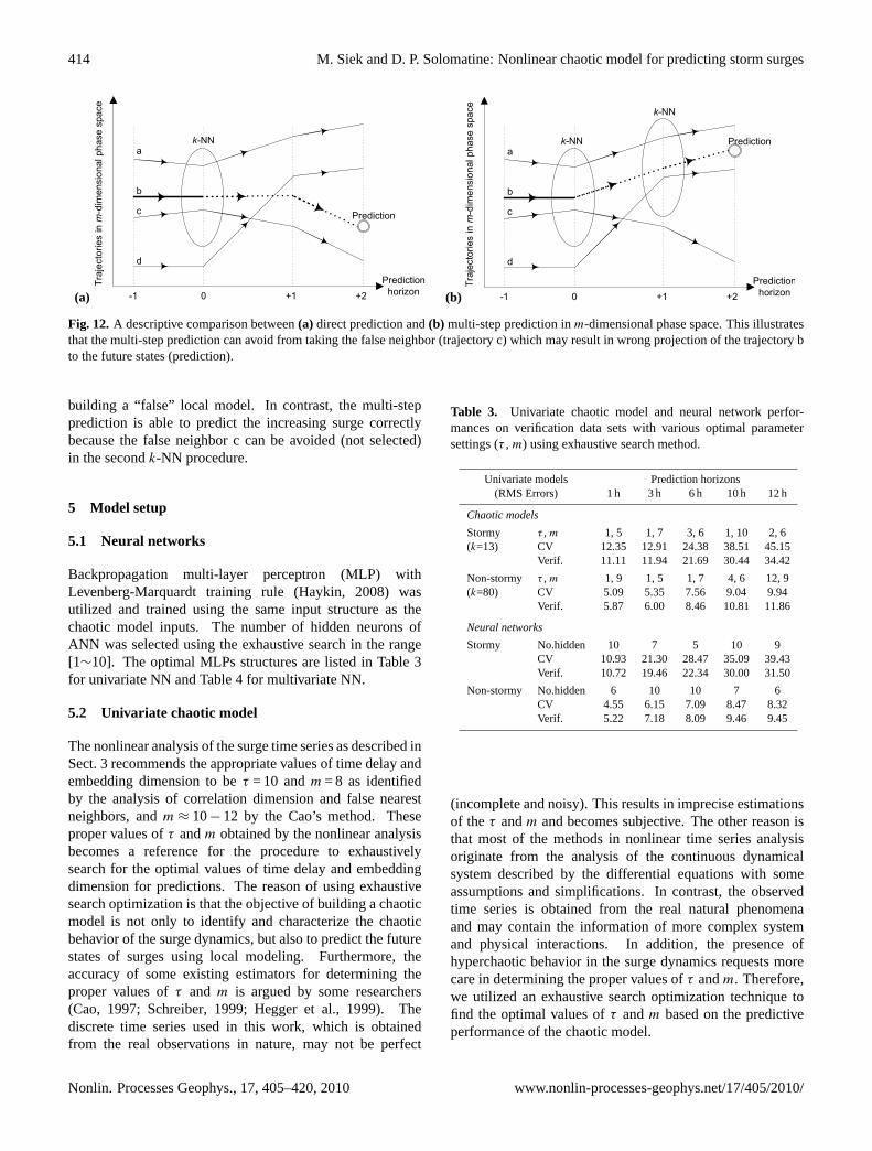
Figure 12 illustrates a comparison between direct andmulti-step predictions for the surge dynamics inm-dimensional phase space. In this example, we noticebeforehand from the observed data that the surge in thenext 2 h would raise up. Suppose trajectory b is the one to

be predicted for 2-steps ahead and trajectories a, c and dare the neighbor candidates of trajectory b. Thek-NNprocedure used for finding the neighbors is executed oncein direct prediction andh-times (h is the prediction horizon)in multi-step prediction techniques. The trajectory a is atrue neighbor and being chosen by bothk-NN procedures.On other hand, the trajectory c is a false neighbor whichis actually close to trajectory b and selected in the firstk-NN procedure, but not in the secondk-NN procedure.The trajectory d is the reverse case of trajectory c. Hence,the projection of trajectory b into 2-steps (hours) aheadusing direct prediction method produces incorrect prediction(predicting the decreasing surge). This happens due to theinclusion of false neighbor c which subsequently results in



(a)

Fig. 12.A descriptive comparison between (a) direct prediction and (b) multi-step prediction inm-dimensional

phase space. This illustrates that the multi-step prediction can avoid from taking the false neighbor (trajectory

c) which may result in wrong projection of the trajectoryb to the future states (prediction).

26

(b)

Fig. 12.A descriptive comparison between (a) direct prediction and (b) multi-step prediction inm-dimensional

phase space. This illustrates that the multi-step prediction can avoid from taking the false neighbor (trajectory

c) which may result in wrong projection of the trajectoryb to the future states (prediction).

26

Fig. 12. A descriptive comparison between(a) direct prediction and(b) multi-step prediction inm-dimensional phase space. This illustratesthat the multi-step prediction can avoid from taking the false neighbor (trajectory c) which may result in wrong projection of the trajectory bto the future states (prediction).

building a “false” local model. In contrast, the multi-stepprediction is able to predict the increasing surge correctlybecause the false neighbor c can be avoided (not selected)in the secondk-NN procedure.

5 Model setup

5.1 Neural networks

Backpropagation multi-layer perceptron (MLP) withLevenberg-Marquardt training rule (Haykin, 2008) wasutilized and trained using the same input structure as thechaotic model inputs. The number of hidden neurons ofANN was selected using the exhaustive search in the range[1∼10]. The optimal MLPs structures are listed in Table3for univariate NN and Table4 for multivariate NN.

5.2 Univariate chaotic model

The nonlinear analysis of the surge time series as described inSect. 3 recommends the appropriate values of time delay andembedding dimension to beτ = 10 andm = 8 as identifiedby the analysis of correlation dimension and false nearestneighbors, andm ≈ 10− 12 by the Cao’s method. Theseproper values ofτ andm obtained by the nonlinear analysisbecomes a reference for the procedure to exhaustivelysearch for the optimal values of time delay and embeddingdimension for predictions. The reason of using exhaustivesearch optimization is that the objective of building a chaoticmodel is not only to identify and characterize the chaoticbehavior of the surge dynamics, but also to predict the futurestates of surges using local modeling. Furthermore, theaccuracy of some existing estimators for determining theproper values ofτ and m is argued by some researchers(Cao, 1997; Schreiber, 1999; Hegger et al., 1999). Thediscrete time series used in this work, which is obtainedfrom the real observations in nature, may not be perfect

Table 3. Univariate chaotic model and neural network perfor-mances on verification data sets with various optimal parametersettings (τ , m) using exhaustive search method.

Univariate models Prediction horizons(RMS Errors) 1 h 3 h 6 h 10 h 12 h

Chaotic models

Stormy τ , m 1, 5 1, 7 3, 6 1, 10 2, 6(k=13) CV 12.35 12.91 24.38 38.51 45.15

Verif. 11.11 11.94 21.69 30.44 34.42

Non-stormy τ , m 1, 9 1, 5 1, 7 4, 6 12, 9(k=80) CV 5.09 5.35 7.56 9.04 9.94

Verif. 5.87 6.00 8.46 10.81 11.86

Neural networks

Stormy No.hidden 10 7 5 10 9CV 10.93 21.30 28.47 35.09 39.43Verif. 10.72 19.46 22.34 30.00 31.50

Non-stormy No.hidden 6 10 10 7 6CV 4.55 6.15 7.09 8.47 8.32Verif. 5.22 7.18 8.09 9.46 9.45

(incomplete and noisy). This results in imprecise estimationsof theτ andm and becomes subjective. The other reason isthat most of the methods in nonlinear time series analysisoriginate from the analysis of the continuous dynamicalsystem described by the differential equations with someassumptions and simplifications. In contrast, the observedtime series is obtained from the real natural phenomenaand may contain the information of more complex systemand physical interactions. In addition, the presence ofhyperchaotic behavior in the surge dynamics requests morecare in determining the proper values ofτ andm. Therefore,we utilized an exhaustive search optimization technique tofind the optimal values ofτ andm based on the predictiveperformance of the chaotic model.



Table 4. Multivariate chaotic model and neural network performances on verification data sets with various optimal parameter settings (τ ,m) using exhaustive search method.

Multivariate Phase Space Reconstruction Multivariate Chaotic Models Multivariate Neural Networks

PHoriz Surge WL Surge Wind Press RMSE RMSE No. RMSE RMSE

(hours) (hvh) (hvh) (epf) (hvh) (hvh)τ , m τ , m τ , m τ , m τ , m k (CV) (Verif.) Hid. (CV) (Verif.)

Stormy condition1 10, 8 4, 6 1, 5 5, 5 4, 5 13 15.52 8.81 5 6.48 6.533 10, 8 4, 6 3, 4 2, 2 1, 4 13 22.21 11.99 7 15.87 16.786 10, 8 4, 6 3, 5 4, 5 5, 2 13 37.96 21.12 8 22.24 20.4510 10, 8 4, 6 3, 5 5, 5 5, 3 13 43.45 31.32 8 28.05 30.3712 10, 8 4, 6 4, 4 3, 2 1, 2 13 47.28 34.80 8 28.74 28.09

Non-stormy condition1 10, 8 4, 6 1, 4 2, 4 1, 5 80 3.40 4.79 5 4.20 4.763 10, 8 4, 6 1, 2 2, 4 2, 5 80 2.94 6.59 6 7.75 8.696 10, 8 4, 6 1, 5 4, 2 5, 5 80 6.69 8.05 2 9.75 11.0210 10, 8 4, 6 1, 5 5, 2 1, 2 80 8.02 10.52 7 9.96 10.8412 10, 8 4, 6 1, 4 5, 2 5, 3 80 6.59 10.73 4 10.96 12.37

The other important parameter for building a chaoticmodel is the number of neighbors (k). Sensitivity analysiswas performed to find the properk values for non-stormyand stormy conditions. The sensitivity analysis was per-formed by setting up the chaotic model parameters for thesurges (with fixedτ = 10 andm = 8) andk run from 1 to2000. Subsequently, the exhaustive search optimization wasexecuted using the optimalk-value for finding the optimalvalues ofτ andm. The 3rd-order polynomial local modelswere built based on the dynamical neighbors. This modelshows better predictive performance for the local modelin comparison to the zeroth, linear and quadratic models.Additionally, we use also filtered out the neighbors that arefar (in Euclidean sense) from the current point – treatingthem as false neighbors. The procedure is as follows:

1. Define the number of neigbhours (k).

2. Find thek-nearest neigbhours of the current state in thephase space.

3. Remove the discovered neighbors if these neighborshave distance to the current state larger than twice thedistance for the 1-nearest neighbor.

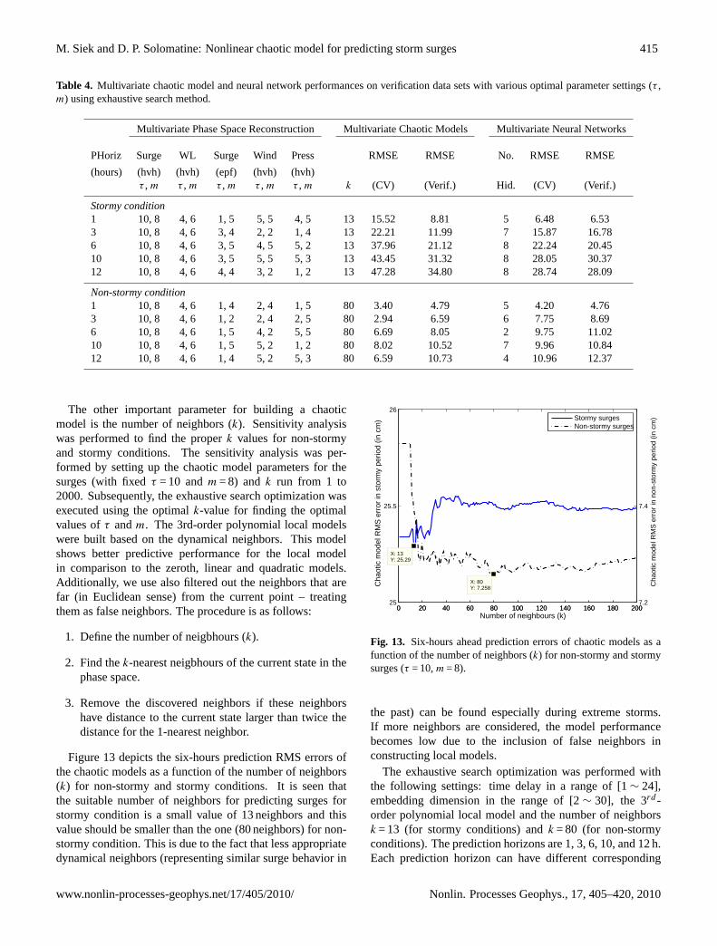
Figure13 depicts the six-hours prediction RMS errors ofthe chaotic models as a function of the number of neighbors(k) for non-stormy and stormy conditions. It is seen thatthe suitable number of neighbors for predicting surges forstormy condition is a small value of 13 neighbors and thisvalue should be smaller than the one (80 neighbors) for non-stormy condition. This is due to the fact that less appropriatedynamical neighbors (representing similar surge behavior in

0 20 40 60 80 100 120 140 160 180 20025

5.5

26

X: 13Y: 25.29

Number of neighbours (k)

Cha

otic

mod

el R

MS

err

or in

sto

rmy

perio

d (in

cm

)

2

0 20 40 60 80 100 120 140 160 180 2007.2

7.4

X: 80Y: 7.258

Cha

otic

mod

el R

MS

err

or in

non

-sto

rmy

perio

d (in

cm

)Stormy surgesNon-stormy surges

Fig. 13. Six-hours ahead prediction errors of chaotic models as a function of the number of neighbors (k) for

non-stormy and stormy surges (τ=10,m=8).

02

46

810

02

46

810

1212

14

16

18

20

22

Embedding dimension (m)Time delay (tau)

RM

SE

02

46

810

02

46

810

1238

40

42

44

46

48


RM

SE

Fig. 14.Univariate chaotic model: RMS errors for 1 hour (left) and 10 hours (right) prediction horizons during

stormy period as a function of time delay and embedding dimension.

27

Fig. 13. Six-hours ahead prediction errors of chaotic models as afunction of the number of neighbors (k) for non-stormy and stormysurges (τ = 10,m = 8).

the past) can be found especially during extreme storms.If more neighbors are considered, the model performancebecomes low due to the inclusion of false neighbors inconstructing local models.

The exhaustive search optimization was performed withthe following settings: time delay in a range of [1∼ 24],embedding dimension in the range of [2∼ 30], the 3rd -order polynomial local model and the number of neighborsk = 13 (for stormy conditions) andk = 80 (for non-stormyconditions). The prediction horizons are 1, 3, 6, 10, and 12 h.Each prediction horizon can have different corresponding



0 20 40 60 80 100 120 140 160 180 20025

25.5

26

X: 13Y: 25.29

Number of neighbours (k)

Cha

otic

mod

el R

MS

err

or in

sto

rmy

perio

d (in

cm

)

0 20 40 60 80 100 120 140 160 180 2007.2

7.4

X: 80Y: 7.258

Cha

otic

mod

el R

MS

err

or in

non

-sto

rmy

perio

d (in

cm

)

Stormy surgesNon-stormy surges

Fig. 13. Six-hours ahead prediction errors of chaotic models as a function of the number of neighbors (k) for

non-stormy and stormy surges (τ=10,m=8).

02

46

810

02

46

810

1212

14

16

18

20

22


RM

SE

02

46

810

02

46

810

1238

40

42

44

46

48


RM

SE

Fig. 14.Univariate chaotic model: RMS errors for 1 hour (left) and 10 hours (right) prediction horizons during

stormy period as a function of time delay and embedding dimension.

27

Fig. 14. Univariate chaotic model: RMS errors for 1 h (left) and 10 h (right) prediction horizons during stormy period as a function of timedelay and embedding dimension.

-50 -40 -30 -20 -10 0 10 20 30 40 500.2

0.3

0.4

0.5

0.6

0.7

0.8

0.9

1

Time lags (hrs)

Cor

rela

tion

coef

ficie

nt

EPFK13

-50 -40 -30 -20 -10 0 10 20 30 40 500

0.05

0.1

0.15

0.2

0.25

0.3

Time lags (hrs)

Mut

ual i

nfor

mat

ion

(bits

)

K13EPF

Fig. 15.Cross correlation (left) and mutual information (right) between surges at Hoek van Holland and neigh-

boring stations (EPF and K13). Both techniques show that the EPF surges precedes surges at HVH about

1 hour and the K13 surges has less relationship with HVH surges and the HVH surges would reach to K13

around 1–1.5 hours later.

-50 -40 -30 -20 -10 0 10 20 30 40 50-0.7

-0.6

-0.5

-0.4

-0.3

-0.2

-0.1

0

0.1

0.2

0.3

Time lags (hrs)

Cor

rela

tion

coef

ficie

nt

10

20

30

40

50

60

70

80

90

100

110

120

130

140

150

160

170

180

-50 -40 -30 -20 -10 0 10 20 30 40 500

0.02

0.04

0.06

0.08

0.1

0.12

Time lags (hrs)

Ave

rage

mut

ual i

nfor

mat

ion

(bits

)

102030405060708090100110120130140150160170180

Fig. 16. Cross correlation (left) and mutual information (right) between wind components and surge at Hoek

van Holland with various wind direction (0-180 degrees from North). The strongest influence of the winds on

the surge (correlation coefficient=-0.65) is generated by the120◦ wind component or the north-westerly wind.

Similarly, it is indicated by mutual information.

28

-50 -40 -30 -20 -10 0 10 20 30 40 500.2

0.3

0.4

0.5

0.6

0.7

0.8

0.9

1

Time lags (hrs)

Cor

rela

tion

coef

ficie

nt

EPFK13

-50 -40 -30 -20 -10 0 10 20 30 40 500

0.05

0.1

0.15

0.2

0.25

0.3

Time lags (hrs)

Mut

ual i

nfor

mat

ion

(bits

)

K13EPF





-50 -40 -30 -20 -10 0 10 20 30 40 50-0.7

-0.6

-0.5

-0.4

-0.3

-0.2

-0.1

0

0.1

0.2

0.3

Time lags (hrs)

Cor

rela

tion

coef

ficie

nt

10

20

30

40

50

60

70

80

90

100

110

120

130

140

150

160

170

180

-50 -40 -30 -20 -10 0 10 20 30 40 500

0.02

0.04

0.06

0.08

0.1

0.12

Time lags (hrs)

Ave

rage

mut

ual i

nfor

mat

ion

(bits

)

102030405060708090100110120130140150160170180





28

Fig. 15.Cross correlation (left) and mutual information (right) between surges at Hoek van Holland and neighboring stations (EPF and K13).Both techniques show that the EPF surges precedes surges at HVH about 1 hour and the K13 surges has less relationship with HVH surgesand the HVH surges would reach to K13 around 1–1.5 h later.

values of time delay and embedding dimension. Theoptimization result is the most accurate chaotic model whichhas the lowest RMS error on cross-validation data set. Thecross-validation data sets have a data set of 400 data points(see Table2): 19 January 1994 03:00 till 4 February 199419:00 (time indices of 35500–35900) for stormy conditionand 11 May 1994 15:00 till 28 May 1994 07:00 (timeindices of 38200–38600) for non-stormy condition. Thissmall size of cross-validation data sets was employed withconsiderations of the intensive computation required for theexhaustive search optimization.

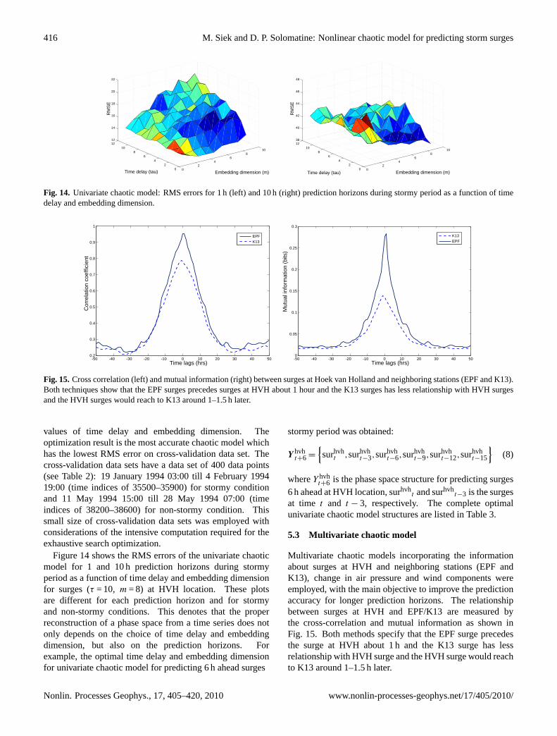
Figure14 shows the RMS errors of the univariate chaoticmodel for 1 and 10 h prediction horizons during stormyperiod as a function of time delay and embedding dimensionfor surges (τ = 10, m = 8) at HVH location. These plotsare different for each prediction horizon and for stormyand non-stormy conditions. This denotes that the properreconstruction of a phase space from a time series does notonly depends on the choice of time delay and embeddingdimension, but also on the prediction horizons. Forexample, the optimal time delay and embedding dimensionfor univariate chaotic model for predicting 6 h ahead surges

stormy period was obtained:

Y hvht+6 =

{surhvh

t ,surhvht−3,surhvh

t−6,surhvht−9,surhvh

t−12,surhvht−15

}(8)

whereY hvht+6 is the phase space structure for predicting surges

6 h ahead at HVH location, surhvht and surhvh

t−3 is the surgesat time t and t − 3, respectively. The complete optimalunivariate chaotic model structures are listed in Table3.

5.3 Multivariate chaotic model

Multivariate chaotic models incorporating the informationabout surges at HVH and neighboring stations (EPF andK13), change in air pressure and wind components wereemployed, with the main objective to improve the predictionaccuracy for longer prediction horizons. The relationshipbetween surges at HVH and EPF/K13 are measured bythe cross-correlation and mutual information as shown inFig. 15. Both methods specify that the EPF surge precedesthe surge at HVH about 1 h and the K13 surge has lessrelationship with HVH surge and the HVH surge would reachto K13 around 1–1.5 h later.



-50 -40 -30 -20 -10 0 10 20 30 40 500.2

0.3

0.4

0.5

0.6

0.7

0.8

0.9

1

Time lags (hrs)

Cor

rela

tion

coef

ficie

nt

EPFK13

-50 -40 -30 -20 -10 0 10 20 30 40 500

0.05

0.1

0.15

0.2

0.25

0.3

Time lags (hrs)

Mut

ual i

nfor

mat

ion

(bits

)

K13EPF





-50 -40 -30 -20 -10 0 10 20 30 40 50-0.7

-0.6

-0.5

-0.4

-0.3

-0.2

-0.1

0

0.1

0.2

0.3

Time lags (hrs)

Cor

rela

tion

coef

ficie

nt

10

20

30

40

50

60

70

80

90

100

110

120

130

140

150

160

170

180

-50 -40 -30 -20 -10 0 10 20 30 40 500

0.02

0.04

0.06

0.08

0.1

0.12

Time lags (hrs)

Ave

rage

mut

ual i

nfor

mat

ion

(bits

)

102030405060708090100110120130140150160170180





28

-50 -40 -30 -20 -10 0 10 20 30 40 500.2

0.3

0.4

0.5

0.6

0.7

0.8

0.9

1

Time lags (hrs)

Cor

rela

tion

coef

ficie

nt

EPFK13

-50 -40 -30 -20 -10 0 10 20 30 40 500

0.05

0.1

0.15

0.2

0.25

0.3

Time lags (hrs)

Mut

ual i

nfor

mat

ion

(bits

)

K13EPF





-50 -40 -30 -20 -10 0 10 20 30 40 50-0.7

-0.6

-0.5

-0.4

-0.3

-0.2

-0.1

0

0.1

0.2

0.3

Time lags (hrs)

Cor

rela

tion

coef

ficie

nt

10

20

30

40

50

60

70

80

90

100

110

120

130

140

150

160

170

180

-50 -40 -30 -20 -10 0 10 20 30 40 500

0.02

0.04

0.06

0.08

0.1

0.12

Time lags (hrs)

Ave

rage

mut

ual i

nfor

mat

ion

(bits

)

102030405060708090100110120130140150160170180





28

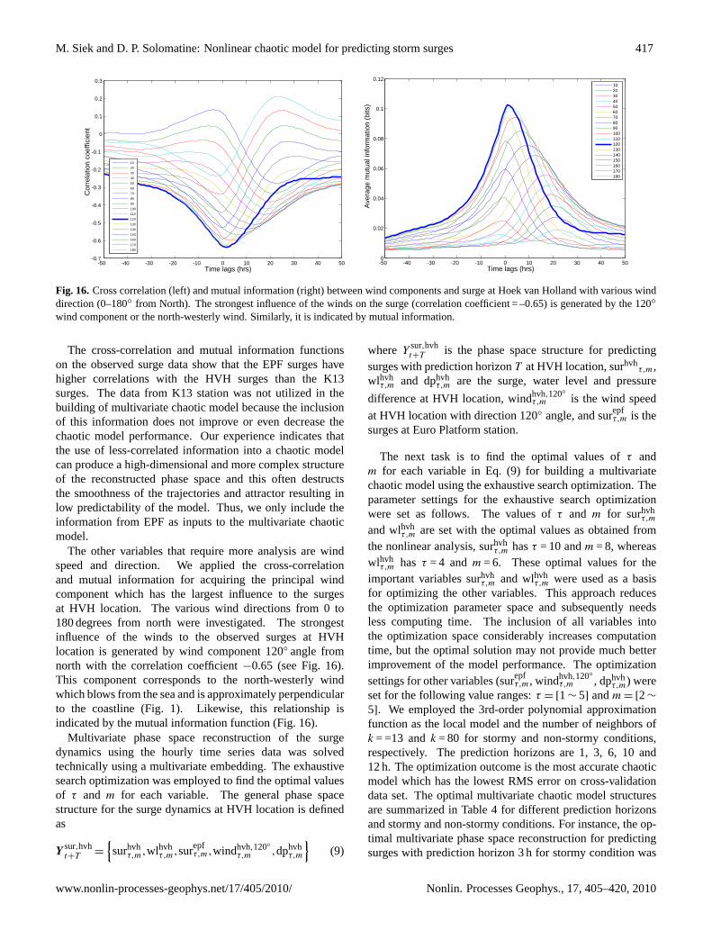
Fig. 16. Cross correlation (left) and mutual information (right) between wind components and surge at Hoek van Holland with various winddirection (0–180◦ from North). The strongest influence of the winds on the surge (correlation coefficient = –0.65) is generated by the 120◦

wind component or the north-westerly wind. Similarly, it is indicated by mutual information.

The cross-correlation and mutual information functionson the observed surge data show that the EPF surges havehigher correlations with the HVH surges than the K13surges. The data from K13 station was not utilized in thebuilding of multivariate chaotic model because the inclusionof this information does not improve or even decrease thechaotic model performance. Our experience indicates thatthe use of less-correlated information into a chaotic modelcan produce a high-dimensional and more complex structureof the reconstructed phase space and this often destructsthe smoothness of the trajectories and attractor resulting inlow predictability of the model. Thus, we only include theinformation from EPF as inputs to the multivariate chaoticmodel.

The other variables that require more analysis are windspeed and direction. We applied the cross-correlationand mutual information for acquiring the principal windcomponent which has the largest influence to the surgesat HVH location. The various wind directions from 0 to180 degrees from north were investigated. The strongestinfluence of the winds to the observed surges at HVHlocation is generated by wind component 120◦ angle fromnorth with the correlation coefficient−0.65 (see Fig.16).This component corresponds to the north-westerly windwhich blows from the sea and is approximately perpendicularto the coastline (Fig.1). Likewise, this relationship isindicated by the mutual information function (Fig.16).

Multivariate phase space reconstruction of the surgedynamics using the hourly time series data was solvedtechnically using a multivariate embedding. The exhaustivesearch optimization was employed to find the optimal valuesof τ and m for each variable. The general phase spacestructure for the surge dynamics at HVH location is definedas

Ysur,hvht+T =

{surhvh

τ,m,wlhvhτ,m,surepf

τ,m,windhvh,120◦τ,m ,dphvh

τ,m

}(9)

where Ysur,hvht+T is the phase space structure for predicting

surges with prediction horizonT at HVH location, surhvhτ,m,

wlhvhτ,m and dphvh

τ,m are the surge, water level and pressure

difference at HVH location, windhvh,120◦τ,m is the wind speed

at HVH location with direction 120◦ angle, and surepfτ,m is the

surges at Euro Platform station.

The next task is to find the optimal values ofτ andm for each variable in Eq. (9) for building a multivariatechaotic model using the exhaustive search optimization. Theparameter settings for the exhaustive search optimizationwere set as follows. The values ofτ and m for surhvh

τ,m

and wlhvhτ,m are set with the optimal values as obtained from

the nonlinear analysis, surhvhτ,m hasτ = 10 andm = 8, whereas

wlhvhτ,m has τ = 4 andm = 6. These optimal values for the

important variables surhvhτ,m and wlhvh

τ,m were used as a basisfor optimizing the other variables. This approach reducesthe optimization parameter space and subsequently needsless computing time. The inclusion of all variables intothe optimization space considerably increases computationtime, but the optimal solution may not provide much betterimprovement of the model performance. The optimizationsettings for other variables (surepf

τ,m, windhvh,120◦τ,m , dphvh

τ,m) wereset for the following value ranges:τ = [1∼ 5] andm = [2∼

5]. We employed the 3rd-order polynomial approximationfunction as the local model and the number of neighbors ofk = =13 andk = 80 for stormy and non-stormy conditions,respectively. The prediction horizons are 1, 3, 6, 10 and12 h. The optimization outcome is the most accurate chaoticmodel which has the lowest RMS error on cross-validationdata set. The optimal multivariate chaotic model structuresare summarized in Table4 for different prediction horizonsand stormy and non-stormy conditions. For instance, the op-timal multivariate phase space reconstruction for predictingsurges with prediction horizon 3 h for stormy condition was



200 400 600 800 1000 1200 1400 1600 1800 2000

-100

-50

0

50

100

150

Time samples (hourly)

Sur

ges

(cm

)

ActualUnivariate chaotic modelUnivariate neural networkMultivariate chaotic modelMultivariate neural network

200 400 600 800 1000 1200 1400 1600 1800 2000

-100

0

100

Time samples (1 hrs)

Uni

.CM

Err

or (

cm)

200 400 600 800 1000 1200 1400 1600 1800 2000

-100

0

100


Uni

.NN

Err

or (

cm)

200 400 600 800 1000 1200 1400 1600 1800 2000

-100

0

100


CM

Err

or (

cm)

200 400 600 800 1000 1200 1400 1600 1800 2000

-100

0

100


Mul

t.NN

Err

or (

cm)

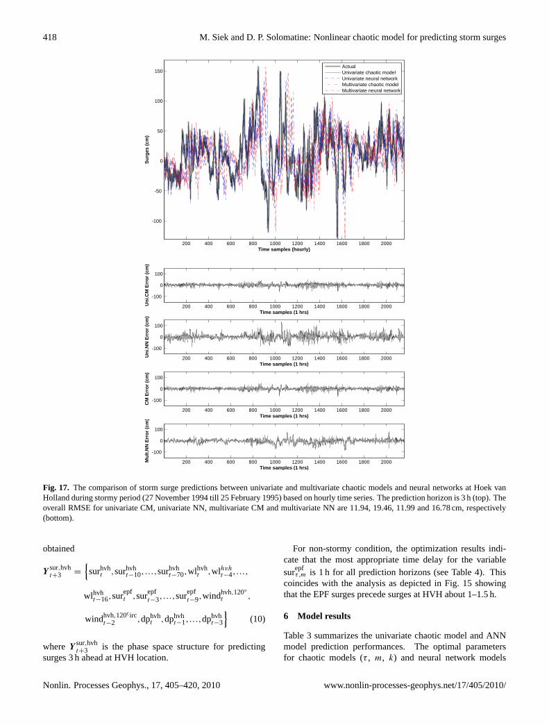
Fig. 17. The comparison of storm surge predictions between univariate and multivariate chaotic models and

neural networks at Hoek van Holland during stormy period (27-Nov-1994 till 25-Feb-1995) based on hourly

time series. The prediction horizon is 3 hours (top). The overall RMSE for univariate CM, univariate NN,

multivariate CM and multivariate NN are 11.94, 19.46, 11.99 and 16.78cm, respectively (bottom).

29

Fig. 17. The comparison of storm surge predictions between univariate and multivariate chaotic models and neural networks at Hoek vanHolland during stormy period (27 November 1994 till 25 February 1995) based on hourly time series. The prediction horizon is 3 h (top). Theoverall RMSE for univariate CM, univariate NN, multivariate CM and multivariate NN are 11.94, 19.46, 11.99 and 16.78 cm, respectively(bottom).

obtained

Ysur,hvht+3 =

{surhvh

t ,surhvht−10,...,surhvh

t−70,wlhvht ,wlhvh

t−4,...,

wlhvht−16,surepf

t ,surepft−3,...,surepf

t−9,windhvh,120◦t ,

windhvh,120circt−2 ,dphvh

t ,dphvht−1,...,dphvh

t−3

}(10)

where Ysur,hvht+3 is the phase space structure for predicting

surges 3 h ahead at HVH location.

For non-stormy condition, the optimization results indi-cate that the most appropriate time delay for the variablesurepf

τ,m is 1 h for all prediction horizons (see Table4). Thiscoincides with the analysis as depicted in Fig.15 showingthat the EPF surges precede surges at HVH about 1–1.5 h.

6 Model results

Table3 summarizes the univariate chaotic model and ANNmodel prediction performances. The optimal parametersfor chaotic models (τ , m, k) and neural network models



(number of hidden neurons) were obtained based on themodel performance (RMS error) on cross-validation data setsfor non-stormy and stormy conditions. Subsequently, weverified these models on verification data set with variousoptimal values ofτ , m, k and number of hidden neuronsbased on the prediction horizons and stormy and non-stormyconditions. These comparison results (up to 12 h prediction)show that both models have similar prediction accuracy, forboth stormy and non-stormy surge conditions. However, thechaotic model is able to predict the extreme surges better thanANN. This is depicted in Fig.17. The chaotic model errorsare more dampened and stable (also during the surge peaks)than the neural network errors.

Nonetheless, the predictive chaotic model with local mod-eling may include some false neighbors due to the fact thatthe trajectories are very close to each other and the nearestneighbors found may have different or reverse directionsof the trajectories. This is a practical problem occurringdue to the use of nonlinear discrete time series from theobservables and the use of integer (not fractal) values ofτ and m in phase space reconstruction. In the continuousdynamical system derived by the differential equations manyless false neighbors are to be found. The possible solutionsfor these issues are: to use smaller sampling time of thesurge data (e.g. 10 min) for reducing the sharp oscillationsand thus providing enough points for producing better localmodels to handle these oscillations; to implement a mixtureof various local models (e.g. ANN) in the phase space whichmay perform better for predicting future trajectories of aparticular condition or regime; to reconstruct the phase spacefrom a time series using non-equidistance time delay methodwhich can unfold the attractor better; and to select a largersize of cross-validation data set.

A multivariate chaotic model (Table4) with inclusion ofvarious variables (wind, air pressure and neighboring stationinformation) does not significantly improve the accuracy ofpredictions in comparison to a univariate chaotic model.This is in a way surprising and disappointing. We seethe reason for that in the fact that adding more variables(observed non-smooth data) to the phase space distortsthe smoothness of trajectories and attractor of the surgedynamics. This distortion may produce more false nearestneighbors resulting in less accurate predictions by localmodels.

For the location at Hoek van Holland, the overall 3 hahead surge prediction errors (RMSE) on verification datasets during stormy period for univariate CM, univariate NN,multvariate CM and multivariate NN are 11.94, 19.46, 11.99and 16.78 cm, respectively. In this respect, the multivariatechaotic model generally outperforms ANN models becauseit uses the other variables, spatial information and localmodels for predicting the future surges by identifying thepast behavior of the surge dynamics.

7 Conclusions

Based on the nonlinear chaos analysis, the surge dynamicsalong the Dutch coast can be characterized as deterministicchaos. The presence of the chaotic dynamics togetherwith the positive Lyapunov exponents implies that there arelimits of predictability for any model. However, short-termreliable predictions are possible. The chaotic behavior occursbecause the sea levels and surges are the result of a complex,coupled nonlinear dynamical system. If compared to ourearlier work (Solomatine et al., 2000; Velickov, 2004; Sieket al., 2008, see Sect. 1) in the present paper we employedextended data analysis methods and improved algorithms forpredictive models. A chaotic model with local modelingand multi-step prediction technique demonstrates a goodpredictive performance and can serve as an effective toolfor accurate and reliable short-term storm surge predictions.Further improvements in accuracy are expected if moresophisticated methods to identify the adequate nearest neigh-bors are used, and if a data assimilation scheme is added tothe presented method.

Acknowledgements.The work described in this manuscript waspartly supported by the Delft Cluster Research Programme of theDutch Government and UNESCO-IHE (project “Safety againstFlooding”). Authors would like also to thank M. Verlaan for veryuseful discussion.

Edited by: O. TalagrandReviewed by: R. V. Donner and another anonymous referee

References

Alexandersson, H., Schmith, T., Iden, K., and Tuomenvirta, H.:Long-term variations of the storm climate over NW Europe,Global Atmos. Ocean System, 6, 97–120, 1998.

Battjes, J. A. and Gerritsen, H.: Coastal modelling for flooddefence, Philos. Transact. A Math. Phys. Eng. Sci., 360(1796),1461–1475, 2002.

Bode, L. and Hardy, T. A.: Progress and recent developments instorm surge modeling, J. Hydraul. Eng.-ASCE, 123(4), 315–331,1997.

Box, G., Jenkins, G., and Reinsel, G.: Time series analysis:forecasting and control, Prentice Hall, NJ, USA, 1994.

Butler, A., Heffernan, J. E., Tawn, J. A., Flather, R. A., andHorsburgh, K. J.: Extreme value analysis of decadal variations instorm surge elevations, J. Marine Syst., 67(1-2), 189-200, 2007.

Cao, L.: Practical method for determining the minimum embeddingdimension of a scalar time series, Physica D, 110(1–2), 43–50,1997.

Casdagli, M.: Nonlinear prediction of chaotic time series, PhysicaD, 35(3), 335–356, 1989.

Donner, R. V. and Barbosa, S. M.: Nonlinear time series analysis inthe geosciences, in: Lecture Notes in Earth Sciences, vol. 112,Berlin Springer Verlag, 2008.

Dronkers, J. J.: Tidal computations in rivers and coastal waters,North Holland Publishing Company, Amsterdam, 1964.



Farmer, J. D. and Sidorowich, J. J.: Predicting chaotic time series,Phys. Rev. Lett., 59(8), 845–848, 1987.

Fermi E., Pasta J., and Ulam S.: Studies of nonlinear problems,I. Los Alamos Report, LA-1940, 1955.

Fraser, A. M. and Swinney, H. L.: Independent coordinates forstrange attractors from mutual information, Phys. Rev. A, 33(2),1134–1140, 1986.

Frison, T. W., Abarbanel, H. D. I., Earle, M. D., Schultz,J. R., and Scherer, W. D.: Chaos and predictability inocean water levels, J. Geophys. Res., 104(C4), 7935-7951,doi:10.1029/1998JC900104, 1999.

Gonnert, G., Dube, S. K., Murty, T., and Siefert, W.: Global stormsurges: theory, observations and applications, Die Kuste, 63, 1–623, 2001.

Grassberger, P. and Procaccia, I.: Measuring the strangeness ofstrange attractors, Physica D, 9(1–2), 189–208, 1983.

Haykin, S.: Neural networks: a comprehensive foundation, PrenticeHall, 2008.

Hegger, R., Kantz, H., and Schreiber, T.: Practical implementationof nonlinear time series methods: The TISEAN package, Chaos:An Interdisciplinary Journal of Nonlinear Science, 9(2), 413–435, 1999.

Kaplan, J. L. and Yorke, J. A.: Chaotic behavior of multidimen-sional difference equations, Lect. Notes Math., 730, 204–227,1979.

Kennel, M. B., Brown, R., and Abarbanel, H. D. I.: Deter-mining embedding dimension for phase-space reconstructionusing a geometrical construction, Phys. Rev. A, 45(6), 3403,doi:10.1103/PhysRevA.45.3403, 1992.

Korteweg D. J. and de Vries G.: On the change of form of longwaves advancing in a rectangular canal and on a new type oflong stationary waves, Philosophical Magazine 5th Series, 36,422–443, 1895.

Kugiumtzis, D., Lingjaerde, O. C., and Christophersen, N.:Regularized local linear prediction of chaotic time series, PhysicaD, 112(3–4), 344–360, 1998.

Li, Y. C.: Chaos in partial differential equations, International Press,Somerville, MA, USA, 2004.

Lorenz, E. N.: Deterministic nonperiodic flow, J. Atmos. Sci.,20(2), 130–141, 1963.

Marwan, N., Romano, M., Thiel, M., and Kurths, J.: Recurrenceplots for the analysis of complex systems, Phys. Rep., 438(5–6),237–329, 2007.

Prandle, D., Wolf, J., and Jacques, C. J. N.: Surge-tide interaction inthe Southern North Sea, Elsevier Oceanography Series, Elsevier,23, 161–185, 1978.

Rossler, O. E.: An equation for hyperchaos, Phys. Lett., 71A(2,3),155–157, 1979.

Ruelle, D.: Deterministic chaos: the science and the fiction, P. Roy.Soc. Lond. A, 427, 241–248, 1990.

Sano, M. and Sawada, Y.: Measurement of the Lyapunov spectrumfrom a chaotic time series, Phys. Rev. Lett., 55(10), 1082–1085,1985.

Schreiber, T.: Interdisciplinary application of nonlinear time seriesmethods, Phys. Rep., 308, 1–64, 1999.

Siek, M., Solomatine, D. P., and Velickov, S.: Multivariate chaoticmodels vs neural networks in predicting storm surge dynamics,Int. Joint Conferences on Neural Networks, Hong Kong, 2112–2119, 2008.

Simonnet, E., Dijkstra, H. A., and Ghil, M.: Bifurcation analysisof ocean, atmosphere and climate models, in: Handbook ofNumerical Analysis, 14, Special Volume on ComputationalMethods for the Ocean and the Atmosphere, 187–230, 2009.

Smith, L.: Intrinsic limits on dimension calculations, Phys. Lett. A,133, 283–288, 1988.

Solomatine, D. P., Rojas, C., Velickov, S., and Wust, H.: Chaostheory in predicting surge water levels in the North Sea, 4thInternational Conference on Hydroinformatics, Iowa, USA,2000.

Takens, F.: Detecting strange attractors in turbulence, DynamicalSystems and Turbulence, Warwick 1980, Lecture Notes inMathematics, 898, Springer, Berlin, 366–381, 1981.

Theiler, J.: Estimating fractal dimension, J. Opt. Soc. Am. A, 7(6),1055–1073, 1990.

Tsonis, A. A.: Chaos: from theory to applications, Plenum Press,New York, 1992.

Velickov, S.: Nonlinear dynamics and chaos with applications tohydrodynamics and hydrological modelling, Taylor & FrancisGroup, 2004.

Verlaan, M., Zijderveld, A., de Vries, H., and Kroos, J.: Operationalstorm surge forecasting in the Netherlands: developments in thelast decade, Philos. T. Roy. Soc. A, 363(1831), 1441–1453, 2005.

Walton, T. L.: Short term storm surge forecasting, J. Coastal Res.,21(3), 421–429, 2005.

Woodworth, P. L., Flather, R. A., Williams, J. A., Wakelin, S. L.,and Jevrejeva, S.: The dependence of UK extreme sea levels andstorm surges on the North Atlantic Oscillation, Cont. Shelf Res.,27(7), 935–946, 2007.

Zabusky, N. J. and Kruskal, M. D.: Interaction of solitons in acollisionless plasma and the recurrence of initial states, Phys.Rev. Lett., 15, 240–243, 1965.


Nonlinear chaotic model for predicting storm surges · Nonlinear chaotic model for predicting storm...

Documents

Transcript of Nonlinear chaotic model for predicting storm surges · Nonlinear chaotic model for predicting storm...