i

New Jersey Greenhouse Gas Inventory and

Reference Case Projections 1990-2020

November 2008

New Jersey Department of Environmental Protection Lisa P. Jackson, Commissioner Jon S. Corzine, Governor

i

Executive Summary This report was prepared in response to directives of Governor Corzine’s Executive Order 54 and the New Jersey Global Warming Response Act. This report presents a preliminary inventory and forecast of the State’s greenhouse gas (GHG) emissions from 1990 to 2020. The inventory and forecast estimates serve as a starting point to assist the State with an initial comprehensive understanding of New Jersey’s current and possible future GHG emissions, and thereby inform the identification and analysis of policy options for mitigating GHG emissions. The Global Warming Response Act directs DEP to evaluate and recommend such policy options.

A draft of this report was posted on the New Jersey Global Warming website (http://www.state.nj.us/globalwarming/index.shtml) in February, 2008. Numerous comments and recommendations were received. The DEP has reviewed these comments and has made several improvements to the inventory and forecasts as a result. A summary of the most significant comments and the DEP’s responses are presented in Appendix I of this report. The BPU, in its Energy Master Plan (http://www.nj.gov/emp), has provided updates to the energy use data and projections that were used to estimate some of the GHG emissions in the February, 2008 draft report. These most recent data and projections have been used in preparing this report. Emissions and Reference Case Projections (Business-as-Usual) New Jersey’s anthropogenic GHG emissions and anthropogenic sinks (carbon storage) were estimated for the period from 1990 to 2020. Historical GHG emission estimates (1990 through 2005) were developed using a set of generally accepted principles and guidelines for state GHG emissions estimates (both historical and forecasted), with adjustments as needed to provide New Jersey-specific data and inputs when it was possible to do so. The initial reference case projections (2006-2020) are based on a compilation of various existing projections of electricity generation, fuel use, and other GHG-emitting activities, along with a set of transparent assumptions.

Activities in New Jersey accounted for approximately 142.1 million metric tons (MMt) of gross1 carbon dioxide equivalent (CO2eq) emissions (consumption basis) in 2005, an amount equal to about 2.0% of total US gross GHG emissions (based on 2005 US data).2 New Jersey’s gross GHG emissions are rising at a slower rate than those of the nation as a whole (gross emissions exclude carbon sinks, such as forests). New Jersey’s gross GHG emissions increased by about 9% from 1990 to 2005, while national emissions rose by 16% from 1990 to 2005. The growth in New Jersey’s emissions from 1990 to 2005 is primarily associated with the transportation and electricity consumption sectors.

Estimates of carbon sinks within New Jersey’s forests have also been included in this report. For forests, the current estimates indicate that about 6.7 MMTCO2eq was stored in New Jersey forest biomass in 2005. This leads to net emissions of 135.3 MMTCO2eq in New Jersey in 2005.

1 Excluding GHG emissions removed due to forestry and other land uses. 2 The national emissions used for these comparisons are based on 2005 emissions; (http://www.epa.gov/climatechange/emissions/usinventoryreport.html).

ii

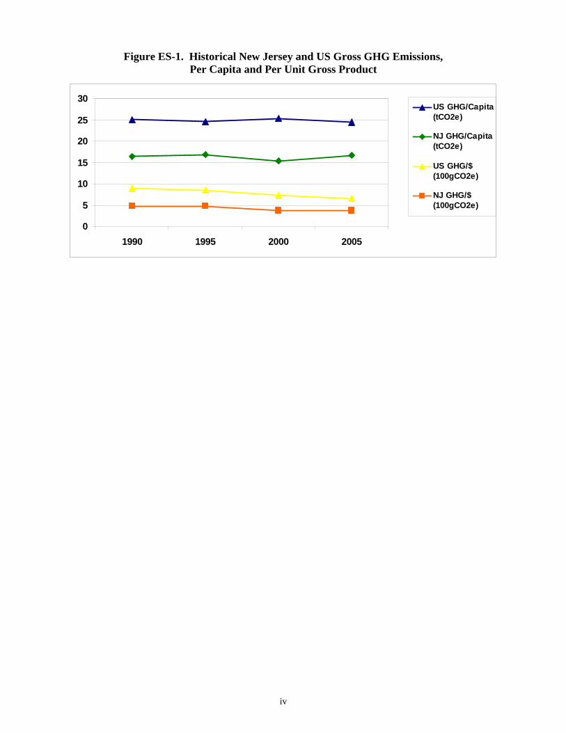
Figure ES-1 illustrates the State’s emissions per capita and per unit of economic output. On a per capita basis, New Jersey residents emitted about 16.9 metric tons (Mt) of gross CO2e in 1990, lower than the national average of 25.0 MtCO2e in 1990. Per capita emissions in New Jersey in 2005 were virtually unchanged from 1990, while the per capita emissions for the US decreased slightly to 24.5 MtCO2e/yr. As with the nation as a whole, economic growth exceeded emissions growth throughout the 1990-2005 period (leading to declining estimates of GHG emissions per unit of state product). From 1990 to 2005, emissions per unit of gross product dropped by 27% nationally, and by about 22% in New Jersey.3

There are three principal sources of GHG emissions in New Jersey: transportation; electricity consumption; and the residential, commercial, and industrial (RCI) fuel use sectors. Transportation accounted for 35% of New Jersey’s gross GHG emissions in 2005, while RCI fuel use accounted for 32% and electricity consumption contributed 24% of gross GHG emissions in 2005.

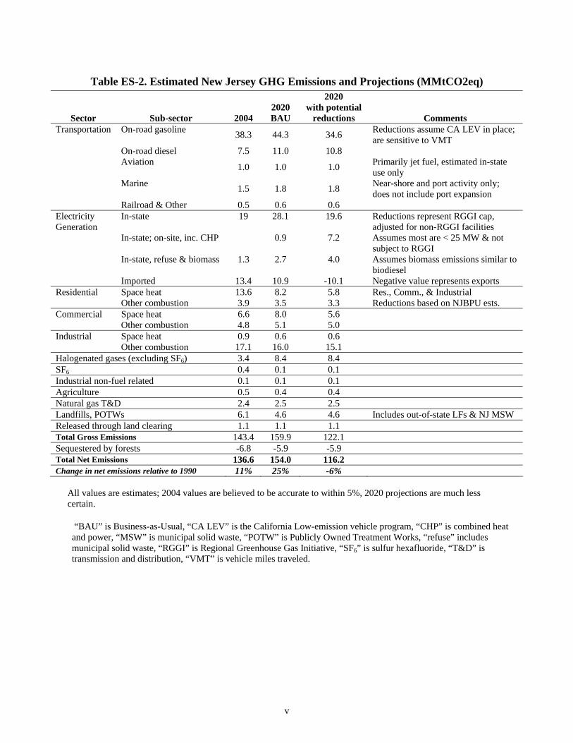
As shown in Table ES-1, New Jersey’s gross GHG emissions are projected to climb to about 159.9 MMTCO2eq by 2020, reaching 22% above 1990 levels. The transportation sector is projected to be the largest contributor to future emissions growth in New Jersey, followed by electricity consumption and substitutes for ozone-depleting substances (ODS) .

Some data gaps exist in this analysis, particularly for the reference case projections. Key refinements include review and revision of key emissions drivers that will be major determinants of New Jersey’s future GHG emissions (such as the growth rate assumptions for electricity generation and consumption, transportation fuel use, and RCI fuel use). Appendices A through H provide the detailed methods, data sources, and assumptions for each GHG sector. Also included are descriptions of significant uncertainties in emission estimates or methods and suggested next steps for refinement of the inventory.

Potential reductions Throughout this report, potential reductions in emissions are noted where it is anticipated that such reductions can be achieved with strategies consistent with the New Jersey Energy Master Plan, the Regional Greenhouse Gas Iniative (RGGI) and the California Low Emissions Vehicle Program as adopted by New Jersey. Although not factored into the estimates of potential reductions, recently enacted federal legislation4 will also have an effect on greenhouse gas emissions in the state.

3 Based on real gross domestic product (millions of chained 2000 dollars) that excludes the effects of inflation, available from the US Bureau of Economic Analysis (http://www.bea.gov/regional/gsp/). National emissions used for these comparisons are from http://www.epa.gov/climatechange/emissions/usinventoryreport.html. 4 The federal Energy Policy Act of 2007 requires refiners to use 9 billion gallons of grain ethanol in 2008 and 15 billion gallons annually by 2015. There also are separate new mandates for usage of biodiesel and fuels made from nonfood sources, such as crop waste and trees. The law also requires that by 2022 total biofuels use must reach 36 billion gallons annually."

iii

Table ES-1. New Jersey Historical and Reference Case GHG Emissions, by Sectora

(Million Metric Tons CO2e) 1990 2000 2005 2010 2020 Explanatory Notes for Projections Energy 111.9 118.4 130.4 131.2 145.1 Electricity, Production-Based 12.4 20.2 20.3 17.9 31.7 All electricity values based on NJBPU projections,

Coal 6.9 10.7 9.6 12.4 15.6 see assumptions in Appendix A. Natural Gas 3.6 7.4 8.3 4.1 13.4 Oil 1.7 0.9 1.1 0 0

Wood (CH4 and N2O) 0.01 0.03 0 0 0

Refuse and biomass 0.2 1.3 1.3 1.4 2.7 Under review; subject to revision

Net Imported Electricity 14.1 7.3 13.1 18.8 10.9

Electricity Consumption Based 26.5 27.5 33.4 36.7 42.6

Residential/Commercial/Industrial (RCI) 46.3 43.4 45.1 39.4 41.4

Coal 0.70 0.033 0.029 0.029 0.030 Based on USDOE data Natural Gas 20.5 25.6 26.2 22.9 26 Based on NJBPU projections Oil 25 17.7 18.8 16.4 15.3 Based on NJBPU projections and USDOE data Wood (CH4 and N2O) 0.14 0.09 0.08 0.08 0.08 Based on USDOE data

Transportation 36.6 45.2 49.5 52.7 58.6

On-road Gasoline 29.8 35.6 38.9 41.1 44.3 Based on USDOE regional projections

On-road Diesel 4.22 6.76 7.63 8.54 11.0 Based on USDOE regional projections Marine Vessels 1.01 1.35 1.48 1.56 1.79 Rail, Natural Gas, LPG, other 0.63 0.48 0.48 0.51 0.55 Based on USDOE regional projections Jet Fuel and Aviation Gasoline 1.00 1.00 1.00 1.00 1.00 Estimated in-state portion of emissions only Fossil Fuel Industry 2.5 2.2 2.4 2.5 2.6

Natural Gas Industry 2. 45 2.23 2.40 2.45 2.55

Industrial Processes 1.3 2.9 4.0 5.5 8.6

Nitric Acid Production (N2O) 0.203 0.001 0.001 0.001 0.001 Based on State's modeling forecast of manufacturing employment for 2006-2020

Limestone and Dolomite Use (CO2) 0.000 0.003 0.005 0.005 0.004 Based on State's modeling forecast of manufacturing

employment for 2006-2020

Soda Ash (CO2) 0.08 0.08 0.08 0.08 0.08 Based on 2004 and 2009 projections for U.S.

production ODS Substitutes (HFC, PFC) 0.010 2.41 3.59 5.16 8.37 EPA 2004 ODS cost study report

Electric Power T & D (SF6) 0.63 0.4 0.4 0.21 0.12 Based on national projections (USEPA)

Semiconductor Manufacturing (HFC, PFC, SF6)

0.01 0.03 0.03 0.02 0.01 Based on national projections (USEPA)

Laboratory Use of SF6 0.33 0.02 0.02 0.02 0.02 Assumed no change from 2005 levels.

Waste Management 15.9 7.8 5.9 5.1 4.6

Waste Combustion 0 0 0 0 0 Captured under electricity production sector

Landfills 15.4 7.3 5.4 4.5 4.0 Includes waste landfilled out of state

Wastewater Management 0.45 0.52 0.54 0.57 0.64 Projections based on historical 1990 to 2005 average annual growth rate.

Agriculture 0.6 0.6 0.5 0.5 0.4

Enteric Fermentation 0.13 0.09 0.08 0.07 0.06 Manure Management 0.04 0.03 0.03 0.03 0.02 Agricultural Soils 0.45 0.43 0.39 0.39 0.35

Forestry and Land Use (Land Clearing Releases) 1.1 1.1 1.1 1.1 1.1 Based on NJDEP methodology; See Appendix H

Total Gross Emissions 130.8 130.8 142.1 143.4 159.9 Forestry and Land Use (Sequestration) -7.5 -7.0 -6.7 -6.5 -5.9 Based on NJDEP methodology; See Appendix H Net Emissions (incl. forestry*) 123.2 123.8 135.3 136.9 154.0

Increase in net emissions relative to 1990 <1% 10% 11% 25% aAll values are estimates; 1990 and 2000 values are believed accurate to within 5%; projections are much less certain.

iv

Figure ES-1. Historical New Jersey and US Gross GHG Emissions, Per Capita and Per Unit Gross Product

0

5

10

15

20

25

30

1990 1995 2000 2005

US GHG/Capita(tCO2e)

NJ GHG/Capita(tCO2e)

US GHG/$(100gCO2e)

NJ GHG/$(100gCO2e)

v

Table ES-2. Estimated New Jersey GHG Emissions and Projections (MMtCO2eq)

Sector Sub-sector 2004 2020 BAU

2020 with potential

reductions Comments Transportation On-road gasoline 38.3 44.3 34.6 Reductions assume CA LEV in place;

are sensitive to VMT On-road diesel 7.5 11.0 10.8 Aviation 1.0 1.0 1.0 Primarily jet fuel, estimated in-state

use only Marine 1.5 1.8 1.8 Near-shore and port activity only;

does not include port expansion Railroad & Other 0.5 0.6 0.6 Electricity Generation

In-state 19 28.1 19.6 Reductions represent RGGI cap, adjusted for non-RGGI facilities

In-state; on-site, inc. CHP 0.9 7.2 Assumes most are < 25 MW & not subject to RGGI

In-state, refuse & biomass 1.3 2.7 4.0 Assumes biomass emissions similar to biodiesel

Imported 13.4 10.9 -10.1 Negative value represents exports Residential Space heat 13.6 8.2 5.8 Res., Comm., & Industrial Other combustion 3.9 3.5 3.3 Reductions based on NJBPU ests. Commercial Space heat 6.6 8.0 5.6 Other combustion 4.8 5.1 5.0 Industrial Space heat 0.9 0.6 0.6 Other combustion 17.1 16.0 15.1 Halogenated gases (excluding SF6) 3.4 8.4 8.4 SF6 0.4 0.1 0.1 Industrial non-fuel related 0.1 0.1 0.1 Agriculture 0.5 0.4 0.4 Natural gas T&D 2.4 2.5 2.5 Landfills, POTWs 6.1 4.6 4.6 Includes out-of-state LFs & NJ MSW Released through land clearing 1.1 1.1 1.1 Total Gross Emissions 143.4 159.9 122.1 Sequestered by forests -6.8 -5.9 -5.9 Total Net Emissions 136.6 154.0 116.2 Change in net emissions relative to 1990 11% 25% -6%

All values are estimates; 2004 values are believed to be accurate to within 5%, 2020 projections are much less certain. “BAU” is Business-as-Usual, “CA LEV” is the California Low-emission vehicle program, “CHP” is combined heat and power, “MSW” is municipal solid waste, “POTW” is Publicly Owned Treatment Works, “refuse” includes municipal solid waste, “RGGI” is Regional Greenhouse Gas Initiative, “SF6” is sulfur hexafluoride, “T&D” is transmission and distribution, “VMT” is vehicle miles traveled.

Table of Contents EXECUTIVE SUMMARY ........................................................................................................................................... I ACRONYMS AND KEY TERMS ...............................................................................................................................1 SUMMARY ..................................................................................................................................................................1 NEW JERSEY GREENHOUSE GAS EMISSIONS: SOURCES AND TRENDS.......................................................2

HISTORICAL EMISSIONS.............................................................................................................................................4 Overview ..............................................................................................................................................................4

A CLOSER LOOK AT THE THREE MAJOR SOURCES: TRANSPORTATION, RCI FUEL USE SECTOR, AND ELECTRICITY SUPPLY......................................................................................................................................................................5

Transportation Sector ..........................................................................................................................................5 Residential, Commercial, and Industrial (RCI) Sector ........................................................................................6 Electricity Supply Sector ......................................................................................................................................6

REFERENCE CASE PROJECTIONS (BUSINESS AS USUAL) ............................................................................................7 POTENTIAL REDUCTIONS ...........................................................................................................................................7 KEY UNCERTAINTIES AND NEXT STEPS.....................................................................................................................9 APPROACH.................................................................................................................................................................9 GENERAL METHODOLOGY.......................................................................................................................................10 GENERAL PRINCIPLES AND GUIDELINES..................................................................................................................10

• Transparency............................................................................................................................................10 • Consistency: .............................................................................................................................................10 • Priority of Existing State and Local Data Sources...................................................................................10 • Priority of Significant Emissions Sources ................................................................................................11 • Comprehensive Coverage of Gases, Sectors, State Activities, and Time Periods. ...................................11 • Use of Consumption-Based Emissions Estimates:....................................................................................11

APPENDIX A. ENERGY SUPPLY............................................................................................................................14 APPENDIX B. RESIDENTIAL, COMMERCIAL, AND INDUSTRIAL (RCI) FUEL COMBUSTION .................21 APPENDIX C. TRANSPORTATION ENERGY USE...............................................................................................27 APPENDIX D. INDUSTRIAL PROCESSES.............................................................................................................38 APPENDIX E. FOSSIL FUEL EXTRACTION AND DISTRIBUTION INDUSTRY ..............................................48 APPENDIX F. AGRICULTURE ................................................................................................................................51 APPENDIX G. WASTE MANAGEMENT ................................................................................................................58 APPENDIX H. FORESTRY AND LAND-USE CHANGE .......................................................................................64 APPENDIX I. RESPONSES TO COMMENTS ON DRAFT INVENTORY ............................................................68

Table of Tables Table ES-1. New Jersey Historical and Reference Case GHG Emissions, by Sectora................. iii Table ES-2. Estimated New Jersey GHG Emissions and Projections (MMtCO2eq)..................... v Table 1. New Jersey Historical and Reference Case GHG Emissions, by Sectora........................ 3 Table 2. Estimated New Jersey GHG Emissions and Projections (MMtCO2eq) ........................... 8 Table 3. Key Annual Growth Rates for New Jersey, Historical and Projected ............................. 9 Table 4. Key Sources for New Jersey Data, Inventory Methods, and Growth Rates.................. 12 Table A1. Electricity Sales to Meet New Jersey Demand ........................................................... 16 Table B1a. Residential Sector Emissions Inventory and Reference Case Projections (MMtCO2e)

........................................................................................................................................... 24 Table B2b. Residential Sector Proportions of Total Emissions by Fuel Type (%) ...................... 24

Table B2a. Commercial Sector Emissions Inventory and Reference Case Projections (MMtCO2e) ....................................................................................................................... 25

Table B2b. Commercial Sector Proportions of Total Emissions by Fuel Type (%) .................... 25 Table B3a. Industrial Sector Emissions Inventory and................................................................. 25 Reference Case Projections (MMtCO2e) ...................................................................................... 25 Table B3b. Industrial Sector Proportions of Total Emissions by Fuel Type (%) ......................... 26 Table C1. Key Assumptions and Methods for the Transportation Inventory and Projections ..... 28 Table C2. New Jersey Projected Vehicle Miles Traveled Estimates (millions) ........................... 29 Table C3. New Jersey Vehicle Miles Traveled Compound Annual Growth Rates...................... 30 Table C4. New Jersey On-road Fuel Consumption Compound Annual Growth Rates................ 30 Table C5. New Jersey Compound Annual Growth Rates for Marine Fuels................................. 31 Table C6. Summary of New Jersey GHG Marine Emissions....................................................... 32 Table C7. New Jersey Aviation Fuels Compound Annual Growth Rates.................................... 33 Table C8. Summary of New Jersey Aviation GHG Emissions .................................................... 34 Table C9. EIA Classification of Gasoline and Diesel Consumption ............................................ 34 Table C10. Summary of New Jersey GHG Emissions and Reference Case Projections ............. 35 Table C11. Summary of New Jersey GHG Emissions and Reference Case Projections ............. 36 Table D1. Approach to Estimating Historical Emissions ............................................................. 39 Table D1. Approach to Estimating Historical Emissions (Continued)......................................... 40 Table D2. Approach to Estimating Projections ............................................................................ 40 Table D2. Approach to Estimating Projections (Continued) ........................................................ 41 Table D3. Historic and Projected Emissions for the Industrial Processes Sector (MMtCO2e) ... 42 Table E1. Approach to Estimating Historical and Future Methane Emissions from Natural Gas

Transmission and Distribution.......................................................................................... 49 Table E2. Emissions Inventory and Reference Case Projections (MMtCO2e)............................ 50 Table E2. Proportions of Total Subsector Emissions by Type and Source (%) .......................... 50 Table F1. Growth Rates Applied for the Enteric Fermentation.................................................... 53 and Manure Management Categories ........................................................................................... 53 Table F2. Growth Rates Applied for the Agricultural Sector....................................................... 53 Table F3. GHG Emissions from Soil Carbon Changes Due to Cultivation Practices (MMtCO2e)

........................................................................................................................................... 54 Table F4. Net GHG Emissions from Agriculture (MMtCO2eq).................................................. 56 Table G1. Controlled Solid Waste Landfills................................................................................ 59 Table G2. SGIT Key Default Values for Municipal Wastewater Treatment ............................... 61 Table G3. New Jersey GHG Emissions from Waste Management (MMtCO2eq)........................ 62 Table H1. New Jersey Land-Use Type, Acres, from NJDEP/GIS .............................................. 65 Table H2. New Jersey Land-Use Type, Acres, from CRSSA ..................................................... 65 Table H3. Method 1 Estimated CO2 Equivalent Sequestration, New Jersey............................... 66 Table H4. Resultant Estimated CO2 Equivalent Sequestration, New Jersey............................... 67 Table of Figures

Figure 1. Historical New Jersey and US Gross GHG Emissions, Per Capita and Per Unit Gross

Product ................................................................................................................................ 4 Figure A1. Electricity Generation to Meet New Jersey Demand (GWh/Year) ........................... 15 Figure A2. New Jersey In-State Generation by Fuel (1990-2005) .............................................. 18

Figure C1. New Jersey Transportation GHG Emissions by Sector, 1990-2020........................... 35 Figure D1. Non-combustion GHG Emissions from Industrial Processes, 1990-2020 ................ 42 Figure D2. Non-combustion GHG Emissions from Industrial Processes, 1990-2020, by Source

........................................................................................................................................... 43 Figure F1. Gross GHG Emissions from Agriculture ................................................................... 56

Acronyms and Key Terms

AEO2006 – EIA’s Annual Energy Outlook 2006

Ag – Agriculture

BAU – Business as Usual

bbls – Barrels

BC – Black Carbon

Bcf – Billion cubic feet

BOD – Biochemical Oxygen Demand

BTU – British thermal unit

C – Carbon

CaCO3 – Calcium Carbonate

CCS – Center for Climate Strategies

CEC – Commission for Environmental Cooperation

CEEEP – Center for Energy, Economic & Environmental Policy (Rutgers University)

CFCs – Chlorofluorocarbons

CH4 – Methane

CO – Carbon Monoxide

CO2 – Carbon Dioxide

CO2eq – Carbon Dioxide equivalent

COLE – Carbon Online Estimator

CRP – Federal Conservation Reserve Program

CRSSA – Center for Remote Sensing and Spatial Analysis

EC – Elemental Carbon

EEZ – Exclusive Economic Zone

EIA – US DOE Energy Information Administration

EIIP – Emissions Inventory Improvement Program

EMP – Energy Master Plan

FAA – Federal Aviation Administration

FAPRI – Food and Agricultural Policy Research Institute

FHWA – Federal Highway Administration

FIA – Forest Inventory Analysis

GHG – Greenhouse Gases

GIS – Geographical Information System

GWh – Gigawatt-hour

GWP – Global Warming Potential

HFCs – Hydrofluorocarbons

IPCC – Intergovernmental Panel on Climate Change

kWh – kilowatt-hour

LandGEM – Landfill Gas Emissions Model

lb – pound

LF – Landfill

LFGTE – Landfill Gas Collection System and Landfill-Gas-to-Energy

LNG – Liquified Natural Gas

LPG – Liquified Petroleum Gas

MMBtu – Million British thermal units

MMt – Million Metric tons

MMTCO2eq – Million Metric tons Carbon Dioxide equivalent

Mt – Metric ton (equivalent to 1.102 short tons)

MSW – Municipal Solid Waste

MW – Megawatt

MWh – Megawatt-hour

N – Nitrogen

N2O – Nitrous Oxide

NEI – National Emissions Inventory

NO2 – Nitrogen Dioxide

NOx – Nitrogen Oxides

NASS – National Agricultural Statistics Service

NJDEP – New Jersey Department of Environmental Protection

NJDOT – New Jersey Department of Transportation

NMVOCs – Nonmethane Volatile Organic Compounds

O3 – Ozone

ODS – Ozone-Depleting Substances

OM – Organic Matter

PFCs – Perfluorocarbons

PM – Particulate Matter

POTW – Publicly Owned Treatment Works

ppb – parts per billion

ppm – parts per million

ppt – parts per trillion

RCI – Residential, Commercial, and Industrial

RGGI – Regional Greenhouse Gas Initiative

RPS – Renewable Portfolio Standard

SAR – Second Assessment Report

SED – State Energy Data

SF6 – Sulfur Hexafluoride

SGIT – State Greenhouse Gas Inventory Tool

Sinks – Removals of carbon from the atmosphere, with the carbon stored in forests, soils, landfills, wood structures, or other biomass-related products.

TAR – Third Assessment Report

T&D – Transmission and Distribution

TBtu – Trillion British Thermal Units

TOG – Total Organic Carbon

UNFCCC – United Nations Framework Convention on Climate Change

US EPA – United States Environmental Protection Agency

US DOE – United States Department of Energy

USDA – United States Department of Agriculture

USFS – United States Forest Service

USGS – United States Geological Survey

VMT – Vehicle-Miles Traveled

W/m2 – Watts per Square Meter

WMO – World Meteorological Organization

WW – Wastewater

yr – year

.

1

Summary

This report was prepared in response to directives of Governor Corzine’s Executive Order 54 and the New Jersey Global Warming Response Act. This report presents a preliminary inventory and forecast of the State’s greenhouse gas (GHG) emissions from 1990 to 2020. The inventory and forecast estimates serve as a starting point to assist the State with an initial comprehensive understanding of New Jersey’s current and possible future GHG emissions, and thereby inform the identification and analysis of policy options for mitigating GHG emissions. The Global Warming Response Act directs DEP to evaluate and recommend such policy options.

A draft of this report was posted on the New Jersey Global Warming website (http://www.state.nj.us/globalwarming/index.shtml) in February, 2008. Numerous comments and recommendations were received. The DEP has reviewed these comments and has made several improvements to the inventory and forecasts as a result. A summary of the most significant comments and the DEP’s responses are presented in Appendix I of this report. The BPU, in its Energy Master Plan (http://www.nj.gov/emp), has provided updates to the energy use data and projections that were used to estimate some of the GHG emissions in the February, 2008 draft report. These most recent data and projections have been used in preparing this report. New Jersey’s anthropogenic GHG emissions and anthropogenic sinks (carbon storage) were estimated for the period from 1990 to 2020. Historical GHG emission estimates (1990 through 2005)5 were developed using a set of generally accepted principles and guidelines for State GHG emissions inventories, as described in the “Approach” section below, relying to the extent possible on New Jersey-specific data and inputs. The initial reference case projections (2006-2020) are based on a compilation of various existing projections of electricity generation, fuel use, and other GHG-emitting activities, along with a set of simple, transparent assumptions described in the appendices of this report.

This report covers the six gases included in the US Greenhouse Gas Inventory: carbon dioxide (CO2), methane (CH4), nitrous oxide (N2O), hydrofluorocarbons (HFCs), perfluorocarbons (PFCs), and sulfur hexafluoride (SF6). Emissions of these GHGs are presented using a common metric, CO2 equivalence (CO2eq), which indicates the relative contribution of each gas to global average radiative forcing on a Global Warming Potential- (GWP) weighted basis.

It is important to note that the preliminary emissions estimates reflect the GHG emissions associated with the electricity sources used to meet New Jersey’s demands, corresponding to a consumption-based approach to emissions accounting (see “Approach” section below). Another way to look at electricity emissions is to consider the GHG emissions produced by electricity generation facilities in the State. This report covers both methods of accounting for emissions, but for consistency, all total results are reported as consumption-based.

5 The last year of available historical data varies by sector; ranging from 2000 to 2006.

2

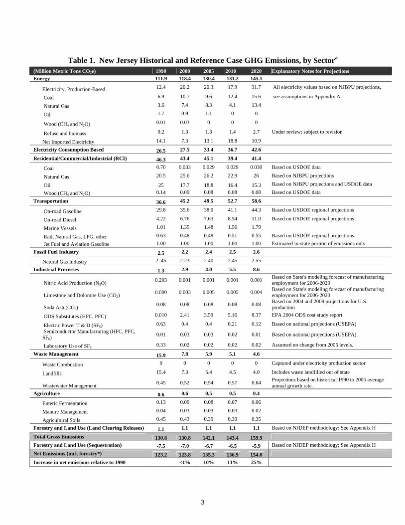
New Jersey Greenhouse Gas Emissions: Sources and Trends Table 1 provides a summary of GHG emissions estimated for New Jersey by sector for the years 1990, 2000, 2005, 2010, and 2020. Details on the methods and data sources used to construct these draft estimates are provided in the appendices to this report. In the sections below, we discuss GHG emission sources (positive, or gross, emissions) and sinks (negative emissions) separately in order to identify trends, projections, and uncertainties clearly for each. This next section of the report provides a summary of the historical emissions (1990 through 2005) followed by a summary of the reference-case projection-year emissions (2006 through 2020) and key uncertainties. We also provide an overview of the general methodology, principles, and guidelines followed for preparing the inventories. Appendices A through H provide the detailed methods, data sources, and assumptions for each GHG sector.

3

Table 1. New Jersey Historical and Reference Case GHG Emissions, by Sectora

(Million Metric Tons CO2e) 1990 2000 2005 2010 2020 Explanatory Notes for Projections Energy 111.9 118.4 130.4 131.2 145.1 Electricity, Production-Based 12.4 20.2 20.3 17.9 31.7 All electricity values based on NJBPU projections,

Coal 6.9 10.7 9.6 12.4 15.6 see assumptions in Appendix A. Natural Gas 3.6 7.4 8.3 4.1 13.4 Oil 1.7 0.9 1.1 0 0

Wood (CH4 and N2O) 0.01 0.03 0 0 0

Refuse and biomass 0.2 1.3 1.3 1.4 2.7 Under review; subject to revision

Net Imported Electricity 14.1 7.3 13.1 18.8 10.9

Electricity Consumption Based 26.5 27.5 33.4 36.7 42.6

Residential/Commercial/Industrial (RCI) 46.3 43.4 45.1 39.4 41.4

Coal 0.70 0.033 0.029 0.029 0.030 Based on USDOE data Natural Gas 20.5 25.6 26.2 22.9 26 Based on NJBPU projections Oil 25 17.7 18.8 16.4 15.3 Based on NJBPU projections and USDOE data Wood (CH4 and N2O) 0.14 0.09 0.08 0.08 0.08 Based on USDOE data

Transportation 36.6 45.2 49.5 52.7 58.6

On-road Gasoline 29.8 35.6 38.9 41.1 44.3 Based on USDOE regional projections

On-road Diesel 4.22 6.76 7.63 8.54 11.0 Based on USDOE regional projections Marine Vessels 1.01 1.35 1.48 1.56 1.79 Rail, Natural Gas, LPG, other 0.63 0.48 0.48 0.51 0.55 Based on USDOE regional projections Jet Fuel and Aviation Gasoline 1.00 1.00 1.00 1.00 1.00 Estimated in-state portion of emissions only Fossil Fuel Industry 2.5 2.2 2.4 2.5 2.6

Natural Gas Industry 2. 45 2.23 2.40 2.45 2.55

Industrial Processes 1.3 2.9 4.0 5.5 8.6

Nitric Acid Production (N2O) 0.203 0.001 0.001 0.001 0.001 Based on State's modeling forecast of manufacturing employment for 2006-2020

Limestone and Dolomite Use (CO2) 0.000 0.003 0.005 0.005 0.004 Based on State's modeling forecast of manufacturing

employment for 2006-2020

Soda Ash (CO2) 0.08 0.08 0.08 0.08 0.08 Based on 2004 and 2009 projections for U.S.

production ODS Substitutes (HFC, PFC) 0.010 2.41 3.59 5.16 8.37 EPA 2004 ODS cost study report

Electric Power T & D (SF6) 0.63 0.4 0.4 0.21 0.12 Based on national projections (USEPA)

Semiconductor Manufacturing (HFC, PFC, SF6)

0.01 0.03 0.03 0.02 0.01 Based on national projections (USEPA)

Laboratory Use of SF6 0.33 0.02 0.02 0.02 0.02 Assumed no change from 2005 levels.

Waste Management 15.9 7.8 5.9 5.1 4.6

Waste Combustion 0 0 0 0 0 Captured under electricity production sector

Landfills 15.4 7.3 5.4 4.5 4.0 Includes waste landfilled out of state

Wastewater Management 0.45 0.52 0.54 0.57 0.64 Projections based on historical 1990 to 2005 average annual growth rate.

Agriculture 0.6 0.6 0.5 0.5 0.4

Enteric Fermentation 0.13 0.09 0.08 0.07 0.06 Manure Management 0.04 0.03 0.03 0.03 0.02 Agricultural Soils 0.45 0.43 0.39 0.39 0.35

Forestry and Land Use (Land Clearing Releases) 1.1 1.1 1.1 1.1 1.1 Based on NJDEP methodology; See Appendix H

Total Gross Emissions 130.8 130.8 142.1 143.4 159.9 Forestry and Land Use (Sequestration) -7.5 -7.0 -6.7 -6.5 -5.9 Based on NJDEP methodology; See Appendix H Net Emissions (incl. forestry*) 123.2 123.8 135.3 136.9 154.0

Increase in net emissions relative to 1990 <1% 10% 11% 25%

4

aAll values are estimates; 1990 and 2000 values are believed accurate to within 5%; projections are much less certain.

Historical Emissions

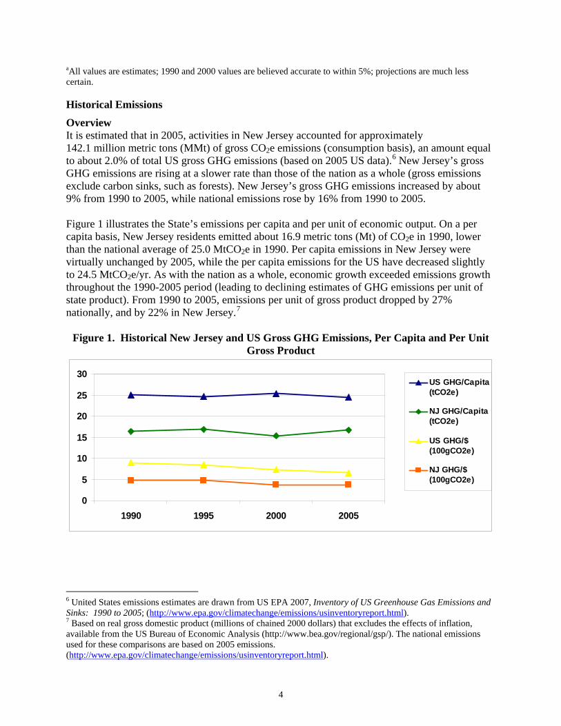
Overview It is estimated that in 2005, activities in New Jersey accounted for approximately 142.1 million metric tons (MMt) of gross CO2e emissions (consumption basis), an amount equal to about 2.0% of total US gross GHG emissions (based on 2005 US data).6 New Jersey’s gross GHG emissions are rising at a slower rate than those of the nation as a whole (gross emissions exclude carbon sinks, such as forests). New Jersey’s gross GHG emissions increased by about 9% from 1990 to 2005, while national emissions rose by 16% from 1990 to 2005. Figure 1 illustrates the State’s emissions per capita and per unit of economic output. On a per capita basis, New Jersey residents emitted about 16.9 metric tons (Mt) of CO2e in 1990, lower than the national average of 25.0 MtCO2e in 1990. Per capita emissions in New Jersey were virtually unchanged by 2005, while the per capita emissions for the US have decreased slightly to 24.5 MtCO2e/yr. As with the nation as a whole, economic growth exceeded emissions growth throughout the 1990-2005 period (leading to declining estimates of GHG emissions per unit of state product). From 1990 to 2005, emissions per unit of gross product dropped by 27% nationally, and by 22% in New Jersey.7

Figure 1. Historical New Jersey and US Gross GHG Emissions, Per Capita and Per Unit Gross Product

0

5

10

15

20

25

30

1990 1995 2000 2005

US GHG/Capita(tCO2e)

NJ GHG/Capita(tCO2e)

US GHG/$(100gCO2e)

NJ GHG/$(100gCO2e)

6 United States emissions estimates are drawn from US EPA 2007, Inventory of US Greenhouse Gas Emissions and Sinks: 1990 to 2005; (http://www.epa.gov/climatechange/emissions/usinventoryreport.html). 7 Based on real gross domestic product (millions of chained 2000 dollars) that excludes the effects of inflation, available from the US Bureau of Economic Analysis (http://www.bea.gov/regional/gsp/). The national emissions used for these comparisons are based on 2005 emissions. (http://www.epa.gov/climatechange/emissions/usinventoryreport.html).

5

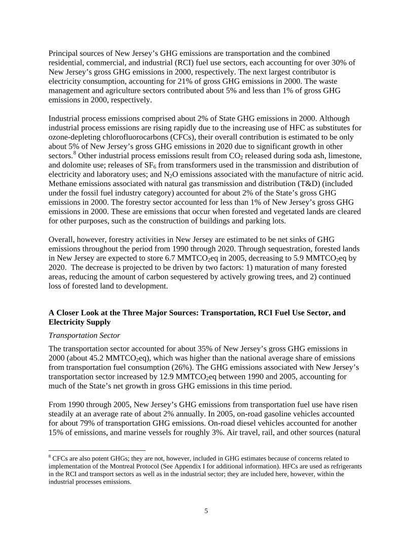
Principal sources of New Jersey’s GHG emissions are transportation and the combined residential, commercial, and industrial (RCI) fuel use sectors, each accounting for over 30% of New Jersey’s gross GHG emissions in 2000, respectively. The next largest contributor is electricity consumption, accounting for 21% of gross GHG emissions in 2000. The waste management and agriculture sectors contributed about 5% and less than 1% of gross GHG emissions in 2000, respectively. Industrial process emissions comprised about 2% of State GHG emissions in 2000. Although industrial process emissions are rising rapidly due to the increasing use of HFC as substitutes for ozone-depleting chlorofluorocarbons (CFCs), their overall contribution is estimated to be only about 5% of New Jersey’s gross GHG emissions in 2020 due to significant growth in other sectors.8 Other industrial process emissions result from CO2 released during soda ash, limestone, and dolomite use; releases of SF6 from transformers used in the transmission and distribution of electricity and laboratory uses; and N2O emissions associated with the manufacture of nitric acid. Methane emissions associated with natural gas transmission and distribution (T&D) (included under the fossil fuel industry category) accounted for about 2% of the State’s gross GHG emissions in 2000. The forestry sector accounted for less than 1% of New Jersey’s gross GHG emissions in 2000. These are emissions that occur when forested and vegetated lands are cleared for other purposes, such as the construction of buildings and parking lots. Overall, however, forestry activities in New Jersey are estimated to be net sinks of GHG emissions throughout the period from 1990 through 2020. Through sequestration, forested lands in New Jersey are expected to store 6.7 MMTCO2eq in 2005, decreasing to 5.9 MMTCO2eq by 2020. The decrease is projected to be driven by two factors: 1) maturation of many forested areas, reducing the amount of carbon sequestered by actively growing trees, and 2) continued loss of forested land to development.

A Closer Look at the Three Major Sources: Transportation, RCI Fuel Use Sector, and Electricity Supply

Transportation Sector

The transportation sector accounted for about 35% of New Jersey’s gross GHG emissions in 2000 (about 45.2 MMTCO2eq), which was higher than the national average share of emissions from transportation fuel consumption (26%). The GHG emissions associated with New Jersey’s transportation sector increased by 12.9 MMTCO2eq between 1990 and 2005, accounting for much of the State’s net growth in gross GHG emissions in this time period. From 1990 through 2005, New Jersey’s GHG emissions from transportation fuel use have risen steadily at an average rate of about 2% annually. In 2005, on-road gasoline vehicles accounted for about 79% of transportation GHG emissions. On-road diesel vehicles accounted for another 15% of emissions, and marine vessels for roughly 3%. Air travel, rail, and other sources (natural

8 CFCs are also potent GHGs; they are not, however, included in GHG estimates because of concerns related to implementation of the Montreal Protocol (See Appendix I for additional information). HFCs are used as refrigerants in the RCI and transport sectors as well as in the industrial sector; they are included here, however, within the industrial processes emissions.

6

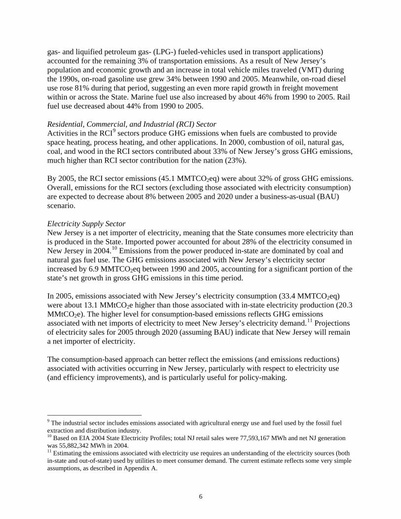
gas- and liquified petroleum gas- (LPG-) fueled-vehicles used in transport applications) accounted for the remaining 3% of transportation emissions. As a result of New Jersey’s population and economic growth and an increase in total vehicle miles traveled (VMT) during the 1990s, on-road gasoline use grew 34% between 1990 and 2005. Meanwhile, on-road diesel use rose 81% during that period, suggesting an even more rapid growth in freight movement within or across the State. Marine fuel use also increased by about 46% from 1990 to 2005. Rail fuel use decreased about 44% from 1990 to 2005. Residential, Commercial, and Industrial (RCI) Sector Activities in the RCI9 sectors produce GHG emissions when fuels are combusted to provide space heating, process heating, and other applications. In 2000, combustion of oil, natural gas, coal, and wood in the RCI sectors contributed about 33% of New Jersey’s gross GHG emissions, much higher than RCI sector contribution for the nation (23%).

By 2005, the RCI sector emissions (45.1 MMTCO2eq) were about 32% of gross GHG emissions. Overall, emissions for the RCI sectors (excluding those associated with electricity consumption) are expected to decrease about 8% between 2005 and 2020 under a business-as-usual (BAU) scenario. Electricity Supply Sector New Jersey is a net importer of electricity, meaning that the State consumes more electricity than is produced in the State. Imported power accounted for about 28% of the electricity consumed in New Jersey in 2004.10 Emissions from the power produced in-state are dominated by coal and natural gas fuel use. The GHG emissions associated with New Jersey’s electricity sector increased by 6.9 MMTCO2eq between 1990 and 2005, accounting for a significant portion of the state’s net growth in gross GHG emissions in this time period. In 2005, emissions associated with New Jersey’s electricity consumption (33.4 MMTCO2eq) were about 13.1 MMtCO2e higher than those associated with in-state electricity production (20.3 MMtCO2e). The higher level for consumption-based emissions reflects GHG emissions associated with net imports of electricity to meet New Jersey’s electricity demand.11 Projections of electricity sales for 2005 through 2020 (assuming BAU) indicate that New Jersey will remain a net importer of electricity. The consumption-based approach can better reflect the emissions (and emissions reductions) associated with activities occurring in New Jersey, particularly with respect to electricity use (and efficiency improvements), and is particularly useful for policy-making.

9 The industrial sector includes emissions associated with agricultural energy use and fuel used by the fossil fuel extraction and distribution industry. 10 Based on EIA 2004 State Electricity Profiles; total NJ retail sales were 77,593,167 MWh and net NJ generation was 55,882,342 MWh in 2004. 11 Estimating the emissions associated with electricity use requires an understanding of the electricity sources (both in-state and out-of-state) used by utilities to meet consumer demand. The current estimate reflects some very simple assumptions, as described in Appendix A.

7

Reference Case Projections (Business as Usual) Relying on a variety of sources for projections, as noted below and in the appendices, we developed a simple reference case projection of GHG emissions through 2020. As shown numerically in Table 1, under the reference case projections, New Jersey’s gross GHG emissions continue to grow steadily, climbing to about 159.9 MMtCO2e by 2020, 22% above 1990 levels. The transportation sector is projected to be the largest contributor to future emissions growth, followed by emissions associated with electricity consumption and then by ODS Substitutes (HFCs). Table 2 provides a sector-level summary of emissions for 2004 (the latest year for which activity data were available), 2020 BAU, and 2020 with potential reductions.

Potential reductions Throughout this report, potential reductions in emissions are noted where it is anticipated that such reductions can be achieved with strategies consistent with the New Jersey Energy Master Plan,12 the Regional Greenhouse Gas Initiative (RGGI),13 and the California Low Emissions Vehicle Program as adopted by New Jersey. Although not factored into the estimates of potential reductions, recently enacted federal legislation14 will also have an effect on greenhouse gas emissions in the state.

12 See http://www.nj.gov/emp 13 See http://www.rggi.org/home 14 The federal Energy Policy Act of 2007 requires refiners to use 9 billion gallons of grain ethanol in 2008 and 15 billion gallons annually by 2015. There also are separate new mandates for usage of biodiesel and fuels made from nonfood sources, such as crop waste and trees. The law also requires that by 2022 total biofuels use must reach 36 billion gallons annually."

8

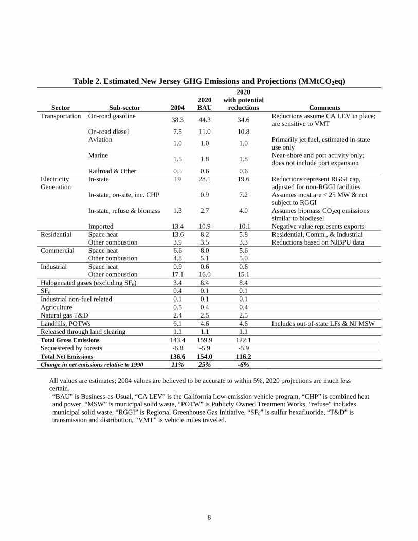
Table 2. Estimated New Jersey GHG Emissions and Projections (MMtCO2eq)

Sector Sub-sector 2004 2020 BAU

2020 with potential

reductions Comments Transportation On-road gasoline 38.3 44.3 34.6 Reductions assume CA LEV in place;

are sensitive to VMT On-road diesel 7.5 11.0 10.8 Aviation 1.0 1.0 1.0 Primarily jet fuel, estimated in-state

use only Marine 1.5 1.8 1.8 Near-shore and port activity only;

does not include port expansion Railroad & Other 0.5 0.6 0.6 Electricity Generation

In-state 19 28.1 19.6 Reductions represent RGGI cap, adjusted for non-RGGI facilities

In-state; on-site, inc. CHP 0.9 7.2 Assumes most are < 25 MW & not subject to RGGI

In-state, refuse & biomass 1.3 2.7 4.0 Assumes biomass CO2eq emissions similar to biodiesel

Imported 13.4 10.9 -10.1 Negative value represents exports Residential Space heat 13.6 8.2 5.8 Residential, Comm., & Industrial Other combustion 3.9 3.5 3.3 Reductions based on NJBPU data Commercial Space heat 6.6 8.0 5.6 Other combustion 4.8 5.1 5.0 Industrial Space heat 0.9 0.6 0.6 Other combustion 17.1 16.0 15.1 Halogenated gases (excluding SF6) 3.4 8.4 8.4 SF6 0.4 0.1 0.1 Industrial non-fuel related 0.1 0.1 0.1 Agriculture 0.5 0.4 0.4 Natural gas T&D 2.4 2.5 2.5 Landfills, POTWs 6.1 4.6 4.6 Includes out-of-state LFs & NJ MSW Released through land clearing 1.1 1.1 1.1 Total Gross Emissions 143.4 159.9 122.1 Sequestered by forests -6.8 -5.9 -5.9 Total Net Emissions 136.6 154.0 116.2 Change in net emissions relative to 1990 11% 25% -6%

All values are estimates; 2004 values are believed to be accurate to within 5%, 2020 projections are much less certain. “BAU” is Business-as-Usual, “CA LEV” is the California Low-emission vehicle program, “CHP” is combined heat and power, “MSW” is municipal solid waste, “POTW” is Publicly Owned Treatment Works, “refuse” includes municipal solid waste, “RGGI” is Regional Greenhouse Gas Initiative, “SF6” is sulfur hexafluoride, “T&D” is transmission and distribution, “VMT” is vehicle miles traveled.

9

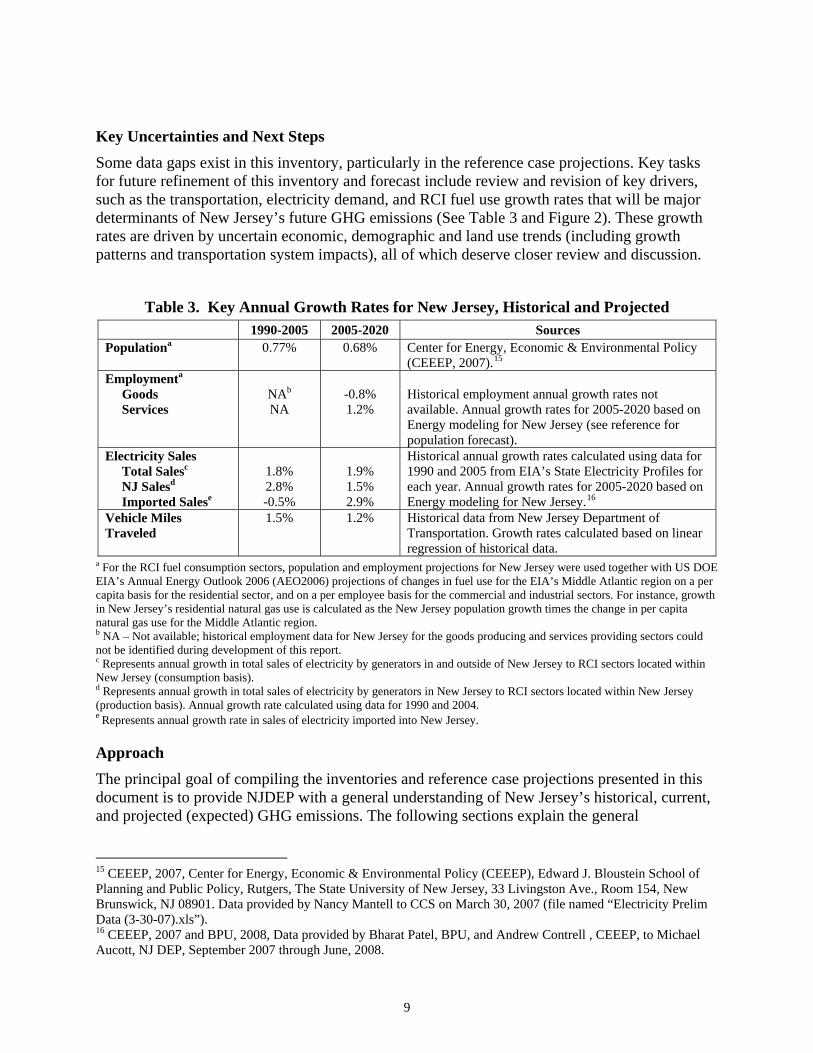
Key Uncertainties and Next Steps Some data gaps exist in this inventory, particularly in the reference case projections. Key tasks for future refinement of this inventory and forecast include review and revision of key drivers, such as the transportation, electricity demand, and RCI fuel use growth rates that will be major determinants of New Jersey’s future GHG emissions (See Table 3 and Figure 2). These growth rates are driven by uncertain economic, demographic and land use trends (including growth patterns and transportation system impacts), all of which deserve closer review and discussion.

Table 3. Key Annual Growth Rates for New Jersey, Historical and Projected 1990-2005 2005-2020 Sources

Populationa 0.77% 0.68% Center for Energy, Economic & Environmental Policy (CEEEP, 2007).15

Employmenta Goods Services

NAb NA

-0.8% 1.2%

Historical employment annual growth rates not available. Annual growth rates for 2005-2020 based on Energy modeling for New Jersey (see reference for population forecast).

Electricity Sales Total Salesc NJ Salesd

Imported Salese

1.8% 2.8% -0.5%

1.9% 1.5% 2.9%

Historical annual growth rates calculated using data for 1990 and 2005 from EIA’s State Electricity Profiles for each year. Annual growth rates for 2005-2020 based on Energy modeling for New Jersey.16

Vehicle Miles Traveled

1.5% 1.2% Historical data from New Jersey Department of Transportation. Growth rates calculated based on linear regression of historical data.

a For the RCI fuel consumption sectors, population and employment projections for New Jersey were used together with US DOE EIA’s Annual Energy Outlook 2006 (AEO2006) projections of changes in fuel use for the EIA’s Middle Atlantic region on a per capita basis for the residential sector, and on a per employee basis for the commercial and industrial sectors. For instance, growth in New Jersey’s residential natural gas use is calculated as the New Jersey population growth times the change in per capita natural gas use for the Middle Atlantic region. b NA – Not available; historical employment data for New Jersey for the goods producing and services providing sectors could not be identified during development of this report. c Represents annual growth in total sales of electricity by generators in and outside of New Jersey to RCI sectors located within New Jersey (consumption basis). d Represents annual growth in total sales of electricity by generators in New Jersey to RCI sectors located within New Jersey (production basis). Annual growth rate calculated using data for 1990 and 2004. e Represents annual growth rate in sales of electricity imported into New Jersey.

Approach The principal goal of compiling the inventories and reference case projections presented in this document is to provide NJDEP with a general understanding of New Jersey’s historical, current, and projected (expected) GHG emissions. The following sections explain the general

15 CEEEP, 2007, Center for Energy, Economic & Environmental Policy (CEEEP), Edward J. Bloustein School of Planning and Public Policy, Rutgers, The State University of New Jersey, 33 Livingston Ave., Room 154, New Brunswick, NJ 08901. Data provided by Nancy Mantell to CCS on March 30, 2007 (file named “Electricity Prelim Data (3-30-07).xls”). 16 CEEEP, 2007 and BPU, 2008, Data provided by Bharat Patel, BPU, and Andrew Contrell , CEEEP, to Michael Aucott, NJ DEP, September 2007 through June, 2008.

10

methodology and the general principles and guidelines followed during development of these GHG inventories for New Jersey.

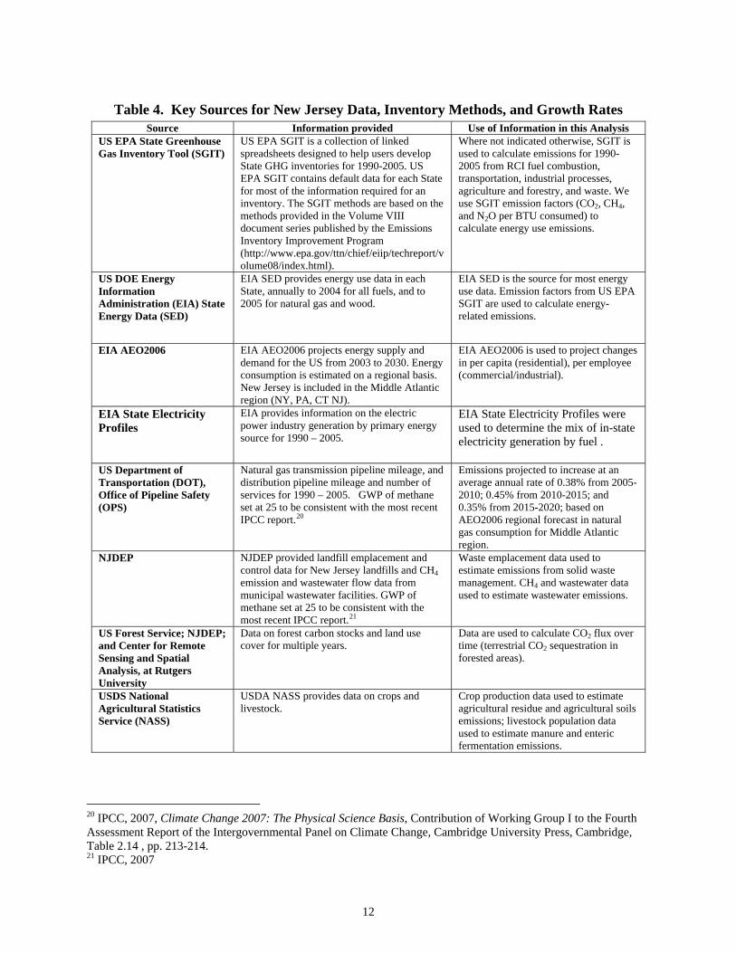
General Methodology The analyses contained in this report were developed in consultation with other state agencies, most notably, the Board of Public Utilities, and in conference with The Center for Climate Strategies, The Rutgers University, Center for Energy, Economic and Environmental Policy and stakeholders. The overall goal of this effort is to provide simple and straightforward estimates, with an emphasis on robustness, consistency, and transparency. As a result, we rely on reference forecasts from best available State and regional sources where possible. Where reliable existing forecasts are lacking, we use straightforward spreadsheet analysis and constant growth-rate extrapolations of historical trends rather than complex modeling. In most cases, we follow the same approach to emissions accounting for historical inventories used by the US EPA in its national GHG emissions inventory17 and its guidelines for States.18 These inventory guidelines were developed based on the guidelines from the Intergovernmental Panel on Climate Change (IPCC), the international organization responsible for developing coordinated methods for national GHG inventories.19 The inventory methods provide flexibility to account for local conditions. The key sources of activity and projection data used are shown in Table 4. Table 4 also provides the descriptions of the data provided by each source and the uses of each data set in this analysis.

General Principles and Guidelines A key part of this effort involves the establishment and use of a set of generally accepted accounting principles for evaluation of historical and projected GHG emissions, as follows:

• Transparency: We report data sources, methods, and key assumptions to allow open review and opportunities for additional revisions later based on input from others. In addition, we will report key uncertainties where they exist.

• Consistency: To the extent possible, the inventory and projections will be designed to be externally consistent with current or likely future systems for State and national GHG emission reporting. We have used the EPA tools for State inventories and projections as a starting point. These initial estimates were then augmented and/or revised as needed to conform with State-based inventory and base-case projection needs. For consistency in making reference case projections, we define reference case actions for the purposes of projections as those currently in place or reasonably expected over the time period of analysis.

• Priority of Existing State and Local Data Sources: In gathering data and in cases where data sources conflicted, we placed highest priority on local and State data and

17 US EPA 2007, Inventory of US Greenhouse Gas Emissions and Sinks: 1990 to 2005; (http://www.epa.gov/climatechange/emissions/usinventoryreport.html).. 18 http://yosemite.epa.gov/oar/globalwarming.nsf/content/EmissionsStateInventoryGuidance.html. 19 http://www.ipcc-nggip.iges.or.jp/public/gl/invs1.htm.

11

analyses, followed by regional sources, with national data or simplified assumptions such as constant linear extrapolation of trends used as defaults where necessary.

• Priority of Significant Emissions Sources: In general, activities with relatively small emissions levels may not be reported with the same level of detail as other activities.

• Comprehensive Coverage of Gases, Sectors, State Activities, and Time Periods. This analysis aims to comprehensively cover GHG emissions associated with activities in New Jersey. It covers all six GHGs covered by US and other national inventories: CO2, CH4, N2O, SF6, HFCs, and PFCs. The inventory estimates are for the year 1990, with subsequent years included up to most recently available data (typically 2002 to 2005), with projections to 2010 and 2020.

• Use of Consumption-Based Emissions Estimates: To the extent possible, we estimated emissions that are caused by activities that occur in New Jersey. For example, we reported emissions associated with the electricity consumed in New Jersey. The rationale for this method of reporting is that it can more accurately reflect the impact of State-based policy strategies such as energy efficiency on overall GHG emissions, and it resolves double-counting and exclusion problems with multi-emissions issues. This approach can differ from how inventories are compiled, for example, on an in-state production basis, in particular for electricity.

12

Table 4. Key Sources for New Jersey Data, Inventory Methods, and Growth Rates Source Information provided Use of Information in this Analysis

US EPA State Greenhouse Gas Inventory Tool (SGIT)

US EPA SGIT is a collection of linked spreadsheets designed to help users develop State GHG inventories for 1990-2005. US EPA SGIT contains default data for each State for most of the information required for an inventory. The SGIT methods are based on the methods provided in the Volume VIII document series published by the Emissions Inventory Improvement Program (http://www.epa.gov/ttn/chief/eiip/techreport/volume08/index.html).

Where not indicated otherwise, SGIT is used to calculate emissions for 1990-2005 from RCI fuel combustion, transportation, industrial processes, agriculture and forestry, and waste. We use SGIT emission factors (CO2, CH4, and N2O per BTU consumed) to calculate energy use emissions.

US DOE Energy Information Administration (EIA) State Energy Data (SED)

EIA SED provides energy use data in each State, annually to 2004 for all fuels, and to 2005 for natural gas and wood.

EIA SED is the source for most energy use data. Emission factors from US EPA SGIT are used to calculate energy-related emissions.

EIA AEO2006

EIA AEO2006 projects energy supply and demand for the US from 2003 to 2030. Energy consumption is estimated on a regional basis. New Jersey is included in the Middle Atlantic region (NY, PA, CT NJ).

EIA AEO2006 is used to project changes in per capita (residential), per employee (commercial/industrial).

EIA State Electricity Profiles

EIA provides information on the electric power industry generation by primary energy source for 1990 – 2005.

EIA State Electricity Profiles were used to determine the mix of in-state electricity generation by fuel .

US Department of Transportation (DOT), Office of Pipeline Safety (OPS)

Natural gas transmission pipeline mileage, and distribution pipeline mileage and number of services for 1990 – 2005. GWP of methane set at 25 to be consistent with the most recent IPCC report.20

Emissions projected to increase at an average annual rate of 0.38% from 2005-2010; 0.45% from 2010-2015; and 0.35% from 2015-2020; based on AEO2006 regional forecast in natural gas consumption for Middle Atlantic region.

NJDEP NJDEP provided landfill emplacement and control data for New Jersey landfills and CH4 emission and wastewater flow data from municipal wastewater facilities. GWP of methane set at 25 to be consistent with the most recent IPCC report.21

Waste emplacement data used to estimate emissions from solid waste management. CH4 and wastewater data used to estimate wastewater emissions.

US Forest Service; NJDEP; and Center for Remote Sensing and Spatial Analysis, at Rutgers University

Data on forest carbon stocks and land use cover for multiple years.

Data are used to calculate CO2 flux over time (terrestrial CO2 sequestration in forested areas).

USDS National Agricultural Statistics Service (NASS)

USDA NASS provides data on crops and livestock.

Crop production data used to estimate agricultural residue and agricultural soils emissions; livestock population data used to estimate manure and enteric fermentation emissions.

20 IPCC, 2007, Climate Change 2007: The Physical Science Basis, Contribution of Working Group I to the Fourth Assessment Report of the Intergovernmental Panel on Climate Change, Cambridge University Press, Cambridge, Table 2.14 , pp. 213-214. 21 IPCC, 2007

13

For electricity, we estimate, in addition to the emissions due to fuels combusted at electricity plants in the State, the emissions related to electricity consumed in New Jersey. This entails accounting for the electricity sources used by New Jersey utilities to meet consumer demands. As this analysis is refined in the future, one could also attempt to estimate other sectoral emissions on a consumption basis, such as accounting for emissions from transportation fuel used in New Jersey, but purchased out-of-state. In some cases, this can require venturing into the relatively complex terrain of life-cycle analysis. In general, we recommend considering a consumption-based approach where it will significantly improve the estimation of the emissions impact of potential mitigation strategies. For example re-use, recycling, and source reduction can lead to emission reductions resulting from lower energy requirements for material production (such as paper, cardboard, and aluminum), even though production of those materials, and emissions associated with materials production, may not occur within the State. Details on the methods and data sources used to construct the inventories and forecasts for each source sector are provided in the following appendices:

• Appendix A. Electricity Use and Supply • Appendix B. Residential, Commercial, and Industrial (RCI) Fuel Combustion • Appendix C. Transportation Energy Use • Appendix D. Industrial Processes • Appendix E. Fossil Fuel Extraction and Distribution Industry • Appendix F. Agriculture • Appendix G. Waste Management • Appendix H. Forestry

14

Appendix A. Energy Supply Overview This appendix describes the data sources, key assumptions, and the methodology used to develop an inventory of greenhouse gas (GHG) emissions over the 1990-2004 period associated with the generation of electricity to meet electricity demand in New Jersey. It also describes the data sources, key assumptions, and methodology used to develop a forecast of GHG emissions over the 2005-2020 period associated with meeting future electricity demand in the state under a “business-as-usual (BAU)” scenario. Emissions (Business-as-Usual)

Total New Jersey Demand for Electricity

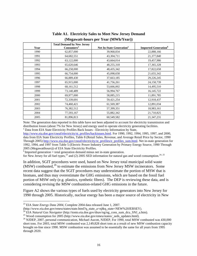
Figure A1 shows the historical trend in retail sales of electricity to the RCI sectors in New Jersey for 1990 through 2005. Overall, total retail sales of electricity for all sectors increased by an average annual rate of 1.8% from 1990 to 2005, and by 3.2% from 2000 to 2005. From 1990 through 2005, residential and commercial sales have increased at about the same average annual rate (i.e., 2.6% and 2.5%, respectively) while average annual sales of electricity for the industrial sector have declined slightly (-1.6%). Table A1 shows the values used to develop Figure A1. Table A1 also shows electricity sales from in-state generators of electricity as well as sales of imported electricity to meet New Jersey’s electricity demand.

In-State Generation of Electricity

Emissions associated with the generation of electricity by electricity generating units in New Jersey were estimated using the March 2007 release of the United States Environmental Protection Agency’s (US EPA) State Greenhouse Gas Inventory Tool (SGIT) software and the methods provided in the Emission Inventory Improvement Program (EIIP) guidance document for fuel combustion.22 The default data used in SGIT for New Jersey are from the United States Department of Energy (US DOE) Energy Information Administration’s (EIA) State Energy Data (SED) for 1990 through 2003. The SGIT files were updated to include (1) 2004 SED information

22 GHG emissions were calculated using SGIT, with reference to EIIP, Volume VIII: Chapter 1 “Methods for Estimating Carbon Dioxide Emissions from Combustion of Fossil Fuels”, August 2004, and Chapter 2 “Methods for Estimating Methane and Nitrous Oxide Emissions from Stationary Combustion”, August 2004. The March 2007 versions of the SGIT Excel files (CO2FFC Module.xls and Stationary Combustion Module.xls) containing SED through 2003 for all fuels and sectors were used as the starting point for preparing the inventory for New Jersey.

15

Figure A1. Electricity Generation to Meet New Jersey Demand (GWh/Year)

0

10,000

20,000

30,000

40,000

50,000

60,000

70,000

80,000

90,000

1990

1991

1992

1993

1994

1995

1996

1997

1998

1999

2000

2001

2002

2003

2004

2005

GW

h

Residential Industrial Commercial + Other All Sectors

16

Table A1. Electricity Sales to Meet New Jersey Demand (Megawatt-hours per Year (MWh/Year))

Year Total Demand by New Jersey

Consumersa Net In-State Generationa Imported Generationb 1990 62,857,000 39,968,834 22,888,166 1991 64,682,551 43,304,711 21,377,840 1992 63,122,000 43,664,014 19,457,986 1993 65,620,646 48,255,318 17,365,328 1994 66,258,000 48,435,342 17,822,658 1995 66,754,000 45,098,658 21,655,342 1996 66,889,430 37,663,185 29,226,245 1997 65,915,000 41,756,261 24,158,739 1998 68,161,512 53,666,002 14,495,510 1999 73,140,489 56,994,767 16,145,722 2000 69,977,000 58,085,215 11,891,785 2001 72,339,691 59,421,254 12,918,437 2002 74,460,421 61,569,387 12,891,034 2003 76,382,512 57,399,351 18,983,161 2004 77,593,167 55,882,342 21,710,825 2005 81,896,813 60,549,582 21,347,231

Note: The generation data reported in this table have not been adjusted to account for electricity transmission and distribution losses (about 7% for New Jersey) and energy used to operate electricity generating facilities. a Data from EIA State Electricity Profiles Back Issues - Electricity Information by State, http://www.eia.doe.gov/cneaf/electricity/st_profiles/backissues.html. For 1990, 1992, 1994, 1995, 1997, and 2000, data from EIA State Electricity Profiles, Table 8 (Retail Sales, Revenue, and Average Retail Price by Sector, 1990 Through 2005) http://www.eia.doe.gov/cneaf/electricity/st_profiles/e_profiles_sum.html. Net in-state generation for 1992, 1994, and 1997 from Table 5 (Electric Power Industry Generation by Primary Energy Source, 1990 Through 2005 (Megawatthours)) of EIA State Electricity Profiles. b Imported generation = total generation demand minus net in-state generation. for New Jersey for all fuel types,23 and (2) 2005 SED information for natural gas and wood consumption.24, 25

In addition, SGIT procedures were used, based on New Jersey total municipal solid waste (MSW) combusted,26 to estimate the emissions from New Jersey MSW incinerators. Some recent data suggest that the SGIT procedures may underestimate the portion of MSW that is biomass, and thus may overestimate the GHG emissions, which are based on the fossil fuel portion of MSW only (e.g. plastics, synthetic fibres). The DEP is reviewing these data, and is considering revising the MSW combustion-related GHG emissions in the future.

Figure A2 shows the various types of fuels used by electricity generators into New Jersey for 1990 through 2005. Historically, nuclear energy has been a major source of electricity in New 23 EIA State Energy Data 2004, Complete 2004 data released June 1, 2007. (http://www.eia.doe.gov/emeu/states/state.html?q_state_a=nj&q_state=NEW%20JERSEY). 24 EIA Natural Gas Navigator (http://tonto.eia.doe.gov/dnav/ng/ng_cons_sum_dcu_SNJ_a.htm). 25 Wood consumption for 2005 (http://www.eia.doe.gov/emeu/states/_seds_updates.html). 26 NJDEP, 2007, personal communication, Michael Aucott, NJDEP, For 1990, total MSW combusted was 430,000 short tons. For 2003, total MSW combusted was 2,149,828 short tons as a result of new MSW combustion capacity brought on-line since 1990. MSW combustion was assumed to be essentially the same for all years from 1995 through 2020.

17

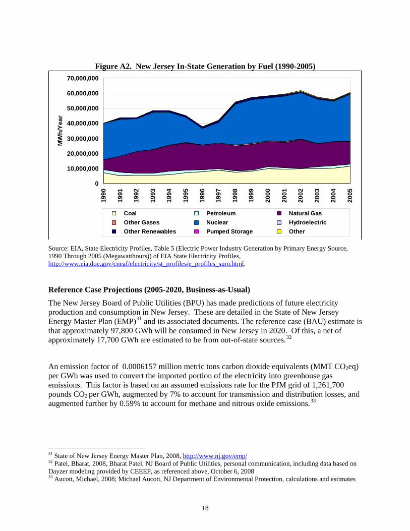
Jersey, followed by natural gas, coal, and petroleum. Electricity generated from nuclear fuel varied significantly from 1990 through 2005, ranging from a low of 29% in 1996 to a high of 59% in 1990. From 2000 through 2005, electricity generated from nuclear fuel remained fairly stable in New Jersey’s total fuel mix ranging from 48% to 52% over this six-year period.

Electricity generated from natural gas also varied significantly from 1990 through 2005, ranging from a low of 17% in 1990 to a high of 44% in 1996. From 2000 through 2005, electricity generated from natural gas ranged from 25% to 31% of New Jersey’s total fuel mix. Electricity generated from coal from 1990 through 2005 ranged from a low of 11% in 1993 to a high of 21% in 1996 and 1997. From 2000 through 2005, electricity generated from coal ranged from 16% to 19% of New Jersey’s total fuel mix. Sales of electricity generated from natural gas and coal peaked from 1995 through 1997 offsetting a decline in sales associated with electricity generated from nuclear fuel during this period. Electricity generated from petroleum from 1990 through 2005 ranged from a low of 1% in 1998, 1999, and 2002 to a high of 5% in 1990 and 1991. From 2000 through 2005, electricity generated from petroleum ranged from 1% to 3% of New Jersey’s total fuel mix. Other fuel resources that have been used to generate electricity in New Jersey include industrial gases, landfill gas, MSW, and a small amount of hydroelectric power and pumped storage energy.

Imported Electricity

Emissions associated with the generation of electricity that is imported to New Jersey were estimated using data from the EIA State Electricity Profiles.27 The calculation took the total retail electricity sales from the Profiles and subtracted from it the net in-state generation, as also reported in the Profiles (see Table A1). The difference was then multiplied by the factor of 1,261.7 pounds (lbs) CO2 per Megawatt-hour (MWh),28 and then augmented with an additional 7% to account for transmission and distribution (T&D) losses.29 The resulting quantity was further augmented by multiplying by the factor of 1.006304 to represent additional emissions of CH4 and N2O.30

27 EIA State Electricity Profiles 2004, May 2006, and earlier editions, from Energy Information Administration, Office of Coal, Nuclear and Alternate Fuels, U.S. Department of Energy, Washington, DC 20585-0650, http://www.eia.doe.gov/cneaf/electricity/st_profiles/e_profiles_sum.html, accessed September, 2007 28 CEEEP, 2007, Based on emissions rate of the PJM power control area, the primary source of imported electricity in NJ, as reported by Center for Energy, Economic & Environmental Policy (CEEEP), Edward J. Bloustein School of Planning and Public Policy, Rutgers, The State University of New Jersey, 33 Livingston Ave., Room 154, New Brunswick, NJ 08901, June, 2007. 29 As estimated by Bill Doughtery, CCS, personal communication, July 19, 2007, and Julia Hutchins, U.S. DOE EIA, personal communication, July, 2007. 30 This value was developed by M. Aucott, NJDEP, using the factors of 6 x 10-1 metric tons N2O per trillion British thermal unit (TBtu) and 10.02 metric tons CH4 per TBtu for all fuels except natural gas, 0.09 x 10-1 metric tons N2O per TBtu and 4.75 metric tons CH4 per TBtu for natural gas, 310 and 25 for the global warming potential of these two gases, respectively, as weighted based on estimated fuel mix of the PJM generation facilities being 15% natural gas with the rest of the fossil fuel being oil and coal.

18

Figure A2. New Jersey In-State Generation by Fuel (1990-2005)

0

10,000,000

20,000,000

30,000,000

40,000,000

50,000,000

60,000,000

70,000,000

1990

1991

1992

1993

1994

1995

1996

1997

1998

1999

2000

2001

2002

2003

2004

2005

MW

h/Ye

ar

Coal Petroleum Natural Gas Other Gases Nuclear Hydroelectric Other Renewables Pumped Storage Other

Source: EIA, State Electricity Profiles, Table 5 (Electric Power Industry Generation by Primary Energy Source, 1990 Through 2005 (Megawatthours)) of EIA State Electricity Profiles, http://www.eia.doe.gov/cneaf/electricity/st_profiles/e_profiles_sum.html.

Reference Case Projections (2005-2020, Business-as-Usual) The New Jersey Board of Public Utilities (BPU) has made predictions of future electricity production and consumption in New Jersey. These are detailed in the State of New Jersey Energy Master Plan (EMP)31 and its associated documents. The reference case (BAU) estimate is that approximately 97,800 GWh will be consumed in New Jersey in 2020. Of this, a net of approximately 17,700 GWh are estimated to be from out-of-state sources.32

An emission factor of 0.0006157 million metric tons carbon dioxide equivalents (MMT CO2eq) per GWh was used to convert the imported portion of the electricity into greenhouse gas emissions. This factor is based on an assumed emissions rate for the PJM grid of 1,261,700 pounds CO2 per GWh, augmented by 7% to account for transmission and distribution losses, and augmented further by 0.59% to account for methane and nitrous oxide emissions.33

31 State of New Jersey Energy Master Plan, 2008, http://www.nj.gov/emp/ 32 Patel, Bharat, 2008, Bharat Patel, NJ Board of Public Utilities, personal communication, including data based on Dayzer modeling provided by CEEEP, as referenced above, October 6, 2008 33 Aucott, Michael, 2008; Michael Aucott, NJ Department of Environmental Protection, calculations and estimates

19

The total BAU CO2eq emissions for electricity generation in 2020 are estimated to be 31.7 MMT from in-state generation facilities, including 2.7 MMT from MSW resource recovery (MSW incineration) facilities and biomass combustion, and 10.9 MMT from the production of net imported electricity. BAU values for 2010 are expected to be 17.8 MMT from in-state generation facilities, including 1.4 MMT from MSW resource recovery (MSW incineration) facilities and biomass combustion, and 18.8MMT from the production of net imported electricity.34

Alternate Case Projections

The EMP includes a wide variety of measures that are expected to achieve an overall reduction of 20% or more of energy use below the business-as-usual value by 2020. These measures include the development of on-shore and off-shore wind generation capacity, addition of more photovoltaic electricity generation capacity, importation of more electricity derived from renewable sources, more use of biomass, additional energy-conserving appliance standards, new, energy-conserving building codes, and the installation of a variety of energy-saving measures at existing buildings. The EMP also expects to facilitate the addition of a significant amount of new generation in the form of combined heat and power facilities, which also produce usable heat energy, which will reduce the need to obtain this heat from combustion of fuels. The specific reductions projected to result from these measures are not detailed herein. See the EMP website as referenced above for more details.

The results of these overall reductions are depicted in Table ES-2 and Table 2 above. These tables show, in the “2020 with potential reductions” column, that the implementation of these measures as planned leads to a significant reduction of electricity use and its associated emission (and also results in reductions of emissions from direct fuel use by the residential, commercial, and industrial sectors.)_ If the emissions reductions associated with reduced use of electricity are all subtracted from the reference case imported electricity emissions estimate, the emissions from imported electricity drop to a negative value. A reduction this large would potentially enable New Jersey in-state facilities to export power.

These tables also show an estimated emission from in-state facilities of 19.6 MMT. This value represents the portion of the overall RGGI cap that is accounted for by RGGI facilities, plus the emissions of those in-state generation facilities that are not subject to the RGGI program.35 The RGGI program does not in actuality have state-specific caps. However, if New Jersey facilities do not operate up to the level of their assumed capacity as allowed by the overall RGGI cap because of the energy use reduction measures implemented through the EMP (or for other reasons) facilities in other states would be able to emit proportionately more and still stay within the overall RGGI cap.. For this reason, the in-state emission is assumed to be equal to the portion of the RGGI cap that applies to NJ facilities.

34 Patel, Bharat, 2008, as referenced above. 35 The RGGI cap effective as of 2020 is assumed to be 10% below the 2006 estimated emission from NJ’s RGGI facilities (20.6 MMT), which translates to a cap of 18.7 MMT. This emissions quantity is likely to be augmented by approximately 5%, representing emissions from facilities not subject to the RGGI cap, bringing the total to approximately 19.6 MMT.

20

It is important to note, however, that the interrelationship of RGGI limits and projected exported electricity, and the resulting CO2eq emissions, cannot be estimated with precision without knowing the state to which that electricity is exported and the fuel mix of the sources involved, both of which are quite uncertain at this time. It is also important to note that the various projections described above, and elsewhere in this report, are essentially based on extrapolation, through a variety of methods, of existing trends. But trends are not destiny. Projections of energy use and greenhouse gas emissions into the future carry major uncertainties. A variety of factors, including percent utilization of New Jersey’s nuclear generation capacity vs. its fossil-based generation capacity, cost of fuels and other economic influences, political events, and the emergence of new technologies, could significantly alter future scenarios.

21

Appendix B. Residential, Commercial, and Industrial (RCI) Fuel Combustion Overview Activities in the residential, commercial, and industrial (RCI)36 sectors produce carbon dioxide (CO2), methane (CH4), and nitrous oxide (N2O) emissions when fuels are combusted to provide space heating, water heating, process heating, cooking, and other energy end-uses. Carbon dioxide accounts for over 99% of these emissions on a million metric tons (MMt) of CO2 equivalent (CO2e) basis in New Jersey. Direct use of oil, natural gas, coal, and wood in the RCI sectors accounted for an estimated 45.1 MMtCO2eq of gross greenhouse gas (GHG) emissions in 2005.37 The following discusses the data sources, methods, assumptions, and results used to construct the inventory (1990 to most recent year for which fuel use data are available (i.e., 2004 or 2005)), and reference case projections (2004 or 2005 to 2020) based on business-as-usual assumptions. Emissions and Reference Case Projections (Business-as-Usual) Emissions for the years 1990, 1995, 2000, and 2004 from direct fuel use were estimated using the March 2007 release of the United States Environmental Protection Agency’s (US EPA) State Greenhouse Gas Inventory Tool (SGIT) software and the methods provided in the Emission Inventory Improvement Program (EIIP) guidance document for RCI fuel combustion.38 The default data used in SGIT for New Jersey are from the United States Department of Energy (US DOE) Energy Information Administration’s (EIA) State Energy Data (SED) for 1990 through 2003. The SGIT files were updated to include (1) 2004 SED information for New Jersey for all fuel types for each of the RCI sectors,39 and (2) 2005 SED information for natural gas and wood consumption.40, 41 Note that the EIIP methods for the industrial sector exclude from CO2 emission estimates the amount of carbon that is stored in products produced from fossil fuels for non-energy uses. For example, the methods account for carbon stored in petrochemical feedstocks, and in liquefied petroleum gases (LPG) and natural gas used as feedstocks by chemical manufacturing plants (i.e., not used as fuel), as well as carbon stored in asphalt and road oil produced from petroleum.

36 The industrial sector includes emissions associated with agricultural energy use and fuel used by natural gas transmission and distribution (T&D) industry. 37 Emissions estimates from wood combustion include only N2O and CH4. Carbon dioxide emissions from biomass combustion are assumed to be “net zero”, consistent with US EPA and Intergovernmental Panel on Climate Change (IPCC) methodologies, and any net loss of carbon stocks due to biomass fuel use should be accounted for in the land use and forestry analysis. 38 GHG emissions were calculated using SGIT, with reference to EIIP, Volume VIII: Chapter 1 “Methods for Estimating Carbon Dioxide Emissions from Combustion of Fossil Fuels”, August 2004, and Chapter 2 “Methods for Estimating Methane and Nitrous Oxide Emissions from Stationary Combustion”, August 2004. The March 2007 versions of the SGIT Excel files (CO2FFC Module.xls and Stationary Combustion Module.xls) containing SED through 2003 for all fuels and sectors were used as the starting point for preparing the inventory for New Jersey. 39 EIA State Energy Data 2004, Complete 2004 data released June 1, 2007. (http://www.eia.doe.gov/emeu/states/state.html?q_state_a=nj&q_state=NEW%20JERSEY). 40 EIA Natural Gas Navigator (http://tonto.eia.doe.gov/dnav/ng/ng_cons_sum_dcu_SNJ_a.htm). 41 RCI wood consumption for 2005 (http://www.eia.doe.gov/emeu/states/_seds_updates.html).

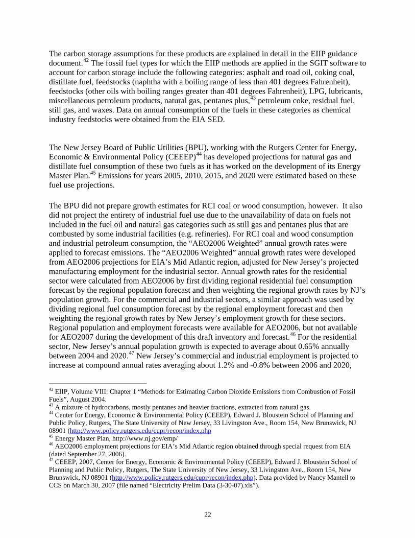
22

The carbon storage assumptions for these products are explained in detail in the EIIP guidance document.42 The fossil fuel types for which the EIIP methods are applied in the SGIT software to account for carbon storage include the following categories: asphalt and road oil, coking coal, distillate fuel, feedstocks (naphtha with a boiling range of less than 401 degrees Fahrenheit), feedstocks (other oils with boiling ranges greater than 401 degrees Fahrenheit), LPG, lubricants, miscellaneous petroleum products, natural gas, pentanes plus,43 petroleum coke, residual fuel, still gas, and waxes. Data on annual consumption of the fuels in these categories as chemical industry feedstocks were obtained from the EIA SED. The New Jersey Board of Public Utilities (BPU), working with the Rutgers Center for Energy, Economic & Environmental Policy (CEEEP)44 has developed projections for natural gas and distillate fuel consumption of these two fuels as it has worked on the development of its Energy Master Plan.45 Emissions for years 2005, 2010, 2015, and 2020 were estimated based on these fuel use projections. The BPU did not prepare growth estimates for RCI coal or wood consumption, however. It also did not project the entirety of industrial fuel use due to the unavailability of data on fuels not included in the fuel oil and natural gas categories such as still gas and pentanes plus that are combusted by some industrial facilities (e.g. refineries). For RCI coal and wood consumption and industrial petroleum consumption, the “AEO2006 Weighted” annual growth rates were applied to forecast emissions. The “AEO2006 Weighted” annual growth rates were developed from AEO2006 projections for EIA’s Mid Atlantic region, adjusted for New Jersey’s projected manufacturing employment for the industrial sector. Annual growth rates for the residential sector were calculated from AEO2006 by first dividing regional residential fuel consumption forecast by the regional population forecast and then weighting the regional growth rates by NJ’s population growth. For the commercial and industrial sectors, a similar approach was used by dividing regional fuel consumption forecast by the regional employment forecast and then weighting the regional growth rates by New Jersey’s employment growth for these sectors. Regional population and employment forecasts were available for AEO2006, but not available for AEO2007 during the development of this draft inventory and forecast.46 For the residential sector, New Jersey’s annual population growth is expected to average about 0.65% annually between 2004 and 2020.47 New Jersey’s commercial and industrial employment is projected to increase at compound annual rates averaging about 1.2% and -0.8% between 2006 and 2020,

42 EIIP, Volume VIII: Chapter 1 “Methods for Estimating Carbon Dioxide Emissions from Combustion of Fossil Fuels”, August 2004. 43 A mixture of hydrocarbons, mostly pentanes and heavier fractions, extracted from natural gas. 44 Center for Energy, Economic & Environmental Policy (CEEEP), Edward J. Bloustein School of Planning and Public Policy, Rutgers, The State University of New Jersey, 33 Livingston Ave., Room 154, New Brunswick, NJ 08901 (http://www.policy.rutgers.edu/cupr/recon/index.php 45 Energy Master Plan, http://www.nj.gov/emp/ 46 AEO2006 employment projections for EIA’s Mid Atlantic region obtained through special request from EIA (dated September 27, 2006). 47 CEEEP, 2007, Center for Energy, Economic & Environmental Policy (CEEEP), Edward J. Bloustein School of Planning and Public Policy, Rutgers, The State University of New Jersey, 33 Livingston Ave., Room 154, New Brunswick, NJ 08901 (http://www.policy.rutgers.edu/cupr/recon/index.php). Data provided by Nancy Mantell to CCS on March 30, 2007 (file named “Electricity Prelim Data (3-30-07).xls”).

23

respectively.48 Wood and coal combustion represent relatively tiny portions of the total emissions for these sectors. Results Residential Sector

For the residential sector, emissions from direct fossil fuel use in 1990 were about 15.7 MMtCO2eq, and are estimated to decrease to about 11.5 MMtCO2e by 2020. Emissions associated with natural gas consumption accounted for about 60% of total residential emissions in 1990, and are estimated to increase to 98% of total residential emissions by 2020. In 1990, petroleum consumption accounted for about 40% of total residential emissions, and is estimated to account for about 24% of total residential emissions by 2020. Residential-sector emissions associated with the use of coal and wood in 1990 were about 0.12 MMtCO2eq combined, and accounted for about 0.8% of total residential emissions. By 2020, emissions associated with the consumption of these two fuels are estimated to fall to 0.06 MMtCO2eq, accounting for 0.3% of total residential sector emissions by that year. Coal consumption by the residential sector has been and is expected to continue to be negligible from 1990 through 2020.

48 CEEEP, 2007, Center for Energy, Economic & Environmental Policy (CEEEP), Edward J. Bloustein School of Planning and Public Policy, Rutgers, The State University of New Jersey, 33 Livingston Ave., Room 154, New Brunswick, NJ 08901 (http://www.policy.rutgers.edu/cupr/recon/index.php). Data provided by Nancy Mantell to CCS on March 30, 2007 (file named “Electricity Prelim Data (3-30-07).xls”).

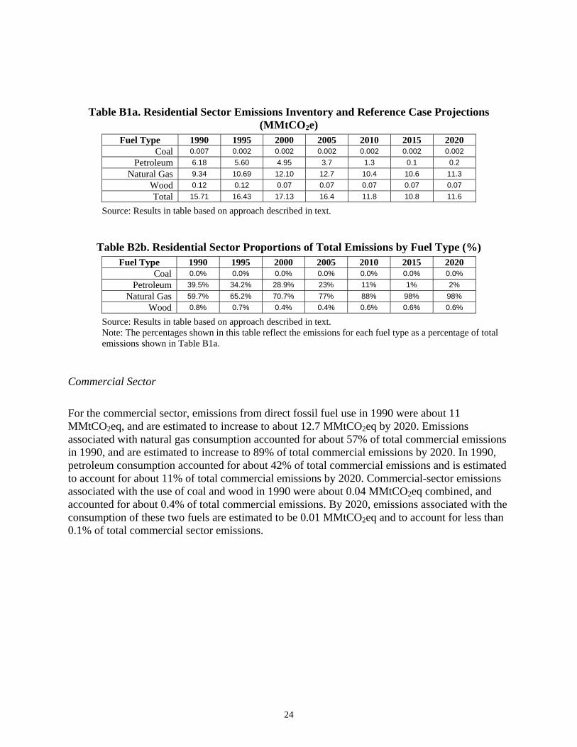
24

Table B1a. Residential Sector Emissions Inventory and Reference Case Projections (MMtCO2e)

Fuel Type 1990 1995 2000 2005 2010 2015 2020 Coal 0.007 0.002 0.002 0.002 0.002 0.002 0.002

Petroleum 6.18 5.60 4.95 3.7 1.3 0.1 0.2 Natural Gas 9.34 10.69 12.10 12.7 10.4 10.6 11.3

Wood 0.12 0.12 0.07 0.07 0.07 0.07 0.07 Total 15.71 16.43 17.13 16.4 11.8 10.8 11.6

Source: Results in table based on approach described in text.

Table B2b. Residential Sector Proportions of Total Emissions by Fuel Type (%) Fuel Type 1990 1995 2000 2005 2010 2015 2020

Coal 0.0% 0.0% 0.0% 0.0% 0.0% 0.0% 0.0% Petroleum 39.5% 34.2% 28.9% 23% 11% 1% 2%

Natural Gas 59.7% 65.2% 70.7% 77% 88% 98% 98% Wood 0.8% 0.7% 0.4% 0.4% 0.6% 0.6% 0.6%

Source: Results in table based on approach described in text. Note: The percentages shown in this table reflect the emissions for each fuel type as a percentage of total emissions shown in Table B1a.

Commercial Sector

For the commercial sector, emissions from direct fossil fuel use in 1990 were about 11 MMtCO2eq, and are estimated to increase to about 12.7 MMtCO2eq by 2020. Emissions associated with natural gas consumption accounted for about 57% of total commercial emissions in 1990, and are estimated to increase to 89% of total commercial emissions by 2020. In 1990, petroleum consumption accounted for about 42% of total commercial emissions and is estimated to account for about 11% of total commercial emissions by 2020. Commercial-sector emissions associated with the use of coal and wood in 1990 were about 0.04 MMtCO2eq combined, and accounted for about 0.4% of total commercial emissions. By 2020, emissions associated with the consumption of these two fuels are estimated to be 0.01 MMtCO2eq and to account for less than 0.1% of total commercial sector emissions.

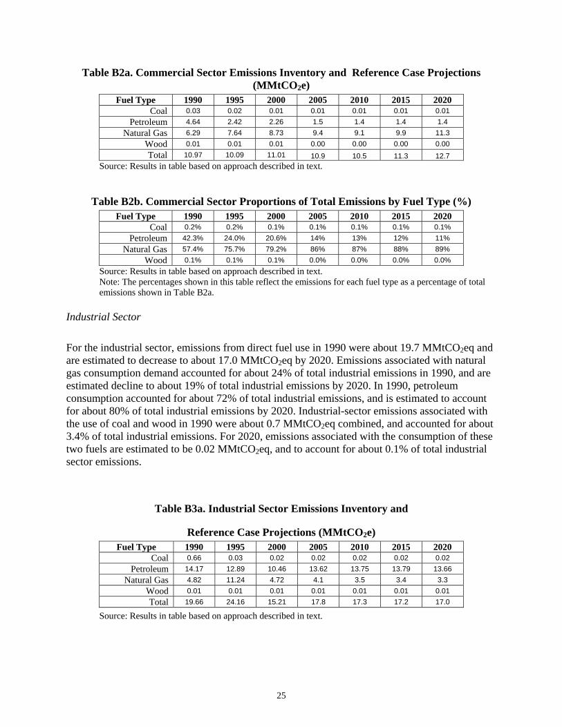
25

Table B2a. Commercial Sector Emissions Inventory and Reference Case Projections (MMtCO2e)

Fuel Type 1990 1995 2000 2005 2010 2015 2020 Coal 0.03 0.02 0.01 0.01 0.01 0.01 0.01

Petroleum 4.64 2.42 2.26 1.5 1.4 1.4 1.4 Natural Gas 6.29 7.64 8.73 9.4 9.1 9.9 11.3

Wood 0.01 0.01 0.01 0.00 0.00 0.00 0.00 Total 10.97 10.09 11.01 10.9 10.5 11.3 12.7

Source: Results in table based on approach described in text.

Table B2b. Commercial Sector Proportions of Total Emissions by Fuel Type (%) Fuel Type 1990 1995 2000 2005 2010 2015 2020

Coal 0.2% 0.2% 0.1% 0.1% 0.1% 0.1% 0.1% Petroleum 42.3% 24.0% 20.6% 14% 13% 12% 11%

Natural Gas 57.4% 75.7% 79.2% 86% 87% 88% 89% Wood 0.1% 0.1% 0.1% 0.0% 0.0% 0.0% 0.0%

Source: Results in table based on approach described in text. Note: The percentages shown in this table reflect the emissions for each fuel type as a percentage of total emissions shown in Table B2a.

Industrial Sector

For the industrial sector, emissions from direct fuel use in 1990 were about 19.7 MMtCO2eq and are estimated to decrease to about 17.0 MMtCO2eq by 2020. Emissions associated with natural gas consumption demand accounted for about 24% of total industrial emissions in 1990, and are estimated decline to about 19% of total industrial emissions by 2020. In 1990, petroleum consumption accounted for about 72% of total industrial emissions, and is estimated to account for about 80% of total industrial emissions by 2020. Industrial-sector emissions associated with the use of coal and wood in 1990 were about 0.7 MMtCO2eq combined, and accounted for about 3.4% of total industrial emissions. For 2020, emissions associated with the consumption of these two fuels are estimated to be 0.02 MMtCO2eq, and to account for about 0.1% of total industrial sector emissions.

Table B3a. Industrial Sector Emissions Inventory and

Reference Case Projections (MMtCO2e) Fuel Type 1990 1995 2000 2005 2010 2015 2020

Coal 0.66 0.03 0.02 0.02 0.02 0.02 0.02 Petroleum 14.17 12.89 10.46 13.62 13.75 13.79 13.66

Natural Gas 4.82 11.24 4.72 4.1 3.5 3.4 3.3 Wood 0.01 0.01 0.01 0.01 0.01 0.01 0.01 Total 19.66 24.16 15.21 17.8 17.3 17.2 17.0

Source: Results in table based on approach described in text.

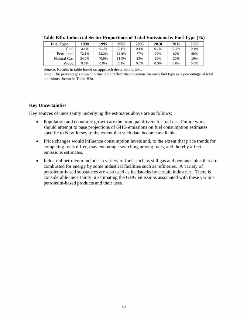
26

Table B3b. Industrial Sector Proportions of Total Emissions by Fuel Type (%)

Fuel Type 1990 1995 2000 2005 2010 2015 2020 Coal 3.4% 0.1% 0.1% 0.1% 0.1% 0.1% 0.1%

Petroleum 72.1% 53.3% 68.8% 77% 79% 80% 80% Natural Gas 24.5% 46.5% 31.0% 23% 20% 20% 19%

Wood 0.0% 0.0% 0.1% 0.0% 0.0% 0.0% 0.0%

Source: Results in table based on approach described in text. Note: The percentages shown in this table reflect the emissions for each fuel type as a percentage of total emissions shown in Table B3a.

Key Uncertainties Key sources of uncertainty underlying the estimates above are as follows:

• Population and economic growth are the principal drivers for fuel use. Future work should attempt to base projections of GHG emissions on fuel consumption estimates specific to New Jersey to the extent that such data become available.

• Price changes would influence consumption levels and, to the extent that price trends for competing fuels differ, may encourage switching among fuels, and thereby affect emissions estimates.

• Industrial petroleum includes a variety of fuels such as still gas and pentanes plus that are combusted for energy by some industrial facilities such as refineries. A variety of petroleum-based substances are also used as feedstocks by certain industries. There is considerable uncertainty in estimating the GHG emissions associated with these various petroleum-based products and their uses.

27

Appendix C. Transportation Energy Use Overview Transportation is the largest greenhouse gas (GHG) source sector in New Jersey –accounting for over one third of New Jersey’s current gross GHG emissions. The transportation sector includes light- and heavy-duty on-road vehicles, aircraft, locomotives, and marine engines. Carbon dioxide (CO2) accounts for about 97% of the transportation sector’s GHG emissions in 1990 and is projected to increase to about 98% of transportation GHG emissions by 2020. Most of the remaining GHG emissions from the transportation sector are due to nitrous oxide (N2O) emissions from gasoline engines. The following discusses the data sources, methods, assumptions, and results used to construct the inventory (1990 to most recent year for which activity data are available (i.e., 2003, 2004, or 2005)), and reference case projections (2004, 2005, or 2006 to 2020) based on business-as-usual assumptions.

Historical Emissions and Reference Case Projections (Business-as-Usual) Historical greenhouse gas emissions were estimated using the United States Environmental Protection Agency’s (US EPA) State Greenhouse Gas Inventory Tool (SGIT) software and the methods provided in the Emission Inventory Improvement Program (EIIP) guidance document for the sector.49,50 In some cases, the SGIT default data or methodologies were refined to account for data or issues specific to New Jersey. Emissions were calculated from 1990 through the most recent year for which the historical activity data were available. This varied from 2003 to 2005, depending upon the data source. For all transportation sectors, the CO2 emission factors are in units of pounds (lb) per million British thermal unit (MMBtu). The methane (CH4) and N2O emission factors are both in units of grams per vehicle mile traveled (VMT) for on-road vehicles and in grams per kilogram of fuel for the aviation, marine vessel, and rail sectors. Key assumptions in this analysis are listed in Table C1. The default fuel consumption data within SGIT were used in most cases to estimate emissions, with the most recently available fuel consumption data (2004) from the United States Department of Energy (US DOE) Energy Information Administration’s (EIA) State Energy Data (SED) added.51

49 CO2 emissions were calculated using SGIT, with reference to Emission Inventory Improvement Program, Volume VIII: Chapter. 1. “Methods for Estimating Carbon Dioxide Emissions from Combustion of Fossil Fuels”, August 2004. 50 CH4 and N2O emissions were calculated using SGIT, with reference to Emission Inventory Improvement Program, Volume VIII: Chapter. 3. “Methods for Estimating Methane and Nitrous Oxide Emissions from Mobile Combustion”, August 2004. 51 Energy Information Administration, State Energy Consumption, Price, and Expenditure Estimates (SED), http://www.eia.doe.gov/emeu/states/_seds.html

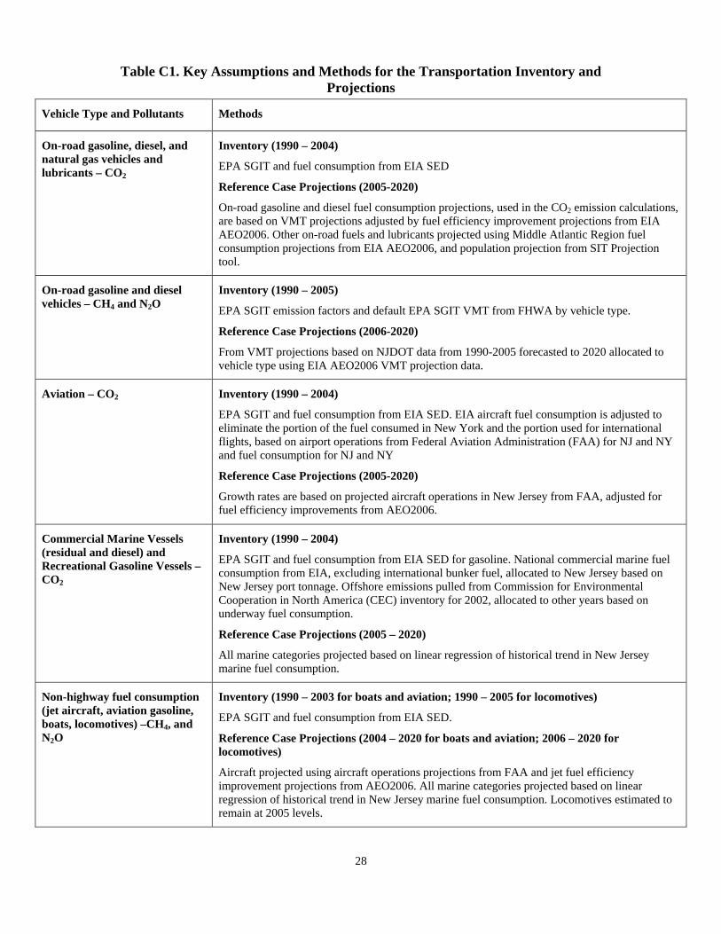
28

Table C1. Key Assumptions and Methods for the Transportation Inventory and Projections

Vehicle Type and Pollutants Methods

On-road gasoline, diesel, and natural gas vehicles and lubricants – CO2

Inventory (1990 – 2004)

EPA SGIT and fuel consumption from EIA SED

Reference Case Projections (2005-2020)

On-road gasoline and diesel fuel consumption projections, used in the CO2 emission calculations, are based on VMT projections adjusted by fuel efficiency improvement projections from EIA AEO2006. Other on-road fuels and lubricants projected using Middle Atlantic Region fuel consumption projections from EIA AEO2006, and population projection from SIT Projection tool.

On-road gasoline and diesel vehicles – CH4 and N2O

Inventory (1990 – 2005)

EPA SGIT emission factors and default EPA SGIT VMT from FHWA by vehicle type.

Reference Case Projections (2006-2020)

From VMT projections based on NJDOT data from 1990-2005 forecasted to 2020 allocated to vehicle type using EIA AEO2006 VMT projection data.

Aviation – CO2 Inventory (1990 – 2004)

EPA SGIT and fuel consumption from EIA SED. EIA aircraft fuel consumption is adjusted to eliminate the portion of the fuel consumed in New York and the portion used for international flights, based on airport operations from Federal Aviation Administration (FAA) for NJ and NY and fuel consumption for NJ and NY

Reference Case Projections (2005-2020)

Growth rates are based on projected aircraft operations in New Jersey from FAA, adjusted for fuel efficiency improvements from AEO2006.

Commercial Marine Vessels (residual and diesel) and Recreational Gasoline Vessels – CO2

Inventory (1990 – 2004)

EPA SGIT and fuel consumption from EIA SED for gasoline. National commercial marine fuel consumption from EIA, excluding international bunker fuel, allocated to New Jersey based on New Jersey port tonnage. Offshore emissions pulled from Commission for Environmental Cooperation in North America (CEC) inventory for 2002, allocated to other years based on underway fuel consumption.

Reference Case Projections (2005 – 2020)

All marine categories projected based on linear regression of historical trend in New Jersey marine fuel consumption.

Non-highway fuel consumption (jet aircraft, aviation gasoline, boats, locomotives) –CH4, and N2O

Inventory (1990 – 2003 for boats and aviation; 1990 – 2005 for locomotives)

EPA SGIT and fuel consumption from EIA SED.

Reference Case Projections (2004 – 2020 for boats and aviation; 2006 – 2020 for locomotives)

Aircraft projected using aircraft operations projections from FAA and jet fuel efficiency improvement projections from AEO2006. All marine categories projected based on linear regression of historical trend in New Jersey marine fuel consumption. Locomotives estimated to remain at 2005 levels.

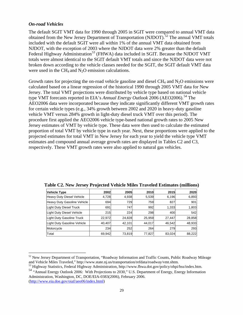
29

On-road Vehicles The default SGIT VMT data for 1990 through 2005 in SGIT were compared to annual VMT data obtained from the New Jersey Department of Transportation (NJDOT).52 The annual VMT totals included with the default SGIT were all within 1% of the annual VMT data obtained from NJDOT, with the exception of 2003 where the NJDOT data were 2% greater than the default Federal Highway Administration53 (FHWA) data included in SGIT. Because the NJDOT VMT totals were almost identical to the SGIT default VMT totals and since the NJDOT data were not broken down according to the vehicle classes needed for the SGIT, the SGIT default VMT data were used in the CH4 and N2O emission calculations. Growth rates for projecting the on-road vehicle gasoline and diesel CH4 and N2O emissions were calculated based on a linear regression of the historical 1990 through 2005 VMT data for New Jersey. The total VMT projections were distributed by vehicle type based on national vehicle type VMT forecasts reported in EIA’s Annual Energy Outlook 2006 (AEO2006).54 The AEO2006 data were incorporated because they indicate significantly different VMT growth rates for certain vehicle types (e.g., 34% growth between 2002 and 2020 in heavy-duty gasoline vehicle VMT versus 284% growth in light-duty diesel truck VMT over this period). The procedure first applied the AEO2006 vehicle type-based national growth rates to 2005 New Jersey estimates of VMT by vehicle type. These data were then used to calculate the estimated proportion of total VMT by vehicle type in each year. Next, these proportions were applied to the projected estimates for total VMT in New Jersey for each year to yield the vehicle type VMT estimates and compound annual average growth rates are displayed in Tables C2 and C3, respectively. These VMT growth rates were also applied to natural gas vehicles.

Table C2. New Jersey Projected Vehicle Miles Traveled Estimates (millions) Vehicle Type 2002 2005 2010 2015 2020Heavy Duty Diesel Vehicle 4,728 4,938 5,539 6,196 6,893Heavy Duty Gasoline Vehicle 694 729 759 827 901Light Duty Diesel Truck 691 747 992 1,333 1,803Light Duty Diesel Vehicle 215 224 298 400 542Light Duty Gasoline Truck 22,972 24,828 25,959 27,447 28,858Light Duty Gasoline Vehicle 40,407 42,101 44,017 46,542 48,933Motorcycle 234 252 264 279 293Total 69,942 73,819 77,827 83,024 88,222

52 New Jersey Department of Transportation, “Roadway Information and Traffic Counts, Public Roadway Mileage and Vehicle Miles Traveled,” http://www.state.nj.us/transportation/refdata/roadway/vmt.shtm. 53 Highway Statistics, Federal Highway Administration, http://www.fhwa.dot.gov/policy/ohpi/hss/index.htm. 54 “Annual Energy Outlook 2006: With Projections to 2030,” U.S. Department of Energy, Energy Information Administration, Washington, DC, DOE/EIA-0383(2006), February 2006. (http://www.eia.doe.gov/oiaf/aeo06/index.html)

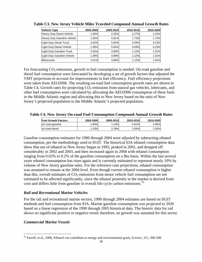
30

Table C3. New Jersey Vehicle Miles Traveled Compound Annual Growth Rates Vehicle Type 2002-2005 2005-2010 2010-2015 2015-2020 Heavy Duty Diesel Vehicle 1.46% 2.32% 2.27% 2.15% Heavy Duty Gasoline Vehicle 1.65% 0.81% 1.73% 1.72% Light Duty Diesel Truck 2.62% 5.84% 6.09% 6.23% Light Duty Diesel Vehicle 1.38% 5.84% 6.09% 6.23% Light Duty Gasoline Truck 2.62% 0.89% 1.12% 1.01% Light Duty Gasoline Vehicle 1.38% 0.89% 1.12% 1.01% Motorcycle 2.51% 0.89% 1.12% 1.01%

For forecasting CO2 emissions, growth in fuel consumption is needed. On-road gasoline and diesel fuel consumption were forecasted by developing a set of growth factors that adjusted the VMT projections to account for improvements in fuel efficiency. Fuel efficiency projections were taken from AEO2006. The resulting on-road fuel consumption growth rates are shown in Table C4. Growth rates for projecting CO2 emissions from natural gas vehicles, lubricants, and other fuel consumption were calculated by allocating the AEO2006 consumption of these fuels in the Middle Atlantic region and allocating this to New Jersey based on the ratio of New Jersey’s projected population to the Middle Atlantic’s projected population.

Table C4. New Jersey On-road Fuel Consumption Compound Annual Growth Rates Fuel Growth Factors 2002-2005 2005-2010 2010-2015 2015-2020 on-road gasoline 1.84% 1.10% 0.61% 0.95% on-road diesel 1.33% 2.29% 2.59% 2.50%

Gasoline consumption estimates for 1990 through 2004 were adjusted by subtracting ethanol consumption, per the methodology used in SGIT. The historical EIA ethanol consumption data show that use of ethanol in New Jersey began in 1993, peaked in 2001, and dropped off considerably in 2002 and 2003, and then increased again in 2004 with ethanol consumption ranging from 0.02% to 0.2% of the gasoline consumption on a Btu basis. Within the last several years ethanol consumption has risen again and is currently estimated to represent nearly 10% by volume of New Jersey gasoline sales. For the reference case projections, ethanol consumption was assumed to remain at the 2004 level. Even though current ethanol consumption is higher than this, overall estimates of CO2 emissions from motor vehicle fuel consumption are not estimated to be affected significantly, since the ethanol presently in the market is derived from corn and differs little from gasoline in overall life cycle carbon emissions.55 Rail and Recreational Marine Vehicles

For the rail and recreational marine sectors, 1990 through 2004 estimates are based on SGIT methods and fuel consumption from EIA. Marine gasoline consumption was projected to 2020 based on a linear regression of the 1990 through 2005 historical data. The historic data for rail shows no significant positive or negative trend; therefore, no growth was assumed for this sector. Commercial Marine Vessels

55 Farrell, et al., 2006, Ethanol can contribute to energy and environmental goals, Science, 311, 506-508.

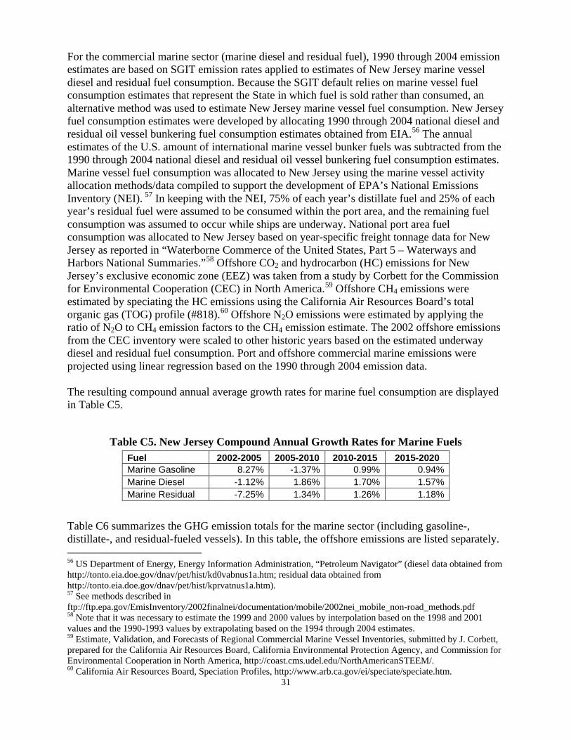
31

For the commercial marine sector (marine diesel and residual fuel), 1990 through 2004 emission estimates are based on SGIT emission rates applied to estimates of New Jersey marine vessel diesel and residual fuel consumption. Because the SGIT default relies on marine vessel fuel consumption estimates that represent the State in which fuel is sold rather than consumed, an alternative method was used to estimate New Jersey marine vessel fuel consumption. New Jersey fuel consumption estimates were developed by allocating 1990 through 2004 national diesel and residual oil vessel bunkering fuel consumption estimates obtained from EIA.56 The annual estimates of the U.S. amount of international marine vessel bunker fuels was subtracted from the 1990 through 2004 national diesel and residual oil vessel bunkering fuel consumption estimates. Marine vessel fuel consumption was allocated to New Jersey using the marine vessel activity allocation methods/data compiled to support the development of EPA’s National Emissions Inventory (NEI). 57 In keeping with the NEI, 75% of each year’s distillate fuel and 25% of each year’s residual fuel were assumed to be consumed within the port area, and the remaining fuel consumption was assumed to occur while ships are underway. National port area fuel consumption was allocated to New Jersey based on year-specific freight tonnage data for New Jersey as reported in “Waterborne Commerce of the United States, Part 5 – Waterways and Harbors National Summaries.”58 Offshore CO2 and hydrocarbon (HC) emissions for New Jersey’s exclusive economic zone (EEZ) was taken from a study by Corbett for the Commission for Environmental Cooperation (CEC) in North America.59 Offshore CH4 emissions were estimated by speciating the HC emissions using the California Air Resources Board’s total organic gas (TOG) profile (#818).60 Offshore N2O emissions were estimated by applying the ratio of N2O to CH4 emission factors to the CH4 emission estimate. The 2002 offshore emissions from the CEC inventory were scaled to other historic years based on the estimated underway diesel and residual fuel consumption. Port and offshore commercial marine emissions were projected using linear regression based on the 1990 through 2004 emission data. The resulting compound annual average growth rates for marine fuel consumption are displayed in Table C5.

Table C5. New Jersey Compound Annual Growth Rates for Marine Fuels Fuel 2002-2005 2005-2010 2010-2015 2015-2020 Marine Gasoline 8.27% -1.37% 0.99% 0.94% Marine Diesel -1.12% 1.86% 1.70% 1.57% Marine Residual -7.25% 1.34% 1.26% 1.18%

Table C6 summarizes the GHG emission totals for the marine sector (including gasoline-, distillate-, and residual-fueled vessels). In this table, the offshore emissions are listed separately. 56 US Department of Energy, Energy Information Administration, “Petroleum Navigator” (diesel data obtained from http://tonto.eia.doe.gov/dnav/pet/hist/kd0vabnus1a.htm; residual data obtained from http://tonto.eia.doe.gov/dnav/pet/hist/kprvatnus1a.htm). 57 See methods described in ftp://ftp.epa.gov/EmisInventory/2002finalnei/documentation/mobile/2002nei_mobile_non-road_methods.pdf 58 Note that it was necessary to estimate the 1999 and 2000 values by interpolation based on the 1998 and 2001 values and the 1990-1993 values by extrapolating based on the 1994 through 2004 estimates. 59 Estimate, Validation, and Forecasts of Regional Commercial Marine Vessel Inventories, submitted by J. Corbett, prepared for the California Air Resources Board, California Environmental Protection Agency, and Commission for Environmental Cooperation in North America, http://coast.cms.udel.edu/NorthAmericanSTEEM/. 60 California Air Resources Board, Speciation Profiles, http://www.arb.ca.gov/ei/speciate/speciate.htm.

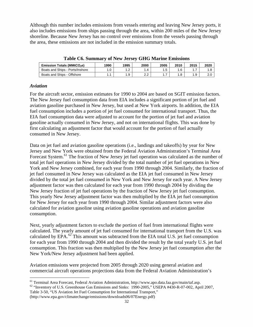
32

Although this number includes emissions from vessels entering and leaving New Jersey ports, it also includes emissions from ships passing through the area, within 200 miles of the New Jersey shoreline. Because New Jersey has no control over emissions from the vessels passing through the area, these emissions are not included in the emission summary totals.

Table C6. Summary of New Jersey GHG Marine Emissions Emission Totals (MMtCO2e) 1990 1995 2000 2005 2010 2015 2020 Boats and Ships - Ports/Inshore 1.0 1.2 1.4 1.5 1.6 1.7 1.8 Boats and Ships - Offshore 1.1 1.9 2.2 1.7 1.8 1.9 2.0

Aviation For the aircraft sector, emission estimates for 1990 to 2004 are based on SGIT emission factors. The New Jersey fuel consumption data from EIA includes a significant portion of jet fuel and aviation gasoline purchased in New Jersey, but used at New York airports. In addition, the EIA fuel consumption includes a portion of jet fuel consumed for international transport. Thus, the EIA fuel consumption data were adjusted to account for the portion of jet fuel and aviation gasoline actually consumed in New Jersey, and not on international flights. This was done by first calculating an adjustment factor that would account for the portion of fuel actually consumed in New Jersey. Data on jet fuel and aviation gasoline operations (i.e., landings and takeoffs) by year for New Jersey and New York were obtained from the Federal Aviation Administration’s Terminal Area Forecast System.61 The fraction of New Jersey jet fuel operation was calculated as the number of total jet fuel operations in New Jersey divided by the total number of jet fuel operations in New York and New Jersey combined, for each year from 1990 through 2004. Similarly, the fraction of jet fuel consumed in New Jersey was calculated as the EIA jet fuel consumed in New Jersey divided by the total jet fuel consumed in New York and New Jersey for each year. A New Jersey adjustment factor was then calculated for each year from 1990 through 2004 by dividing the New Jersey fraction of jet fuel operations by the fraction of New Jersey jet fuel consumption. This yearly New Jersey adjustment factor was then multiplied by the EIA jet fuel consumption for New Jersey for each year from 1990 through 2004. Similar adjustment factors were also calculated for aviation gasoline using aviation gasoline operations and aviation gasoline consumption. Next, yearly adjustment factors to exclude the portion of fuel from international flights were calculated. The yearly amount of jet fuel consumed for international transport from the U.S. was calculated by EPA.62 This amount was subtracted from the EIA total U.S. jet fuel consumption for each year from 1990 through 2004 and then divided the result by the total yearly U.S. jet fuel consumption. This fraction was then multiplied by the New Jersey jet fuel consumption after the New York/New Jersey adjustment had been applied. Aviation emissions were projected from 2005 through 2020 using general aviation and commercial aircraft operations projections data from the Federal Aviation Administration’s 61 Terminal Area Forecast, Federal Aviation Administration, http://www.apo.data.faa.gov/main/taf.asp. 62 “Inventory of U.S. Greenhouse Gas Emissions and Sinks: 1990-2005,” USEPA #430-R-07-002, April 2007, Table 3-50, “US Aviation Jet Fuel Consumption for International Transport,” (http://www.epa.gov/climatechange/emissions/downloads06/07Energy.pdf)

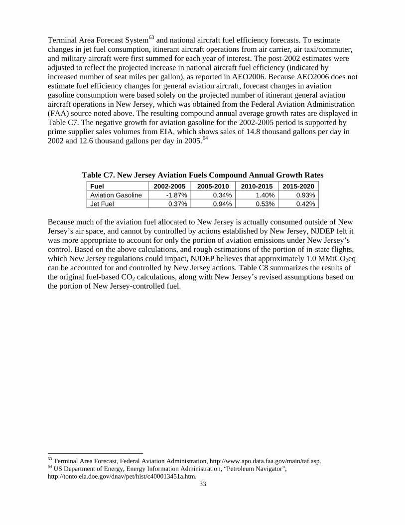
33

Terminal Area Forecast System63 and national aircraft fuel efficiency forecasts. To estimate changes in jet fuel consumption, itinerant aircraft operations from air carrier, air taxi/commuter, and military aircraft were first summed for each year of interest. The post-2002 estimates were adjusted to reflect the projected increase in national aircraft fuel efficiency (indicated by increased number of seat miles per gallon), as reported in AEO2006. Because AEO2006 does not estimate fuel efficiency changes for general aviation aircraft, forecast changes in aviation gasoline consumption were based solely on the projected number of itinerant general aviation aircraft operations in New Jersey, which was obtained from the Federal Aviation Administration (FAA) source noted above. The resulting compound annual average growth rates are displayed in Table C7. The negative growth for aviation gasoline for the 2002-2005 period is supported by prime supplier sales volumes from EIA, which shows sales of 14.8 thousand gallons per day in 2002 and 12.6 thousand gallons per day in 2005.64

Table C7. New Jersey Aviation Fuels Compound Annual Growth Rates Fuel 2002-2005 2005-2010 2010-2015 2015-2020 Aviation Gasoline -1.87% 0.34% 1.40% 0.93% Jet Fuel 0.37% 0.94% 0.53% 0.42%

Because much of the aviation fuel allocated to New Jersey is actually consumed outside of New Jersey’s air space, and cannot by controlled by actions established by New Jersey, NJDEP felt it was more appropriate to account for only the portion of aviation emissions under New Jersey’s control. Based on the above calculations, and rough estimations of the portion of in-state flights, which New Jersey regulations could impact, NJDEP believes that approximately 1.0 MMtCO2eq can be accounted for and controlled by New Jersey actions. Table C8 summarizes the results of the original fuel-based CO2 calculations, along with New Jersey’s revised assumptions based on the portion of New Jersey-controlled fuel.

63 Terminal Area Forecast, Federal Aviation Administration, http://www.apo.data.faa.gov/main/taf.asp. 64 US Department of Energy, Energy Information Administration, “Petroleum Navigator”, http://tonto.eia.doe.gov/dnav/pet/hist/c400013451a.htm.

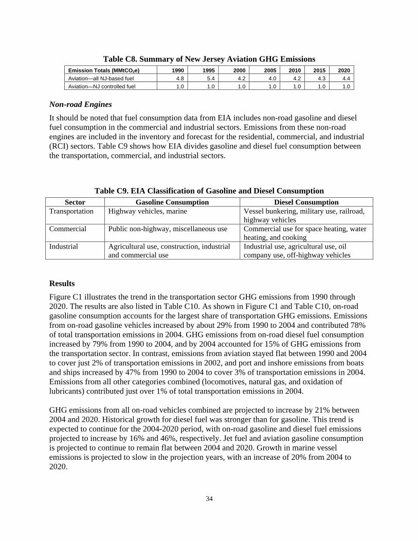
34

Table C8. Summary of New Jersey Aviation GHG Emissions Emission Totals (MMtCO2e) 1990 1995 2000 2005 2010 2015 2020 Aviation—all NJ-based fuel 4.8 5.4 4.2 4.0 4.2 4.3 4.4 Aviation—NJ controlled fuel 1.0 1.0 1.0 1.0 1.0 1.0 1.0

Non-road Engines It should be noted that fuel consumption data from EIA includes non-road gasoline and diesel fuel consumption in the commercial and industrial sectors. Emissions from these non-road engines are included in the inventory and forecast for the residential, commercial, and industrial (RCI) sectors. Table C9 shows how EIA divides gasoline and diesel fuel consumption between the transportation, commercial, and industrial sectors.

Table C9. EIA Classification of Gasoline and Diesel Consumption Sector Gasoline Consumption Diesel Consumption

Transportation Highway vehicles, marine Vessel bunkering, military use, railroad, highway vehicles

Commercial Public non-highway, miscellaneous use Commercial use for space heating, water heating, and cooking

Industrial Agricultural use, construction, industrial and commercial use

Industrial use, agricultural use, oil company use, off-highway vehicles

Results Figure C1 illustrates the trend in the transportation sector GHG emissions from 1990 through 2020. The results are also listed in Table C10. As shown in Figure C1 and Table C10, on-road gasoline consumption accounts for the largest share of transportation GHG emissions. Emissions from on-road gasoline vehicles increased by about 29% from 1990 to 2004 and contributed 78% of total transportation emissions in 2004. GHG emissions from on-road diesel fuel consumption increased by 79% from 1990 to 2004, and by 2004 accounted for 15% of GHG emissions from the transportation sector. In contrast, emissions from aviation stayed flat between 1990 and 2004 to cover just 2% of transportation emissions in 2002, and port and inshore emissions from boats and ships increased by 47% from 1990 to 2004 to cover 3% of transportation emissions in 2004. Emissions from all other categories combined (locomotives, natural gas, and oxidation of lubricants) contributed just over 1% of total transportation emissions in 2004. GHG emissions from all on-road vehicles combined are projected to increase by 21% between 2004 and 2020. Historical growth for diesel fuel was stronger than for gasoline. This trend is expected to continue for the 2004-2020 period, with on-road gasoline and diesel fuel emissions projected to increase by 16% and 46%, respectively. Jet fuel and aviation gasoline consumption is projected to continue to remain flat between 2004 and 2020. Growth in marine vessel emissions is projected to slow in the projection years, with an increase of 20% from 2004 to 2020.

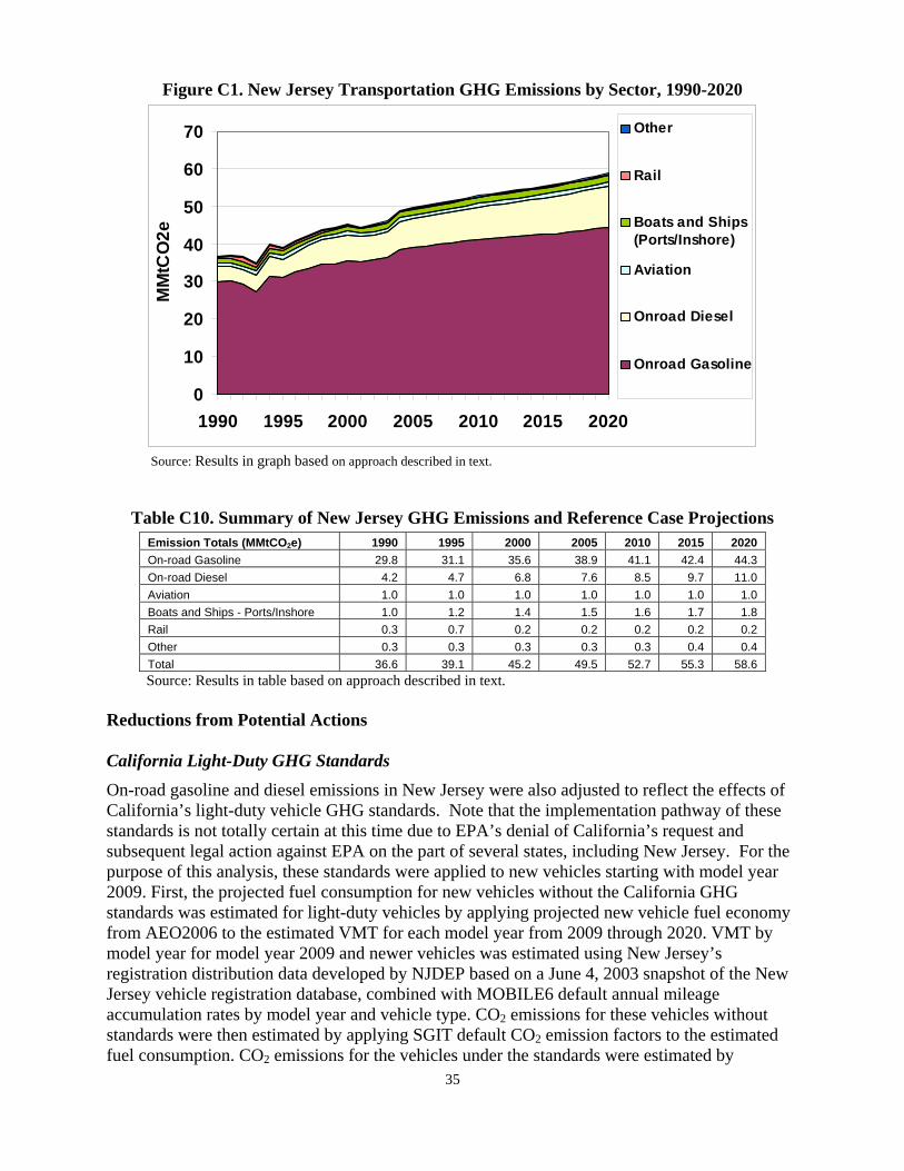
35

Figure C1. New Jersey Transportation GHG Emissions by Sector, 1990-2020

0

10

20

30

40

50

60

70

1990 1995 2000 2005 2010 2015 2020

MM

tCO

2e

Other

Rail

Boats and Ships(Ports/Inshore)

Aviation

Onroad Diesel

Onroad Gasoline

Source: Results in graph based on approach described in text.

Table C10. Summary of New Jersey GHG Emissions and Reference Case Projections Emission Totals (MMtCO2e) 1990 1995 2000 2005 2010 2015 2020 On-road Gasoline 29.8 31.1 35.6 38.9 41.1 42.4 44.3 On-road Diesel 4.2 4.7 6.8 7.6 8.5 9.7 11.0 Aviation 1.0 1.0 1.0 1.0 1.0 1.0 1.0 Boats and Ships - Ports/Inshore 1.0 1.2 1.4 1.5 1.6 1.7 1.8 Rail 0.3 0.7 0.2 0.2 0.2 0.2 0.2 Other 0.3 0.3 0.3 0.3 0.3 0.4 0.4 Total 36.6 39.1 45.2 49.5 52.7 55.3 58.6 Source: Results in table based on approach described in text.

Reductions from Potential Actions California Light-Duty GHG Standards

On-road gasoline and diesel emissions in New Jersey were also adjusted to reflect the effects of California’s light-duty vehicle GHG standards. Note that the implementation pathway of these standards is not totally certain at this time due to EPA’s denial of California’s request and subsequent legal action against EPA on the part of several states, including New Jersey. For the purpose of this analysis, these standards were applied to new vehicles starting with model year 2009. First, the projected fuel consumption for new vehicles without the California GHG standards was estimated for light-duty vehicles by applying projected new vehicle fuel economy from AEO2006 to the estimated VMT for each model year from 2009 through 2020. VMT by model year for model year 2009 and newer vehicles was estimated using New Jersey’s registration distribution data developed by NJDEP based on a June 4, 2003 snapshot of the New Jersey vehicle registration database, combined with MOBILE6 default annual mileage accumulation rates by model year and vehicle type. CO2 emissions for these vehicles without standards were then estimated by applying SGIT default CO2 emission factors to the estimated fuel consumption. CO2 emissions for the vehicles under the standards were estimated by

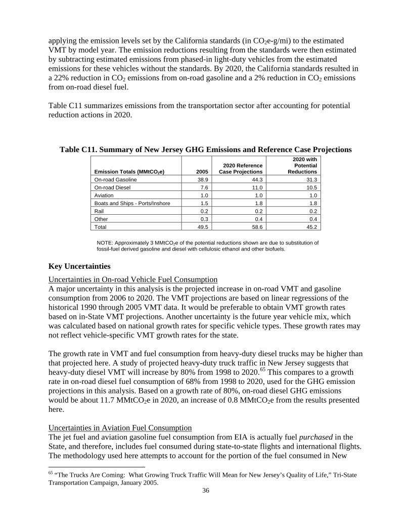
36

applying the emission levels set by the California standards (in CO2e-g/mi) to the estimated VMT by model year. The emission reductions resulting from the standards were then estimated by subtracting estimated emissions from phased-in light-duty vehicles from the estimated emissions for these vehicles without the standards. By 2020, the California standards resulted in a 22% reduction in CO2 emissions from on-road gasoline and a 2% reduction in CO2 emissions from on-road diesel fuel. Table C11 summarizes emissions from the transportation sector after accounting for potential reduction actions in 2020.

Table C11. Summary of New Jersey GHG Emissions and Reference Case Projections

Emission Totals (MMtCO2e) 2005 2020 Reference

Case Projections

2020 with Potential

Reductions On-road Gasoline 38.9 44.3 31.3 On-road Diesel 7.6 11.0 10.5 Aviation 1.0 1.0 1.0 Boats and Ships - Ports/Inshore 1.5 1.8 1.8 Rail 0.2 0.2 0.2 Other 0.3 0.4 0.4 Total 49.5 58.6 45.2

NOTE: Approximately 3 MMtCO2e of the potential reductions shown are due to substitution of fossil-fuel derived gasoline and diesel with cellulosic ethanol and other biofuels. Key Uncertainties Uncertainties in On-road Vehicle Fuel Consumption A major uncertainty in this analysis is the projected increase in on-road VMT and gasoline consumption from 2006 to 2020. The VMT projections are based on linear regressions of the historical 1990 through 2005 VMT data. It would be preferable to obtain VMT growth rates based on in-State VMT projections. Another uncertainty is the future year vehicle mix, which was calculated based on national growth rates for specific vehicle types. These growth rates may not reflect vehicle-specific VMT growth rates for the state. The growth rate in VMT and fuel consumption from heavy-duty diesel trucks may be higher than that projected here. A study of projected heavy-duty truck traffic in New Jersey suggests that heavy-duty diesel VMT will increase by 80% from 1998 to 2020.65 This compares to a growth rate in on-road diesel fuel consumption of 68% from 1998 to 2020, used for the GHG emission projections in this analysis. Based on a growth rate of 80%, on-road diesel GHG emissions would be about 11.7 MMtCO2e in 2020, an increase of 0.8 MMtCO2e from the results presented here.

Uncertainties in Aviation Fuel Consumption The jet fuel and aviation gasoline fuel consumption from EIA is actually fuel purchased in the State, and therefore, includes fuel consumed during state-to-state flights and international flights. The methodology used here attempts to account for the portion of the fuel consumed in New 65 “The Trucks Are Coming: What Growing Truck Traffic Will Mean for New Jersey’s Quality of Life,” Tri-State Transportation Campaign, January 2005.

37

York and the portion consumed in international flights. However, the methodology used to estimate the portion of fuel consumed on international flights assumes that each State’s share of international aviation fuel consumption is the same as the State’s share of total aviation jet fuel consumption. It is likely that New Jersey’s share of fuel consumption for international flights would be higher than this, indicating that aviation emissions for New Jersey may be overestimated. Uncertainties in Marine Fuel Consumption There are several assumptions that introduce uncertainty into the estimates of commercial marine fuel consumption. These assumptions include:

• 75% of marine diesel and 25% of residual fuel is consumed in port;

• The proportion of freight tonnage for New Jersey as a fraction of national freight tonnage appropriately represents marine fuel that is consumed in New Jersey;

• The 2002 estimate of underway emissions for New Jersey includes marine vessel travel 200 miles out to sea. This may actually include marine vessels traveling to New York ports, as well as New Jersey ports, which may lead to an overestimation of the underway marine vessel emissions.

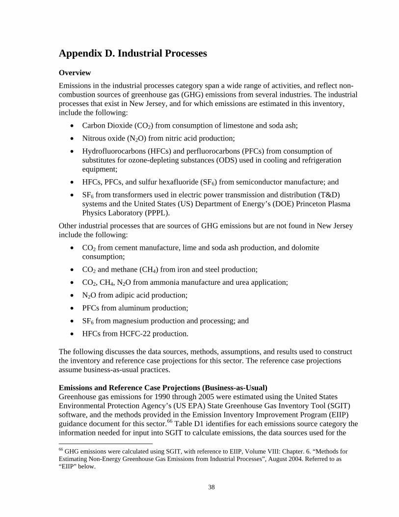
38

Appendix D. Industrial Processes Overview Emissions in the industrial processes category span a wide range of activities, and reflect non-combustion sources of greenhouse gas (GHG) emissions from several industries. The industrial processes that exist in New Jersey, and for which emissions are estimated in this inventory, include the following:

• Carbon Dioxide (CO2) from consumption of limestone and soda ash; • Nitrous oxide (N2O) from nitric acid production; • Hydrofluorocarbons (HFCs) and perfluorocarbons (PFCs) from consumption of

substitutes for ozone-depleting substances (ODS) used in cooling and refrigeration equipment;

• HFCs, PFCs, and sulfur hexafluoride (SF6) from semiconductor manufacture; and • SF6 from transformers used in electric power transmission and distribution (T&D)

systems and the United States (US) Department of Energy’s (DOE) Princeton Plasma Physics Laboratory (PPPL).

Other industrial processes that are sources of GHG emissions but are not found in New Jersey include the following:

• CO2 from cement manufacture, lime and soda ash production, and dolomite consumption;

• CO2 and methane (CH4) from iron and steel production; • CO2, CH4, N2O from ammonia manufacture and urea application; • N2O from adipic acid production; • PFCs from aluminum production; • SF6 from magnesium production and processing; and • HFCs from HCFC-22 production.

The following discusses the data sources, methods, assumptions, and results used to construct the inventory and reference case projections for this sector. The reference case projections assume business-as-usual practices. Emissions and Reference Case Projections (Business-as-Usual) Greenhouse gas emissions for 1990 through 2005 were estimated using the United States Environmental Protection Agency’s (US EPA) State Greenhouse Gas Inventory Tool (SGIT) software, and the methods provided in the Emission Inventory Improvement Program (EIIP) guidance document for this sector.66 Table D1 identifies for each emissions source category the information needed for input into SGIT to calculate emissions, the data sources used for the 66 GHG emissions were calculated using SGIT, with reference to EIIP, Volume VIII: Chapter. 6. “Methods for Estimating Non-Energy Greenhouse Gas Emissions from Industrial Processes”, August 2004. Referred to as “EIIP” below.

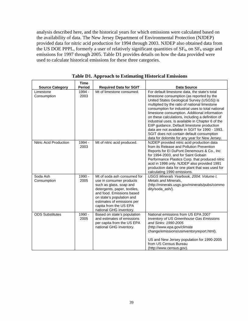
39

analysis described here, and the historical years for which emissions were calculated based on the availability of data. The New Jersey Department of Environmental Protection (NJDEP) provided data for nitric acid production for 1994 through 2003. NJDEP also obtained data from the US DOE PPPL, formerly a user of relatively significant quantities of SF6, on SF6 usage and emissions for 1997 through 2005. Table D1 provides details on how the data provided were used to calculate historical emissions for these three categories.

Table D1. Approach to Estimating Historical Emissions

Source Category Time

Period Required Data for SGIT Data Source Limestone Consumption

1994 - 2003

Mt of limestone consumed. For default limestone data, the state's total limestone consumption (as reported by the United States Geological Survey (USGS)) is multiplied by the ratio of national limestone consumption for industrial uses to total national limestone consumption. Additional information on these calculations, including a definition of industrial uses, is available in Chapter 6 of the EIIP guidance. Default limestone production data are not available in SGIT for 1990 - 1993. SGIT does not contain default consumption data for dolomite for any year for New Jersey.

Nitric Acid Production 1994 - 2003

Mt of nitric acid produced. NJDEP provided nitric acid production data from its Release and Pollution Prevention Reports for EI DuPont Denemours & Co., Inc for 1994-2003, and for Saint Gobain Performance Plastics Corp. that produced nitric acid in 1998 only. NJDEP also provided 1991 production data for one plant that was used for calculating 1990 emissions.

Soda Ash Consumption

1990 - 2005

Mt of soda ash consumed for use in consumer products such as glass, soap and detergents, paper, textiles, and food. Emissions based on state’s population and estimates of emissions per capita from the US EPA national GHG inventory.

USGS Minerals Yearbook, 2004: Volume I, Metals and Minerals, (http://minerals.usgs.gov/minerals/pubs/commodity/soda_ash/).

ODS Substitutes 1990 - 2005

Based on state’s population and estimates of emissions per capita from the US EPA national GHG inventory.

National emissions from US EPA 2007 Inventory of US Greenhouse Gas Emissions and Sinks: 1990-2005 (http://www.epa.gov/climate change/emissions/usinventoryreport.html). US and New Jersey population for 1990-2005 from US Census Bureau (http://www.census.gov).

40

Table D1. Approach to Estimating Historical Emissions (Continued)

Source Category Time

Period Required Data for SGIT Data Source Semiconductor Manufacturing

1990 - 2005

State and national value of semiconductor shipments for NAICS code 334413 (Semiconductor and Related Device Manufacturing). Method uses ratio of state-to-national value of semiconductor shipments to estimate state’s proportion of national emissions for 1990 - 2005.

National emissions from US EPA 2007 Inventory of US Greenhouse Gas Emissions and Sinks: 1990-2005 (http://www.epa.gov/climate change/emissions/usinventoryreport.html). Value of shipments from U.S Census Bureau's 1997 and 2002 Economic Census (http://www.census.gov/econ/ census02/). For 1997, value of shipments for state was 0.6% of national total. For 2002, value of shipments for

Electric Power T&D Systems

1990 - 2005

Emissions from 1990 to 2005 based on the national emissions per kWh and state's electricity use provided in SGIT.

National emissions per kWh from US EPA 2007 “Inventory of US Greenhouse Gas Emissions and Sinks: 1990-2005” (http://www.epa.gov/climatechange/emissions/usinventoryreport.html).

Laboratory Use of SF6 1990 - 2005

Mt of SF6 gas released to atmosphere.

PPPL provided estimates of SF6 annual leak rates for 1997-2005.

Table D2 lists the data sources used to quantify activities related to industrial process emissions, the annual compound growth rates implied by estimates of future activity used, and the years for which the reference case projections were calculated.

Table D2. Approach to Estimating Projections Annual Growth Rates (%)

Time

Period Projection

Assumptions Data Source

2000 to

2005

2005 to

2010

2010 to

2015

2015 to

2020 Limestone Consumption

2004 - 2020

Compound annual employment growth rate for New Jersey’s manufacturing sector for 2000-2010. Assumed no change in activity from 2004-2005.

Based on R/ECON modeling forecast of manufacturing employment for 2006-2020.a

0.0% -1.3% -1.0% -0.4%

Nitric Acid Production

2004 - 2020

Ditto Ditto 0.0% -1.3% -1.0% -0.4%

Soda Ash Consumption

2006 - 2020

Growth between 2004 and 2009 is projected to be about 0.5% per year for US production. Assumed growth is same for 2010 – 2020.

Minerals Yearbook, 2005: Volume I, Soda Ash, (http://minerals.usgs.gov/minerals/pubs/commodity/soda_ash/soda_myb05.pdf).

0.5 0.5 0.5 0.5

a CEEEP, 2007, Center for Energy, Economic & Environmental Policy (CEEEP), Edward J. Bloustein School of Planning and Public Policy, Rutgers, The State University of New Jersey, 33 Livingston Ave., Room 154, New Brunswick, NJ 08901 (http://www.policy.rutgers.edu/cupr/recon/index.php). Data provided by Nancy Mantell to CCS on March 30, 2007 (file named “Electricity Prelim Data (3-30-07).xls”).

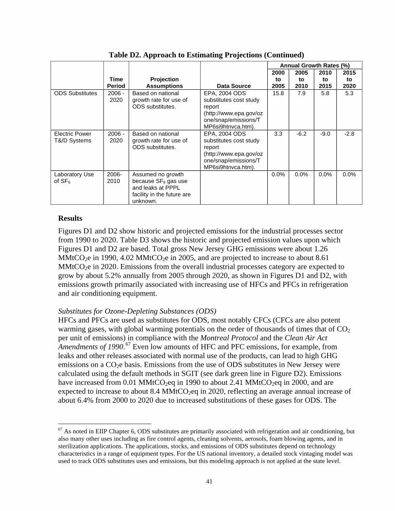
41

Table D2. Approach to Estimating Projections (Continued) Annual Growth Rates (%)

Time

Period Projection

Assumptions Data Source

2000 to

2005

2005 to

2010

2010 to

2015

2015 to

2020 ODS Substitutes 2006 -

2020 Based on national growth rate for use of ODS substitutes.

EPA, 2004 ODS substitutes cost study report (http://www.epa.gov/ozone/snap/emissions/TMP6si9htnvca.htm).

15.8 7.9 5.8 5.3

Electric Power T&/D Systems

2006 - 2020

Based on national growth rate for use of ODS substitutes.

EPA, 2004 ODS substitutes cost study report (http://www.epa.gov/ozone/snap/emissions/TMP6si9htnvca.htm).

3.3 -6.2 -9.0 -2.8

Laboratory Use of SF6

2006-2010

Assumed no growth because SF6 gas use and leaks at PPPL facility in the future are unknown.

0.0% 0.0% 0.0% 0.0%

Results Figures D1 and D2 show historic and projected emissions for the industrial processes sector from 1990 to 2020. Table D3 shows the historic and projected emission values upon which Figures D1 and D2 are based. Total gross New Jersey GHG emissions were about 1.26 MMtCO2e in 1990, 4.02 MMtCO2e in 2005, and are projected to increase to about 8.61 MMtCO2e in 2020. Emissions from the overall industrial processes category are expected to grow by about 5.2% annually from 2005 through 2020, as shown in Figures D1 and D2, with emissions growth primarily associated with increasing use of HFCs and PFCs in refrigeration and air conditioning equipment. Substitutes for Ozone-Depleting Substances (ODS) HFCs and PFCs are used as substitutes for ODS, most notably CFCs (CFCs are also potent warming gases, with global warming potentials on the order of thousands of times that of CO2 per unit of emissions) in compliance with the Montreal Protocol and the Clean Air Act Amendments of 1990.67 Even low amounts of HFC and PFC emissions, for example, from leaks and other releases associated with normal use of the products, can lead to high GHG emissions on a CO2e basis. Emissions from the use of ODS substitutes in New Jersey were calculated using the default methods in SGIT (see dark green line in Figure D2). Emissions have increased from 0.01 MMtCO2eq in 1990 to about 2.41 MMtCO2eq in 2000, and are expected to increase to about 8.4 MMtCO2eq in 2020, reflecting an average annual increase of about 6.4% from 2000 to 2020 due to increased substitutions of these gases for ODS. The

67 As noted in EIIP Chapter 6, ODS substitutes are primarily associated with refrigeration and air conditioning, but also many other uses including as fire control agents, cleaning solvents, aerosols, foam blowing agents, and in sterilization applications. The applications, stocks, and emissions of ODS substitutes depend on technology characteristics in a range of equipment types. For the US national inventory, a detailed stock vintaging model was used to track ODS substitutes uses and emissions, but this modeling approach is not applied at the state level.

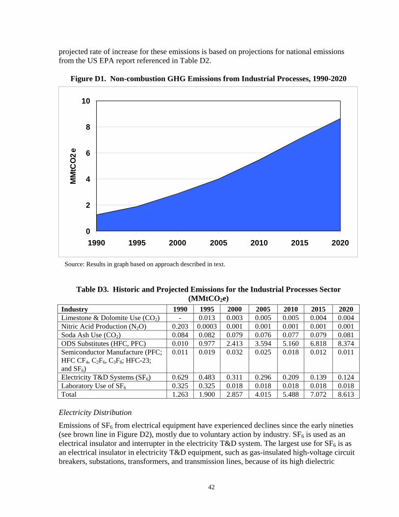
42

projected rate of increase for these emissions is based on projections for national emissions from the US EPA report referenced in Table D2.

Figure D1. Non-combustion GHG Emissions from Industrial Processes, 1990-2020

0

2

4

6

8

10

1990 1995 2000 2005 2010 2015 2020

MM

tCO

2e

Source: Results in graph based on approach described in text.

Table D3. Historic and Projected Emissions for the Industrial Processes Sector (MMtCO2e)

Industry 1990 1995 2000 2005 2010 2015 2020 Limestone & Dolomite Use (CO2) - 0.013 0.003 0.005 0.005 0.004 0.004 Nitric Acid Production (N2O) 0.203 0.0003 0.001 0.001 0.001 0.001 0.001 Soda Ash Use (CO2) 0.084 0.082 0.079 0.076 0.077 0.079 0.081 ODS Substitutes (HFC, PFC) 0.010 0.977 2.413 3.594 5.160 6.818 8.374 Semiconductor Manufacture (PFC; HFC CF4, C2F6, C3F8; HFC-23; and SF6)

0.011 0.019 0.032 0.025 0.018 0.012 0.011

Electricity T&D Systems (SF6) 0.629 0.483 0.311 0.296 0.209 0.139 0.124 Laboratory Use of SF6 0.325 0.325 0.018 0.018 0.018 0.018 0.018 Total 1.263 1.900 2.857 4.015 5.488 7.072 8.613

Electricity Distribution

Emissions of SF6 from electrical equipment have experienced declines since the early nineties (see brown line in Figure D2), mostly due to voluntary action by industry. SF6 is used as an electrical insulator and interrupter in the electricity T&D system. The largest use for SF6 is as an electrical insulator in electricity T&D equipment, such as gas-insulated high-voltage circuit breakers, substations, transformers, and transmission lines, because of its high dielectric

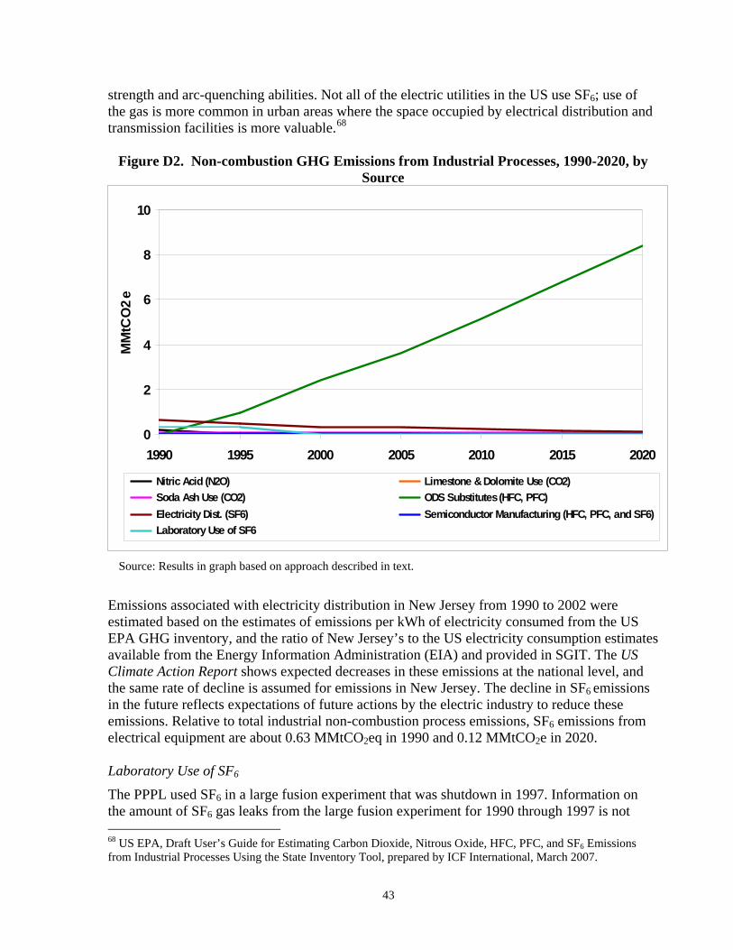
43

strength and arc-quenching abilities. Not all of the electric utilities in the US use SF6; use of the gas is more common in urban areas where the space occupied by electrical distribution and transmission facilities is more valuable.68

Figure D2. Non-combustion GHG Emissions from Industrial Processes, 1990-2020, by

Source

0

2

4

6

8

10

1990 1995 2000 2005 2010 2015 2020

MM

tCO

2e

Nitric Acid (N2O) Limestone & Dolomite Use (CO2) Soda Ash Use (CO2) ODS Substitutes (HFC, PFC) Electricity Dist. (SF6) Semiconductor Manufacturing (HFC, PFC, and SF6) Laboratory Use of SF6

Source: Results in graph based on approach described in text.

Emissions associated with electricity distribution in New Jersey from 1990 to 2002 were estimated based on the estimates of emissions per kWh of electricity consumed from the US EPA GHG inventory, and the ratio of New Jersey’s to the US electricity consumption estimates available from the Energy Information Administration (EIA) and provided in SGIT. The US Climate Action Report shows expected decreases in these emissions at the national level, and the same rate of decline is assumed for emissions in New Jersey. The decline in SF6 emissions in the future reflects expectations of future actions by the electric industry to reduce these emissions. Relative to total industrial non-combustion process emissions, SF6 emissions from electrical equipment are about 0.63 MMtCO2eq in 1990 and 0.12 MMtCO2e in 2020. Laboratory Use of SF6

The PPPL used SF6 in a large fusion experiment that was shutdown in 1997. Information on the amount of SF6 gas leaks from the large fusion experiment for 1990 through 1997 is not 68 US EPA, Draft User’s Guide for Estimating Carbon Dioxide, Nitrous Oxide, HFC, PFC, and SF6 Emissions from Industrial Processes Using the State Inventory Tool, prepared by ICF International, March 2007.

44

available, but was earlier estimated as being in the range of 28,000 to 36,000 pounds per year.69 Since 1997, PPPL has been operating an experiment that requires much less SF6 than the prior experiment. PPPL estimates that it purchases from 2,400 to 4,700 pounds of SF6 annually, and about 1,100 to 2,300 pounds are assumed to leak into the atmosphere annually. Some of the gas is contained in the equipment. During maintenance on equipment that requires removal of the SF6 gas, PPPL uses SF6 reclamation equipment to recover, clean, and reuse as much SF6 gas as possible from the equipment.70 Relative to total industrial non-combustion process emissions, SF6 emissions from PPPL equipment are estimated to average about 0.018 MMtCO2e annually from 1998 through 2005. Based on the range of gas leaks provided by PPPL, emissions may be as low as 0.012 MMtCO2e or as high as 0.025 MMtCO2e annually. For the purpose of this preliminary inventory, emissions for 1990 through 1997 were estimated to be about 0.325 MMtCO2e per year based on an assumption that 30,000 pounds per year of SF6 gas was released to the atmosphere annually. Based on the range of gas leaks provided by PPPL, emissions may be as low as 0.304 MMtCO2e or as high as 0.39 MMtCO2e annually for 1990 through 1997. Because of scaling effects, emissions for this category cannot be seen in Figure D2 after year 2000. Nitric Acid Production

The manufacture of nitric acid (HNO3) produces N2O as a by-product, via the oxidation of ammonia. Nitric acid is a raw material used primarily to make synthetic commercial fertilizer. It is also a major component in the production of adipic acid (a feedstock for nylon) and explosives. Relatively small quantities of nitric acid are also employed for stainless steel pickling, metal etching, rocket propellants, and nuclear fuel processing.71 The NJDEP provided nitric acid production data from its Release and Pollution Prevention Reports. Data were provided for EI DuPont Denemours & Co., Inc for 1994-2003, and for Saint Gobain Performance Plastics Corp. that produced nitric acid in 1998 only. Total production for each year was entered into the SGIT to calculate GHG emissions. The SGIT uses a default emission factor of 0.008 metric tons of N2O emissions per metric ton of nitric acid produced based on a weighted-average calculated over the different types of emissions control technologies typically employed by nitric acid plants nationwide.72

69 NJDEP and NJBPU, 1996, New Jersey Inventory of Greenhouse Gas Emissions, 1990, prepared by Cameron Johnson and Michael Aucott, Division of Science and Research, NJDEP, Trenton, NJ. 70 E-mail from Jerry Levine, PPPL, to Mike Aucott, NJDEP, May 31, 2007. 71 EIIP, Volume VIII: Chapter. 6. “Methods for Estimating Non-Energy Greenhouse Gas Emissions from Industrial Processes”, August 2004. 72 According to Chapter 6 of the EIIP guidance document, the nitric industry controls for oxides of nitrogen through two technologies: non-selective catalytic reduction (NSCR) and SCR. Only one of these technologies, NSCR, is effective at destroying N2O emissions in the process of destroying oxides of nitrogen emissions. NSCR technology was widely installed in nitric acid plants built between 1971 and 1977. Due to high-energy costs and associated high gas temperatures, this technology has not been popular with modern plants. Only about 20% of the current plants have NSCR technology installed. All other plants have installed SCR technology. Since 80% of the current plants have SCR technology installed and 20% have NSCR technology, the weighted-average emission factor used in the SGIT is equal to (0.0095 x 0.80) x (0.002 x 0.20) = 0.008 metric tons N2O per metric ton of nitric acid produced.

45

The NJDEP and BPU prepared a GHG emissions inventory for 1990. The documentation for this inventory provided 1990 production of nitric acid for one plant of 119,070 metric tons (131,250 short tons) and an emission factor of 0.0055 tons of N2O per ton of nitric acid produced.73 This information was used to estimate emissions for 1990, and a GWP of 310 was used to convert emissions to a MMtCO2eq basis. Growth rates for New Jersey’s manufacturing sector for 2006 through 2020 were used to forecast emissions (see Table D2). Emissions for 2004 and 2005 were held constant at 2003 levels (i.e., the last year for which production data were available). Relative to total industrial non-combustion process emissions, estimated emissions associated with nitric acid production are low (about 0.0003 MMtCO2eq in 1995 and 0.001 MMtCO2e in 2020), and therefore, appear at the bottom of Figure D2 due to scaling effects. Semiconductor Manufacture

The semiconductor industry uses fluorinated gases (PFCs [CF4, C2F6, and C3F8]; HFC-23; and SF6) in plasma etching and chemical vapor deposition processes. Emissions of SF6 and HFCs from the manufacture of semiconductors have experienced declines since 2000). Emissions for New Jersey from 1990 to 2002 were estimated based on the default estimates provided in SGIT, which uses the ratio of the state-to-national value of semiconductor shipments to estimate the state’s proportion of national emissions from the US EPA GHG inventory (US EPA 2007 Inventory of US Greenhouse Gas Emissions and Sinks: 1990-2005). The US Climate Action Report shows expected decreases in these emissions at the national level, and the same rate of decline is assumed for emissions in New Jersey. The decline in emissions in the future reflects expectations of future actions by the semiconductor industry to reduce these emissions. Relative to total industrial non-combustion process emissions, emissions associated with the manufacture of semiconductors are low (about 0.011 MMtCO2eq in 1990, 0.025 MMtCO2eq in 2005, and projected to return to 1990 levels of 0.011 MMtCO2eq in 2020), and therefore appear at the bottom of Figure D2 due to scaling effects. Limestone Consumption

Limestone and dolomite are basic raw materials used by a wide variety of industries, including the construction, agriculture, chemical, glass manufacturing, and environmental pollution control industries, as well as in metallurgical industries such as magnesium production.74 Historical state-specific data for New Jersey were not available from the United States Geological Survey (USGS); consequently, the default methods used in SGIT to allocate regional USGS data to New Jersey were used to calculate emissions. Growth rates for New Jersey’s manufacturing sector for 2006 through 2020 were used to forecast emissions (see Table D2). Emissions for 2004 and 2005 were held constant at 2003 levels (i.e., the last year for which production data were available). Relative to total industrial non-combustion process 73 New Jersey Inventory of Greenhouse Gas Emissions 1990, prepared by NJDEP and New Jersey BPU, 1996, Chapter 2, page 20. 74 In accordance with EIIP Chapter 6 methods, emissions associated with the following uses of limestone and dolomite are not included in this category: (1) crushed limestone consumed for road construction or similar uses (because these uses do not result in CO2 emissions), (2) limestone used for agricultural purposes (which is counted under the methods for the agricultural sector), and (3) limestone used in cement production (which is counted in the methods for cement production).

46

emissions, estimated emissions associated with limestone and dolomite consumption are low (about 0.013 MMtCO2eq in 1995 and 0.004 MMtCO2eq in 2020), and therefore, cannot be seen in Figure D2 due to scaling effects. Note that SGIT did not provide any dolomite consumption data for any historical year for New Jersey. Soda Ash Consumption

Commercial soda ash (sodium carbonate) is used in many consumer products such as glass, soap and detergents, paper, textiles, and food. Carbon dioxide is also released when soda ash is consumed. SGIT estimates historical emissions based on the state’s population and national per capita emissions from the US EPA national GHG inventory. According to the USGS, this industry is expected to grow at an annual rate of 0.5% from 2004 through 2009 for the US as a whole. Information on growth trends for years later than 2009 was not available; therefore the same 0.5% annual growth rate was applied for estimating emissions to 2020. Relative to total industrial non-combustion process emissions, emissions associated with soda ash consumption are low (about 0.084 MMtCO2eq in 1990 and 0.081 MMtCO2eq in 2020), and therefore appear at the bottom of Figure D2 due to scaling effects. Key Uncertainties Key sources of uncertainty underlying the estimates above are as follows:

• Since emissions from industrial processes are determined by the level of production and the production processes of a few key industries—and in some cases, a few key plants—there is relatively high uncertainty regarding future emissions from the industrial processes category as a whole. Future emissions depend on the competitiveness of New Jersey manufacturers in these industries, and the specific nature of the production processes used in New Jersey.

• The projected largest source of future industrial emissions, HFCs and PFCs used in cooling applications, is subject to several uncertainties as well. First, historical emissions are based on national estimates; New Jersey-specific estimates are currently unavailable. In addition, emissions through 2020 and beyond will be driven by future choices regarding mobile and stationary air conditioning technologies and the use of refrigerants in commercial applications, for which several options currently exist.

• One plant in New Jersey has produced nitric acid annually since 1994. A second plant reported the production of nitric acid in 1998 only. The degree to which the one plant has adopted or will adopt measures to reduce N2O emissions is not specifically known. In addition, use of the employment growth rate to forecast emissions for this one plant may be highly uncertain. Consequently, there is uncertainty in the estimation of both historical and future emissions from nitric acid production.

• Greenhouse gases are emitted from several additional industrial processes that are not covered in the EIIP guidance documents, due in part to a lack of sufficient state data on non-energy uses of fossil fuels for these industrial processes. These sources include: • Titanium Dioxide Production (CO2); • Phosphoric Acid Production (CO2); • CO2 Consumption (CO2);

47

• Ferroalloy Production (CO2); • Petrochemical Production (CH4); and • Silicon Carbide Production (CH4).

The CO2 emissions from the above CO2 sources (other than CO2 consumption and phosphoric acid production) result from the non-energy use of fossil fuels. Although the US EPA estimates emissions for these industries on a national basis, the US EPA has not developed methods for estimating the emissions at the state level due to data limitations. If state-level data on non-energy uses of fuels become available, future work should include an assessment of emissions for these other categories.

Certain emission sources in New Jersey are required through the Emissions Statement Program to submit to the NJDEP annually emissions of volatile organic compounds, oxides of nitrogen, carbon monoxide, and other pollutants including CO2 and CH4. The emission sources must certify that the data they submit are accurate. Thus, this information could serve as a good starting point for building a bottom-up GHG inventory for industrial non-energy uses of fuels and processing of raw materials that contribute to GHG emissions. Some wastewater treatment sources also report under the Emission Statement Program. A preliminary review of this information indicated that it will be difficult and time-intensive to reconcile the top-down inventory approach used in this preliminary analysis with the Emissions Statement Data. A major contributor to this difficulty is the fact that only a subset of sources of releases of GHGs are currently required to report. The NJDEP anticipates using the Emission Statement Data in the future as it improves upon the methods and data sources used to construct its GHG inventory.

48

Appendix E. Fossil Fuel Extraction and Distribution Industry Overview The inventory for this subsector of the Energy Supply sector includes only methane (CH4) emissions associated with the transmission and distribution (T&D) of natural gas in New Jersey. There is no oil or natural gas production or processing or coal mining in New Jersey. In 2005, emissions from natural gas T&D account for an estimated 2.4 million metric tons (MMt) of CO2 equivalent (CO2e) of total gross greenhouse gas (GHG) emissions in New Jersey, and are estimated to increase slightly to about 2.55 MMtCO2eq by 2020. The following discusses the data sources, methods, assumptions, and results used to construct the inventory and reference case projections for this sector. The reference case projections assume business-as-usual practices. Natural Gas T&D Emissions and Reference Case Projections (Business-as-Usual) Methane emissions for 1990 through 2005 were estimated using the United States Environmental Protection Agency’s (US EPA) State Greenhouse Gas Inventory Tool (SGIT) software and the methods provided in the Emission Inventory Improvement Program (EIIP) guidance document for natural gas T&D.75 The SGIT default GWP value of methane, 21, was changed to 25 to be consistent with the latest IPCC report. 76 Table E1 provides an overview of the required data, data sources, and the approach to projecting future emissions. The activity data were entered into the SGIT to calculate emissions for 1990 through 2005. Methane emissions were calculated by multiplying emissions-related activity levels (e.g., miles of pipeline) by aggregate emission factors. The annual activity data for miles of T&D pipeline and number of service connections to distribution pipeline were obtained from databases provided by the Office of Pipeline Safety (OPS).77 For the distribution system, annual CH4 emissions were estimated using OPS’ pipeline mileage and the SGIT emission factors for (1) distribution pipeline constructed of cast iron, unprotected steel, protected steel, and plastic, and (2) the number of protected and unprotected service connections. For the transmission system, the SGIT methods use total miles of pipeline as the basis for calculating CH4 emissions; separate emission factors are not provided for pipeline constructed of different materials. The SGIT methods also include emission factors for estimating CH4 emissions associated with leaks from gas transmission compressor stations, gas storage compressor stations, and liquified natural gas (LNG) storage compressor stations. Information on the type and number of compressor stations was not readily available for New Jersey. Therefore, the default factors in SGIT for estimating the number of gas transmission compressor stations and gas storage

75 Methane emissions were calculated using SGIT, with reference to Emission Inventory Improvement Program, Volume VIII: Chapter. 5. “Methods for Estimating Methane Emissions from Natural Gas and Oil Systems”, March 2005. 76 IPCC, 2007. 77 US Office of Pipeline Safety, Distribution and Transmission Annuals Data for 1990-2005, http://ops.dot.gov/stats/DT98.htm.

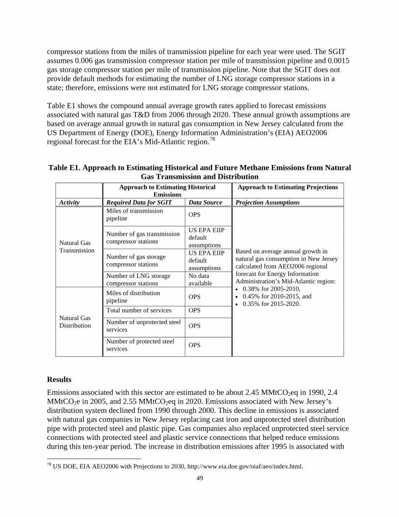
49

compressor stations from the miles of transmission pipeline for each year were used. The SGIT assumes 0.006 gas transmission compressor station per mile of transmission pipeline and 0.0015 gas storage compressor station per mile of transmission pipeline. Note that the SGIT does not provide default methods for estimating the number of LNG storage compressor stations in a state; therefore, emissions were not estimated for LNG storage compressor stations. Table E1 shows the compound annual average growth rates applied to forecast emissions associated with natural gas T&D from 2006 through 2020. These annual growth assumptions are based on average annual growth in natural gas consumption in New Jersey calculated from the US Department of Energy (DOE), Energy Information Administration’s (EIA) AEO2006 regional forecast for the EIA’s Mid-Atlantic region.78

Table E1. Approach to Estimating Historical and Future Methane Emissions from Natural Gas Transmission and Distribution

Approach to Estimating Historical Emissions

Approach to Estimating Projections

Activity Required Data for SGIT Data Source Projection Assumptions Miles of transmission pipeline OPS

Number of gas transmission compressor stations

US EPA EIIP default assumptions

Number of gas storage compressor stations

US EPA EIIP default assumptions

Natural Gas Transmission

Number of LNG storage compressor stations

No data available

Miles of distribution pipeline OPS

Total number of services OPS

Number of unprotected steel services OPS

Natural Gas Distribution

Number of protected steel services OPS

Based on average annual growth in natural gas consumption in New Jersey calculated from AEO2006 regional forecast for Energy Information Administration’s Mid-Atlantic region: • 0.38% for 2005-2010, • 0.45% for 2010-2015, and • 0.35% for 2015-2020.

Results

Emissions associated with this sector are estimated to be about 2.45 MMtCO2eq in 1990, 2.4 MMtCO2e in 2005, and 2.55 MMtCO2eq in 2020. Emissions associated with New Jersey’s distribution system declined from 1990 through 2000. This decline in emissions is associated with natural gas companies in New Jersey replacing cast iron and unprotected steel distribution pipe with protected steel and plastic pipe. Gas companies also replaced unprotected steel service connections with protected steel and plastic service connections that helped reduce emissions during this ten-year period. The increase in distribution emissions after 1995 is associated with 78 US DOE, EIA AEO2006 with Projections to 2030, http://www.eia.doe.gov/oiaf/aeo/index.html.

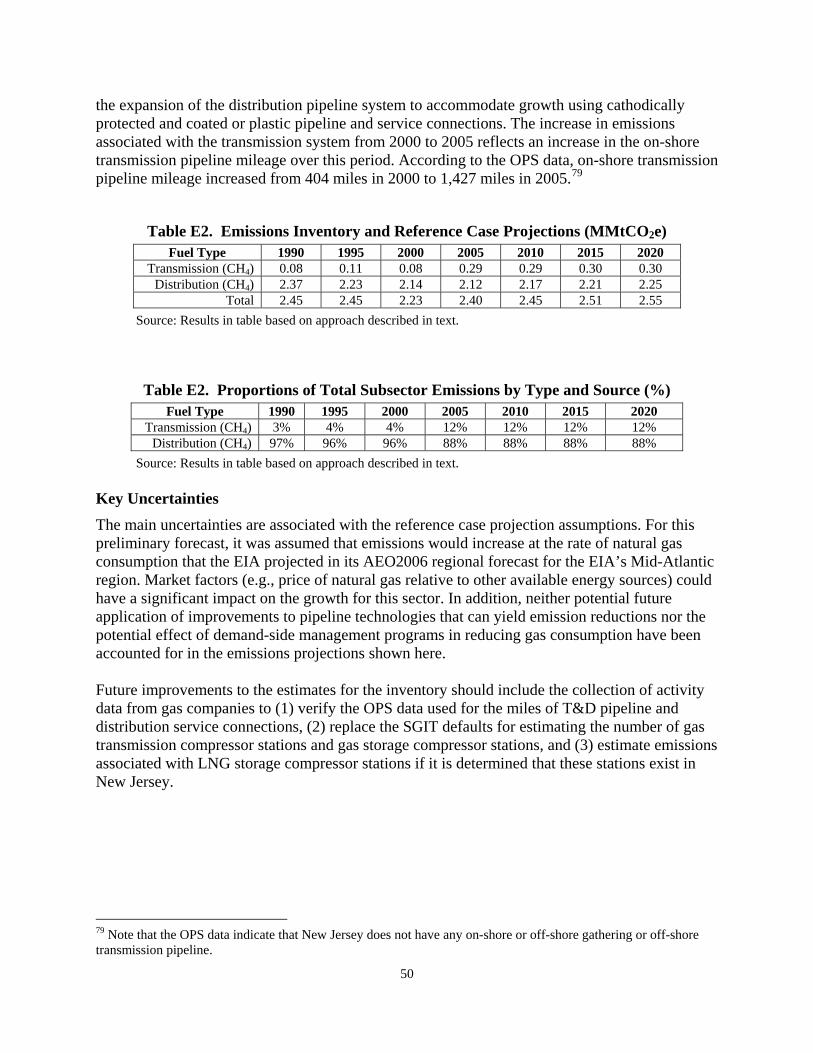
50

the expansion of the distribution pipeline system to accommodate growth using cathodically protected and coated or plastic pipeline and service connections. The increase in emissions associated with the transmission system from 2000 to 2005 reflects an increase in the on-shore transmission pipeline mileage over this period. According to the OPS data, on-shore transmission pipeline mileage increased from 404 miles in 2000 to 1,427 miles in 2005.79

Table E2. Emissions Inventory and Reference Case Projections (MMtCO2e) Fuel Type 1990 1995 2000 2005 2010 2015 2020

Transmission (CH4) 0.08 0.11 0.08 0.29 0.29 0.30 0.30 Distribution (CH4) 2.37 2.23 2.14 2.12 2.17 2.21 2.25

Total 2.45 2.45 2.23 2.40 2.45 2.51 2.55 Source: Results in table based on approach described in text.

Table E2. Proportions of Total Subsector Emissions by Type and Source (%) Fuel Type 1990 1995 2000 2005 2010 2015 2020

Transmission (CH4) 3% 4% 4% 12% 12% 12% 12% Distribution (CH4) 97% 96% 96% 88% 88% 88% 88%

Source: Results in table based on approach described in text. Key Uncertainties The main uncertainties are associated with the reference case projection assumptions. For this preliminary forecast, it was assumed that emissions would increase at the rate of natural gas consumption that the EIA projected in its AEO2006 regional forecast for the EIA’s Mid-Atlantic region. Market factors (e.g., price of natural gas relative to other available energy sources) could have a significant impact on the growth for this sector. In addition, neither potential future application of improvements to pipeline technologies that can yield emission reductions nor the potential effect of demand-side management programs in reducing gas consumption have been accounted for in the emissions projections shown here. Future improvements to the estimates for the inventory should include the collection of activity data from gas companies to (1) verify the OPS data used for the miles of T&D pipeline and distribution service connections, (2) replace the SGIT defaults for estimating the number of gas transmission compressor stations and gas storage compressor stations, and (3) estimate emissions associated with LNG storage compressor stations if it is determined that these stations exist in New Jersey.

79 Note that the OPS data indicate that New Jersey does not have any on-shore or off-shore gathering or off-shore transmission pipeline.

51

Appendix F. Agriculture Overview The emissions discussed in this appendix refer to non-energy methane (CH4) and nitrous oxide (N2O) emissions from enteric fermentation, manure management, and agricultural soils. Emissions and sinks of carbon in agricultural soils are also covered. Energy emissions (combustion of fossil fuels in agricultural equipment) are included in the residential, commercial, and industrial (RCI) sector estimates (see Appendix B). There are two livestock sources of greenhouse gas (GHG) emissions: enteric fermentation and manure management. Methane emissions from enteric fermentation are the result of normal digestive processes in ruminant and non-ruminant livestock. Microbes in the animal digestive system break down food and emit CH4 as a by-product. More CH4 is produced in ruminant livestock because of digestive activity in the large fore-stomach. Methane and N2O emissions from the storage and treatment of livestock manure (e.g., in compost piles or anaerobic treatment lagoons) occur as a result of manure decomposition. The environmental conditions of decomposition drive the relative magnitude of emissions. In general, the more anaerobic the conditions are, the more CH4 is produced because decomposition is aided by CH4 producing bacteria that thrive in oxygen-limited conditions. Under aerobic conditions, N2O emissions are dominant. Emissions estimates from manure management are based on manure that is stored and treated on livestock operations. Emissions from manure that is applied to agricultural soils as an amendment or deposited directly to pasture and grazing land by grazing animals are accounted for in the agricultural soils emissions. The management of agricultural soils can result in N2O emissions and net fluxes of carbon dioxide (CO2) causing emissions or sinks. In general, soil amendments that add nitrogen to soils can also result in N2O emissions. Nitrogen additions drive underlying soil nitrification and de-nitrification cycles, which produce N2O as a by-product. The emissions estimation methodologies used in this inventory account for several sources of N2O emissions from agricultural soils, including decomposition of crop residues, synthetic and organic fertilizer application, manure application, sewage sludge, nitrogen fixation, and histosols (high organic soils, such as wetlands or peatlands) cultivation. Both direct and indirect emissions of N2O occur from the application of manure, fertilizer, and sewage sludge to agricultural soils. Direct emissions occur at the site of application and indirect emissions occur when nitrogen volatilizes or leaches to groundwater or in surface runoff and is transported off-site before entering the nitrification/denitrification cycle. Methane and N2O emissions also result when crop residues are burned and during rice cultivation; however, open burning of crops is prohibited in New Jersey due to air quality concerns and rice is not grown in New Jersey. The net flux of CO2 in agricultural soils depends on the balance of carbon losses from management practices and gains from organic matter inputs to the soil. Carbon dioxide is absorbed by plants through photosynthesis and ultimately becomes the carbon source for organic matter inputs to agricultural soils. When inputs are greater than losses, the soil accumulates carbon and there is a net sink of CO2 into agricultural soils. In addition, soil disturbance from the cultivation of histosols releases large stores of carbon from the soil to the atmosphere. Finally, the practice of adding limestone and dolomite to agricultural soils results in CO2 emissions.

52

The following discusses the data sources, methods, assumptions, and results used to construct the inventory and reference case projections for this sector. The reference case projections assume business-as-usual practices. Emissions and Reference Case Projections (Business-as-Usual)

Methane and Nitrous Oxide GHG emissions for 1990 through 2005 were estimated using the United States Environmental Protection Agency’s (US EPA) State Greenhouse Gas Inventory Tool (SGIT) software and the methods provided in the Emission Inventory Improvement Program (EIIP) guidance document for the sector.80 In general, the SGIT methodology applies emission factors developed for the US to activity data for the agriculture sector. Activity data include livestock population statistics, crop production statistics, amounts of fertilizer applied to crops, and trends in manure management practices. This methodology is based on international guidelines developed by sector experts for preparing GHG emissions inventories.81 The impact of changes in the GWP of methane and nitrous oxide from the most recent IPCC report was assessed and found to be insignificant for this sector, so the original SGIT-based calculations were retained. Defaults in SGIT for New Jersey livestock population and crop production from 1990 to 2005 come from the USDA National Agriculture Statistical Service (NASS).82 These default data were compared to data from New Jersey Department of Agriculture Annual Reports83 and replaced with the local data where differences were found. The default SGIT manure management system assumptions for each livestock category were used for this inventory. SGIT data on fertilizer usage came from Commercial Fertilizers, a report from the Fertilizer Institute. Activity data for fertilizer includes all potential uses in addition to agriculture, such as residential and commercial (e.g., golf courses). The estimates are reported in the agriculture sector but they represent emissions occurring on other land uses. Data were not available to estimate nitrogen released by the cultivation of histosols (i.e., the number of acres of high organic content soils). Given that cultivation of organic soils is a source of CO2 emissions in New Jersey (see below), N2O emissions are also probably occurring. Emissions from enteric fermentation and manure management were projected based on forecasted animal populations. Dairy cattle forecasts were based on state-level projections of

80 GHG emissions were calculated using SGIT, with reference to EIIP, Volume VIII: Chapter 8. “Methods for Estimating Greenhouse Gas Emissions from Livestock Manure Management”, August 2004; Chapter 10. “Methods for Estimating Greenhouse Gas Emissions from Agricultural Soil Management”, August 2004; and Chapter 11. “Methods for Estimating Greenhouse Gas Emissions from Field Burning of Agricultural Residues”, August 2004. 81 Revised 1996 1ntergovermental Panel on Climate Change (IPCC) Guidelines for National Greenhouse Gas Inventories, published by the National Greenhouse Gas Inventory Program of the IPCC, available at (http://www.ipcc-nggip.iges.or.jp/public/gl/invs1.htm; and Good Practice Guidance and Uncertainty Management in National Greenhouse Gas Inventories, published in 2000 by the National Greenhouse Gas Inventory Program of the IPCC, available at: (http://www.ipcc-nggip.iges.or.jp/public/gp/english/). 82 USDA, NASS (http://www.nass.usda.gov/Statistics_by_State/New Jersey/index.asp). 83 Annual Reports, New Jersey Department of Agriculture, http://www.state.nj.us/agriculture/pub/general.html.

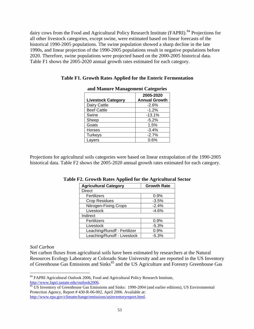
53

dairy cows from the Food and Agricultural Policy Research Institute (FAPRI).84 Projections for all other livestock categories, except swine, were estimated based on linear forecasts of the historical 1990-2005 populations. The swine population showed a sharp decline in the late 1990s, and linear projection of the 1990-2005 populations result in negative populations before 2020. Therefore, swine populations were projected based on the 2000-2005 historical data. Table F1 shows the 2005-2020 annual growth rates estimated for each category.

Table F1. Growth Rates Applied for the Enteric Fermentation

and Manure Management Categories

Livestock Category 2005-2020

Annual GrowthDairy Cattle -2.6% Beef Cattle -1.2% Swine -13.1% Sheep -5.2% Goats 1.5% Horses -3.4% Turkeys -2.7% Layers 0.6%

Projections for agricultural soils categories were based on linear extrapolation of the 1990-2005 historical data. Table F2 shows the 2005-2020 annual growth rates estimated for each category.

Table F2. Growth Rates Applied for the Agricultural Sector Agricultural Category Growth Rate Direct Fertilizers 0.9% Crop Residues -3.5% Nitrogen-Fixing Crops -2.4% Livestock -4.6% Indirect Fertilizers 0.9% Livestock -5.3% Leaching/Runoff - Fertilizer 0.9% Leaching/Runoff - Livestock -5.3%

Soil Carbon Net carbon fluxes from agricultural soils have been estimated by researchers at the Natural Resources Ecology Laboratory at Colorado State University and are reported in the US Inventory of Greenhouse Gas Emissions and Sinks85 and the US Agriculture and Forestry Greenhouse Gas

84 FAPRI Agricultural Outlook 2006, Food and Agricultural Policy Research Institute, http://www.fapri.iastate.edu/outlook2006. 85 US Inventory of Greenhouse Gas Emissions and Sinks: 1990-2004 (and earlier editions), US Environmental Protection Agency, Report # 430-R-06-002, April 2006. Available at: http://www.epa.gov/climatechange/emissions/usinventoryreport.html.

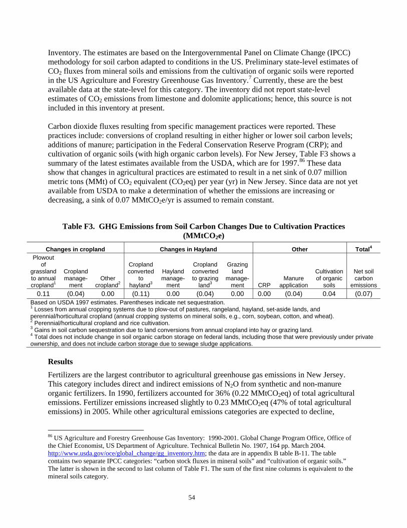
54

Inventory. The estimates are based on the Intergovernmental Panel on Climate Change (IPCC) methodology for soil carbon adapted to conditions in the US. Preliminary state-level estimates of CO2 fluxes from mineral soils and emissions from the cultivation of organic soils were reported in the US Agriculture and Forestry Greenhouse Gas Inventory.7 Currently, these are the best available data at the state-level for this category. The inventory did not report state-level estimates of CO2 emissions from limestone and dolomite applications; hence, this source is not included in this inventory at present. Carbon dioxide fluxes resulting from specific management practices were reported. These practices include: conversions of cropland resulting in either higher or lower soil carbon levels; additions of manure; participation in the Federal Conservation Reserve Program (CRP); and cultivation of organic soils (with high organic carbon levels). For New Jersey, Table F3 shows a summary of the latest estimates available from the USDA, which are for 1997.86 These data show that changes in agricultural practices are estimated to result in a net sink of 0.07 million metric tons (MMt) of CO2 equivalent (CO2eq) per year (yr) in New Jersey. Since data are not yet available from USDA to make a determination of whether the emissions are increasing or decreasing, a sink of 0.07 MMtCO2e/yr is assumed to remain constant.

Table F3. GHG Emissions from Soil Carbon Changes Due to Cultivation Practices (MMtCO2e)

Changes in cropland Changes in Hayland Other Total4 Plowout

of grassland to annual cropland1

Cropland manage-

ment Other

cropland2

Cropland converted

to hayland3

Hayland manage-

ment

Cropland converted to grazing

land3

Grazing land

manage-ment CRP

Manure application

Cultivation of organic

soils

Net soil carbon

emissions 0.11 (0.04) 0.00 (0.11) 0.00 (0.04) 0.00 0.00 (0.04) 0.04 (0.07)

Based on USDA 1997 estimates. Parentheses indicate net sequestration. 1 Losses from annual cropping systems due to plow-out of pastures, rangeland, hayland, set-aside lands, and perennial/horticultural cropland (annual cropping systems on mineral soils, e.g., corn, soybean, cotton, and wheat). 2 Perennial/horticultural cropland and rice cultivation. 3 Gains in soil carbon sequestration due to land conversions from annual cropland into hay or grazing land. 4 Total does not include change in soil organic carbon storage on federal lands, including those that were previously under private ownership, and does not include carbon storage due to sewage sludge applications.

Results Fertilizers are the largest contributor to agricultural greenhouse gas emissions in New Jersey. This category includes direct and indirect emissions of N2O from synthetic and non-manure organic fertilizers. In 1990, fertilizers accounted for 36% (0.22 MMtCO2eq) of total agricultural emissions. Fertilizer emissions increased slightly to 0.23 MMtCO2eq (47% of total agricultural emissions) in 2005. While other agricultural emissions categories are expected to decline,

86 US Agriculture and Forestry Greenhouse Gas Inventory: 1990-2001. Global Change Program Office, Office of the Chief Economist, US Department of Agriculture. Technical Bulletin No. 1907, 164 pp. March 2004. http://www.usda.gov/oce/global_change/gg_inventory.htm; the data are in appendix B table B-11. The table contains two separate IPCC categories: “carbon stock fluxes in mineral soils” and “cultivation of organic soils.” The latter is shown in the second to last column of Table F1. The sum of the first nine columns is equivalent to the mineral soils category.

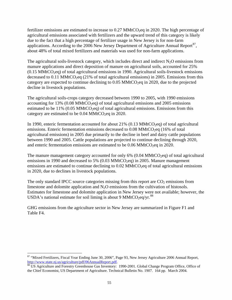
55

fertilizer emissions are estimated to increase to 0.27 MMtCO2eq in 2020. The high percentage of agricultural emissions associated with fertilizers and the upward trend of this category is likely due to the fact that a high percentage of fertilizer usage in New Jersey is for non-farm applications. According to the 2006 New Jersey Department of Agriculture Annual Report87, about 48% of total mixed fertilizers and materials was used for non-farm applications. The agricultural soils-livestock category, which includes direct and indirect N2O emissions from manure applications and direct deposition of manure on agricultural soils, accounted for 25% (0.15 MMtCO2eq) of total agricultural emissions in 1990. Agricultural soils-livestock emissions decreased to 0.11 MMtCO2eq (21% of total agricultural emissions) in 2005. Emissions from this category are expected to continue declining to 0.05 MMtCO2eq in 2020, due to the projected decline in livestock populations. The agricultural soils-crops category decreased between 1990 to 2005, with 1990 emissions accounting for 13% (0.08 MMtCO2eq) of total agricultural emissions and 2005 emissions estimated to be 11% (0.05 MMtCO2eq) of total agricultural emissions. Emissions from this category are estimated to be 0.04 MMtCO2eq in 2020. In 1990, enteric fermentation accounted for about 21% (0.13 MMtCO2eq) of total agricultural emissions. Enteric fermentation emissions decreased to 0.08 MMtCO2eq (16% of total agricultural emissions) in 2005 due primarily to the decline in beef and dairy cattle populations between 1990 and 2005. Cattle populations are projected to continue declining through 2020, and enteric fermentation emissions are estimated to be 0.06 MMtCO2eq in 2020. The manure management category accounted for only 6% (0.04 MMtCO2eq) of total agricultural emissions in 1990 and decreased to 5% (0.03 MMtCO2eq) in 2005. Manure management emissions are estimated to continue declining to 0.02 MMtCO2eq of total agricultural emissions in 2020, due to declines in livestock populations. The only standard IPCC source categories missing from this report are CO2 emissions from limestone and dolomite application and N2O emissions from the cultivation of histosols. Estimates for limestone and dolomite application in New Jersey were not available; however, the USDA’s national estimate for soil liming is about 9 MMtCO2eq/yr.88 GHG emissions from the agriculture sector in New Jersey are summarized in Figure F1 and Table F4.

87 “Mixed Fertilizers, Fiscal Year Ending June 30, 2006”, Page 93, New Jersey Agriculture 2006 Annual Report, http://www.state.nj.us/agriculture/pdf/06AnnualReport.pdf. 88 US Agriculture and Forestry Greenhouse Gas Inventory: 1990-2001. Global Change Program Office, Office of the Chief Economist, US Department of Agriculture. Technical Bulletin No. 1907. 164 pp. March 2004.

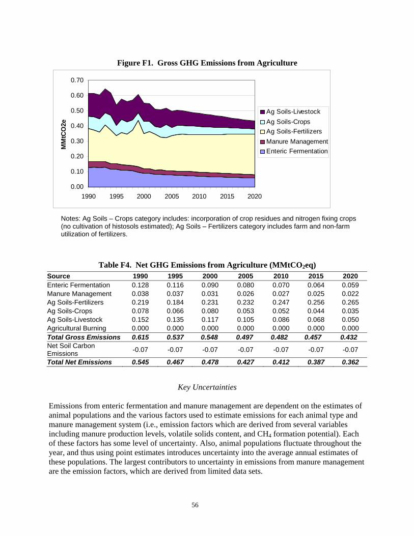
56

Figure F1. Gross GHG Emissions from Agriculture

0.00

0.10

0.20

0.30

0.40

0.50

0.60

0.70

1990 1995 2000 2005 2010 2015 2020

MM

tCO

2e

Ag Soils-LivestockAg Soils-CropsAg Soils-FertilizersManure ManagementEnteric Fermentation

Notes: Ag Soils – Crops category includes: incorporation of crop residues and nitrogen fixing crops (no cultivation of histosols estimated); Ag Soils – Fertilizers category includes farm and non-farm utilization of fertilizers.

Table F4. Net GHG Emissions from Agriculture (MMtCO2eq) Source 1990 1995 2000 2005 2010 2015 2020 Enteric Fermentation 0.128 0.116 0.090 0.080 0.070 0.064 0.059 Manure Management 0.038 0.037 0.031 0.026 0.027 0.025 0.022 Ag Soils-Fertilizers 0.219 0.184 0.231 0.232 0.247 0.256 0.265 Ag Soils-Crops 0.078 0.066 0.080 0.053 0.052 0.044 0.035 Ag Soils-Livestock 0.152 0.135 0.117 0.105 0.086 0.068 0.050 Agricultural Burning 0.000 0.000 0.000 0.000 0.000 0.000 0.000 Total Gross Emissions 0.615 0.537 0.548 0.497 0.482 0.457 0.432 Net Soil Carbon Emissions -0.07 -0.07 -0.07 -0.07 -0.07 -0.07 -0.07

Total Net Emissions 0.545 0.467 0.478 0.427 0.412 0.387 0.362

Key Uncertainties

Emissions from enteric fermentation and manure management are dependent on the estimates of animal populations and the various factors used to estimate emissions for each animal type and manure management system (i.e., emission factors which are derived from several variables including manure production levels, volatile solids content, and CH4 formation potential). Each of these factors has some level of uncertainty. Also, animal populations fluctuate throughout the year, and thus using point estimates introduces uncertainty into the average annual estimates of these populations. The largest contributors to uncertainty in emissions from manure management are the emission factors, which are derived from limited data sets.

57

As mentioned above, for emissions associated with changes in agricultural soil carbon levels, the only data currently available are for 1997. When newer data are released by the USDA, these should be reviewed to represent current conditions as well as to assess trends. In particular, given the potential for some CRP acreage to retire and possibly return to active cultivation prior to 2020, the emissions could be appreciably affected. As mentioned above, emission estimates for soil liming and cultivation of histosols have not been developed for New Jersey. Another contributor to the uncertainty in the emission estimates is the projection assumptions. The growth rates for most source categories are based on the assumption that the average annual rate of change in future year emissions will follow the historical average annual rate of change from 1990 through 2005.

58

Appendix G. Waste Management Overview Greenhouse gas (GHG) emissions from waste management include:

• Solid waste management – methane (CH4) emissions from municipal and industrial solid waste landfills, accounting for CH4 that is flared or captured for energy production (this includes both open and closed landfills);

• Solid waste combustion – CH4, carbon dioxide (CO2), and nitrous oxide (N2O) emissions from the combustion of solid waste in incinerators or waste to energy plants or during open burning; and

• Wastewater management – CH4 and N2O from municipal wastewater and CH4 from industrial wastewater (WW) treatment facilities.

The following discusses the data sources, methods, assumptions, and results used to construct the inventory and reference case projections for this sector. The reference case projections assume business-as-usual practices.

Inventory and Reference Case Projections (Business-as-Usual)

Solid Waste Management For solid waste management, emissions were calculated using the United States Environmental Protection Agency’s (US EPA) AP-42 equation,89 which is used by EPA’s Landfill Gas Emissions Model (LandGEM). Also used were NJDEP data on annual waste emplacement, estimated age of waste in place, and landfill gas management methods. .The GWP of methane was set at 25 to be consistent with most recent IPCC report.90 There are 100 relatively large landfills in New Jersey representing both open and closed landfills. Twenty-one of these sites collect landfill gas either for direct use as gas or to produce electricity. Another 14 sites collect landfill gas with an active collection system and flare it. The remaining 65 sites are uncontrolled or passively vented. Table G1 provides a listing of sites that are controlled. There are some additional CH4 emissions from the approximately 300 landfills that are too small and old to be listed individually. NJDEP extrapolated a best-fitting exponential trend line of a plot of landfill volume versus estimated methane emissions data, which suggested that the total methane emissions from these landfills is no more than 5,000 metric tons/year.

89 As per EPA’s AP-42 Section on Municipal Solid Waste Landfills: http://www.epa.gov/ttn/chief/ap42/ch02/final/c02s04.pdf. 90 IPCC, 2007.

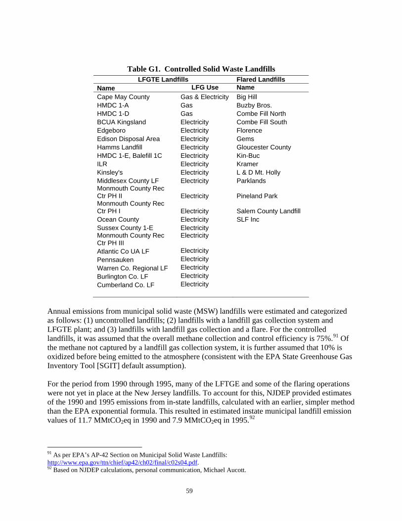
59

Table G1. Controlled Solid Waste Landfills LFGTE Landfills Flared Landfills

Name LFG Use Name Cape May County Gas & Electricity Big Hill HMDC 1-A Gas Buzby Bros. HMDC 1-D Gas Combe Fill North BCUA Kingsland Electricity Combe Fill South Edgeboro Electricity Florence Edison Disposal Area Electricity Gems Hamms Landfill Electricity Gloucester County HMDC 1-E, Balefill 1C Electricity Kin-Buc ILR Electricity Kramer Kinsley's Electricity L & D Mt. Holly Middlesex County LF Electricity Parklands Monmouth County Rec Ctr PH II Electricity Pineland Park Monmouth County Rec Ctr PH I Electricity Salem County Landfill Ocean County Electricity SLF Inc Sussex County 1-E Electricity Monmouth County Rec Ctr PH III

Electricity

Atlantic Co UA LF Electricity Pennsauken Electricity Warren Co. Regional LF Electricity Burlington Co. LF Electricity Cumberland Co. LF Electricity

Annual emissions from municipal solid waste (MSW) landfills were estimated and categorized as follows: (1) uncontrolled landfills; (2) landfills with a landfill gas collection system and LFGTE plant; and (3) landfills with landfill gas collection and a flare. For the controlled landfills, it was assumed that the overall methane collection and control efficiency is 75%.91 Of the methane not captured by a landfill gas collection system, it is further assumed that 10% is oxidized before being emitted to the atmosphere (consistent with the EPA State Greenhouse Gas Inventory Tool [SGIT] default assumption). For the period from 1990 through 1995, many of the LFTGE and some of the flaring operations were not yet in place at the New Jersey landfills. To account for this, NJDEP provided estimates of the 1990 and 1995 emissions from in-state landfills, calculated with an earlier, simpler method than the EPA exponential formula. This resulted in estimated instate municipal landfill emission values of 11.7 MMtCO2eq in 1990 and 7.9 MMtCO2eq in 1995.92

91 As per EPA’s AP-42 Section on Municipal Solid Waste Landfills: http://www.epa.gov/ttn/chief/ap42/ch02/final/c02s04.pdf. 92 Based on NJDEP calculations, personal communication, Michael Aucott.

60

In addition to the in-state landfills, New Jersey exports a significant amount of waste for disposal out-of-state. NJDEP data on the amount of waste disposed of in-state and the amount disposed of out-of-state from 1985 through 200493 was used. NJDEP data on amount of waste incinerated was also used.94 To estimate the amount of in-state waste incinerated in each remaining year from 1990 through 2004, the ratio of the tons of waste incinerated in-state in 2003 to the total tons of waste disposed of in-state in 2003 was multiplied by the total amount of waste disposed of in-state in the selected year. The CO2 emissions from the active in-state landfills for each year from 1990 through 2004 were then totaled. To estimate the emissions from the waste generated in New Jersey, but exported out-of-state, these emissions from active in-state landfills were then multiplied by the ratio of the tons of waste disposed of out-of-state in a given year to the tons of waste landfilled in-state in that same year (total tons of waste disposed of in-state minus the calculated tons of waste incinerated). Reference case projections of emissions from landfills were based on the same equations used to calculate the base inventory, with waste continuing to be emplaced at the landfills that are currently active (as of 2006). The ratio of the tons of waste from New Jersey landfilled out-of-state to the tons of waste landfilled in-state was assumed to remain at the 2004 level (the latest year for which these data were available) of 1.15 tons of waste landfilled out-of-state for every ton of waste landfilled in-state through the year 2020. The calculation of emissions from this waste disposed of out-of-state for the reference case projections was performed in the same manner as the calculation of emissions from out-of-state waste disposal used in the base inventory. The SGIT default was used for industrial solid waste landfills. This default is based on national data indicating that industrial landfilled waste is emplaced at approximately 7% of the rate of MSW emplacement. We assumed that this additional industrial waste emplacement occurs beyond that already addressed in the emplacement rates for MSW sites described above. Due to a lack of data, no controls were assumed for industrial waste landfills. Emissions from industrial landfills from 2007 through 2020 were calculated using the same rate of 7% of the uncontrolled MSW emissions in each of the reference case projection years. Solid Waste Combustion NJDEP throughput data for the five municipal waste combustion facilities currently operating in New Jersey (Camden, Essex, Gloucester, Union, and Warren Counties) was used.95 Emissions from these waste combustion facilities are captured under the electricity production sector as these are all waste-to-energy facilities. Therefore, emissions from solid waste combustion are listed as 0 for the waste sector.

93 “New Jersey Solid Waste Database Trends Analysis: 1985 through 2004 (millions of tons per year),” http://www.state.nj.us/dep/dshw/recycling/05_trends.pdf. 94 Michael Aucott, New Jersey Department of Environmental Protection, spreadsheet MSW_incin_calcs.xls, provided to Maureen Mullen, CCS, August 9, 2007. 95 Michael Aucott, New Jersey Department of Environmental Protection.

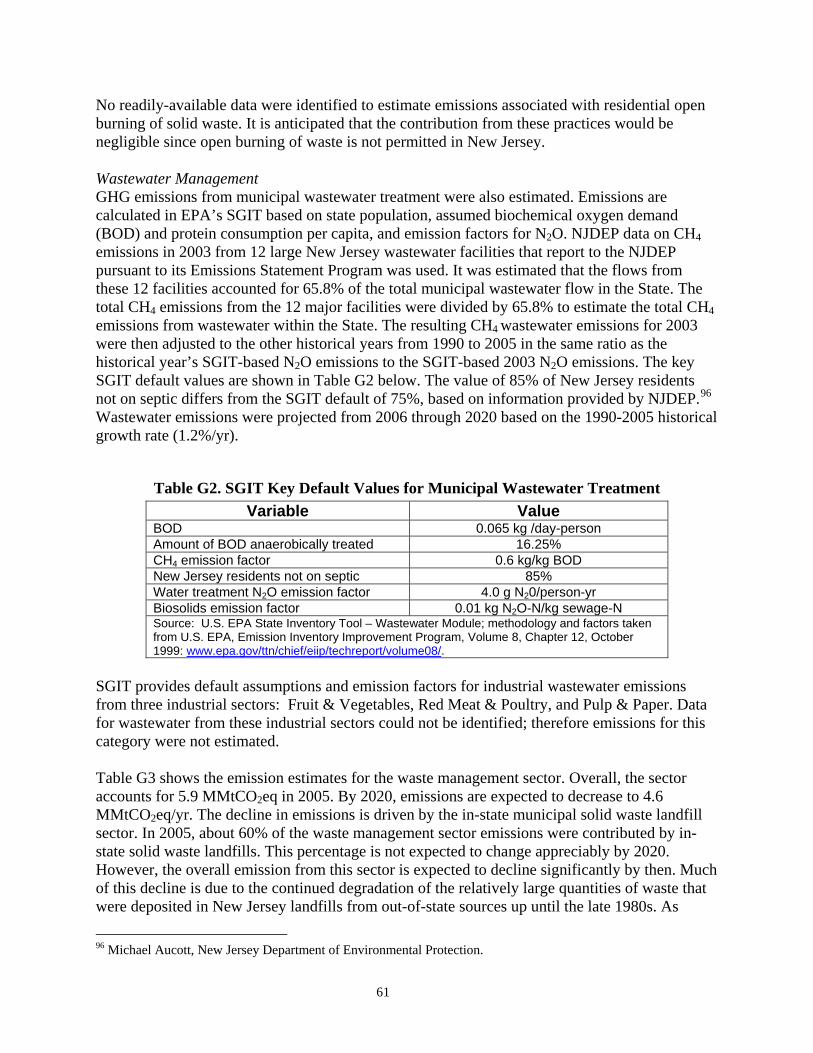
61

No readily-available data were identified to estimate emissions associated with residential open burning of solid waste. It is anticipated that the contribution from these practices would be negligible since open burning of waste is not permitted in New Jersey. Wastewater Management GHG emissions from municipal wastewater treatment were also estimated. Emissions are calculated in EPA’s SGIT based on state population, assumed biochemical oxygen demand (BOD) and protein consumption per capita, and emission factors for N2O. NJDEP data on CH4 emissions in 2003 from 12 large New Jersey wastewater facilities that report to the NJDEP pursuant to its Emissions Statement Program was used. It was estimated that the flows from these 12 facilities accounted for 65.8% of the total municipal wastewater flow in the State. The total CH4 emissions from the 12 major facilities were divided by 65.8% to estimate the total CH4 emissions from wastewater within the State. The resulting CH4 wastewater emissions for 2003 were then adjusted to the other historical years from 1990 to 2005 in the same ratio as the historical year’s SGIT-based N2O emissions to the SGIT-based 2003 N2O emissions. The key SGIT default values are shown in Table G2 below. The value of 85% of New Jersey residents not on septic differs from the SGIT default of 75%, based on information provided by NJDEP.96 Wastewater emissions were projected from 2006 through 2020 based on the 1990-2005 historical growth rate (1.2%/yr).

Table G2. SGIT Key Default Values for Municipal Wastewater Treatment Variable Value

BOD 0.065 kg /day-person Amount of BOD anaerobically treated 16.25% CH4 emission factor 0.6 kg/kg BOD New Jersey residents not on septic 85%

Water treatment N2O emission factor 4.0 g N20/person-yr Biosolids emission factor 0.01 kg N2O-N/kg sewage-N Source: U.S. EPA State Inventory Tool – Wastewater Module; methodology and factors taken from U.S. EPA, Emission Inventory Improvement Program, Volume 8, Chapter 12, October 1999: www.epa.gov/ttn/chief/eiip/techreport/volume08/.

SGIT provides default assumptions and emission factors for industrial wastewater emissions from three industrial sectors: Fruit & Vegetables, Red Meat & Poultry, and Pulp & Paper. Data for wastewater from these industrial sectors could not be identified; therefore emissions for this category were not estimated. Table G3 shows the emission estimates for the waste management sector. Overall, the sector accounts for 5.9 MMtCO2eq in 2005. By 2020, emissions are expected to decrease to 4.6 MMtCO2eq/yr. The decline in emissions is driven by the in-state municipal solid waste landfill sector. In 2005, about 60% of the waste management sector emissions were contributed by in-state solid waste landfills. This percentage is not expected to change appreciably by 2020. However, the overall emission from this sector is expected to decline significantly by then. Much of this decline is due to the continued degradation of the relatively large quantities of waste that were deposited in New Jersey landfills from out-of-state sources up until the late 1980s. As

96 Michael Aucott, New Jersey Department of Environmental Protection.

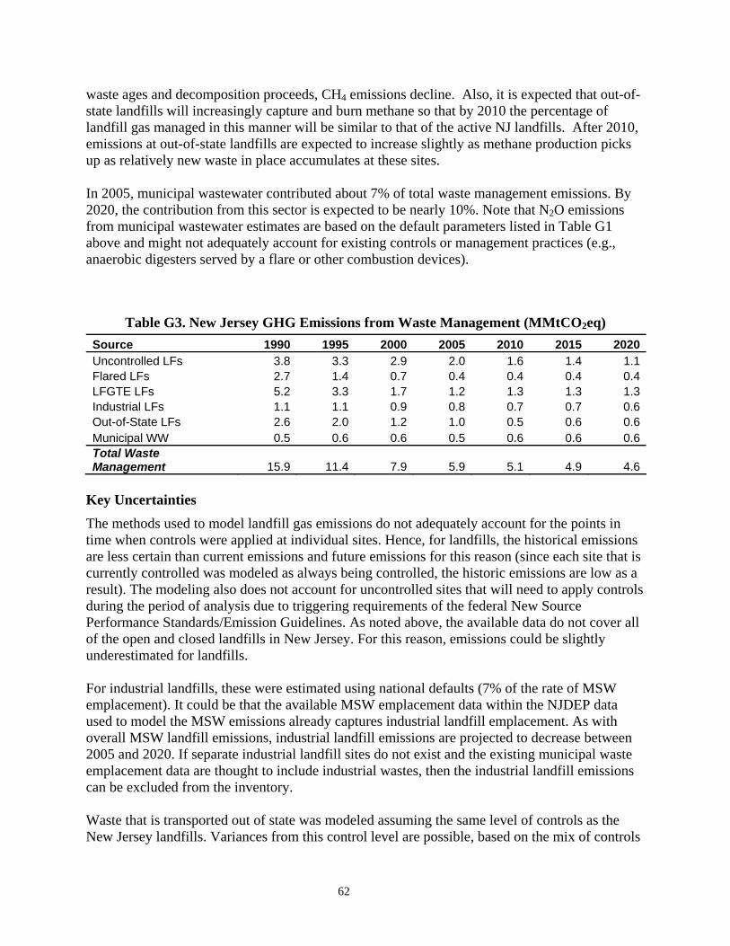
62

waste ages and decomposition proceeds, CH4 emissions decline. Also, it is expected that out-of-state landfills will increasingly capture and burn methane so that by 2010 the percentage of landfill gas managed in this manner will be similar to that of the active NJ landfills. After 2010, emissions at out-of-state landfills are expected to increase slightly as methane production picks up as relatively new waste in place accumulates at these sites. In 2005, municipal wastewater contributed about 7% of total waste management emissions. By 2020, the contribution from this sector is expected to be nearly 10%. Note that N2O emissions from municipal wastewater estimates are based on the default parameters listed in Table G1 above and might not adequately account for existing controls or management practices (e.g., anaerobic digesters served by a flare or other combustion devices).

Table G3. New Jersey GHG Emissions from Waste Management (MMtCO2eq) Source 1990 1995 2000 2005 2010 2015 2020Uncontrolled LFs 3.8 3.3 2.9 2.0 1.6 1.4 1.1Flared LFs 2.7 1.4 0.7 0.4 0.4 0.4 0.4LFGTE LFs 5.2 3.3 1.7 1.2 1.3 1.3 1.3Industrial LFs 1.1 1.1 0.9 0.8 0.7 0.7 0.6Out-of-State LFs 2.6 2.0 1.2 1.0 0.5 0.6 0.6Municipal WW 0.5 0.6 0.6 0.5 0.6 0.6 0.6Total Waste Management 15.9 11.4 7.9 5.9 5.1 4.9 4.6

Key Uncertainties The methods used to model landfill gas emissions do not adequately account for the points in time when controls were applied at individual sites. Hence, for landfills, the historical emissions are less certain than current emissions and future emissions for this reason (since each site that is currently controlled was modeled as always being controlled, the historic emissions are low as a result). The modeling also does not account for uncontrolled sites that will need to apply controls during the period of analysis due to triggering requirements of the federal New Source Performance Standards/Emission Guidelines. As noted above, the available data do not cover all of the open and closed landfills in New Jersey. For this reason, emissions could be slightly underestimated for landfills.

For industrial landfills, these were estimated using national defaults (7% of the rate of MSW emplacement). It could be that the available MSW emplacement data within the NJDEP data used to model the MSW emissions already captures industrial landfill emplacement. As with overall MSW landfill emissions, industrial landfill emissions are projected to decrease between 2005 and 2020. If separate industrial landfill sites do not exist and the existing municipal waste emplacement data are thought to include industrial wastes, then the industrial landfill emissions can be excluded from the inventory. Waste that is transported out of state was modeled assuming the same level of controls as the New Jersey landfills. Variances from this control level are possible, based on the mix of controls

63

used by the receiving landfills. This analysis also assumed that the share of the State’s waste disposed of out-of-state remains constant in the future. It should be noted that, some GHG inventories for other states receiving waste from New Jersey will include these emissions within that state’s inventory as well97. As noted, emissions from residential open burning (e.g. in backyard burn barrels) are not included. While the additional emissions are likely to be small, estimates can be made if open burning activity data are identified.

For the wastewater sector, the key uncertainties are associated with the application of SGIT default values for the parameters listed in Table G1 above (e.g., fraction of BOD which is anaerobically decomposed). The SGIT defaults were derived from national data. As described above, data were not available to estimate emissions from the industrial wastewater treatment sector. If these data are identified (either production volumes in each industry or wastewater flow & chemical oxygen demand estimates), then emission estimates can be derived.

97 The emissions associated with NJ waste will only be included in another state’s inventory if it uses historical data on total amounts of waste deposited in the state. If instead a state uses the SGIT default approach, its CH4 emissions from landfills will be estimated using population and national per capita estimates of amount of waste landfilled, and thus will not capture the emissions associated with waste imported from NJ or elsewhere.

64

Appendix H. Forestry and Land-Use Change Overview Forestland emissions refer to the net carbon dioxide (CO2) flux98 from forested lands in New Jersey, which account for about 40% of the state’s land area.99 The dominant forest type in New Jersey is Oak-Hickory which makes up about 46% of forested lands. Other common forest types are Loblolly-Shortleaf Pine (30%) and Oak-Gum-Cypress, Maple-Beech-Birch, and Oak-Pine, which make up less than 10% each. Through photosynthesis, carbon dioxide is taken up by trees and plants and converted to carbon in biomass within the forests. Carbon dioxide emissions occur from respiration in live trees, decay of dead biomass, and fires. Carbon is also stored in the associated soils. In addition, carbon is stored for long time periods when forest biomass is harvested for use in durable wood products. Carbon dioxide flux is the net balance of carbon dioxide removals from and emissions to the atmosphere from the processes described above. Emissions of carbon dioxide occur from the loss of forests and other vegetated lands when these are cleared for construction of buildings, parking lots, etc.100 Estimates of these emissions of carbon dioxide can be combined with estimates of the net carbon dioxide flux from forested and other vegetated lands to develop a combined estimate of the overall net carbon dioxide flux associated with land-use and land-use change. The following discusses the data sources, methods, assumptions, and results used to construct the inventory and reference case projections from forestry and land-use change. The reference case projections assume business-as-usual practices. Emissions and Reference Case Projections (Business-as-Usual) There are two methods that have been used as part of this project to estimate the net flux of carbon dioxide associated with forest growth. Method 1 This approach makes use of the carbon online estimator (COLE),101 and couples this with statewide estimates of different types of land cover. COLE was used by the New Jersey Department of Environmental Protection (NJDEP) to develop an estimate that, statewide, an average of 4.8 metric tons (Mt) of carbon dioxide equivalents (CO2e) are sequestered per hectare

98 “Flux” refers to both emissions of CO2 to the atmosphere and removal (sinks) of CO2 from the atmosphere. 99 Total forested acreage is 1.92 million acres in 2004; J. Smith, USFS, personal communication with S. Roe, CCS, April 2007. Acreage by forest type available from the USFS at: http://www.fs.fed.us/ne/global/pubs/books/epa/states/NJ.htm. The total land area in New Jersey is 4.75 million acres (http://www.50states.com/newjerse.htm). 100 It is assumed herein that these emissions are associated with a non-sustainable loss of biomass, although in some cases, e.g. residential developments, trees are replanted and their growth will sequester carbon 101 http://ncasi.uml.edu/COLE/

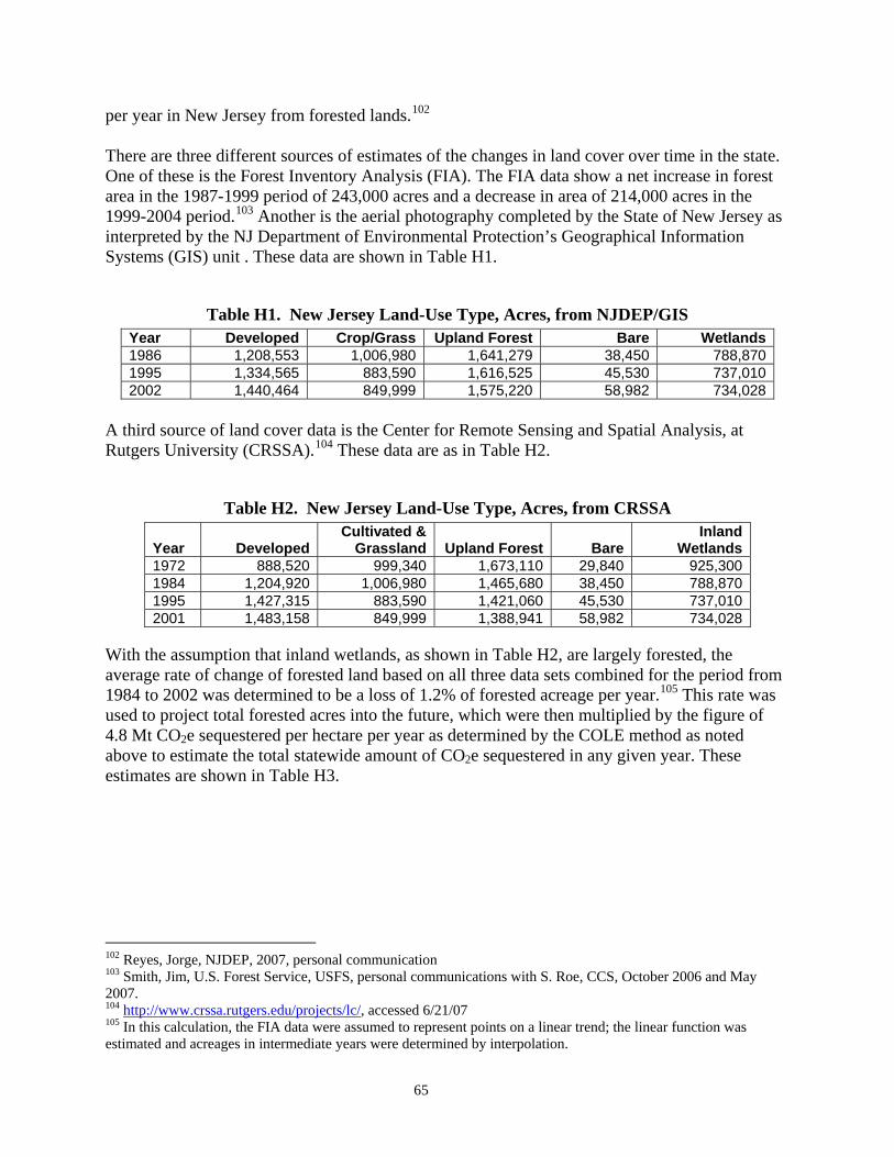
65

per year in New Jersey from forested lands.102 There are three different sources of estimates of the changes in land cover over time in the state. One of these is the Forest Inventory Analysis (FIA). The FIA data show a net increase in forest area in the 1987-1999 period of 243,000 acres and a decrease in area of 214,000 acres in the 1999-2004 period.103 Another is the aerial photography completed by the State of New Jersey as interpreted by the NJ Department of Environmental Protection’s Geographical Information Systems (GIS) unit . These data are shown in Table H1.

Table H1. New Jersey Land-Use Type, Acres, from NJDEP/GIS Year Developed Crop/Grass Upland Forest Bare Wetlands1986 1,208,553 1,006,980 1,641,279 38,450 788,8701995 1,334,565 883,590 1,616,525 45,530 737,0102002 1,440,464 849,999 1,575,220 58,982 734,028

A third source of land cover data is the Center for Remote Sensing and Spatial Analysis, at Rutgers University (CRSSA).104 These data are as in Table H2.

Table H2. New Jersey Land-Use Type, Acres, from CRSSA

Year Developed Cultivated &

Grassland Upland Forest BareInland

Wetlands1972 888,520 999,340 1,673,110 29,840 925,3001984 1,204,920 1,006,980 1,465,680 38,450 788,8701995 1,427,315 883,590 1,421,060 45,530 737,0102001 1,483,158 849,999 1,388,941 58,982 734,028

With the assumption that inland wetlands, as shown in Table H2, are largely forested, the average rate of change of forested land based on all three data sets combined for the period from 1984 to 2002 was determined to be a loss of 1.2% of forested acreage per year.105 This rate was used to project total forested acres into the future, which were then multiplied by the figure of 4.8 Mt CO2e sequestered per hectare per year as determined by the COLE method as noted above to estimate the total statewide amount of CO2e sequestered in any given year. These estimates are shown in Table H3.

102 Reyes, Jorge, NJDEP, 2007, personal communication 103 Smith, Jim, U.S. Forest Service, USFS, personal communications with S. Roe, CCS, October 2006 and May 2007. 104 http://www.crssa.rutgers.edu/projects/lc/, accessed 6/21/07 105 In this calculation, the FIA data were assumed to represent points on a linear trend; the linear function was estimated and acreages in intermediate years were determined by interpolation.

66

Table H3. Method 1 Estimated CO2 Equivalent Sequestration, New Jersey

Year Millions of Metric Tons CO2 Equivalent Sequestered per Year

1990 7.81 1995 7.37 2000 6.95 2005 6.55 2010 6.18 2015 5.83 2020 5.50

Releases of carbon from the loss of forests and other vegetated lands when these are cleared for construction of buildings, parking lots, etc. were estimated based on several data sources as approximately 95 Mt per acre.106 When converted to CO2e107, and multiplied by one half of the estimated increase in developed area per year determined from the NJDEP GIS and CRSSA data (with the assumption that half of the land converted to developed land each year was originally forested), a statewide total CO2 equivalent release of approximately 1.1 million metric tons (MMt) per year throughout the 1984 to 2002 period was estimated. Method 2

This approach relied on NJDEP/GIS land-use data (Table H1) and relevant default assumptions108 about the quantity of stored carbon for each land-use type, including associated soil carbon. It also took into consideration the carbon remaining in harvested wood products. Carbon remains stored in the durable wood products109 pool or is transferred to landfills where much of the carbon remains stored over a long period of time. With this method, the amount of land remaining in each land-use type and also the amount of land lost from each land type110 was multiplied by factors based on the quantity assumptions listed above including annual biomass growth and soil density increase. Overall total net quantities of the equivalent CO2 sequestered for the periods 1986 to 1995 and 1995 to 2002 were estimated to be 6.18 MMt tons per year for the first period and 5.93 MMt per year for the second period.

106 These include the following: 1), the default value from the Intergovernmental Panel on Climate Change (IPCC) of 87.5 to 125 metric tons carbon/ha (based on a dry matter/ha estimate from this source, and with the assumption that the dry matter is 50% carbon); 2), calculations by Jorge Reyes, NJDEP which result in a figure of 96 metric tons carbon/ha; 3), Table A-191 from Annex 3 of the USEPA’s 2007 Draft Greenhouse Gas Emissions inventory, which indicates that above-ground matter in the Northeastern U.S. forests contains about 103 metric tons carbon/ha, 4) an estimate by Ed Lempicki, NJDEP Division of Forestry, that there are 80 tons of biomass material per acre, which, , converts to 98 metric tons carbon/ha; and 5), 107 Based on the following conversion: MTCO2 = MTC x 3.66 108 Adapted from IPCC and other sources: [a] Biomass carbon density: 38 metric tons (Mt)/acre (forest), 4 Mt/acre (grassland), 2 Mt/acre (bare land), 1.2 Mt/acre (cropland); [b] soil carbon density: 8 Mt/acre (bare land) and 24 Mt/acre (froest land); [c] biomass density increase: 1% per year; [d] soil carbon density increase: 1% per year; and [e] amount of carbon stored in forest products: 12 Mt/acre. 109 We estimate 50% of forest removal converted to wood products. Factor used to convert wood volume to weight: 3 pounds per board foot. 110 In the absence of default factors for wetlands, we assumed them to be 50% forested and 50% bare.

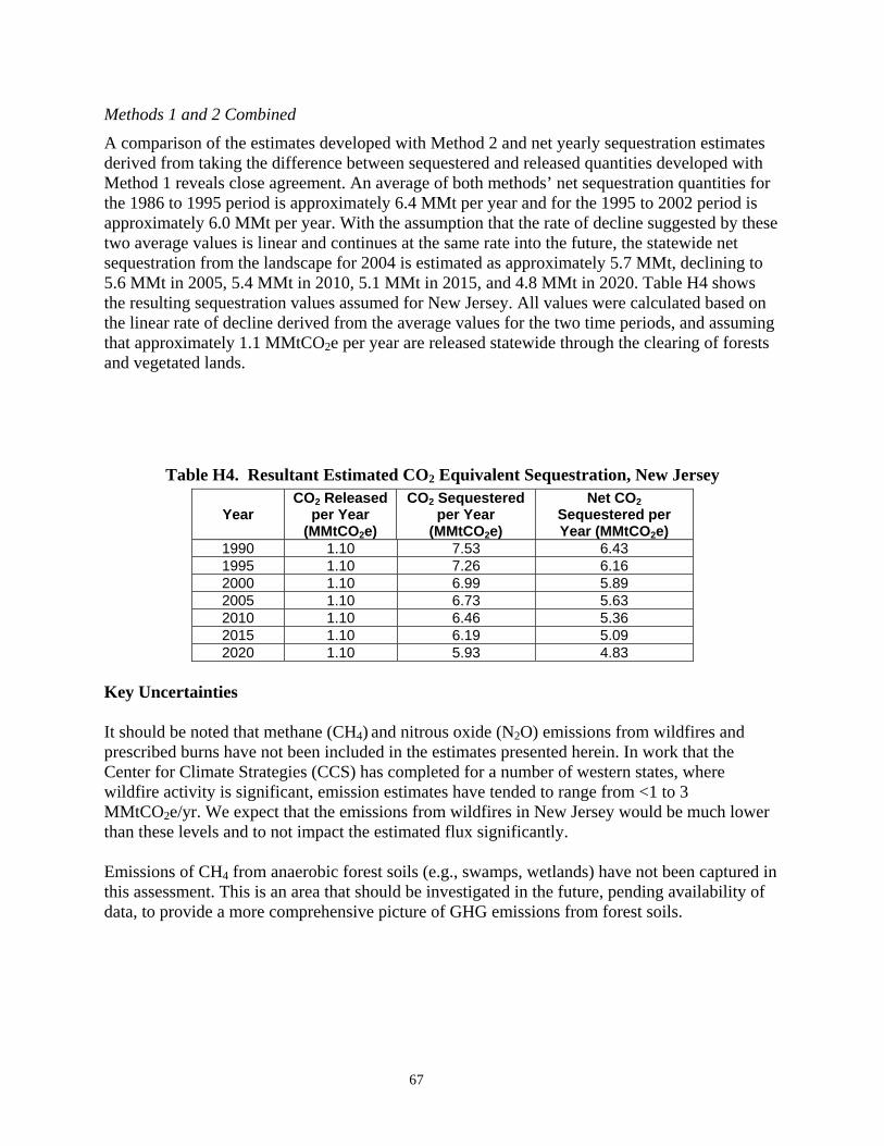
67

Methods 1 and 2 Combined

A comparison of the estimates developed with Method 2 and net yearly sequestration estimates derived from taking the difference between sequestered and released quantities developed with Method 1 reveals close agreement. An average of both methods’ net sequestration quantities for the 1986 to 1995 period is approximately 6.4 MMt per year and for the 1995 to 2002 period is approximately 6.0 MMt per year. With the assumption that the rate of decline suggested by these two average values is linear and continues at the same rate into the future, the statewide net sequestration from the landscape for 2004 is estimated as approximately 5.7 MMt, declining to 5.6 MMt in 2005, 5.4 MMt in 2010, 5.1 MMt in 2015, and 4.8 MMt in 2020. Table H4 shows the resulting sequestration values assumed for New Jersey. All values were calculated based on the linear rate of decline derived from the average values for the two time periods, and assuming that approximately 1.1 MMtCO2e per year are released statewide through the clearing of forests and vegetated lands.

Table H4. Resultant Estimated CO2 Equivalent Sequestration, New Jersey

Year CO2 Released

per Year (MMtCO2e)

CO2 Sequestered per Year

(MMtCO2e)

Net CO2 Sequestered per Year (MMtCO2e)

1990 1.10 7.53 6.43 1995 1.10 7.26 6.16 2000 1.10 6.99 5.89 2005 1.10 6.73 5.63 2010 1.10 6.46 5.36 2015 1.10 6.19 5.09 2020 1.10 5.93 4.83

Key Uncertainties It should be noted that methane (CH4) and nitrous oxide (N2O) emissions from wildfires and prescribed burns have not been included in the estimates presented herein. In work that the Center for Climate Strategies (CCS) has completed for a number of western states, where wildfire activity is significant, emission estimates have tended to range from <1 to 3 MMtCO2e/yr. We expect that the emissions from wildfires in New Jersey would be much lower than these levels and to not impact the estimated flux significantly. Emissions of CH4 from anaerobic forest soils (e.g., swamps, wetlands) have not been captured in this assessment. This is an area that should be investigated in the future, pending availability of data, to provide a more comprehensive picture of GHG emissions from forest soils.

68

Appendix I. Responses to Comments on Draft Inventory Responses to comments on the DRAFT New Jersey Greenhouse Gas Inventory and Reference Case Projections 1990-2020 The DEP received a number of comments on the DRAFT New Jersey Greenhouse Gas Inventory and Reference Case Projections 1990-2020 (Inventory) that was released in February, 2008. To the extent feasible, these comments have been addressed and changes made as necessary to the final version of the Inventory. The important comments and the DEP’s responses are summarized below. In some cases, several individual comments with similar or identical points are summarized and included as one comment. 1) Comment: Future inventories should include separate greenhouse gas (GHG) emissions quantities for specific sectors, sub-sectors, or even specific facilities. Response: The DEP concurs, and, to the extent that such data are available will make these data available in future inventories. 2) Comment: The assumption noted in the Inventory that all electric power generated in New Jersey is consumed in New Jersey is incorrect. Response: The DEP agrees that some of the electric power generated in New Jersey is consumed out-of-state. However, the Inventory is based on the net quantity of imported electricity, which is determined by the difference between the power consumed in the state vs. the power produced in the state. The DEP recognizes that differences between the overall rate of GHG emissions per units of power produced between imported power and in-state power introduces a potential source of uncertainty or error in GHG emissions estimates that should be attributed to NJ, and it intends to investigate this issue further as the Inventory is updated. 3) Comment: Appendix A does not include a discussion of key uncertainties as are presented for the other sectors. It is also not clear that the Inventory takes into account the substantial variation in the CO2 intensity among different electricity generating units. Response: A discussion of the uncertainties in emissions estimates associated with electricity production has been added to the chapter (Appendix A) of the Inventory. Clearly there are also major uncertainties associated with prediction of future electricity use and the associated emissions. In the final version of the Inventory, the DEP relied on projections from the NJ Board of Public Utilities (BPU). It is expected that these projections will be continually re-evaluated as better data become available. The 2004 numbers in the Inventory are based on data on fuel consumed by in-state facilities, and on an aggregate estimate of the amount of GHG emissions associated with net imported power, so an assessment of the CO2 intensity of different generating units was not necessary.

69

4) Comment: The emissions projections are not consistent with some other projections available. Response: The DEP has reviewed some data regarding projections that were submitted, and has found no reason to change the projections in the Inventory, except that the electric power projections have been changed to conform to the BPU’s estimates. The DEP acknowledges that all projections as far into the future as 2020 are uncertain, and will attempt to improve these projections as newer and better data become available. 5) Comment: The 2005 sulfur hexafluoride (SF6) estimate appears to be low, based on data provided by the commenter on one power provider’s estimated releases. Response: The DEP has revised the 2005 estimate slightly to be in conformance with the data provided. 6) Comment: Natural gas emissions in 2020 are not likely to be similar to or slightly higher than 2004 and 2005 estimates as shown in the Inventory. Response: In the absence of data sufficient to determine the likely trend in these emissions, the DEP has not revised the projections in the Inventory. As better data become available, the DEP hopes to revise these projections. 7) Comment: The projections of VMT growth are unrealistically low, and it is overly optimistic to assume that the California low emissions vehicle (CALEV) requirements will be implemented in NJ soon. Response: It is true that the rate of VMT growth since 1990 has been higher than the approximately 1% per year growth assumed in the projections of on-road transportation emissions for 2020. However, the long-term growth (since 1960) has been closer to 1% than to the recent trend of approximately 2%. Again, as with other sectors, the DEP will revisit projections as better data become available. The DEP is operating under the assumption that the CALEV provisions that apply to GHGs will in fact be implemented in NJ in a timely manner. 8) Comment: The most recent global warming potential (GWP) value for methane as provided in the most recent IPCC report, which is 25 (for a 100-year time horizon), should be used. Further, the DEP should consider using the 20-year time horizon, which would place a higher value on near-term reductions of methane. Response: The DEP concurs that the most recent GWP value for methane should be used. The carbon dioxide equivalent emissions associated with for methane in the final version of the inventory for all but those sectors with relatively trivial emissions of methane have been revised upward to reflect this new value. However, the DEP has chosen to stick with the 100-year time horizon for methane to be consistent with the GHG inventories of other municipalities, states, and nations.

70

9) Comment: The DEP should not include emissions associated with the combustion of imported municipal solid waste (MSW). Response: The DEP will consider this point in future inventories. However, it is expected that the impact of the current inclusion of imported waste in the total MSW quantities will be small. 10) Comment: New data indicate that the portion of paper and other biofuels in MSW is higher than the default calculation parameters made available by EPA as used in the Inventory, and also that the default N2O emissions calculation methods are incorrect, with the result that the GHG emissions associated with MSW combustion are too high by nearly a factor of two. Response: The DEP has reviewed the data provided and finds that the comment has validity and calls for further review and the acquisition of more data. If warranted, the estimates from this sector will be revised in the future. 11) Comment: The Inventory over-estimates the landfill gas collection efficiency, does not recognize the destruction efficiency of landfill gas by flares, and over-estimates the actual effectiveness of soil oxidation. Response: There appears to be considerable uncertainty regarding both the effectiveness of soil oxidation and the gas collection efficiency at landfills. However, regarding the latter, the DEP is aware that some data indicate that in fact the 75% gas collection efficiency used in the Inventory may be an underestimate and that some landfills may collect 90% or more of the gas. And, contrary to the comment, the presence of gas flares and also the combustion of gas by some landfills for the production of energy were fully considered in the development of the estimate. For these reasons, the DEP does not contemplate changing the methodology for the estimation of emissions from the landfill sector at this time. In this final version of the Inventory, however, updated information on the amount of waste disposed at certain NJ landfills and of the presence of flares and energy recovery was used resulting in revisions of the emissions estimates. Also, as noted in another response above, the GWP of methane has been changed to 25, which also affects the emissions from this sector.