Neutrino oscillations: Perspective of long-baseline experiments

Neutrino Oscillations
November 25, 2020
Contents
1 Introduction 3
2 Neutrino Flavour Oscillation in Words 3
3 Evidence for Neutrino Flavour Oscillations 53.1 Solar Neutrinos and the Solar Neutrino Problem . . . . . . . . . . . . . . . . . . . . . 5
3.1.1 What you should know . . . . . . . . . . . . . . . . . . . . . . . . . . . . . . . 93.2 Atmospheric Neutrinos and the Atmospheric Neutrino Anomaly . . . . . . . . . . . . 10
3.2.1 Atmospheric Neutrino Detectors and the Atmospheric Neutrino Anomaly . . . 103.2.2 What you should know . . . . . . . . . . . . . . . . . . . . . . . . . . . . . . . 13
4 Two Flavour Neutrino Oscillation Theory 134.1 What you should know . . . . . . . . . . . . . . . . . . . . . . . . . . . . . . . . . . . 17
5 Interpretation of the Atmospheric Neutrino Problem 175.1 Accelerator Verification . . . . . . . . . . . . . . . . . . . . . . . . . . . . . . . . . . . 185.2 The T2K Experiment . . . . . . . . . . . . . . . . . . . . . . . . . . . . . . . . . . . . 205.3 Verification that the atmospheric oscillations are mostly νµ → ντ . . . . . . . . . . . . 215.4 What you should know . . . . . . . . . . . . . . . . . . . . . . . . . . . . . . . . . . . 22
6 Interpretation of the Solar Neutrino Data 236.1 Matter effects . . . . . . . . . . . . . . . . . . . . . . . . . . . . . . . . . . . . . . . . 23
6.1.1 Observations . . . . . . . . . . . . . . . . . . . . . . . . . . . . . . . . . . . . 266.1.2 Solar Results . . . . . . . . . . . . . . . . . . . . . . . . . . . . . . . . . . . . 27
6.2 Verification of the solar oscillation parameters . . . . . . . . . . . . . . . . . . . . . . 286.3 What you should know . . . . . . . . . . . . . . . . . . . . . . . . . . . . . . . . . . . 29
7 Three Neutrino Oscillations 307.1 How to measure θ13 . . . . . . . . . . . . . . . . . . . . . . . . . . . . . . . . . . . . . 34
7.1.1 C,P and T violation . . . . . . . . . . . . . . . . . . . . . . . . . . . . . . . . 357.2 The measurement of θ13 . . . . . . . . . . . . . . . . . . . . . . . . . . . . . . . . . . 37
7.2.1 T2K Returns . . . . . . . . . . . . . . . . . . . . . . . . . . . . . . . . . . . . 387.3 What you need to know . . . . . . . . . . . . . . . . . . . . . . . . . . . . . . . . . . 39
1

8 Summary of Current Knowledge and open questions 398.1 Open Questions . . . . . . . . . . . . . . . . . . . . . . . . . . . . . . . . . . . . . . . 398.2 What you should know . . . . . . . . . . . . . . . . . . . . . . . . . . . . . . . . . . . 40
9 A Spanner In The Works? 409.1 LSND . . . . . . . . . . . . . . . . . . . . . . . . . . . . . . . . . . . . . . . . . . . . 40
9.1.1 Combining with other experiments . . . . . . . . . . . . . . . . . . . . . . . . 429.1.2 The miniBooNE Experiment . . . . . . . . . . . . . . . . . . . . . . . . . . . . 43
9.2 The Reactor and Gallium Anomalies . . . . . . . . . . . . . . . . . . . . . . . . . . . 449.3 What you should know . . . . . . . . . . . . . . . . . . . . . . . . . . . . . . . . . . . 45
10 The Future 4510.1 Degeneracies . . . . . . . . . . . . . . . . . . . . . . . . . . . . . . . . . . . . . . . . . 4610.2 Current and future experiments . . . . . . . . . . . . . . . . . . . . . . . . . . . . . . 4610.3 Mass hierarchy measurements . . . . . . . . . . . . . . . . . . . . . . . . . . . . . . . 4710.4 Measuring δCP . . . . . . . . . . . . . . . . . . . . . . . . . . . . . . . . . . . . . . . 4910.5 What you need to know . . . . . . . . . . . . . . . . . . . . . . . . . . . . . . . . . . 51
2

1 Introduction
This section discusses the phenomenon of neutrino flavour oscillations, the big discovery of the last10 years, which prompted the first major change to the standard model in the last 20 years. We willdiscuss the evidence for neutrino oscillations, look at the formalism - both for 2-flavour and 3-flavouroscillations, and look at oscillation experiments.
This is a long document - where possible I will try to point out what you should know and whatyou don’t necessarily need for an exam.
2 Neutrino Flavour Oscillation in Words
I will first introduce the concept of neutrino flavour oscillations without going into the rigorous theory(see below). We have seen that the thing we call a neutrino is a state that is produced in a weakinteraction. It is, by definition, a flavour eigenstate, in the sense that a neutrino is always producedwith, or absorbed to give, a charged lepton of electron, muon or tau flavour. The neutrino that isgenerated with the charged electron is the electron neutrino, and so on. However, as with the quarksand the CKM matrix, it is possible that the flavour eigenstates (states with definite flavour) are notidentical to the mass eigenstates (states which have definite mass).
What does this mean? Suppose we label the mass states as ν1, ν2 and ν3 and that they havedifferent, but close, masses. Everytime we create an electron in a weak interaction we will create oneof these mass eigenstates (ensuring the energy and momentum is conserved at the weak interactionvertex as we do so). Suppose that we create these with different probabilities (i.e. 10% of the timewe create a ν1 etc). If we could resolve the mass of each state, we could follow each mass state as itpropagates. However, the neutrino masses are too small to experimentally resolve them. We knowwe created one of them, but not which one, so what we create, at the weak interaction vertex, is acoherent superposition of the νi mass states - this coherent superposition we call the electron neutrino:
|νe >= Ue1|ν1 > +Ue2|ν2 > +Ue3|ν3 > (1)
If this is the case, the following can happen : suppose one generates a neutrino at a source. Thisneutrino will have definite flavour, but will be produced as a linear combination of states of definitemass. The states of definite mass will propagate out of the source towards the detector. If the stateshave different masses, then the phase between the states will change with distance from the source(we will make this clear soon). At the detector, the mass states will have different relative phases tothose the mass states had at the source, and when we go to detect them, it is possible that we willdetect a flavour state which was not present in the beam to begin with. If one restricts oneself totwo-flavour oscillations, we find that the probability of starting with one flavour, say να, at the sourcebut detecting another, say νβ, at the detector is
P (να → νβ) = sin2(2θ)sin2(1.27∆m2 L(km)
E(GeV )) (2)
This equation has a number of points of interest
• The angle θ: this is the so-called mixing angle. It defines how different the flavour states arefrom the mass states. If θ=0, the flavour states are identical to the mass states (that is, the ναwill propagate from source to detector as a να with definite momentum. Clearly in this case,
3
oscillations cannot happen. If θ = π4
then the oscillations are said to be maximal and at somepoint along the path between source and detector all of the να we started with will oscillate toνβ.
• The mass squared difference, ∆m2 : If there are 2 flavours there will be 2 mass states.This parameter is the difference in squared masses of each of these states : ∆m2 = m2
1 −m22.
For neutrino oscillations to occur, at least one of the mass states must be non-zero. This simplestatement has huge implications - for oscillations to happen, the neutrino must have mass.Furthur the masses of the mass states must be different, else ∆m2 = 0 and P (να → νβ) = 0.You can see why this is : the masses control the relative phase of the two mass wavefunctions.If they are the same, then the mass states will never get out of phase and you will measure thesame linear combination of mass states at the detector as you generated at the source. Notealso the limitation of neutrino oscillation experiments - they can give us detailed informationon the difference between the mass values, but cannot tell us what the absolute mass of thestates are. Neither can they tell us whether m1 is larger in mass than m2. If ∆m2 → −∆m2
the probability will still be the same.
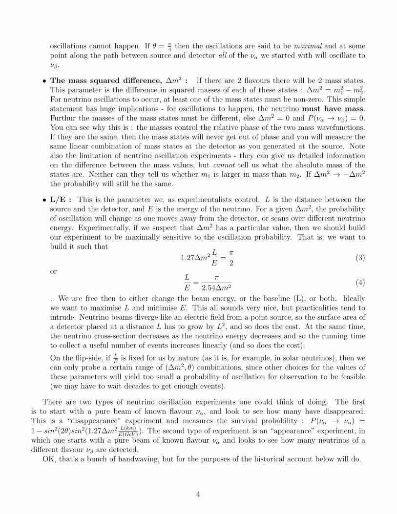
• L/E : This is the parameter we, as experimentalists control. L is the distance between thesource and the detector, and E is the energy of the neutrino. For a given ∆m2, the probabilityof oscillation will change as one moves away from the detector, or scans over different neutrinoenergy. Experimentally, if we suspect that ∆m2 has a particular value, then we should buildour experiment to be maximally sensitive to the oscillation probability. That is, we want tobuild it such that
1.27∆m2 L
E=π
2(3)
orL
E=
π
2.54∆m2(4)
. We are free then to either change the beam energy, or the baseline (L), or both. Ideallywe want to maximise L and minimise E. This all sounds very nice, but practicalities tend tointrude. Neutrino beams diverge like an electric field from a point source, so the surface area ofa detector placed at a distance L has to grow by L2, and so does the cost. At the same time,the neutrino cross-section decreases as the neutrino energy decreases and so the running timeto collect a useful number of events increases linearly (and so does the cost).
On the flip-side, if LE
is fixed for us by nature (as it is, for example, in solar neutrinos), then wecan only probe a certain range of (∆m2, θ) combinations, since other choices for the values ofthese parameters will yield too small a probability of oscillation for observation to be feasible(we may have to wait decades to get enough events).
There are two types of neutrino oscillation experiments one could think of doing. The firstis to start with a pure beam of known flavour να, and look to see how many have disappeared.This is a “disappearance” experiment and measures the survival probability : P (να → να) =
1− sin2(2θ)sin2(1.27∆m2 L(km)E(GeV )
). The second type of experiment is an “appearance” experiment, inwhich one starts with a pure beam of known flavour να and looks to see how many neutrinos of adifferent flavour νβ are detected.
OK, that’s a bunch of handwaving, but for the purposes of the historical account below will do.
4

3 Evidence for Neutrino Flavour Oscillations
3.1 Solar Neutrinos and the Solar Neutrino Problem
We discussed solar neutrino generation in the previous handout. The solar neutrino flux derived fromBahcall’s Standard Solar Model is shown in Figure 1 for reference.
The Standard Solar Model predicts that most of the flux comes from the pp neutrinos withenergies below 0.4 MeV. Only the Gallium experiements are sensitive to this component. The Chlorineexperiments can just observe part of the 7Be line, and can see the other components. The big waterexperiments (Super-Kamiokande, SNO) can only view the 8B neutrinos as they have too high athreshold to see below about 5 MeV.
Figure 1: The Standard Solar Model prediction of the solar neutrino flux. Thresholds for each ofthe solar experiments is shown at the top. SuperK and SNO are only sensitive to Boron-8 and hepneutrinos. The gallium experiments have the lowest threshold and can observe pp neutrinos.
Homestake
Ray Davis’ Homestake experiment was the first neutrino experiment designed to look for solarneutrinos. It started in 1965, and after several years of running produced a result for the averagecapture rate of solar neutrinos of 2.56±0.25 SNU (remember that 1 SNU = 10−36 neutrino interactionsper target atom per second). The big surprise was that the Standard Solar Models of the timepredicted that Homestake should have seen about 8.1 ± 1.2 SNU, over three times larger than themeasured rate. This discrepancy became known as the Solar Neutrino Problem.
At the time it was assumed that something was wrong with the experiment. After all, the Home-stake experiment is based on counting very low rate interactions. How did they know that they wereseeing solar neutrinos at all? They had no directional or energy information. The objections towardsthe experiment became harder to maintain when the Super-Kamiokande results were released.
5

Super-Kamiokande
The main mode of solar neutrino detection in Super-Kamiokande is the elastic scattering channelνe+e
− → νe+e− which has a threshold of 5 MeV. This threshold comes from the design of the detector
- neutrinos with energies less than 5 MeV which elastically scatter in the water will not generate anelectron with enough momentum to be seen in the detector. Super-Kamiokande observed a capturerate of about 0.45±0.02 SNU, with a model prediction of 1.0±0.2 SNU, almost a factor of two largerthan observation. In addition, since Super-Kamiokande was able to reconstruct the direction of theincoming electron (with some large resolution due to both scattering kinematics - Super-Kamiokandesees the final state electron which isn’t quite collinear with the incoming neutrino direction - and tomultiple scattering of the final state electron - which smears the directional resolution out even more),it was able to show that the electron neutrinos do indeed come from the sun (see Figure 2).
Figure 2: The cosine of the angle between the measured electron in the Super-Kamiokande solarneutrino data, and the direction to the sun at the time the event occurred. A clear peak can be seenfor cosθ > 0.5 above an essentially flat background. The peak is broad because of kinematic smearingand multiple scattering of the final state electron in the water.
SAGE and GALLEX
An obvious drawback of both the Chlorine and the water experiments was that they were onlysensitive to the relatively rare 8B and pep neutrinos.The Gallium experiments were able to observepart of the bulk pp neutrino flux. SAGE, which ran with 50 tonnes of Gallium, observed a capturerate of 70.8± 5.0 SNU compared to a model prediction of 129± 9 SNU. It’s counterpart, GALLEX,observed a rate of 77.5 ± 8 SNU. Again the observations were lower than the prediction - this timeby about 40%. This is, in itself, important as it shows that deficit is energy dependent.
A summary of these results is shown in Figure 3.In all experiments, the model seems to overestimate the solar neutrino capture rate by approxi-
mately a factor of two although, crucially, the discrepancy appears to be energy dependent - the lowerin energy the experiment is able to probe, the less the discrepancy. Such a discrepancy has two main
6

Figure 3: The state of the solar neutrino problem before SNO. Each group of bars represents a differenttype of experiment : Chlorine on the left, water in the middle and Gallium on the right. The bluebars in each cluster represent the measurements of individual experiments, in SNUs. The middle barshows the Standard Solar Model prediction. In all cases, the measurements are less than predicted.
solutions. One is that our model of the Sun is just wrong, and the other is that there is somethingwrong with the neutrinos coming from the sun.
It is now believed that Bahcall’s Standard Solar Model (SSM) describes the sun well. This is largelyon the basis of data obtained from studies of helioseismology - or sun quakes. Helioseismology utilizeswaves that propagate throughout the Sun to measure the invisible internal structure and dynamicsof a star. There are millions of distinct, resonating, sound waves, seen by the doppler shifting oflight emitted at the Sun’s surface. The periods of these waves depend on their propagation speedsand the depths of their resonant cavities, and the large number of resonant modes, with differentcavities, allows us to construct extremely narrow probes of the temperature, chemical composition,and motions from just below the surface down to the very core of the Sun. The SSM predicts thevelocity of sound waves in the Sun as a function of radial distance out from the core. This is shownin Figure 4. The model agrees with measured data to better than 1.0%. Since these sound speedsdepend very much on the chemical composition and structure of the star, which are predictions fromthe SSM, the model is regarded as reliable. Certainly there is no way that one could tweak the modelto remove up to 50% of the neutrino output whilst leaving all other observables unaffected.
In order to show that neutrino flavour oscillations are the cause of the Solar Neutrino Problem,it is necessary to be able to observe the solar flux in a way that is independent of neutrino flavour.All solar experiments detect solar neutrinos through charged current interactions in the detector :νe + X → e− + Y . The radiochemical experiments used the charged current interaction to generatethe unstable ion, whereas the water Cerenkov experiments needed the final state electron as a tagthat a νe had interacted in the detector. This immediately creates a problem - solar neutrino energiesare less than about 30 MeV, whereas the charged muon mass is 105 MeV. In order to interact viathe charged current there must be sufficient energy available to create the charged leptons. From thepoint of view of all the solar experiments, electron neutrinos might well be changing to muon or tau
7

Figure 4: The speed of sound waves in the Sun as a function of radial distance from the solar corefor a set of models of solar composition. The graph shows the fractional difference of the SSM fromhelioseismological data (Serenelli, arXiv:1601.07179 [astro-ph.SR]). Regardless of choice, the modeldeviates from measurement by less than 1%.
neutrinos, but as there is not enough energy to create the respective charged lepton, and as all theexperiments relied on that charged current interaction to detect the neutrino, all experiments justwouldn’t be able to see the νµ or ντ part of the flux. What was needed was a way to measure thetotal neutrino flux, regardless of flavour. This was finally provided by the SNO detector.
The SNO experiment used a tank of heavy water as its target. Heavy water consists of D2O withthe deuteron containing a proton and a neutron, rather than just a proton (as in Hydrogen). Theimportant point is that the deuteron is a very fragile nucleus. It only takes about 2 MeV to breakit apart into a proton and a neutron. Solar neutrinos have energies up to 30 MeV and so any of theneutrino νe, νµ or ντ can break apart a deuteron in a neutral current interaction. SNO was able todetect the final state neutron and so all those neutrinos that weren’t visible to the radiochemical orwater Cerenkov experiments are visible to SNO. In fact, SNO was able to detect neutrino via threedifferent, and redundant, interactions:
• The Elastic Scattering (ES) channel :
ν + e− → ν + e− (5)
This is the same sort of interaction used by Super–Kamiokande. Electron neutrinos can, how-ever, interact via both the charged and neutral currents (draw some Feynman diagrams toconvince yourself of this), whereas νµ and ντ neutrinos interact only via the neutral current atthese energies (due to the final lepton mass threshold). Elastic scattering probes a combinationof the electron, muon and tau neutrino flux given by
φ(νe) + 0.15(φ(νµ) + φ(ντ )) (6)
• The Charged Current (CC) channel :
νe + d→ p+ p+ e− (7)
8

This reaction can only be initiated by electron neutrinos and therefore only measure φ(νe).SNO used this channel to ensure that it was seeing the same reduction in νe rate as observed inprevious solar neutrino experiments.
• The Neutral Current (NC) channel :
ν + d→ n+ p+ ν (8)
This is the important reaction. It measure the total flux : φ(νe)+φ(νµ)+φ(ντ ). The experimentalchallenge is to measure that final state neutron. SNO did this 3 different ways as cross checkson their final result.
Using the measurement of the three independent reaction channels, SNO was able to disentan-gle the individual fluxes of neutrinos. Their measurement of the neutrino fluxes was, in units of10−8cm−2s−1,
φCC = φ(νe) = 1.76± 0.01
φES = φ(νe) + 0.15(φ(νµ) + φ(ντ )) = 2.39± 0.26
φNC = φ(νe) + φ(νµ) + φ(ντ ) = 5.09± 0.63
The numbers are striking. The total flux of muon and tau neutrinos from the Sun (φ(νµ) +φ(ντ ))is (3.33±0.63)×10−8cm−2s−1, roughly 3 times larger than the flux of νe. Since we know the Sun onlyproduces electron neutrinos, the only conclusion we can draw is that neutrinos must change flavourbetween the Sun and the Earth. Furthur, the SSM predicts a total flux of neutrinos with energiesgreater than 2 MeV (the deuteron break-up energy) of
φSSM = (5.05± 1.01)× 10−8cm−2s−1 (9)
which is in very good agreement with the NC flux measured by SNO. Here endeth the Solar NeutrinoProblem. Previous experiments were seeing less electron neutrino than predicted, because two-thirdsof the electron neutrinos were changing flavour on the way from the sun to the earth. The total fluxis predicted well by the SSM.
3.1.1 What you should know
• What the solar neutrino problem was, including the specific experiments that were involved(Homestake, Gallex, Super–Kamiokande, SNO)
• Why neither the solar model, or details of the specific experiment could account for the solarneutrino problem, and why the phenomenon of neutrino flavour oscillation could.
• How SNO definitively solved the solar neutrino problem
9

3.2 Atmospheric Neutrinos and the Atmospheric Neutrino Anomaly
The atmosphere is constantly being bombarded by cosmic rays. These are composed of protons(95%), alpha particles (5%) and heavier nuclei and electrons (< 1%). When the primary cosmic rayshit nuclei in the atmosphere they shower, setting up a cascade of hadrons. The atmospheric neutrinosstem from the decay of these hadrons during flight. The dominant part of the decay chain is
π+ → µ+νµ µ+ → e+νeνµ (10)
π− → µ−νµ µ− → e−νeνµ (11)
At higher energies, one also begins to see neutrinos from kaon decay as well. In general the spectrumof these neutrinos peaks at 1 GeV and extends up to hundreds of GeV. At moderate energies one cansee that the ratio
R =(νµ + νµ)
(νe + νe)(12)
should be equal to 2. In fact, computer models of the entire cascade process predict this ratio to beequal to 2 with a 5% uncertainty. The total flux of atmospheric neutrinos, however, has an uncertaintyof about 20% due to various assumptions in the models.
A detector looking at atmospheric neutrinos is, necessarily, positioned on (or just below) theEarth’s surface (see Figure 5). Flight distances for neutrinos detected in these experiments can thusvary from 15 km for neutrinos coming down from an interaction above the detector, to more than13,000 km for neutrinos coming from interactions in the atmosphere below the detector on the otherside of the planet.
3.2.1 Atmospheric Neutrino Detectors and the Atmospheric Neutrino Anomaly
There have been effectively two categories of detectors used to study atmospheric neutrinos - waterCerenkov detectors and tracking calorimeters. Of the former, the most influential has been Super-Kamiokande (again). We will not discuss the latter.
Atmospheric neutrino experiments measure two quantities : the ratio of νµ to νe observed in theflux, and zenith angle distribution of the neutrinos (that is, the path length distribution). To helpinterpret the results and to cancel systematic uncertainties most experiments report a double ratio
R =(Nµ/Ne)DATA(Nµ/Ne)SIM
(13)
where Nµ is the number of νµ events which interacted in the detector (called “muon-like”) and Ne
is the number of νe events which interacted (called “electron-like”). The ratio of NµNe
is measured inthe data and is also measured in a computational model of the experiment, which incorporates allknown physics of atmospheric neutrino production, neutrino propagation to the detector and detectorresponse. The absolute flux predictions largely cancel in this double ratio. If the observed flavourcomposition agrees with expectation that R = 1.
A compilation of R values from a number of different experiments is shown in Table 1. With theexception of Frejus, all measurements of R are significantly less than 1, indicating that either therewas less νµ in the data than in the prediction, or there was more νe, or both. This became known asthe Atmospheric Neutrino Anomaly.
In addition to low values ofR, Super-Kamiokande was able to measure the direction of the incomingneutrinos. Neutrinos are produced everywhere in the atmosphere and can reach the detector from all
10

Figure 5: A diagram of an atmospheric neutrino experiment. A detector near the surface sees neutrinosthat travel about 15 km looking up, while neutrinos arriving at the detector from below can travelup to 13,000 km. This distance is measured by the “zenith angle”; the polar angle as measured fromthe vertical direction at the detector : cosθzen = 1 is for neutrinos coming directly down, whereascosθzen = −1 describes upwards-going neutrinos.
directions. In principle, we expect the flux of neutrinos to be isotropic - the same number comingdown as going up. The zenith angle distributions from Super-Kamiokande are shown in Figure 6.In this figure, the left column shows the νe (“e-like”) events, where as the right column depicts νµevents. The top and middle rows show low energy events where the neutrino energy was less than 1GeV, whilst the bottom row shows events where the neutrino energy was greater than 1 GeV. Thered line shows what should be expected from standard cosmic ray models and the black points showwhat Super-Kamiokande actually measured. Clearly, whilst the electron-like data agrees reasonablywell with expectation, the muon-like data deviates significantly. At low energies appoximately halfof the νµ are missing over the full range of zenith angles. At high energy the number of νµ comingdown from above the detector seems to agree with expectation, but half of the same νµ coming upfrom below the detector are missing.
Experiment Type of experiment RSuper-Kamiokande Water Cerenkov 0.675± 0.085
Soudan2 Iron Tracking Calorimeter 0.69± 0.13IMB Water Cerenkov 0.54± 0.12
Kamiokande Water Cerenkov 0.60± 0.07Frejus Iron Tracking Calorimeter 1.0± 0.15
Table 1: Measurements of the double ratio for various atmospheric neutrino experiments.
11

Figure 6: Zenith angle distributions of νµ and νe-initiated atmospheric neutrino events detected bySuper-Kamiokande. The left column shows the νe (“e-like”) events, where as the right column depictsνµ events. The top and middle rows show low energy events where the neutrino energy was less than1 GeV, whilst the bottom row shows events where the neutrino energy was greater than 1 GeV. Thered line shows what should be expected from standard cosmic ray models and the black points showwhat Super-Kamiokande actually measured.
12

These results are reasonably easy to explain within the context of flavour oscillations. Neutrinosarriving at the Super-Kamiokande detector at different zenith angles have travelled anywhere from 15km (for neutrinos coming straight down) to 13000 km (for neutrinos coming straight up). Referringback to the oscillation probability in Equation 4, we see that if ∆m2 ∼ 10−3eV2 and the neutrinoenergy is about 10 GeV, then for neutrinos coming down the oscillation probability will be roughlyzero, whereas for neutrinos coming up, the oscillation probability will be roughly 1
2sin2(2θ) (where the
factor of 0.5 comes from averaging the kinematic factor, sin2(1.27∆m2L/E), over many oscillationperiods). Furthur, the fact that νµ neutrinos are reduced, but the electron neutrinos are not enhancedsuggests that the dominant oscillation mode for the atmospheric neutrinos is νµ → ντ . UnfortunatelySuper-Kamiokande cannot easily detect ντ interactions and can’t check this option itself.
Both the solar and atmospheric neutrino problems can be explained by neutrino flavour oscillations.Let’s look a bit more rigorously at this phenomenon. We will first do this assuming that only 2 neutrinoflavours exist - say νe and νµ, and then we will generalise to the 3-neutrino case.
3.2.2 What you should know
• What the atmospheric neutrino anomaly was, including the double ratio and the zenith angledependencies of the muon and electron neutrino flux from cosmic ray showers.
• How neutrino flavour oscillations can be used to predict such zenith angle and energy depen-dencies.
• How the data from Super–Kamiokande showed that the atmospheric neutrino anomaly couldbe interpreted in the context of neutrino flavour oscillations.
4 Two Flavour Neutrino Oscillation Theory
Note: You should be able to reproduce the two flavour oscillation probability derivation
The ground rules are : the eigenstates of the Hamiltonian are |ν1 > and |ν2 > with eigenvaluesm1 and m2 for neutrinos at rest. A neutrino of type j with momentum p is an energy (or mass)
eigenstate with eigenvalues Ej =√m2j + p2. Neutrinos are produced in weak interactions in weak
eigenstates of definite lepton number (|νe >, |νµ > or |ντ >) that are not energy eigenstates. Thesetwo sets of states are related to each other by a unitary matrix. which we can write as U where, intwo dimensions,
U =
(Uα1 Uα2
Uβ1 Uβ2
)(14)
Suppose that we generate a neutrino beam with some amount of neutrino flavours νe and νµ. Thenin terms of the mass states ν1 and ν2 we can write(
|νe >|νµ >
)= U
(|ν1 >|ν2 >
)=
(Uα1 Uα2
Uβ1 Uβ2
)(|ν1 >|ν2 >
)(15)
More compactly we can write the flavour state να as a linear combination,
|να >=∑k=1,2
Uαk|νk > (16)
13

Suppose we generate a neutrino beam containing a flavour state |να(0, 0) > which describes aneutrino generated with a definite flavour α at space-time point (x, t) = (0, 0). Suppose we aim theneutrinos along the x-axis and let them propagate in a free space towards a detector some distance Laway.
The ν1,2 propagate according to the time-dependent Schrodinger Equation with no potentials
i∂
∂t|νi(x, t) >= E|νi(x, t) >= − 1
2mi
∂2
∂x2|νi(x, t) > i∃1, 2 (17)
The solution to this equation is a plane-wave :
|νk(x, t) >= e−i(Ekt−pkx)|νk(0, 0) >= e−iφk |νk(0, 0) > (18)
where pk = (t,p) is the 4-momentum of the neutrino mass state |νk > and x = (t,x) is the 4-spacevector.
At some later space-time point (x, t) then the flavour state α will be
|να(x, t) >=∑k=1,2
Uαk|νk(x, t) >=∑k=1,2
Uαke−iφk |νk(0, 0) > (19)
Inverting the mixing matrix we can write
|νk(0, 0) >=∑γ
U∗γk|νγ(0, 0) > (20)
Substituting Equation 20 into Equation 19 we then write the flavour state |να > at space-timepoint (x, t) in terms of the flavour states at the generation point
|να(x, t) >=∑k=1,2
Uαke−iφk
∑γ
U∗γk|νγ(0, 0) >=∑γ
∑k
U∗γke−iφkUαk|νγ(0, 0) > (21)
and so the transition amplitude for detecting a neutrino of flavour β at space-time point (t, x)given that we generated a neutrino of flavour α at space-time point (0, 0) is
A(να(0, 0)→ νβ(x, t)) = < νβ(x, t)|να(0, 0) >
=∑γ
∑k
UγkeiφkU∗βk < νγ(0, 0)|να(0, 0) >
=∑k
UαkeiφkU∗βk
where the last step comes from the orthogonality of the flavour states, < νγ(0, 0)|να(0, 0) >= δγα.The oscillation probability is the coherent sum
P (νβ → να) = |A(νβ(0, 0)→ να(x, t))|2 = |∑k
UαkeiφkU∗βk|2
=∑k
UαkeiφkU∗βk
∑j
U∗αje−iφjUβj
=∑j
∑k
UαkU∗βkU
∗αjUβje
−i(φj−φk)
14

In the case of 2-dimensions, there is only one unitary matrix - the 2x2 rotation matrix which whichrotates a vector in the flavour basis into a vector in the mass basis :
U =
(cosθ sinθ−sinθ cosθ
)so that (
νανβ
)=
(cosθ sinθ−sinθ cosθ
)(ν1
ν2
)where θ is an unspecified parameter known as the mixing angle. This will have to be measured by anexperiment. Using this matrix, we can find work out the oscillation probability in a somewhat moretransparent form. The sum is over 4 elements with combinations of k∃(1, 2) and j∃(1, 2) :
• (k=1,j=1) : Uα1U∗β1U
∗α1Uβ1e
−i(φ1−φ1) = |Uβ1|2|Uα1|2
• (k=1, j=2) : Uα1U∗β1U
∗α2Uβ2e
−i(φ2−φ1)
• (k=2, j=1) : Uα2U∗β2U
∗α1Uβ1e
−i(φ1−φ2)
• (k=2, j=2) : Uα2U∗β2U
∗α2Uβ2e
−i(φ2−φ2) = |Uβ2|2|Uα2|2
So the oscillation probability is
P (να → νβ) = (|Uβ1|2|Uα1|2 + |Uβ2|2|Uα2|2) + Uα1U∗β1Uα2U
∗β2(ei(φ2−φ1) + e−i(φ2−φ1))
= (|Uβ1|2|Uα1|2 + |Uβ2|2|Uα2|2) + 2Uα1U∗β1Uα2U
∗β2cos(φ2 − φ1)
= (sin2θcos2θ + cos2θsin2θ) + 2(cosθ)(−sinθ)(sinθ)(cosθ)cos(φ2 − φ1)
= 2cos2θsin2θ(1− cos(φ2 − φ1))
= 2sin2(2θ)sin2(φ2 − φ1
2)
where in the last two steps I have used the trigonometric identites cosθsinθ = 12sin(2θ) and 2sin2(θ) =
1− cos(2θ).At this point we need to do something with the phase difference φ2 − φ1. Recall that
φi = Eit− pix (22)
The phase difference is, then,
φ2 − φ1 = (E2 − E1)t− (p2 − p1)x (23)
If we assume that the neutrinos are relativistic (a reasonable assumption), then t = x = L (where Lis the conventional measure of the distance between source and detector) and
pi =√E2i −m2
i = Ei
√1− m2
i
E2i
≈ Ei(1−m2i
E2i
) (24)
so
φ2 − φ1 = (m2
1
2E1
− m22
2E2
)L (25)
15

Now we make a bit of a dodgy approximation. It is usual to assume that the mass eigenstates arecreated with either the same momentum or the energy. This assumption is not necessary, but we findthat whatever assumption is made you get the the same result. The fact that we have to make suchan approximation comes from the way that we are modelling the mass eigenstates as plane waves. Ifwe were to do the analysis assuming that the mass states were wavepackets instead we would (i) notneed the equal momentum (equal energy) assumption and (ii) would still get the same answer. So,let’s assume that the energies of the mass states are identical. Then
φ2 − φ1 = (m2
1
2E1
− m22
2E2
)L =∆m2L
2E(26)
where ∆m2 = m21 −m2
2 and E1 = E2 = E.Substituting back into the probability equation we get
P (να → νβ) = sin2(2θ)sin2(∆m2L
4Eν) (27)
and if we agree to measure L in units of kilometres and E in units of GeV and pay attention to allthe h and c we’ve left out we end up with
P (να → νβ) = sin2(2θ)sin2(1.27∆m2 L
Eν) (28)
This is the probability that one generates a να but detects νβ and is called the oscillation probability.The corresponding survival probability is the chance of generating a να and detecting a να : P (να →να) = 1− P (να → νβ) in the two-flavour approximation.
As you can see, the oscillatory behaviour comes from the difference in the energy eigenvalues of|ν1 > and |ν2 > (E2 − E1), which we interpret as coming from different masses for each of the masseigenvalues.
A plot of this function is shown in Figure 7 for a particular set of parameters : ∆m2 = 3×10⁻³eV 2,sin2(2θ) = 0.8 and Eν = 1GeV. At L = 0, the oscillation probability is zero and the correspondingsurvival probability is one. As L increases the oscillations switch on and the oscillation probabilityincreases until 1.27∆m2 L
E= π
2or L = 400 km. At this point the oscillation is a maximum. However,
the mixing angle is just sin2(2θ) = 0.8 so at maximal mixing, only 80% of the initial neutrinos haveoscillated away. As L increases furthur, the oscillation dies down until, around L = 820 km, thebeam is entirely composed of the initial neutrino flavour. If sin2(2θ) = 1.0, the oscillations would bereferred to as maximal, meaning that at some point on the path to the detector 100% of the neutrinoshave oscillated.
As a side comment, the derivation of the oscillation probability depends on two assumptions : thatthe neutrino flavour and mass states are mixed and that we create a coherent superposition of massstates at the weak vertex. This coherent superposition reflects the fact that we can’t experimentallyresolve which mass state was created at the vertex. One might ask oneself what we would expectto see if we did know which mass state was created at the vertex. If we knew that, we would knowthe mass of the neutrino state that propagates to the detector. There would be no superposition, nophase difference and no flavour oscillation. However there would be flavour change. Suppose that atthe vertex we create a lepton of flavour α and a specific mass state, |νk >. Mixing implies that we’vepicked out the kth mass state from the α flavour state. The probability of doing this is just
| < νk|να > |2 = U2kα (29)
16

Figure 7: The oscillation probability as a function of the baseline, L, for a given set of parameters: ∆m2 = 3 × 10⁻³eV 2, sin2(2θ) = 0.8 and Eν = 1GeV (Figure taken from Prof. Mark Thomson’sParticle Physics lecture notes).
This mass state then propagates to the detector, and is detected as a neutrino of flavour β withprobability | < νβ|νk > |2 = |Uβk|2. The flavour change probability is then the incoherent sum
P (να → νβ)mixing =∑k
| < νβ|νk > e−iφk < νk|να > |2 =∑k
|Uαk|2|Uβk|2 (30)
In the two-flavour approximation, we would have a νe flavour transition probability of
P (νe → νµ) = |Ue1|2|Uµ1|2 + |Ue2|2|Uµ2|2 (31)
= 2cos2θsin2θ (32)
=1
2sin2(2θ) (33)
(34)
and a survival probability of P (νe → νe) = 1− 12sin22θ. In conclusion, if the mass states and flavour
states are mixed then will always be a probability of flavour change. If we can resolve the mass statesat the production vertex, however, this probability will not oscillate. That is, it will be the samewhere ever you put the detector. The oscillation only occurs when you don’t know what mass statewas produced (which, realistically, is true all of the time in the case of the neutrino mass states) andis a purely quantum mechanical effect.
4.1 What you should know
• How to derive the two-flavour neutrino oscillation formula, including an understanding of theapproximations that are usually made.
5 Interpretation of the Atmospheric Neutrino Problem
Look again at Figure 6. How can we interpret this data in terms of oscillations?
17

Consider the left hand column first. This shows the zenith angle dependence of electron-like datain different energy bins. This column correlates with the νe component of the cosmic ray neutrinoflux. Notice that there is very little difference between the data and the model prediction in theabsence of oscillations (red line). This suggests that, if neutrino oscillations are responsible for theatmospheric neutrino problem, they do not involve the νe component (or, at the very least, the νeoscillation mode is suppressed). Hence we can assume that the oscillations are largely νµ → ντ .
Now consider the bottom right hand plot in Figure 6. This shows the zenith angle dependenceof high energy muon-like data, which correlates with the νµ component of the cosmic ray flux. Forneutrinos coming directly from above (cosθzen = 1) there is no difference between data and theexpected distribution in the absence of oscillations. As the zenith angle increases towards and through90 degrees, the discrepancy between data and expectation grows until, for neutrinos coming upwards(cosθzen = −1) there is a discrepancy of about 50%. The two-flavour oscillation equation is
P (νµ → ντ ) = sin2(2θatm)sin2(1.27∆m2atm
L
Eν) (35)
where θatm and ∆m2atm are the mixing angle and squared mass difference for the atmospheric neu-
trinos respectively. Let us suppose that ∆m2atm is around 1 × 10⁻³eV 2. If L/E is small, then
sin2(1.27∆m2atm
LEν
) is too small for the oscillations to have started. Suppose that the multi-GeVplot has neutrino energy of about 1 GeV. The baseline for downward going neutrino is on the orderof 10 km, so
1.27∆m2atm
L
Eν= 1.27× 10−3 × 10(km)/1(GeV ) = 0.00127 (36)
Hence P (νµ → ντ ) = sin2(2θatm)sin2(0.00127) <= sin2(0.00127) = 1.6 × 10⁻⁶. This can explainthe downward going muon-like behaviour - the baseline isn’t long enough for the relevant oscillationsto have started. However, as the zenith angle sweeps around from zero degrees to 180 degrees, thedistance neutrinos travel to the detector (see Figure 5) sweeps from around 10 km all the way toaround 13000 km. At a baseline of 13000 km,
1.27∆m2atm
L
Eν= 1.27× 10−3 × 13000(km)/1(GeV ) = 16.51 (37)
Here P (νµ → ντ ) = sin2(2θatm)sin2(16.51) <= sin2(16.51) = 0.51. This explains the upward-goingmuon behaviour. About 50% have oscillated away which seems to agree with the data. In this casethe frequency of oscillation is so fast that the sin2(1.27∆m2
atmLEν
) term just averages to 0.5 and so,
P (νµ → ντ ) ≈ 0.5sin(2θatm). This also seems to suggest that sin(2θatm) ≈ 1.0 or that the mixingangle is 45 degrees.
In fact, after proper analysis we find that
∆m2atm = 3× 10⁻³eV2 sin2(2θatm) = 1.0 (38)
and that the oscillation is almost completely νµ → ντ .
5.1 Accelerator Verification
As scientists we must be able to reproduce a measurement. We use accelerator experiments to checkthe atmospheric neutrino results. Why accelerators? Well, we need to find an L/E combinationwhich matches a ∆m2 of 0.003 eV2. Accelerator neutrinos have energies on the order of 1 GeV, sothe optimum baseline is about 400 km, which is experimentally doable.
18

Figure 8: A schematic of a long-baseline neutrino oscillation experiment.
A schematic of a long-baseline experiment is shown in Figure 8. The beam is pointed at a detectora few hundred kilometers away. This detector has to be large, in order to detect a large enoughnumber of neutrinos to make a reasonably precise analysis. This detector is generally called the FarDetector. A detector, called the Near Detector, is usually also built near the beam production point.This is used to measure the neutrino beam before oscillation has happened and should be built of thesame kind of technology as the Far Detector to minimise systematic effects.
There are two types of experiments :
• Disappearance Experiments : In a disappearance experiment one observes the energyspectrum of a beam of neutrinos at the beam source, before oscillations have started, and at thefar detector, after oscillations. The ratio of these spectra should show the oscillation patternas in Figure 9. This figure shows the ratio of the far detector neutrino energy spectrum to thenear detector neutrino energy spectrum. The dip is indicative of neutrinos oscillating away,with the depth of the dip a measure of the mixing angle sin2(2θ) and the position of the dipon the energy axis indicative of the relevant ∆m2. The subtlety with this kind of experiment
Figure 9: Ratio of neutrino energy spectra before and after oscillation
is in understanding the beam before oscillation happens. This can be a very complicated task
19

(since, as we know, you never see neutrinos themselves). Getting this wrong could skew theresults badly and lead to a mismeasurements of the oscillation parameters.
• Appearance Experiments : An appearance experiment looks for the appearance of oneflavour of neutrino in a beam that was generated purely of a different flavour. The problemswith this type of experiment is understanding any backgrounds in the far detector (or the beam)which could mimic the appearance signature.
5.2 The T2K Experiment
The latest measurements of the atmospheric oscillation parameters has recently been made with theT2K (Tokai-2-Kamioka) experiment in Japan. This is a long-baseline experiment that has been builtto measure the θ13 mixing angle (see the discussion on the θ13 measurements below), but measurementsin the 23−sector can also be made with unprecedented precision. T2K directs a 99.5% pure beamof νµ neutrinos from the J-PARC facility in a small town on the East Coast of Japan called Tokai.The beam is directed towards the Super-Kamiokande water Cerenkov detector in the mountains offthe West Coast of Japan, about 295 km away. The experiment is the first beam to operate off-axis,so that the beam is directed to one side of Super-Kamiokande by about 2.5o. The neutrino energyspectrum that would be expected at Super-Kamiokande in the absence of oscillations is shown in rightplot in Figure 10. The average neutrino energy is about 600 MeV.
Figure 10: (Left) Baseline of the T2K experiment (Right) Neutrino energy spectrum expected to beseen at Super-Kamiokande in the absence of neutrino oscillations. The black line shows the on-axisspectrum. Super-Kamiokande, though, is about 2.5o off-axis and will view the much more collimatedspectrum delineated by the green line.
The latest νµ disappearance measurements are shown in Figure 11. The figure on the left showsthe neutrino energy spectrum expected to be seen in the far detector in the absence of oscillations(blue histogram). The data is shown by the black dots. A fit to a three-flavour oscillation modelis shown by the red line. The fitted oscillaton contour is shown on the right. The T2K result is
20
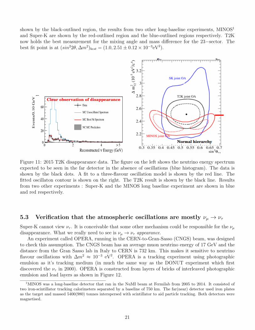
shown by the black-outlined region, the results from two other long-baseline experiments, MINOS1
and Super-K are shown by the red-outlined region and the blue-outlined regions respectively. T2Know holds the best measurement for the mixing angle and mass difference for the 23−sector. Thebest fit point is at (sin22θ,∆m2)best = (1.0, 2.51± 0.12× 10⁻³eV2).
Figure 11: 2015 T2K disappearance data. The figure on the left shows the neutrino energy spectrumexpected to be seen in the far detector in the absence of oscillations (blue histogram). The data isshown by the black dots. A fit to a three-flavour oscillation model is shown by the red line. Thefitted oscillaton contour is shown on the right. The T2K result is shown by the black line. Resultsfrom two other experiments : Super-K and the MINOS long baseline experiment are shown in blueand red respectively.
5.3 Verification that the atmospheric oscillations are mostly νµ → ντ
Super-K cannot view ντ . It is conceivable that some other mechanism could be responsible for the νµdisappearance. What we really need to see is νµ → ντ appearance.
An experiment called OPERA, running in the CERN-to-Gran-Sasso (CNGS) beam, was designedto check this assumption. The CNGS beam has an average muon neutrino energy of 17 GeV and thedistance from the Gran Sasso lab in Italy to CERN is 732 km. This makes it sensitive to neutrinoflavour oscillations with ∆m2 ≈ 10−3 eV2. OPERA is a tracking experiment using photographicemulsion as it’s tracking medium (in much the same way as the DONUT experiment which firstdiscovered the ντ in 2000). OPERA is constructed from layers of bricks of interleaved photographicemulsion and lead layers as shown in Figure 12.
1MINOS was a long-baseline detector that ran in the NuMI beam at Fermilab from 2005 to 2014. It consisted oftwo iron-scintillator tracking calorimeters separated by a baseline of 750 km. The far(near) detector used iron platesas the target and massed 5400(980) tonnes interspersed with scintillator to aid particle tracking. Both detectors weremagnetised.
21

Figure 12: (left) An OPERA brick containing layers of photographic emulsion and lead. (right)the measurement principle. Charged particles from interactions in the lead create short tracks inthe photographic emulsion which are measured in off-line scanners. A tau is recognised from thecharacteristic decay kink.
These bricks are replaceable and are arranged in two target walls separated by scintillator planes.The scintillator planes are used to localise the brick in which a neutrino interaction occurred. Oncethis vertex brick is known, it is removed from the detector and the photographic emulsion is developedand then scanned by sophisticated off-line image analysers. The interaction characteristics are thenmeasured. A charged-current interaction of a ντ generates a short τ track which typically decayshadronically. Figure 13 shows the first ντ interaction observed in a brick. The short yellow lines showthe track left by each particle as it moves through the photographic emulsion, and the connectinglines show the event reconstruction. The τ is the short red track near the vertex.
To date, OPERA has measured 5 ντ interaction with an expected background in the absenceof neutrino oscillations of 0.25 events. The oscillation analysis suggests a ∆m2 = 3.3 × 10⁻³ eV2,consistent with other oscillation experiments. From this we know that the atmospheric oscillationmode is mostly νµ → ντ .
5.4 What you should know
• How the atmospheric neutrino data can be interpreted in the context of two-flavour neutrinooscillations.
• What a long–baseline experiment is, and the difference between disappearance and appearanceexperiments.
• What the T2K experiment was and how it verified the atomspheric oscillation solution.
• You do not need to know the details of the OPERA experiment - just what it has been able toshow.
22
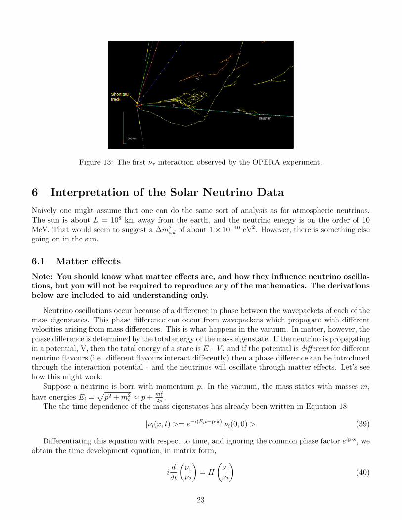
Figure 13: The first ντ interaction observed by the OPERA experiment.
6 Interpretation of the Solar Neutrino Data
Naively one might assume that one can do the same sort of analysis as for atmospheric neutrinos.The sun is about L = 108 km away from the earth, and the neutrino energy is on the order of 10MeV. That would seem to suggest a ∆m2
sol of about 1× 10⁻¹⁰ eV2. However, there is something elsegoing on in the sun.
6.1 Matter effects
Note: You should know what matter effects are, and how they influence neutrino oscilla-tions, but you will not be required to reproduce any of the mathematics. The derivationsbelow are included to aid understanding only.
Neutrino oscillations occur because of a difference in phase between the wavepackets of each of themass eigenstates. This phase difference can occur from wavepackets which propagate with differentvelocities arising from mass differences. This is what happens in the vacuum. In matter, however, thephase difference is determined by the total energy of the mass eigenstate. If the neutrino is propagatingin a potential, V, then the total energy of a state is E+V , and if the potential is different for differentneutrino flavours (i.e. different flavours interact differently) then a phase difference can be introducedthrough the interaction potential - and the neutrinos will oscillate through matter effects. Let’s seehow this might work.
Suppose a neutrino is born with momentum p. In the vacuum, the mass states with masses mi
have energies Ei =√p2 +m2
i ≈ p+m2i
2p.
The the time dependence of the mass eigenstates has already been written in Equation 18
|νi(x, t) >= e−i(Eit−p·x)|νi(0, 0) > (39)
Differentiating this equation with respect to time, and ignoring the common phase factor eip·x, weobtain the time development equation, in matrix form,
id
dt
(ν1
ν2
)= H
(ν1
ν2
)(40)
23

where H is the Hamiltonian operator. In a vacuum, this operator is
H =1
2E
(m2
1 00 m2
2
)(41)
Now, we can write Equation 40 in the flavour states, να and νβ, assuming the usual 2x2 mixingmatrix
U =
(cosθ sinθ−sinθ cosθ
)(42)
as (νανβ
)= U
(ν1
ν2
)(43)
Equation 40 may be expressed in the flavour basis as
id
dt
(ν1
ν2
)= U †i
d
dt
(νανβ
)= H
(ν1
ν2
)= HU †
(νανβ
)(44)
or, multiplying on the left by U
id
dt
(νανβ
)= UHU †
(νανβ
)(45)
In the vacuum, the transformed Hamiltonian is (trust me on this....)
Hf = UHU † =(m2
1 +m22)
2E1 +
∆m2
2E
(−cos2θ sin2θsin2θ cos2θ
)(46)
where 1 is the 2x2 unit matrix. For convenience, let’s label ((m2
1+m22
4E)1 as H0.
id
dt
(νανβ
)= [H0 +
∆m2
4E
(−cos2θ sin2θsin2θ cos2θ
)]
(νανβ
)(47)
Now, let’s suppose that the neutrinos are moving in a non-zero potential. Then you have to adda potential term to Schrodinger Equation
id
dt
(νανβ
)= (Hf + V )
(νανβ
)(48)
There is nothing to suggest that the interaction potential that να experiences is the same as thatwhich νβ experiences. Hence, labelling the potential that να experiences as Vα and the potential thatνβ experiences as Vβ then
id
dt
(νανβ
)= [H0 +
(−∆m2
4Ecos2θ + Vα
∆m2
4Esin2θ
∆m2
4Esin2θ ∆m2
4Ecos2θ + Vβ
)]
(νανβ
)(49)
Now, we can always add a constant to this without affecting the final result, because that constantwill eventually appear as a constant phase. When I take the modulus squared to get the probability,that constant phase will vanish. So, I’ll add a term proportional to −Vβ so Equation 49 becomes
id
dt
(νανβ
)= [H0 +
(−∆m2
4Ecos2θ + (Vα − Vβ) ∆m2
4Esin2θ
∆m2
4Esin2θ ∆m2
4Ecos2θ
)]
(νανβ
)2 (50)
2This means that only differences in potential matter, not absolute potential. As usual.
24

What does this mean? Well, compare Equation 49 and Equation 47. The addition of the interac-tion potential difference means that we can no longer say that(
νανβ
)=
(cosθ sinθ−sinθ cosθ
)(ν1
ν2
)(51)
The interaction has changed the mass eigenstates. You can get a picture of what is going on bythinking about throwing a cricket ball. In order to measure the mass of the ball, you can throw itwith a given force and measure how far it goes. If the ball is thrown with the same force in a viscousliquid, which simulates the interaction of the neutrino with its environment through the potential, itwill travel a shorter distance. If you couldn’t see the liquid, you would imagine that it had a heaviermass than its rest mass in vacuum - interaction with the environment gives the ball a heavier effectivemass. More rigorously, in a vacuum the neutrino mass eigenstate obeys the equation
E2 − p2 = m2i (52)
In a potential, V, this takes the form
(E + V )2 − p2 ≈ m2i + 2EV (53)
. The effective mass of the neutrino is now m′i =√m2i + 2EV So we need now to express Equation 50
in terms of mass eigenstates with mass eigenvalues equivalent to the effective masses, not the vacuummass values.
What potential are we talking about and why is there a difference between νe and νµ? Takingthe last part of that question first, we can see that there must be a difference in how the νe behavesin matter from how the νµ behaves in matter. Muon neutrinos produced in the solar core can onlyinteract via the neutral current. They don’t have enough energy to create a charged muon in thecharged current process. Electron neutrinos, however, can interact via both the charged and neutralcurrents. The Feynman diagrams are shown in Figure 14. Hence the electron neutrinos can interactdifferently from the other types of neutrinos. Although it won’t be important for our argument, thepotential difference we are concerned about has the form
Vα − Vβ = 2√
2GFENe (54)
where GF is the Fermi constant, E is the neutrino energy and Ne is the electron number density inmatter. This is sensible as (i) the cross section is a linear function of energy and (2) the more electronsthere are, the more charged current interactions the νe can have and the larger the difference betweenνe and νµ.
Transforming the flavour Hamiltonian back into the vacuum mass basis using the mixing matrix,U, we get
id
dt
(ν1
ν2
)= U †i
d
dt
(νανβ
)(55)
= U †[H0 +
(−∆m2
4Ecos2θ + (Vα − Vβ) ∆m2
4Esin2θ
∆m2
4Esin2θ ∆m2
4Ecos2θ
)]
(νανβ
)(56)
= (U †[H0 +
(−∆m2
4Ecos2θ ∆m2
4Esin2θ
∆m2
4Esin2θ ∆m2
4Ecos2θ
)]U + U †
(Vα − Vβ 0
0 0
)U ]
(ν1
ν2
)(57)
=1
2E[
(m2
1 00 m2
2
)+
(∆V cos2θ ∆V cosθsinθ
∆V cosθsinθ ∆V sin2θ
)]
(ν1
ν2
)(58)
= [1
2E
(m2
1 + ∆V cos2θ ∆V cosθsinθ∆V cosθsinθ m2
2 + ∆V sin2θ
)]
(ν1
ν2
)(59)
25
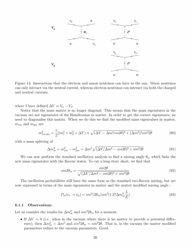
Figure 14: Interactions that the electron and muon neutrinos can have in the sun. Muon neutrinoscan only interact via the neutral current, whereas electron neutrinos can interact via both the chargedand neutral currents.
where I have defined ∆V ≡ Vα − Vβ.Notice that the mass matrix is no longer diagonal. This means that the mass eigenstates in the
vacuum are not eigenstates of the Hamiltonian in matter. In order to get the correct eigenstates, weneed to diagonalise this matrix. When we do this we find the modified mass eigenvalues in matter,m1m and m2m are
m21m,2m =
1
2[(m2
1 +m22 + ∆V )±
√(∆V −∆m2cos2θ)2 + (∆m2)2sin22θ (60)
with a mass splitting of
∆m2m = m2
1m −m22m = ∆m2
√(∆V/∆m2 − cos2θ)2 + sin22θ (61)
We can now perform the standard oscillation analysis to find a mixing angle θm which links thenew mass eigenstates with the flavour states. To cut a long story short, we find that
sin2θm =sin2θ√
(∆V /∆m2 − cos2θ)2 + sin22θ(62)
The oscillation probabilities still have the same form as the standard two-flavour mixing, but arenow expressed in terms of the mass eigenstates in matter and the matter modified mixing angle :
Pm(νe → νµ) = sin2(2θm)sin2(1.27∆m2m
L
E) (63)
6.1.1 Observations
Let us consider the results for ∆m2m and sin22θm for a moment.
• If ∆V = 0 (i.e. when in the vacuum where there is no matter to provide a potential differ-ence), then ∆m2
m = ∆m2 and sin22θm = sin22θ. That is, in the vacuum the matter modifiedparameters reduce to the vacuum parameters. Good.
26

• If sin22θ = 0, then sin22θm = 0, regardless of the potential. For there to be oscillations inmatter, one must already have the possibility of vacuum mixing.
• if the matter is very dense, ∆V → ∞, then sin22θm → 0. In very dense matter, oscillationscannot occur via matter effects or otherwise.
• if ∆V /∆m2 = cos2θ then the matter mixing angle is 1.0 - regardless of the value of the vacuummixing angle. This is interesting. Even if the vacuum mixing is tiny, there may still be somevalue of the electron number density where the probability of oscillations is 100%. This is calledthe MSW resonance.
• Notice that if ∆m2 → −∆m2 in Equation 62, the term (∆V /∆m2− cos2θ) in the denominatorwill have a different value and the effective mixing angle will be different. Using matter effectswe can obtain an estimate for the sign of the mass difference. Matter effects provide theonly means by which we can determine the sign of the mass difference - it cannotbe done with vacuum oscillations.
So what is going on in the sun? Well, suppose the electron neutrino is born in the solar core inconditions of high density. According to our results, it cannot oscillate there. It starts to propagateoutwards from the core, towards the vacuum. At some point, between the core and the vacuum, itcrosses a region of the sun with electron number density that fulfills the resonance condition. In thatregion it oscillates from νe to νµ. Once out of this region, the matter density is too small to supportmatter oscillations, and the νµ leaves the sun to travel to earth.
In other words, some solar neutrinos do not oscillate on their way from the edge of the sun toearth. They have already oscillated by the time they get to the outer regions of the sun. They aregenerated as νe and leave the sun as νµ.
I say “some” because the situation is furthur complicated by energy dependence. Some neutrinoshave so low an energy that they don’t oscillate in the sun, but do in the vacuum. If one plugs the solarparameters (below) into the two-flavour oscillation formula, one finds that the survival probabilityP (νe → νe) is about 57%. This explains the different fractions of νe observed by experiments withdifferent thresholds. At low energies, more neutrinos leave the sun without oscillating, but have a50% change of oscillating on the journey from sun to earth. As the energy increases, the probabilityof oscillation within the sun through the matter effect increases, so the survival probability decreases.We believe, incidentally, that matter enhanced oscillation predominantly affects the 7Be flux, butthe p-p flux should be minimally affected. More experiments capable of probing the very low energysolar flux, in order to check this, are being built and run as I write (see the Borexino experiment, forexample).
6.1.2 Solar Results
After analysis of all the solar data we find that it can be explained by the parameters
∆m2sol = (7.6± 0.2)× 10−5eV2 sin2(2θsol) = 0.8± 0.1 (64)
and that the oscillation is almost completely νe → νµ. It’s interesting to note that the solar mixingangle is not maximal - θ ≈ 32◦.
27

6.2 Verification of the solar oscillation parameters
In order to check the solar oscillation analysis we need to make an experiment which is sensitive to∆m2 ≈ 10−5 eV2. We can’t really do this with accelerators at the moment. The sort of energies onederives at accelerators is on the order of 1 GeV or larger, implying a baseline of L > 100000 km.That’s about 10 times the diameter of the planet.
Instead we make use of the other artifical terrestrial neutrino source - reactors. These produceelectron anti-neutrinos with energies around 5 MeV. Using these as a source, one only requires abaseline of about 100 km.
The experiment KamLAND is a liquid scintillator detector sited in the Kamioka mine next toSuper-Kamiokande in Japan. Japan has a thriving nuclear power industry, and at least 50 nuclearpower stations are close enough to Kamioka (see Figure 15) that KamLAND is capable of detectingνe from them. Since the energy of the antineutrinos is very low, KamLAND has to be extremelypure, else it will be overloaded by background from the radioactive decay of other isotopes in thelocal region or in the detector itself.
Figure 15: Locations of all nuclear reactors visible from the KamLAND detector.
KamLAND is a disappearance experiment. It has an advantage that the amount of matter be-tween the detector and the reactors is too small to support any type of MSW effect, so KamLANDshould measure the true solar vacuum oscillation parameters. Reactors produce pure beams of νe, soKamLAND trys to measure a deficit in the number of antineutrinos observed. Figure 16 shows thesolar oscillation parameter allowed region in the (sin2θ13,∆m
212) plane as measured by KamLAND
and by a compilation of the solar neutrino experiments. The best fit points for the solar oscillationparameters are (sin22θ12,∆m
212)best = (0.304+0.022
−0.016, 7.65+0.23−0.20 × 10⁻³ eV2). Notice, by the way, the
complementarity between KamLAND and the other solar experiments. The experiments viewing thesun have large statistical power, but poor energy resolution, leading to the vertical elliptical errorellipse in the allowed region. KamLAND, on the other hand, doesn’t see many events, but knows
28

what their energy is, so sets a more horizontal ellipse. The two constrain the allowed region to thesmall red region where both experiments are consistent.
Figure 16: Allowed region for the solar oscillation parameters. Here the best fit values are(sin22θ12,∆m
212)best = (0.304+0.022
−0.016, 7.65+0.23−0.20 × 10⁻³ eV2).
Figure 17 results shows a plot of the ratio of the observed to expected antineutrino events for anaverage L/E (an average since the neutrino sources are at different baselines - KamLAND just assignsall the events to an average L). This figure is the first actual proof that oscillations are happening - it’sthe first picture of an oscillation. KamLAND’s analysis, combined with the other solar experiments,yielded
∆m2sol = 7.9× 10⁻⁵eV2 sin2(2θsol) = 0.81 (65)
6.3 What you should know
• The general properties (both process and implications) of matter effects in neutrino oscillations(note : not the mathematics). One need only know that νe experiences interactions in matterthan the other flavours do not. This modifies the mixing angle and the mass squared differencefrom their vacuum values.
• How neutrino oscillations explain the solar results, and how this was confirmed using the Kam-LAND detector.
29

Figure 17: Ratio of observed to expected antineutrino rates as a function of the average L/E atKamLAND
7 Three Neutrino Oscillations
Of course, there are more than two neutrinos. There are three, and that implies that the mixingmatrix can be (i) 3x3 , (ii) complex and (iii) unitary. In this case we haveνeνµ
ντ
=
Ue1 Ue2 Ue3Uµ1 Uµ2 Uµ3
Uτ1 Uτ2 Uτ3
ν1
ν2
ν3
(66)
This is known as the Pontecorvo-Maka-Nakagawa-Sakata (PMNS) matrix and does the same job inthe neutrino sector as the CKM matrix does in the quark sector.
The fact that the matrix is unitary means that
U †U = I → U † = U−1 = (U∗)T (67)
and from this ν1
ν2
ν3
=
U∗e1 U∗µ1 U∗τ1
U∗e2 U∗µ2 U∗τ2
U∗e3 U∗µ3 U∗τ3
νeνµντ
(68)
The unitarity of the PMNS matrix gives several useful relations:Ue1 Ue2 Ue3Uµ1 Uµ2 Uµ3
Uτ1 Uτ2 Uτ3
U∗e1 U∗µ1 U∗τ1
U∗e2 U∗µ2 U∗τ2
U∗e3 U∗µ3 U∗τ3
=
1 0 00 1 00 0 1
(69)
30

so
Ue1U∗e1 + Uµ1U
∗µ1 + Uτ1U
∗τ1 = 1
Ue2U∗e2 + Uµ2U
∗µ2 + Uτ2U
∗τ2 = 1
Ue3U∗e3 + Uµ3U
∗µ3 + Uτ3U
∗τ3 = 1
Ue1U∗µ1 + Ue2U
∗µ2 + Ue3U
∗µ3 = 0
Ue1U∗τ1 + Ue2U
∗τ2 + Ue3U
∗τ3 = 0
Uµ1U∗τ1 + Uµ2U
∗τ2 + Uµ3U
∗τ3 = 0
(70)
The oscillation probability is calculated just as before. Assume that at time t=0, we create aneutrino in a pure |να > state.
|ψ(x = 0) >= Uα1|ν1 > +Uα2|ν2 > +Uα3|ν3 > (71)
The wavefunction evolves as
|ψ(t) >= Uα1|ν1 > e−ip1·x + Uα2|ν2 > e−ip2·x + Uα3|ν3 > e−ip3·x (72)
where pi · x = Eit − pi · x. After travelling a distance L the wavefunction is (assuming that theneutrino is relativistic)
|ψ(L) >= Uα1|ν1 > e−iφ1 + Uα2|ν2 > e−iφ2 + Uα3|ν3 > e−iφ3 (73)
with φi = pi · x = Eit− |pi|L ≈ (Ei − |pi|)L. As before, we can approximate Ei by
Ei ≈ pi +m2i
2Ei(74)
so
φi = (Ei − |pi|)L ≈m2i
2EiL (75)
.Expressing the mass eigenstates in terms of the flavour eigenstates:
|ψ(L) >=Uα1e−iφ1(U∗e1|νe > +U∗µ1|νµ > +U∗τ1|ντ >)
+ Uα2e−iφ2(U∗e2|νe > +U∗µ2|νµ > +U∗τ2|ντ >)
+ Uα3e−iφ3(U∗e3|νe > +U∗µ3|νµ > +U∗τ3|ντ >)
(76)
which can be arranged to give
|ψ(L) >=(Uα1U∗e1e−iφ1 + Uα2U
∗e2e−iφ2 + Uα3U
∗e3e−iφ3)|νe >
+ (Uα1U∗µ1e−iφ1 + Uα2U
∗µ2e−iφ2 + Uα3U
∗µ3e−iφ3)|νµ >
+ (Uα1U∗τ1e−iφ1 + Uα2U
∗τ2e−iφ2 + Uα3U
∗τ3e−iφ3)|ντ >
(77)
from which we can get the oscillation probability P (να → νβ) :
P (να → νβ) =| < νβ|ψ(L) > |2
= (Uα1U∗β1e−iφ1 + Uα2U
∗β2e−iφ2 + Uα3U
∗β3e−iφ3)2
(78)
31

Using the complex relationship
|z1 + z2 + z3|2 = |z1|2 + |z2|2 + |z3|2 + 2<(z1z∗2 + z1z
∗3 + z2z
∗3) (79)
we can write Equation 78 as (eventually - I will never ask you to do this derivation))
P (να → νβ) =δαβ − 4∑i>j
Re(U∗αiUβiUαjU∗βj)sin
2(∆m2ij
L
4E)
+ 2∑i>j
Im(U∗αiUβiUαjU∗βj)sin(∆m2
ij
L
2E)
(80)
The PMNS matrix is usually expressed by 3 rotation matrices and three complex phases:
U =
1 0 00 cosθ23 sinθ23
0 −sinθ23 cosθ23
cosθ13 0 sinθ13e−iδCP
0 1 0−sinθ13e
iδCP 0 cosθ13
cosθ12 sinθ12 0−sinθ12 cosθ12 0
0 0 1
1 0 00 eiβ 00 0 eiγ
(81)
The final sub-matrix in this expression include the so-called Majorana phases, eiβ and eiγ. This matrixplays no part in the description of neutrino flavour oscillations so we will ignore it for now. It does,however, play a part in neutrinoless double beta decay.
Ignoring the Majorana phases, we find that, when multplied out, the PMNS matrix is
U =
c12c13 s12c13 s13e−iδCP
−s12c23 − c12s23s13eiδCP c12c23 − s12s13s23e
iδCP c13s23
s12s23 − c12s13c23eiδCP −c12s23 − s12s13c23e
iδCP c13c23
(82)
where cij = cosθij and sij = sinθij. The first matrix is called the ”12-sector”, the second matrixis the ”13-sector”, and the third is the ”23-sector”. The second matrix is responsible, possibly, forCP-violation. We’ll talk about that below. For now let’s set δCP to zero. If this is the case, then theimaginary term in Equation 80 vanishes and we are left with
P (να → νβ) = δαβ − 4∑i>j
(UαiUβiUαjUβj)sin2(∆m2
ij
L
4E) (83)
We also must remember the squared mass difference. There are 3 neutrino mass eigenstates, andhence 2 independent mass splittings, called ∆m2
23 and ∆m212. The other splitting is defined by the
relationship∆m2
12 + ∆m223 + ∆m2
31 = 0 (84)
We know from the solar and atmospheric neutrino problems that these splittings have values around+8× 10⁻⁵ eV2 and 3× 10⁻³ eV2. To go ahead a bit, the mass splitting relating to the 23 sector isthe atmospheric neutrino mass difference : ∆m2
23 = 3× 10⁻³eV2 and the splitting relating to the 12sector is the solar mass difference : ∆m2
12 = 8× 10⁻⁵eV2
32

Let’s consider an appearance experiment. In this case α 6= β. Then
P (να → νβ) =− 4∑i>j
(UαiUβiUαjUβj)sin2(1.27∆m2
ij
L
E)
= −4[(Uα1Uβ1Uα2Uα2)sin2(1.27∆m212
L
E)
+ (Uα1Uβ1Uα3Uα3)sin2(1.27∆m213
L
E)
+ (Uα2Uβ2Uα3Uα3)sin2(1.27∆m223
L
E)]
(85)
Equation 85 can be split into two cases. The first occurs for experiments where L/E is small. Inthis case, ∆m2
12L/E is very small and
sin2(1.27∆m212
L
E)→ 0 (86)
So, with the reasonable approximation that ∆m213 ≈ ∆m2
23,
P (να → νβ) = −4[Uα1Uβ1Uα3Uβ3 + Uα2Uβ2Uα3Uβ3]sin2(1.27∆m223
L
E) (87)
The other case occurs when L/E is large. Then the terms involving ∆m223 and ∆m2
13 are rapidlyoscillating and average to 0.5
sin2(1.27∆m223
L
E)→< sin2(1.27∆m2
23
L
E) >=
1
2(88)
sin2(1.27∆m213
L
E)→< sin2(1.27∆m2
13
L
E) >=
1
2(89)
and
P (να → νβ) =− 4[(Uα1Uβ1Uα2Uβ2)sin2(1.27∆m212
L
E)
+1
2(Uα1Uβ1Uα3Uβ3 + Uα2Uβ2Uα3Uβ3)]
(90)
Replacing the elements Uij with the mixing angle terms from the PMNS matrix, and rememberingthat δCP = 0, we can use the unitarity relations in Equation set 70 to get (after a while) for the smallL/E case
P (νµ → ντ ) = cos4(θ13)sin2(2θ23)sin2(1.27∆m223
L
E) (91)
P (νe → νµ) = sin2(2θ13)sin2(θ23)sin2(1.27∆m223
L
E) (92)
P (νe → ντ ) = sin2(2θ13)cos2(θ23)sin2(1.27∆m223
L
E) (93)
and for the large L/E case
P (νe → νµ,τ ) = cos2(θ13)sin2(2θ12) sin2(1.27∆m212
L
E) +
1
2sin2(2θ13) (94)
Now, if θ13 = 0 then these equations reduce to:
33

• Small L/E :
P (νµ → ντ ) = sin2(2θ23)sin2(1.27∆m223
L
E)
P (νe → νµ) = 0
P (νe → ντ ) = 0
• Large L/E :
P (νe → νµ,τ ) = sin2(2θ12) sin2(1.27∆m212
L
E) (95)
These are the same equations we used for the atmospheric and solar oscillations. We thereforeidentify the 23-sector with atmospheric neutrinos with a ∆m2
23 ≈ 3 × 10⁻³ eV2, and the 12-sectorwith solar neutrinos with a ∆m2
12 ≈ 8× 10⁻⁵ eV2.We have some information about the atmospheric and solar oscillation sectors. We also know that
P (νµ → νe) is small for atmospheric neutrinos. This suggests that θ13 is small too. Can we do better?
7.1 How to measure θ13
We would like to be able to determine θ13 without having to include the other mixing angles. This isbecause, although measured, they have large errors, and inclusion will just make the θ13 measurementmore imprecise. We can do this by looking at the survival probability P (νe → νe). Going back toEquation 85, we can write
P (νe → νe) = 1− 4[U2e1U
2e2sin
2(1.27∆m212
L
E)
+ U2e1U
2e3sin
2(1.27∆m213
L
E)
+ U2e2U
2e3sin
2(1.27∆m223
L
E)]
(96)
Since ∆m213 ≈ ∆m2
23 and, from the unitarity conditions, U2e1 + U2
e2 + U2e3 = 1
P (νe → νe) = 1− 4[U2e1U
2e2sin
2(1.27∆m212
L
E) + U2
e3(1− U2e3)sin2(1.27∆m2
23
L
E)]
= 1− 4[(cosθ12cosθ13)2(sinθ12cosθ13)2sin2(1.27∆m212
L
E)
+ sin2(θ13)(1− sin2(θ13))sin2(1.27∆m223
L
E)]
= 1− cos4(θ13)(2sinθ12cosθ12)2sin2(1.27∆m212
L
E)
− (2cosθ13sinθ13)2sin2(1.27∆m223
L
E)
= 1− cos4θ13sin2(2θ12)sin2(1.27∆m2
12
L
E)− sin2(2θ13)sin2(1.27∆m2
23
L
E)
(97)
The first term has a contribution from the solar oscillation wavelength associated with the small masssplitting, ∆m2
12,
λsol = 2.47E
∆m212
, (98)
34

and the second term provides a contribution from the atmospheric oscillation wavelength associatedwith ∆m2
23,
λatm = 2.47E
∆m223
. (99)
For a 1 MeV neutrino, λsol = 33.0 km with ∆m212 = 7.5× 10⁻⁵ eV2, and λatm = 1.0 km with ∆m2
23 =2.4 × 10⁻³ eV2. At MeV energies, the solar-scale oscillations are far slower than the atmospheric-scale oscillations as shown in Figure 18 in which you can see the fast atmospheric-scale oscillationssuperimposed on the slower solar-scale oscillations3
Figure 18: The νe survival probability with θ13 = 15◦, ∆m212 = 7.5×10⁻⁵ eV2, ∆m2
23 = 2.4×10⁻³ eV2
and θ12 = 33◦. The fast oscillations, governed by the atmospheric mass scale, is superimposed on themuch slower solar-scale oscillation.
Close to the source, on a baseline of about a kilometre, we should only be sensitive to theatmospheric-scale oscillation term. The survival probability in this region is
P (νe → νe) ≈ 1− sin2(2θ13)sin2(1.27∆m223
L
E) (100)
which eliminates all the other mixing angles. So all we need to do is find a νe beam with energyaround a few MeV and put a detector at the right place, but on the scale of a kilometer of so fromthe source.
This is a bit difficult, however, as there are no known terrestrial νe sources which obey theseconditions. One has two possibilities : look for νe appearing in an a νµ beam or try to use the νegenerated in vast quantities in nuclear reactors. In order to use the latter source we must first find away to relate P (νe → νe) with P (νe → νe)?
7.1.1 C,P and T violation
Recall that there are three discrete symmetries used in particle physics:
• Charge conjugation C : C changes particles to antiparticles
3Just to be clear - the solar oscillation is not the average of the pattern shown in Figure 18. The probability functionis the sum of two different terms. The solar probability can be viewed as a line linking the top of the peaks in theoscillation pattern (so that the survival probability is 1.0 at zero distance). The atmospheric-scale oscillations subtractsa bit of survival probability from that baseline.
35
• Parity P : P reverses the spatial components of wavefunctions
• Time T : T reverses the interaction by running time backwards
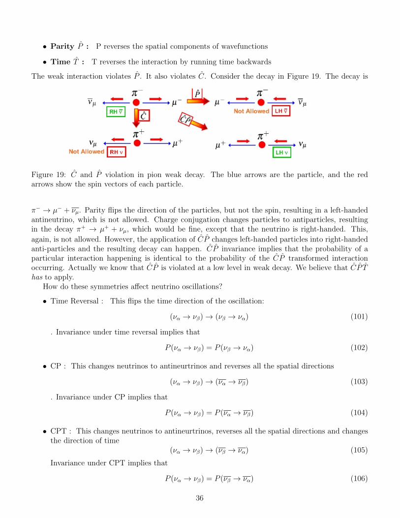
The weak interaction violates P . It also violates C. Consider the decay in Figure 19. The decay is
Figure 19: C and P violation in pion weak decay. The blue arrows are the particle, and the redarrows show the spin vectors of each particle.
π− → µ− + νµ. Parity flips the direction of the particles, but not the spin, resulting in a left-handedantineutrino, which is not allowed. Charge conjugation changes particles to antiparticles, resultingin the decay π+ → µ+ + νµ, which would be fine, except that the neutrino is right-handed. This,
again, is not allowed. However, the application of CP changes left-handed particles into right-handedanti-particles and the resulting decay can happen. CP invariance implies that the probability of aparticular interaction happening is identical to the probability of the CP transformed interactionoccurring. Actually we know that CP is violated at a low level in weak decay. We believe that CP Thas to apply.
How do these symmetries affect neutrino oscillations?
• Time Reversal : This flips the time direction of the oscillation:
(να → νβ)→ (νβ → να) (101)
. Invariance under time reversal implies that
P (να → νβ) = P (νβ → να) (102)
• CP : This changes neutrinos to antineurtrinos and reverses all the spatial directions
(να → νβ)→ (να → νβ) (103)
. Invariance under CP implies that
P (να → νβ) = P (να → νβ) (104)
• CPT : This changes neutrinos to antineurtrinos, reverses all the spatial directions and changesthe direction of time
(να → νβ)→ (νβ → να) (105)
Invariance under CPT implies that
P (να → νβ) = P (νβ → να) (106)
36

From the point of view of the νe experiment we were talking about above, CPT invariance impliesthat P (νe → νe) = P (νe → νe). Hence, the survival probability should be the same for electronantineutrinos from reactors as for electron neutrinos of the same energies :
P (νe → νe) = 1− sin2(2θ13)sin2(1.27∆m223
L
E) = P (νe → νe) (107)
7.2 The measurement of θ13
A good way, then, of measuring θ13 is to look at the disappearance of νe in a flux of neutrinos froma reactor. The detector should be placed about 1 km away so there is no interference from the solaroscillation term. This was finally done in 2012 by three reactor experiments : Daya Bay in China,Double CHOOZ in France and RENO in South Korea. Of interest to this story is Daya Bay - areactor experiment with the largest reach in measuring θ13. Daya Bay is in Southern China, nearHong Kong. It comprises 6 nuclear reactor cores, providing a hugh flux of electron anti-neutrinos.The cores are viewed by six 20 ton liquid scintillator detectors at baselines of 360 m, 500 m and1700 m from the reactors as shown in Figure 20 The addition of these medium baseline detectors arevaluable in measuring the L/E behaviour of any oscillation observed.
Figure 20: (left) A schematic of the Daya Bay experiment, showing the six reactor cores used togenerate the νe flux and the location of the 6 detectors at different baselines (right) Daya Bay’sreported results. The histogram shows the energy spectrum of νe expected in the absence of oscillations(blue histogram) and the measured energy spectrum (black dots).
In 2012 Daya Bay reported a positive measurement of sin2(2θ13). This is shown on the right ofFigure 20. The histogram shows the measured energy spectrum of νe from the reactors in the absenceof oscillations. The data points show the measurements. There is a clear deficit in the observed dataat the peak. Futhermore, the deficit is baseline-dependent. If interpreted as arising from neutrinooscillations, this deficit can be used to measure θ13. The result is sin2(2θ13) = 0.085 ± 0.006. Thisgives a mixing angle of θ13 ≈ 8.6◦. This result was quickly validated by measurements from RENO
37

and Double CHOOZ who reported mixing angle measurements of sin2(2θ13) = 0.113 ± 0.02 andsin2(2θ13) = 0.107± 0.05. It seems that θ13 is actually quite large.
7.2.1 T2K Returns
T2K was mentioned above in the context of the measurement of ∆m223 and sin2(2θ23) using νµ disap-
pearance. However, it was designed and built primarily to measure θ13 by looking for νe appearancein a νµ beam. The oscillation probability has been calculated above and is, in the two-flavour approx-imation,
P (νµ → νe) = sin2(2θ13)sin2(θ23)sin2(1.27∆m223
L
E) (108)
The T2K beam is almost pure νµ so the idea is to look for the appearance of electron-type neutrinosin the far detector, Super-Kamiokande. T2K uses the electron identification properties of the Super-Kamiokande detector.
Figure 21: The 68as a function of δCP assuming normal hierarchy (top) and inverted hierarchy(bottom). The solid line represents the best fit sin2(2θ13) value for the given δCP values. The shadedregion shows the average θ13 from reactor experiments world-wide.
T2K switched on in mid-2010. In March 2011 it was hit by the Japanese earthquake and onlystarted to taking data again a year later, in March 2012. It took neutrino-mode data until 2015, atwhich point it swapped the polarity of the beam and is now taking antineutrino data. In the electronneutrino apeearance search, the far detector recorded 28 electron neutrino interactions associatedwith the T2K beam. It expected to see 11 events from known background sources. The discrepancyrepresents a 7 σ positive result. The 68% and 90% confidence region for sin2(2θ13) as a function of δCP
38

are shown in Figure 21. Normal hierarchy is shown on the top plot and inverted hierarchy is shown onthe bottom plot. The shaded region shows the average θ13 result from the reactor experiments. Boththe reactor experiments and T2K are consistent. One could argue that T2K data favours a δCP < 0(although not with any great statistical justification).
The global average of all θ13 results is
sin2(2θ13) = 0.094+0.007−0.009 (109)
7.3 What you need to know
• How, and under what conditions, the three flavour neutrino oscillation probability splits intothe “atmospheric” and the “solar” sectors.
• The importance of θ13 and the methods used to measure it. You don’t need to know great detail- just the oscillations modes that are used to make the measurement and the result.
8 Summary of Current Knowledge and open questions
We can now summarise our current level of knowledge of neutrino oscillations and neutrino mass fromoscillation experiments.
We now know that there are 3 light neutrinos. The neutrino mass states are different from theflavour states. There are two mass splittings
∆m212 = +7.54× 10⁻⁵eV2 (110)
and|∆m2
23| = 2.4× 10⁻³eV2 (111)
We know the sign of ∆m212 but not ∆m2
23. This is shown in Figure 22. The mixing angles have now
Figure 22: Current knowledge of neutrino mass eigenstate splitting (assuming θ13 is zero).
all been determined, to various levels of precision, and are shown in Table 2
8.1 Open Questions
There are a number of questions currently left open:
• We need to obtain better estimates of sin2(2θ23),∆m223, sin
2(2θ12) and ∆m212.
39

• Is θ23 = 45 degrees or not?
• Is the mass hierarchy normal (∆m223 > 0) or inverted (∆m2
23 < 0)?
• Are the neutrinos and antineutrinos identical? This cannot be answered by an oscillation ex-periment.
• What is the absolute neutrino mass? This cannot be measured by an oscillation experiments.
• Why is the MNSP matrix so different in form to the CKM matrix? This will require a deeperunderstanding of flavour and mass generation mechanisms.
• What is the value of δCP ?
The final question is the ultimate measurement we wish to make in neutrino physics and informsthe future 20-25 years of the field.
8.2 What you should know
• The identify of each sub–matrix of the PMNS matrix. What do each of the correspond to, interms of oscillations and what are the measured values of each of the mixing angles.
• The general state of parameter measurements (I won’t expect detailed numbers but you shouldknow the values of the mixing angles to the degree or so).
• What are the current open questions in neutrino physics?
9 A Spanner In The Works?
To date we have built up a nice coherent theory of 3-flavour neutrino oscillations that seems to besupported by the available data. I am now going to throw a handful of spanners into the machinery.These may be very heavy-duty spanners, which have the potential to stomp this nice framework intokindling (to recklessly mix my metaphors), or they may be light-weight chocolate spanners whichwon’t survive being exposed to the sunlight of extra data (metaphor. mix.) - we don’t know yet. Thefirst spanner is called LSND.
9.1 LSND
The LSND detector (Liquid Scintillator Neutrino Detector) was the first oscillation experiment toreport a positive result. It was an experiment designed to search for νµ → νe oscillations through theappearance of a νe in the single near detector.
Parameter Measurement Anglesin2(2θ23) > 0.92 (45.0± 2.4)◦
sin2(2θ12) 0.85± 0.03 (33.6± 0.8)◦
sin2(2θ13) 0.084± 0.01 (8.9± 0.3)◦
Table 2: Current results of measurements of all mixing angles in the PMNS matrix.
40
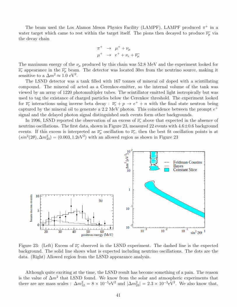
The beam used the Los Alamos Meson Physics Facility (LAMPF). LAMPF produced π+ in awater target which came to rest within the target itself. The pions then decayed to produce νµ viathe decay chain
π+ → µ+ + νµ
µ+ → e+ + νe + νµ
The maximum energy of the νµ produced by this chain was 52.8 MeV and the experiment looked forνe appearance in the νµ beam. The detector was located 30m from the neutrino source, making itsensitive to a ∆m2 ≈ 1.0 eV2.
The LSND detector was a tank filled with 167 tonnes of mineral oil doped with a scintillatingcompound. The mineral oil acted as a Cerenkov-emitter, so the internal volume of the tank wasviewed by an array of 1220 photomultipler tubes. The scintillator emitted light isotropically but wasused to tag the existance of charged particles below the Cerenkov threshold. The experiment lookedfor νe interactions using inverse beta decay : νe + p → e+ + n with the final state neutron beingcaptured by the mineral oil to generate a 2.2 MeV photon. This coincidence between the prompt e+
signal and the delayed photon signal distinguished such events form other backgrounds.In 1996, LSND reported the observation of an excess of νe above that expected in the absence of
neutrino oscillations. The first data, shown in Figure 23, measured 22 events with 4.6±0.6 backgroundevents. If this excess is interpreted as νµ oscillation to νe, then the best fit oscillation points is at(sin2(2θ),∆m2
23) = (0.003, 1.2eV2) with an allowed region as shown in Figure 23
Figure 23: (Left) Excess of νe observed in the LSND experiment. The dashed line is the expectedbackground. The solid line shows what is expected including neutrino oscillations. The dots are thedata. (Right) Allowed region from the LSND appearance analysis.
Although quite exciting at the time, the LSND result has become something of a pain. The reasonis the value of ∆m2 that LSND found. We know from the solar and atmospheric experiments thatthere are are mass scales : ∆m2
12 = 8 × 10⁻⁵eV2 and |∆m223| = 2.3 × 10⁻³eV2. We also know that,
41
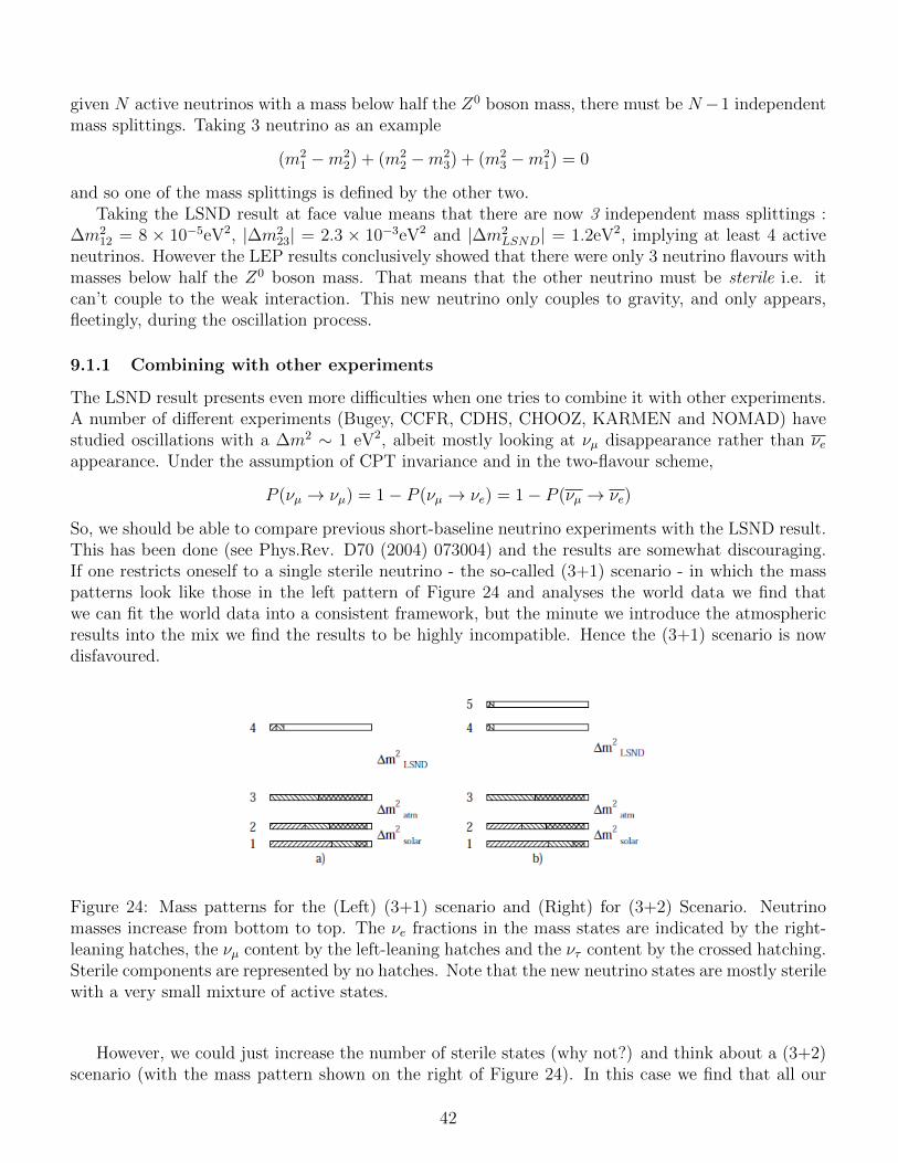
given N active neutrinos with a mass below half the Z0 boson mass, there must be N−1 independentmass splittings. Taking 3 neutrino as an example
(m21 −m2
2) + (m22 −m2
3) + (m23 −m2
1) = 0
and so one of the mass splittings is defined by the other two.Taking the LSND result at face value means that there are now 3 independent mass splittings :
∆m212 = 8 × 10⁻⁵eV2, |∆m2
23| = 2.3 × 10⁻³eV2 and |∆m2LSND| = 1.2eV2, implying at least 4 active
neutrinos. However the LEP results conclusively showed that there were only 3 neutrino flavours withmasses below half the Z0 boson mass. That means that the other neutrino must be sterile i.e. itcan’t couple to the weak interaction. This new neutrino only couples to gravity, and only appears,fleetingly, during the oscillation process.
9.1.1 Combining with other experiments
The LSND result presents even more difficulties when one tries to combine it with other experiments.A number of different experiments (Bugey, CCFR, CDHS, CHOOZ, KARMEN and NOMAD) havestudied oscillations with a ∆m2 ∼ 1 eV2, albeit mostly looking at νµ disappearance rather than νeappearance. Under the assumption of CPT invariance and in the two-flavour scheme,
P (νµ → νµ) = 1− P (νµ → νe) = 1− P (νµ → νe)
So, we should be able to compare previous short-baseline neutrino experiments with the LSND result.This has been done (see Phys.Rev. D70 (2004) 073004) and the results are somewhat discouraging.If one restricts oneself to a single sterile neutrino - the so-called (3+1) scenario - in which the masspatterns look like those in the left pattern of Figure 24 and analyses the world data we find thatwe can fit the world data into a consistent framework, but the minute we introduce the atmosphericresults into the mix we find the results to be highly incompatible. Hence the (3+1) scenario is nowdisfavoured.
Figure 24: Mass patterns for the (Left) (3+1) scenario and (Right) for (3+2) Scenario. Neutrinomasses increase from bottom to top. The νe fractions in the mass states are indicated by the right-leaning hatches, the νµ content by the left-leaning hatches and the ντ content by the crossed hatching.Sterile components are represented by no hatches. Note that the new neutrino states are mostly sterilewith a very small mixture of active states.
However, we could just increase the number of sterile states (why not?) and think about a (3+2)scenario (with the mass pattern shown on the right of Figure 24). In this case we find that all our
42
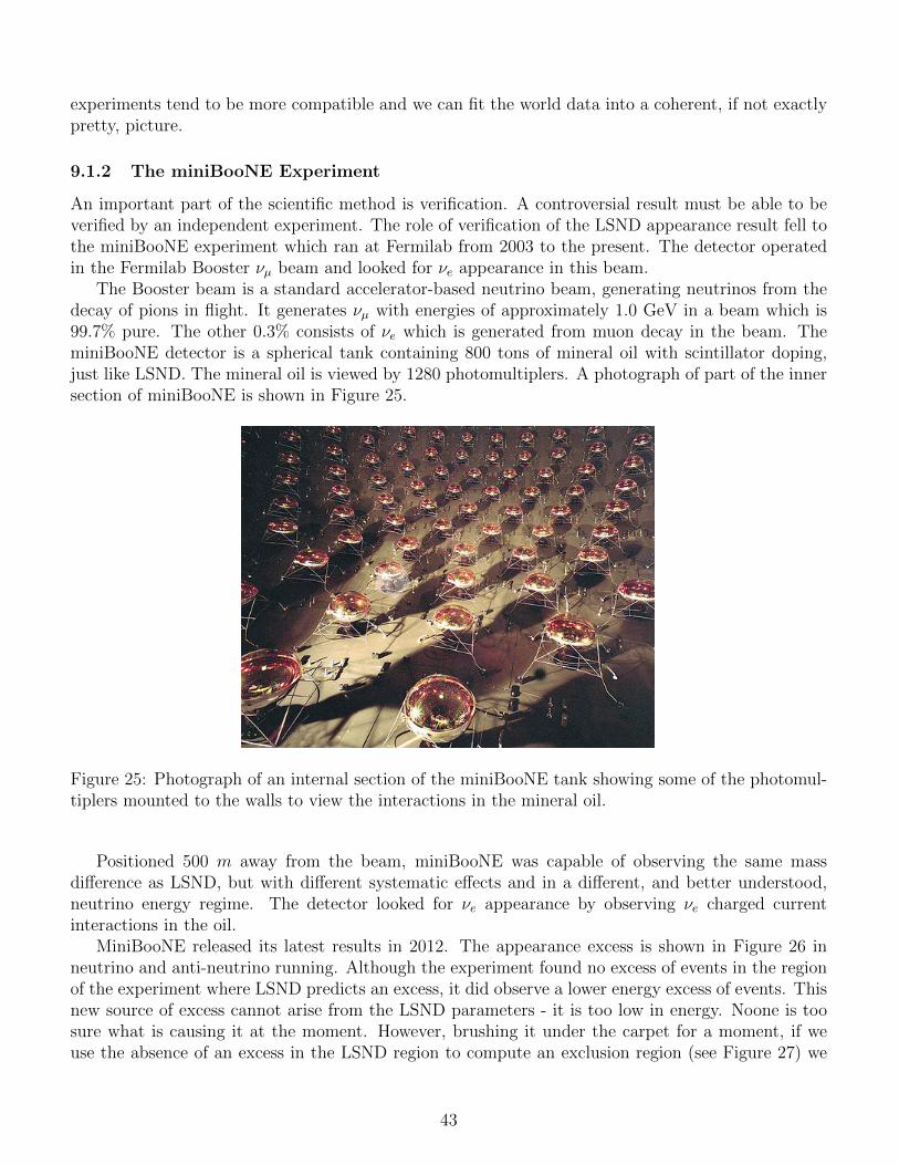
experiments tend to be more compatible and we can fit the world data into a coherent, if not exactlypretty, picture.
9.1.2 The miniBooNE Experiment
An important part of the scientific method is verification. A controversial result must be able to beverified by an independent experiment. The role of verification of the LSND appearance result fell tothe miniBooNE experiment which ran at Fermilab from 2003 to the present. The detector operatedin the Fermilab Booster νµ beam and looked for νe appearance in this beam.
The Booster beam is a standard accelerator-based neutrino beam, generating neutrinos from thedecay of pions in flight. It generates νµ with energies of approximately 1.0 GeV in a beam which is99.7% pure. The other 0.3% consists of νe which is generated from muon decay in the beam. TheminiBooNE detector is a spherical tank containing 800 tons of mineral oil with scintillator doping,just like LSND. The mineral oil is viewed by 1280 photomultiplers. A photograph of part of the innersection of miniBooNE is shown in Figure 25.
Figure 25: Photograph of an internal section of the miniBooNE tank showing some of the photomul-tiplers mounted to the walls to view the interactions in the mineral oil.
Positioned 500 m away from the beam, miniBooNE was capable of observing the same massdifference as LSND, but with different systematic effects and in a different, and better understood,neutrino energy regime. The detector looked for νe appearance by observing νe charged currentinteractions in the oil.
MiniBooNE released its latest results in 2012. The appearance excess is shown in Figure 26 inneutrino and anti-neutrino running. Although the experiment found no excess of events in the regionof the experiment where LSND predicts an excess, it did observe a lower energy excess of events. Thisnew source of excess cannot arise from the LSND parameters - it is too low in energy. Noone is toosure what is causing it at the moment. However, brushing it under the carpet for a moment, if weuse the absence of an excess in the LSND region to compute an exclusion region (see Figure 27) we
43

find that miniBooNE rules out a large fraction of the LSND allowed region, but not, unfortunately,all of it.
Figure 26: Excess of (left) νe and (right) νe events observed in the miniBooNE experiment. The dotsshow the data. The coloured histograms show the expected background from a number of differentbackground sources. Both neutrino and antineutrino data show an excess of events at low energy.
One of the main criticisms of the miniBooNE experiment has always been that it is searching forνµ → νe oscillations whereas LSND was measuring νµ → νe oscillations. Although CPT symmetriesstate that the two should have the same probabilities, this sort of loop-hole worries experimentalists.In 2009, the Booster neutrino beam switched to running antineutrinos so that a direct comparisonbetween miniBooNE and LSND could be made. The results are shown in Figure 26. As with theneutrino data, an excess at lower energies is observed (making it more likely to be a result of someunknown background source than oscillations in my humble opinion).
So where are we left with the LSND problem? Unfortunately not much further. We still have anexcess in the LSND data, but there is now also a different excess in the miniBoone data. None ofthis is easy to interpret so the only conclusion we can really make is that we need more data to workout what is going on. The best model that even vaguely fits the data is a (3+2) sterile scenario withlarge CP violation, but this is all beyond-Standard Model physics.
9.2 The Reactor and Gallium Anomalies
Two other anomalies which may be suggestive of the existance of at least one sterile neutrino havealso recently floated into view. The reactor anomaly arose after the introduction of new and verydetailed calculations of the νe flux from reactors in 2011. Up to that point the prediction of νe eventrates in reactor experiments very close to the reactor core agreed reasonably well. However, the newflux was approximately 4% larger than earlier calculations. Were this to be correct, it would implythat the reactor data actually displayed a disappearance of νe by the same 4%. Were this “missingflux” to be attributed to νe oscillating to some sterile state, it would have to an oscillation modewith ∆m2 ≈ 1 eV2. It should be noted that calculating the reactor flux in detail is a very complexproblem so it may be that there is still some error in the new calculations. The other anomaly is theso-called Gallium anomaly. Here the gallium radiochemical experiments, SAGE and GALLEX, wereengaged in some radioactive calibration using a large source of νe. Again, their observed rates were
44

Figure 27: The region of the parameter space excluded by the miniBooNE results. The LSND regionis only partially ruled out.
lower than expected given the source activity and, again, this could be interpreted as arising fromneutrinos oscillating to some sterile state with ∆m2 ≈ 1 eV2. Both of these anomalies exist at the2σ level so it would be wise to view them with some scepticism at the moment. 2-3 σ discrepanciesappear, and disappear, with alarming regularity in science.
9.3 What you should know
• What LSND was, what its main result was and what that would imply about neutrinos.
• What the miniBooNE experiment found.
• Brief details of the reactor and Gallium anomalies.
I won’t ask for specifics but you should know why these results are controversial.Now let’s brush the whole sterile neutrino issue under a very large carpet and talk about
10 The Future
The measurement of θ13 has been a decision point in what neutrino physics does in the future. Sinceθ13 is quite large and accessible, we now want to make precision measurements of the mixing angles.We are left with two parameters to measure : the mass hierarchy and δCP . We expect the masshierarchy can be measured in next generation experiments within the next decade or so. The CPviolating parameter is a harder measurements and will take a little longer.
45
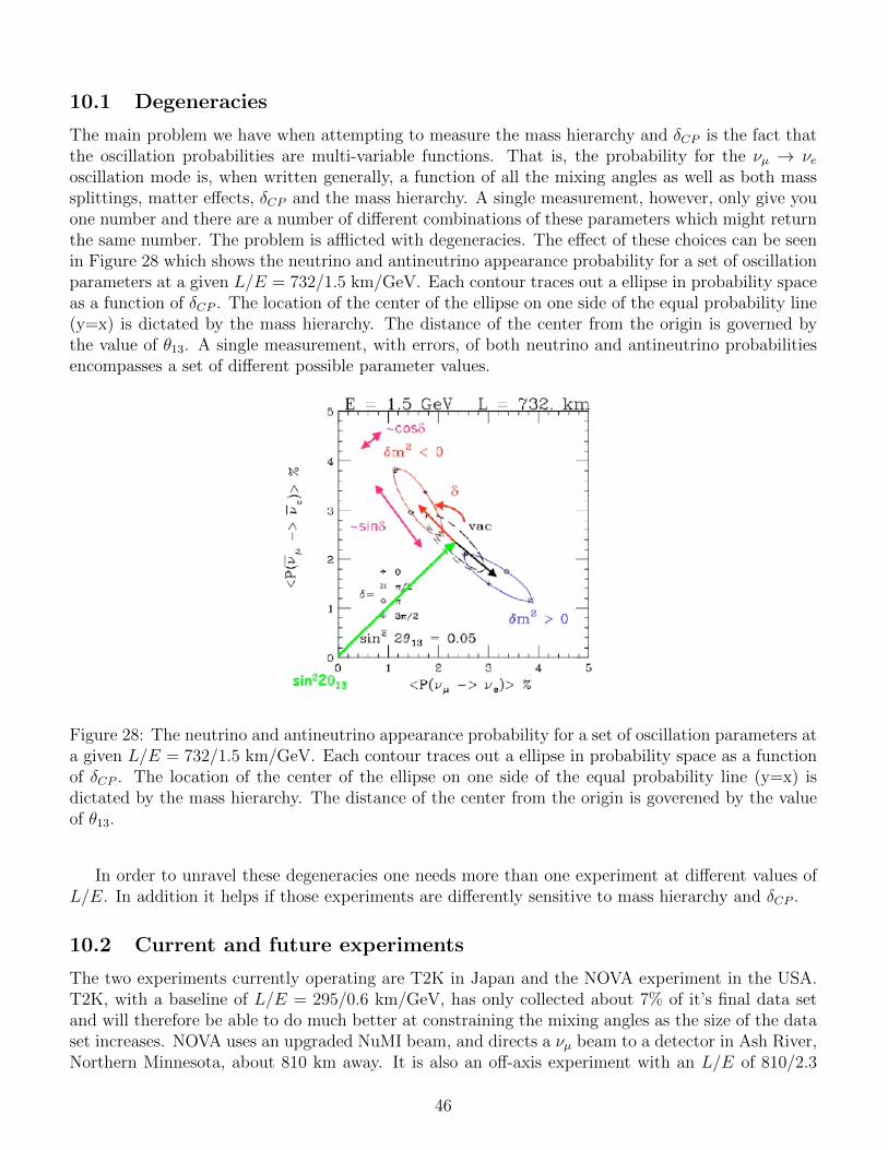
10.1 Degeneracies
The main problem we have when attempting to measure the mass hierarchy and δCP is the fact thatthe oscillation probabilities are multi-variable functions. That is, the probability for the νµ → νeoscillation mode is, when written generally, a function of all the mixing angles as well as both masssplittings, matter effects, δCP and the mass hierarchy. A single measurement, however, only give youone number and there are a number of different combinations of these parameters which might returnthe same number. The problem is afflicted with degeneracies. The effect of these choices can be seenin Figure 28 which shows the neutrino and antineutrino appearance probability for a set of oscillationparameters at a given L/E = 732/1.5 km/GeV. Each contour traces out a ellipse in probability spaceas a function of δCP . The location of the center of the ellipse on one side of the equal probability line(y=x) is dictated by the mass hierarchy. The distance of the center from the origin is governed bythe value of θ13. A single measurement, with errors, of both neutrino and antineutrino probabilitiesencompasses a set of different possible parameter values.
Figure 28: The neutrino and antineutrino appearance probability for a set of oscillation parameters ata given L/E = 732/1.5 km/GeV. Each contour traces out a ellipse in probability space as a functionof δCP . The location of the center of the ellipse on one side of the equal probability line (y=x) isdictated by the mass hierarchy. The distance of the center from the origin is goverened by the valueof θ13.
In order to unravel these degeneracies one needs more than one experiment at different values ofL/E. In addition it helps if those experiments are differently sensitive to mass hierarchy and δCP .
10.2 Current and future experiments
The two experiments currently operating are T2K in Japan and the NOVA experiment in the USA.T2K, with a baseline of L/E = 295/0.6 km/GeV, has only collected about 7% of it’s final data setand will therefore be able to do much better at constraining the mixing angles as the size of the dataset increases. NOVA uses an upgraded NuMI beam, and directs a νµ beam to a detector in Ash River,Northern Minnesota, about 810 km away. It is also an off-axis experiment with an L/E of 810/2.3
46

km/GeV. Since the far detector is further away than it is in T2K, NOVA is sensitive to effects fromthe matter in the earth between source and detector, just like the solar experiments. Hence, NOVAcan also potentially measure the mass hierarchy in the 23-sector (remember that we know |∆m2
23| butnot the absolute value). NOVA is starting to produce results now.
The next generation of long baseline experiments are now being designed. The first is Hyper-Kamiokande, a direct upgrade of T2K. Hyper-K still used the water Cerenkov techniques but upgradesthe T2K beam to 750 kW and increases the size of the far detector to about half a megaton of water.Hyper-K has the same L/E as T2K. The second experiment is DUNE, which directs an upgradedneutrino beam with an average energy of 3 GeV from Fermilab to a set of large liquid argon TPCdetectors 1300 km away in the Homestake mine in South Dakota. For good physics reasons discussedbelow, DUNE utilises a wide-band, rather than off-axis, beam. The mass of the far detector is only70 kton (not 500, as in Hyper-K) but this is compensated for by a far more powerful beam (1.2 MW)and more precise detectors. Both experiments are currently in the design and proto-typing phasewith the expectation of turning on around 2025 or so.
10.3 Mass hierarchy measurements
The mass hierarchy can be estimate in one of two ways : comparison of the results of two experimentsmaking νµ → νe and νµ → νe appearance measurements at different baselines, or by using neutrinolessdouble beta decay. The current experiments (T2K and NOVA) can do this if they run for about 5years in neutrino and an equal event rate for antineutrinos. Figure 29 shows that combining T2K andNOVA data we have the potential to determine the mass hierarchy to 2-3 σ over a limited range ofδCP . This can be done in the next 5 years or so.
Figure 29: Sensitivity to the mass hierarchy as a function of δCP if we combine NOVA and T2K data.The plot shows that, with 6 years of NOVA running (3 neutrino and 3 antineutrino) combined withthe same for T2K running, we have the potential to determine the mass hierarchy to 2.0 or 3.0 σ overa limited range of δCP .
If we make the same plot for the next generation of experiments - here we use DUNE - as in Figure30 we see that the mass hierarchy can be determined to 5 σ over the entire range of δCP after about4 years or running. Of course, we need to build DUNE first so this result wouldn’t be ready until atleast 2025.
47

Figure 30: Sensitivity to the mass hierarchy using just the DUNE experiment running for 4 years.The mass hierarchy could be determined to better than 5 σ over the entire range of δCP .
An alternate way to determine the mass hierarchy is with neutrinoless double beta decay. Theinteraction rate for this process is proportional to the electron neutrino mass, and hence is proportionalto the linear combination of mass states. That is,
Γ0νββ ∝ mνe =3∑i=1
|Uei|2mi =3∑i=1
|Uei|2√
∆m2i3 +m2
3
In the inverted hierarchy, m3 � m1 ≈ m2 and ∆m213 ≈ ∆m2
23, so we can write
mνe = |Ue1|2√
∆m223 +m2
3 + |Ue2|2√
∆m223 +m2
3 + |Ue3|2m3
Since the lightest mass state, m3 > 0, we have
mνe > (|Ue1|2 + |Ue2|2)√
∆m223
= (1− |Ue3|2)√
∆m223
= cos2θ13
√∆m2
23
where the second last step comes from the fact that the PMNS matrix is unitary. The conclusion isthat, if the hierarchy is inverted, the electron neutrino mass mνe must have a lower bound. Figure31 shows the behaviour of the electron neutrino mas, mνe as a function of the lightest mass statefor the normal and inverted hierarchy. The bands show the spread in mνe from different guessesof the Majorana phases in the PMNS matrix (remember the ones we dropped when talking aboutoscillations?). The behaviour is quite complicated, but the thing to focus on is that, in the case ofthe inverted hierarchy and at low m3, mνe > 0.01 eV. Hence, if the current or next generation of
48

neutrinoless double beta decay experiments were able to put a limit on the electron neutrino mass ofless than 0.01 eV they would be able to rule out the inverted hierarchy. The current experimentallimits are an order of magnitude larger so there is work to do - we need larger experiments and longerrunning time. Of course, this is all predicated on the assumption that the neutrino is a Majoranaparticle. If it isn’t then cannot make this conclusion (we’ll never see anything, but that’s becausethere’s nothing to see...).
Figure 31: Dependence of the electron neutrino mass, mνe , on the lightest mass state for the neutri-noless double beta decay process.
In general we expect that we will know the mass hierarchy by about 2025 or so, with goodindications within the next 5 years.
10.4 Measuring δCP
For reasons we’ve already discussed (see-saw, leptogenesis, etc) determining if there is CP-violation inthe lepton sector is the major goal of the world-wide neutrino programme. Once the mass hierarchyis determined, measurement of δCP becomes fairly straight forward. Since δCP only appears as acomplex parameter in the PMNS matrix, it can only be accessed by measurements sensitive to thecomplex nature of the matrix. The flavour change probability is
P (να → νβ) = δαβ − 4∑i>j
<(U∗αiUβiUαjU∗βi)sin
2(∆m2ij
L
4E) + 2
∑i>j
=(U∗αiUβiUαjU∗βi)sin(∆m2
ij
L
4E)
(112)If we are performing a disappearance experiment, then α = β, and =(U∗αiUβiUαjU
∗βi) = 0. Hence, any
experiment that wants to be sensitive to δCP has to be an appearance experiment.There are two ways to measure δCP once the mass hierarchy is known:
1. Measure the flavour change probabilities for νµ → νe and νµ → νe. As shown in Figure 28, oncethese probabilities are known sufficiently precisely one can localise δCP on the ellipse. Hyper-K,which has the use of an off-axis beam, will try to use this method. Figure 32 shows the expectedsensitivity of HyperK to δCP as a function of δCP . The plot shows that HyperK believes it canstate that δCP is non-zero at 5(3)σ if 40(20)◦ < |δCP | < 140(160)◦. Doing so, however, requires
49

us to make precise measurements of the anti-neutrino flavour change probability. In general,with accelerator beams, the flux of antineutrinos tends to be lower than that of neutrinos.Combine this with a cross section for anti-neutrino interacting on a nucleus of only half to athird of neutrino cross section and the observed anti-neutrino event rate can be a factor of 4 or6 lower than the corresponding neutrino event rate. For the same statistical power, one wouldhave to run in anti-neutrino mode 4 to 6 times longer than the neutrino mode which has cashand scheduling implications (do you have grant for running that long? Will the acceleratorcomplex allow you to do so, etc etc).
Figure 32: Sensitivity of Hyper-K to non-zero δCP . The vertical axis measures the zero-δCP exclusionerror.
2. The other method is more subtle but allows you to measure δCP only using neutrino oscillations,hence speeding up the measurement. The left hand plot in Figure 33 plots the appearanceprobability, P (νµ → νe), as a function of neutrino energy for the DUNE baseline length of 1300km between source and detector and for different assumed values of δCP . You can see all the ofthe θ13 oscillation peaks superimposed on top of the solar oscillation line. The important pointto note is the difference in size between the first (at a neutrino energy of around 2 GeV) and thesecond (at around 0.8 GeV) oscillation peaks as a function of δCP . When δCP is zero, the twopeaks have roughly the sample value. However, if δCP is ±π
2the first or second peak are larger.
Hence, if the experiment is capable of resolving the two peaks one can measure δCP withoutrequiring antineutrinos. This is what DUNE, which has been designed with a wide-band beam,is designed to do. DUNE’s sensitivity to non-zero δCP can be seen on the right-hand plot ofFigure 33. It is quite similar to that from Hyper-K, although may be achieved faster with thewide-band beam.
So, is there any indication of a non-zero δCP . Actually yes there is. This comes from an analysisby T2K. Figure 34 shows the change in fit χ2 of a full 3-flavour model with possible non-zero δCP toa combination of T2K and reactor data. The black and red lines are the normal and inverted massheirarchies respectively. Ignore the blue lines. What this plot shows is that a better fit is achieved ifδCP is around −π
2. That is, there are indications that in order to best fit an oscillation model to the
T2K and reactor data, δCP must be non-zero.This is suggestive, but hardly conclusive. However it does mean that we neutrino experimentalists
have something to look forward to as the region of δCP suggested by T2K and the reactor data isprecisely where DUNE and HyperK are most sensitive. We probably will know if δCP is large by2025-2030.
50

Figure 33: (Left) The appearance probability, P (νµ → νe), as a function of neutrino energy for theDUNE baseline length of 1300 km between source and detector and for different assumed values ofδCP (from DUNE CDR Volume 2). (Right) Sensitivity to non-zero δCP .
10.5 What you need to know
• Why measuring the mass hierarchy and δCP is difficult (degeneracies)
• How mass hierarchy and δCP measurements are done.
• The experiments are planned to measure these. Detailed knowledge of experimental sensitivitiesis not necessary.
51

Figure 34: Change in fit χ2 from minimum χ2 from a fit of an oscillation model to the T2K andreactor data.
52