NNeeaarr--tthhrreesshhoolldd ffaattiigguuee ccrraacckk ggrroowwtthh bbeehhaavviioouurr ooff mmiilldd sstteeeell iinn sstteeaamm dduurriinngg rroottaattiinngg bbeennddiinngg

by

Ulyate Andries Curle

Submitted in partial fulfilment of the requirements for the degree

Master of Engineering

(Metallurgical Engineering)

in the

Faculty of Engineering, Build Environment and Information

Technology

University of Pretoria

Pretoria

November 2006

Department of Materials Science and Metallurgical Engineering

University of Pretoria

ii

Near-threshold fatigue crack growth behaviour of mild steel in

steam during rotating bending

Candidate: Ulyate Andries Curle

Supervisor: Prof GT van Rooyen

Department: Materials Science and Metallurgical Engineering

Degree: Master of Engineering (Metallurgical Engineering)

Abstract

The influences of a superheated steam environment and temperature on the near-

threshold crack growth behaviour of mild steel during rotating bending fatigue were

investigated. A fatigue machine in which rotating bending is simulated was designed

and built to allow continuous crack growth measurement. Experiments compared the

threshold stress intensities ( thK∆ ) for air at 24 °C, air at 160 °C and steam at 160 °C.

Air at 160 °C yielded the lowest threshold stress intensity in both cases. Oxide

thicknesses in the vicinity of the threshold were estimated from temper colours. The

difference in threshold stress intensities can be explained by the concept of oxide-

induced crack closure.

Keywords: rotating bending fatigue; near-threshold crack propagation; oxide-induced

crack closure; environment; steam

iii

TABLE OF CONTENTS

1. INTRODUCTION...........................................................................................V

2. A BRIEF HISTORY OF FATIGUE RESEARCH.......................................2

3. THEORETICAL BACKGROUND ...............................................................4

3.1. DEFINITIONS ...............................................................................................4

3.2. RELEVANT TERMS.......................................................................................8

4. LITERATURE SURVEY..............................................................................11

4.1. ENVIRONMENT..........................................................................................11

4.2. TEMPERATURE ..........................................................................................14

4.3. STRESS RATIO ( R ) ....................................................................................17

4.4. COMPRESSIVE LOADS................................................................................18

4.5. RESIDUAL STRESS .....................................................................................23

4.6. TEST CYCLE FREQUENCY...........................................................................24

4.7. GRAIN SIZE ...............................................................................................25

4.8. CONCLUSION.............................................................................................27

5. MACHINE DESIGN .....................................................................................28

5.1. ROTATING BENDING..................................................................................28

5.2. DESIGN OF FATIGUE TESTING MACHINE SIMULATING ROTATING BENDING 29

5.2.1. Frame...............................................................................................30

5.2.2. Cantilever beam...............................................................................32

5.2.3. Mounting block ................................................................................33

5.2.4. Eccentric drive .................................................................................34

5.2.5. Accessories.......................................................................................36

5.3. ENVIRONMENTAL CHAMBER .....................................................................37

5.4. STEAM GENERATION SYSTEM....................................................................38

6. EXPERIMENTAL WORK...........................................................................40

6.1. MATERIAL ................................................................................................40

6.2. ASSEMBLY OF THE MACHINE.....................................................................41

6.3. CRACK MEASUREMENT .............................................................................41

iv

6.3.1. Crack measurement calibration.......................................................41

6.3.2. Crack measurement during testing ..................................................43

6.4. LOADING...................................................................................................45

6.5. EXPERIMENTAL.........................................................................................46

6.6. DETERMINATION OF dNda / AND K∆ .....................................................47

7. RESULTS .......................................................................................................49

7.1. CRACK GROWTH RATE VS. STRESS INTENSITY PLOTS ................................49

7.2. MACROSCOPIC FRACTURE SURFACES ........................................................50

7.3. TRANSVERSE SECTIONS OF CRACKS ..........................................................52

7.4. SCANNING ELECTRON MICROSCOPE IMAGES OF FRACTURE SURFACES .....53

7.5. CHARACTERISATION OF OXIDES................................................................55

7.5.1. Oxide identification..........................................................................55

7.5.2. Oxide thicknesses at threshold.........................................................55

7.6. OTHER RESULTS........................................................................................56

8. DISCUSSION .................................................................................................57

8.1. MACHINE DESIGN......................................................................................57

8.2. THE EFFECT OF TEMPERATURE ..................................................................58

8.3. THE EFFECT OF THE ENVIRONMENT...........................................................60

9. CONCLUSIONS ............................................................................................61

10. REFERENCES...........................................................................................62

11. APPENDIX.................................................................................................64

11.1. CRACK GROWTH RATE VS. STRESS INTENSITY DATA.............................64

11.2. XRD ANALYSIS ....................................................................................65

11.3. AUGER SPECTROSCOPY AND SEM ANALYSIS .......................................68

11.3.1. Auger setting ....................................................................................68

11.3.2. Auger results ....................................................................................68

11.3.3. The temper colour scale...................................................................72

11.4. CALCULATION OF THE SHEAR STRESS TO BENDING STRESS RATIO.........73

v

LIST OF FIGURES AND TABLES Table 2.1. Selected contributions to and events during the history of fatigue (after Schütz, 1996) Figure 3.1. Description of a time-dependent stress function during constant amplitude cycling

(Hertzberg, 1995) Figure 3.2. Crack growth data at two different cyclically applied stresses (Hertzberg, 1995) Figure 3.3. Crack growth rate as a function of the stress intensity range (Taylor, 1988) Figure 3.4. Different loading modes (Hertzberg, 1995)

Figure 4.1. The influence of steam and air at 260 °C on thK∆ (Tu and Seth, 1978)

Figure 4.2. The influence of moist air and dry air for 2NiCrMoV steel on thK∆ (Smith, 1987)

Figure 4.3. The influence of wet and dry environments on thK∆ (Suresh and Ritchie, 1983)

Figure 4.4. The effect of temperature on thK∆ (Liaw, 1985)

Figure 4.5. The effect of temperature on thK∆ (Kobayashi et al, 1991)

Figure 4.6. Summary of the effect of temperature on thK∆ (Liaw, 1985)

Figure 4.7. Diagrammatical illustration of the temperature effect on thK∆ (Kobayashi, 1991)

Figure 4.8. The influence of R on thK∆ ( Suresh and Ritchie, 1983)

Figure 4.9. The effect of stress ratio on thK∆ , with negative values of R (Lindley, 1981)

Figure 4.10. Increase in the crack growth rate (closed symbols) when cycled at Figure 4.11. Influence of stress ratio on the fatigue threshold of recrystallised Cu (Kemper et al,

1989) Figure 4.12. Loading sequence to assess crack growth behaviour of alternate compressive load

cycling (Carlson et al, 1994)

Figure 4.13. Decreasing the interval between compressive stress cycles decreases thK∆ in CSA

G40.21 steel (Topper et al, 1985) Figure 4.14. Measured residual stress distribution across a quenched and tempered specimen (Geary

et al, 1987) Figure 4.15. Actual crack front profile of a specimen austenitised at 900 °C, quenched in water and

tempered at 20 °C (Geary et al, 1987) Figure 4.16. Effect of test frequency on the fatigue crack growth rate (Bignonnet et al, 1982) Figure 4.17. Collective threshold data for high- and low strength steels as a function of R (Lindley,

1981) Figure 4.18. Effect of grain size on the threshold stress intensity (Masounave et al, 1976) Figure 5.1. Setup of the fatigue-testing machine Figure 5.2. Isometric drawing of the machine setup Figure 5.3. Frame and electric motor Figure 5.4. Drawing of the frame Figure 5.5. Geometry of the cantilever specimen

vi

Figure 5.6. Drawing of the cantilever specimen with wire cut slit Figure 5.7. Mounting block into which the specimen fits Figure 5.8. Drawing of the mounting block Figure 5.9. Eccentric drive to apply the load. The eccentricity is indicated by the arc length setting

using the tape measure Figure 5.10. Drawing of the eccentric drive Figure 5.11. Accessories to set the eccentric Figure 5.12. The environmental chamber to heat the cantilever beam Figure 5.13. Drawing of the environmental chamber Figure 5.14. The steam generation system Table 6.1. Chemical composition of the steel used Figure 6.1. Microstructure of the low carbon steel that was used in experiments Figure 6.2. Crack measurement circuit diagram Figure 6.3. Crack depth calibration curve Figure 6.4. Depiction of the spot weld points Figure 6.5. Extract of an actual record of measurements taken during testing Figure 6.6. Strain calibration curve indicating the strain range in relation to the eccentric arc length Figure 6.7. Geometric factor (Y) for straight-fronted edge cracks in a round bar under bending, where

the relative crack depth is the depth of the crack in the centre relative to the diameter of the bar

(Carpinteri, 1992)

Figure 7.1. The influence of environment and temperature on thK∆ in mild steel

Figure 7.2. Fracture surface of the crack grown in air at 24 °C Figure 7.3. Fracture surface of the crack grown in air at 160 °C Figure 7.4. Fracture surface of the crack grown in steam at 160 °C Figure 7.5. Transverse section perpendicular to growth direction in the vicinity of the threshold in air

at 24 °C. Arrow indicates the direction of crack propagation Figure 7.6. Transverse section perpendicular to growth direction in the vicinity of the threshold in air

at 160 °C. Arrow indicates the direction of crack propagation Figure 7.7. Transverse section perpendicular to growth direction in the vicinity of the threshold in

steam at 160 °C. Arrow indicates the direction of crack propagation Figure 7.8. SEM image of the oxide formed (bottom left) in the vicinity of the threshold in air at 24 °C.

Arrow indicates the direction of crack propagation Figure 7.9. SEM image of the oxide formed in the vicinity of the threshold in air at 160 °C. Arrow

indicates the direction of crack propagation Figure 7.10. SEM image of magnetite formed in the vicinity of the threshold in steam at 160 °C.

Arrow indicates the direction of crack propagation Table 7.1. Identification of oxides that formed on fracture surfaces Table 7.2. Oxide thicknesses found on fatigue fracture surfaces in the vicinity of the threshold Figure 7.11. Crack front profiles generated during preliminary testing Figure 8.1. Schematic illustration of fretting oxidation compared with natural oxidation

vii

Table 11.1. Data for the 24 °C air plot Table 11.2. Data for the 160 °C air plot Table 11.3. Data for the 160 °C steam plot Figure 11.1. XRD pattern for the oxides on the 24 °C air fracture surface Figure 11.2. Quantitative analysis of the oxides on the 24 °C air fracture surface Figure 11.3. XRD pattern for the oxides on the 160 °C air fracture surface Figure 11.4. Quantitative analysis of the oxides on the 160 °C air fracture surface Figure 11.5. XRD pattern for the oxides on the 160 °C steam fracture surface Figure 11.6. Quantitative analysis of the oxides on the 160 °C steam fracture surface Figure 11.7. Surface spectra for the 24 °C air fracture surface Figure 11.8. Typical depth profile of the oxide that formed near the threshold in air at 24 °C Figure 11.9. Surface spectra for the 160 °C air fracture surface Figure 11.10. Depth profile of the oxide that formed near the threshold in air at 160 °C Figure 11.11. Surface spectra for the 160 °C steam fracture surface Figure 11.12. Depth profile of the oxide that formed near the threshold in steam at 160 °C Figure 11.13. Surface spectra for a 1000 Å tantalum oxide standard Figure 11.14. Depth profile for a 1000 Å tantalum oxide standard Table 11.4. Temper colours as a function of oxide thickness (The book of steel, 1996)

1

1. INTRODUCTION Turbine shafts often contain material defects which are important when a high

degree of reliability is required, for instance when the expected life of the component

may exceed 20 years. It is therefore important to predict the behaviour of such

defects under service conditions. Transverse cracks can, for example, originate in

turbine shafts by fretting of the disk collar and the shaft at keyways (Lindley, 1997).

Such cracks could then propagate by fatigue due to rotating bending stresses imposed

by the shaft’s own weight. In addition, steam turbine shafts operate at temperatures

above room temperature and in a steam environment, which can also influence the

crack growth behaviour of small defects in the shaft.

2

2. A BRIEF HISTORY OF FATIGUE RESEARCH Although the phenomenon of metal fatigue has been known for a very long time, it

was not until the mid 1800s that serious scientific investigations were undertaken.

Avoiding material damage and fatalities was and still is one of the main reasons to

combat fatigue. Economic considerations are also important for companies that

operate structures that are subjected to fatigue: when failures occur, they usually

affect the downstream systems. Table 2.1 represents selected contributions to and

events during the history of fatigue.

Table 2.1. Selected contributions to and events during the history of fatigue

(after Schütz, 1996)

Date Contributor Contribution

1837 Albert The first known fatigue results published

1842 Locomotive axle failed in Versailles, killing 60

1854 Braithwaite The term “fatigue” mentioned the first time

1860 Wöhler Results of fatigue tests with railway axles published

1880 Bauschinger Bauschinger effect described

1903 Ewing & Humfrey Slip bands on the surface of rotating bending

specimens observed

1910 Basquin The relation na RC ⋅=σ proposed

1917 Haigh Corrosion fatigue experiments

1918 Douglas Full-scale fatigue tests on aircraft components

1920 Griffith Basis for fracture mechanics developed

Gough Book on fatigue, influence of surface roughness 1924

Palmgren Damage-accumulation hypothesis

1930 Numerous contributors Measuring of service stresses

Rage & de Forrest Electrical resistance strain gauge invented 1939

Weibull Statistical scatter experiments

1941 Walz Shot-peening suggested to improve fatigue life

1945 Gassner High strength materials have unfavourable fatigue

properties

3

Miner

Damage accumulation hypothesis checked with fatigue

tests

Manson & Coffin Plastic strain damage for low-cycle fatigue 1954

Third “Comet” aircraft crashes since May 1952

Irwin Stress intensity factor, aSK ⋅= π . Linear elastic

fracture mechanics (LEFM) born 1958

Two steam turbine rotors burst

~1960 Crash of an F-111 after only 100 flight hours

1962 Paris Fatigue crack propagation described with

nKCdNda

∆⋅=

1968 Elber Crack closure concept

1974 USAF Introduction of “Damage Tolerance Requirements”

1988 Near-fatal accident of an Aloha Airlines Boeing 737

4

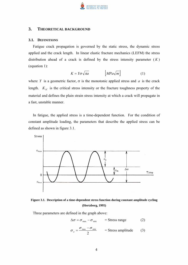
3. THEORETICAL BACKGROUND

3.1. DEFINITIONS

Fatigue crack propagation is governed by the static stress, the dynamic stress

applied and the crack length. In linear elastic fracture mechanics (LEFM) the stress

distribution ahead of a crack is defined by the stress intensity parameter ( K )

(equation 1):

aYK πσ= [ ]mMPa (1)

where Y is a geometric factor, σ is the monotonic applied stress and a is the crack

length. ICK is the critical stress intensity or the fracture toughness property of the

material and defines the plain strain stress intensity at which a crack will propagate in

a fast, unstable manner.

In fatigue, the applied stress is a time-dependent function. For the condition of

constant amplitude loading, the parameters that describe the applied stress can be

defined as shown in figure 3.1.

Figure 3.1. Description of a time-dependent stress function during constant amplitude cycling

(Hertzberg, 1995)

Three parameters are defined in the graph above:

minmax σσσ −=∆ = Stress range (2)

2minmax σσ

σ−

=a = Stress amplitude (3)

5

2minmax σσ

σ+

=m = Mean stress (4)

max

min

σσ

=R . = Stress ratio (5)

When the tensile and compressive components of the cyclic stress have the same

magnitude R is equal to -1. This is the case for rotating bending fatigue where every

portion of the surface of the shaft is subjected to the same stress cycle during one

revolution. Turbine rotors and other rotating shafts are subjected mainly to this type

of stress as a result of bending under the shaft’s own weight. The shaft will also be

subjected to a cyclic shear stress during every revolution. In addition, the turbine

shaft also transmits torque and is therefore also subjected to a torsional stress of

approximately constant value.

The cyclic stress intensity range )( K∆ for a constant cyclic stress amplitude can be

defined as the difference between the maximum and the minimum stress intensities

during fatigue when the crack length is a. Therefore:

aYKKK πσ∆=−=∆ minmax (6)

where maxK is the maximum stress intensity and minK the minimum stress intensity

during the loading cycle. The effective stress intensity range effK∆ can be defined as

the stress intensity range that is the driving force for crack propagation:

opeff KKK −=∆ max (7)

where opK represents the stress intensity at which the crack faces first separate as the

stress is increased during the load cycle.

In the calculation of K∆ it is customary and convenient to assume that only the

tension part of the cycle contributes to the crack propagation during the fatigue

process. If the loading cycle has a compressive component, the crack faces will be

pressed together; as far as crack propagation is concerned, this portion of the stress

cycle is frequently disregarded by assuming 0min =K and therefore maxKK =∆ .

However, the influence of the compressive portion of the load cycle cannot be

disregarded altogether as is seen from the literature survey.

6

The fatigue crack growth rate per cycle (dNda ), in mm/cycle, resulting from a cyclic

stress intensity range ( K∆ ) is determined by measuring the average crack growth for

a fixed number of stress cycles. Figure 3.2 is a representation of typical crack growth

data where the crack length is recorded as a function of the number of fatigue cycles.

Figure 3.2. Crack growth data at two different cyclically applied stresses (Hertzberg, 1995)

The fatigue crack growth rate (FCGR) is usually determined by using the tangent

to the crack growth curve or by an incremental polynomial method described in

ASTM 647-99. It is seen from the figure above that for the same crack length, the

FCGR is higher when the cyclic stress range is larger.

Crack growth rate data can then be graphically presented as a function of the cyclic

stress intensity range ( K∆ ) on a log-log scale plot. The general features of such a

curve are shown in figure 3.3. The curve has a sigmoidal shape with two asymptotes

terminating the curve at very high and at very low stress intensity ranges.

7

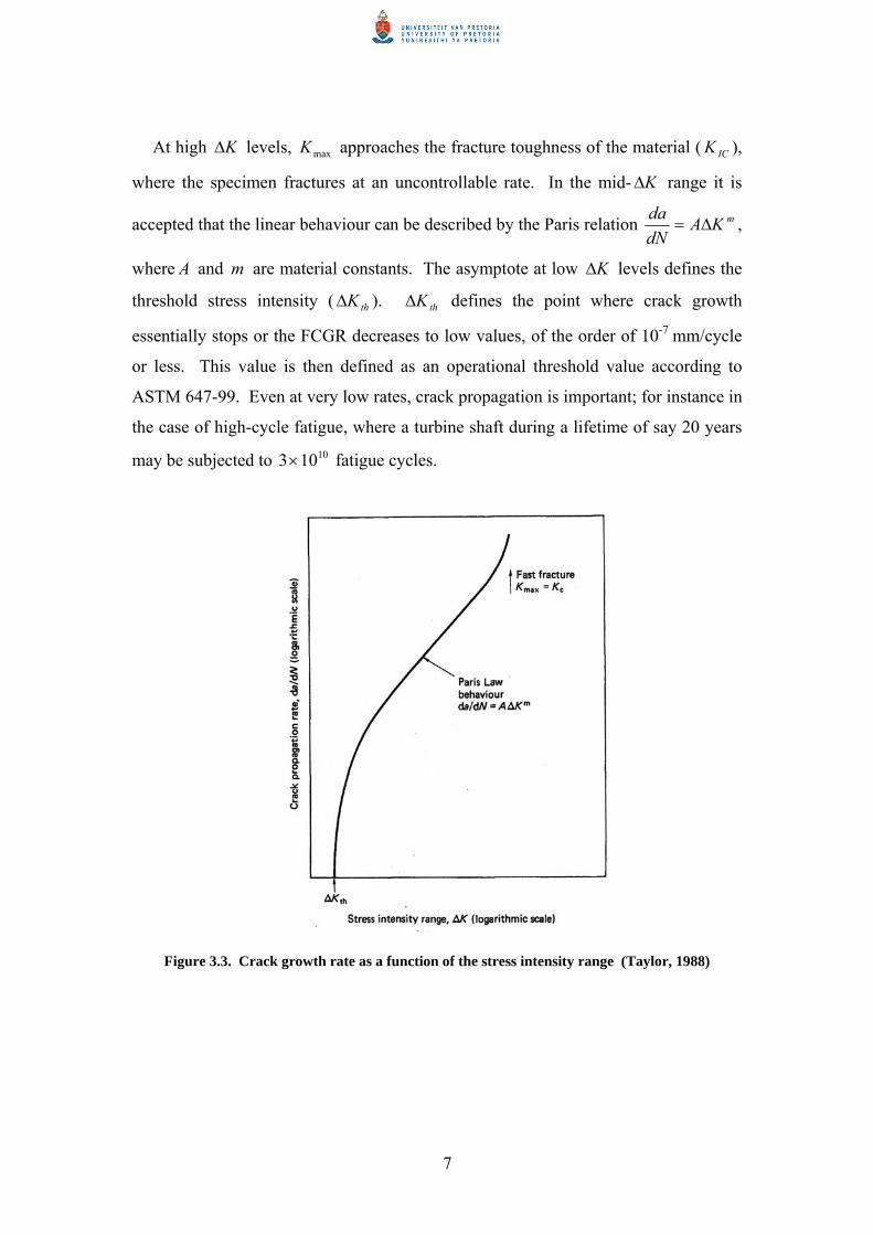
At high K∆ levels, maxK approaches the fracture toughness of the material ( ICK ),

where the specimen fractures at an uncontrollable rate. In the mid- K∆ range it is

accepted that the linear behaviour can be described by the Paris relation mKAdNda

∆= ,

where A and m are material constants. The asymptote at low K∆ levels defines the

threshold stress intensity ( thK∆ ). thK∆ defines the point where crack growth

essentially stops or the FCGR decreases to low values, of the order of 10-7 mm/cycle

or less. This value is then defined as an operational threshold value according to

ASTM 647-99. Even at very low rates, crack propagation is important; for instance in

the case of high-cycle fatigue, where a turbine shaft during a lifetime of say 20 years

may be subjected to 10103× fatigue cycles.

Figure 3.3. Crack growth rate as a function of the stress intensity range (Taylor, 1988)

8

3.2. RELEVANT TERMS

The loading mode describes the geometric orientation of the crack faces relative to

the orientation of the applied stress. Figure 3.4 shows the three basic modes of

loading.

Figure 3.4. Different loading modes (Hertzberg, 1995)

In the case of rotating bending where the cyclic shear stress is zero (pure bending

moment), crack propagation occurs in the crack opening mode (Mode I) and crack

propagation can be expected when the bending stress at a particular point reaches a

maximum tensile value. Crack propagation will always occur at right angles to the

direction of the principal tensile stress, and consequently the crack orientation at the

surface can be expected to be transverse to the longitudinal direction of the shaft when

the shear stress and torsional moment are zero. This will, however, be affected by the

presence of a torsional moment and the cyclic shear stress to which the shaft may be

subjected. At the maximum crack opening orientation, the stress condition the surface

can be illustrated with a Mohr circle (figure 3.5).

9

Figure 3.5. Mohr circle representing the stress in the maximum crack opening orientation

( bσ = bending stress and sτ = torsional shear stress)

In the presence of shear loading, crack propagation can then be expected along a

helical path oriented at an angle θ with respect to the transverse direction. As a

fatigue crack propagates when the cyclic shear stresses due to shear forces are no

longer negligible in comparison with the bending stress, the increasing magnitude of

the cyclic shear stress will also affect the orientation of the crack and cause the angle

θ to increase further. The situation is further complicated by possible crack

propagation in the crack tearing mode (Mode III) when the shaft with a crack has

turned through a further 90º from the fully crack opening position. This can in some

instances result in a crack surface with an increasingly ratcheted surface as the crack

progresses towards the centre of the shaft.

Crack closure is a term used to describe the condition when there is an obstruction

in the crack wake that prevents the crack faces from separating immediately when the

applied stress is increased. Crack closure therefore reduces the effective cyclic stress

intensity ( effK∆ ). Crack closure therefore reduces the portion of the cyclic stress

amplitude when the crack faces are apart and the crack is consequently able to

maxσ

10

propagate. There are three main crack closure mechanisms that influences fatigue

threshold behaviour:

Plasticity-induced crack closure occurs when the compressive residual stress of

the plastic zone that forms in front of the crack tip during unloading produces crack

closure, preventing the crack from extending. This is particularly the case when an

overload fatigue cycle is followed by regular fatigue crack testing at a lower cyclic

stress.

Roughness- or asperity-induced crack closure occurs when the fracture facets on

opposite crack faces do not fit well when the crack faces close as the applied stress is

decreased. Evidence of this is when rubbing of the crack faces result in a shiny

fracture surface. This type of behaviour can be expected when there are complex

movements of the crack faces such as may be expected during rotating bending where

there are also high cyclic shear stresses due to shear forces and torsional moments.

Oxide- or debris-induced crack closure is found when some extraneous material,

usually corrosion or oxidation products, is present in the crack wake preventing the

crack from fully closing again after incremental crack propagation.

11

4. LITERATURE SURVEY

The threshold cyclic stress intensity ( thK∆ ) at the operating temperature is of

critical importance in assessing the reliability with which a turbine shaft can be

operated. If the cyclic stress intensity range is less than the threshold value, further

crack propagation is not expected. To obtain reliable values, testing would have to be

done with a loading cycle that simulates the cycle to which the shaft is subjected in

practice. At the same time it would require the experiments to be done in a steam

environment at operating temperatures and pressures. Whereas it is feasible to do

experiments in a steam atmosphere at various temperatures at atmospheric pressure,

conducting experiments at the pressures encountered in a steam environment is much

more difficult. As a first approximation to simulate real operating conditions,

experiments can be conducted at the operating temperature but at atmospheric

pressure, provided the steam is superheated.

4.1. ENVIRONMENT

In a study by Tu & Seth (1978) on the effect of a steam environment at 260 °C, it

was found that thK∆ was higher than in air at the same temperature (figure 4.1). The

increase is attributed to an embrittlement process that causes crack branching, which

in turn reduces the crack tip driving force. This embrittlement process is mentioned

as opposed to blunting, which is a dissolution process at the crack tip. Branched

cracks were found in the fast crack growth region as well as in the threshold region,

although to a lesser extent in the latter region. In the case of testing in the steam

environment a black corrosion product formed on the crack faces. It was argued that

the dense corrosion product may reduce the diffusion of steam to the crack front,

thereby reducing crack branching in the near-threshold region. The influence of the

steam environment can be due to both the nature of the oxide that forms at the crack

tip as well as modification of the mechanism of crack propagation when crack

branching occurs. The view was expressed that crack branching probably has a much

larger effect than the crack closure effects due to the presence of oxides.

12

Figure 4.1. The influence of steam and air at 260 °C on thK∆ (Tu and Seth, 1978)

In another study (Smith, 1987) on a 2NiCrMoV rotor steel in moist air and in dry

air environments respectively at room temperature with 14.0=R , it was found that

thK∆ was higher for the moist air environment than for the dry air environment. This

in turn was attributed to the formation of oxide debris near the threshold region

causing oxide-induced crack closure (figure 4.2). In the same study the fatigue

thresholds were first determined separately for both dry and moist air environments.

In a subsequent test the effect of a change from dry to moist to dry air was studied

using a constant K∆ value, with thK∆ dry air < K∆ < thK∆ moist air. It was found that the

crack growth rate in dry air first followed the dry air curve, but when the moist air

was admitted crack growth was arrested, even after dry air was subsequently

readmitted. From this it appears that once a fatigue threshold has been established in

13

a specific environment, further crack propagation will not take place when the

environment is subsequently changed to an environment with a lower fatigue

threshold. This is probably due to the fact that the crack closure effect due to the

moist environment is maintained even after the environment is changed to dry air.

Figure 4.2. The influence of moist air and dry air for 2NiCrMoV steel on thK∆ (Smith, 1987)

The environmental effects in different dry and moist environments were also

evaluated for bainitic 2.25Cr-1Mo pressure vessel steel with 05.0=R at room

temperature (Suresh and Ritchie, 1983). Air was used as a reference for subsequent

experiments in distilled water, wet hydrogen and dry hydrogen. It was found that for

all the wet environments, including hydrogen, thK∆ was higher than in a dry

(hydrogen) environment (figure 4.3). The corrosion products on the fracture surface

were identified as Fe2O3. This is another example of oxide debris wedging the crack

open and thus contributing to oxide-induced crack closure. Hydrogen-assisted

cracking can be ruled out, since even in wet hydrogen the threshold was higher than

that in dry hydrogen.

14

Figure 4.3. The influence of wet and dry environments on thK∆ (Suresh and Ritchie, 1983)

4.2. TEMPERATURE

Experiments in air at different temperatures have shown that thK∆ is dependent on

temperature. At elevated temperatures there is a temperature range where the

threshold stress intensity reaches a minimum value. This behaviour has been found in

both A508-3 steel (Kobayashi) and in a CrMoV steel (Liaw, 1985). Figures 4.4 and

4.5 show the results of Liaw and Kobayashi respectively. These experiments were

conducted over the temperature range of 24˚C to 427˚C. Liaw used a frequency of 60

Hz with 1.0=R and Kobayashi used 25 Hz with 05.0=R . Figure 4.6 summarises

Liaw's findings and explains the mechanisms underlying the temperature effect.

15

Figure 4.4. The effect of temperature on thK∆ (Liaw, 1985)

Figure 4.5. The effect of temperature on thK∆ (Kobayashi et al, 1991)

The following reason was advanced for this behaviour. At room temperature thK∆

is high due to a rougher fracture surface which interferes during the closing part of the

cycle to cause roughness-induced crack closure. At intermediate temperatures, i.e.

~150˚C, thK∆ reaches a minimum value due to the formation of a stable thin oxide

layer on the crack faces and a reduction in surface roughness. In the high-temperature

region the oxide layer thickness increases again due to thermal oxidation that

produces crack closure and then results in higher thK∆ values. This is schematically

illustrated in figure 4.7.

16

Figure 4.6. Summary of the effect of temperature on thK∆ (Liaw, 1985)

Figure 4.7. Diagrammatical illustration of the temperature effect on thK∆ (Kobayashi, 1991)

17

4.3. STRESS RATIO ( R )

The general trend observed in stress ratio studies is that as R is increased, thK∆

decreases. As stated earlier, R is a measure of the mean applied stress. The

influence of R can also be explained by the concepts of crack closure. At the low

end of R oxide- and roughness-induced crack closure dominate, since the crack faces

come into close contact. However, at the high end of R the effect of crack closure is

reduced due to the high mean loads causing the crack faces to stay apart and therefore

reducing the crack closure effect.

An example of the influence of R on thK∆ is seen in a study (Suresh and Ritchie,

1983) where 75.005.0 ≤≤ R was used in an air environment at room temperature for

an SA542-3 steel (figure 4.8). The same trend can be seen in figures 4.4 and 4.5.

Figure 4.8. The influence of R on thK∆ ( Suresh and Ritchie, 1983)

Usually crack propagation tests are conducted with 0≥R . In the case of rotating

bending 1−=R , and it is important also to know what happens at negative values of

R . The influence of negative R values is shown in figure 4.9 (Lindley, 1981). The

solid lines for 0<R represent the possible condition where minK is taken as negative

for the compressive part of the cycle. This will cause K∆ to become larger and

consequently result in an increase of thK∆ as R becomes more negative. On the

18

other hand, the dashed lines represent the usual dependence of thK∆ on R as

maxKK =∆ with 0min =K for the compressive part of the cycle.

Figure 4.9. The effect of stress ratio on thK∆ , with negative values of R (Lindley, 1981)

4.4. COMPRESSIVE LOADS

During rotating bending fatigue, one half of the stress cycle is compressive and the

other half tensile. According to ASTM 647-99, it is recommended that only the

tensile part of the load cycle be taken into consideration in the calculation of K∆

neglecting the compressive half of the cycle. A number of studies investigating the

influence of the compressive portion of the loading cycle suggest that this assumption

could lead to non-conservative predictions of thK∆ obtained from testing where

0min =K . In these studies, it was found that the magnitude of the compressive stress

cycle as well as the number of cycles between compressive stress cycles has an

influence on thK∆ .

In a study by Zaiken et al (1985) using I/M 7150 aluminium alloy in the

underaged-, peak and overaged condition thresholds were first determined with

19

1.0=R . Thereafter a single compressive load was applied and the test was resumed

at thKK ∆=∆ with 1.0=R . It was observed that further crack growth occurred

subsequent to the single compressive load cycle (figure 4.10). Further crack growth

stopped after the crack had progressed by 60 to 170 µm, depending on the ageing

condition. It was found that compressive loads down to max3 K× did not result in

further crack growth. Only when the compressive cycle was equal to max5 K× was

there an effect. The same observations were also made for SAE1010 steel. One

sample was used to determine a reference crack growth rate curve with 0=R . The

second sample was then cycled at a low K∆ value, also with 0=R , and gave an

FCGR similar to the reference curve. Three compressive load cycles were then

applied with a magnitude equal to max3 K× , after which the test was resumed. The

FCGR increased relative to that of the reference curve, and only after 51067.6 ×

further cycles did the FCGR decrease to the original value of the reference curve.

A saturation compressive cycling effect was reported for Cu and two Al alloys in a

study (Kemper et al, 1989) where thK∆ was determined with R ranging from 10− to

8.0+ defining maxKK =∆ for 0<R and minmax KKK −=∆ for 0>R . Decreasing

the value of R towards more compressive loading did not decrease thK∆ beyond a

certain limit, as shown for Cu in figure 4.11. In all the samples, this saturation limit

was found to occur at 2−≈R . The reduction in the threshold stress intensity values

as R becomes more negative was attributed to the reduction of roughness-induced

crack closure due to the plastic flattening of asperities during the compression portion

of the cycle.

20

Figure 4.10. Increase in the crack growth rate (closed symbols) when cycled at thKK ∆=∆

with 1.0=R after a single max5 K× compressive load for underaged (UA), peak aged (PA) and

overaged (OA) 7150 Al alloy samples (Zaiken et al, 1985)

Figure 4.11. Influence of stress ratio on the fatigue threshold of recrystallised Cu (Kemper et al,

1989)

21

For Waspaloy, an aluminium powder metallurgy alloy IN-9052 and bearing steel

M50NiL (Carlson et al, 1994) it was found that the crack growth rate increased

sharply when the stress ratio was changed to 2−=R after cycling at 1.0=R . The

above study did not consider compressive stress cycle effects on the threshold stress

intensity value, but focused on the influence of compressive stress cycle effects on

FCGR (loading sequence shown in figure 4.12). There is a clear indication that

compressive cycling increases the crack growth rate for a given K∆ when minK∆ is

defined as 0min ≥∆K . This behaviour was attributed to the inelastic crushing of

asperities, resulting in a decrease of roughness-induced crack closure.

Figure 4.12. Loading sequence to assess crack growth behaviour of alternate compressive load

cycling (Carlson et al, 1994)

Topper et al (1985) investigated the effect of intermittent compressive stress cycles

on aluminium and steel. It was found that as the number of cycles between successive

compressive stress cycles during a test with 0=R increased, the threshold value

increased (see Figure 4.13). When the number of compressive stress cycles during the

test was zero, the threshold thK∆ was at a maximum value, but when compressive

stress cycles were applied during each cycle the threshold decreased to a minimum

value. In CSA G40.21 steel, thK∆ decreased from mMPa2.7 for no compressive

22

stress cycles to mMPa5.3 when each cycle contained a compressive stress cycle

component as shown in figure 4.13.

Figure 4.13. Decreasing the interval between compressive stress cycles decreases thK∆ in CSA

G40.21 steel (Topper et al, 1985)

From this it is concluded that compressive stress cycles also influence thK∆ ,

especially if crack closure is a dominant feature. If a material does not exhibit a large

crack closure effect (for instance when it has a very small grain size), the ASTM

recommendation would apply, since the compressive stress cycle – within limits –

then does not influence the effective stress intensity to any large extent.

23

4.5. RESIDUAL STRESS

Because of the difficulties encountered in measuring residual stress fields (Lawson

et al, 1999), the literature on the influence of residual stresses on thK∆ is not very

extensive. However, residual stress fields can be expected to influence the FCGR.

The threshold value in particular is very sensitive to any change in effK∆ . The nature

of the plastic zone formed during the fatigue loading sequence of a crack also results

in a local residual stress system that would be modified by the longer-ranging original

residual stresses. Upon unloading after a tensile overload, for example during fatigue,

the stress state around the crack tip results in a larger zone with a very high

compressive stress. When cycling is resumed at the previously lower stress intensity

range, the crack growth is retarded, and the original crack growth per cycle is only

reached after the crack has proceeded beyond the compressive stress field set up by

the overloading. If the applied stress intensity is not large enough to cancel the

compressive stress field, the crack could arrest completely. This effect is also

observed when threshold values are artificially high because the load-shedding rate

which causes plasticity-induced crack closure is high.

Residual stress fields have a marked influence on the profile (shape) of the fatigue

crack front, illustrating the influence they can have on thK∆ and to a lesser extent on

K∆ . This behaviour was observed in a study by Geary et al (1987) investigating the

influence of tempering temperature on a quenched and tempered low alloy boron

steel. Figure 4.14 shows the measured residual stress distribution across the

specimen, while figure 4.15 shows the actual crack front profile at the threshold. As

an approximation, the residual stress field can be considered to be superimposed onto

the applied stress field, changing the local value of R .

24

Figure 4.14. Measured residual stress distribution across a quenched and tempered specimen

(Geary et al, 1987)

Figure 4.15. Actual crack front profile of a specimen austenitised at 900 °C, quenched in water

and tempered at 20 °C (Geary et al, 1987)

4.6. TEST CYCLE FREQUENCY

It has been shown (Bignonnet et al, 1982) that there is a decrease in the threshold

stress intensity with decreasing test frequency. In tests conducted in air at room

25

temperature, fretting oxidation was advanced as the mechanism to explain the

increase of the FCGR at higher test frequencies. Although the near-threshold

condition was not considered, an extrapolation of their results for testing at 65Hz and

7Hz would probably result in a higher threshold value for 65Hz compared with a

threshold value for 7Hz (figure 4.16).

Figure 4.16. Effect of test frequency on the fatigue crack growth rate (Bignonnet et al, 1982)

4.7. GRAIN SIZE

Grain refinement has been used to increase the strength as well as the fatigue limit

of materials. This effect is thought to be due to an increase in the number of obstacles

that will retard crack initiation. However, this is not the case during near-threshold

crack propagation, where thK∆ increases with the grain size (Lawson et al, 1999).

Data in the literature (Lindley, 1981) indicates that lower-strength steels in general

have a higher threshold value than high-strength steels (figure 4.17). The influence of

grain size on thK∆ can be explained partially by the fact that the strength of the steel

increases as the grain size decreases. A decreased grain size can also produce a

smoother fracture surface and therefore have less of a crack closure effect.

26

Figure 4.17. Collective threshold data for high- and low strength steels as a function of R

(Lindley, 1981)

In a study by Masounave et al (1976) on a ferritic steel it was shown that the effect

on thK∆ is directly proportional to the square root of the grain size, as shown in figure

4.18.

Figure 4.18. Effect of grain size on the threshold stress intensity (Masounave et al, 1976)

27

4.8. CONCLUSION

From the literature search it can be concluded that most of the thK∆ effects can be

related to crack closure mechanisms. If the environment is high-temperature steam,

the mechanism seems to be branching of the crack front (Tu & Seth, 1978) as well as

a buildup of corrosion products, both of which decrease the effective stress intensity.

In steam a higher resistance to crack propagation is expected and consequently also a

higher fatigue threshold value.

28

5. MACHINE DESIGN

5.1. ROTATING BENDING

Rotating bending is normally carried out with RR Moore-type rotating bending

machines (Czyryca, 1985), in which the gauge length of the specimen is subjected to a

pure bending moment. The cyclic stress in a rotating shaft can, for example, also be

simulated by suspending a dead load from the free end of the rotating shaft. At the

position where the specimen fails the material will – apart from a cyclic bending

stress – also be subjected to a smaller cyclic shear stress. To establish the fatigue

threshold stress intensity, the bending moment on pre-cracked specimens is reduced

until a point is reached where the specimen never breaks. Although the setup is

simple, it is expensive and time consuming due to the large number of samples

required.

Uniaxial servo-hydraulic machines, in a way, simulate rotating bending when the

stress ratio (R) is equal to -1. These types of tests do not fully mimic the shear

interaction of the crack faces during rotating bending, where large cyclic shear

stresses may also be present. One of the disadvantages of the above method is the

presence of mechanical backlash in the setup as the load passes the zero load line

from tension to compression. Another disadvantage is that misalignment can easily

result from buckling of the sample during the compressive part of the cycle.

Consequently, a need exists for a machine that can simulate the complex crack face

movement encountered during rotating bending of an actual shaft and also allows

continuous crack measurement.

For this purpose it was necessary to design and build a customised fatigue-testing

machine. The design provides for a round specimen that is rigidly clamped at the one

end whilst the other end is subjected to a circular motion by means of an eccentric

drive. The aim of this design is to produce a loading sequence of tension and

compression, at the tip of the crack, of equal magnitude; this means that 1−=R . The

fact that the specimen itself does not rotate enables the continuous monitoring of

crack propagation during testing.

29

5.2. DESIGN OF FATIGUE TESTING MACHINE SIMULATING ROTATING BENDING

Figure 5.1 shows the custom-built fatigue-testing machine on the left with its steam

generating system at top right.

Figure 5.1. Setup of the fatigue-testing machine

Figure 5.2 is an isometric drawing of the machine setup.

Electric motor

Frame

Eccentric drive

Specimen shaft

Cover plate

Steam generation

30

Figure 5.2. Isometric drawing of the machine setup

Legend (Figure 5.2):

A = 3 kW 1450 rpm electric motor

B = Rectangular tubular frame

C = Eccentric drive

D = Self-aligning bearing (SKF No: 2209E-2RS1K TN9/C3)

E = Test shaft

F = Environmental chamber

G = Specimen fixture with side plates

H = Cover plates

I = Fixing bolt with washer

5.2.1. Frame

Figure 5.3 shows the frame consisting of a back plate with the electric motor bolted

to one side and rectangular tube legs welded to the opposite side. The whole

arrangement is supported by three double U-shear rubber mountings fixed to the floor.

A B

CD

E

F

G

H

I

31

Figure 5.3. Frame and electric motor

Figure 5.4 is the drawing of the frame.

Rectangular tubular legs

Eccentric drive

32

Figure 5.4. Drawing of the frame

5.2.2. Cantilever beam

Figure 5.5. Geometry of the cantilever specimen

Figure 5.6 is a drawing of the cantilever beam.

Figure 5.6. Drawing of the cantilever specimen with wire cut slit

10 mm wire cut slit

Double U-shear vibration damping mountings

Rectangular tube Cover plates Side elevation

Plan

33

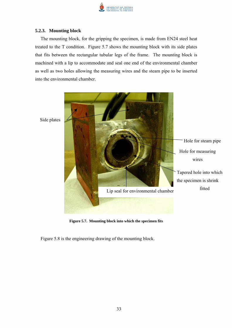
5.2.3. Mounting block

The mounting block, for the gripping the specimen, is made from EN24 steel heat

treated to the T condition. Figure 5.7 shows the mounting block with its side plates

that fits between the rectangular tubular legs of the frame. The mounting block is

machined with a lip to accommodate and seal one end of the environmental chamber

as well as two holes allowing the measuring wires and the steam pipe to be inserted

into the environmental chamber.

Figure 5.7. Mounting block into which the specimen fits

Figure 5.8 is the engineering drawing of the mounting block.

Side plates

Lip seal for environmental chamber

Hole for measuring

wires

Hole for steam pipe

Tapered hole into which

the specimen is shrink

fitted

34

Figure 5.8. Drawing of the mounting block

5.2.4. Eccentric drive

Figure 5.9 shows the eccentric drive made from EN24 steel heat-treated to the T

condition. The figure also shows the machined grooves for adjusting the eccentricity

as well as the three grub screws to keep the bearing sleeve in place. The measurement

tape in the figure indicates the eccentricity to which the eccentric drive is set.

Reference points, of zero eccentricity, are marked on the outer surface of the eccentric

drive. The deflection of the specimen is related to the relative setting of the

references points on the outer surface which is indicated by the measurement tape.

The specimen with the fitted self-aligning bearing fits into the sleeve as shown at the

bottom of the figure while the side of the eccentric drive with the grooves (top of

figure) is fixed to the shaft of the electric motor.

35

Figure 5.9. Eccentric drive to apply the load. The eccentricity is indicated by the arc length

setting using the tape measure

Figure 5.10 shows details of the eccentric drive.

Bearing sleeve

Grooves for adjusting the eccentricity

Eccentricity indicationGrub screws

Self-aligning ball bearing

(fits into the bearing sleeve)

Bearing sleeve

36

Figure 5.10. Drawing of the eccentric drive

5.2.5. Accessories

Figure 5.11 shows the accessories to adjust the eccentric drive. The 8 mm Allen

key is used to undo the three grub screws, then the M8 bolt is inserted into one of the

grub screw holes and is pushed against the inside of the rectangular tube leg of the

frame while the C-key is used to adjust the eccentricity to the desired arc length

according to eccentric indicator, at which position it is then fixed by tightening the

grub screws.

Figure 5.11. Accessories to set the eccentric

C-key

Alan-key

M8 bolt

37

5.3. ENVIRONMENTAL CHAMBER

A 1000 Watt electrically heated environmental chamber was built (shown in figure

5.12) for the high-temperature air and high-temperature steam tests.

Figure 5.12. The environmental chamber to heat the cantilever beam

Figure 5.13 shows the details of the environmental chamber.

38

Figure 5.13. Drawing of the environmental chamber

The main chamber is manufactured from a mild steel pipe. Mica sheet is wrapped

around the outer surface of the pipe to electrically insulate the Nichrome ribbon

heating element wire. The element windings are kept in place by alumina cement.

The space between the chamber and the stainless steel case is thermally insulated with

silica wool. The environmental chamber successfully controlled the specimen

temperature to within 1 ºC of the set temperature. The steam that was admitted to the

environmental chamber was sealed with a specially moulded high-temperature silicon

rubber cup that was clamped to the specimen and chamber by circular clamps.

Sufficient positive steam pressure was maintained inside the environmental chamber

to maintain an outward steam flow and to prevent atmospheric air leaking into the

chamber.

5.4. STEAM GENERATION SYSTEM

Steam was generated using a hotplate and a boiler that is open to the atmosphere.

Distilled water is fed into the boiler via a 20 m head pressure pipe as shown in figure

39

5.14. The control system for the water feed is simple and works on a mass balancing

principle. The control valve is a metal plate that pushes down onto a flexible silicone

tube. As water fills the boiler, the controller valve closes. As steam escapes the valve

opens to let in small amounts of water to restore the balance. The energy input to the

hotplate controls the amount of steam that is evaporated into the environmental

chamber. The steam that is created in the boiler is above 100 °C due to the

constricted outlet from the boiler. This increases the pressure above atmospheric,

causing the water to boil at 117 °C. Should the system generates steam too fast, due

to an excessive hotplate energy input, the pressure would increase and the inlet water

be pushed back into the distilled water reservoir, causing the system to run dry. In

order to maintain a positive pressure in the environmental chamber and eliminate the

possibility of air entrainment, an evaporation rate of 0.3 ml water/s was found to be

adequate.

Figure 5.14. The steam generation system

Silicone tube

40

6. EXPERIMENTAL WORK

6.1. MATERIAL

Low carbon steel was used during testing. The composition is shown in Table 6.1

and the microstructure in figure 6.1. A stress-relieving heat treatment at 650 °C for 5

hours was performed to relieve any residual stress in the specimen that could

influence crack propagation. The average measured grain size was 30µm.

Table 6.1. Chemical composition of the steel used

Al As B C Ca Cr Cu Fe Mn

0% 0.00% 0.00% 0.12% 0.00% 0.03% 0.11% Bal 0.57%

Mo Nb Ni P S Si Sn Ti V

0.01% 0.00% 0.09% 0.01% 0.03% 0.16% 0.01% 0.00% 0.00%

Figure 6.1. Microstructure of the low carbon steel that was used in experiments

41

6.2. ASSEMBLY OF THE MACHINE

The assembly sequence required for testing was as follows: first the specimen has

to be fitted into the mounting block by cooling the tapered end of the cantilever beam

in a mixture of ethanol and dry ice while heating the mounting block in a convection

oven, thus obtaining a very tight shrink fit when they are bolted together. The crack

measurement and the thermocouple wires were then spot welded into place after

which the environmental chamber was positioned over the specimen, fitting into the

groove on the mounting block. An airtight joint was achieved by means of a silicone

sealant. The other side of the environmental chamber was sealed onto the specimen

by a specially moulded silicone cup and circular metal clamps. The self-aligning

bearing was then fitted to the free end of the cantilever beam. This subassembly was

positioned between the legs of the frame with the bearing fitting into the eccentric

drive set at zero eccentricity. The assembly was completed by securing the mounting

block with side bolts and the cover plate. The holes of the measuring wires as well as

the steam pipe were fully sealed with silicone rubber at the point of exit on the

mounting block.

6.3. CRACK MEASUREMENT

6.3.1. Crack measurement calibration

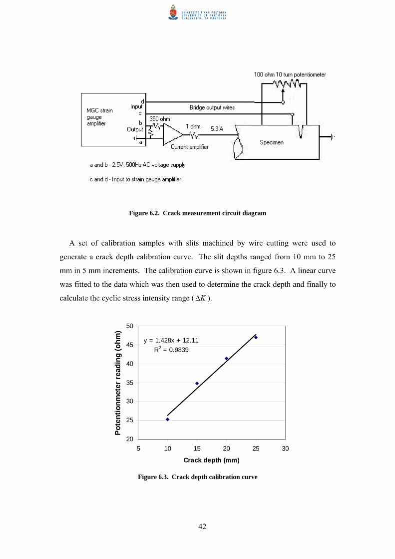
Crack measurement was done by means of a modified Wheatstone bridge and

measurements were logged on a computer using Catman software for the MGC strain

gauge amplifier. Figure 6.2 shows the crack measurement setup. The AC voltage

output from the strain gauge amplifier was amplified by a current amplifier to pass an

AC current of 5.3 amps through the specimen. Initially the bridge was balanced by

adjusting the 10-turn potentiometer. The electrical resistance of one leg of the bridge

increased as the crack length increases. This caused the bridge to become

unbalanced; it was rebalanced by adjusting the potentiometer. For each crack length

there was a corresponding precision 10-turn potentiometer reading on the 10-turn dial

indicator. The advantage of this circuit was that it compensated for resistance

changes due to any variation in temperature as well as any change in the current from

the current amplifier.

42

Figure 6.2. Crack measurement circuit diagram

A set of calibration samples with slits machined by wire cutting were used to

generate a crack depth calibration curve. The slit depths ranged from 10 mm to 25

mm in 5 mm increments. The calibration curve is shown in figure 6.3. A linear curve

was fitted to the data which was then used to determine the crack depth and finally to

calculate the cyclic stress intensity range ( K∆ ).

y = 1.428x + 12.11R2 = 0.9839

20

25

30

35

40

45

50

5 10 15 20 25 30

Crack depth (mm)

Pote

ntio

nmet

er re

adin

g (o

hm)

Figure 6.3. Crack depth calibration curve

43

Spot welding was used to secure all the wires on the specimen as well as on the

crack depth calibration samples. Constantan wires 0.1 mm and 0.3 mm in diameter

were used for potential and current conductors respectively to produce strong spot

welds. The separate current conductors were spot welded as shown in the figure 6.4;

one at 15 mm from the slit and the other at 65 mm on the opposite side of the slit.

Potential conductors were spot welded as near as possible on opposite sides of the slit

whilst the other bridge wire was spot welded 45 mm from the slit.

Figure 6.4. Depiction of the spot weld points

6.3.2. Crack measurement during testing

The accuracy of crack measurements was also checked by comparing the electrical

measurements to optical measurements of the crack depth when the fatigue-cracked

faces of the specimen were finally opened up after termination of the experiment. It

was found that the difference was less then 6.2 % as long as the crack geometry

stayed fairly flat without excessive curvature (see Table 6.2).

Table 6.2. Accuracy of the electrical measurement system

Sample Optical Electrical % AccurateAir 24 ºC 15.88 15.85 99.81

Air 160 ºC 18.54 18.3 98.71Steam 160 ºC 17.45 16.37 93.81

Measured crack length (mm)

44

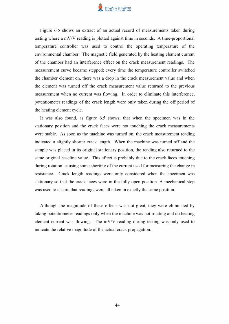
Figure 6.5 shows an extract of an actual record of measurements taken during

testing where a mV/V reading is plotted against time in seconds. A time-proportional

temperature controller was used to control the operating temperature of the

environmental chamber. The magnetic field generated by the heating element current

of the chamber had an interference effect on the crack measurement readings. The

measurement curve became stepped; every time the temperature controller switched

the chamber element on, there was a drop in the crack measurement value and when

the element was turned off the crack measurement value returned to the previous

measurement when no current was flowing. In order to eliminate this interference,

potentiometer readings of the crack length were only taken during the off period of

the heating element cycle.

It was also found, as figure 6.5 shows, that when the specimen was in the

stationary position and the crack faces were not touching the crack measurements

were stable. As soon as the machine was turned on, the crack measurement reading

indicated a slightly shorter crack length. When the machine was turned off and the

sample was placed in its original stationary position, the reading also returned to the

same original baseline value. This effect is probably due to the crack faces touching

during rotation, causing some shorting of the current used for measuring the change in

resistance. Crack length readings were only considered when the specimen was

stationary so that the crack faces were in the fully open position. A mechanical stop

was used to ensure that readings were all taken in exactly the same position.

Although the magnitude of these effects was not great, they were eliminated by

taking potentiometer readings only when the machine was not rotating and no heating

element current was flowing. The mV/V reading during testing was only used to

indicate the relative magnitude of the actual crack propagation.

45

Figure 6.5. Extract of an actual record of measurements taken during testing

6.4. LOADING

The amplitude of the cyclic applied stress can be changed by adjusting the degree

of eccentricity. For this purpose, part of a measuring tape was glued to the eccentric

drive to indicate the arc length, as shown in figure 5.10. The actual strain at the

location of the fatigue crack at any particular arc length setting was established by

glueing a strain gauge to a test shaft without a slit at the position where the actual slit

would be. From the amplitude of the strain value, the applied stress was calculated

using a value of E = 205 GPa. This was then used as a calibration to calculate the

cyclic stress intensity range during the remainder of the testing, as shown in figure

6.6. The loading cycle frequency was 24 Hz.

Machine running

Machine running Machine stationary

Potentiometer zero balancing

Stepped curve dueto on/off heating cycle

Dynamic shift due tocrack faces makingcontact during thecompressive cycleduring testing

46

y = 0.0096xR2 = 0.9979

0.25

0.3

0.35

0.4

0.45

0.5

30 35 40 45 50

Arc length (mm)

Stra

in r

ange

(mm

/m)

Figure 6.6. Strain calibration curve indicating the strain range in relation to the eccentric arc

length

6.5. EXPERIMENTAL

In the initial tests it was found that it was not possible to fix the specimen rigidly

by tightening the end bolt alone; the specimen rocked and also slowly rotated in the

fixture. To stop this, the tapered end was then pressed into the tapered hole with a

press. This apparently resulted in some plastic yielding at the tip of the slit and non-

uniform residual stress distribution that affected the crack propagation per cycle and

also the shape of the crack front. These subsequent experiments were also not

satisfactory and resulted in fatigue crack fronts that were highly asymmetrical relative

to the orientation of the slit (see figure 7.11 in Section 7.6). Finally, the shrink fitting

procedure described previously solved the problem, thereafter the fatigue crack front

propagated reasonably symmetrically relative to the position of the starter notch.

After all the experimental problems had been solved, samples were first tested in

an air atmosphere at room temperature and at 160 °C, after which the threshold and

the crack propagation per cycle were evaluated in a superheated steam environment at

160 °C and atmospheric pressure.

47

6.6. DETERMINATION OF dNda / AND K∆

Experiments were started with a cyclic stress intensity at K∆ =10 mMPa , which

was then reduced in steps of 0.5 mMPa to avoid premature crack closure. A crack

extension of ± 0.5 mm was allowed before the next step to reduce K∆ was taken. At

near-threshold values ± 106 fatigue cycles were accumulated in order to accurately

determine the crack growth per cycle. At the threshold value 106 cycles were again

applied to ensure that no further crack propagation occurred. If no crack extension

occurred during the test period of 106 cycles, it was considered to be the valid

measured value of the threshold cyclic stress intensity ( thK∆ ).

The stress intensity range was calculated as follows:

aYEKKK πε2minmax

∆=−=∆

where 0min =K for rotating bending

E = Young’s modulus in GPa

ε∆ = Strain range as measured in the strain range calibration in mm/mm

a = Crack length in m

Y = Geometric factor

= 1 (for 45.02.0 ≤≤Da ; see figure 6.7)

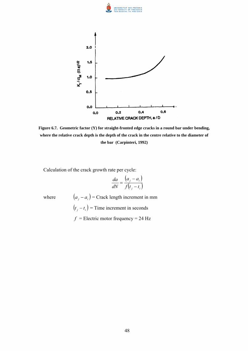
48

Figure 6.7. Geometric factor (Y) for straight-fronted edge cracks in a round bar under bending,

where the relative crack depth is the depth of the crack in the centre relative to the diameter of

the bar (Carpinteri, 1992)

Calculation of the crack growth rate per cycle:

( )( )ij

ij

ttfaa

dNda

−

−=

where ( )ij aa − = Crack length increment in mm

( )ij tt − = Time increment in seconds

f = Electric motor frequency = 24 Hz

49

7. RESULTS

7.1. CRACK GROWTH RATE VS. STRESS INTENSITY PLOTS

Using the data from tables 10.1 – 10.3 in appendix 10.1, the influences of

temperature and environment on crack propagation are shown in figure 7.1. The

results in figure 7.1 indicate that thK∆ in air at 24 °C was mMPa5.7 compared with

a value of only mMPa8.4 also in air but at 160 °C. In a superheated steam

environment at 160 °C the threshold value was again mMPa5.7 . However, at

higher cyclic stress intensities, the crack propagation per cycle was about one order of

magnitude lower than that in air at the same temperature. Experiments were only

performed once while all the data points for the respective curves were produced from

individual samples.

Figure 7.1. The influence of environment and temperature on thK∆ in mild steel

50

7.2. MACROSCOPIC FRACTURE SURFACES

In figures 7.2 – 7.4 the appearance of the fracture surfaces at the location of the

threshold can be seen. After the termination of an experiment the crack was opened

up by way of sawing into the back ligament and forcing the crack to open with a

hammer. In all these figures the starter notch can be seen starting at the top edge of

the round bar, extending 10 mm into the bar and ending in a straight line. The

reddish-brown colour, on the wire cut notch surface, is due to water that condensed

during the shrink fitting process described in Section 2.2.

Figure 7.2 shows that in the specimen tested in air at 24 °C a distinct dark grey

band of oxide formed in the vicinity of the threshold. The fracture surface was

relatively clean, with at best only a thin transparent oxide layer in the region where

the fatigue crack started and the crack propagation rate was high.

Figure 7.2. Fracture surface of the crack grown in air at 24 °C

In figure 7.3 similar features are visible for the fatigue crack propagating in air at

160 °C. In this instance the oxide that formed is scattered in patches over the fracture

surface. The oxide layer appears to become thicker as the threshold front is

Threshold

End of wire cut notch

Termination of experiment

51

approached. This is indicated by the darker blue appearance of the oxide in the

vicinity of the threshold.

Figure 7.3. Fracture surface of the crack grown in air at 160 °C

On the other hand, figure 7.4 shows that a dark black oxide layer formed uniformly

over the entire surface of the fatigue crack surface grown in steam at 160 °C.

Figure 7.4. Fracture surface of the crack grown in steam at 160 °C

Threshold

Threshold

52

7.3. TRANSVERSE SECTIONS OF CRACKS

Figures 7.5 – 7.7 show transverse sections of the fracture surface in the vicinity of

the threshold. The fracture surface for the specimen tested in steam at 160 °C appears

less rough than that of both the fracture surfaces of the specimens tested in air at

24 °C and 160 °C. The fracture surface of the specimen tested in air at 24 °C appears

to be the roughest. Yellow lines at the right hand side of these figures indicate the

vicinity of the threshold.

Figure 7.5. Transverse section perpendicular to growth direction in the vicinity of the threshold

in air at 24 °C. Arrow indicates the direction of crack propagation

Figure 7.6. Transverse section perpendicular to growth direction in the vicinity of the threshold

in air at 160 °C. Arrow indicates the direction of crack propagation

Figure 7.7. Transverse section perpendicular to growth direction in the vicinity of the threshold

in steam at 160 °C. Arrow indicates the direction of crack propagation

53

7.4. SCANNING ELECTRON MICROSCOPE IMAGES OF FRACTURE SURFACES

Figure 7.8 shows a scanning electron microscope (SEM) image of the fracture

surface tested in air at 24 °C. In the left-hand bottom corner of the image an oxide

layer with a dense appearance can be seen. At the top right-hand corner of the image

the exposed metal surface is visible. The fracture appearance of the metal surface

appears to be mixed, with both intergranular and transgranular features. It is

important to note that most of the metal surface is covered with oxide and that an

exposed metal surface is the exception, with only a few spots like those shown in

figure 7.8 in the vicinity of the threshold. It is probable that these patches may have

originated when the oxide layer was disturbed when the crack fracture surfaces were

opened up.

Figure 7.9 shows a SEM image of the fracture surface in the vicinity of the

threshold of the specimen tested in air at 160 °C. Unlike the fracture surface of the

test in air at 24 °C, the oxide in the top half of this image appears less dense and even

flaky. In the bottom half of the image the exposed metal surface is visible. In this

instance only transgranular features are visible.

Figure 7.8. SEM image of the oxide formed (bottom left) in the vicinity of the threshold in air at

24 °C. Arrow indicates the direction of crack propagation

54

Figure 7.9. SEM image of the oxide formed in the vicinity of the threshold in air at 160 °C.

Arrow indicates the direction of crack propagation

Figure 7.10 shows an image of the fracture surface near the threshold for the

specimen tested in steam at 160 °C. The whole surface was covered with a dense

hard magnetite (see Section 7.5.1) layer with a crystalline morphology, with no

exposed metal surfaces.

Figure 7.10. SEM image of magnetite formed in the vicinity of the threshold in steam at

160 °C. Arrow indicates the direction of crack propagation

55

7.5. CHARACTERISATION OF OXIDES

7.5.1. Oxide identification

Using the X-ray diffraction (XRD) results from figures 11.1 – 11.6 in appendix

11.2, the relative quantities of the different iron oxides that formed on the fracture

surfaces were identified (Table 7.1):

Table 7.1. Identification of oxides that formed on fracture surfaces

Environment Temperature (°C) Oxide type %

Hematite 70

Magnetite 30

Hematite 74

Magnetite 26

Hematite 4

Magnetite 96Steam 160

Air 24

160Air

7.5.2. Oxide thicknesses at threshold

Table 7.2 shows the oxide thicknesses in the vicinity of the threshold for the

current study as well as those from previous studies (Liaw, 1985 and Suresh &

Ritchie, 1983). For the current study, the temper colour scale (Table 11.4) in

conjunction with Auger spectroscopy was used to determine oxide thicknesses. The

Auger results can be seen in appendix 10.3.2 (figures 11.7 and 11.9); a tantalum

standard was used as reference.

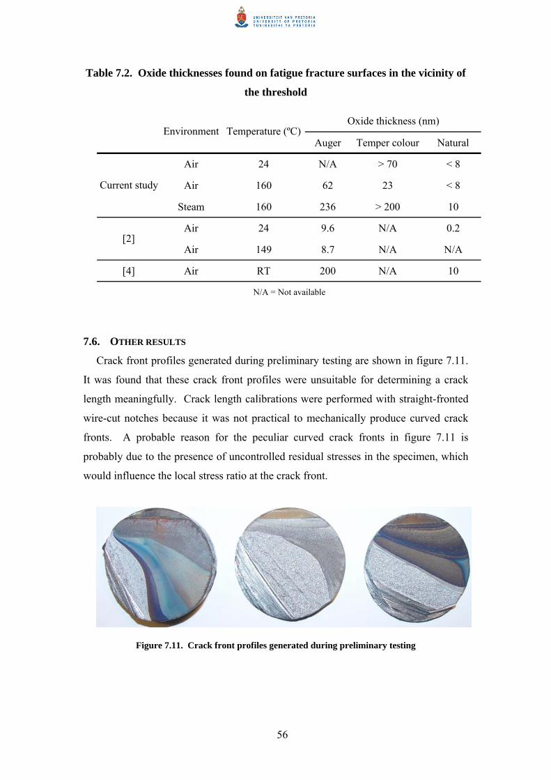
56

Table 7.2. Oxide thicknesses found on fatigue fracture surfaces in the vicinity of

the threshold

Auger Temper colour Natural

Air 24 N/A > 70 < 8

Air 160 62 23 < 8

Steam 160 236 > 200 10

Air 24 9.6 N/A 0.2

Air 149 8.7 N/A N/A

[4] Air RT 200 N/A 10

[2]

Temperature (ºC)Environment

N/A = Not available

Oxide thickness (nm)

Current study

7.6. OTHER RESULTS

Crack front profiles generated during preliminary testing are shown in figure 7.11.

It was found that these crack front profiles were unsuitable for determining a crack

length meaningfully. Crack length calibrations were performed with straight-fronted

wire-cut notches because it was not practical to mechanically produce curved crack

fronts. A probable reason for the peculiar curved crack fronts in figure 7.11 is

probably due to the presence of uncontrolled residual stresses in the specimen, which

would influence the local stress ratio at the crack front.

Figure 7.11. Crack front profiles generated during preliminary testing

57

8. DISCUSSION

8.1. MACHINE DESIGN

From the results it is clear that the custom-built fatigue testing machine simulated

rotating bending successfully. The fracture surfaces that were generated are

reasonably flat transverse to the direction of the maximum cyclically applied principal

stress. From figures 7.2 – 7.4 it is clear that the crack front is symmetrically curved

with respect to the starter notch, indicating that the crack front at the centre grew

faster than the crack front near the surface. The slower growth at the edges may be

due to plane stress conditions at the specimen surface as opposed to plane strain

conditions at the centre of the crack front.

The fact that there is little scatter in the values of the crack growth rate curves

generated is indicative of the reproducibility with which experiments were conducted.

The AC potential drop crack measurement technique employed also correlated well

with the optically measured crack lengths in the vicinity of the threshold.

The straight-line relationship in the Paris region for high stress intensities is given

by mKAdNda

∆= , where m is the slope of the fatigue crack growth rate curve. The

experimental values were obtained at relatively low crack propagation rates, and from

these experiments it was not possible to determine values for m.

The crack faces do not exhibit a “factory rooftop” appearance which would be

expected in the presence of a large shear mode loading. This is due to the fact that

was no fixed torque component was applied to the specimen and the fact that the

cyclic shear stress was only 1/60 of the bending stress (see appendix 11.4).

58

8.2. THE EFFECT OF TEMPERATURE

In a previous study as well as the present study have shown that the threshold

stress intensity value in air decreases as the temperature is increased from 24 °C to

160 °C. The decrease in the threshold value was attributed (Liaw, 1985) to a rougher

fracture surface at the lower temperature, while at the higher temperature the

roughness of the fracture surface was reduced, resulting in less crack closure. The

oxide thicknesses on the fracture surfaces, however, were of the same order (see

figure 4.6). An alternative explanation (Kobayashi, 1991) attributed the decrease in

the threshold value with increasing temperature to the characteristics of the oxide,

ranging from large oxide particles in the crack wake at room temperature to the

formation of only a thin oxide layer at 150 °C (see figure 4.7).

The first explanation is supported by the current observations of intergranular

fracture facets in the vicinity of the threshold for fatigue in air at 24 °C (figure 7.8 and

figure 7.5) and an essentially transgranular fracture surface for fatigue in air at 160 °C

(figure 7.9 and figure 7.6). The current experiments, however, also indicate a

difference in oxide thicknesses. In air at 24 °C the oxide thickness of the dark grey

band was found to be > 70 nm, whereas the thickness of the blue oxide in air at 160

°C was found to be 23 nm. These thicknesses were estimated using the temper colour

scale (Beranger et al, 1996). With the Ar+ sputtering technique employed during

Auger spectroscopy, the blue oxide was found to be nm60~ , but the thickness of the

dark grey oxide of the sample tested in air at 24 °C could not be determined

meaningfully using this technique. This may be due to the fact that the ion sputtering

technique is sensitive to surface roughness.

During normal oxidation at 24 °C and 160 °C without fatigue, the oxide thickness

was previously measured to be < 8 nm (Suresh & Ritchie, 1983). The thicker oxide

layer that developed, especially in the vicinity of the threshold, is probably due to

fretting oxidation. Fretting oxidation (Benoit et al, 1980) is the process whereby the

oxide layer is repeatedly ruptured by relative motion between the mating fracture

surfaces to expose new metal surfaces to be reoxidised. This process leads to the

creation of an excessively thick oxide layer compared with that of a metal surface

naturally oxidised for the same period of time in the same environment. This is

illustrated schematically in figure 8.1.

59

Figure 8.1. Schematic illustration of fretting oxidation compared with natural oxidation

The fracture surfaces produced at 24 °C and 160 °C had similar relative amounts of

α-Fe2O3 and Fe3O4, which is indicative of the same oxidation process. In a number of

studies (Smith, 1987 and Suresh & Ritchie, 1983) it was found that the threshold

value is higher in the wet and moist environments than in dry environments. The

increase in the threshold stress intensity value for moist environments was attributed

to fretting oxidation.

From the above it is concluded that the temperature effect on the threshold value

can be ascribed to roughness-induced crack closure due to the reduction in surface

roughness as the temperature is increased from 24 °C to 160 °C. Oxide-induced crack

closure is of main importance, since the thickening of the oxide layer in the vicinity of

the threshold due to fretting oxidation seems to contribute mostly to the increase of

the threshold value at 24 °C relative to that of air at 160 °C.

60

8.3. THE EFFECT OF THE ENVIRONMENT

In previous studies as well as the present study it was found that the threshold

value increases as the environment is changed from air at 160 °C to steam at 160 °C.

A study in steam and air at 260 °C (Tu & Seth, 1978) found branching cracks

extending over several grains in transverse sections of the specimens tested in steam.

These branching cracks were not only present in the vicinity of the threshold, but also

in regions of higher stress intensities. A dark oxide layer was also found on the

fracture surfaces. This oxide was not identified, neither was the oxide thickness

measured. Branching fatigue cracks were also found for a stainless steel tested in an

argon atmosphere (Keleştemur & Chaki, 2001). In the current study no crack

branching was observed in the transverse section of the specimen tested in steam

(figure 7.7).

In steam the oxide that formed on the fracture surface consisted mainly of Fe3O4,

while a mixture of oxides formed in air. Fe3O4 was also found on fatigue fracture

surfaces of a 508-2 steel in a light water reactor (LWR) environment at 149 °C

(Cullen et al, 1983).

Inspection of figure 7.1 shows that there is an order of magnitude drop in the crack

growth rate in steam at higher stress intensities compared with air at the same stress

intensities. This can be explained by the fact that the black oxide (magnetite) formed

uniformly over the whole fracture surface, from the starter notch to the threshold

(figure 7.4). This is possibly due to the faster oxidation kinetics in a steam

atmosphere during fatigue as well as the contribution of fretting oxidation. The

resulting crack closure effect is therefore probably not only applicable at the threshold

stress intensity level, but is also operative at higher cyclic stress intensities, resulting

in lower crack propagation rates.

61

9. CONCLUSIONS The following conclusions were reached:

• The custom-built fatigue testing machine to simulate rotating bending

operated successfully.

• Fretting oxidation plays a major part in the thickening of oxide layers

during fatigue at near-threshold crack growth rates for the environments

and temperatures investigated.

• The decrease in the threshold value as temperature is increased from 24 °C

to 160 °C is related to the decrease in the oxide thickness and the decrease

in fracture surface roughness.

• Oxide-induced crack closure is probably responsible for the higher

threshold value in steam at 160 °C as opposed to air at 160 °C. It is

deduced that the oxidation kinetics in steam, during fatigue, is fast enough

to also retard the fatigue crack growth rate at higher stress intensities near

the threshold.

62

10. REFERENCES ASTM 647-99.

Benoit D, Namdar-Irani R & Tixier R. 1980. Oxidation of fatigue fracture surfaces at

low crack growth rates. Materials Science and Engineering, Vol. 45, pp 1-7.

Beranger G, Henry G & Sanz G (eds.). 1996. The book of steel. Intercept, p 579.

Bignonnet A, Namdar-Irani R & Truchon M. 1982. The influence of test frequency

on fatigue crack growth in air, and crack surface oxide formation. Scipta

Metallurgica, Vol. 16, pp 795-798.

Carlson RL & Kardomateas GA. 1994. Effects of compressive load excursions on

fatigue crack growth. Fatigue, Vol. 16, February, pp 141-146.

Carpinteri A. 1992. Stress intensity factors for straight-fronted edge cracks in round

bars. Engineering Fracture Mechanics. Vol. 42, No. 6, pp 1035-1040.

Cullen WH, Torronen K & Kemppainen M. 1983. Effect of temperature on fatigue

crack growth of a 508-2 steel in LWR environment. NTIS Technical Report,

Springfield, VA (USA).

Czyryca J. 1985. Fatigue crack initiation. Metals Handbook 9th ed. Vol.8, pp 169-

170.

Geary W & King JE. 1987. Residual stress effects during near-threshold fatigue

crack growth. International Journal of Fatigue. Vol. 9, No. 1, pp 11-16.

Hertzberg RW. 1995. Deformation and fracture mechanics of engineering materials.

Wiley, New York, Chapter12-13, pp 512-698.

Keleştemur MH & Chaki TK. 2001. The effect of various atmospheres on the

threshold fatigue crack growth behaviour of AISI 304 stainless steel. International

Journal of Fatigue. Vol. 23, pp 169-174.

Kemper H, Weiss B & Stricker R. 1989. An alternative presentation of the effects of

the stress-ratio on the fatigue threshold. Engineering Fracture Mechanics, Vol. 32,

No. 4, pp 591-600.

Kobayashi H, Tsuji H & Park KD. 1991. Effect of crack surface oxidation on near-

threshold fatigue crack growth characteristics in A508-3 steel at elevated

temperature. Fracture and Strength ’90, Vol. 51-52, pp 355-360.

Lawson L, Chen EY & Meshii M. 1999. Near-threshold fatigue: a review.

International Journal of Fatigue, Vol. 21, pp S15-S34.

63

Liaw PK. 1985. Mechanisms of near-threshold fatigue crack growth in a low alloy

steel. Acta Metallurgica, Vol. 33, No. 8, pp 1489-1502.

Lindley TC. 1981. Near-threshold fatigue crack growth: experimental methods,

mechanisms and applications. Subcritical crack growth due to fatigue, stress

corrosion and creep – Advanced seminar on fracture mechanics, Italy. Elsevier

Science Publishing, London, pp 167-213.

Lindley TC. 1997. Fretting fatigue in engineering alloys. International Journal of

Fatigue, Vol 19, Supp No 1, pp S39-S49.

Masounave J & Bailon JP. 1976. Effect of grain size on the threshold stress intensity

factor in fatigue of a ferritic steel. Scripta Metallurgica. Vol. 10, pp 165-170.

Schütz W. 1996. A history of fatigue. Engineering Fracture Mechanics, Vol. 54,

No. 2, pp 263-300.

Smith P. 1987. The effect of moisture in the fatigue crack growth behaviour of a low

alloy steel near threshold. Fatigue and Fracture of Engineering Materials and

Structures, Vol. 10, No. 4, pp 291-304.

Suresh S & Ritchie RO. 1983. On the influence of environment on the load ratio

dependence of fatigue thresholds in pressure vessel steel. Engineering Fracture

Mechanics, Vol. 18, No. 4, pp 785-800.

Taylor D. 1988. Fatigue thresholds: their applicability to engineering situations.

International Journal of Fatigue, Vol. 10, No. 2, pp 67-79.

Topper TH & Yu MT. 1985. The effect of overloads on threshold and crack closure.

International Journal of Fatigue, Vol. 7, No. 3, pp 159-164.

Tu LKL & Seth BB. 1978. Threshold corrosion fatigue crack growth in steels.

Journal of Testing and Evaluation, Vol. 6, No. 1, pp 66-74.

Zaiken E & Ritchie RO. 1985. On the role of compression overloads in influencing

crack closure and the threshold condition for fatigue crack growth in 7150

aluminium alloy. Engineering Fracture Mechanics, Vol. 22, No. 1, pp 35-48.

64

11. APPENDIX

11.1. CRACK GROWTH RATE VS. STRESS INTENSITY DATA

Table 11.1. Data for the 24 °C air plot

K∆

( mMPa ) 10.47 9.45 8.93 8.44 8.01 7.57

dNda

(Cyclemm )

5101.1 −× 6107 −× 6103.4 −× 6106.2 −× 7108.8 −× 810−<

Table 11.2. Data for the 160 °C air plot

K∆

( mMPa ) 9.5 8.9 8.1 7.25 6.51 5.87

dNda (

Cyclemm ) 6106.7 −× 6109.3 −× 6105.1 −× 6102.1 −× 7109.7 −× 7104.2 −×

K∆

( mMPa ) 5.6 5.35 4.82

dNda (

Cyclemm ) 7105.1 −× 7109.1 −× 810−<

Table 11.3. Data for the 160 °C steam plot

K∆

( mMPa ) 10 9.5 9 8.5 8 7.5

dNda

(Cyclemm )

7102.9 −× 7106.6 −× 7102.4 −× 7107.2 −× 7103.1 −× 810−<

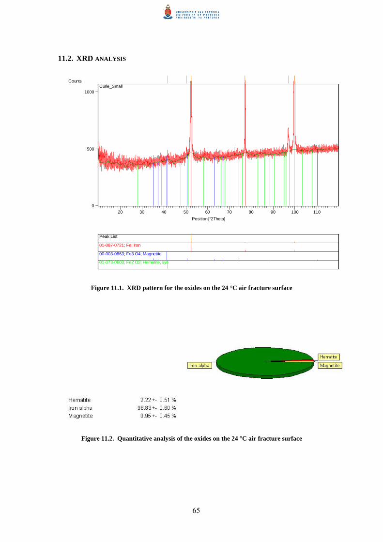
65

11.2. XRD ANALYSIS

Position [°2Theta]20 30 40 50 60 70 80 90 100 110

Counts

0

500

1000 Curle_Small

Peak List

01-087-0721; Fe; Iron

00-003-0863; Fe3 O4; Magnetite

01-073-0603; Fe2 O3; Hematite, syn

Figure 11.1. XRD pattern for the oxides on the 24 °C air fracture surface

Figure 11.2. Quantitative analysis of the oxides on the 24 °C air fracture surface

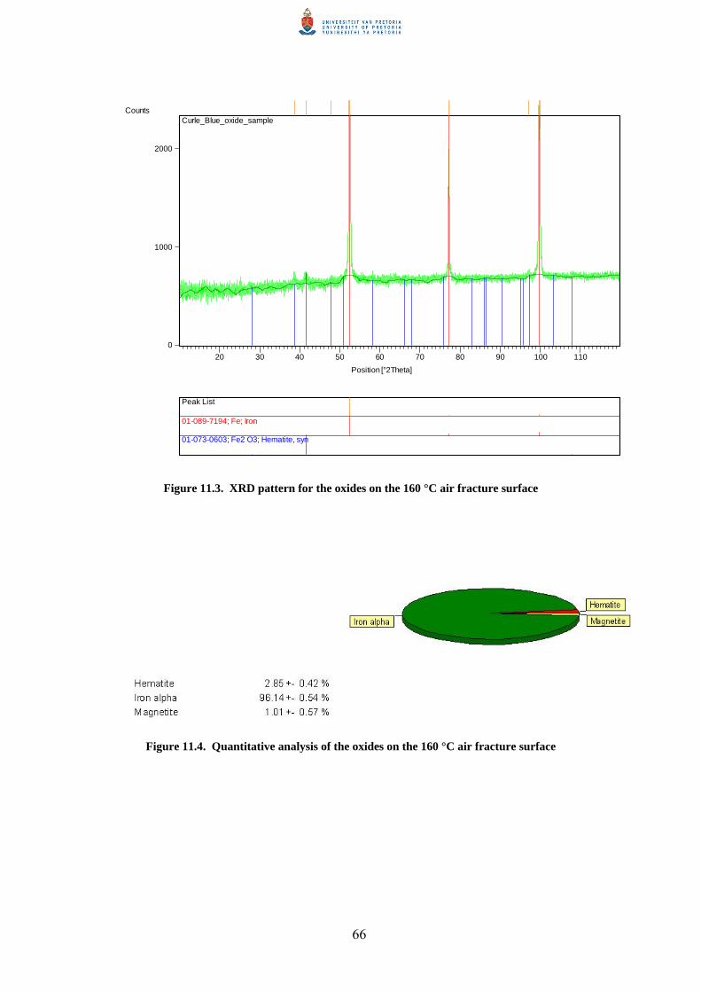
66

Position [°2Theta]20 30 40 50 60 70 80 90 100 110

Counts

0

1000

2000

Curle_Blue_oxide_sample

Peak List

01-089-7194; Fe; Iron

01-073-0603; Fe2 O3; Hematite, syn

Figure 11.3. XRD pattern for the oxides on the 160 °C air fracture surface

Figure 11.4. Quantitative analysis of the oxides on the 160 °C air fracture surface

67

Position [°2Theta]20 30 40 50 60 70 80 90 100 110

Counts

0

500

1000

1500 Curle_Large

Peak List

01-086-1358; Fe2.929 O4; Magnetite

01-087-0721; Fe; Iron

Figure 11.5. XRD pattern for the oxides on the 160 °C steam fracture surface

Figure 11.6. Quantitative analysis of the oxides on the 160 °C steam fracture surface

68

11.3. AUGER SPECTROSCOPY AND SEM ANALYSIS

11.3.1. Auger setting

Survey Analyses: Beam current = 6101 −× A

Beam voltage = 3 kV

Tilt angle = 30º

Depth Profile: Raster size = 11× mm

Ion gun voltage =3 kV

Filament Current = 25 mA

Argon pressure = 31025 −× Pa

Vacuum = 8107 −×

11.3.2. Auger results

Kinetic Energy (eV)

dN(E)

Min: -4678 Max: 4854

50 150 250 350 450 550 650 750 850 950 1050

S1

Fe3

Fe2Fe1

O1

C1

Figure 11.7. Surface spectra for the 24 °C air fracture surface

69

Time (mins.)

N(E)

Min: 20028 Max: 38197

00 2 4 6 8 10 12 14 16 18

Fe3

O1

Fe3

O1

Fe3

O1

Figure 11.8. Typical depth profile of the oxide that formed near the threshold in air at 24 °C

Kinetic Energy (eV)

dN(E)

Min: -4350 Max: 4337

50 150 250 350 450 550 650 750 850 950 1050

Ca1S1

Fe3Fe2

Fe1

O1

C1

Figure 11.9. Surface spectra for the 160 °C air fracture surface

70

Time (mins.)

N(E)

Min: 16065 Max: 41807

00 1 2 3 4 5

Fe3

O1

Fe3

O1

Fe3

O1

Figure 11.10. Depth profile of the oxide that formed near the threshold in air at 160 °C

Kinetic Energy (eV)

dN(E)

Min: -3702 Max: 3711

50 150 250 350 450 550 650 750 850 950 1050

Fe3Fe2Fe1

O1

C1

Cl1S1

Figure 11.11. Surface spectra for the 160 °C steam fracture surface

71

Time (mins.)

N(E)

Min: 15769 Max: 37434

00 2 4 6 8 10 12

Fe3

O1

Fe3

O1

Fe3

O1

Figure 11.12. Depth profile of the oxide that formed near the threshold in steam at 160 °C

Kinetic Energy (eV)

dN(E)

Min: -1873 Max: 1987

50 240 430 620 810 1000 1190 1380 1570 1760 1950

Ta2

O1

C1Ta1

Figure 11.13. Surface spectra for a 1000 Å tantalum oxide standard

72

Time (mins.)

N(E)

Min: 10000 Max: 59450

00 1 2 3 4 5 6 7

O1

Ta1

O1

Ta1

O1

Ta1

Figure 11.14. Depth profile for a 1000 Å tantalum oxide standard

Sputtering rate for 11× mm raster size = 22.5 nm / min

11.3.3. The temper colour scale

Table 11.4. Temper colours as a function of oxide thickness (The book of steel,

1996)

73

11.4. CALCULATION OF THE SHEAR STRESS TO BENDING STRESS RATIO

ZlFMB b ⋅=⋅= σ.. (1)

3

32dZ ⋅=

π (2)

Substitute (2) into (1):

3

.32d

lFb ⋅=∴

πσ (3)

And with

2max8.2

dF

ave ⋅==π

ττ (4)

Divide (4) by (3):

ld

b

⋅=41max

στ

(5)

Substitution with 750=l mm and 50=d mm (from detailed drawing in Section

5.2.2)

601max =∴

bστ

(6)