NCAT Report 14-05 FIELD AND LABORATORY STUDY OF...
114
NCAT Report 14-05 FIELD AND LABORATORY STUDY OF TRINIDAD LAKE ASPHALT MIXTURES AT THE NCAT TEST TRACK By Dr. David H. Timm Dr. Mary M. Robbins Dr. J. Richard Willis Dr. Nam Tran Adam J. Taylor June 17, 2014
Transcript of NCAT Report 14-05 FIELD AND LABORATORY STUDY OF...
NCAT Report 14-05
FIELD AND LABORATORY STUDY OF TRINIDAD LAKE ASPHALT MIXTURES
AT THE NCAT TEST TRACK
By Dr. David H. Timm
Dr. Mary M. Robbins Dr. J. Richard Willis
Dr. Nam Tran Adam J. Taylor
June 17, 2014
i
FIELD AND LABORATORY STUDY OF TRINIDAD LAKE ASPHALT MIXTURES AT THE NCAT TEST TRACK
By Dr. David H. Timm
Dr. Mary M. Robbins Dr. J. Richard Willis
Dr. Nam Tran Adam J. Taylor
National Center for Asphalt Technology Auburn University
Sponsored by Lake Asphalt of Trinidad and Tobago (1978) Ltd
June 17, 2014
ii
ACKNOWLEDGEMENTS This project was sponsored by Lake Asphalt of Trinidad and Tobago (1978) Ltd. Deonarine Sarabjit of Lake Asphalt of Trinidad and Tobago (1978) Ltd deserves special recognition for providing detailed technical and editorial review of this document.
DISCLAIMER The contents of this report reflect the views of the authors who are responsible for the facts and accuracy of the data presented herein. The contents do not necessarily reflect the official views or policies of Lake Asphalt of Trinidad and Tobago (1978) Ltd or the National Center for Asphalt Technology, or Auburn University. This report does not constitute a standard, specification, or regulation. Comments contained in this paper related to specific testing equipment and materials should not be considered an endorsement of any commercial product or service; no such endorsement is intended or implied.
Timm, Robbins, Willis, Tran, Taylor
i
TABLE OF CONTENTS
1. INTRODUCTION .....................................................................................................................1
1.1. Background ......................................................................................................................1 1.2. Objectives and Scope of Work ..........................................................................................1
2. INSTRUMENTATION .............................................................................................................2 3. MIX DESIGN, CONSTRUCTION AND INSTRUMENTATION INSTALLATION ............3
3.1. Mix Design ......................................................................................................................4 3.2. Construction and Instrumentation Installation ...................................................................5
4. LABORATORY TESTING ON BINDERS AND PLANT PRODUCED MIXTURES ........18 4.1. Compaction of Performance Testing Specimens from Plant-Produced Mixes ...............18 4.2. Binder Properties .............................................................................................................19
4.2.1. Performance Grades According to AASHTO M 320-10 .......................................19 4.2.2. Performance Grade using MSCR According to AASHTO M 19-10 ....................19
4.3. Dynamic Modulus Testing ...............................................................................................20 4.4. Beam Fatigue Testing ......................................................................................................28 4.5. Simplified Visco-elastic Continuum Damage .................................................................32 4.6. Asphalt Pavement Analyzer (APA) Testing ....................................................................34 4.7. Flow Number Testing ......................................................................................................36 4.8. Energy Ratio Testing .......................................................................................................37 4.9. Indirect Tension Creep Compliance and Strength ...........................................................38 4.10. Hamburg Wheel Tracking Test .......................................................................................41 4.11. Moisture Damage ............................................................................................................44
5. FALLING WEIGHT DEFLECTOMETER TESTING AND BACKCALCULATION .........45 6. PAVEMENT RESPONSE MEASUREMENTS .....................................................................51
6.1. Seasonal Trends in Pavement Response ..........................................................................54 6.2. Pavement Response vs. Temperature ..............................................................................57 6.3. Pavement Responses Normalized to Reference Temperatures ........................................60
6.3.1. Longitudinal Strain Responses ..............................................................................60 6.3.2. Transverse Strain Responses ..................................................................................61 6.3.3. Aggregate Base Vertical Pressure Responses ........................................................62 6.3.4. Subgrade Vertical Pressure Responses ..................................................................63
6.4. Pavement Response Over Time at 68°F ..........................................................................64 7. PAVEMENT PERFORMANCE .............................................................................................67 8. KEY FINDINGS, CONCLUSIONS AND RECOMMENDATIONS ....................................71
8.1. Laboratory Characterization ............................................................................................71 8.2. Construction ....................................................................................................................72 8.3. Structural Response Characterization ..............................................................................72 8.4. Field Performance ............................................................................................................73
REFERENCES ....................................................................................................................74 APPENDIX A – MIX DESIGN AND AS BUILT AC PROPERTIES .........................................77 APPENDIX B – SURVEYED PAVEMENT DEPTHS ................................................................84 APPENDIX C – BINDER GRADING ..........................................................................................86 APPENDIX D – MASTER CURVE DATA .................................................................................95 APPENDIX E – IDT CREEP COMPLIANCE DATA ...............................................................106
Timm, Robbins, Willis, Tran, Taylor
ii
LIST OF TABLES
Table 3.1 Mix Design Gradations – Percent Passing Sieve Sizes ...................................................4 Table 3.2 Mix Design Parameters ....................................................................................................5 Table 3.3 Random Locations ...........................................................................................................6 Table 3.4 Subgrade Dry Unit Weight and Moisture Contents .........................................................7 Table 3.5 Aggregate Base Dry Unit Weight and Moisture Contents ..............................................9 Table 3.6 Date of Paving ...............................................................................................................12 Table 3.7 Material Inventory for Laboratory Testing ....................................................................12 Table 3.8 Asphalt Concrete Layer Properties – As Built ...............................................................14 Table 4.1 Summary of Gmm and Laboratory Compaction Temperatures ......................................18 Table 4.2 Grading of Binders .........................................................................................................19 Table 4.3 Non-Recoverable Creep Compliance at Multiple Stress Levels ...................................20 Table 4.4 Requirements for Non-Recoverable Creep Compliance (AASHTO MP 19-10) ..........20 Table 4.5 Production Tolerances for Dynamic Modulus and Flow Number Specimens (AASHTO PP 60-09) .......................................................................................................................................21 Table 4.6 Temperatures and Frequencies used for Dynamic Modulus Testing ............................22 Table 4.7 High Test Temperature for Dynamic Modulus Testing .................................................22 Table 4.8 Dynamic Modulus Data Quality Threshold Values .......................................................22 Table 4.9 Master Curve Equation Variable Descriptions ..............................................................24 Table 4.10 Master Curve Coefficients – Unconfined ....................................................................25 Table 4.11 Master Curve Coefficients – 20 psi Confinement .......................................................25 Table 4.12 Bending Beam Fatigue Results ....................................................................................30 Table 4.13 Fatigue Curve Fitting Coefficients (Power Model Form) ...........................................31 Table 4.14 Percent Increase in Cycles to Failure for TLA versus Control Mixture ......................32 Table 4.15 Predicted Endurance Limits .........................................................................................32 Table 4.16 APA Test Results .........................................................................................................34 Table 4.17 Flow Number Criteria from NCHRP 09-33 (HMA) (Bonaquist, 2011) and 09-43 (WMA) (Bonaquist, 2011) .............................................................................................................36 Table 4.18 Energy Ratio Test Results ............................................................................................38 Table 4.19 Average Measured IDT Strength Data at -10°C (MPa) ...............................................39 Table 4.20 Failure Time and Critical Temperature .......................................................................41 Table 4.21 Tukey-Kramer Results – Rutting Results ....................................................................44 Table 4.22 Summary of TSR Testing ............................................................................................45 Table 5.1 FWD Sensor Spacing .....................................................................................................46 Table 5.2 FWD Drop Heights and Approximate Weights .............................................................46 Table 6.1 Pavement Response vs. Temperature Regression Terms ..............................................60 Table 6.2 Predicted Fatigue Life at 68°F .......................................................................................61
Timm, Robbins, Willis, Tran, Taylor
iii
LIST OF FIGURES
Figure 1.1 TLA Pellets .....................................................................................................................1 Figure 2.1 Gauge Array ...................................................................................................................3 Figure 3.1 Cross-Section Design: Materials and Lift Thicknesses ..................................................3 Figure 3.2 Random Location and Instrumentation Schematic .........................................................6 Figure 3.3 Subgrade Earth Pressure Cell Installation Prior to Final Covering ................................7 Figure 3.4 Final Survey of Subgrade Earth Pressure Cell ...............................................................7 Figure 3.5 Subgrade and Aggregate Base ........................................................................................8 Figure 3.6 Surveyed Aggregate Base Thickness .............................................................................9 Figure 3.7 Gauge Installation: (a) Preparing grid and laying out gauges; (b) Trench preparation; (c) Gauges placed for paving; (d) Placing protective cover material over each gauge; (e) Paving over gauges ....................................................................................................................................10 Figure 3.8 TLA Pellets Fed Through RAP Feed System During Track Mix Production ..............11 Figure 3.9 Mixture Sampling for Lab Testing ...............................................................................13 Figure 3.10 S12 (TLA) Measured and Predicted Cooling Curves (Lifts 1, 2 and 3) .....................15 Figure 3.11 S9 (Control) Measured and Predicted Cooling Curves (Lifts 1, 2 and 3) ..................15 Figure 3.12 Average Lift Thicknesses and Depth of Instrumentation ...........................................16 Figure 3.13 Temperature Probe Installation ..................................................................................17 Figure 3.14 Asphalt Strain Gauge Survivability ............................................................................17 Figure 4.1 IPC Global Asphalt Mixture Performance Tester ........................................................21 Figure 4.2 Example Master Curve Generation ..............................................................................23 Figure 4.3 Dynamic Modulus Master Curves – Surface Mixes – Unconfined ..............................26 Figure 4.4 Dynamic Modulus Master Curves – Surface Mixes – Confined (20 psi) ....................26 Figure 4.5 Dynamic Modulus Master Curves – Intermediate and Base Mixes – Unconfined ......27 Figure 4.6 Dynamic Modulus Master Curves – Intermediate and Base Mixes – Confined (20 psi) ........................................................................................................................27 Figure 4.7 Kneading Beam Compactor .........................................................................................28 Figure 4.8 IPC Global Beam Fatigue Testing Apparatus ..............................................................29 Figure 4.9 Comparison of Fatigue Resistance for Mixtures ..........................................................31 Figure 4.10 C vs. S Curve ..............................................................................................................33 Figure 4.11 Predicted Cycles to Failure .........................................................................................33 Figure 4.12 Asphalt Pavement Analyzer .......................................................................................34 Figure 4.13 Rate of Rutting Plot ....................................................................................................35 Figure 4.14 Flow Number Test Results .........................................................................................37 Figure 4.15 Predicted Thermal Stress versus Temperature ...........................................................41 Figure 4.16 Hamburg Wheel-Tracking Device .............................................................................42 Figure 4.17 Example Hamburg Raw Data Output .........................................................................42 Figure 4.18 SIP from HWTT .........................................................................................................43 Figure 4.19 Rutting Results from HWTT ......................................................................................44
Timm, Robbins, Willis, Tran, Taylor
iv
Figure 5.1 Dynatest Model 8000 FWD ..........................................................................................46 Figure 5.2 Backcalculated AC Modulus vs. Date (Section-Wide Average) ..................................47 Figure 5.3 Backcalculated Granular Base Modulus vs. Date (Section-Wide Average) ................48 Figure 5.4 Backcalculated Subgrade Soil Modulus vs. Date (Section-Wide Average) .................48 Figure 5.5 Backcalculated AC Modulus vs. Mid-Depth Temperature (RMSE<3%) ....................49 Figure 5.6 Backcalculated AC Modulus Corrected to Reference Temperatures ...........................50 Figure 5.7 Backcalculated AC Modulus vs. Date at 68°F .............................................................51 Figure 6.1 DaDISP Screen Capture of Pressure Measurements for Truck Pass ............................52 Figure 6.2 DaDISP Screen Capture of Longitudinal Strain Measurements ..................................53 Figure 6.3 DaDISP Screen Capture of Transverse Strain Measurements .....................................54 Figure 6.4 Longitudinal Microstrain Under Single Axles .............................................................55 Figure 6.5 Transverse Microstrain Under Single Axles ................................................................55 Figure 6.6 Aggregate Base Pressure Under Single Axles ..............................................................56 Figure 6.7 Subgrade Pressure Under Single Axles ........................................................................56 Figure 6.8 Longitudinal Strain vs. Mid-Depth Temperature Under Single Axles .........................58 Figure 6.9 Transverse Strain vs. Mid-Depth Temperature Under Single Axles ............................58 Figure 6.10 Base Pressure vs. Mid-Depth Temperature Under Single Axles ...............................59 Figure 6.11 Subgrade Pressure vs. Mid-Depth Temperature Under Single Axles ........................59 Figure 6.16 Longitudinal Strain Under Single Axles at Three Reference Temperatures ..............61 Figure 6.17 Transverse Strain Under Single Axles at Three Reference Temperatures .................62 Figure 6.18 Base Pressure Under Single Axles at Three Reference Temperatures .......................63 Figure 6.19 Subgrade Pressure Under Single Axles at Three Reference Temperatures ...............64 Figure 6.20 Longitudinal Microstrain Under Single Axles vs. Date at 68°F ................................65 Figure 6.21 Transverse Microstrain Under Single Axles vs. Date at 68°F....................................65 Figure 6.22 Base Pressure Under Single Axles vs. Date at 68°F ..................................................66 Figure 6.23 Subgrade Pressure Under Single Axles vs. Date at 68°F ...........................................66 Figure 7.1 Measured Rut Depths – ARAN ....................................................................................67 Figure 7.2 Measured Rut Depth – Final Wireline..........................................................................68 Figure 7.3 Measured IRI ................................................................................................................69 Figure 7.4 IRI – Left Wheelpath of S12 ........................................................................................69 Figure 7.5 IRI – Right Wheelpath of S12 ......................................................................................70 Figure 7.6 Transition from S11 to S12 ..........................................................................................70
Timm, Robbins, Willis, Tran, Taylor
1
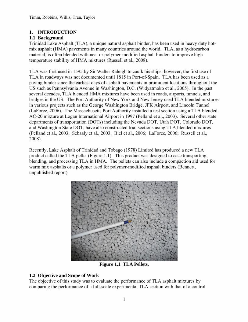
1. INTRODUCTION 1.1 Background Trinidad Lake Asphalt (TLA), a unique natural asphalt binder, has been used in heavy duty hot- mix asphalt (HMA) pavements in many countries around the world. TLA, as a hydrocarbon material, is often blended with neat or polymer-modified asphalt binders to improve high temperature stability of HMA mixtures (Russell et al., 2008). TLA was first used in 1595 by Sir Walter Raleigh to caulk his ships; however, the first use of TLA in roadways was not documented until 1815 in Port-of-Spain. TLA has been used as a paving binder since the earliest days of asphalt pavements in prominent locations throughout the US such as Pennsylvania Avenue in Washington, D.C. (Widyatmoko et al., 2005). In the past several decades, TLA blended HMA mixtures have been used in roads, airports, tunnels, and bridges in the US. The Port Authority of New York and New Jersey used TLA blended mixtures in various projects such as the George Washington Bridge, JFK Airport, and Lincoln Tunnel (LaForce, 2006). The Massachusetts Port Authority installed a test section using a TLA blended AC-20 mixture at Logan International Airport in 1997 (Pelland et al., 2003). Several other state departments of transportation (DOTs) including the Nevada DOT, Utah DOT, Colorado DOT, and Washington State DOT, have also constructed trial sections using TLA blended mixtures (Pelland et al., 2003; Sebaaly et al., 2003; Biel et al., 2006; LaForce, 2006; Russell et al., 2008). Recently, Lake Asphalt of Trinidad and Tobago (1978) Limited has produced a new TLA product called the TLA pellet (Figure 1.1). This product was designed to ease transporting, blending, and processing TLA in HMA. The pellets can also include a compaction aid used for warm mix asphalts or a polymer used for polymer-modified asphalt binders (Bennert, unpublished report).
Figure 1.1 TLA Pellets.
1.2 Objective and Scope of Work The objective of this study was to evaluate the performance of TLA asphalt mixtures by comparing the performance of a full-scale experimental TLA section with that of a control
Timm, Robbins, Willis, Tran, Taylor
2
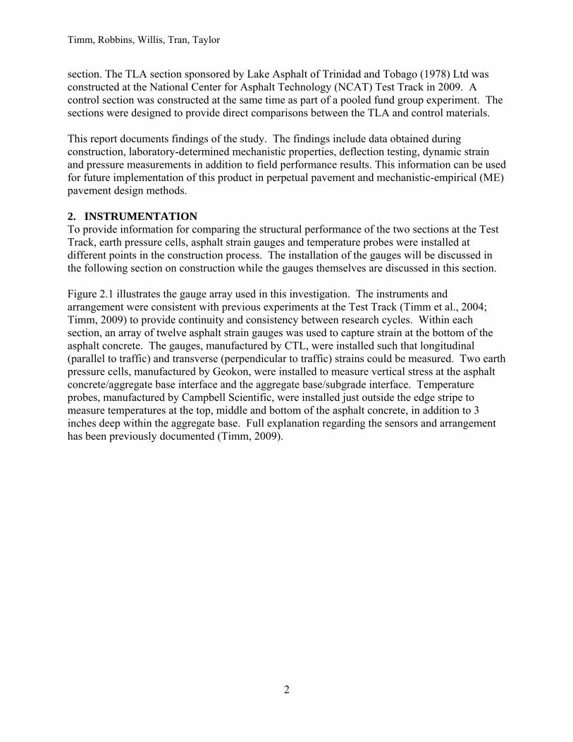
section. The TLA section sponsored by Lake Asphalt of Trinidad and Tobago (1978) Ltd was constructed at the National Center for Asphalt Technology (NCAT) Test Track in 2009. A control section was constructed at the same time as part of a pooled fund group experiment. The sections were designed to provide direct comparisons between the TLA and control materials. This report documents findings of the study. The findings include data obtained during construction, laboratory-determined mechanistic properties, deflection testing, dynamic strain and pressure measurements in addition to field performance results. This information can be used for future implementation of this product in perpetual pavement and mechanistic-empirical (ME) pavement design methods. 2. INSTRUMENTATION To provide information for comparing the structural performance of the two sections at the Test Track, earth pressure cells, asphalt strain gauges and temperature probes were installed at different points in the construction process. The installation of the gauges will be discussed in the following section on construction while the gauges themselves are discussed in this section. Figure 2.1 illustrates the gauge array used in this investigation. The instruments and arrangement were consistent with previous experiments at the Test Track (Timm et al., 2004; Timm, 2009) to provide continuity and consistency between research cycles. Within each section, an array of twelve asphalt strain gauges was used to capture strain at the bottom of the asphalt concrete. The gauges, manufactured by CTL, were installed such that longitudinal (parallel to traffic) and transverse (perpendicular to traffic) strains could be measured. Two earth pressure cells, manufactured by Geokon, were installed to measure vertical stress at the asphalt concrete/aggregate base interface and the aggregate base/subgrade interface. Temperature probes, manufactured by Campbell Scientific, were installed just outside the edge stripe to measure temperatures at the top, middle and bottom of the asphalt concrete, in addition to 3 inches deep within the aggregate base. Full explanation regarding the sensors and arrangement has been previously documented (Timm, 2009).
Timm, Robbins, Willis, Tran, Taylor
3
Figure 2.1 Gauge Array
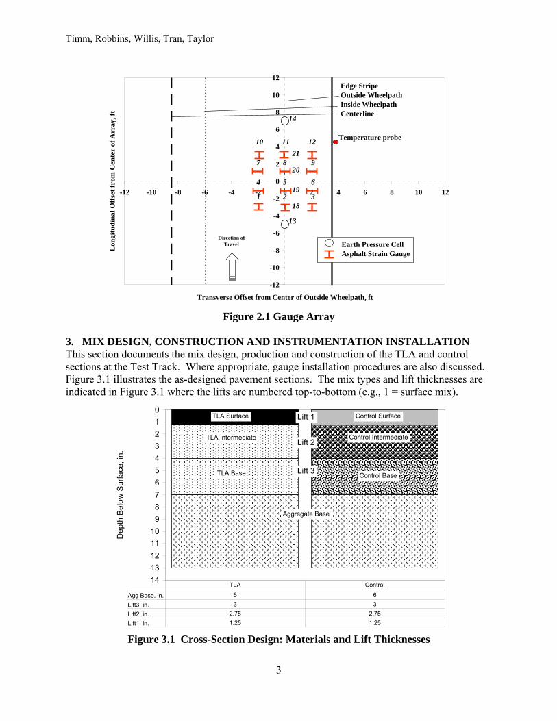
3. MIX DESIGN, CONSTRUCTION AND INSTRUMENTATION INSTALLATION This section documents the mix design, production and construction of the TLA and control sections at the Test Track. Where appropriate, gauge installation procedures are also discussed. Figure 3.1 illustrates the as-designed pavement sections. The mix types and lift thicknesses are indicated in Figure 3.1 where the lifts are numbered top-to-bottom (e.g., 1 = surface mix).
Figure 3.1 Cross-Section Design: Materials and Lift Thicknesses
-12
-10
-8
-6
-4
-2
0
2
4
6
8
10
12
-12 -10 -8 -6 -4 -2 0 2 4 6 8 10 12
Transverse Offset from Center of Outside Wheelpath, ft
Lon
gitu
din
al O
ffse
t fr
om C
ente
r of
Arr
ay, f
t
Earth Pressure CellAsphalt Strain Gauge
Edge StripeOutside WheelpathInside WheelpathCenterline
Direction of Travel
1 2 3
4 5 6
7 8 9
10 11 12
13
14
21
20
19
18
Temperature probe
0
1
2
3
4
5
6
7
8
9
10
11
12
13
14
Dep
th B
elow
Sur
face
, in
.
Agg Base, in. 6 6
Lift3, in. 3 3
Lift2, in. 2.75 2.75
Lift1, in. 1.25 1.25
TLA Control
TLA Intermediate
TLA Surface Control Surface
Control Intermediate
Control Base
Aggregate Base
TLA Base Lift 3
Lift 2
Lift 1
Timm, Robbins, Willis, Tran, Taylor
4
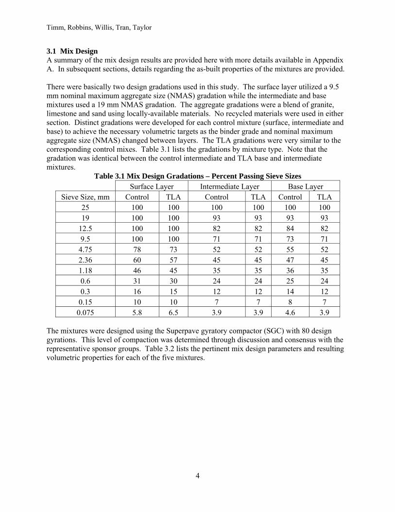
3.1 Mix Design A summary of the mix design results are provided here with more details available in Appendix A. In subsequent sections, details regarding the as-built properties of the mixtures are provided. There were basically two design gradations used in this study. The surface layer utilized a 9.5 mm nominal maximum aggregate size (NMAS) gradation while the intermediate and base mixtures used a 19 mm NMAS gradation. The aggregate gradations were a blend of granite, limestone and sand using locally-available materials. No recycled materials were used in either section. Distinct gradations were developed for each control mixture (surface, intermediate and base) to achieve the necessary volumetric targets as the binder grade and nominal maximum aggregate size (NMAS) changed between layers. The TLA gradations were very similar to the corresponding control mixes. Table 3.1 lists the gradations by mixture type. Note that the gradation was identical between the control intermediate and TLA base and intermediate mixtures.
Table 3.1 Mix Design Gradations – Percent Passing Sieve Sizes Surface Layer Intermediate Layer Base Layer
Sieve Size, mm Control TLA Control TLA Control TLA 25 100 100 100 100 100 100 19 100 100 93 93 93 93
12.5 100 100 82 82 84 82 9.5 100 100 71 71 73 71 4.75 78 73 52 52 55 52 2.36 60 57 45 45 47 45 1.18 46 45 35 35 36 35 0.6 31 30 24 24 25 24 0.3 16 15 12 12 14 12 0.15 10 10 7 7 8 7 0.075 5.8 6.5 3.9 3.9 4.6 3.9
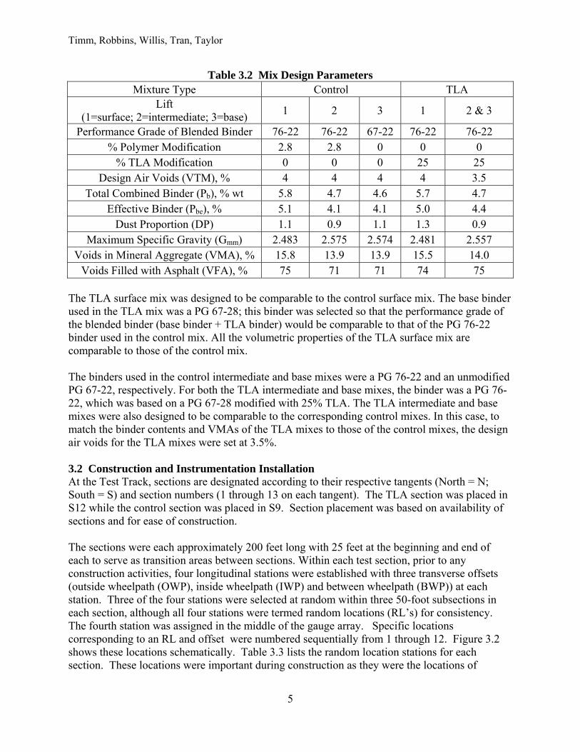
The mixtures were designed using the Superpave gyratory compactor (SGC) with 80 design gyrations. This level of compaction was determined through discussion and consensus with the representative sponsor groups. Table 3.2 lists the pertinent mix design parameters and resulting volumetric properties for each of the five mixtures.
Timm, Robbins, Willis, Tran, Taylor
5
Table 3.2 Mix Design Parameters Mixture Type Control TLA
Lift (1=surface; 2=intermediate; 3=base)
1 2 3 1 2 & 3
Performance Grade of Blended Binder 76-22 76-22 67-22 76-22 76-22 % Polymer Modification 2.8 2.8 0 0 0
% TLA Modification 0 0 0 25 25 Design Air Voids (VTM), % 4 4 4 4 3.5
Total Combined Binder (Pb), % wt 5.8 4.7 4.6 5.7 4.7 Effective Binder (Pbe), % 5.1 4.1 4.1 5.0 4.4
Dust Proportion (DP) 1.1 0.9 1.1 1.3 0.9 Maximum Specific Gravity (Gmm) 2.483 2.575 2.574 2.481 2.557
Voids in Mineral Aggregate (VMA), % 15.8 13.9 13.9 15.5 14.0 Voids Filled with Asphalt (VFA), % 75 71 71 74 75
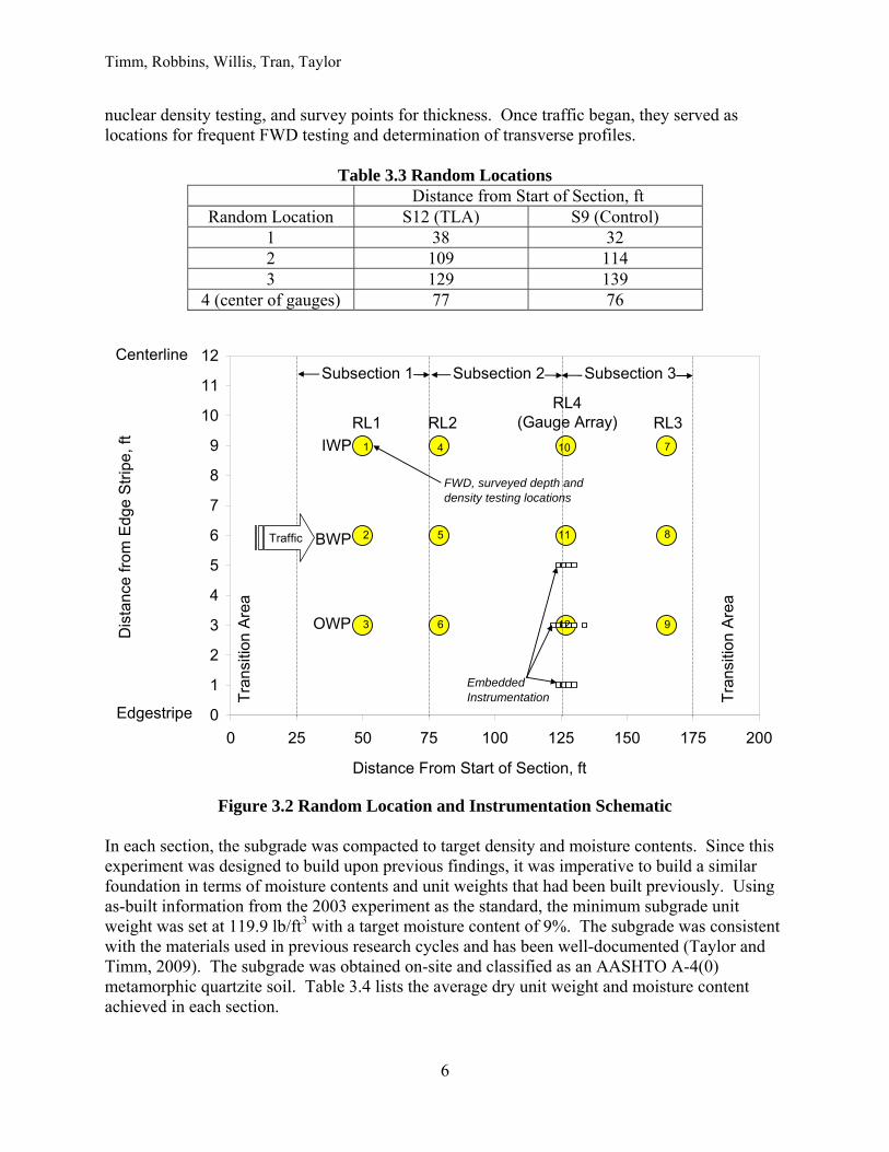
The TLA surface mix was designed to be comparable to the control surface mix. The base binder used in the TLA mix was a PG 67-28; this binder was selected so that the performance grade of the blended binder (base binder + TLA binder) would be comparable to that of the PG 76-22 binder used in the control mix. All the volumetric properties of the TLA surface mix are comparable to those of the control mix. The binders used in the control intermediate and base mixes were a PG 76-22 and an unmodified PG 67-22, respectively. For both the TLA intermediate and base mixes, the binder was a PG 76-22, which was based on a PG 67-28 modified with 25% TLA. The TLA intermediate and base mixes were also designed to be comparable to the corresponding control mixes. In this case, to match the binder contents and VMAs of the TLA mixes to those of the control mixes, the design air voids for the TLA mixes were set at 3.5%. 3.2 Construction and Instrumentation Installation At the Test Track, sections are designated according to their respective tangents (North = N; South = S) and section numbers (1 through 13 on each tangent). The TLA section was placed in S12 while the control section was placed in S9. Section placement was based on availability of sections and for ease of construction. The sections were each approximately 200 feet long with 25 feet at the beginning and end of each to serve as transition areas between sections. Within each test section, prior to any construction activities, four longitudinal stations were established with three transverse offsets (outside wheelpath (OWP), inside wheelpath (IWP) and between wheelpath (BWP)) at each station. Three of the four stations were selected at random within three 50-foot subsections in each section, although all four stations were termed random locations (RL’s) for consistency. The fourth station was assigned in the middle of the gauge array. Specific locations corresponding to an RL and offset were numbered sequentially from 1 through 12. Figure 3.2 shows these locations schematically. Table 3.3 lists the random location stations for each section. These locations were important during construction as they were the locations of
Timm, Robbins, Willis, Tran, Taylor
6
nuclear density testing, and survey points for thickness. Once traffic began, they served as locations for frequent FWD testing and determination of transverse profiles.
Table 3.3 Random Locations
Distance from Start of Section, ft Random Location S12 (TLA) S9 (Control)
1 38 32 2 109 114 3 129 139
4 (center of gauges) 77 76
Figure 3.2 Random Location and Instrumentation Schematic
In each section, the subgrade was compacted to target density and moisture contents. Since this experiment was designed to build upon previous findings, it was imperative to build a similar foundation in terms of moisture contents and unit weights that had been built previously. Using as-built information from the 2003 experiment as the standard, the minimum subgrade unit weight was set at 119.9 lb/ft3 with a target moisture content of 9%. The subgrade was consistent with the materials used in previous research cycles and has been well-documented (Taylor and Timm, 2009). The subgrade was obtained on-site and classified as an AASHTO A-4(0) metamorphic quartzite soil. Table 3.4 lists the average dry unit weight and moisture content achieved in each section.
0
1
2
3
4
5
6
7
8
9
10
11
12
0 25 50 75 100 125 150 175 200
Distance From Start of Section, ft
Dis
tanc
e fr
om E
dge
Str
ipe
, ft
1
2
3
4
5
6
10
11
12
7
8
9
Centerline
Edgestripe
RL1 RL2RL4
(Gauge Array) RL3
IWP
BWP
OWP
FWD, surveyed depth and density testing locations
Subsection 1 Subsection 2 Subsection 3
Tra
nsiti
on A
rea
Tra
nsiti
on A
rea
Traffic
EmbeddedInstrumentation
Timm, Robbins, Willis, Tran, Taylor
7
Table 3.4 Subgrade Dry Unit Weight and Moisture Contents Test Section S12 (TLA) S9 (Control)
Average Dry Unit Weight, lb/ft3 122.6 123.4 Average Moisture Content, % 10.1 9.2
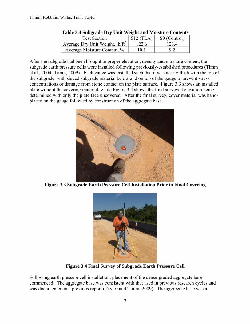
After the subgrade had been brought to proper elevation, density and moisture content, the subgrade earth pressure cells were installed following previously-established procedures (Timm et al., 2004; Timm, 2009). Each gauge was installed such that it was nearly flush with the top of the subgrade, with sieved subgrade material below and on top of the gauge to prevent stress concentrations or damage from stone contact on the plate surface. Figure 3.3 shows an installed plate without the covering material, while Figure 3.4 shows the final surveyed elevation being determined with only the plate face uncovered. After the final survey, cover material was hand-placed on the gauge followed by construction of the aggregate base.
Figure 3.3 Subgrade Earth Pressure Cell Installation Prior to Final Covering
Figure 3.4 Final Survey of Subgrade Earth Pressure Cell
Following earth pressure cell installation, placement of the dense-graded aggregate base commenced. The aggregate base was consistent with that used in previous research cycles and was documented in a previous report (Taylor and Timm, 2009). The aggregate base was a
Timm, Robbins, Willis, Tran, Taylor
8
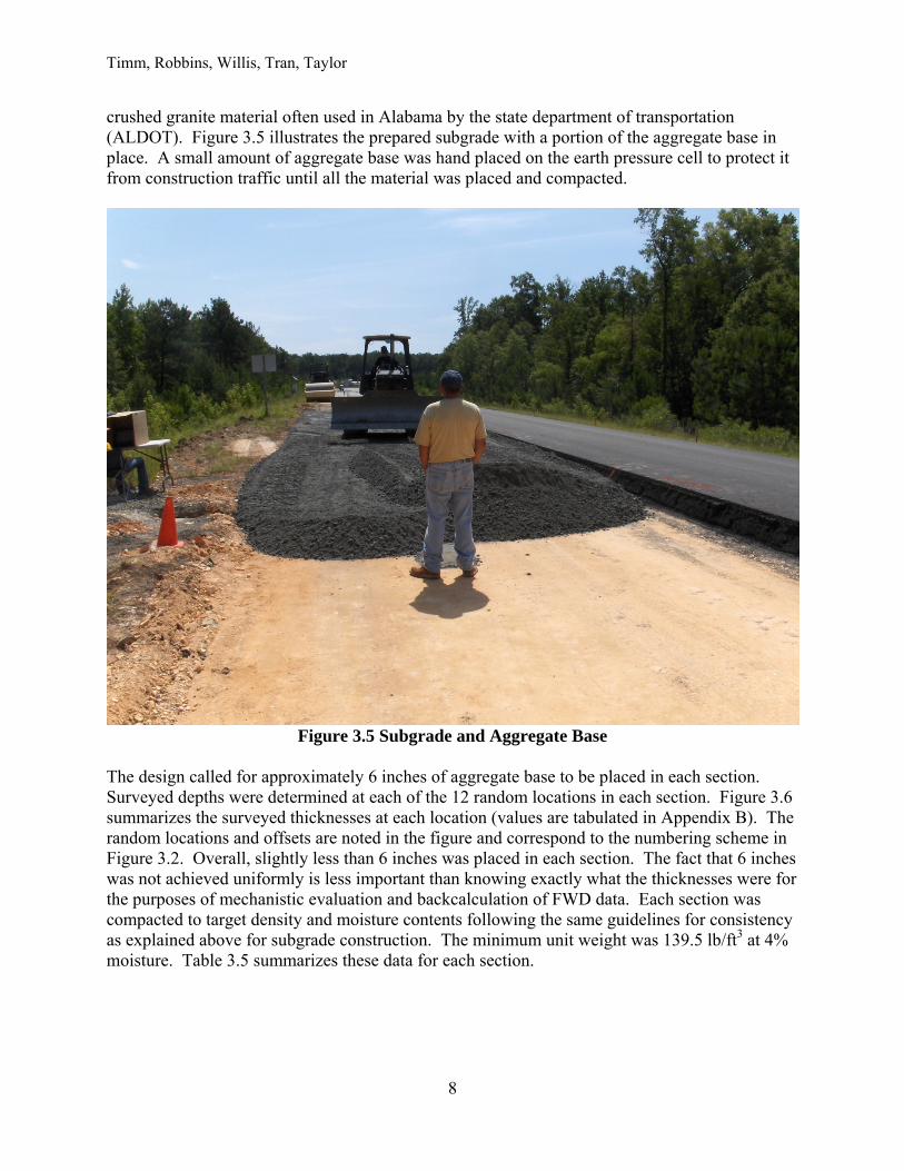
crushed granite material often used in Alabama by the state department of transportation (ALDOT). Figure 3.5 illustrates the prepared subgrade with a portion of the aggregate base in place. A small amount of aggregate base was hand placed on the earth pressure cell to protect it from construction traffic until all the material was placed and compacted.
Figure 3.5 Subgrade and Aggregate Base
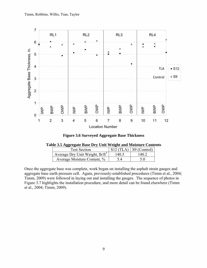
The design called for approximately 6 inches of aggregate base to be placed in each section. Surveyed depths were determined at each of the 12 random locations in each section. Figure 3.6 summarizes the surveyed thicknesses at each location (values are tabulated in Appendix B). The random locations and offsets are noted in the figure and correspond to the numbering scheme in Figure 3.2. Overall, slightly less than 6 inches was placed in each section. The fact that 6 inches was not achieved uniformly is less important than knowing exactly what the thicknesses were for the purposes of mechanistic evaluation and backcalculation of FWD data. Each section was compacted to target density and moisture contents following the same guidelines for consistency as explained above for subgrade construction. The minimum unit weight was 139.5 lb/ft3 at 4% moisture. Table 3.5 summarizes these data for each section.
Timm, Robbins, Willis, Tran, Taylor
9
Figure 3.6 Surveyed Aggregate Base Thickness
Table 3.5 Aggregate Base Dry Unit Weight and Moisture Contents
Test Section S12 (TLA) S9 (Control) Average Dry Unit Weight, lb/ft3 140.5 140.2 Average Moisture Content, % 5.4 5.0
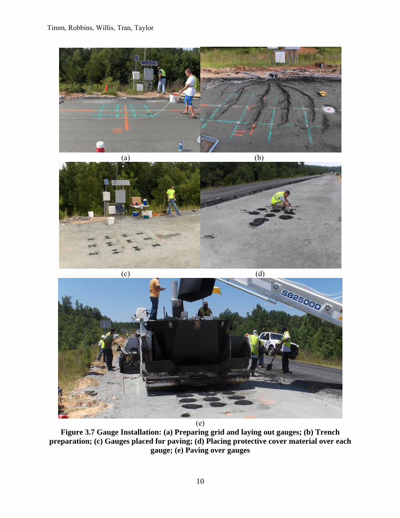
Once the aggregate base was complete, work began on installing the asphalt strain gauges and aggregate base earth pressure cell. Again, previously-established procedures (Timm et al., 2004; Timm, 2009) were followed in laying out and installing the gauges. The sequence of photos in Figure 3.7 highlights the installation procedure, and more detail can be found elsewhere (Timm et al., 2004; Timm, 2009).
0
1
2
3
4
5
6
7
1 2 3 4 5 6 7 8 9 10 11 12
Location Number
Agg
rega
te B
ase
Thi
ckne
ss,
in.
S12
S9
RL1 RL2 RL3 RL4
IWP
BW
P
OW
P
IWP
BW
P
OW
P
IWP
BW
P
OW
P
IWP
BW
P
OW
P
TLA
Control
Timm, Robbins, Willis, Tran, Taylor
10
(a) (b)
(c) (d)
(e)
Figure 3.7 Gauge Installation: (a) Preparing grid and laying out gauges; (b) Trench preparation; (c) Gauges placed for paving; (d) Placing protective cover material over each
gauge; (e) Paving over gauges
Timm, Robbins, Willis, Tran, Taylor
11
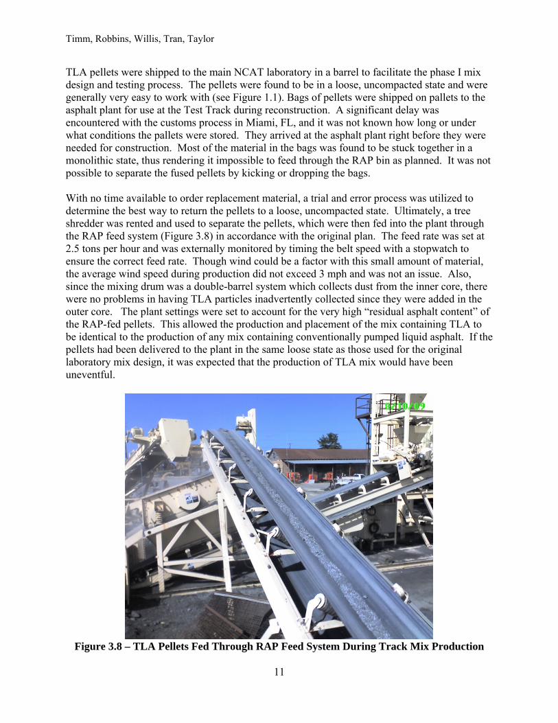
TLA pellets were shipped to the main NCAT laboratory in a barrel to facilitate the phase I mix design and testing process. The pellets were found to be in a loose, uncompacted state and were generally very easy to work with (see Figure 1.1). Bags of pellets were shipped on pallets to the asphalt plant for use at the Test Track during reconstruction. A significant delay was encountered with the customs process in Miami, FL, and it was not known how long or under what conditions the pallets were stored. They arrived at the asphalt plant right before they were needed for construction. Most of the material in the bags was found to be stuck together in a monolithic state, thus rendering it impossible to feed through the RAP bin as planned. It was not possible to separate the fused pellets by kicking or dropping the bags. With no time available to order replacement material, a trial and error process was utilized to determine the best way to return the pellets to a loose, uncompacted state. Ultimately, a tree shredder was rented and used to separate the pellets, which were then fed into the plant through the RAP feed system (Figure 3.8) in accordance with the original plan. The feed rate was set at 2.5 tons per hour and was externally monitored by timing the belt speed with a stopwatch to ensure the correct feed rate. Though wind could be a factor with this small amount of material, the average wind speed during production did not exceed 3 mph and was not an issue. Also, since the mixing drum was a double-barrel system which collects dust from the inner core, there were no problems in having TLA particles inadvertently collected since they were added in the outer core. The plant settings were set to account for the very high “residual asphalt content” of the RAP-fed pellets. This allowed the production and placement of the mix containing TLA to be identical to the production of any mix containing conventionally pumped liquid asphalt. If the pellets had been delivered to the plant in the same loose state as those used for the original laboratory mix design, it was expected that the production of TLA mix would have been uneventful.
Figure 3.8 – TLA Pellets Fed Through RAP Feed System During Track Mix Production
Timm, Robbins, Willis, Tran, Taylor
12
Table 3.6 lists the dates on which each pavement lift was constructed. The lifts are numbered from top to bottom of the pavement cross section. The gaps in paving dates reflect construction scheduling as many other sections were also paved during this reconstruction cycle.
Table 3.6 Date of Paving Test Section
Asphalt Layer S12 (TLA) S9 (Control) Lift 1 (surface) August 10, 2009 July 16, 2009
Lift 2 (intermediate) August 7, 2009 July 14, 2009 Lift 3 (base) August 7, 2009 July 3, 2009
Even though the primary purpose of this experiment was to validate and understand the field performance of new paving technologies, a secondary objective was to characterize asphalt mixtures using these new technologies in the laboratory. To provide materials for testing in the laboratory, each unique binder was sampled in the field during the paving operation. One 5-gallon bucket of each liquid binder was sampled from the appropriate binder tank at the plant during the mixture production. At the end of each day, the binder was taken back to the NCAT laboratory for testing purposes. Before construction, a testing plan was developed to determine the amount of material needed per mix design to complete its laboratory characterization. This testing plan was used to determine the number of 5-gallon buckets to be filled. The testing plan varied depending on the type of mix (base, intermediate or surface mix) and the sponsor’s requests for particular tests. Table 3.7 provides the tally of buckets sampled for each mix associated with this project. Upon completion of material sampling, the mix was transferred to an off-site storage facility where it was stored on pallets. Also included in Table 3.7 are the sections and lifts that the bucket samples represented.
Table 3.7 Material Inventory for Laboratory Testing Mixture
Description TLA
Surface TLA Base
Control Surface
Control Base
Control Intermediate
Mixture Sampled
S12-1 S12-3 N5-1 S8-3 S8-2
Number of 5-Gallon Buckets
41 35 42 30 12
Section and Lifts Using Mix
S12-1 S12-2 S12-3
S9-1 S9-3 S9-2
Under ideal circumstances, mixture samples would have been taken from a sampling tower from the back of a truck. However, the amount of material needed to completely characterize each mixture made this sampling methodology impossible to achieve. Therefore, another sampling methodology was developed to ensure mixture quality and quantity was maintained throughout the sampling process. When the mixtures arrived at the Test Track for paving, each truck transferred its material to the material transfer vehicle (MTV). After a sufficient amount of the mixture had been transferred into the paver, the MTV placed additional mix into the back of a
Timm, Robbins, Willis, Tran, Taylor
13
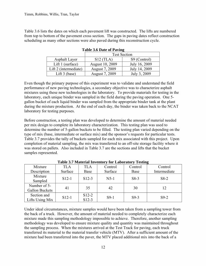
flatbed truck. The mixtures were then taken back to the parking lot behind the Test Track’s on-site laboratory for loading into buckets and storing on pallets (Figure 3.9).
a) Unloading Mix from Truck b) Sampling Mix
c) Loading Mix into Buckets d) Mix Storage
Figure 3.9 Mixture Sampling for Lab Testing Table 3.8 contains pertinent as-built information for each lift in each section. The binder used in the TLA mixes barely missed the requirements for a PG 76-22, which was the performance grade used in the TLA mix designs. The binder contents of the TLA intermediate and base mixes were slightly higher than those of the control mixes. The most noticeable differences between the corresponding mixes in the two test sections were the in-place air voids of the TLA mixes being 1.4, 2.4 and 1.3% lower than the control mixes, respectively.
Timm, Robbins, Willis, Tran, Taylor
14
Table 3.8 Asphalt Concrete Layer Properties – As Built Lift 1-Surface 2-Intermediate 3-Base
Section S12-TLA S9-Control S12-TLA S9-Control S12-TLA S9-ControlThickness, in. 1.4 1.2 2.9 2.8 2.6 3.0 NMASa, mm 9.5 9.5 19.0 19.0 19.0 19.0
%SBS 0 2.8 0 2.8 0 0.0 %TLA 25 0 25 0 25 0
PG Gradeb 76-16 82-22 76-16 82-22 76-16 76-22 Asphalt, % 6.1 6.1 4.7 4.4 4.9 4.7
Air Voids, % 5.5 6.9 4.8 7.2 6.1 7.4 Plant Temp, oFc 335 335 335 335 335 325 Paver Temp, oFd 283 275 293 316 293 254 Comp. Temp, oFe 247 264 243 273 248 243
aNominal Maximum Aggregate Size bSuperpave Asphalt Performance Grade conducted on extracted binders
cAsphalt plant mixing temperature dSurface temperature directly behind paver
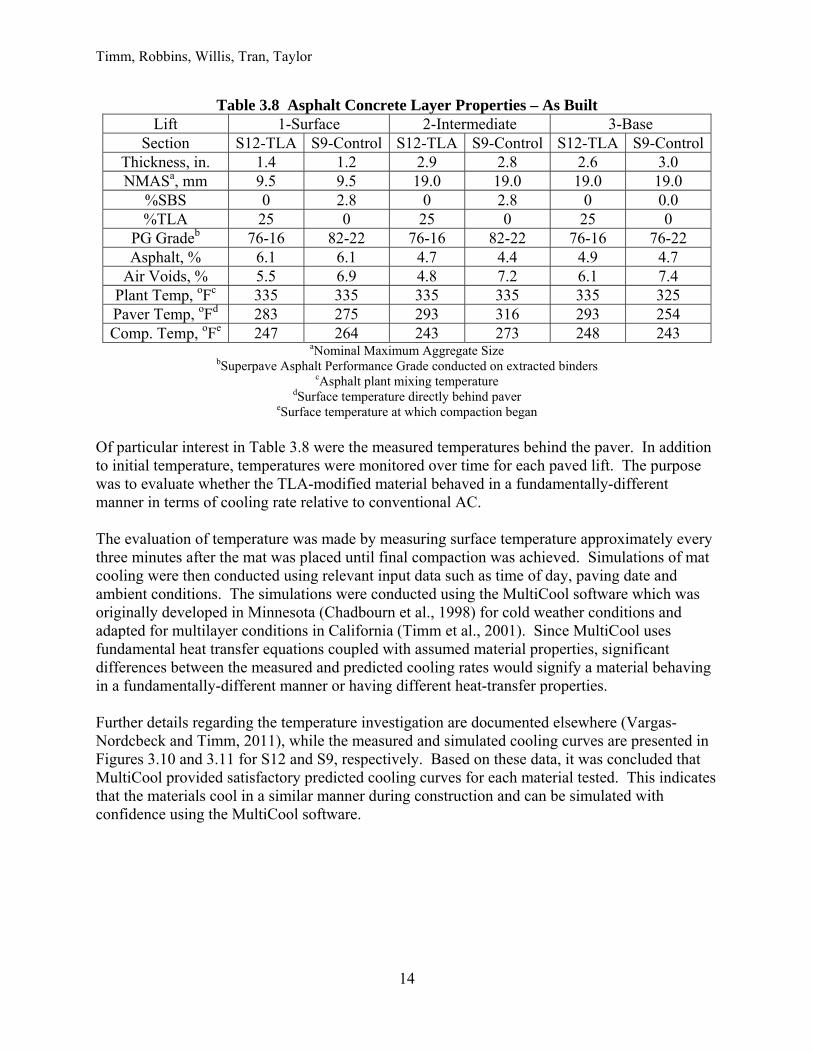
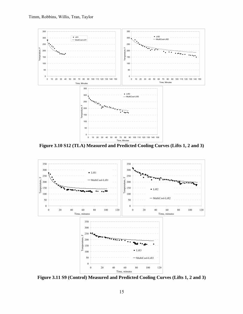
eSurface temperature at which compaction began Of particular interest in Table 3.8 were the measured temperatures behind the paver. In addition to initial temperature, temperatures were monitored over time for each paved lift. The purpose was to evaluate whether the TLA-modified material behaved in a fundamentally-different manner in terms of cooling rate relative to conventional AC. The evaluation of temperature was made by measuring surface temperature approximately every three minutes after the mat was placed until final compaction was achieved. Simulations of mat cooling were then conducted using relevant input data such as time of day, paving date and ambient conditions. The simulations were conducted using the MultiCool software which was originally developed in Minnesota (Chadbourn et al., 1998) for cold weather conditions and adapted for multilayer conditions in California (Timm et al., 2001). Since MultiCool uses fundamental heat transfer equations coupled with assumed material properties, significant differences between the measured and predicted cooling rates would signify a material behaving in a fundamentally-different manner or having different heat-transfer properties. Further details regarding the temperature investigation are documented elsewhere (Vargas-Nordcbeck and Timm, 2011), while the measured and simulated cooling curves are presented in Figures 3.10 and 3.11 for S12 and S9, respectively. Based on these data, it was concluded that MultiCool provided satisfactory predicted cooling curves for each material tested. This indicates that the materials cool in a similar manner during construction and can be simulated with confidence using the MultiCool software.
Timm, Robbins, Willis, Tran, Taylor
15
Figure 3.10 S12 (TLA) Measured and Predicted Cooling Curves (Lifts 1, 2 and 3)
Figure 3.11 S9 (Control) Measured and Predicted Cooling Curves (Lifts 1, 2 and 3)
0
50
100
150
200
250
300
350
0 10 20 30 40 50 60 70 80 90 100 110 120 130 140 150
Time, Minutes
Te
mp
erat
ure
, F
Lift1
MultiCool-Lift1
0
50
100
150
200
250
300
350
0 10 20 30 40 50 60 70 80 90 100 110 120 130 140 150
Time, Minutes
Tem
pera
ture
, F
Lift2MultiCool-Lift2
0
50
100
150
200
250
300
350
0 10 20 30 40 50 60 70 80 90 100 110 120 130 140 150
Time, Minutes
Te
mp
erat
ure
, F
Lift3MultiCool-Lift3
0
50
100
150
200
250
300
350
0 20 40 60 80 100 120
Time, minutes
Tem
pera
ture
, F
Lift1
MultiCool-Lift1
0
50
100
150
200
250
300
350
0 20 40 60 80 100 120
Time, minutes
Tem
pera
ture
, F
Lift2
MultiCool-Lift2
0
50
100
150
200
250
300
350
0 20 40 60 80 100 120
Time, minutes
Tem
pera
ture
, F
Lift3
MultiCool-Lift3
Timm, Robbins, Willis, Tran, Taylor
16
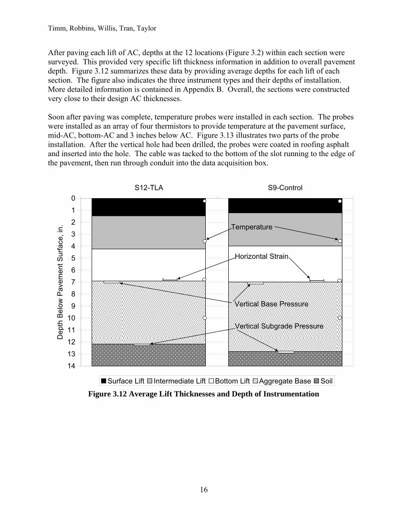
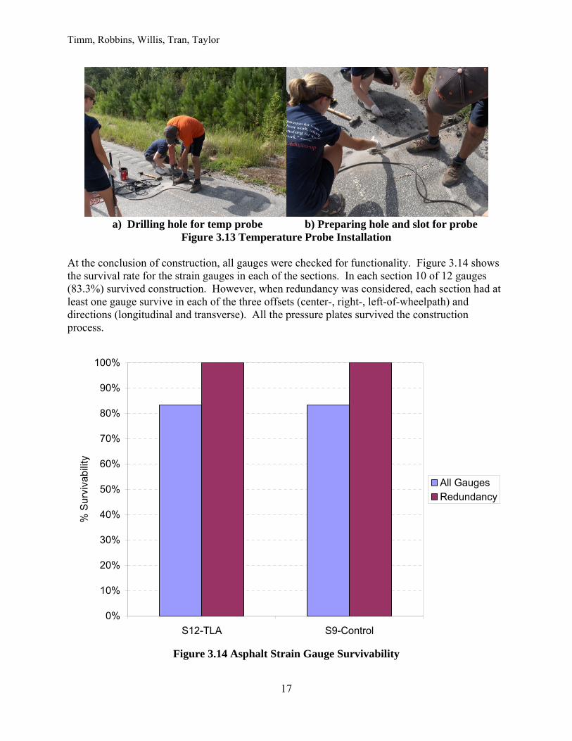
After paving each lift of AC, depths at the 12 locations (Figure 3.2) within each section were surveyed. This provided very specific lift thickness information in addition to overall pavement depth. Figure 3.12 summarizes these data by providing average depths for each lift of each section. The figure also indicates the three instrument types and their depths of installation. More detailed information is contained in Appendix B. Overall, the sections were constructed very close to their design AC thicknesses. Soon after paving was complete, temperature probes were installed in each section. The probes were installed as an array of four thermistors to provide temperature at the pavement surface, mid-AC, bottom-AC and 3 inches below AC. Figure 3.13 illustrates two parts of the probe installation. After the vertical hole had been drilled, the probes were coated in roofing asphalt and inserted into the hole. The cable was tacked to the bottom of the slot running to the edge of the pavement, then run through conduit into the data acquisition box.
Figure 3.12 Average Lift Thicknesses and Depth of Instrumentation
0
1
2
3
4
5
6
7
8
9
10
11
12
13
14
S12-TLA S9-Control
Dep
th B
elow
Pav
emen
t Sur
face
, in.
Surface Lift Intermediate Lift Bottom Lift Aggregate Base Soil
Temperature
Horizontal Strain
Vertical Base Pressure
Vertical Subgrade Pressure
Timm, Robbins, Willis, Tran, Taylor
17
a) Drilling hole for temp probe b) Preparing hole and slot for probe
Figure 3.13 Temperature Probe Installation At the conclusion of construction, all gauges were checked for functionality. Figure 3.14 shows the survival rate for the strain gauges in each of the sections. In each section 10 of 12 gauges (83.3%) survived construction. However, when redundancy was considered, each section had at least one gauge survive in each of the three offsets (center-, right-, left-of-wheelpath) and directions (longitudinal and transverse). All the pressure plates survived the construction process.
Figure 3.14 Asphalt Strain Gauge Survivability
0%
10%
20%
30%
40%
50%
60%
70%
80%
90%
100%
S12-TLA S9-Control
% S
urvi
vabi
lity
All GaugesRedundancy
Timm, Robbins, Willis, Tran, Taylor
18
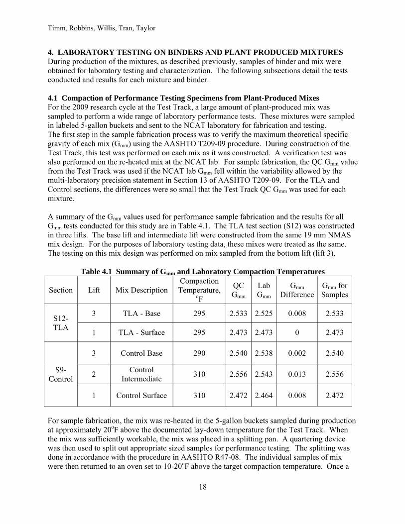
4. LABORATORY TESTING ON BINDERS AND PLANT PRODUCED MIXTURES During production of the mixtures, as described previously, samples of binder and mix were obtained for laboratory testing and characterization. The following subsections detail the tests conducted and results for each mixture and binder. 4.1 Compaction of Performance Testing Specimens from Plant-Produced Mixes For the 2009 research cycle at the Test Track, a large amount of plant-produced mix was sampled to perform a wide range of laboratory performance tests. These mixtures were sampled in labeled 5-gallon buckets and sent to the NCAT laboratory for fabrication and testing. The first step in the sample fabrication process was to verify the maximum theoretical specific gravity of each mix (Gmm) using the AASHTO T209-09 procedure. During construction of the Test Track, this test was performed on each mix as it was constructed. A verification test was also performed on the re-heated mix at the NCAT lab. For sample fabrication, the QC Gmm value from the Test Track was used if the NCAT lab Gmm fell within the variability allowed by the multi-laboratory precision statement in Section 13 of AASHTO T209-09. For the TLA and Control sections, the differences were so small that the Test Track QC Gmm was used for each mixture. A summary of the Gmm values used for performance sample fabrication and the results for all Gmm tests conducted for this study are in Table 4.1. The TLA test section (S12) was constructed in three lifts. The base lift and intermediate lift were constructed from the same 19 mm NMAS mix design. For the purposes of laboratory testing data, these mixes were treated as the same. The testing on this mix design was performed on mix sampled from the bottom lift (lift 3).
Table 4.1 Summary of Gmm and Laboratory Compaction Temperatures
Section Lift Mix Description Compaction Temperature,
oF
QC Gmm
Lab Gmm
Gmm Difference
Gmm for Samples
S12-TLA
3 TLA - Base 295 2.533 2.525 0.008 2.533
1 TLA - Surface 295 2.473 2.473 0 2.473
S9-Control
3 Control Base 290 2.540 2.538 0.002 2.540
2 Control
Intermediate 310 2.556 2.543 0.013 2.556
1 Control Surface 310 2.472 2.464 0.008 2.472
For sample fabrication, the mix was re-heated in the 5-gallon buckets sampled during production at approximately 20oF above the documented lay-down temperature for the Test Track. When the mix was sufficiently workable, the mix was placed in a splitting pan. A quartering device was then used to split out appropriate sized samples for performance testing. The splitting was done in accordance with the procedure in AASHTO R47-08. The individual samples of mix were then returned to an oven set to 10-20oF above the target compaction temperature. Once a
Timm, Robbins, Willis, Tran, Taylor
19
thermometer in the loose mix reached the target compaction temperature, the mix was compacted into the appropriately sized performance testing sample. No short-term mechanical aging (AASHTO R30) was conducted on the plant-produced mixes from the Test Track since these mixes had already been short-term aged during the production process. More discussion of sample properties will be provided (sample height, target air voids, etc.) when the individual performance tests are discussed. A summary of the target compaction temperatures for this project is provided in Table 4.1. 4.2 Binder Properties The binders used to produce the asphalt mixtures for Sections S9 and S12 were sampled at the plant (hereafter referred to as the tank binders) and extracted from the mixes sampled during construction (hereafter referred to as the extracted binders) for testing. The tank and extracted binders were tested and graded according to the Superpave performance grading procedure (AASHTO M 320-10). In addition, the Multiple Stress Creep Recovery (MSCR) test was also conducted to grade these binders in compliance with AASHTO MP 19-10. Testing results are described in the following subsections.
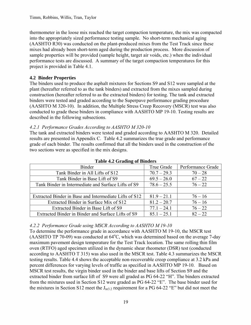
4.2.1 Performance Grades According to AASHTO M 320-10 The tank and extracted binders were tested and graded according to AASHTO M 320. Detailed results are presented in Appendix C. Table 4.2 summarizes the true grade and performance grade of each binder. The results confirmed that all the binders used in the construction of the two sections were as specified in the mix designs.
Table 4.2 Grading of Binders Binder True Grade Performance Grade
Tank Binder in All Lifts of S12 70.7 – 29.3 70 – 28 Tank Binder in Base Lift of S9 69.5 – 26.0 67 – 22
Tank Binder in Intermediate and Surface Lifts of S9 78.6 – 25.5 76 – 22
Extracted Binder in Base and Intermediate Lifts of S12 81.9 – 21.1 76 – 16 Extracted Binder in Surface Mix of S12 81.2 – 20.7 76 – 16
Extracted Binder in Base Lift of S9 77.1 – 24.1 76 – 22 Extracted Binder in Binder and Surface Lifts of S9 85.1 – 25.1 82 – 22
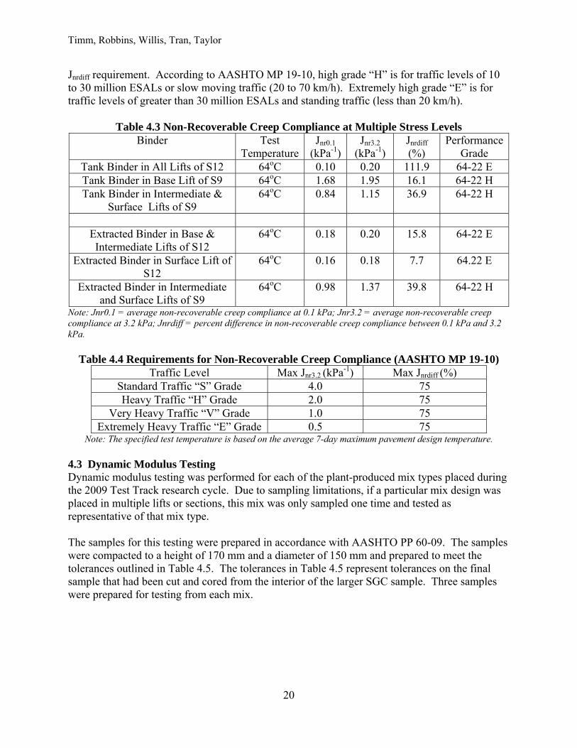
4.2.2 Performance Grade using MSCR According to AASHTO M 19-10 To determine the performance grade in accordance with AASHTO M 19-10, the MSCR test (AASHTO TP 70-09) was conducted at 64oC, which was determined based on the average 7-day maximum pavement design temperature for the Test Track location. The same rolling thin film oven (RTFO) aged specimen utilized in the dynamic shear rheometer (DSR) test (conducted according to AASHTO T 315) was also used in the MSCR test. Table 4.3 summarizes the MSCR testing results. Table 4.4 shows the acceptable non-recoverable creep compliance at 3.2 kPa and percent differences for varying levels of traffic as specified in AASHTO MP 19-10. Based on MSCR test results, the virgin binder used in the binder and base lifts of Section S9 and the extracted binder from surface lift of S9 were all graded as PG 64-22 “H”. The binders extracted from the mixtures used in Section S12 were graded as PG 64-22 “E”. The base binder used for the mixtures in Section S12 meet the Jnr3.2 requirement for a PG 64-22 “E” but did not meet the
Timm, Robbins, Willis, Tran, Taylor
20
Jnrdiff requirement. According to AASHTO MP 19-10, high grade “H” is for traffic levels of 10 to 30 million ESALs or slow moving traffic (20 to 70 km/h). Extremely high grade “E” is for traffic levels of greater than 30 million ESALs and standing traffic (less than 20 km/h).
Table 4.3 Non-Recoverable Creep Compliance at Multiple Stress Levels Binder Test
TemperatureJnr0.1
(kPa-1)Jnr3.2
(kPa-1) Jnrdiff
(%) Performance
Grade Tank Binder in All Lifts of S12 64oC 0.10 0.20 111.9 64-22 E Tank Binder in Base Lift of S9 64oC 1.68 1.95 16.1 64-22 H Tank Binder in Intermediate &
Surface Lifts of S9 64oC 0.84 1.15 36.9 64-22 H
Extracted Binder in Base & Intermediate Lifts of S12
64oC 0.18 0.20 15.8 64-22 E
Extracted Binder in Surface Lift of S12
64oC 0.16 0.18 7.7 64.22 E
Extracted Binder in Intermediate and Surface Lifts of S9
64oC 0.98 1.37 39.8 64-22 H
Note: Jnr0.1 = average non-recoverable creep compliance at 0.1 kPa; Jnr3.2 = average non-recoverable creep compliance at 3.2 kPa; Jnrdiff = percent difference in non-recoverable creep compliance between 0.1 kPa and 3.2 kPa.
Table 4.4 Requirements for Non-Recoverable Creep Compliance (AASHTO MP 19-10) Traffic Level Max Jnr3.2 (kPa-1) Max Jnrdiff (%)
Standard Traffic “S” Grade 4.0 75 Heavy Traffic “H” Grade 2.0 75
Very Heavy Traffic “V” Grade 1.0 75 Extremely Heavy Traffic “E” Grade 0.5 75
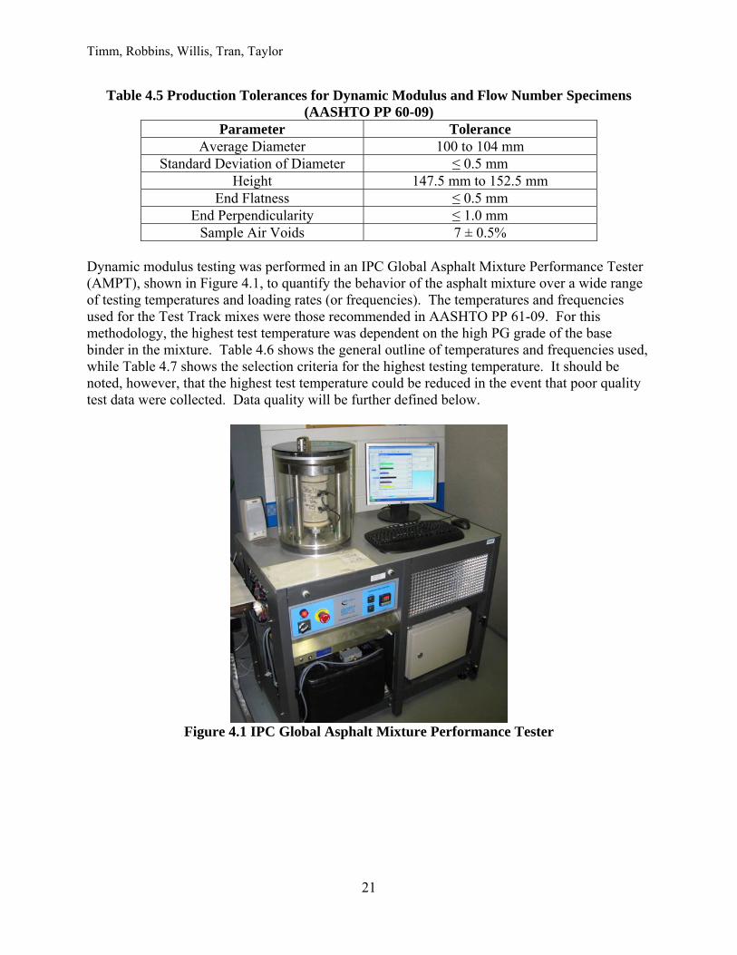
Note: The specified test temperature is based on the average 7-day maximum pavement design temperature. 4.3 Dynamic Modulus Testing Dynamic modulus testing was performed for each of the plant-produced mix types placed during the 2009 Test Track research cycle. Due to sampling limitations, if a particular mix design was placed in multiple lifts or sections, this mix was only sampled one time and tested as representative of that mix type. The samples for this testing were prepared in accordance with AASHTO PP 60-09. The samples were compacted to a height of 170 mm and a diameter of 150 mm and prepared to meet the tolerances outlined in Table 4.5. The tolerances in Table 4.5 represent tolerances on the final sample that had been cut and cored from the interior of the larger SGC sample. Three samples were prepared for testing from each mix.
Timm, Robbins, Willis, Tran, Taylor
21
Table 4.5 Production Tolerances for Dynamic Modulus and Flow Number Specimens (AASHTO PP 60-09)
Parameter Tolerance Average Diameter 100 to 104 mm
Standard Deviation of Diameter ≤ 0.5 mm Height 147.5 mm to 152.5 mm
End Flatness ≤ 0.5 mm End Perpendicularity ≤ 1.0 mm
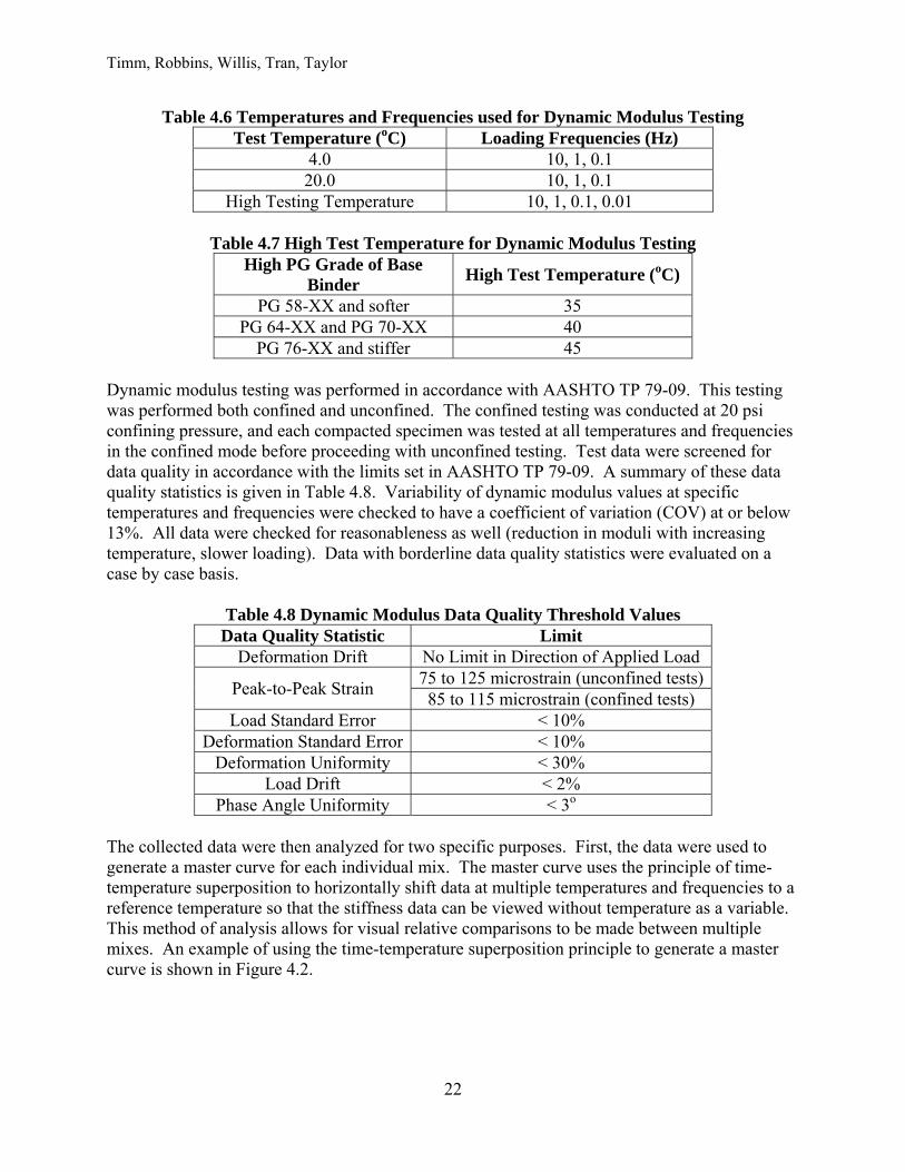
Sample Air Voids 7 ± 0.5% Dynamic modulus testing was performed in an IPC Global Asphalt Mixture Performance Tester (AMPT), shown in Figure 4.1, to quantify the behavior of the asphalt mixture over a wide range of testing temperatures and loading rates (or frequencies). The temperatures and frequencies used for the Test Track mixes were those recommended in AASHTO PP 61-09. For this methodology, the highest test temperature was dependent on the high PG grade of the base binder in the mixture. Table 4.6 shows the general outline of temperatures and frequencies used, while Table 4.7 shows the selection criteria for the highest testing temperature. It should be noted, however, that the highest test temperature could be reduced in the event that poor quality test data were collected. Data quality will be further defined below.
Figure 4.1 IPC Global Asphalt Mixture Performance Tester
Timm, Robbins, Willis, Tran, Taylor
22
Table 4.6 Temperatures and Frequencies used for Dynamic Modulus Testing Test Temperature (oC) Loading Frequencies (Hz)
4.0 10, 1, 0.1 20.0 10, 1, 0.1
High Testing Temperature 10, 1, 0.1, 0.01
Table 4.7 High Test Temperature for Dynamic Modulus Testing High PG Grade of Base
Binder High Test Temperature (oC)
PG 58-XX and softer 35 PG 64-XX and PG 70-XX 40
PG 76-XX and stiffer 45
Dynamic modulus testing was performed in accordance with AASHTO TP 79-09. This testing was performed both confined and unconfined. The confined testing was conducted at 20 psi confining pressure, and each compacted specimen was tested at all temperatures and frequencies in the confined mode before proceeding with unconfined testing. Test data were screened for data quality in accordance with the limits set in AASHTO TP 79-09. A summary of these data quality statistics is given in Table 4.8. Variability of dynamic modulus values at specific temperatures and frequencies were checked to have a coefficient of variation (COV) at or below 13%. All data were checked for reasonableness as well (reduction in moduli with increasing temperature, slower loading). Data with borderline data quality statistics were evaluated on a case by case basis.
Table 4.8 Dynamic Modulus Data Quality Threshold Values
Data Quality Statistic Limit Deformation Drift No Limit in Direction of Applied Load
Peak-to-Peak Strain 75 to 125 microstrain (unconfined tests) 85 to 115 microstrain (confined tests)
Load Standard Error < 10% Deformation Standard Error < 10%
Deformation Uniformity < 30% Load Drift < 2%
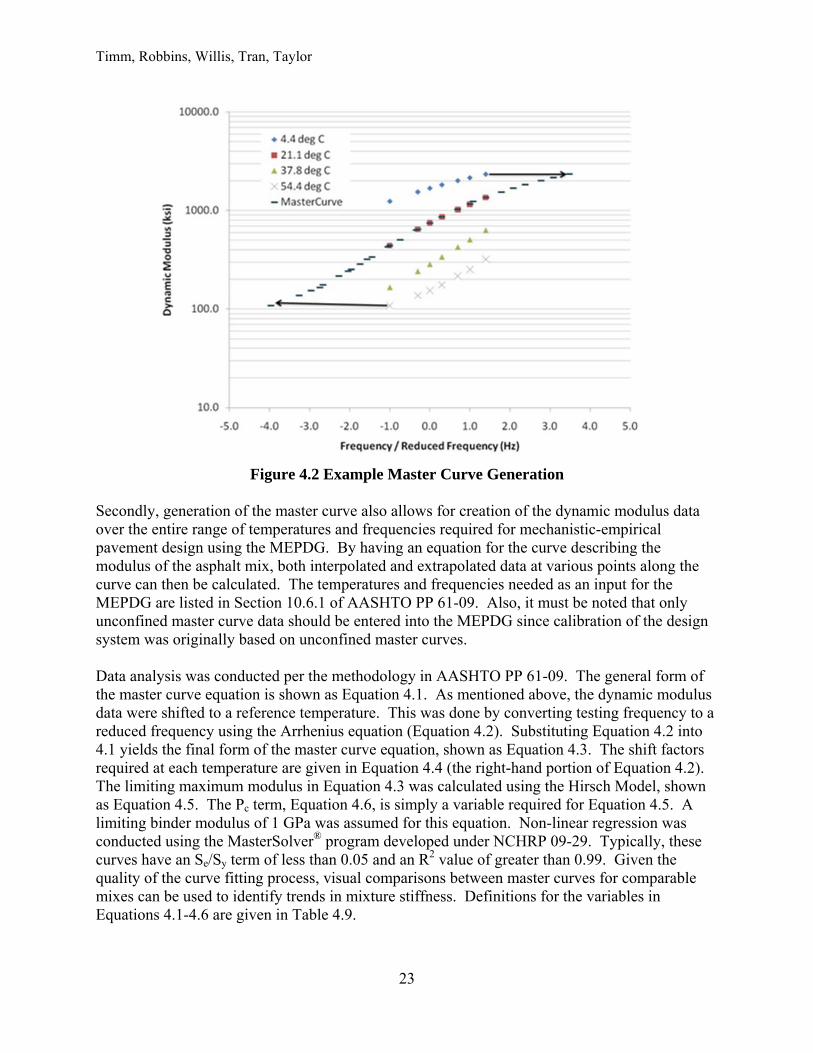
Phase Angle Uniformity < 3o The collected data were then analyzed for two specific purposes. First, the data were used to generate a master curve for each individual mix. The master curve uses the principle of time-temperature superposition to horizontally shift data at multiple temperatures and frequencies to a reference temperature so that the stiffness data can be viewed without temperature as a variable. This method of analysis allows for visual relative comparisons to be made between multiple mixes. An example of using the time-temperature superposition principle to generate a master curve is shown in Figure 4.2.
Timm, Robbins, Willis, Tran, Taylor
23
Figure 4.2 Example Master Curve Generation
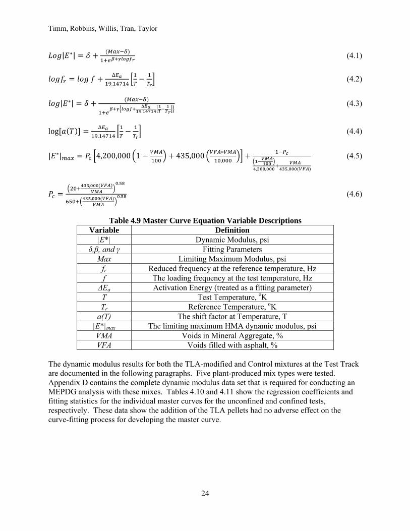
Secondly, generation of the master curve also allows for creation of the dynamic modulus data over the entire range of temperatures and frequencies required for mechanistic-empirical pavement design using the MEPDG. By having an equation for the curve describing the modulus of the asphalt mix, both interpolated and extrapolated data at various points along the curve can then be calculated. The temperatures and frequencies needed as an input for the MEPDG are listed in Section 10.6.1 of AASHTO PP 61-09. Also, it must be noted that only unconfined master curve data should be entered into the MEPDG since calibration of the design system was originally based on unconfined master curves. Data analysis was conducted per the methodology in AASHTO PP 61-09. The general form of the master curve equation is shown as Equation 4.1. As mentioned above, the dynamic modulus data were shifted to a reference temperature. This was done by converting testing frequency to a reduced frequency using the Arrhenius equation (Equation 4.2). Substituting Equation 4.2 into 4.1 yields the final form of the master curve equation, shown as Equation 4.3. The shift factors required at each temperature are given in Equation 4.4 (the right-hand portion of Equation 4.2). The limiting maximum modulus in Equation 4.3 was calculated using the Hirsch Model, shown as Equation 4.5. The Pc term, Equation 4.6, is simply a variable required for Equation 4.5. A limiting binder modulus of 1 GPa was assumed for this equation. Non-linear regression was conducted using the MasterSolver® program developed under NCHRP 09-29. Typically, these curves have an Se/Sy term of less than 0.05 and an R2 value of greater than 0.99. Given the quality of the curve fitting process, visual comparisons between master curves for comparable mixes can be used to identify trends in mixture stiffness. Definitions for the variables in Equations 4.1-4.6 are given in Table 4.9.
Timm, Robbins, Willis, Tran, Taylor
24
| ∗| (4.1)
∆
. (4.2)
| ∗| ∆.
(4.3)
log ∆
. (4.4)
| ∗| 4,200,000 1 435,000 ∗
,, , ,
(4.5)
, .
, . (4.6)
Table 4.9 Master Curve Equation Variable Descriptions
Variable Definition |E*| Dynamic Modulus, psi
δ,β, and γ Fitting Parameters Max Limiting Maximum Modulus, psi
fr Reduced frequency at the reference temperature, Hz f The loading frequency at the test temperature, Hz ΔEa Activation Energy (treated as a fitting parameter) T Test Temperature, oK Tr Reference Temperature, oK
a(T) The shift factor at Temperature, T |E*|max The limiting maximum HMA dynamic modulus, psi VMA Voids in Mineral Aggregate, % VFA Voids filled with asphalt, %
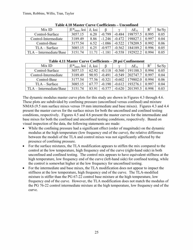
The dynamic modulus results for both the TLA-modified and Control mixtures at the Test Track are documented in the following paragraphs. Five plant-produced mix types were tested. Appendix D contains the complete dynamic modulus data set that is required for conducting an MEPDG analysis with these mixes. Tables 4.10 and 4.11 show the regression coefficients and fitting statistics for the individual master curves for the unconfined and confined tests, respectively. These data show the addition of the TLA pellets had no adverse effect on the curve-fitting process for developing the master curve.
Timm, Robbins, Willis, Tran, Taylor
25
Table 4.10 Master Curve Coefficients – Unconfined Mix ID |E*|max, ksi , ksi EA R2 Se/Sy
Control-Surface 3057.15 6.20 -0.799 -0.484 198757.5 0.995 0.05 Control-Intermediate 3189.49 8.86 -1.246 -0.472 198827.1 0.997 0.04
Control-Base 3177.54 6.52 -1.086 -0.522 178209.5 0.992 0.06 TLA – Surface 3085.15 6.25 -0.977 -0.562 184189.2 0.996 0.05
TLA – Intermediate/Base 3151.74 11.71 -1.181 -0.558 192922.2 0.994 0.05
Table 4.11 Master Curve Coefficients – 20 psi Confinement Mix ID |E*|max, ksi , ksi EA R2 Se/Sy
Control-Surface 3057.15 62.92 -0.118 -0.560 191188.3 0.994 0.05 Control-Intermediate 3189.49 90.93 -0.491 -0.549 202747.7 0.997 0.04
Control-Base 3177.54 77.56 -0.321 -0.602 179802.0 0.994 0.06 TLA – Surface 3085.15 67.77 -0.190 -0.612 193276.1 0.997 0.04
TLA – Intermediate/Base 3151.74 83.91 -0.577 -0.620 201395.5 0.998 0.03
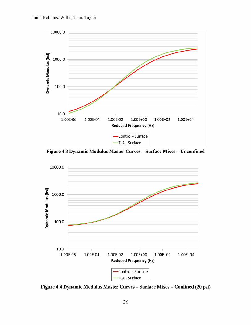
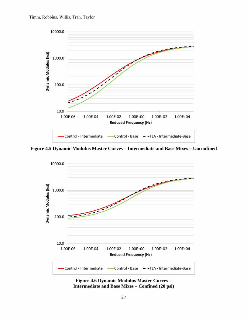
The dynamic modulus master curve plots for this study are shown in Figures 4.3 through 4.6. These plots are subdivided by confining pressure (unconfined versus confined) and mixture NMAS (9.5 mm surface mixes versus 19 mm intermediate and base mixes). Figures 4.3 and 4.4 present the master curves for the surface mixes for both the unconfined and confined testing conditions, respectively. Figures 4.5 and 4.6 present the master curves for the intermediate and base mixes for both the confined and unconfined testing conditions, respectively. Based on visual inspection of the data, the following statements are made: While the confining pressure had a significant effect (order of magnitude) on the dynamic
modulus at the high temperature (low frequency end of the curve), the relative difference between the moduli of the TLA and control mixes was not significantly affected by the presence of confining pressure.
For the surface mixtures, the TLA modification appears to stiffen the mix compared to the control at the low temperature, high frequency end of the curve (right-hand side) in both unconfined and confined testing. The control mix appears to have equivalent stiffness at the high temperature, low frequency end of the curve (left-hand side) for confined testing, while the control is somewhat higher at the low frequency for unconfined testing.
For the intermediate and base mixes, the TLA modification does not appear to impact the stiffness at the low temperature, high frequency end of the curve. The TLA-modified mixture is stiffer than the PG 67-22 control base mixture at the high temperature, low frequency end of the curve. However, the TLA modification does not match the modulus of the PG 76-22 control intermediate mixture at the high temperature, low frequency end of the curve.
Timm, Robbins, Willis, Tran, Taylor
26
Figure 4.3 Dynamic Modulus Master Curves – Surface Mixes – Unconfined
Figure 4.4 Dynamic Modulus Master Curves – Surface Mixes – Confined (20 psi)
Timm, Robbins, Willis, Tran, Taylor
27
Figure 4.5 Dynamic Modulus Master Curves – Intermediate and Base Mixes – Unconfined
Figure 4.6 Dynamic Modulus Master Curves –
Intermediate and Base Mixes – Confined (20 psi)
Timm, Robbins, Willis, Tran, Taylor
28
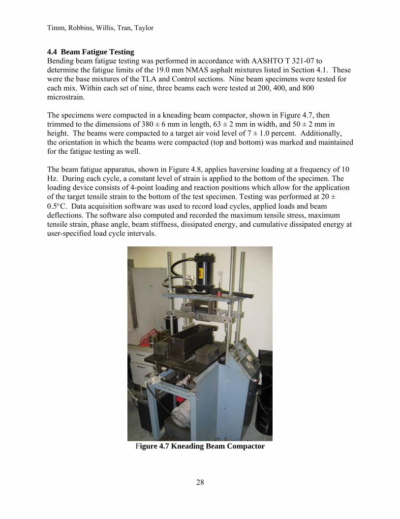
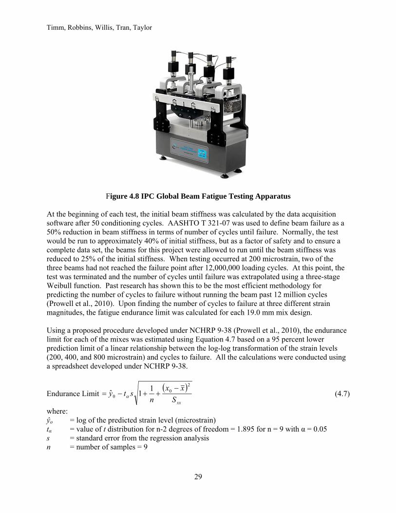
4.4 Beam Fatigue Testing Bending beam fatigue testing was performed in accordance with AASHTO T 321-07 to determine the fatigue limits of the 19.0 mm NMAS asphalt mixtures listed in Section 4.1. These were the base mixtures of the TLA and Control sections. Nine beam specimens were tested for each mix. Within each set of nine, three beams each were tested at 200, 400, and 800 microstrain. The specimens were compacted in a kneading beam compactor, shown in Figure 4.7, then trimmed to the dimensions of 380 ± 6 mm in length, 63 ± 2 mm in width, and 50 ± 2 mm in height. The beams were compacted to a target air void level of 7 ± 1.0 percent. Additionally, the orientation in which the beams were compacted (top and bottom) was marked and maintained for the fatigue testing as well. The beam fatigue apparatus, shown in Figure 4.8, applies haversine loading at a frequency of 10 Hz. During each cycle, a constant level of strain is applied to the bottom of the specimen. The loading device consists of 4-point loading and reaction positions which allow for the application of the target tensile strain to the bottom of the test specimen. Testing was performed at 20 ± 0.5C. Data acquisition software was used to record load cycles, applied loads and beam deflections. The software also computed and recorded the maximum tensile stress, maximum tensile strain, phase angle, beam stiffness, dissipated energy, and cumulative dissipated energy at user-specified load cycle intervals.
Figure 4.7 Kneading Beam Compactor
Timm, Robbins, Willis, Tran, Taylor
29
Figure 4.8 IPC Global Beam Fatigue Testing Apparatus At the beginning of each test, the initial beam stiffness was calculated by the data acquisition software after 50 conditioning cycles. AASHTO T 321-07 was used to define beam failure as a 50% reduction in beam stiffness in terms of number of cycles until failure. Normally, the test would be run to approximately 40% of initial stiffness, but as a factor of safety and to ensure a complete data set, the beams for this project were allowed to run until the beam stiffness was reduced to 25% of the initial stiffness. When testing occurred at 200 microstrain, two of the three beams had not reached the failure point after 12,000,000 loading cycles. At this point, the test was terminated and the number of cycles until failure was extrapolated using a three-stage Weibull function. Past research has shown this to be the most efficient methodology for predicting the number of cycles to failure without running the beam past 12 million cycles (Prowell et al., 2010). Upon finding the number of cycles to failure at three different strain magnitudes, the fatigue endurance limit was calculated for each 19.0 mm mix design. Using a proposed procedure developed under NCHRP 9-38 (Prowell et al., 2010), the endurance limit for each of the mixes was estimated using Equation 4.7 based on a 95 percent lower prediction limit of a linear relationship between the log-log transformation of the strain levels (200, 400, and 800 microstrain) and cycles to failure. All the calculations were conducted using a spreadsheet developed under NCHRP 9-38.
Endurance Limit
xxS
xx
nsty
20
0
11ˆ
(4.7)
where: ŷo = log of the predicted strain level (microstrain) tα = value of t distribution for n-2 degrees of freedom = 1.895 for n = 9 with α = 0.05 s = standard error from the regression analysis n = number of samples = 9
Timm, Robbins, Willis, Tran, Taylor
30
Sxx =
n
ii xx
1
2 (Note: log of fatigue lives)
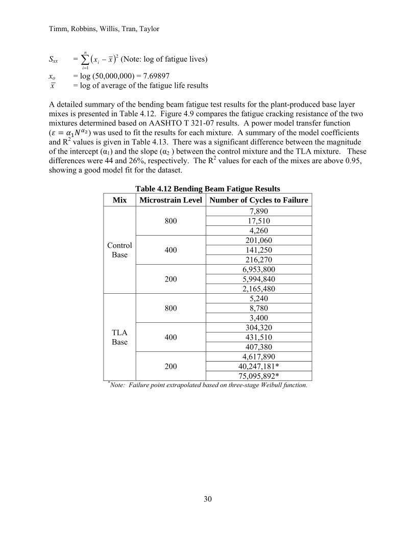
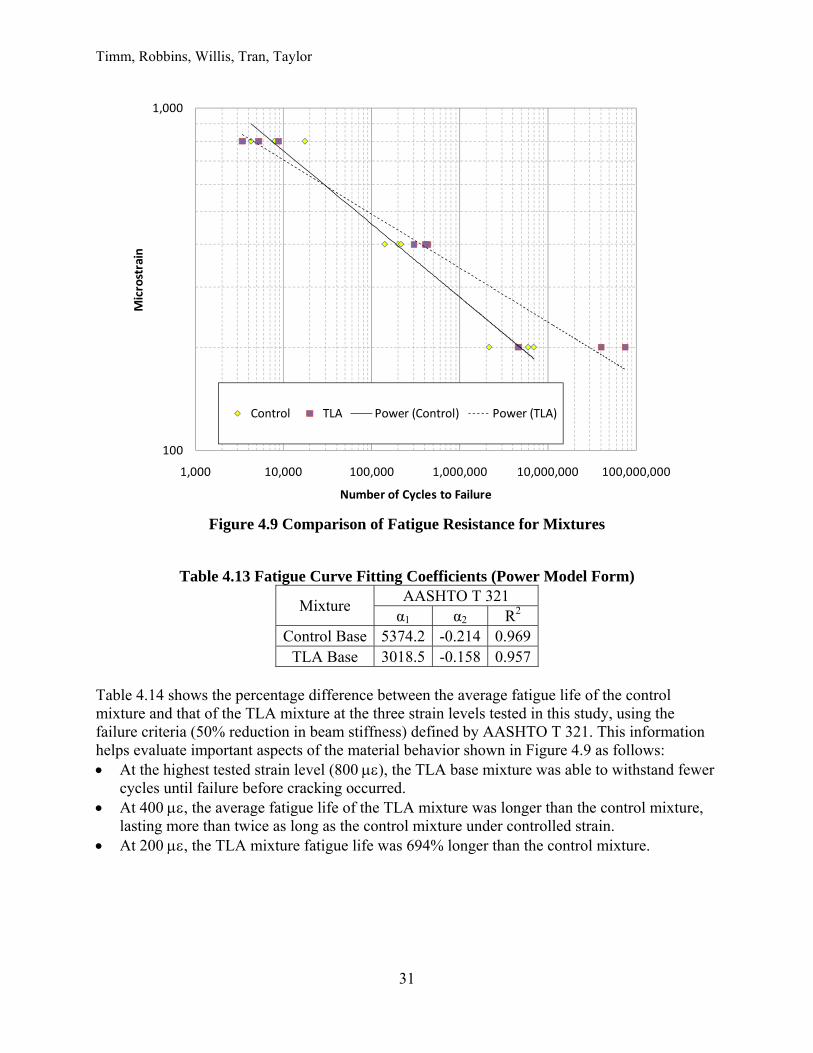
xo = log (50,000,000) = 7.69897 x = log of average of the fatigue life results A detailed summary of the bending beam fatigue test results for the plant-produced base layer mixes is presented in Table 4.12. Figure 4.9 compares the fatigue cracking resistance of the two mixtures determined based on AASHTO T 321-07 results. A power model transfer function ( ) was used to fit the results for each mixture. A summary of the model coefficients and R2 values is given in Table 4.13. There was a significant difference between the magnitude of the intercept (α1) and the slope (α2 ) between the control mixture and the TLA mixture. These differences were 44 and 26%, respectively. The R2 values for each of the mixes are above 0.95, showing a good model fit for the dataset.
Table 4.12 Bending Beam Fatigue Results
Mix Microstrain Level Number of Cycles to Failure
Control Base
800 7,890 17,510 4,260
400 201,060 141,250 216,270
200 6,953,800 5,994,840 2,165,480
TLA Base
800 5,240 8,780 3,400
400 304,320 431,510 407,380
200 4,617,890
40,247,181* 75,095,892*
*Note: Failure point extrapolated based on three-stage Weibull function.
Timm, Robbins, Willis, Tran, Taylor
31
Figure 4.9 Comparison of Fatigue Resistance for Mixtures
Table 4.13 Fatigue Curve Fitting Coefficients (Power Model Form)
Mixture AASHTO T 321 α1 α2 R2
Control Base 5374.2 -0.214 0.969TLA Base 3018.5 -0.158 0.957
Table 4.14 shows the percentage difference between the average fatigue life of the control mixture and that of the TLA mixture at the three strain levels tested in this study, using the failure criteria (50% reduction in beam stiffness) defined by AASHTO T 321. This information helps evaluate important aspects of the material behavior shown in Figure 4.9 as follows: At the highest tested strain level (800 ), the TLA base mixture was able to withstand fewer
cycles until failure before cracking occurred. At 400 , the average fatigue life of the TLA mixture was longer than the control mixture,
lasting more than twice as long as the control mixture under controlled strain. At 200 , the TLA mixture fatigue life was 694% longer than the control mixture.
100
1,000
1,000 10,000 100,000 1,000,000 10,000,000 100,000,000
Microstrain
Number of Cycles to Failure
Control TLA Power (Control) Power (TLA)
Timm, Robbins, Willis, Tran, Taylor
32
Table 4.14 Percent Increase in Cycles to Failure for TLA versus Control Mixture Strain Level 200 400 800
Percent Increase in Predicted Life 694% 105% -41.3% Table 4.15 shows the 95 percent one-sided lower prediction of endurance limit for each of the two mixes tested in this study based on the number of cycles to failure determined in accordance with AASHTO T 321. The procedure for estimating the endurance limit was developed under NCHRP 9-38 (Prowell et al., 2010). Based on the results shown in Table 4.15, the TLA base mixture had a fatigue endurance limit 20% higher than the control mixture.
Table 4.15 Predicted Endurance Limits Mixture Endurance Limit (Microstrain)
Control Base 99 TLA Base 119
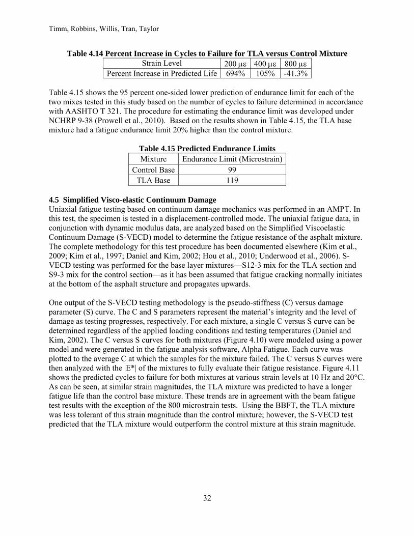
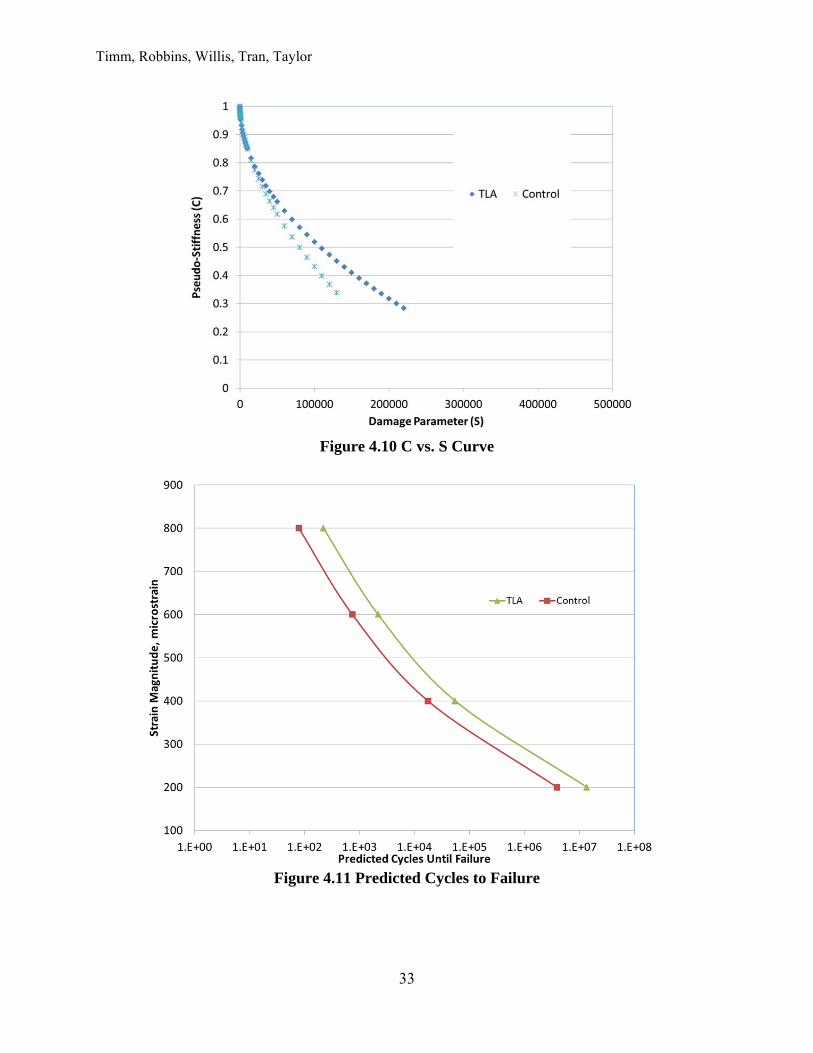
4.5 Simplified Visco-elastic Continuum Damage Uniaxial fatigue testing based on continuum damage mechanics was performed in an AMPT. In this test, the specimen is tested in a displacement-controlled mode. The uniaxial fatigue data, in conjunction with dynamic modulus data, are analyzed based on the Simplified Viscoelastic Continuum Damage (S-VECD) model to determine the fatigue resistance of the asphalt mixture. The complete methodology for this test procedure has been documented elsewhere (Kim et al., 2009; Kim et al., 1997; Daniel and Kim, 2002; Hou et al., 2010; Underwood et al., 2006). S-VECD testing was performed for the base layer mixtures—S12-3 mix for the TLA section and S9-3 mix for the control section—as it has been assumed that fatigue cracking normally initiates at the bottom of the asphalt structure and propagates upwards. One output of the S-VECD testing methodology is the pseudo-stiffness (C) versus damage parameter (S) curve. The C and S parameters represent the material’s integrity and the level of damage as testing progresses, respectively. For each mixture, a single C versus S curve can be determined regardless of the applied loading conditions and testing temperatures (Daniel and Kim, 2002). The C versus S curves for both mixtures (Figure 4.10) were modeled using a power model and were generated in the fatigue analysis software, Alpha Fatigue. Each curve was plotted to the average C at which the samples for the mixture failed. The C versus S curves were then analyzed with the |E*| of the mixtures to fully evaluate their fatigue resistance. Figure 4.11 shows the predicted cycles to failure for both mixtures at various strain levels at 10 Hz and 20°C. As can be seen, at similar strain magnitudes, the TLA mixture was predicted to have a longer fatigue life than the control base mixture. These trends are in agreement with the beam fatigue test results with the exception of the 800 microstrain tests. Using the BBFT, the TLA mixture was less tolerant of this strain magnitude than the control mixture; however, the S-VECD test predicted that the TLA mixture would outperform the control mixture at this strain magnitude.
Timm, Robbins, Willis, Tran, Taylor
33
Figure 4.10 C vs. S Curve
Figure 4.11 Predicted Cycles to Failure
Timm, Robbins, Willis, Tran, Taylor
34
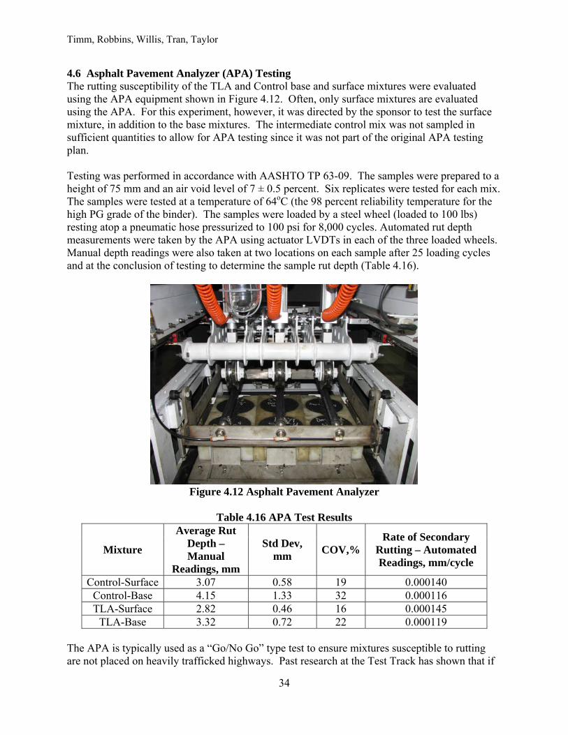
4.6 Asphalt Pavement Analyzer (APA) Testing The rutting susceptibility of the TLA and Control base and surface mixtures were evaluated using the APA equipment shown in Figure 4.12. Often, only surface mixtures are evaluated using the APA. For this experiment, however, it was directed by the sponsor to test the surface mixture, in addition to the base mixtures. The intermediate control mix was not sampled in sufficient quantities to allow for APA testing since it was not part of the original APA testing plan. Testing was performed in accordance with AASHTO TP 63-09. The samples were prepared to a height of 75 mm and an air void level of 7 ± 0.5 percent. Six replicates were tested for each mix. The samples were tested at a temperature of 64oC (the 98 percent reliability temperature for the high PG grade of the binder). The samples were loaded by a steel wheel (loaded to 100 lbs) resting atop a pneumatic hose pressurized to 100 psi for 8,000 cycles. Automated rut depth measurements were taken by the APA using actuator LVDTs in each of the three loaded wheels. Manual depth readings were also taken at two locations on each sample after 25 loading cycles and at the conclusion of testing to determine the sample rut depth (Table 4.16).
Figure 4.12 Asphalt Pavement Analyzer
Table 4.16 APA Test Results
Mixture
Average Rut Depth – Manual
Readings, mm
Std Dev, mm
COV,%Rate of Secondary
Rutting – Automated Readings, mm/cycle
Control-Surface 3.07 0.58 19 0.000140 Control-Base 4.15 1.33 32 0.000116 TLA-Surface 2.82 0.46 16 0.000145
TLA-Base 3.32 0.72 22 0.000119 The APA is typically used as a “Go/No Go” type test to ensure mixtures susceptible to rutting are not placed on heavily trafficked highways. Past research at the Test Track has shown that if
Timm, Robbins, Willis, Tran, Taylor
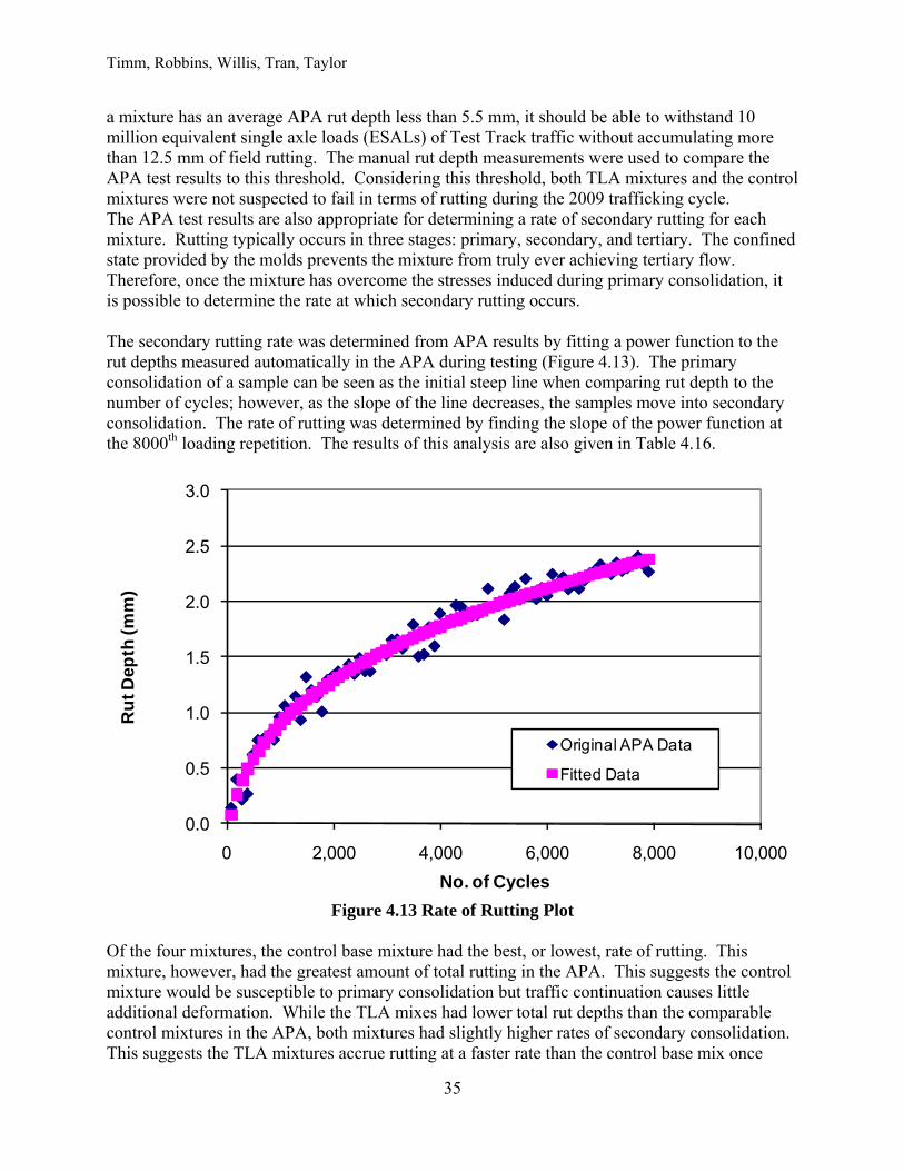
35
a mixture has an average APA rut depth less than 5.5 mm, it should be able to withstand 10 million equivalent single axle loads (ESALs) of Test Track traffic without accumulating more than 12.5 mm of field rutting. The manual rut depth measurements were used to compare the APA test results to this threshold. Considering this threshold, both TLA mixtures and the control mixtures were not suspected to fail in terms of rutting during the 2009 trafficking cycle. The APA test results are also appropriate for determining a rate of secondary rutting for each mixture. Rutting typically occurs in three stages: primary, secondary, and tertiary. The confined state provided by the molds prevents the mixture from truly ever achieving tertiary flow. Therefore, once the mixture has overcome the stresses induced during primary consolidation, it is possible to determine the rate at which secondary rutting occurs. The secondary rutting rate was determined from APA results by fitting a power function to the rut depths measured automatically in the APA during testing (Figure 4.13). The primary consolidation of a sample can be seen as the initial steep line when comparing rut depth to the number of cycles; however, as the slope of the line decreases, the samples move into secondary consolidation. The rate of rutting was determined by finding the slope of the power function at the 8000th loading repetition. The results of this analysis are also given in Table 4.16.
Figure 4.13 Rate of Rutting Plot
Of the four mixtures, the control base mixture had the best, or lowest, rate of rutting. This mixture, however, had the greatest amount of total rutting in the APA. This suggests the control mixture would be susceptible to primary consolidation but traffic continuation causes little additional deformation. While the TLA mixes had lower total rut depths than the comparable control mixtures in the APA, both mixtures had slightly higher rates of secondary consolidation. This suggests the TLA mixtures accrue rutting at a faster rate than the control base mix once
0.0
0.5
1.0
1.5
2.0
2.5
3.0
0 2,000 4,000 6,000 8,000 10,000
Ru
t Dep
th (m
m)
No. of Cycles
Original APA Data
Fitted Data
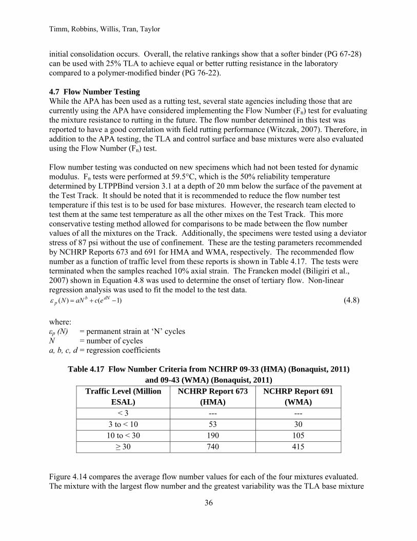
Timm, Robbins, Willis, Tran, Taylor
36
initial consolidation occurs. Overall, the relative rankings show that a softer binder (PG 67-28) can be used with 25% TLA to achieve equal or better rutting resistance in the laboratory compared to a polymer-modified binder (PG 76-22). 4.7 Flow Number Testing While the APA has been used as a rutting test, several state agencies including those that are currently using the APA have considered implementing the Flow Number (Fn) test for evaluating the mixture resistance to rutting in the future. The flow number determined in this test was reported to have a good correlation with field rutting performance (Witczak, 2007). Therefore, in addition to the APA testing, the TLA and control surface and base mixtures were also evaluated using the Flow Number (Fn) test. Flow number testing was conducted on new specimens which had not been tested for dynamic modulus. Fn tests were performed at 59.5°C, which is the 50% reliability temperature determined by LTPPBind version 3.1 at a depth of 20 mm below the surface of the pavement at the Test Track. It should be noted that it is recommended to reduce the flow number test temperature if this test is to be used for base mixtures. However, the research team elected to test them at the same test temperature as all the other mixes on the Test Track. This more conservative testing method allowed for comparisons to be made between the flow number values of all the mixtures on the Track. Additionally, the specimens were tested using a deviator stress of 87 psi without the use of confinement. These are the testing parameters recommended by NCHRP Reports 673 and 691 for HMA and WMA, respectively. The recommended flow number as a function of traffic level from these reports is shown in Table 4.17. The tests were terminated when the samples reached 10% axial strain. The Francken model (Biligiri et al., 2007) shown in Equation 4.8 was used to determine the onset of tertiary flow. Non-linear regression analysis was used to fit the model to the test data.
)1()( dNbp ecaNN (4.8)
where: εp (N) = permanent strain at ‘N’ cycles N = number of cycles a, b, c, d = regression coefficients
Table 4.17 Flow Number Criteria from NCHRP 09-33 (HMA) (Bonaquist, 2011) and 09-43 (WMA) (Bonaquist, 2011)
Traffic Level (Million ESAL)
NCHRP Report 673 (HMA)
NCHRP Report 691 (WMA)
< 3 --- --- 3 to < 10 53 30 10 to < 30 190 105
≥ 30 740 415 Figure 4.14 compares the average flow number values for each of the four mixtures evaluated. The mixture with the largest flow number and the greatest variability was the TLA base mixture
Timm, Robbins, Willis, Tran, Taylor
37
(S12-3). Additionally, the control surface mixture lasted 41 more cycles before achieving tertiary flow when compared to the TLA surface mixture. While there were numerical differences, an ANOVA (α = 0.05) conducted on the test results showed no statistical differences (p = 0.510) between the performance of the four mixtures. Three of the four mixtures (all but the TLA base mixture) were predicted to withstand 3 to 10 million ESALs based on the flow number testing conditions by the criteria listed in Table 4.17. The TLA base mixture flow number results predicted the mixture was suitable for 10 to 30 million ESAL of traffic. Since terminal rutting (12.5 mm) was not experienced in either section on the Test Track, it can be said that the NCHRP recommended criteria are conservative for these mixtures.
Figure 4.14 Flow Number Test Results
4.8 Energy Ratio Testing The energy ratio was developed to assess a mixture’s resistance to top-down or surface cracking (Roque et al., 2004). This test procedure has been used in past research cycles at the NCAT Test Track as a predictor of whether or not a mixture would be susceptible to top-down cracking (Timm, et al. 2009). This testing is performed in an MTS® universal testing machine using specimens with the same geometry as those used for AASHTO T322 testing for creep compliance and strength. To determine the energy ratio for each mixture, three 150-mm diameter replicates were cut from gyratory compacted specimens with 7 ± 0.5% air voids. Each specimen was tested for resilient modulus (Mr), creep compliance, and tensile strengths at 10°C.
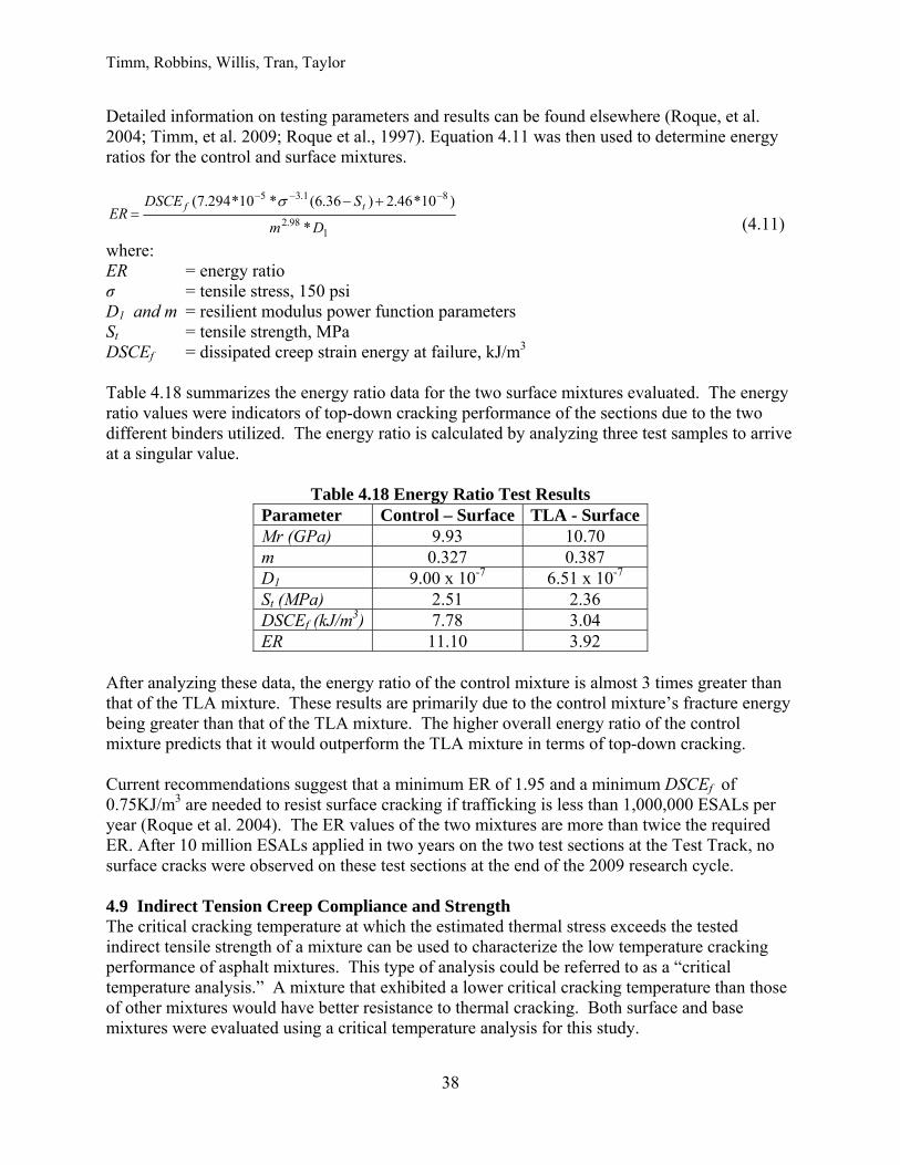
Timm, Robbins, Willis, Tran, Taylor
38
Detailed information on testing parameters and results can be found elsewhere (Roque, et al. 2004; Timm, et al. 2009; Roque et al., 1997). Equation 4.11 was then used to determine energy ratios for the control and surface mixtures.
198.2
81.35
*
)10*46.2)36.6(*10*294.7(
Dm
SDSCEER
tf
(4.11)
where: ER = energy ratio σ = tensile stress, 150 psi D1 and m = resilient modulus power function parameters St = tensile strength, MPa DSCEf = dissipated creep strain energy at failure, kJ/m3 Table 4.18 summarizes the energy ratio data for the two surface mixtures evaluated. The energy ratio values were indicators of top-down cracking performance of the sections due to the two different binders utilized. The energy ratio is calculated by analyzing three test samples to arrive at a singular value.
Table 4.18 Energy Ratio Test Results Parameter Control – Surface TLA - Surface Mr (GPa) 9.93 10.70 m 0.327 0.387 D1 9.00 x 10⁻⁷ 6.51 x 10⁻⁷
St (MPa) 2.51 2.36 DSCEf (kJ/m3) 7.78 3.04 ER 11.10 3.92
After analyzing these data, the energy ratio of the control mixture is almost 3 times greater than that of the TLA mixture. These results are primarily due to the control mixture’s fracture energy being greater than that of the TLA mixture. The higher overall energy ratio of the control mixture predicts that it would outperform the TLA mixture in terms of top-down cracking. Current recommendations suggest that a minimum ER of 1.95 and a minimum DSCEf of 0.75KJ/m3 are needed to resist surface cracking if trafficking is less than 1,000,000 ESALs per year (Roque et al. 2004). The ER values of the two mixtures are more than twice the required ER. After 10 million ESALs applied in two years on the two test sections at the Test Track, no surface cracks were observed on these test sections at the end of the 2009 research cycle. 4.9 Indirect Tension Creep Compliance and Strength The critical cracking temperature at which the estimated thermal stress exceeds the tested indirect tensile strength of a mixture can be used to characterize the low temperature cracking performance of asphalt mixtures. This type of analysis could be referred to as a “critical temperature analysis.” A mixture that exhibited a lower critical cracking temperature than those of other mixtures would have better resistance to thermal cracking. Both surface and base mixtures were evaluated using a critical temperature analysis for this study.
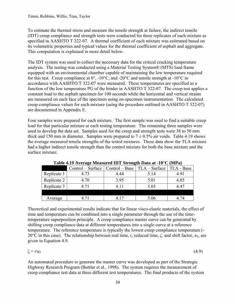
Timm, Robbins, Willis, Tran, Taylor
39
To estimate the thermal stress and measure the tensile strength at failure, the indirect tensile (IDT) creep compliance and strength tests were conducted for three replicates of each mixture as specified in AASHTO T 322-07. A thermal coefficient of each mixture was estimated based on its volumetric properties and typical values for the thermal coefficient of asphalt and aggregate. This computation is explained in more detail below. The IDT system was used to collect the necessary data for the critical cracking temperature analysis. The testing was conducted using a Material Testing System® (MTS) load frame equipped with an environmental chamber capable of maintaining the low temperature required for this test. Creep compliance at 0°, -10°C, and -20°C and tensile strength at -10°C in accordance with AASHTO T 322-07 were measured. These temperatures are specified as a function of the low temperature PG of the binder in AASHTO T 322-07. The creep test applies a constant load to the asphalt specimen for 100 seconds while the horizontal and vertical strains are measured on each face of the specimen using on-specimen instrumentation. The calculated creep compliance values for each mixture (using the procedure outlined in AASHTO T 322-07) are documented in Appendix E. Four samples were prepared for each mixture. The first sample was used to find a suitable creep load for that particular mixture at each testing temperature. The remaining three samples were used to develop the data set. Samples used for the creep and strength tests were 38 to 50 mm thick and 150 mm in diameter. Samples were prepared to 7 ± 0.5% air voids. Table 4.19 shows the average measured tensile strengths of the tested mixtures. These data show the TLA mixture had a higher indirect tensile strength than the control mixture for both the base mixture and the surface mixture.
Table 4.19 Average Measured IDT Strength Data at -10°C (MPa) Control – Surface Control – Base TLA – Surface TLA - Base
Replicate 1 4.73 4.44 5.14 4.91 Replicate 2 4.70 3.95 5.01 4.85 Replicate 3 4.71 4.11 5.03 4.47
Average 4.71 4.17 5.06 4.74
Theoretical and experimental results indicate that for linear visco-elastic materials, the effect of time and temperature can be combined into a single parameter through the use of the time-temperature superposition principle. A creep compliance master curve can be generated by shifting creep compliance data at different temperatures into a single curve at a reference temperature. The reference temperature is typically the lowest creep compliance temperature (-20°C in this case). The relationship between real time, t, reduced time, ζ, and shift factor, aT, are given in Equation 4.9. ζ = t/aT (4.9) An automated procedure to generate the master curve was developed as part of the Strategic Highway Research Program (Buttlar et al., 1998). The system requires the measurement of creep compliance test data at three different test temperatures. The final products of the system
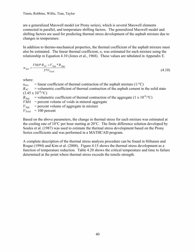
Timm, Robbins, Willis, Tran, Taylor
40
are a generalized Maxwell model (or Prony series), which is several Maxwell elements connected in parallel, and temperature shifting factors. The generalized Maxwell model and shifting factors are used for predicting thermal stress development of the asphalt mixture due to changes in temperature. In addition to thermo-mechanical properties, the thermal coefficient of the asphalt mixture must also be estimated. The linear thermal coefficient, α, was estimated for each mixture using the relationship in Equation 4.10 (Jones et al., 1968). These values are tabulated in Appendix E.
Total
AggAggACmix V
BVBVMA
*3
**
(4.10)
where: αmix = linear coefficient of thermal contraction of the asphalt mixture (1/°C) BAC = volumetric coefficient of thermal contraction of the asphalt cement in the solid state (3.45 x 10⁻⁴/°C) BAgg = volumetric coefficient of thermal contraction of the aggregate (1 x 10⁻⁶/°C) VMA = percent volume of voids in mineral aggregate VAgg = percent volume of aggregate in mixture VTotal = 100 percent Based on the above parameters, the change in thermal stress for each mixture was estimated at the cooling rate of 10°C per hour starting at 20°C. The finite difference solution developed by Soules et al. (1987) was used to estimate the thermal stress development based on the Prony Series coefficients and was performed in a MATHCAD program. A complete description of the thermal stress analysis procedure can be found in Hiltunen and Roque (1994) and Kim et al. (2008). Figure 4.15 shows the thermal stress development as a function of temperature reduction. Table 4.20 shows the critical temperature and time to failure determined at the point where thermal stress exceeds the tensile strength.
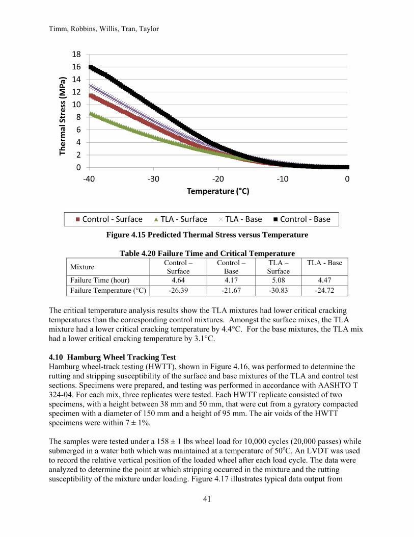
Timm, Robbins, Willis, Tran, Taylor
41
Figure 4.15 Predicted Thermal Stress versus Temperature
Table 4.20 Failure Time and Critical Temperature
Mixture Control – Surface
Control – Base
TLA – Surface
TLA - Base
Failure Time (hour) 4.64 4.17 5.08 4.47 Failure Temperature (°C) -26.39 -21.67 -30.83 -24.72
The critical temperature analysis results show the TLA mixtures had lower critical cracking temperatures than the corresponding control mixtures. Amongst the surface mixes, the TLA mixture had a lower critical cracking temperature by 4.4°C. For the base mixtures, the TLA mix had a lower critical cracking temperature by 3.1°C. 4.10 Hamburg Wheel Tracking Test Hamburg wheel-track testing (HWTT), shown in Figure 4.16, was performed to determine the rutting and stripping susceptibility of the surface and base mixtures of the TLA and control test sections. Specimens were prepared, and testing was performed in accordance with AASHTO T 324-04. For each mix, three replicates were tested. Each HWTT replicate consisted of two specimens, with a height between 38 mm and 50 mm, that were cut from a gyratory compacted specimen with a diameter of 150 mm and a height of 95 mm. The air voids of the HWTT specimens were within 7 ± 1%. The samples were tested under a 158 ± 1 lbs wheel load for 10,000 cycles (20,000 passes) while submerged in a water bath which was maintained at a temperature of 50oC. An LVDT was used to record the relative vertical position of the loaded wheel after each load cycle. The data were analyzed to determine the point at which stripping occurred in the mixture and the rutting susceptibility of the mixture under loading. Figure 4.17 illustrates typical data output from
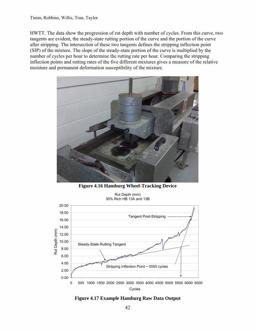
Timm, Robbins, Willis, Tran, Taylor
42
HWTT. The data show the progression of rut depth with number of cycles. From this curve, two tangents are evident, the steady-state rutting portion of the curve and the portion of the curve after stripping. The intersection of these two tangents defines the stripping inflection point (SIP) of the mixture. The slope of the steady-state portion of the curve is multiplied by the number of cycles per hour to determine the rutting rate per hour. Comparing the stripping inflection points and rutting rates of the five different mixtures gives a measure of the relative moisture and permanent deformation susceptibility of the mixture.
Figure 4.16 Hamburg Wheel-Tracking Device
Figure 4.17 Example Hamburg Raw Data Output
Rut Depth (mm)30% Rich HB 13A and 13B
0.00
2.00
4.00
6.00
8.00
10.00
12.00
14.00
16.00
18.00
20.00
0 500 1000 1500 2000 2500 3000 3500 4000 4500 5000 5500 6000 6500
Cycles
Rut
Dep
th (
mm
)
Stripping Inflection Point ~ 5550 cycles
Steady-State Rutting Tangent
Tangent Post-Stripping
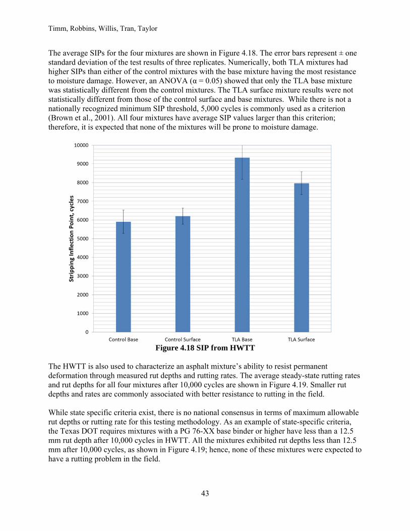
Timm, Robbins, Willis, Tran, Taylor
43
The average SIPs for the four mixtures are shown in Figure 4.18. The error bars represent ± one standard deviation of the test results of three replicates. Numerically, both TLA mixtures had higher SIPs than either of the control mixtures with the base mixture having the most resistance to moisture damage. However, an ANOVA (α = 0.05) showed that only the TLA base mixture was statistically different from the control mixtures. The TLA surface mixture results were not statistically different from those of the control surface and base mixtures. While there is not a nationally recognized minimum SIP threshold, 5,000 cycles is commonly used as a criterion (Brown et al., 2001). All four mixtures have average SIP values larger than this criterion; therefore, it is expected that none of the mixtures will be prone to moisture damage.
Figure 4.18 SIP from HWTT
The HWTT is also used to characterize an asphalt mixture’s ability to resist permanent deformation through measured rut depths and rutting rates. The average steady-state rutting rates and rut depths for all four mixtures after 10,000 cycles are shown in Figure 4.19. Smaller rut depths and rates are commonly associated with better resistance to rutting in the field. While state specific criteria exist, there is no national consensus in terms of maximum allowable rut depths or rutting rate for this testing methodology. As an example of state-specific criteria, the Texas DOT requires mixtures with a PG 76-XX base binder or higher have less than a 12.5 mm rut depth after 10,000 cycles in HWTT. All the mixtures exhibited rut depths less than 12.5 mm after 10,000 cycles, as shown in Figure 4.19; hence, none of these mixtures were expected to have a rutting problem in the field.
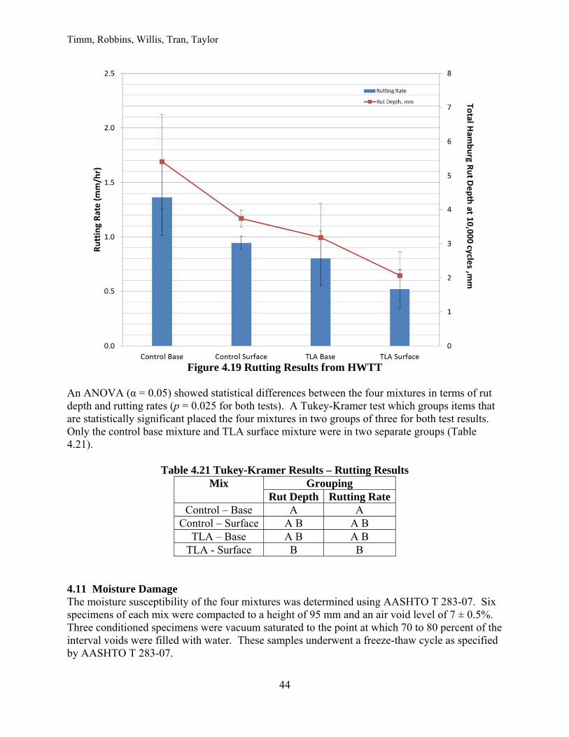
Timm, Robbins, Willis, Tran, Taylor
44
Figure 4.19 Rutting Results from HWTT
An ANOVA (α = 0.05) showed statistical differences between the four mixtures in terms of rut depth and rutting rates (p = 0.025 for both tests). A Tukey-Kramer test which groups items that are statistically significant placed the four mixtures in two groups of three for both test results. Only the control base mixture and TLA surface mixture were in two separate groups (Table 4.21).
Table 4.21 Tukey-Kramer Results – Rutting Results
Mix Grouping Rut Depth Rutting Rate
Control – Base A A Control – Surface A B A B
TLA – Base A B A B TLA - Surface B B
4.11 Moisture Damage The moisture susceptibility of the four mixtures was determined using AASHTO T 283-07. Six specimens of each mix were compacted to a height of 95 mm and an air void level of 7 ± 0.5%. Three conditioned specimens were vacuum saturated to the point at which 70 to 80 percent of the interval voids were filled with water. These samples underwent a freeze-thaw cycle as specified by AASHTO T 283-07.
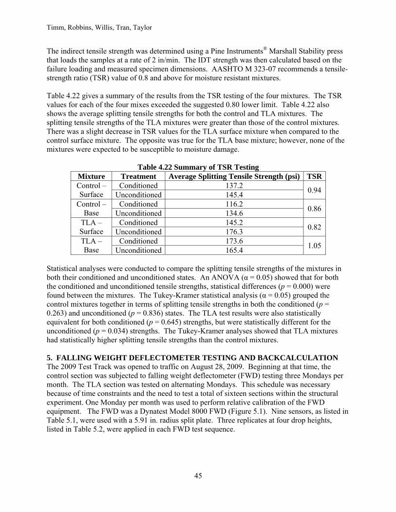
Timm, Robbins, Willis, Tran, Taylor
45
The indirect tensile strength was determined using a Pine Instruments® Marshall Stability press that loads the samples at a rate of 2 in/min. The IDT strength was then calculated based on the failure loading and measured specimen dimensions. AASHTO M 323-07 recommends a tensile-strength ratio (TSR) value of 0.8 and above for moisture resistant mixtures. Table 4.22 gives a summary of the results from the TSR testing of the four mixtures. The TSR values for each of the four mixes exceeded the suggested 0.80 lower limit. Table 4.22 also shows the average splitting tensile strengths for both the control and TLA mixtures. The splitting tensile strengths of the TLA mixtures were greater than those of the control mixtures. There was a slight decrease in TSR values for the TLA surface mixture when compared to the control surface mixture. The opposite was true for the TLA base mixture; however, none of the mixtures were expected to be susceptible to moisture damage.
Table 4.22 Summary of TSR Testing Mixture Treatment Average Splitting Tensile Strength (psi) TSRControl – Surface
Conditioned 137.2 0.94
Unconditioned 145.4 Control –
Base Conditioned 116.2
0.86 Unconditioned 134.6
TLA – Surface
Conditioned 145.2 0.82
Unconditioned 176.3 TLA – Base
Conditioned 173.6 1.05
Unconditioned 165.4 Statistical analyses were conducted to compare the splitting tensile strengths of the mixtures in both their conditioned and unconditioned states. An ANOVA (α = 0.05) showed that for both the conditioned and unconditioned tensile strengths, statistical differences (p = 0.000) were found between the mixtures. The Tukey-Kramer statistical analysis (α = 0.05) grouped the control mixtures together in terms of splitting tensile strengths in both the conditioned (p = 0.263) and unconditioned (p = 0.836) states. The TLA test results were also statistically equivalent for both conditioned (p = 0.645) strengths, but were statistically different for the unconditioned (p = 0.034) strengths. The Tukey-Kramer analyses showed that TLA mixtures had statistically higher splitting tensile strengths than the control mixtures. 5. FALLING WEIGHT DEFLECTOMETER TESTING AND BACKCALCULATION The 2009 Test Track was opened to traffic on August 28, 2009. Beginning at that time, the control section was subjected to falling weight deflectometer (FWD) testing three Mondays per month. The TLA section was tested on alternating Mondays. This schedule was necessary because of time constraints and the need to test a total of sixteen sections within the structural experiment. One Monday per month was used to perform relative calibration of the FWD equipment. The FWD was a Dynatest Model 8000 FWD (Figure 5.1). Nine sensors, as listed in Table 5.1, were used with a 5.91 in. radius split plate. Three replicates at four drop heights, listed in Table 5.2, were applied in each FWD test sequence.
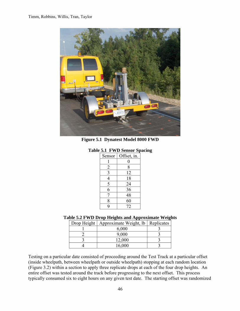
Timm, Robbins, Willis, Tran, Taylor
46
Figure 5.1 Dynatest Model 8000 FWD
Table 5.1 FWD Sensor Spacing
Sensor Offset, in.1 0 2 8 3 12 4 18 5 24 6 36 7 48 8 60 9 72
Table 5.2 FWD Drop Heights and Approximate Weights
Drop Height Approximate Weight, lb Replicates 1 6,000 3 2 9,000 3 3 12,000 3 4 16,000 3
Testing on a particular date consisted of proceeding around the Test Track at a particular offset (inside wheelpath, between wheelpath or outside wheelpath) stopping at each random location (Figure 3.2) within a section to apply three replicate drops at each of the four drop heights. An entire offset was tested around the track before progressing to the next offset. This process typically consumed six to eight hours on any given test date. The starting offset was randomized
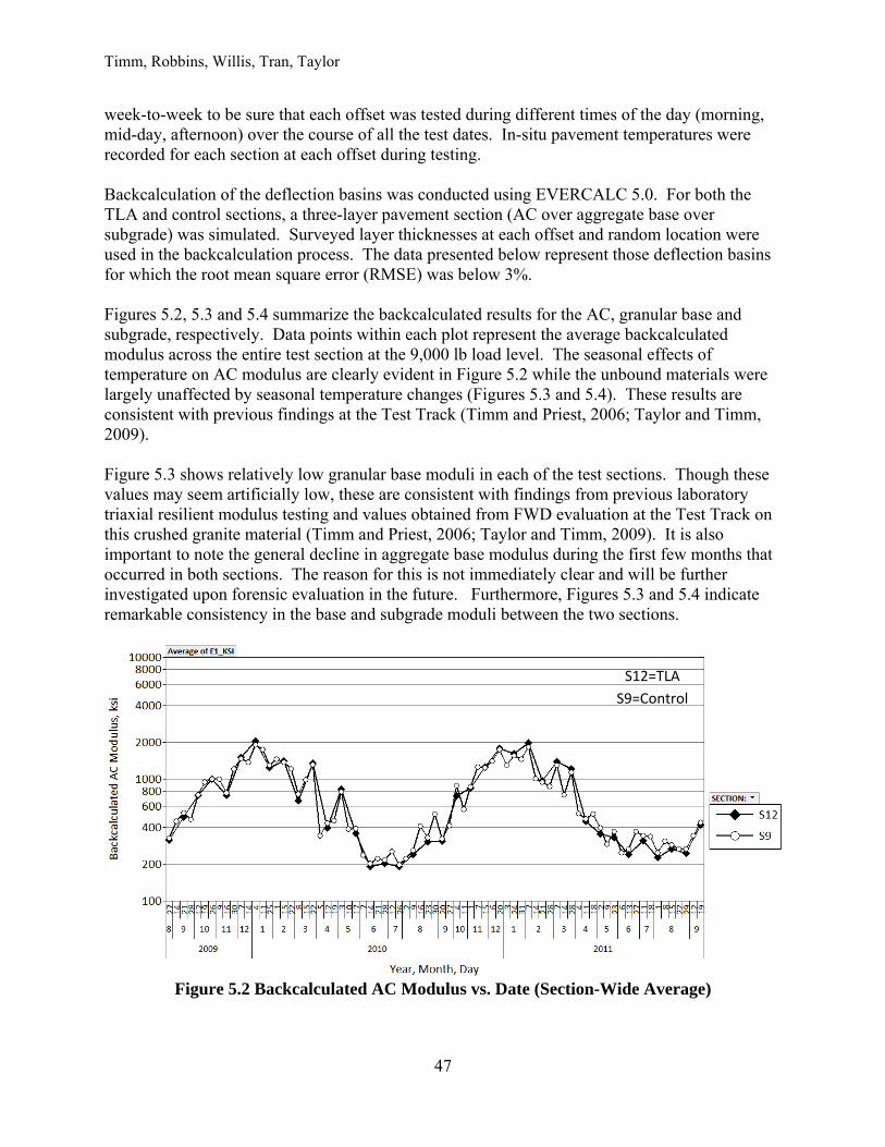
Timm, Robbins, Willis, Tran, Taylor
47
week-to-week to be sure that each offset was tested during different times of the day (morning, mid-day, afternoon) over the course of all the test dates. In-situ pavement temperatures were recorded for each section at each offset during testing. Backcalculation of the deflection basins was conducted using EVERCALC 5.0. For both the TLA and control sections, a three-layer pavement section (AC over aggregate base over subgrade) was simulated. Surveyed layer thicknesses at each offset and random location were used in the backcalculation process. The data presented below represent those deflection basins for which the root mean square error (RMSE) was below 3%. Figures 5.2, 5.3 and 5.4 summarize the backcalculated results for the AC, granular base and subgrade, respectively. Data points within each plot represent the average backcalculated modulus across the entire test section at the 9,000 lb load level. The seasonal effects of temperature on AC modulus are clearly evident in Figure 5.2 while the unbound materials were largely unaffected by seasonal temperature changes (Figures 5.3 and 5.4). These results are consistent with previous findings at the Test Track (Timm and Priest, 2006; Taylor and Timm, 2009). Figure 5.3 shows relatively low granular base moduli in each of the test sections. Though these values may seem artificially low, these are consistent with findings from previous laboratory triaxial resilient modulus testing and values obtained from FWD evaluation at the Test Track on this crushed granite material (Timm and Priest, 2006; Taylor and Timm, 2009). It is also important to note the general decline in aggregate base modulus during the first few months that occurred in both sections. The reason for this is not immediately clear and will be further investigated upon forensic evaluation in the future. Furthermore, Figures 5.3 and 5.4 indicate remarkable consistency in the base and subgrade moduli between the two sections.
Figure 5.2 Backcalculated AC Modulus vs. Date (Section-Wide Average)
S12=TLA
S9=Control
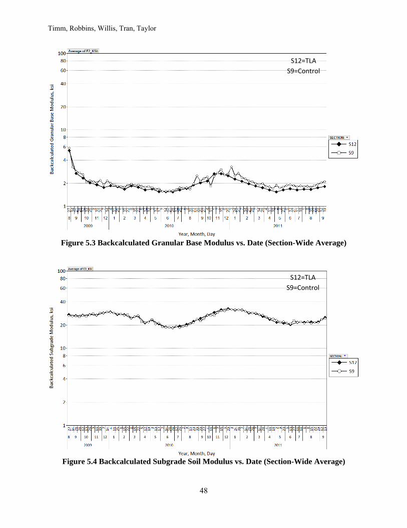
Timm, Robbins, Willis, Tran, Taylor
48
Figure 5.3 Backcalculated Granular Base Modulus vs. Date (Section-Wide Average)
Figure 5.4 Backcalculated Subgrade Soil Modulus vs. Date (Section-Wide Average)
S12=TLA
S9=Control
S12=TLA
S9=Control
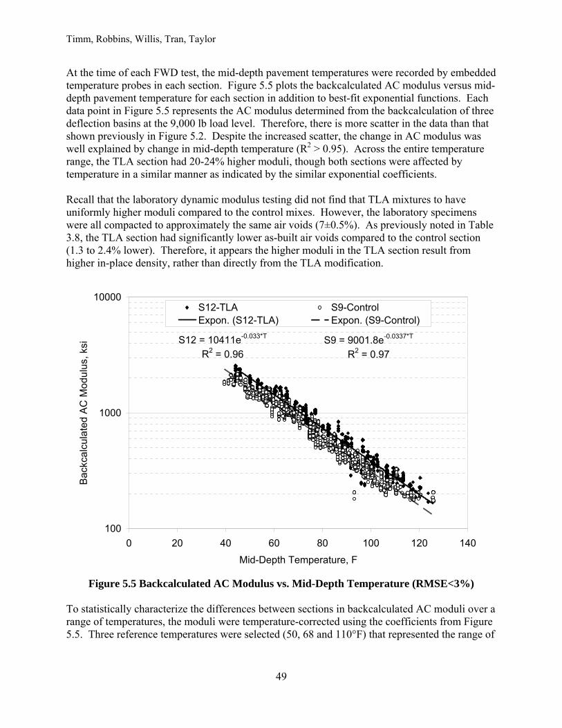
Timm, Robbins, Willis, Tran, Taylor
49
At the time of each FWD test, the mid-depth pavement temperatures were recorded by embedded temperature probes in each section. Figure 5.5 plots the backcalculated AC modulus versus mid-depth pavement temperature for each section in addition to best-fit exponential functions. Each data point in Figure 5.5 represents the AC modulus determined from the backcalculation of three deflection basins at the 9,000 lb load level. Therefore, there is more scatter in the data than that shown previously in Figure 5.2. Despite the increased scatter, the change in AC modulus was well explained by change in mid-depth temperature (R2 > 0.95). Across the entire temperature range, the TLA section had 20-24% higher moduli, though both sections were affected by temperature in a similar manner as indicated by the similar exponential coefficients. Recall that the laboratory dynamic modulus testing did not find that TLA mixtures to have uniformly higher moduli compared to the control mixes. However, the laboratory specimens were all compacted to approximately the same air voids (7±0.5%). As previously noted in Table 3.8, the TLA section had significantly lower as-built air voids compared to the control section (1.3 to 2.4% lower). Therefore, it appears the higher moduli in the TLA section result from higher in-place density, rather than directly from the TLA modification.
Figure 5.5 Backcalculated AC Modulus vs. Mid-Depth Temperature (RMSE<3%)
To statistically characterize the differences between sections in backcalculated AC moduli over a range of temperatures, the moduli were temperature-corrected using the coefficients from Figure 5.5. Three reference temperatures were selected (50, 68 and 110°F) that represented the range of
S12 = 10411e-0.033*T
R2 = 0.96
S9 = 9001.8e-0.0337*T
R2 = 0.97
100
1000
10000
0 20 40 60 80 100 120 140
Mid-Depth Temperature, F
Bac
kcal
cula
ted
AC
Mod
ulus
, ksi
S12-TLA S9-ControlExpon. (S12-TLA) Expon. (S9-Control)
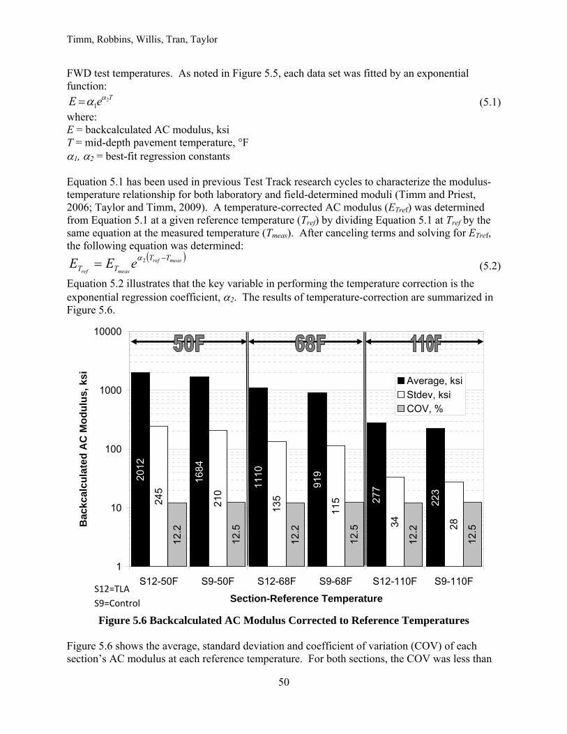
Timm, Robbins, Willis, Tran, Taylor
50
FWD test temperatures. As noted in Figure 5.5, each data set was fitted by an exponential function:
TeE 21
(5.1) where: E = backcalculated AC modulus, ksi T = mid-depth pavement temperature, °F 1, 2 = best-fit regression constants Equation 5.1 has been used in previous Test Track research cycles to characterize the modulus-temperature relationship for both laboratory and field-determined moduli (Timm and Priest, 2006; Taylor and Timm, 2009). A temperature-corrected AC modulus (ETref) was determined from Equation 5.1 at a given reference temperature (Tref) by dividing Equation 5.1 at Tref by the same equation at the measured temperature (Tmeas). After canceling terms and solving for ETref, the following equation was determined:
measref
measref
TTTT eEE 2
(5.2)
Equation 5.2 illustrates that the key variable in performing the temperature correction is the exponential regression coefficient, 2. The results of temperature-correction are summarized in Figure 5.6.
Figure 5.6 Backcalculated AC Modulus Corrected to Reference Temperatures
Figure 5.6 shows the average, standard deviation and coefficient of variation (COV) of each section’s AC modulus at each reference temperature. For both sections, the COV was less than
2012
1684
1110
919
277
223
245
210
135
115
34 28
12.2
12.5
12.2
12.5
12.2
12.5
1
10
100
1000
10000
S12-50F S9-50F S12-68F S9-68F S12-110F S9-110F
Section-Reference Temperature
Bac
kcal
cula
ted
AC
Mo
du
lus,
ksi Average, ksi
Stdev, ksiCOV, %
S12=TLA
S9=Control
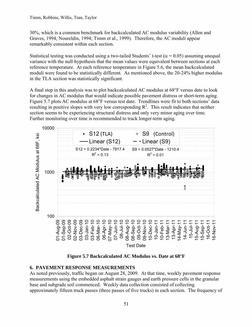
Timm, Robbins, Willis, Tran, Taylor
51
30%, which is a common benchmark for backcalculated AC modulus variability (Allen and Graves, 1994; Noureldin, 1994; Timm et al., 1999). Therefore, the AC moduli appear remarkably consistent within each section. Statistical testing was conducted using a two-tailed Students’ t-test ( = 0.05) assuming unequal variance with the null-hypothesis that the mean values were equivalent between sections at each reference temperature. At each reference temperature in Figure 5.6, the mean backcalculated moduli were found to be statistically different. As mentioned above, the 20-24% higher modulus in the TLA section was statistically significant. A final step in this analysis was to plot backcalculated AC modulus at 68°F versus date to look for changes in AC modulus that would indicate possible pavement distress or short-term aging. Figure 5.7 plots AC modulus at 68°F versus test date. Trendlines were fit to both sections’ data resulting in positive slopes with very low corresponding R2. This result indicates that neither section seems to be experiencing structural distress and only very minor aging over time. Further monitoring over time is recommended to track longer-term aging.
Figure 5.7 Backcalculated AC Modulus vs. Date at 68°F
6. PAVEMENT RESPONSE MEASUREMENTS As noted previously, traffic began on August 28, 2009. At that time, weekly pavement response measurements using the embedded asphalt strain gauges and earth pressure cells in the granular base and subgrade soil commenced. Weekly data collection consisted of collecting approximately fifteen truck passes (three passes of five trucks) in each section. The frequency of
S12 = 0.2234*Date - 7917.4
R2 = 0.13S9 = 0.0527*Date - 1210.4
R2 = 0.01
100
1000
10000
01-A
ug-
0901
-Se
p-09
02-O
ct-0
902
-Nov
-09
03-D
ec-0
903
-Ja
n-10
03-F
eb-
1006
-Ma
r-10
06-A
pr-
1007
-May
-10
07-J
un-
100
8-Ju
l-10
08-A
ug-
1008
-Se
p-10
09-O
ct-1
009
-Nov
-10
10-D
ec-1
010
-Ja
n-11
10-F
eb-
1113
-Ma
r-11
13-A
pr-
1114
-May
-11
14-J
un-
111
5-Ju
l-11
15-A
ug-
1115
-Se
p-11
16-O
ct-1
116
-Nov
-11
Test Date
Ba
ckca
lcu
late
d A
C M
odul
us a
t 68F
, ksi S12 S9
Linear (S12) Linear (S9)(TLA) (Control)
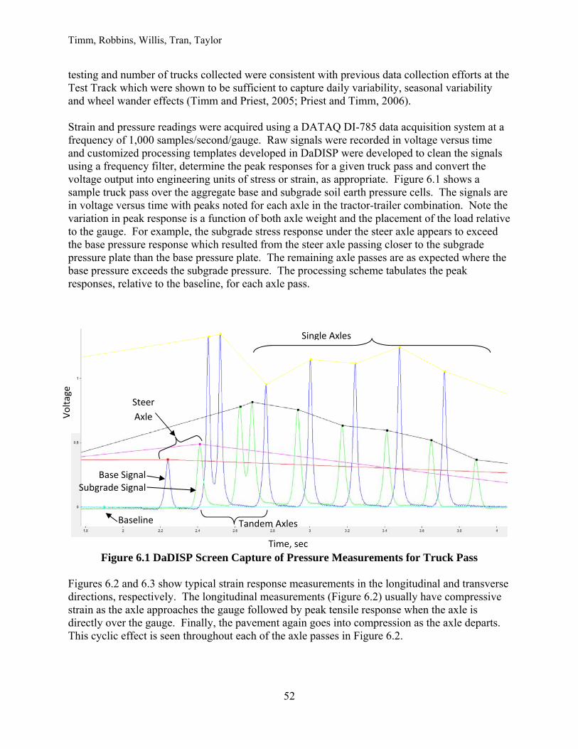
Timm, Robbins, Willis, Tran, Taylor
52
testing and number of trucks collected were consistent with previous data collection efforts at the Test Track which were shown to be sufficient to capture daily variability, seasonal variability and wheel wander effects (Timm and Priest, 2005; Priest and Timm, 2006). Strain and pressure readings were acquired using a DATAQ DI-785 data acquisition system at a frequency of 1,000 samples/second/gauge. Raw signals were recorded in voltage versus time and customized processing templates developed in DaDISP were developed to clean the signals using a frequency filter, determine the peak responses for a given truck pass and convert the voltage output into engineering units of stress or strain, as appropriate. Figure 6.1 shows a sample truck pass over the aggregate base and subgrade soil earth pressure cells. The signals are in voltage versus time with peaks noted for each axle in the tractor-trailer combination. Note the variation in peak response is a function of both axle weight and the placement of the load relative to the gauge. For example, the subgrade stress response under the steer axle appears to exceed the base pressure response which resulted from the steer axle passing closer to the subgrade pressure plate than the base pressure plate. The remaining axle passes are as expected where the base pressure exceeds the subgrade pressure. The processing scheme tabulates the peak responses, relative to the baseline, for each axle pass.
Figure 6.1 DaDISP Screen Capture of Pressure Measurements for Truck Pass Figures 6.2 and 6.3 show typical strain response measurements in the longitudinal and transverse directions, respectively. The longitudinal measurements (Figure 6.2) usually have compressive strain as the axle approaches the gauge followed by peak tensile response when the axle is directly over the gauge. Finally, the pavement again goes into compression as the axle departs. This cyclic effect is seen throughout each of the axle passes in Figure 6.2.
Baseline
Base Signal Subgrade Signal
Steer
Axle
Tandem Axles
Single Axles
Time, sec
Voltage
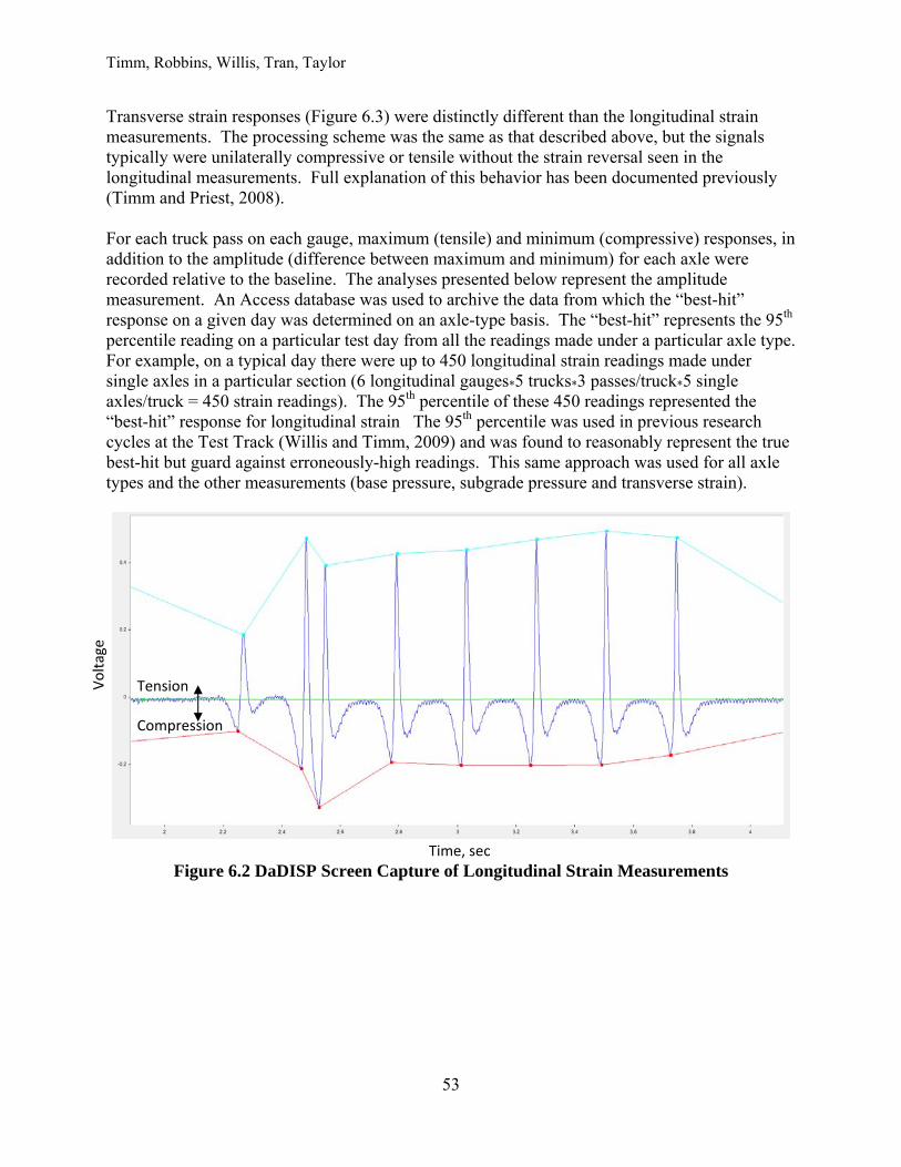
Timm, Robbins, Willis, Tran, Taylor
53
Transverse strain responses (Figure 6.3) were distinctly different than the longitudinal strain measurements. The processing scheme was the same as that described above, but the signals typically were unilaterally compressive or tensile without the strain reversal seen in the longitudinal measurements. Full explanation of this behavior has been documented previously (Timm and Priest, 2008). For each truck pass on each gauge, maximum (tensile) and minimum (compressive) responses, in addition to the amplitude (difference between maximum and minimum) for each axle were recorded relative to the baseline. The analyses presented below represent the amplitude measurement. An Access database was used to archive the data from which the “best-hit” response on a given day was determined on an axle-type basis. The “best-hit” represents the 95th percentile reading on a particular test day from all the readings made under a particular axle type. For example, on a typical day there were up to 450 longitudinal strain readings made under single axles in a particular section (6 longitudinal gauges*5 trucks*3 passes/truck*5 single axles/truck = 450 strain readings). The 95th percentile of these 450 readings represented the “best-hit” response for longitudinal strain The 95th percentile was used in previous research cycles at the Test Track (Willis and Timm, 2009) and was found to reasonably represent the true best-hit but guard against erroneously-high readings. This same approach was used for all axle types and the other measurements (base pressure, subgrade pressure and transverse strain).
Figure 6.2 DaDISP Screen Capture of Longitudinal Strain Measurements
Tension Compression
Time, sec
Voltage
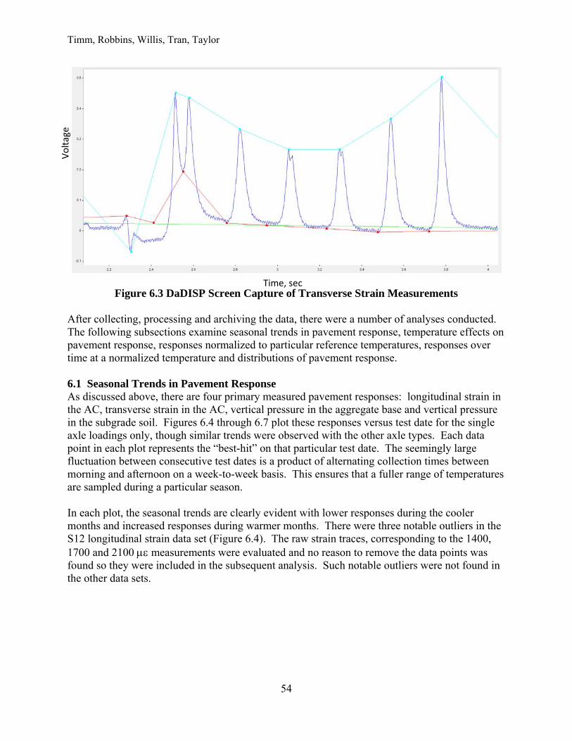
Timm, Robbins, Willis, Tran, Taylor
54
Figure 6.3 DaDISP Screen Capture of Transverse Strain Measurements After collecting, processing and archiving the data, there were a number of analyses conducted. The following subsections examine seasonal trends in pavement response, temperature effects on pavement response, responses normalized to particular reference temperatures, responses over time at a normalized temperature and distributions of pavement response. 6.1 Seasonal Trends in Pavement Response As discussed above, there are four primary measured pavement responses: longitudinal strain in the AC, transverse strain in the AC, vertical pressure in the aggregate base and vertical pressure in the subgrade soil. Figures 6.4 through 6.7 plot these responses versus test date for the single axle loadings only, though similar trends were observed with the other axle types. Each data point in each plot represents the “best-hit” on that particular test date. The seemingly large fluctuation between consecutive test dates is a product of alternating collection times between morning and afternoon on a week-to-week basis. This ensures that a fuller range of temperatures are sampled during a particular season. In each plot, the seasonal trends are clearly evident with lower responses during the cooler months and increased responses during warmer months. There were three notable outliers in the S12 longitudinal strain data set (Figure 6.4). The raw strain traces, corresponding to the 1400, 1700 and 2100 measurements were evaluated and no reason to remove the data points was found so they were included in the subsequent analysis. Such notable outliers were not found in the other data sets.
Time, sec
Voltage
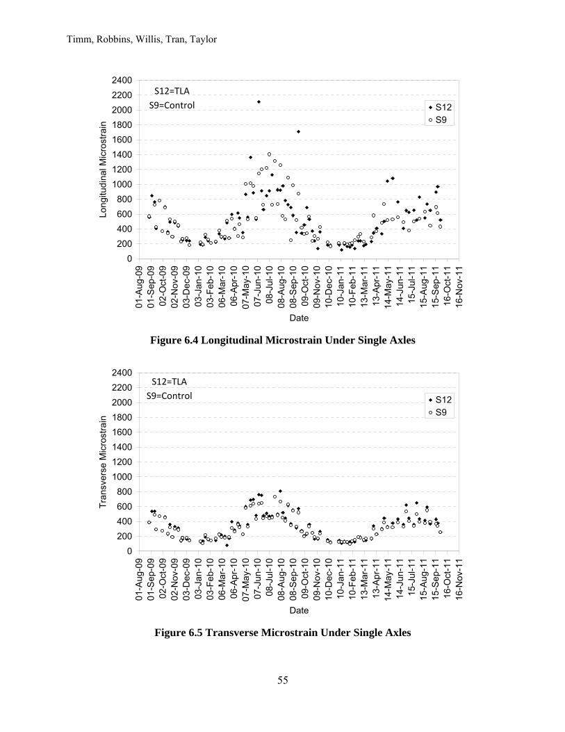
Timm, Robbins, Willis, Tran, Taylor
55
Figure 6.4 Longitudinal Microstrain Under Single Axles
Figure 6.5 Transverse Microstrain Under Single Axles
0
200
400
600
800
1000
1200
1400
1600
1800
2000
2200
2400
01-
Aug
-09
01-
Sep
-09
02-O
ct-0
902
-Nov
-09
03-D
ec-0
903
-Jan
-10
03-F
eb-
1006
-Mar
-10
06-A
pr-1
00
7-M
ay-1
007
-Jun
-10
08-J
ul-1
00
8-A
ug-1
00
8-S
ep-1
009
-Oct
-10
09-N
ov-1
010
-Dec
-10
10-J
an-1
110
-Fe
b-11
13-M
ar-1
113
-Apr
-11
14-
May
-11
14-J
un-1
115
-Jul
-11
15-
Aug
-11
15-
Sep
-11
16-O
ct-1
116
-Nov
-11
Date
Long
itud
ina
l Mic
rost
rain
S12S9
0
200
400
600
800
1000
1200
1400
1600
1800
2000
2200
2400
01-A
ug-
0901
-Se
p-09
02-
Oct
-09
02-N
ov-0
903
-Dec
-09
03-
Jan-
1003
-Fe
b-10
06-M
ar-
100
6-A
pr-
1007
-Ma
y-1
00
7-Ju
n-10
08-J
ul-1
008
-Au
g-10
08-S
ep-
100
9-O
ct-1
009
-Nov
-10
10-D
ec-1
01
0-Ja
n-11
10-F
eb-
1113
-Ma
r-11
13-
Ap
r-11
14-M
ay-
11
14-
Jun-
1115
-Jul
-11
15-A
ug-
1115
-Se
p-11
16-
Oct
-11
16-N
ov-1
1
Date
Tra
nsve
rse
Mic
rost
rain
S12S9
S12=TLA
S9=Control
S12=TLA
S9=Control
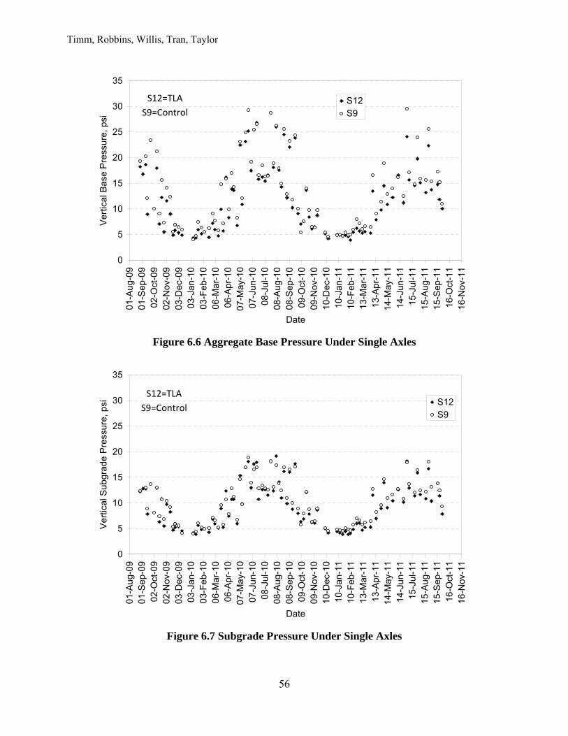
Timm, Robbins, Willis, Tran, Taylor
56
Figure 6.6 Aggregate Base Pressure Under Single Axles
Figure 6.7 Subgrade Pressure Under Single Axles
0
5
10
15
20
25
30
35
01-
Aug
-09
01-
Sep
-09
02-O
ct-0
902
-Nov
-09
03-D
ec-0
90
3-Ja
n-10
03-F
eb-
1006
-Mar
-10
06-A
pr-1
00
7-M
ay-1
00
7-Ju
n-10
08-J
ul-1
00
8-A
ug-1
00
8-S
ep-1
009
-Oct
-10
09-N
ov-1
010
-Dec
-10
10-
Jan-
1110
-Fe
b-11
13-M
ar-1
113
-Apr
-11
14-
May
-11
14-
Jun-
1115
-Jul
-11
15-
Aug
-11
15-
Sep
-11
16-O
ct-1
116
-Nov
-11
Date
Ver
tical
Bas
e P
ress
ure,
psi
S12S9
0
5
10
15
20
25
30
35
01-A
ug-
0901
-Se
p-09
02-
Oct
-09
02-N
ov-0
903
-Dec
-09
03-
Jan-
1003
-Fe
b-10
06-M
ar-
100
6-A
pr-
1007
-Ma
y-1
00
7-Ju
n-10
08-J
ul-1
008
-Au
g-10
08-S
ep-
100
9-O
ct-1
009
-Nov
-10
10-D
ec-1
01
0-Ja
n-11
10-F
eb-
1113
-Ma
r-11
13-
Ap
r-11
14-M
ay-
11
14-
Jun-
1115
-Jul
-11
15-A
ug-
1115
-Se
p-11
16-
Oct
-11
16-N
ov-1
1
Date
Ver
tical
Sub
grad
e P
ress
ure,
psi S12
S9
S12=TLA
S9=Control
S12=TLA
S9=Control
Timm, Robbins, Willis, Tran, Taylor
57
6.2 Pavement Response vs. Temperature The data presented in Figures 6.4 through 6.7 were the best-hit pavement responses on a particular test date. These data were replotted in Figures 6.8 through 6.11 against their corresponding mid-depth pavement temperature. Exponential regression equations, of the form shown in Equation 6.1 and much like those determined for the backcalculated AC moduli, were best-fit to each data set in Figures 6.8 through 6.11 representing single axles. Additional equations were developed for each of the axle types, the results of which are presented in Table 6.1. In total, 24 sets of regression parameters were determined (2 sections x 4 responses x 3 axle types = 24). For the control section, all R2 values were above 76%. For the TLA section, all but one response (longitudinal strain under steer axles) were above 70%. Generally speaking, the longitudinal strain data had poorer R2 than any of the other responses which was likely due to gauge functionality rather than section performance since the other responses had relatively less data scatter. In fact, the R2 corresponding to the transverse strain, base pressure and subgrade pressure were remarkably high at 90%, 97% and 98% respectively.
(6.1) where: k1,k2 = regression coefficients T = mid-depth pavement temperature (°F) Figures 6.8 through 6.11 show the same general trend in that at lower temperatures the curves for each section tend to converge, while at higher temperatures the TLA section appears to have lower pavement response. One may expect that the TLA strains should have been lower at all temperatures since the backcalculated moduli were higher at all temperatures. Theoretically, however, there is a negative power function relationship between strain and modulus. This means that a 20% difference in modulus at the highest temperature (lowest moduli) has a bigger impact on strain than a 20% difference in modulus at the lowest temperature (highest moduli). Therefore, it makes sense that it would be more difficult to discern differences at the lower temperatures. The statistical differences are quantified below.
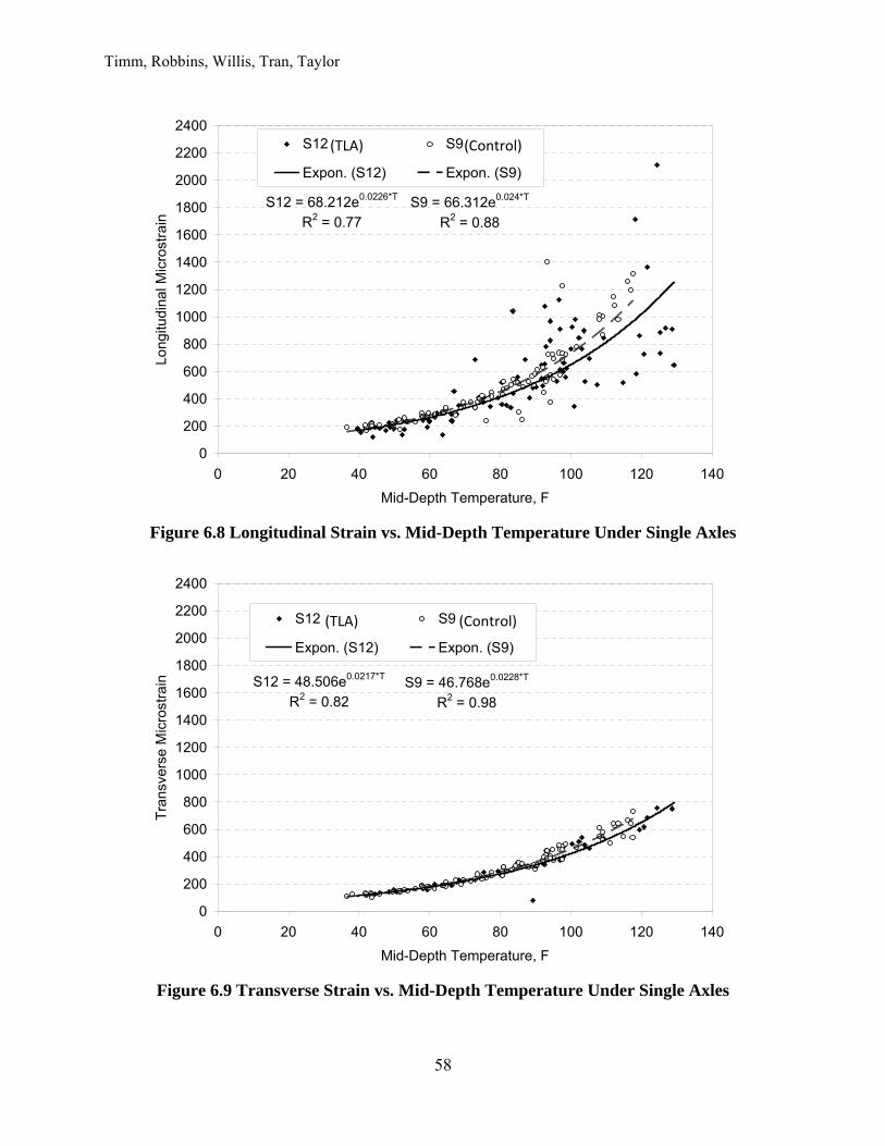
Timm, Robbins, Willis, Tran, Taylor
58
Figure 6.8 Longitudinal Strain vs. Mid-Depth Temperature Under Single Axles
Figure 6.9 Transverse Strain vs. Mid-Depth Temperature Under Single Axles
S12 = 68.212e0.0226*T
R2 = 0.77
S9 = 66.312e0.024*T
R2 = 0.88
0
200
400
600
800
1000
1200
1400
1600
1800
2000
2200
2400
0 20 40 60 80 100 120 140
Mid-Depth Temperature, F
Long
itudi
nal M
icro
stra
inS12 S9
Expon. (S12) Expon. (S9)
S12 = 48.506e0.0217*T
R2 = 0.82S9 = 46.768e0.0228*T
R2 = 0.98
0
200
400
600
800
1000
1200
1400
1600
1800
2000
2200
2400
0 20 40 60 80 100 120 140
Mid-Depth Temperature, F
Tra
nsv
erse
Mic
rost
rain
S12 S9
Expon. (S12) Expon. (S9)
(TLA) (Control)
(TLA) (Control)
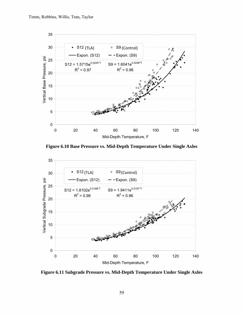
Timm, Robbins, Willis, Tran, Taylor
59
Figure 6.10 Base Pressure vs. Mid-Depth Temperature Under Single Axles
Figure 6.11 Subgrade Pressure vs. Mid-Depth Temperature Under Single Axles
S12 = 1.5715e0.0225*T
R2 = 0.97
S9 = 1.6041e0.0248*T
R2 = 0.96
0
5
10
15
20
25
30
35
0 20 40 60 80 100 120 140
Mid-Depth Temperature, F
Ver
tical
Bas
e P
ress
ure,
psi
S12 S9
Expon. (S12) Expon. (S9)
S12 = 1.8102e0.0188*T
R2 = 0.98
S9 = 1.9411e0.0197*T
R2 = 0.96
0
5
10
15
20
25
30
35
0 20 40 60 80 100 120 140
Mid-Depth Temperature, F
Ve
rtic
al S
ub
gra
de
Pre
ssu
re, p
si
S12 S9
Expon. (S12) Expon. (S9)
(TLA) (Control)
(TLA) (Control)
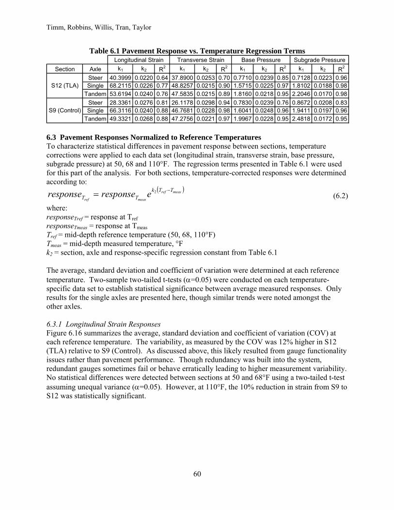
Timm, Robbins, Willis, Tran, Taylor
60
Table 6.1 Pavement Response vs. Temperature Regression Terms
6.3 Pavement Responses Normalized to Reference Temperatures To characterize statistical differences in pavement response between sections, temperature corrections were applied to each data set (longitudinal strain, transverse strain, base pressure, subgrade pressure) at 50, 68 and 110°F. The regression terms presented in Table 6.1 were used for this part of the analysis. For both sections, temperature-corrected responses were determined according to:
measref
measref
TTkTT eresponseresponse 2
(6.2)
where: responseTref = response at Tref responseTmeas = response at Tmeas Tref = mid-depth reference temperature (50, 68, 110°F) Tmeas = mid-depth measured temperature, °F k2 = section, axle and response-specific regression constant from Table 6.1 The average, standard deviation and coefficient of variation were determined at each reference temperature. Two-sample two-tailed t-tests (=0.05) were conducted on each temperature-specific data set to establish statistical significance between average measured responses. Only results for the single axles are presented here, though similar trends were noted amongst the other axles. 6.3.1 Longitudinal Strain Responses Figure 6.16 summarizes the average, standard deviation and coefficient of variation (COV) at each reference temperature. The variability, as measured by the COV was 12% higher in S12 (TLA) relative to S9 (Control). As discussed above, this likely resulted from gauge functionality issues rather than pavement performance. Though redundancy was built into the system, redundant gauges sometimes fail or behave erratically leading to higher measurement variability. No statistical differences were detected between sections at 50 and 68°F using a two-tailed t-test assuming unequal variance (=0.05). However, at 110°F, the 10% reduction in strain from S9 to S12 was statistically significant.
Section Axle k1 k2 R2 k1 k2 R2 k1 k2 R2 k1 k2 R2
Steer 40.3999 0.0220 0.64 37.8900 0.0253 0.70 0.7710 0.0239 0.85 0.7128 0.0223 0.96Single 68.2115 0.0226 0.77 48.8257 0.0215 0.90 1.5715 0.0225 0.97 1.8102 0.0188 0.98
Tandem 53.6194 0.0240 0.76 47.5835 0.0215 0.89 1.8160 0.0218 0.95 2.2046 0.0170 0.98
Steer 28.3361 0.0276 0.81 26.1178 0.0298 0.94 0.7830 0.0239 0.76 0.8672 0.0208 0.83Single 66.3116 0.0240 0.88 46.7681 0.0228 0.98 1.6041 0.0248 0.96 1.9411 0.0197 0.96
Tandem 49.3321 0.0268 0.88 47.2756 0.0221 0.97 1.9967 0.0228 0.95 2.4818 0.0172 0.95
Base Pressure Subgrade Pressure
S12 (TLA)
S9 (Control)
Longitudinal Strain Transverse Strain
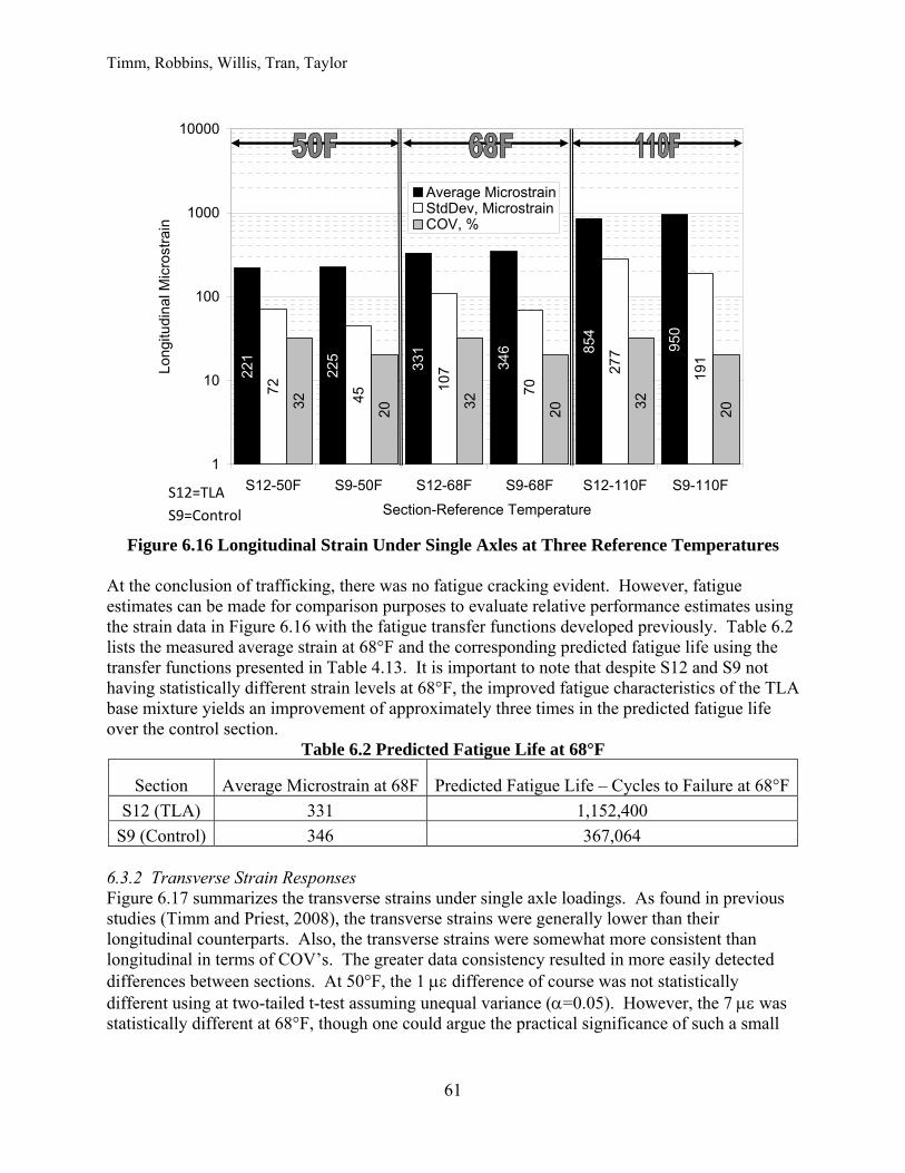
Timm, Robbins, Willis, Tran, Taylor
61
Figure 6.16 Longitudinal Strain Under Single Axles at Three Reference Temperatures
At the conclusion of trafficking, there was no fatigue cracking evident. However, fatigue estimates can be made for comparison purposes to evaluate relative performance estimates using the strain data in Figure 6.16 with the fatigue transfer functions developed previously. Table 6.2 lists the measured average strain at 68°F and the corresponding predicted fatigue life using the transfer functions presented in Table 4.13. It is important to note that despite S12 and S9 not having statistically different strain levels at 68°F, the improved fatigue characteristics of the TLA base mixture yields an improvement of approximately three times in the predicted fatigue life over the control section.
Table 6.2 Predicted Fatigue Life at 68°F
Section Average Microstrain at 68F Predicted Fatigue Life – Cycles to Failure at 68°F
S12 (TLA) 331 1,152,400
S9 (Control) 346 367,064 6.3.2 Transverse Strain Responses Figure 6.17 summarizes the transverse strains under single axle loadings. As found in previous studies (Timm and Priest, 2008), the transverse strains were generally lower than their longitudinal counterparts. Also, the transverse strains were somewhat more consistent than longitudinal in terms of COV’s. The greater data consistency resulted in more easily detected differences between sections. At 50°F, the 1 difference of course was not statistically different using at two-tailed t-test assuming unequal variance (=0.05). However, the 7 was statistically different at 68°F, though one could argue the practical significance of such a small
221
225
331 34
6 854 950
72
45
107
70
277
191
32
20 32
20 32
20
1
10
100
1000
10000
S12-50F S9-50F S12-68F S9-68F S12-110F S9-110F
Section-Reference Temperature
Lon
gitu
din
al M
icro
stra
in
Average MicrostrainStdDev, MicrostrainCOV, %
S12=TLA
S9=Control
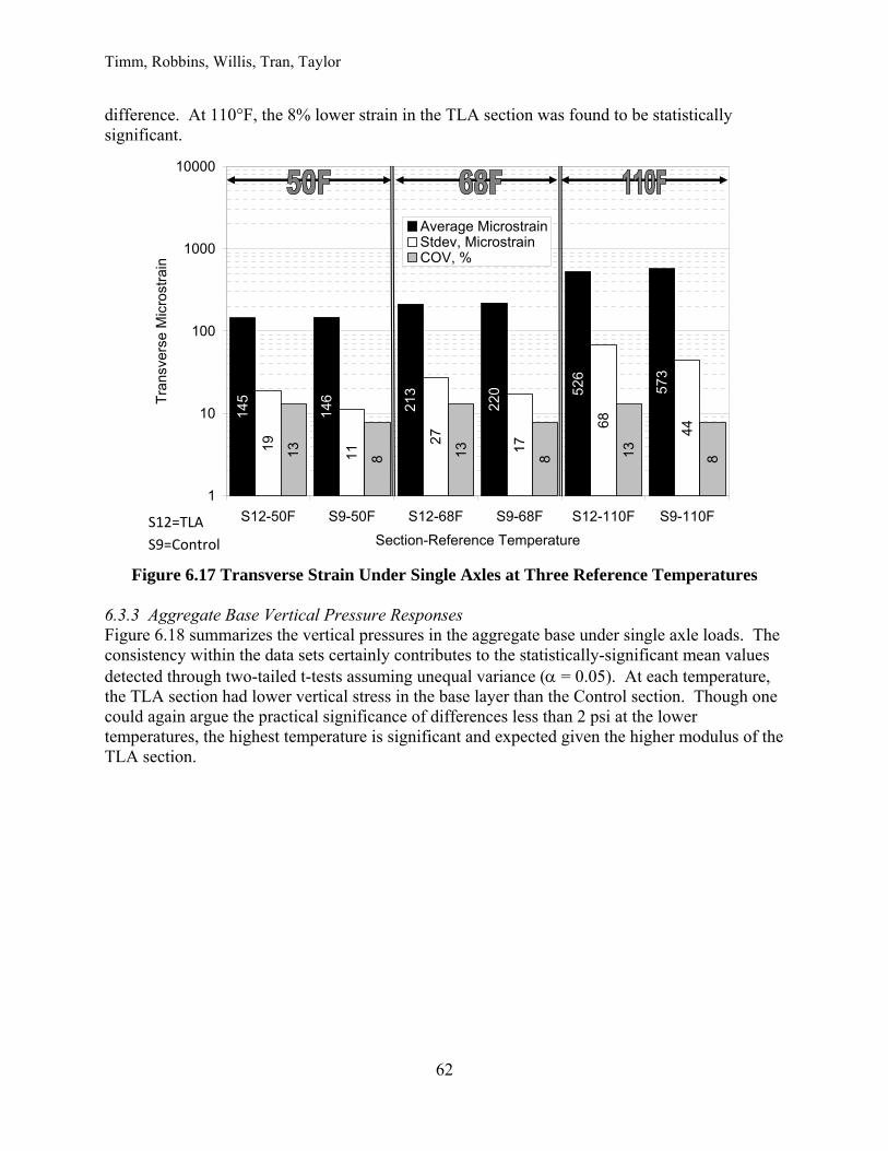
Timm, Robbins, Willis, Tran, Taylor
62
difference. At 110°F, the 8% lower strain in the TLA section was found to be statistically significant.
Figure 6.17 Transverse Strain Under Single Axles at Three Reference Temperatures
6.3.3 Aggregate Base Vertical Pressure Responses Figure 6.18 summarizes the vertical pressures in the aggregate base under single axle loads. The consistency within the data sets certainly contributes to the statistically-significant mean values detected through two-tailed t-tests assuming unequal variance ( = 0.05). At each temperature, the TLA section had lower vertical stress in the base layer than the Control section. Though one could again argue the practical significance of differences less than 2 psi at the lower temperatures, the highest temperature is significant and expected given the higher modulus of the TLA section.
145
146 21
3
220 5
26 573
19
11 2
7
17
68 44
13 8 13 8 13 8
1
10
100
1000
10000
S12-50F S9-50F S12-68F S9-68F S12-110F S9-110F
Section-Reference Temperature
Tra
nsve
rse
Mic
rost
rain
Average MicrostrainStdev, MicrostrainCOV, %
S12=TLA
S9=Control
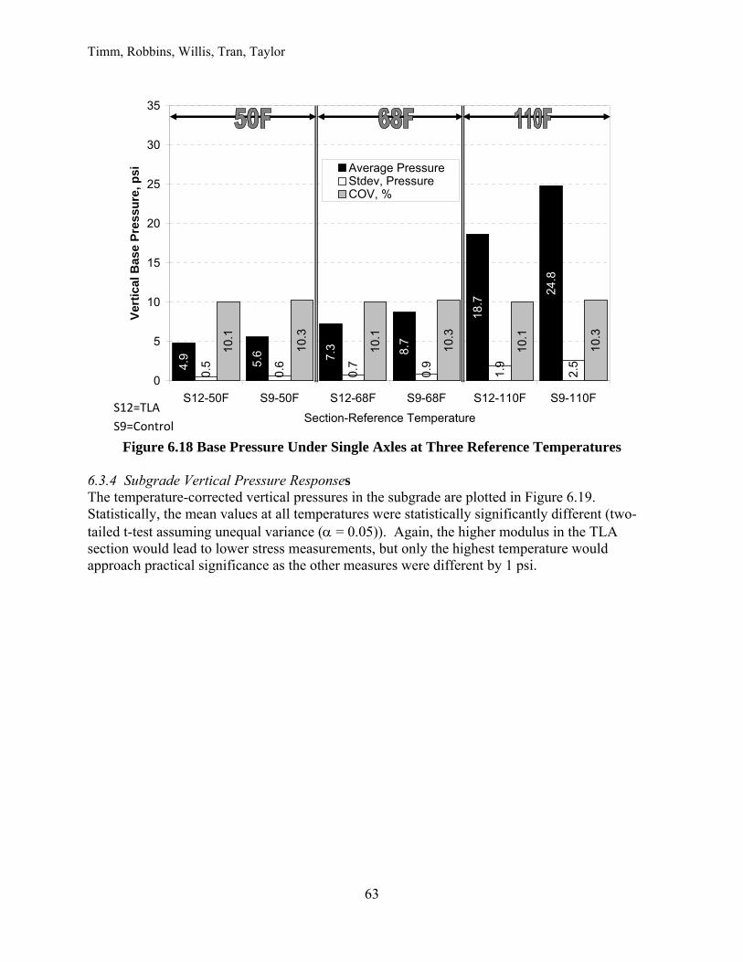
Timm, Robbins, Willis, Tran, Taylor
63
Figure 6.18 Base Pressure Under Single Axles at Three Reference Temperatures
6.3.4 Subgrade Vertical Pressure Responses The temperature-corrected vertical pressures in the subgrade are plotted in Figure 6.19. Statistically, the mean values at all temperatures were statistically significantly different (two-tailed t-test assuming unequal variance ( = 0.05)). Again, the higher modulus in the TLA section would lead to lower stress measurements, but only the highest temperature would approach practical significance as the other measures were different by 1 psi.
4.9 5.6 7.3 8.7
18.7
24.8
0.5
0.6
0.7
0.9
1.9
2.5
10.
1
10.
3
10.
1
10.
3
10.
1
10.
3
0
5
10
15
20
25
30
35
S12-50F S9-50F S12-68F S9-68F S12-110F S9-110F
Section-Reference Temperature
Ver
tica
l Bas
e P
ress
ure
, ps
i Average PressureStdev, PressureCOV, %
S12=TLA
S9=Control
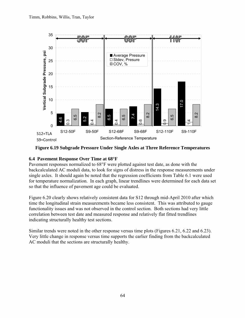
Timm, Robbins, Willis, Tran, Taylor
64
Figure 6.19 Subgrade Pressure Under Single Axles at Three Reference Temperatures
6.4 Pavement Response Over Time at 68°F Pavement responses normalized to 68°F were plotted against test date, as done with the backcalculated AC moduli data, to look for signs of distress in the response measurements under single axles. It should again be noted that the regression coefficients from Table 6.1 were used for temperature normalization. In each graph, linear trendlines were determined for each data set so that the influence of pavement age could be evaluated. Figure 6.20 clearly shows relatively consistent data for S12 through mid-April 2010 after which time the longitudinal strain measurements became less consistent. This was attributed to gauge functionality issues and was not observed in the control section. Both sections had very little correlation between test date and measured response and relatively flat fitted trendlines indicating structurally healthy test sections. Similar trends were noted in the other response versus time plots (Figures 6.21, 6.22 and 6.23). Very little change in response versus time supports the earlier finding from the backcalculated AC moduli that the sections are structurally healthy.
4.6
5.2 6.5 7.
4
14.3 17
.0
0.3
0.4
0.4
0.6
0.9
1.4
6.5 8.
2
6.5 8.
2
6.5 8.
2
0
5
10
15
20
25
30
35
S12-50F S9-50F S12-68F S9-68F S12-110F S9-110F
Section-Reference Temperature
Ver
tica
l Su
bg
rad
e P
ress
ure
, ps
i
Average PressureStdev, PresureCOV, %
S12=TLA
S9=Control
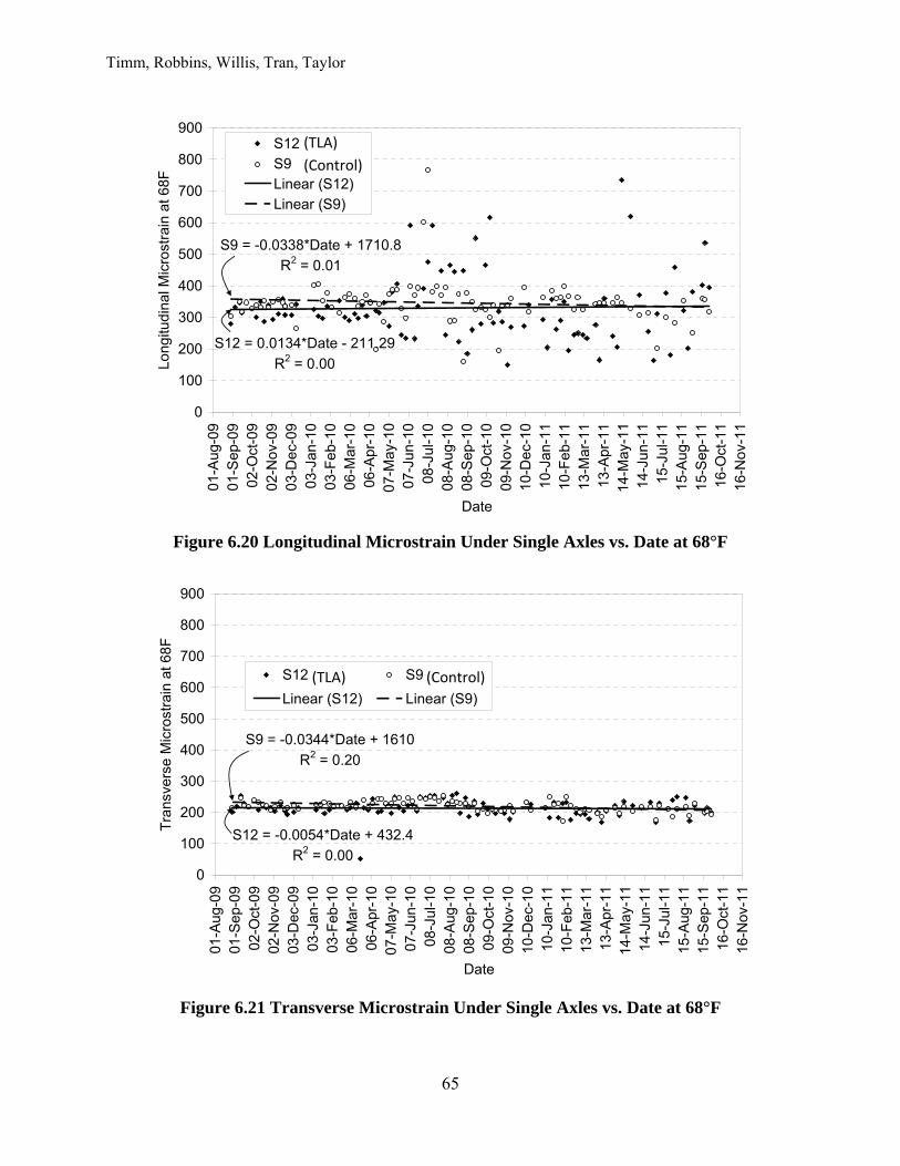
Timm, Robbins, Willis, Tran, Taylor
65
Figure 6.20 Longitudinal Microstrain Under Single Axles vs. Date at 68°F
Figure 6.21 Transverse Microstrain Under Single Axles vs. Date at 68°F
S12 = 0.0134*Date - 211.29
R2 = 0.00
S9 = -0.0338*Date + 1710.8
R2 = 0.01
0
100
200
300
400
500
600
700
800
900
01-
Aug
-09
01-
Sep
-09
02-O
ct-0
902
-Nov
-09
03-D
ec-0
90
3-Ja
n-10
03-F
eb-
1006
-Mar
-10
06-A
pr-1
00
7-M
ay-1
00
7-Ju
n-10
08-J
ul-1
00
8-A
ug-1
00
8-S
ep-1
009
-Oct
-10
09-N
ov-1
010
-Dec
-10
10-
Jan-
1110
-Fe
b-11
13-M
ar-1
113
-Apr
-11
14-
May
-11
14-
Jun-
1115
-Jul
-11
15-
Aug
-11
15-
Sep
-11
16-O
ct-1
116
-Nov
-11
Date
Long
itud
ina
l Mic
rost
rain
at 6
8FS12S9Linear (S12)Linear (S9)
S12 = -0.0054*Date + 432.4
R2 = 0.00
S9 = -0.0344*Date + 1610
R2 = 0.20
0
100
200
300
400
500
600
700
800
900
01-A
ug-0
901
-Sep
-09
02-O
ct-0
902
-Nov
-09
03-D
ec-0
903
-Jan
-10
03-
Feb
-10
06-
Mar
-10
06-A
pr-
10
07-M
ay-
1007
-Jun
-10
08-
Jul-1
008
-Aug
-10
08-S
ep-1
009
-Oct
-10
09-N
ov-1
010
-Dec
-10
10-J
an-1
11
0-F
eb-1
11
3-M
ar-1
113
-Ap
r-1
114
-Ma
y-11
14-J
un-1
11
5-Ju
l-11
15-A
ug-1
115
-Sep
-11
16-O
ct-1
116
-Nov
-11
Date
Tra
nsve
rse
Mic
rost
rain
at 6
8F
S12 S9
Linear (S12) Linear (S9)
(TLA)
(Control)
(TLA) (Control)
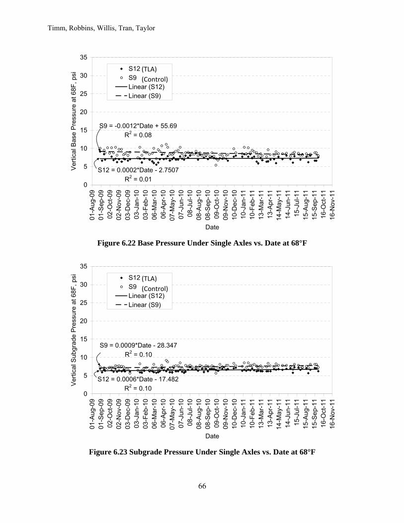
Timm, Robbins, Willis, Tran, Taylor
66
Figure 6.22 Base Pressure Under Single Axles vs. Date at 68°F
Figure 6.23 Subgrade Pressure Under Single Axles vs. Date at 68°F
S12 = 0.0002*Date - 2.7507
R2 = 0.01
S9 = -0.0012*Date + 55.69
R2 = 0.08
0
5
10
15
20
25
30
35
01-
Aug
-09
01-
Sep
-09
02-O
ct-0
902
-Nov
-09
03-D
ec-0
90
3-Ja
n-10
03-F
eb-
1006
-Mar
-10
06-A
pr-1
00
7-M
ay-1
00
7-Ju
n-10
08-J
ul-1
00
8-A
ug-1
00
8-S
ep-1
009
-Oct
-10
09-N
ov-1
010
-Dec
-10
10-
Jan-
1110
-Fe
b-11
13-M
ar-1
113
-Apr
-11
14-
May
-11
14-
Jun-
1115
-Jul
-11
15-
Aug
-11
15-
Sep
-11
16-O
ct-1
116
-Nov
-11
Date
Ver
tical
Bas
e P
ress
ure
at 6
8F,
psi S12
S9Linear (S12)Linear (S9)
S12 = 0.0006*Date - 17.482
R2 = 0.10
S9 = 0.0009*Date - 28.347
R2 = 0.10
0
5
10
15
20
25
30
35
01-A
ug-
0901
-Se
p-09
02-
Oct
-09
02-N
ov-0
903
-Dec
-09
03-
Jan-
1003
-Fe
b-10
06-M
ar-
100
6-A
pr-
1007
-Ma
y-1
00
7-Ju
n-10
08-J
ul-1
008
-Au
g-10
08-S
ep-
100
9-O
ct-1
009
-Nov
-10
10-D
ec-1
01
0-Ja
n-11
10-F
eb-
1113
-Ma
r-11
13-
Ap
r-11
14-M
ay-
11
14-
Jun-
1115
-Jul
-11
15-A
ug-
1115
-Se
p-11
16-
Oct
-11
16-N
ov-1
1
Date
Ver
tica
l Su
bgra
de P
ress
ure
at 6
8F
, psi S12
S9Linear (S12)Linear (S9)
(TLA)
(Control)
(TLA)
(Control)
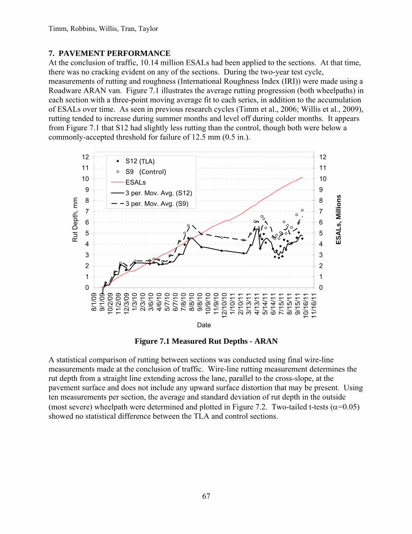
Timm, Robbins, Willis, Tran, Taylor
67
7. PAVEMENT PERFORMANCE At the conclusion of traffic, 10.14 million ESALs had been applied to the sections. At that time, there was no cracking evident on any of the sections. During the two-year test cycle, measurements of rutting and roughness (International Roughness Index (IRI)) were made using a Roadware ARAN van. Figure 7.1 illustrates the average rutting progression (both wheelpaths) in each section with a three-point moving average fit to each series, in addition to the accumulation of ESALs over time. As seen in previous research cycles (Timm et al., 2006; Willis et al., 2009), rutting tended to increase during summer months and level off during colder months. It appears from Figure 7.1 that S12 had slightly less rutting than the control, though both were below a commonly-accepted threshold for failure of 12.5 mm (0.5 in.).
Figure 7.1 Measured Rut Depths - ARAN
A statistical comparison of rutting between sections was conducted using final wire-line measurements made at the conclusion of traffic. Wire-line rutting measurement determines the rut depth from a straight line extending across the lane, parallel to the cross-slope, at the pavement surface and does not include any upward surface distortion that may be present. Using ten measurements per section, the average and standard deviation of rut depth in the outside (most severe) wheelpath were determined and plotted in Figure 7.2. Two-tailed t-tests (=0.05) showed no statistical difference between the TLA and control sections.
0
1
2
3
4
5
6
7
8
9
10
11
12
8/1
/09
9/1
/09
10/2
/09
11/2
/09
12/3
/09
1/3
/10
2/3
/10
3/6
/10
4/6
/10
5/7
/10
6/7
/10
7/8
/10
8/8
/10
9/8
/10
10/9
/10
11/9
/10
12/
10/1
01/
10/1
12/
10/1
13/
13/1
14/
13/1
15/
14/1
16/
14/1
17/
15/1
18/
15/1
19/
15/1
11
0/16
/11
11/
16/1
1
Date
Ru
t De
pth,
mm
0
1
2
3
4
5
6
7
8
9
10
11
12
ES
AL
s, M
illio
ns
S12
S9
ESALs
3 per. Mov. Avg. (S12)
3 per. Mov. Avg. (S9)
(TLA)
(Control)
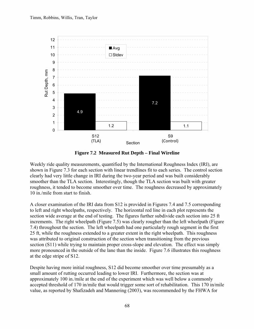
Timm, Robbins, Willis, Tran, Taylor
68
Figure 7.2 Measured Rut Depth – Final Wireline
Weekly ride quality measurements, quantified by the International Roughness Index (IRI), are shown in Figure 7.3 for each section with linear trendlines fit to each series. The control section clearly had very little change in IRI during the two-year period and was built considerably smoother than the TLA section. Interestingly, though the TLA section was built with greater roughness, it tended to become smoother over time. The roughness decreased by approximately 10 in./mile from start to finish. A closer examination of the IRI data from S12 is provided in Figures 7.4 and 7.5 corresponding to left and right wheelpaths, respectively. The horizontal red line in each plot represents the section wide average at the end of testing. The figures further subdivide each section into 25 ft increments. The right wheelpath (Figure 7.5) was clearly rougher than the left wheelpath (Figure 7.4) throughout the section. The left wheelpath had one particularly rough segment in the first 25 ft, while the roughness extended to a greater extent in the right wheelpath. This roughness was attributed to original construction of the section when transitioning from the previous section (S11) while trying to maintain proper cross-slope and elevation. The effect was simply more pronounced in the outside of the lane than the inside. Figure 7.6 illustrates this roughness at the edge stripe of S12. Despite having more initial roughness, S12 did become smoother over time presumably as a small amount of rutting occurred leading to lower IRI. Furthermore, the section was at approximately 100 in./mile at the end of the experiment which was well below a commonly accepted threshold of 170 in/mile that would trigger some sort of rehabilitation. This 170 in/mile value, as reported by Shafizadeh and Mannering (2003), was recommended by the FHWA for
4.9
7.2
1.2 1.10
1
2
3
4
5
6
7
8
9
10
11
12
S12 S9
Section
Rut
Dep
th, m
mAvg
Stdev
(TLA) (Control)
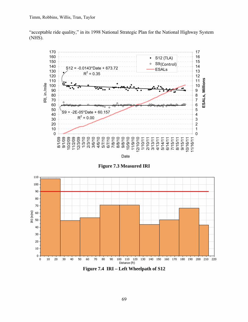
Timm, Robbins, Willis, Tran, Taylor
69
“acceptable ride quality,” in its 1998 National Strategic Plan for the National Highway System (NHS).
Figure 7.3 Measured IRI
Figure 7.4 IRI – Left Wheelpath of S12
S12 = -0.0143*Date + 673.72
R2 = 0.35
S9 = -2E-05*Date + 60.157
R2 = 0.00
0102030405060708090
100110120130140150160170
8/1
/09
9/1
/09
10/2
/09
11/2
/09
12/3
/09
1/3
/10
2/3
/10
3/6
/10
4/6
/10
5/7
/10
6/7
/10
7/8
/10
8/8
/10
9/8
/10
10/9
/10
11/9
/10
12/1
0/10
1/10
/11
2/10
/11
3/13
/11
4/13
/11
5/14
/11
6/14
/11
7/15
/11
8/15
/11
9/15
/11
10/1
6/11
11/1
6/11
Date
IRI,
in./m
ile
01234567891011121314151617
ES
AL
s, M
illio
ns
S12
S9
ESALs
(TLA)
(Control)
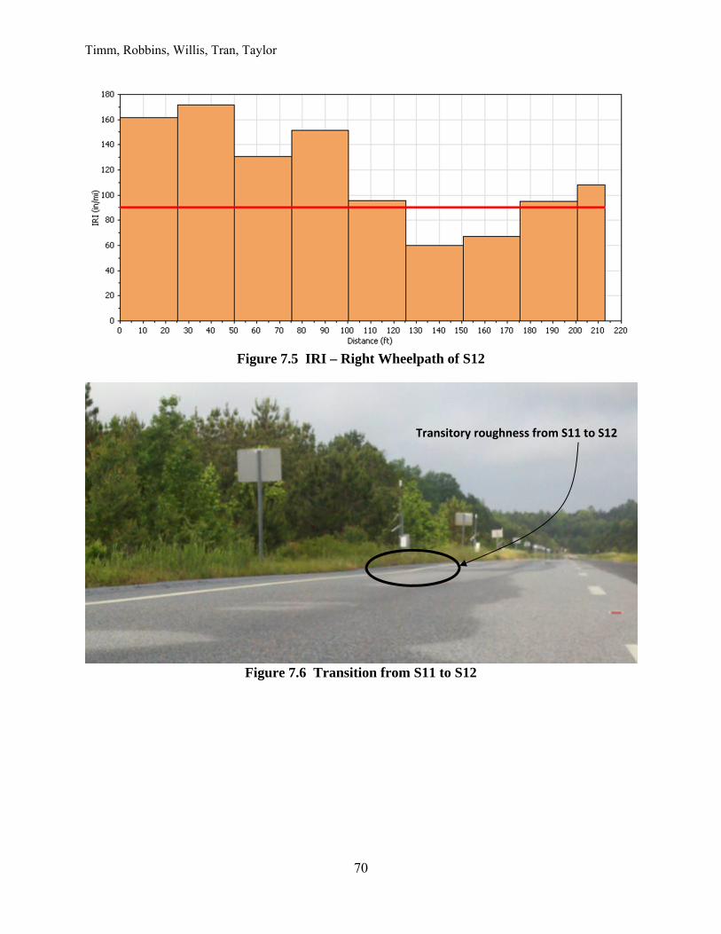
Timm, Robbins, Willis, Tran, Taylor
70
Figure 7.5 IRI – Right Wheelpath of S12
Figure 7.6 Transition from S11 to S12
Transitory roughness from S11 to S12
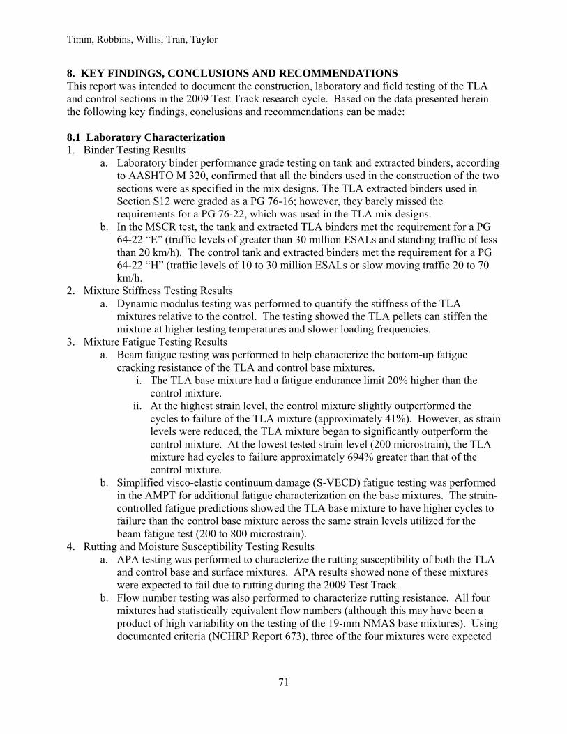
Timm, Robbins, Willis, Tran, Taylor
71
8. KEY FINDINGS, CONCLUSIONS AND RECOMMENDATIONS This report was intended to document the construction, laboratory and field testing of the TLA and control sections in the 2009 Test Track research cycle. Based on the data presented herein the following key findings, conclusions and recommendations can be made: 8.1 Laboratory Characterization 1. Binder Testing Results
a. Laboratory binder performance grade testing on tank and extracted binders, according to AASHTO M 320, confirmed that all the binders used in the construction of the two sections were as specified in the mix designs. The TLA extracted binders used in Section S12 were graded as a PG 76-16; however, they barely missed the requirements for a PG 76-22, which was used in the TLA mix designs.
b. In the MSCR test, the tank and extracted TLA binders met the requirement for a PG 64-22 “E” (traffic levels of greater than 30 million ESALs and standing traffic of less than 20 km/h). The control tank and extracted binders met the requirement for a PG 64-22 “H” (traffic levels of 10 to 30 million ESALs or slow moving traffic 20 to 70 km/h.
2. Mixture Stiffness Testing Results a. Dynamic modulus testing was performed to quantify the stiffness of the TLA
mixtures relative to the control. The testing showed the TLA pellets can stiffen the mixture at higher testing temperatures and slower loading frequencies.
3. Mixture Fatigue Testing Results a. Beam fatigue testing was performed to help characterize the bottom-up fatigue
cracking resistance of the TLA and control base mixtures. i. The TLA base mixture had a fatigue endurance limit 20% higher than the
control mixture. ii. At the highest strain level, the control mixture slightly outperformed the
cycles to failure of the TLA mixture (approximately 41%). However, as strain levels were reduced, the TLA mixture began to significantly outperform the control mixture. At the lowest tested strain level (200 microstrain), the TLA mixture had cycles to failure approximately 694% greater than that of the control mixture.
b. Simplified visco-elastic continuum damage (S-VECD) fatigue testing was performed in the AMPT for additional fatigue characterization on the base mixtures. The strain-controlled fatigue predictions showed the TLA base mixture to have higher cycles to failure than the control base mixture across the same strain levels utilized for the beam fatigue test (200 to 800 microstrain).
4. Rutting and Moisture Susceptibility Testing Results a. APA testing was performed to characterize the rutting susceptibility of both the TLA
and control base and surface mixtures. APA results showed none of these mixtures were expected to fail due to rutting during the 2009 Test Track.
b. Flow number testing was also performed to characterize rutting resistance. All four mixtures had statistically equivalent flow numbers (although this may have been a product of high variability on the testing of the 19-mm NMAS base mixtures). Using documented criteria (NCHRP Report 673), three of the four mixtures were expected
Timm, Robbins, Willis, Tran, Taylor
72
to have a traffic life of 3 to 10 million ESAL while the remaining mixture (TLA Base mixture) was expected to have a traffic life of 10 to 30 million ESAL.
i. Given that none of these mixtures experienced terminal rutting during the 2009 research cycle, it can be said that the NCHRP criteria were conservative with respect to these mixtures.
c. The Hamburg Wheel-Tracking test was used to characterize the rutting and moisture susceptibility of these mixtures. Based on the Hamburg results, neither rutting nor moisture susceptibility were anticipated to be an issue for these mixes during the 2009 research cycle.
d. The TSR results showed that none of the mixtures were anticipated to be susceptible to moisture damage.
5. Top-Down Cracking Susceptibility Testing a. The addition of the TLA pellets lowered the Energy Ratio (test for top-down cracking
resistance) of the surface mixture by a factor of three. However, the Energy Ratio of both mixtures still satisfied the minimum documented requirements to resist top-down cracking. At the conclusion of the 2009 test cycle, no top-down cracking had been observed in either section S12 or S9.
6. Thermal Cracking Susceptibility Testing a. The addition of the TLA pellets improved the thermal cracking resistance of both the
control and base mixtures according to the results from the IDT creep compliance and strength testing.
8.2 Construction 1. Both sections met or exceeded the compaction requirements during construction. The TLA
section, however, had lower in-place air voids overall which contributed to higher backcalculated moduli and lower measured pavement responses.
2. The program MultiCool was used to simulate the cooling of each AC lift placed during construction. The program predicted cooling rates adequately for each material and may be used to predict cooling of TLA-modified materials.
8.3 Structural Response Characterization 1. Backcalculated base and subgrade moduli were very similar between both test sections
indicating a uniform foundation below the AC layers. 2. The backcalculated AC modulus in both sections responded similarly to changes in
temperature. However, it was found that the TLA section had 20-24% higher modulus across the temperature spectrum. Statistical t-testing confirmed the differences in the normalized moduli were significant at three reference temperatures (50, 68 and 110°F). Since these differences were not evident in the laboratory dynamic modulus testing that utilized specimens compacted to the same density, the difference was attributed to lower in-place air voids.
3. Very little change was noted in backcalculated AC modulus versus time which indicated no significant aging effects nor damage to either section.
4. The four primary measured pavement responses (longitudinal strain, transverse strain, base pressure, subgrade pressure) all exhibited a strong correlation to mid-depth pavement temperature within each section.
Timm, Robbins, Willis, Tran, Taylor
73
5. Longitudinal strain measurements in the TLA section exhibited the greatest degree of variability. However, the variability was attributed to gauge functionality rather than pavement performance issues.
6. For each pavement response, differences between the TLA section and Control section became more pronounced at higher temperatures (110°F) while they tended to converge, and become indistinguishable, at lower temperatures (50°F).
7. Normalized longitudinal strain was 10% lower in the TLA section versus the control section at 110°F. At 50 and 68°F, the differences were not statistically significant. Despite similar strain levels at 68°F, when combined with the laboratory-derived fatigue transfer function, three times greater fatigue life for the TLA section was predicted.
8. Normalized transverse strain was 8% lower, and statistically significant, in the TLA section at 110°F. At 68°F, a statistical difference was noted but of such small magnitude (7 ) to be practically insignificant. At 50°F, no statistical differences were detected.
9. The base pressure measurements were remarkably consistent which lead to easily-detected statistical differences between sections. However, only at the highest temperature (110°F) was the difference in normalized pressure deemed practical with the TLA section 25% lower than the control. Normalized pressure at the lower temperatures (50 and 68°F) differed by less than 1.5 psi. Similar observations were made with the subgrade pressure measurements. At 110°F, the TLA section was 16% lower while less than 1 psi separated the sections at lower temperatures.
10. Lower measured vertical pressures in the TLA section, especially at high temperatures, stemmed from higher moduli resulting from higher in-place compacted density.
11. Pavement responses corrected to 68°F and plotted over time showed no indication of distress for either section. It is recommended to leave the sections in place for further monitoring in the 2012 research cycle.
8.4 Field Performance 1. After 10.14 million ESAL, neither section has experienced any cracking. 2. Slightly higher rut depths were measured with the ARAN van over time in the control section
relative to the TLA section. However, statistical testing using the final wireline measurements indicated no statistical differences between sections. Therefore, equivalent rutting performance was achieved between the sections.
3. Ride quality measurements, expressed as IRI, indicated that neither section became rougher over time and traffic. The control section maintained a nearly constant level of roughness. The TLA section actually decreased in roughness, by approximately 10 in./mile, over the two-year period. The TLA section had significantly higher roughness than the control section at the start of the experiment, but was attributed to construction issues rather than a material-related problem.
Timm, Robbins, Willis, Tran, Taylor
74
REFERENCES
1. Advanced Asphalt Technologies, LLC. NCHRP Report 673: A Manual for Designs of Hot Mix Asphalt with Commentary. Washington, DC: NCHRP, 2011.
2. Allen, D.L. and R.C. Graves. Variability in Measurement of In-Situ Material Properties. Proceedings, Fourth International Conference on the Bearing Capacity of Roads and Airfields, Vol. 2, 1994, pp. 989-1005.
3. Bennert, T. The Evaluation of Trinidad Lake Asphalt (TLA) in Hot Mix Asphalt: Phase 1 – Evaluation of Asphalt Binder PG Grades When Blended with TLA Pellets. Draft Final Report (Unpublished), Rutgers Asphalt/Pavement Laboratory, Piscataway, NJ.
4. Biel, T., B. Sharp, and R. Lindsey. Trinidad Lake Asphalt (TLA) Two Experimental Applications on I-80 from Echo to Canyon Rock. Final Report, Experimental Feature X(02)18, Utah Department of Transportation, 2006.
5. Bonaquist, R. Mix Design Practices for Warm Mix Asphalt. NCHRP Report 691, Washington, DC, National Cooperative Highway Research Program, 2011.
6. Buttlar W. G., R. Roque, and B. Reid. Automated Procedure for Generation of Creep Compliance Master Curve for Asphalt Mixtures. Transportation Research Record No. 1630, Washington, D.C., 1998, pp. 28-36.
7. Chadbourn, B.A., D.E. Newcomb, V.R. Voller, R.A. De Sombre, J.A. Luoma and D.H. Timm. An Asphalt Paving Tool for Adverse Conditions. Report MN/RC-1998-18, Minnesota Department of Transportation, 1998.
8. Daniel, J., and Y.R. Kim. Development of a Simplified Fatigue Test and Analysis Procedure Using a Viscoelastic, Continuum Damage Model. Journal of the Association of Asphalt Paving Technologists, Vol. 71, 2002, pp. 619-650.
9. Hiltunen, D. R., and R. Roque. A Mechanics-Based Prediction Model for Thermal Cracking of Asphaltic Concrete Pavements. Journal of the Association of Asphalt Paving Technologists, Vol. 63, 1994, pp. 81-117.
10. Hou, T., B.S. Underwood, and Y.R. Kim. Fatigue Performance Prediction of North Carolina Mixtures Using the Simplified Viscoelastic Continuum Damage Model. Journal of Association of Asphalt Paving Technologists, Vol. 79, 2010, pp. 35-80
11. Jones, G.M., M.I. Darter, and G. Littlefield. Thermal Expansion-Contraction of Asphaltic Concrete. Journal of the Association of Asphalt Paving Technologists, Vol. 37, 1968, pp. 56-97.
12. Kim, Y.R., H-J Lee, and D.N. Little. Fatigue Characterization of Asphalt Concrete Using Viscoelasticity and Continuum Damage Theory. Journal of Association of Asphalt Paving Technologists, Vol. 66, 1997, pp. 520-569.
13. Kim, J., R. Roque, and B. Birgisson. Integration of Thermal Fracture in the HMA Fracture Model. Journal of the Association of Asphalt Paving Technologists, Vol. 77, 2008, pp. 631-662.
14. LaForce, R. I-70 Glenwood Canyon Overlay with Trinidad Lake Asphalt/Steel Slag Hot Mix Asphalt. Report CDOT-DTD-R-2005-13, Colorado Department of Transportation, September, 2006.
15. Noureldin, A.S. Influence of Stress Levels and Seasonal Variations on In Situ Pavement Layer Properties. Transportation Research Record No. 1448, Washington, D.C., 1994, pp. 16-24.
Timm, Robbins, Willis, Tran, Taylor
75
16. Pelland, R., J. Gould, and R. Mallick. Selecting a Rut Resistant Hot Mix Asphalt for Boston-Logan International Airport. Airfield Pavements: Challenges and New Technologies, Airfield Pavements Specialty Conference, 2003, ASCE, 2003.
17. Priest, A.L. and D.H. Timm. Methodology and Calibration of Fatigue Transfer Functions for Mechanistic-Empirical Flexible Pavement Design. Report No. 06-03, National Center for Asphalt Technology, Auburn University, 2006.
18. Prowell, B.D., E.R. Brown, R.M. Anderson, J. Sias-Daniel, H. Von Quintus, S. Shen, S.H. Carpenter, S. Bhattacharjee and S. Maghsoodloo. Validating the Fatigue Endurance Limit for Hot Mix Asphalt. NCHRP Report 646, Transportation Research Board, Washington, D.C., 2010.
19. Roque, R., B. Birgisson, C. Drakos and B. Dietrich. Development and Field Evaluation of Energy-Based Criteria for Top-down Cracking Performance of Hot Mix Asphalt. Journal of the Association of Asphalt Paving Technologists, Vol. 73, 2004, pp. 229-260.
20. Roque, R., W.G. Buttlar, B.E. Ruth, M. Tia, S.W. Dickison and B. Reid. Evaluation of SHRP Indirect Tension Tester to Mitigate Cracking in Asphalt Concrete Pavements and Overlays. Final Report, University of Florida, Gainesville, Florida, 1997.
21. Russell, M., J. Uhlmeyer, K. Anderson, and J. Weston. Evaluation of Trinidad Lake Asphalt Overlay. Report WA-RD 710.1, Washington State Department of Transportation, September 2008.
22. Sebaaly, P., G. Bazi, and Y. Vivekanathan. Evaluation of New Pavement Technologies in Nevada. Report No. 13AX-1, Nevada Department of Transportation, 2003.
23. Soules, T.F., R.F. Busbey, S.M. Rekhson, A. Markovsky, and M. A. Burke. Finite-Element Calculation of Stresses in Glass Parts Undergoing Viscous Relaxation. Journal of the American Ceramic Society, 70 (2), 1987, pp. 90-95.
24. Taylor, A.J. and D.H. Timm. Mechanistic Characterization of Resilient Moduli for Unbound Pavement Layer Materials. Report No. 09-06, National Center for Asphalt Technology, Auburn University, 2009.
25. Timm, D.H. Design, Construction, and Instrumentation of the 2006 Test Track Structural Study. Report No. 09-01, National Center for Asphalt Technology, Auburn University, 2009.
26. Timm, D.H., D.E. Newcomb and B. Birgisson. Mechanistic-Empirical Flexible Pavement Thickness Design: The Minnesota Method. Staff Paper, MN/RC-P99-10, Minnesota Department of Transportation, St. Paul, MN, 1999.
27. Timm, D.H., G.A. Sholar, J. Kim, and J.R. Willis. Forensic Investigation and Validation of Energy Ratio Concept. Transportation Research Record No. 2127, Washington, D.C., 2009, pp. 43-51.
28. Timm, D.H. and A.L. Priest. Wheel Wander at the NCAT Test Track. Report No. 05-02, National Center for Asphalt Technology, Auburn University, 2005.
29. Timm, D.H. and A.L. Priest. Material Properties of the 2003 NCAT Test Track Structural Study. Report No. 06-01, National Center for Asphalt Technology, Auburn University, 2006.
30. Timm, D.H. and A.L. Priest. Flexible Pavement Fatigue Cracking and Measured Strain Response at the NCAT Test Track. Proceedings of the 87th Annual Transportation Research Board, Washington, D.C., 2008.
31. Timm, D.H., A.L. Priest and T.V. McEwen. Design and Instrumentation of the Structural Pavement Experiment at the NCAT Test Track. Report No. 04-01, National Center for Asphalt Technology, Auburn University, 2004.
Timm, Robbins, Willis, Tran, Taylor
76
32. Timm, D. H., V. R. Voller, E. Lee and J. Harvey. Calcool: A multi-layer Asphalt Pavement Cooling Tool for Temperature Prediction During Construction. The International Journal of Pavement Engineering, Vol. 2, 2001, pp. 169-185.
33. Underwood, B.S., Y.R. Kim and M. Guddati. Characterization and Performance Prediction of ALF Mixtures Using a Viscoelastoplastic Continuum Damage Model. Journal of Association of Asphalt Paving Technologists, Vol. 75, 2006, pp. 577-636.
34. Vargas-Nordcbeck, A. and D.H. Timm. Validation of Cooling Curves Prediction Model for Non-Conventional Asphalt Concrete Mixtures. Transportation Research Record No. 2228, Washington, D.C., 2011, pp. 111-119.
35. Widyatmoko, I., R. Elliot, and J. Reed. Development of Heavy-Duty Mastic Asphalt Bridge Surfacing, Incorporating Trinidad Lake Asphalt and Polymer Modified Binders. Journal of Road Materials and Pavement Design, Vol. 6, No. 4, 2005, pp. 469-483.
36. Willis, J.R. and D.H. Timm. Field-Based Strain Thresholds for Flexible Perpetual Pavement Design. Report No. 09-09, National Center for Asphalt Technology, Auburn University, 2009.
37. Witczak, M. Specification Criteria for Simple Performance Tests for Rutting. NCHRP Report 580, TRB, Washington, D.C., 2007.

Timm, Robbins, Willis, Tran, Taylor
77
APPENDIX A – MIX DESIGN AND AS BUILT AC PROPERTIES
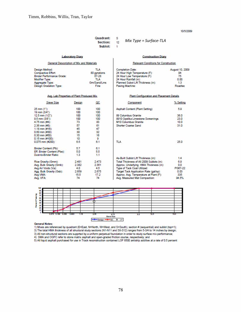
Timm, Robbins, Willis, Tran, Taylor
78
Mix Type = Surface‐TLA
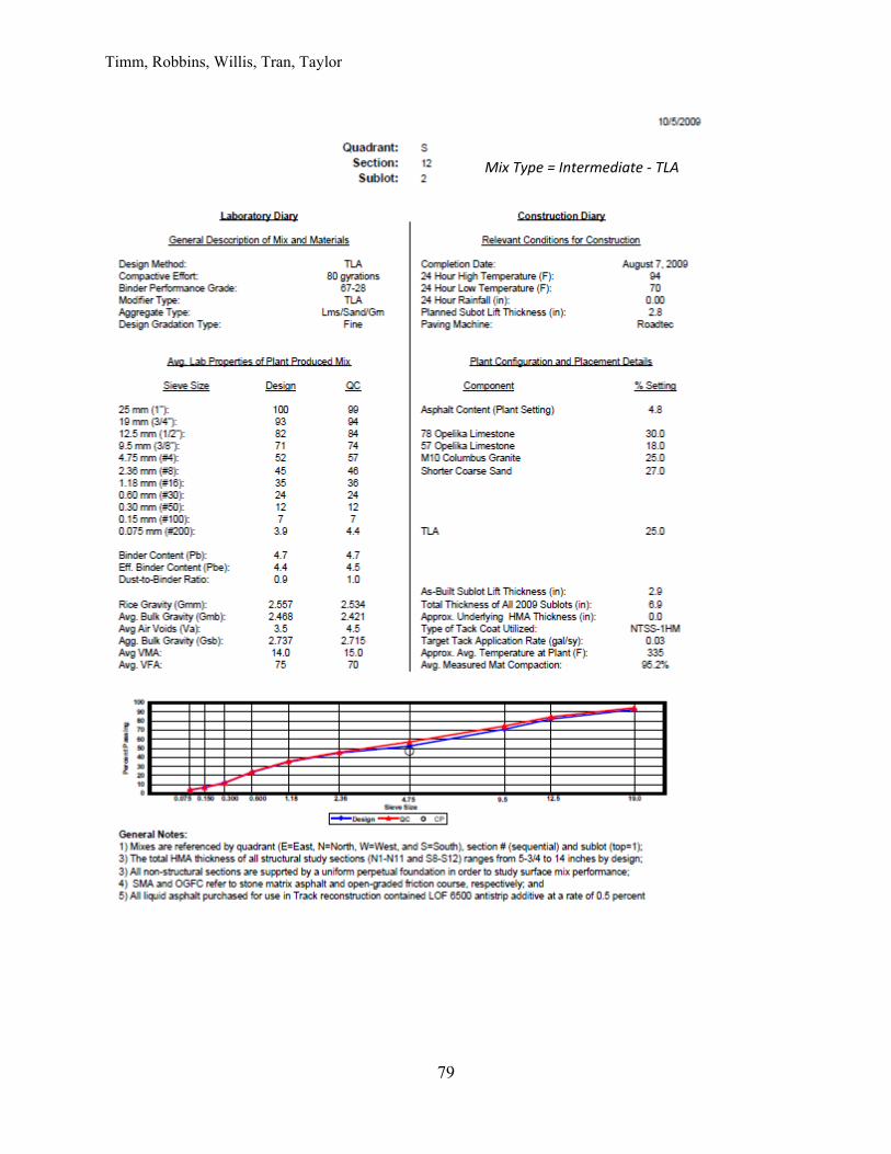
Timm, Robbins, Willis, Tran, Taylor
79
Mix Type = Intermediate ‐ TLA
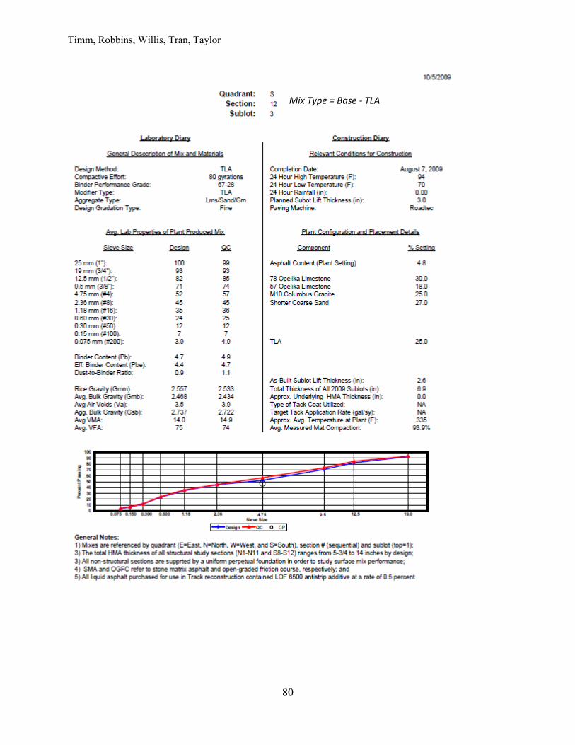
Timm, Robbins, Willis, Tran, Taylor
80
Mix Type = Base ‐ TLA
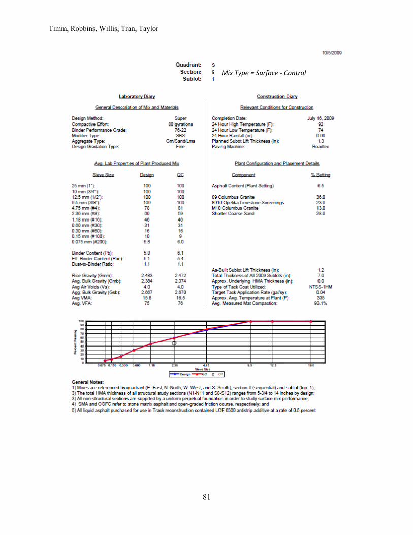
Timm, Robbins, Willis, Tran, Taylor
81
Mix Type = Surface ‐ Control
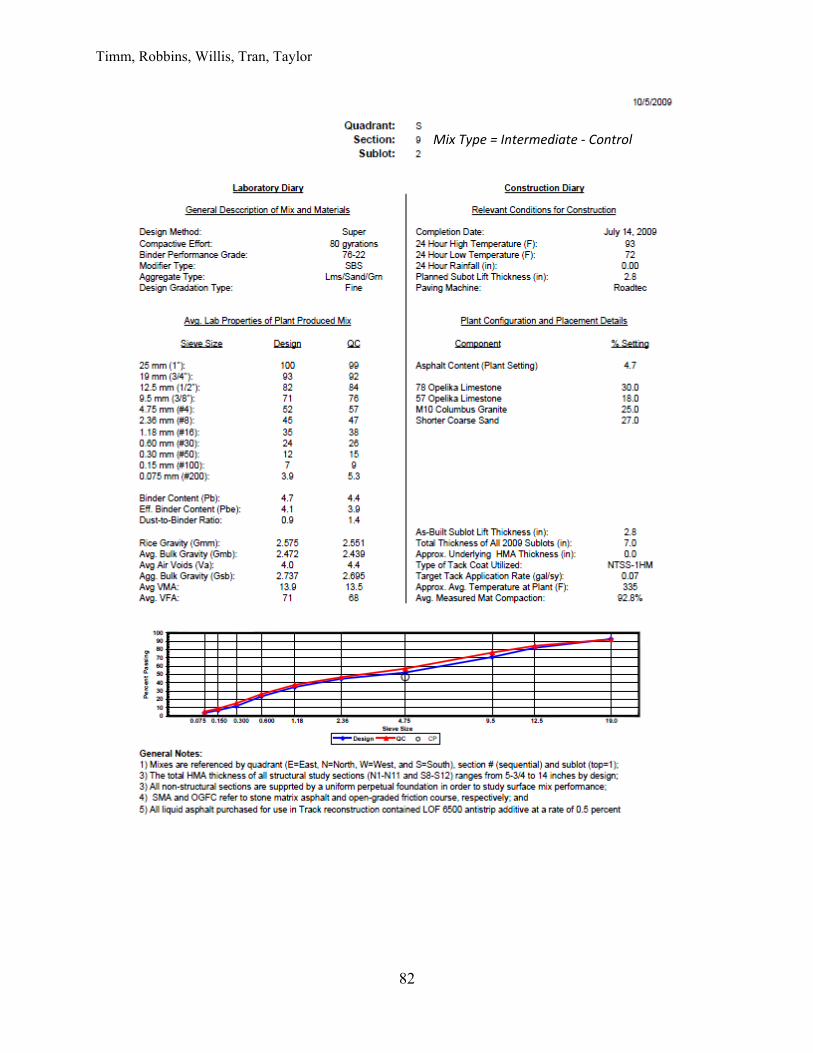
Timm, Robbins, Willis, Tran, Taylor
82
Mix Type = Intermediate ‐ Control
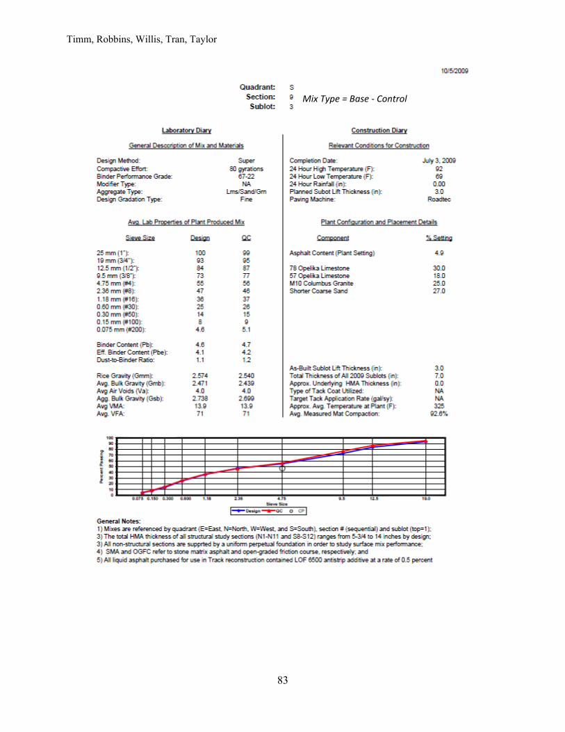
Timm, Robbins, Willis, Tran, Taylor
83
Mix Type = Base ‐ Control

Timm, Robbins, Willis, Tran, Taylor
84
APPENDIX B – SURVEYED PAVEMENT DEPTHS
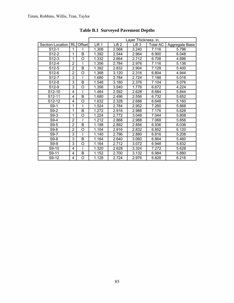
Timm, Robbins, Willis, Tran, Taylor
85
Table B.1 Surveyed Pavement Depths
Section-Location RL Offset Lift 1 Lift 2 Lift 3 Total AC Aggregate BaseS12-1 1 I 1.308 2.568 3.240 7.116 5.796S12-2 1 B 1.392 2.544 2.964 6.900 6.048S12-3 1 O 1.332 2.664 2.712 6.708 4.896S12-4 2 I 1.356 2.784 2.976 7.116 5.136S12-5 2 B 1.392 2.832 2.904 7.128 5.400S12-6 2 O 1.368 3.120 2.316 6.804 4.944S12-7 3 I 1.680 2.784 2.724 7.188 5.016S12-8 3 B 1.548 3.180 2.376 7.104 5.076S12-9 3 O 1.356 3.540 1.776 6.672 4.224
S12-10 4 I 1.464 2.592 2.628 6.684 5.844S12-11 4 B 1.680 2.496 2.556 6.732 5.652S12-12 4 O 1.632 2.328 2.688 6.648 5.160
S9-1 1 I 1.524 2.784 2.952 7.260 5.868S9-2 1 B 1.272 2.916 2.988 7.176 5.628S9-3 1 O 1.224 2.772 3.048 7.044 5.808S9-4 2 I 1.212 2.868 2.988 7.068 5.856S9-5 2 B 1.188 2.892 2.856 6.936 6.036S9-6 2 O 1.104 2.916 2.832 6.852 6.120S9-7 3 I 1.140 2.796 2.880 6.816 5.208S9-8 3 B 1.164 2.640 3.060 6.864 5.460S9-9 3 O 1.164 2.712 3.072 6.948 5.832
S9-10 4 I 1.320 2.628 3.324 7.272 5.628S9-11 4 B 1.152 2.700 3.132 6.984 5.880S9-12 4 O 1.128 2.724 2.976 6.828 6.216
Layer Thickness, in.

Timm, Robbins, Willis, Tran, Taylor
86
APPENDIX C – BINDER GRADING
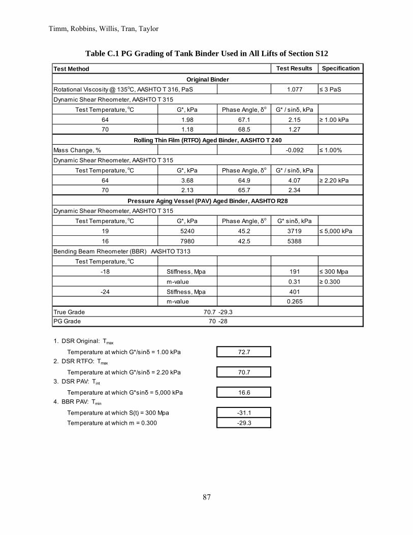
Timm, Robbins, Willis, Tran, Taylor
87
Table C.1 PG Grading of Tank Binder Used in All Lifts of Section S12
Test Results Specification
1.077 ≤ 3 PaS
Test Temperature, oC G*, kPa Phase Angle, δo G* / sinδ, kPa
64 1.98 67.1 2.15 ≥ 1.00 kPa
70 1.18 68.5 1.27
Mass Change, % -0.092 ≤ 1.00%
Test Temperature, oC G*, kPa Phase Angle, δo G* / sinδ, kPa
64 3.68 64.9 4.07 ≥ 2.20 kPa
70 2.13 65.7 2.34
Test Temperature, oC G*, kPa Phase Angle, δo G* sinδ, kPa
19 5240 45.2 3719 ≤ 5,000 kPa
16 7980 42.5 5388
Test Temperature, oC
-18 Stiffness, Mpa 191 ≤ 300 Mpa
m-value 0.31 ≥ 0.300
-24 Stiffness, Mpa 401
m-value 0.265
True Grade 70.7 -29.3
PG Grade 70 -28
1. DSR Original: Tmax
Temperature at which G*/sinδ = 1.00 kPa 72.7
2. DSR RTFO: Tmax
Temperature at which G*/sinδ = 2.20 kPa 70.7
3. DSR PAV: Tint
Temperature at which G*sinδ = 5,000 kPa 16.6
4. BBR PAV: Tmin
Temperature at which S(t) = 300 Mpa -31.1
Temperature at which m = 0.300 -29.3
Dynamic Shear Rheometer, AASHTO T 315
Bending Beam Rheometer (BBR) AASHTO T313
Dynamic Shear Rheometer, AASHTO T 315
Dynamic Shear Rheometer, AASHTO T 315
Rotational Viscosity @ 135oC, AASHTO T 316, PaS
Original Binder
Rolling Thin Film (RTFO) Aged Binder, AASHTO T 240
Pressure Aging Vessel (PAV) Aged Binder, AASHTO R28
Test Method

Timm, Robbins, Willis, Tran, Taylor
88
Table C.2 PG Grading of Binder Extracted from Base and Binder Mixtures of Section S12 (Replicate 1)
Test Method Test Results Specification
2.472 ≤ 3 PaS
Test Temperature, oC G*, kPa Phase Angle, δo G* / sinδ, kPa
82 2.17 73.3 2.26 ≥ 2.20 kPa88 1.2 75.7 1.24
Test Temperature, oC G*, kPa Phase Angle, δo G* sinδ, kPa
28 6990 43.1 4775 ≤ 5,000 kPa25 10300 40.5 6684
Test Temperature, oC-6 Stiffness, Mpa 103 ≤ 300 Mpa
m-value 0.335 ≥ 0.300-12 Stiffness, Mpa 204
m-value 0.296
True Grade 82.3 -21.4PG Grade 82 -16
1. DSR RTFO: Tmax
82.3
2. DSR PAV: Tint
27.6
3. BBR PAV: Tmin
-27.7
-21.4
Temperature at which G*/sinδ = 2.20 kPa
Temperature at which G*sinδ = 5,000 kPa
Tempearautre at which S(t) = 300 Mpa
Temperature at which m = 0.300
Rolling Thin Film Oven (RTFO) Aged Binder, AASHTO T 240
Pressure Aging Vessel (PAV) Aged Binder, AASHTO R28
Dynamic Shear Rheometer, AASHTO T 315
Dynamic Shear Rheometer, AASHTO T 315
Bending Beam Rheometer (BBR), AASHTO T313
Rotational Viscosity @ 135oC, AASHTO T 316, PaS
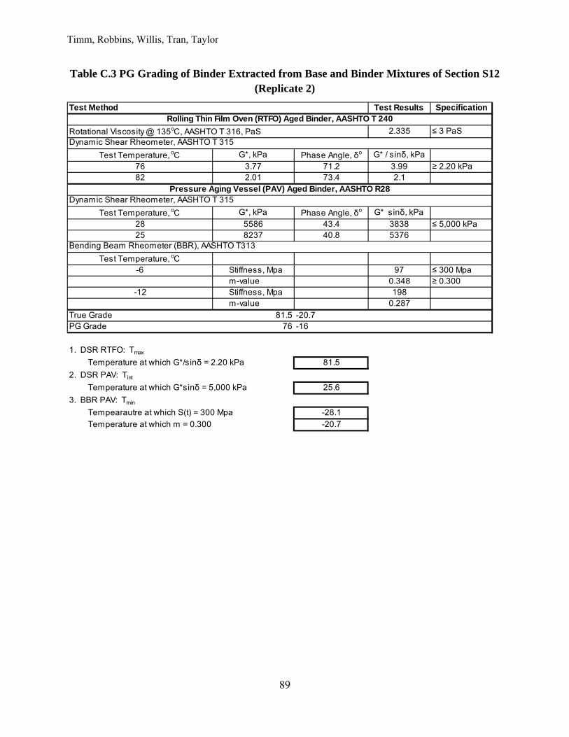
Timm, Robbins, Willis, Tran, Taylor
89
Table C.3 PG Grading of Binder Extracted from Base and Binder Mixtures of Section S12 (Replicate 2)
Test Results Specification
2.335 ≤ 3 PaS
Test Temperature, oC G*, kPa Phase Angle, δo G* / sinδ, kPa
76 3.77 71.2 3.99 ≥ 2.20 kPa82 2.01 73.4 2.1
Test Temperature, oC G*, kPa Phase Angle, δo G* sinδ, kPa
28 5586 43.4 3838 ≤ 5,000 kPa25 8237 40.8 5376
Test Temperature, oC-6 Stiffness, Mpa 97 ≤ 300 Mpa
m-value 0.348 ≥ 0.300-12 Stiffness, Mpa 198
m-value 0.287
True Grade 81.5 -20.7PG Grade 76 -16
1. DSR RTFO: Tmax
81.5
2. DSR PAV: Tint
25.6
3. BBR PAV: Tmin
-28.1
-20.7
Test Method
Temperature at which G*/sinδ = 2.20 kPa
Temperature at which G*sinδ = 5,000 kPa
Tempearautre at which S(t) = 300 Mpa
Temperature at which m = 0.300
Rolling Thin Film Oven (RTFO) Aged Binder, AASHTO T 240
Pressure Aging Vessel (PAV) Aged Binder, AASHTO R28
Rotational Viscosity @ 135oC, AASHTO T 316, PaSDynamic Shear Rheometer, AASHTO T 315
Dynamic Shear Rheometer, AASHTO T 315
Bending Beam Rheometer (BBR), AASHTO T313

Timm, Robbins, Willis, Tran, Taylor
90
Table C.4 PG Grading of Binder Extracted from Surface Mixture of Section S12 (Replicate 1)
Test Results Specification
2.4 ≤ 3 PaS
Test Temperature, oC G*, kPa Phase Angle, δo G* / sinδ, kPa
76 3.88 70.8 4.11 ≥ 2.20 kPa82 2.06 72.8 2.16
Test Temperature, oC G*, kPa Phase Angle, δo G* sinδ, kPa
31 5603 46.2 4043 ≤ 5,000 kPa28 8162 43.9 5662
Test Temperature, oC-6 Stiffness, Mpa 108 ≤ 300 Mpa
m-value 0.33 ≥ 0.300-12 Stiffness, Mpa 209
m-value 0.288
True Grade 81.8 -20.3PG Grade 76 -16
1. DSR RTFO: Tmax
81.8
2. DSR PAV: Tint
29.1
3. BBR PAV: Tmin
-27.4
-20.3
Temperature at which G*/sinδ = 2.20 kPa
Temperature at which G*sinδ = 5,000 kPa
Tempearautre at which S(t) = 300 Mpa
Temperature at which m = 0.300
Test MethodRolling Thin Film Oven (RTFO) Aged Binder, AASHTO T 240
Pressure Aging Vessel (PAV) Aged Binder, AASHTO R28
Dynamic Shear Rheometer, AASHTO T 315
Dynamic Shear Rheometer, AASHTO T 315
Bending Beam Rheometer (BBR), AASHTO T 313
Rotational Viscosity @ 135oC, AASHTO T 316, PaS

Timm, Robbins, Willis, Tran, Taylor
91
Table C.5 PG Grading of Binder Extracted from Surface Mixture of Section S12 (Replicate 2)
Test Results Specification
2.21 ≤ 3 PaS
Test Temperature, oC G*, kPa Phase Angle, δo G* / sinδ, kPa
76 3.33 71.8 3.51 ≥ 2.20 kPa82 1.81 73.7 1.89
Test Temperature, oC G*, kPa Phase Angle, δo G* sinδ, kPa
28 6092 43.9 4226 ≤ 5,000 kPa25 9022 41.3 5954
Test Temperature, oC-6 Stiffness, Mpa 107 ≤ 300 Mpa
m-value 0.343 ≥ 0.300-12 Stiffness, Mpa 216
m-value 0.292
True Grade 80.5 -21.1PG Grade 76 -16
1. DSR RTFO: Tmax
80.5
2. DSR PAV: Tint
26.5
3. BBR PAV: Tmin
-26.6
-21.1
Temperature at which G*/sinδ = 2.20 kPa
Temperature at which G*sinδ = 5,000 kPa
Tempearautre at which S(t) = 300 Mpa
Temperature at which m = 0.300
Test MethodRolling Thin Film Oven (RTFO) Aged Binder, AASHTO T 240
Pressure Aging Vessel (PAV) Aged Binder, AASHTO R28
Dynamic Shear Rheometer, AASHTO T 315
Dynamic Shear Rheometer, AASHTO T 315
Bending Beam Rheometer (BBR), AASHTO T313
Rotational Viscosity @ 135oC, AASHTO T 316, PaS

Timm, Robbins, Willis, Tran, Taylor
92
Table C.6 PG Grading of Tank Binder Used in Base Lift of Section S9
Test Method Test Results Specification
≤ 3 PaS
Dynamic Shear Rheometer AASHTO T 315
Test Temperature, oC G*, kPa Phase Angle δ, o G* / sinδ, kPa
64 1.91 84.9 1.91 ≥ 1.00 kPa
70 0.94 86.3 0.94
Mass Change, % ≤ 1.00%
Dynamic Shear Rheometer AASHTO T 315
Test Temperature, oC G*, kPa Phase Angle δ, o G* / sinδ, kPa
70 2.40 82.4 2.42 ≥ 2.20 kPa
76 1.186 84.5 1.19
Dynamic Shear Rheometer AASHTO T 315
Test Temperature, oC G*, kPa Phase Angle δ, o G* sinδ, kPa
22 6245 41.9 4169 ≤ 5,000 kPa
19 9212 39.3 5837
Bending Beam Rheometer (BBR) AASHTO T313
Test Temperature, oC
-12 Stiffness, Mpa 141 ≤ 300 Mpa
m-value 0.333 ≥ 0.300
-18 Stiffness, Mpa 313
m-value 0.283
True Grade 69.5 -26.0
PG Grade 64 - 22
1. DSR Original: Tmax
69.5
2. DSR RTFO: Tmax
70.8
3. DSR PAV: Tint
20.4
4. BBR PAV: Tmin
-27.5
-26.0
Original Binder
Rolling Thin Film (RTFO) Aged Binder, AASHTO T 240
Pressure Aging Vessel (PAV) Aged Binder, AASHTO R28
Rotational Viscosity @ 135oC, AASHTO T 316, PaS
Temperature at which G*/sinδ = 1.00 kPa
Temperature at which G*/sinδ = 2.20 kPa
Temperature at which G*sinδ = 5,000 kPa
Temperature at which S(t) = 300 Mpa
Temperature at which m = 0.300
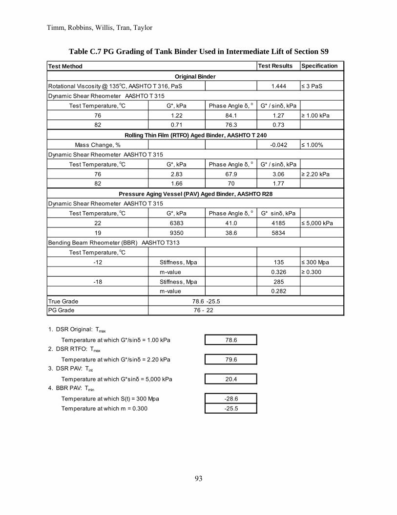
Timm, Robbins, Willis, Tran, Taylor
93
Table C.7 PG Grading of Tank Binder Used in Intermediate Lift of Section S9
Test Results Specification
1.444 ≤ 3 PaS
Test Temperature, oC G*, kPa Phase Angle δ, o G* / sinδ, kPa
76 1.22 84.1 1.27 ≥ 1.00 kPa
82 0.71 76.3 0.73
Mass Change, % -0.042 ≤ 1.00%
Test Temperature, oC G*, kPa Phase Angle δ, o G* / sinδ, kPa
76 2.83 67.9 3.06 ≥ 2.20 kPa
82 1.66 70 1.77
Test Temperature, oC G*, kPa Phase Angle δ, o G* sinδ, kPa
22 6383 41.0 4185 ≤ 5,000 kPa
19 9350 38.6 5834
Test Temperature, oC
-12 Stiffness, Mpa 135 ≤ 300 Mpa
m-value 0.326 ≥ 0.300
-18 Stiffness, Mpa 285
m-value 0.282
True Grade 78.6 -25.5
PG Grade 76 - 22
1. DSR Original: Tmax
78.6
2. DSR RTFO: Tmax
79.6
3. DSR PAV: Tint
20.4
4. BBR PAV: Tmin
-28.6
-25.5
Dynamic Shear Rheometer AASHTO T 315
Bending Beam Rheometer (BBR) AASHTO T313
Dynamic Shear Rheometer AASHTO T 315
Dynamic Shear Rheometer AASHTO T 315
Original Binder
Rolling Thin Film (RTFO) Aged Binder, AASHTO T 240
Pressure Aging Vessel (PAV) Aged Binder, AASHTO R28
Rotational Viscosity @ 135oC, AASHTO T 316, PaS
Test Method
Temperature at which G*/sinδ = 1.00 kPa
Temperature at which G*/sinδ = 2.20 kPa
Temperature at which G*sinδ = 5,000 kPa
Temperature at which S(t) = 300 Mpa
Temperature at which m = 0.300
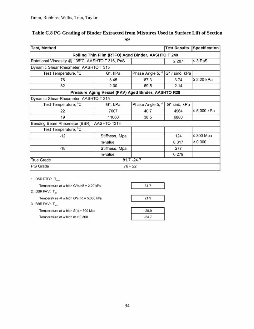
Timm, Robbins, Willis, Tran, Taylor
94
Table C.8 PG Grading of Binder Extracted from Mixtures Used in Surface Lift of Section S9
Test, Method Test Results Specification
Rotational Viscosity @ 135oC, AASHTO T 316, PaS 2.287 ≤ 3 PaS
Test Temperature, oC G*, kPa Phase Angle δ, o G* / sinδ, kPa
76 3.45 67.3 3.74 ≥ 2.20 kPa
82 2.00 69.5 2.14
Test Temperature, oC G*, kPa Phase Angle δ, o G* sinδ, kPa
22 7607 40.7 4964 ≤ 5,000 kPa
19 11060 38.5 6880
Test Temperature, oC
-12 Stiffness, Mpa 124 ≤ 300 Mpa
m-value 0.317 ≥ 0.300
-18 Stiffness, Mpa 277
m-value 0.279True Grade 81.7 -24.7
PG Grade 76 - 22
1. DSR RTFO: Tmax
Temperature at w hich G*/sinδ = 2.20 kPa 81.7
2. DSR PAV: Tint
Temperature at w hich G*sinδ = 5,000 kPa 21.9
3. BBR PAV: Tmin
Temperature at w hich S(t) = 300 Mpa -28.9
Temperature at w hich m = 0.300 -24.7
Dynamic Shear Rheometer AASHTO T 315
Dynamic Shear Rheometer AASHTO T 315
Bending Beam Rheometer (BBR) AASHTO T313
Rolling Thin Film (RTFO) Aged Binder, AASHTO T 240
Pressure Aging Vessel (PAV) Aged Binder, AASHTO R28

Timm, Robbins, Willis, Tran, Taylor
95
APPENDIX D - MASTER CURVE DATA

Timm, Robbins, Willis, Tran, Taylor
96
Table D.1 MEPDG Input values for Dynamic Modulus Testing (Unconfined) Section‐Lift ID Temp
(deg C) Temp (deg F)
Frequency (Hz)
Shift Factor
Reduced Frequency
E*, (ksi)
E*, (Mpa)
CONTROL‐SURFACE ‐10.0 14 25 4.035 2.71E+05 2516.5 17356.1
CONTROL‐SURFACE ‐10.0 14 10 4.035 1.09E+05 2418.3 16679.0
CONTROL‐SURFACE ‐10.0 14 5 4.035 5.43E+04 2334.7 16102.4
CONTROL‐SURFACE ‐10.0 14 1 4.035 1.09E+04 2108.1 14539.8
CONTROL‐SURFACE ‐10.0 14 0.5 4.035 5.43E+03 1996.7 13771.1
CONTROL‐SURFACE ‐10.0 14 0.1 4.035 1.09E+03 1709.2 11788.0
CONTROL‐SURFACE 4.4 40 25 1.984 2.41E+03 1856.1 12801.8
CONTROL‐SURFACE 4.4 40 10 1.984 9.63E+02 1686.5 11631.5
CONTROL‐SURFACE 4.4 40 5 1.984 4.81E+02 1551.9 10703.6
CONTROL‐SURFACE 4.4 40 1 1.984 9.63E+01 1229.4 8479.3
CONTROL‐SURFACE 4.4 40 0.5 1.984 4.81E+01 1091.3 7526.5
CONTROL‐SURFACE 4.4 40 0.1 1.984 9.63E+00 789.0 5442.0
CONTROL‐SURFACE 21.1 70 25 ‐0.134 1.84E+01 906.1 6249.6
CONTROL‐SURFACE 21.1 70 10 ‐0.134 7.35E+00 742.3 5119.7
CONTROL‐SURFACE 21.1 70 5 ‐0.134 3.68E+00 629.1 4338.8
CONTROL‐SURFACE 21.1 70 1 ‐0.134 7.35E‐01 409.1 2821.8
CONTROL‐SURFACE 21.1 70 0.5 ‐0.134 3.68E‐01 334.0 2303.5
CONTROL‐SURFACE 21.1 70 0.1 ‐0.134 7.35E‐02 202.3 1395.4
CONTROL‐SURFACE 37.8 100 25 ‐2.024 2.37E‐01 292.2 2015.5
CONTROL‐SURFACE 37.8 100 10 ‐2.024 9.46E‐02 219.3 1512.8
CONTROL‐SURFACE 37.8 100 5 ‐2.024 4.73E‐02 175.5 1210.5
CONTROL‐SURFACE 37.8 100 1 ‐2.024 9.46E‐03 104.0 717.2
CONTROL‐SURFACE 37.8 100 0.5 ‐2.024 4.73E‐03 83.3 574.3
CONTROL‐SURFACE 37.8 100 0.1 ‐2.024 9.46E‐04 50.9 350.9
CONTROL‐SURFACE 54.4 130 25 ‐3.722 4.74E‐03 83.3 574.7
CONTROL‐SURFACE 54.4 130 10 ‐3.722 1.90E‐03 62.6 431.9
CONTROL‐SURFACE 54.4 130 5 ‐3.722 9.48E‐04 50.9 351.1
CONTROL‐SURFACE 54.4 130 1 ‐3.722 1.90E‐04 32.7 225.6
CONTROL‐SURFACE 54.4 130 0.5 ‐3.722 9.48E‐05 27.6 190.1
CONTROL‐SURFACE 54.4 130 0.1 ‐3.722 1.90E‐05 19.4 134.0
TLA – SURFACE ‐10.0 14 25 3.740 1.37E+05 2715.5 18728.8
TLA – SURFACE ‐10.0 14 10 3.740 5.49E+04 2632.2 18154.4
TLA – SURFACE ‐10.0 14 5 3.740 2.75E+04 2558.6 17646.7
TLA – SURFACE ‐10.0 14 1 3.740 5.49E+03 2347.7 16192.0
TLA – SURFACE ‐10.0 14 0.5 3.740 2.75E+03 2238.3 15437.4
TLA – SURFACE ‐10.0 14 0.1 3.740 5.49E+02 1940.5 13383.5
TLA – SURFACE 4.4 40 25 1.838 1.72E+03 2158.2 14885.2
TLA – SURFACE 4.4 40 10 1.838 6.89E+02 1986.0 13697.6
TLA – SURFACE 4.4 40 5 1.838 3.44E+02 1843.6 12715.3
TLA – SURFACE 4.4 40 1 1.838 6.89E+01 1482.0 10221.4
TLA – SURFACE 4.4 40 0.5 1.838 3.44E+01 1318.9 9096.7
TLA – SURFACE 4.4 40 0.1 1.838 6.89E+00 947.4 6534.3
TLA – SURFACE 21.1 70 25 ‐0.124 1.88E+01 1176.5 8114.2
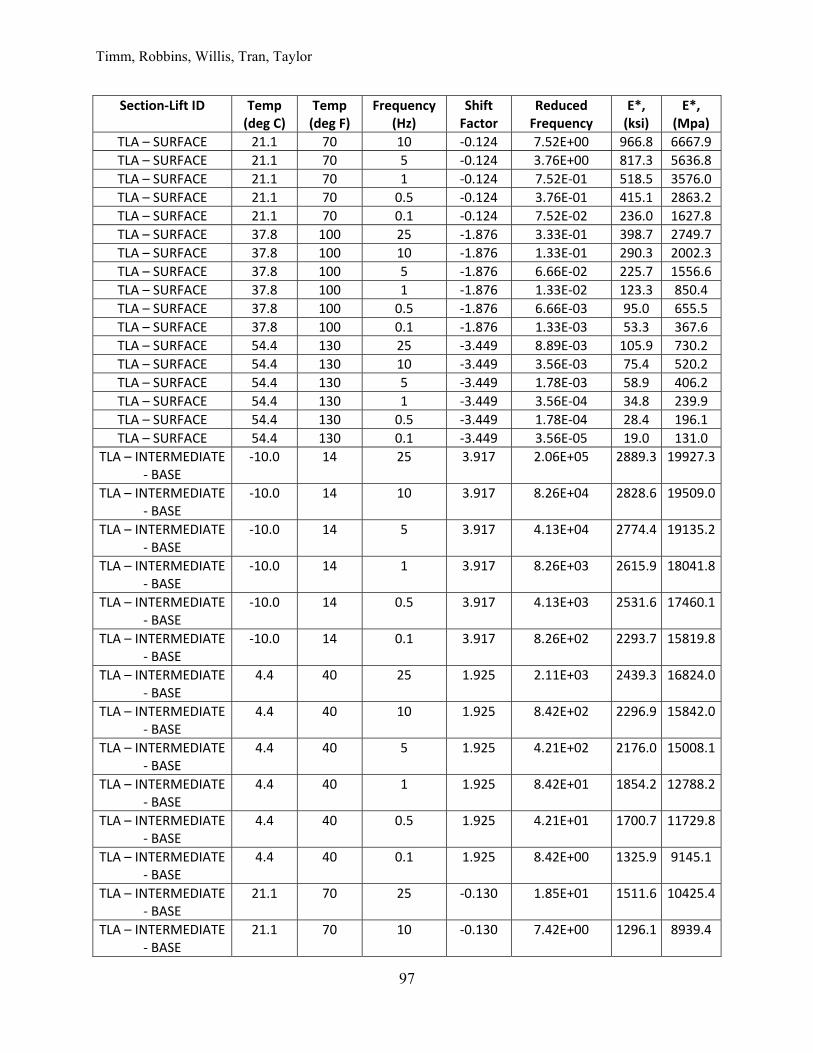
Timm, Robbins, Willis, Tran, Taylor
97
Section‐Lift ID Temp (deg C)
Temp (deg F)
Frequency (Hz)
Shift Factor
Reduced Frequency
E*, (ksi)
E*, (Mpa)
TLA – SURFACE 21.1 70 10 ‐0.124 7.52E+00 966.8 6667.9
TLA – SURFACE 21.1 70 5 ‐0.124 3.76E+00 817.3 5636.8
TLA – SURFACE 21.1 70 1 ‐0.124 7.52E‐01 518.5 3576.0
TLA – SURFACE 21.1 70 0.5 ‐0.124 3.76E‐01 415.1 2863.2
TLA – SURFACE 21.1 70 0.1 ‐0.124 7.52E‐02 236.0 1627.8
TLA – SURFACE 37.8 100 25 ‐1.876 3.33E‐01 398.7 2749.7
TLA – SURFACE 37.8 100 10 ‐1.876 1.33E‐01 290.3 2002.3
TLA – SURFACE 37.8 100 5 ‐1.876 6.66E‐02 225.7 1556.6
TLA – SURFACE 37.8 100 1 ‐1.876 1.33E‐02 123.3 850.4
TLA – SURFACE 37.8 100 0.5 ‐1.876 6.66E‐03 95.0 655.5
TLA – SURFACE 37.8 100 0.1 ‐1.876 1.33E‐03 53.3 367.6
TLA – SURFACE 54.4 130 25 ‐3.449 8.89E‐03 105.9 730.2
TLA – SURFACE 54.4 130 10 ‐3.449 3.56E‐03 75.4 520.2
TLA – SURFACE 54.4 130 5 ‐3.449 1.78E‐03 58.9 406.2
TLA – SURFACE 54.4 130 1 ‐3.449 3.56E‐04 34.8 239.9
TLA – SURFACE 54.4 130 0.5 ‐3.449 1.78E‐04 28.4 196.1
TLA – SURFACE 54.4 130 0.1 ‐3.449 3.56E‐05 19.0 131.0
TLA – INTERMEDIATE ‐ BASE
‐10.0 14 25 3.917 2.06E+05 2889.3 19927.3
TLA – INTERMEDIATE ‐ BASE
‐10.0 14 10 3.917 8.26E+04 2828.6 19509.0
TLA – INTERMEDIATE ‐ BASE
‐10.0 14 5 3.917 4.13E+04 2774.4 19135.2
TLA – INTERMEDIATE ‐ BASE
‐10.0 14 1 3.917 8.26E+03 2615.9 18041.8
TLA – INTERMEDIATE ‐ BASE
‐10.0 14 0.5 3.917 4.13E+03 2531.6 17460.1
TLA – INTERMEDIATE ‐ BASE
‐10.0 14 0.1 3.917 8.26E+02 2293.7 15819.8
TLA – INTERMEDIATE ‐ BASE
4.4 40 25 1.925 2.11E+03 2439.3 16824.0
TLA – INTERMEDIATE ‐ BASE
4.4 40 10 1.925 8.42E+02 2296.9 15842.0
TLA – INTERMEDIATE ‐ BASE
4.4 40 5 1.925 4.21E+02 2176.0 15008.1
TLA – INTERMEDIATE ‐ BASE
4.4 40 1 1.925 8.42E+01 1854.2 12788.2
TLA – INTERMEDIATE ‐ BASE
4.4 40 0.5 1.925 4.21E+01 1700.7 11729.8
TLA – INTERMEDIATE ‐ BASE
4.4 40 0.1 1.925 8.42E+00 1325.9 9145.1
TLA – INTERMEDIATE ‐ BASE
21.1 70 25 ‐0.130 1.85E+01 1511.6 10425.4
TLA – INTERMEDIATE ‐ BASE
21.1 70 10 ‐0.130 7.42E+00 1296.1 8939.4
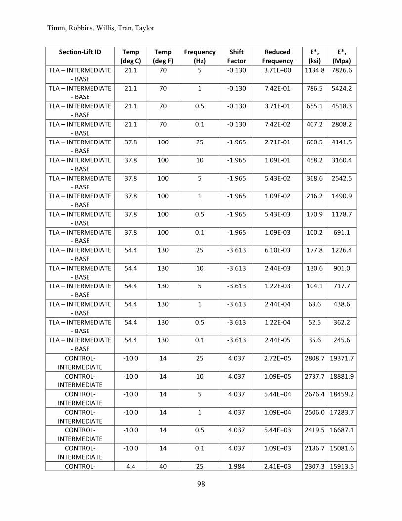
Timm, Robbins, Willis, Tran, Taylor
98
Section‐Lift ID Temp (deg C)
Temp (deg F)
Frequency (Hz)
Shift Factor
Reduced Frequency
E*, (ksi)
E*, (Mpa)
TLA – INTERMEDIATE ‐ BASE
21.1 70 5 ‐0.130 3.71E+00 1134.8 7826.6
TLA – INTERMEDIATE ‐ BASE
21.1 70 1 ‐0.130 7.42E‐01 786.5 5424.2
TLA – INTERMEDIATE ‐ BASE
21.1 70 0.5 ‐0.130 3.71E‐01 655.1 4518.3
TLA – INTERMEDIATE ‐ BASE
21.1 70 0.1 ‐0.130 7.42E‐02 407.2 2808.2
TLA – INTERMEDIATE ‐ BASE
37.8 100 25 ‐1.965 2.71E‐01 600.5 4141.5
TLA – INTERMEDIATE ‐ BASE
37.8 100 10 ‐1.965 1.09E‐01 458.2 3160.4
TLA – INTERMEDIATE ‐ BASE
37.8 100 5 ‐1.965 5.43E‐02 368.6 2542.5
TLA – INTERMEDIATE ‐ BASE
37.8 100 1 ‐1.965 1.09E‐02 216.2 1490.9
TLA – INTERMEDIATE ‐ BASE
37.8 100 0.5 ‐1.965 5.43E‐03 170.9 1178.7
TLA – INTERMEDIATE ‐ BASE
37.8 100 0.1 ‐1.965 1.09E‐03 100.2 691.1
TLA – INTERMEDIATE ‐ BASE
54.4 130 25 ‐3.613 6.10E‐03 177.8 1226.4
TLA – INTERMEDIATE ‐ BASE
54.4 130 10 ‐3.613 2.44E‐03 130.6 901.0
TLA – INTERMEDIATE ‐ BASE
54.4 130 5 ‐3.613 1.22E‐03 104.1 717.7
TLA – INTERMEDIATE ‐ BASE
54.4 130 1 ‐3.613 2.44E‐04 63.6 438.6
TLA – INTERMEDIATE ‐ BASE
54.4 130 0.5 ‐3.613 1.22E‐04 52.5 362.2
TLA – INTERMEDIATE ‐ BASE
54.4 130 0.1 ‐3.613 2.44E‐05 35.6 245.6
CONTROL‐INTERMEDIATE
‐10.0 14 25 4.037 2.72E+05 2808.7 19371.7
CONTROL‐INTERMEDIATE
‐10.0 14 10 4.037 1.09E+05 2737.7 18881.9
CONTROL‐INTERMEDIATE
‐10.0 14 5 4.037 5.44E+04 2676.4 18459.2
CONTROL‐INTERMEDIATE
‐10.0 14 1 4.037 1.09E+04 2506.0 17283.7
CONTROL‐INTERMEDIATE
‐10.0 14 0.5 4.037 5.44E+03 2419.5 16687.1
CONTROL‐INTERMEDIATE
‐10.0 14 0.1 4.037 1.09E+03 2186.7 15081.6
CONTROL‐ 4.4 40 25 1.984 2.41E+03 2307.3 15913.5

Timm, Robbins, Willis, Tran, Taylor
99
Section‐Lift ID Temp (deg C)
Temp (deg F)
Frequency (Hz)
Shift Factor
Reduced Frequency
E*, (ksi)
E*, (Mpa)
INTERMEDIATE
CONTROL‐INTERMEDIATE
4.4 40 10 1.984 9.64E+02 2167.4 14948.4
CONTROL‐INTERMEDIATE
4.4 40 5 1.984 4.82E+02 2052.2 14154.0
CONTROL‐INTERMEDIATE
4.4 40 1 1.984 9.64E+01 1757.5 12121.2
CONTROL‐INTERMEDIATE
4.4 40 0.5 1.984 4.82E+01 1621.4 11182.5
CONTROL‐INTERMEDIATE
4.4 40 0.1 1.984 9.64E+00 1295.7 8936.7
CONTROL‐INTERMEDIATE
21.1 70 25 ‐0.134 1.84E+01 1426.8 9840.4
CONTROL‐INTERMEDIATE
21.1 70 10 ‐0.134 7.35E+00 1240.8 8557.6
CONTROL‐INTERMEDIATE
21.1 70 5 ‐0.134 3.68E+00 1102.4 7603.4
CONTROL‐INTERMEDIATE
21.1 70 1 ‐0.134 7.35E‐01 802.0 5531.5
CONTROL‐INTERMEDIATE
21.1 70 0.5 ‐0.134 3.68E‐01 686.2 4733.1
CONTROL‐INTERMEDIATE
21.1 70 0.1 ‐0.134 7.35E‐02 458.6 3163.1
CONTROL‐INTERMEDIATE
37.8 100 25 ‐2.025 2.36E‐01 617.7 4260.5
CONTROL‐INTERMEDIATE
37.8 100 10 ‐2.025 9.45E‐02 490.1 3380.2
CONTROL‐INTERMEDIATE
37.8 100 5 ‐2.025 4.72E‐02 406.9 2806.2
CONTROL‐INTERMEDIATE
37.8 100 1 ‐2.025 9.45E‐03 256.7 1770.3
CONTROL‐INTERMEDIATE
37.8 100 0.5 ‐2.025 4.72E‐03 208.7 1439.7
CONTROL‐INTERMEDIATE
37.8 100 0.1 ‐2.025 9.45E‐04 128.6 886.7
CONTROL‐INTERMEDIATE
54.4 130 25 ‐3.723 4.73E‐03 208.8 1440.1
CONTROL‐INTERMEDIATE
54.4 130 10 ‐3.723 1.89E‐03 158.4 1092.5
CONTROL‐INTERMEDIATE
54.4 130 5 ‐3.723 9.46E‐04 128.6 886.9
CONTROL‐INTERMEDIATE
54.4 130 1 ‐3.723 1.89E‐04 80.3 554.0
CONTROL‐INTERMEDIATE
54.4 130 0.5 ‐3.723 9.46E‐05 66.3 457.1
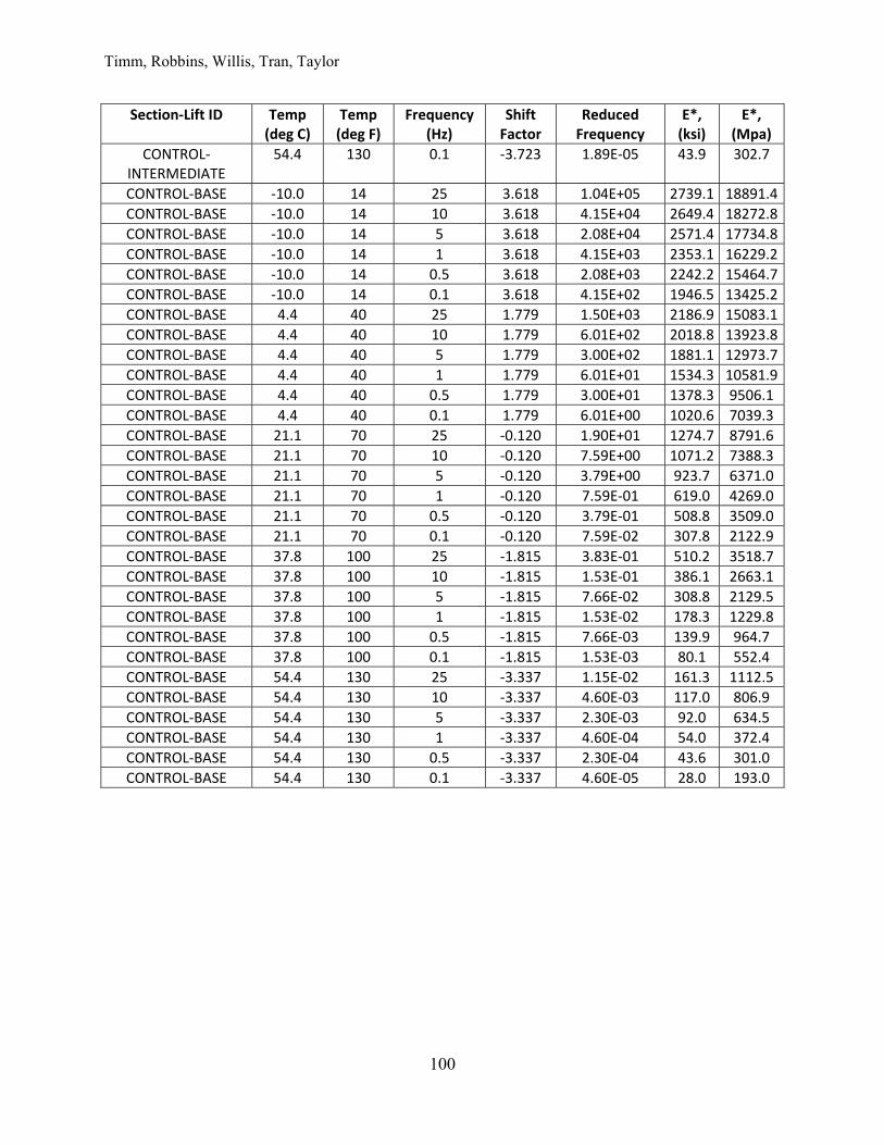
Timm, Robbins, Willis, Tran, Taylor
100
Section‐Lift ID Temp (deg C)
Temp (deg F)
Frequency (Hz)
Shift Factor
Reduced Frequency
E*, (ksi)
E*, (Mpa)
CONTROL‐INTERMEDIATE
54.4 130 0.1 ‐3.723 1.89E‐05 43.9 302.7
CONTROL‐BASE ‐10.0 14 25 3.618 1.04E+05 2739.1 18891.4
CONTROL‐BASE ‐10.0 14 10 3.618 4.15E+04 2649.4 18272.8
CONTROL‐BASE ‐10.0 14 5 3.618 2.08E+04 2571.4 17734.8
CONTROL‐BASE ‐10.0 14 1 3.618 4.15E+03 2353.1 16229.2
CONTROL‐BASE ‐10.0 14 0.5 3.618 2.08E+03 2242.2 15464.7
CONTROL‐BASE ‐10.0 14 0.1 3.618 4.15E+02 1946.5 13425.2
CONTROL‐BASE 4.4 40 25 1.779 1.50E+03 2186.9 15083.1
CONTROL‐BASE 4.4 40 10 1.779 6.01E+02 2018.8 13923.8
CONTROL‐BASE 4.4 40 5 1.779 3.00E+02 1881.1 12973.7
CONTROL‐BASE 4.4 40 1 1.779 6.01E+01 1534.3 10581.9
CONTROL‐BASE 4.4 40 0.5 1.779 3.00E+01 1378.3 9506.1
CONTROL‐BASE 4.4 40 0.1 1.779 6.01E+00 1020.6 7039.3
CONTROL‐BASE 21.1 70 25 ‐0.120 1.90E+01 1274.7 8791.6
CONTROL‐BASE 21.1 70 10 ‐0.120 7.59E+00 1071.2 7388.3
CONTROL‐BASE 21.1 70 5 ‐0.120 3.79E+00 923.7 6371.0
CONTROL‐BASE 21.1 70 1 ‐0.120 7.59E‐01 619.0 4269.0
CONTROL‐BASE 21.1 70 0.5 ‐0.120 3.79E‐01 508.8 3509.0
CONTROL‐BASE 21.1 70 0.1 ‐0.120 7.59E‐02 307.8 2122.9
CONTROL‐BASE 37.8 100 25 ‐1.815 3.83E‐01 510.2 3518.7
CONTROL‐BASE 37.8 100 10 ‐1.815 1.53E‐01 386.1 2663.1
CONTROL‐BASE 37.8 100 5 ‐1.815 7.66E‐02 308.8 2129.5
CONTROL‐BASE 37.8 100 1 ‐1.815 1.53E‐02 178.3 1229.8
CONTROL‐BASE 37.8 100 0.5 ‐1.815 7.66E‐03 139.9 964.7
CONTROL‐BASE 37.8 100 0.1 ‐1.815 1.53E‐03 80.1 552.4
CONTROL‐BASE 54.4 130 25 ‐3.337 1.15E‐02 161.3 1112.5
CONTROL‐BASE 54.4 130 10 ‐3.337 4.60E‐03 117.0 806.9
CONTROL‐BASE 54.4 130 5 ‐3.337 2.30E‐03 92.0 634.5
CONTROL‐BASE 54.4 130 1 ‐3.337 4.60E‐04 54.0 372.4
CONTROL‐BASE 54.4 130 0.5 ‐3.337 2.30E‐04 43.6 301.0
CONTROL‐BASE 54.4 130 0.1 ‐3.337 4.60E‐05 28.0 193.0
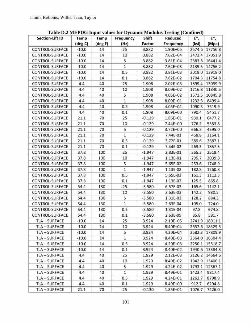
Timm, Robbins, Willis, Tran, Taylor
101
Table D.2 MEPDG Input values for Dynamic Modulus Testing (Confined) Section‐Lift ID Temp
(deg C) Temp (deg F)
Frequency (Hz)
Shift Factor
Reduced Frequency
E*, (ksi)
E*, (Mpa)
CONTROL‐SURFACE ‐10.0 14 25 3.882 1.90E+05 2574.6 17756.8
CONTROL‐SURFACE ‐10.0 14 10 3.882 7.62E+04 2472.4 17051.9
CONTROL‐SURFACE ‐10.0 14 5 3.882 3.81E+04 2383.8 16441.4
CONTROL‐SURFACE ‐10.0 14 1 3.882 7.62E+03 2139.5 14756.2
CONTROL‐SURFACE ‐10.0 14 0.5 3.882 3.81E+03 2018.0 13918.0
CONTROL‐SURFACE ‐10.0 14 0.1 3.882 7.62E+02 1704.3 11754.8
CONTROL‐SURFACE 4.4 40 25 1.908 2.02E+03 1899.4 13099.9
CONTROL‐SURFACE 4.4 40 10 1.908 8.09E+02 1716.8 11840.5
CONTROL‐SURFACE 4.4 40 5 1.908 4.05E+02 1572.5 10845.8
CONTROL‐SURFACE 4.4 40 1 1.908 8.09E+01 1232.3 8499.4
CONTROL‐SURFACE 4.4 40 0.5 1.908 4.05E+01 1090.3 7519.9
CONTROL‐SURFACE 4.4 40 0.1 1.908 8.09E+00 790.4 5451.7
CONTROL‐SURFACE 21.1 70 25 ‐0.129 1.86E+01 939.1 6477.2
CONTROL‐SURFACE 21.1 70 10 ‐0.129 7.44E+00 776.2 5353.8
CONTROL‐SURFACE 21.1 70 5 ‐0.129 3.72E+00 666.2 4595.0
CONTROL‐SURFACE 21.1 70 1 ‐0.129 7.44E‐01 458.8 3164.1
CONTROL‐SURFACE 21.1 70 0.5 ‐0.129 3.72E‐01 389.6 2687.1
CONTROL‐SURFACE 21.1 70 0.1 ‐0.129 7.44E‐02 269.3 1857.5
CONTROL‐SURFACE 37.8 100 25 ‐1.947 2.83E‐01 365.3 2519.4
CONTROL‐SURFACE 37.8 100 10 ‐1.947 1.13E‐01 295.7 2039.8
CONTROL‐SURFACE 37.8 100 5 ‐1.947 5.65E‐02 253.6 1748.9
CONTROL‐SURFACE 37.8 100 1 ‐1.947 1.13E‐02 182.8 1260.8
CONTROL‐SURFACE 37.8 100 0.5 ‐1.947 5.65E‐03 161.3 1112.3
CONTROL‐SURFACE 37.8 100 0.1 ‐1.947 1.13E‐03 125.5 865.8
CONTROL‐SURFACE 54.4 130 25 ‐3.580 6.57E‐03 165.6 1142.1
CONTROL‐SURFACE 54.4 130 10 ‐3.580 2.63E‐03 142.2 980.5
CONTROL‐SURFACE 54.4 130 5 ‐3.580 1.31E‐03 128.2 884.3
CONTROL‐SURFACE 54.4 130 1 ‐3.580 2.63E‐04 105.0 724.0
CONTROL‐SURFACE 54.4 130 0.5 ‐3.580 1.31E‐04 97.8 674.8
CONTROL‐SURFACE 54.4 130 0.1 ‐3.580 2.63E‐05 85.8 591.7
TLA – SURFACE ‐10.0 14 25 3.924 2.10E+05 2741.9 18911.1
TLA – SURFACE ‐10.0 14 10 3.924 8.40E+04 2657.6 18329.5
TLA – SURFACE ‐10.0 14 5 3.924 4.20E+04 2582.3 17809.9
TLA – SURFACE ‐10.0 14 1 3.924 8.40E+03 2364.0 16304.4
TLA – SURFACE ‐10.0 14 0.5 3.924 4.20E+03 2250.1 15518.7
TLA – SURFACE ‐10.0 14 0.1 3.924 8.40E+02 1940.6 13384.3
TLA – SURFACE 4.4 40 25 1.929 2.12E+03 2126.2 14664.6
TLA – SURFACE 4.4 40 10 1.929 8.49E+02 1942.9 13400.1
TLA – SURFACE 4.4 40 5 1.929 4.24E+02 1793.1 12367.1
TLA – SURFACE 4.4 40 1 1.929 8.49E+01 1423.4 9817.4
TLA – SURFACE 4.4 40 0.5 1.929 4.24E+01 1262.7 8708.9
TLA – SURFACE 4.4 40 0.1 1.929 8.49E+00 912.7 6294.8
TLA – SURFACE 21.1 70 25 ‐0.130 1.85E+01 1076.7 7426.0
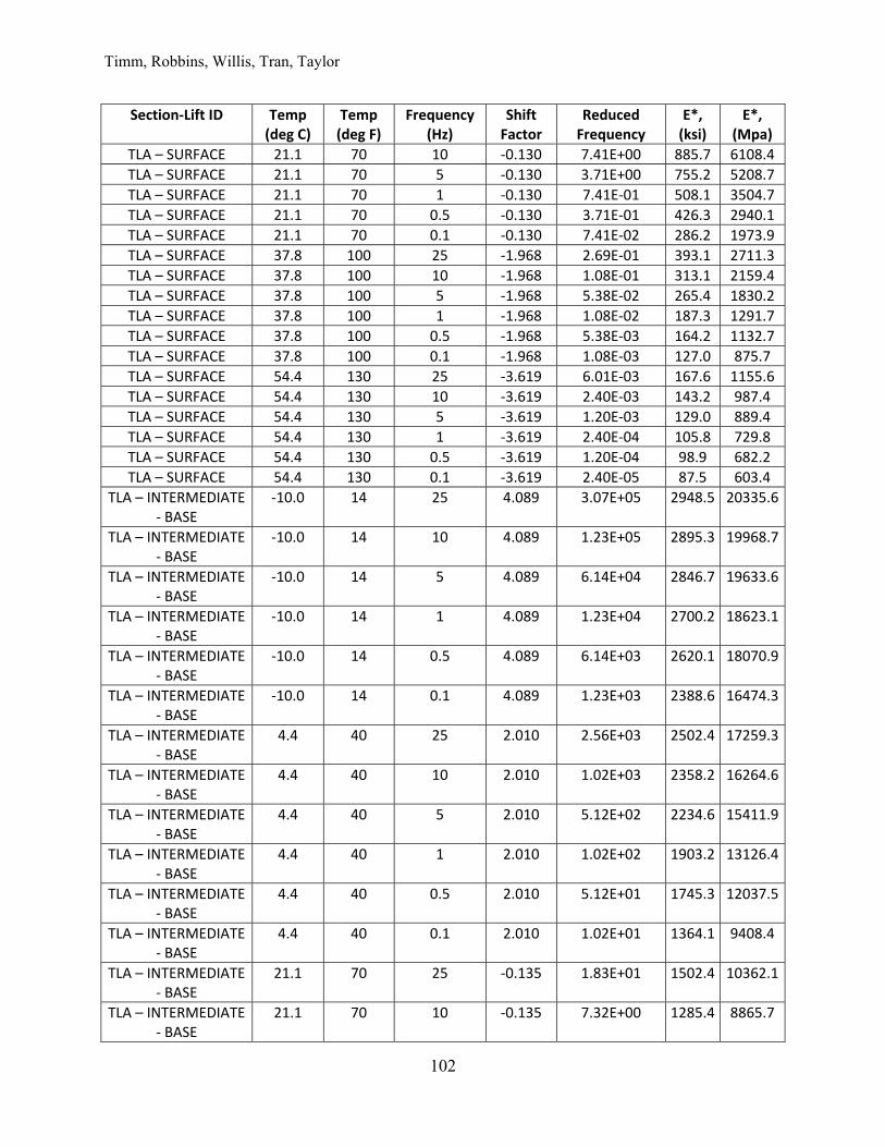
Timm, Robbins, Willis, Tran, Taylor
102
Section‐Lift ID Temp (deg C)
Temp (deg F)
Frequency (Hz)
Shift Factor
Reduced Frequency
E*, (ksi)
E*, (Mpa)
TLA – SURFACE 21.1 70 10 ‐0.130 7.41E+00 885.7 6108.4
TLA – SURFACE 21.1 70 5 ‐0.130 3.71E+00 755.2 5208.7
TLA – SURFACE 21.1 70 1 ‐0.130 7.41E‐01 508.1 3504.7
TLA – SURFACE 21.1 70 0.5 ‐0.130 3.71E‐01 426.3 2940.1
TLA – SURFACE 21.1 70 0.1 ‐0.130 7.41E‐02 286.2 1973.9
TLA – SURFACE 37.8 100 25 ‐1.968 2.69E‐01 393.1 2711.3
TLA – SURFACE 37.8 100 10 ‐1.968 1.08E‐01 313.1 2159.4
TLA – SURFACE 37.8 100 5 ‐1.968 5.38E‐02 265.4 1830.2
TLA – SURFACE 37.8 100 1 ‐1.968 1.08E‐02 187.3 1291.7
TLA – SURFACE 37.8 100 0.5 ‐1.968 5.38E‐03 164.2 1132.7
TLA – SURFACE 37.8 100 0.1 ‐1.968 1.08E‐03 127.0 875.7
TLA – SURFACE 54.4 130 25 ‐3.619 6.01E‐03 167.6 1155.6
TLA – SURFACE 54.4 130 10 ‐3.619 2.40E‐03 143.2 987.4
TLA – SURFACE 54.4 130 5 ‐3.619 1.20E‐03 129.0 889.4
TLA – SURFACE 54.4 130 1 ‐3.619 2.40E‐04 105.8 729.8
TLA – SURFACE 54.4 130 0.5 ‐3.619 1.20E‐04 98.9 682.2
TLA – SURFACE 54.4 130 0.1 ‐3.619 2.40E‐05 87.5 603.4
TLA – INTERMEDIATE ‐ BASE
‐10.0 14 25 4.089 3.07E+05 2948.5 20335.6
TLA – INTERMEDIATE ‐ BASE
‐10.0 14 10 4.089 1.23E+05 2895.3 19968.7
TLA – INTERMEDIATE ‐ BASE
‐10.0 14 5 4.089 6.14E+04 2846.7 19633.6
TLA – INTERMEDIATE ‐ BASE
‐10.0 14 1 4.089 1.23E+04 2700.2 18623.1
TLA – INTERMEDIATE ‐ BASE
‐10.0 14 0.5 4.089 6.14E+03 2620.1 18070.9
TLA – INTERMEDIATE ‐ BASE
‐10.0 14 0.1 4.089 1.23E+03 2388.6 16474.3
TLA – INTERMEDIATE ‐ BASE
4.4 40 25 2.010 2.56E+03 2502.4 17259.3
TLA – INTERMEDIATE ‐ BASE
4.4 40 10 2.010 1.02E+03 2358.2 16264.6
TLA – INTERMEDIATE ‐ BASE
4.4 40 5 2.010 5.12E+02 2234.6 15411.9
TLA – INTERMEDIATE ‐ BASE
4.4 40 1 2.010 1.02E+02 1903.2 13126.4
TLA – INTERMEDIATE ‐ BASE
4.4 40 0.5 2.010 5.12E+01 1745.3 12037.5
TLA – INTERMEDIATE ‐ BASE
4.4 40 0.1 2.010 1.02E+01 1364.1 9408.4
TLA – INTERMEDIATE ‐ BASE
21.1 70 25 ‐0.135 1.83E+01 1502.4 10362.1
TLA – INTERMEDIATE ‐ BASE
21.1 70 10 ‐0.135 7.32E+00 1285.4 8865.7
Timm, Robbins, Willis, Tran, Taylor
103
Section‐Lift ID Temp (deg C)
Temp (deg F)
Frequency (Hz)
Shift Factor
Reduced Frequency
E*, (ksi)
E*, (Mpa)
TLA – INTERMEDIATE ‐ BASE
21.1 70 5 ‐0.135 3.66E+00 1126.7 7771.2
TLA – INTERMEDIATE ‐ BASE
21.1 70 1 ‐0.135 7.32E‐01 797.0 5496.9
TLA – INTERMEDIATE ‐ BASE
21.1 70 0.5 ‐0.135 3.66E‐01 677.5 4672.8
TLA – INTERMEDIATE ‐ BASE
21.1 70 0.1 ‐0.135 7.32E‐02 458.5 3162.5
TLA – INTERMEDIATE ‐ BASE
37.8 100 25 ‐2.051 2.22E‐01 601.0 4145.1
TLA – INTERMEDIATE ‐ BASE
37.8 100 10 ‐2.051 8.90E‐02 480.8 3316.1
TLA – INTERMEDIATE ‐ BASE
37.8 100 5 ‐2.051 4.45E‐02 406.5 2803.8
TLA – INTERMEDIATE ‐ BASE
37.8 100 1 ‐2.051 8.90E‐03 280.8 1936.8
TLA – INTERMEDIATE ‐ BASE
37.8 100 0.5 ‐2.051 4.45E‐03 242.8 1674.8
TLA – INTERMEDIATE ‐ BASE
37.8 100 0.1 ‐2.051 8.90E‐04 180.9 1247.6
TLA – INTERMEDIATE ‐ BASE
54.4 130 25 ‐3.771 4.23E‐03 240.4 1658.1
TLA – INTERMEDIATE ‐ BASE
54.4 130 10 ‐3.771 1.69E‐03 201.9 1392.8
TLA – INTERMEDIATE ‐ BASE
54.4 130 5 ‐3.771 8.46E‐04 179.4 1237.6
TLA – INTERMEDIATE ‐ BASE
54.4 130 1 ‐3.771 1.69E‐04 142.9 985.3
TLA – INTERMEDIATE ‐ BASE
54.4 130 0.5 ‐3.771 8.46E‐05 132.0 910.2
TLA – INTERMEDIATE ‐ BASE
54.4 130 0.1 ‐3.771 1.69E‐05 114.1 786.8
CONTROL‐INTERMEDIATE
‐10.0 14 25 4.116 3.27E+05 2878.7 19854.1
CONTROL‐INTERMEDIATE
‐10.0 14 10 4.116 1.31E+05 2810.0 19380.7
CONTROL‐INTERMEDIATE
‐10.0 14 5 4.116 6.54E+04 2749.4 18962.7
CONTROL‐INTERMEDIATE
‐10.0 14 1 4.116 1.31E+04 2575.7 17764.9
CONTROL‐INTERMEDIATE
‐10.0 14 0.5 4.116 6.54E+03 2485.4 17141.9
CONTROL‐INTERMEDIATE
‐10.0 14 0.1 4.116 1.31E+03 2237.7 15433.4
CONTROL‐ 4.4 40 25 2.023 2.64E+03 2352.3 16223.6
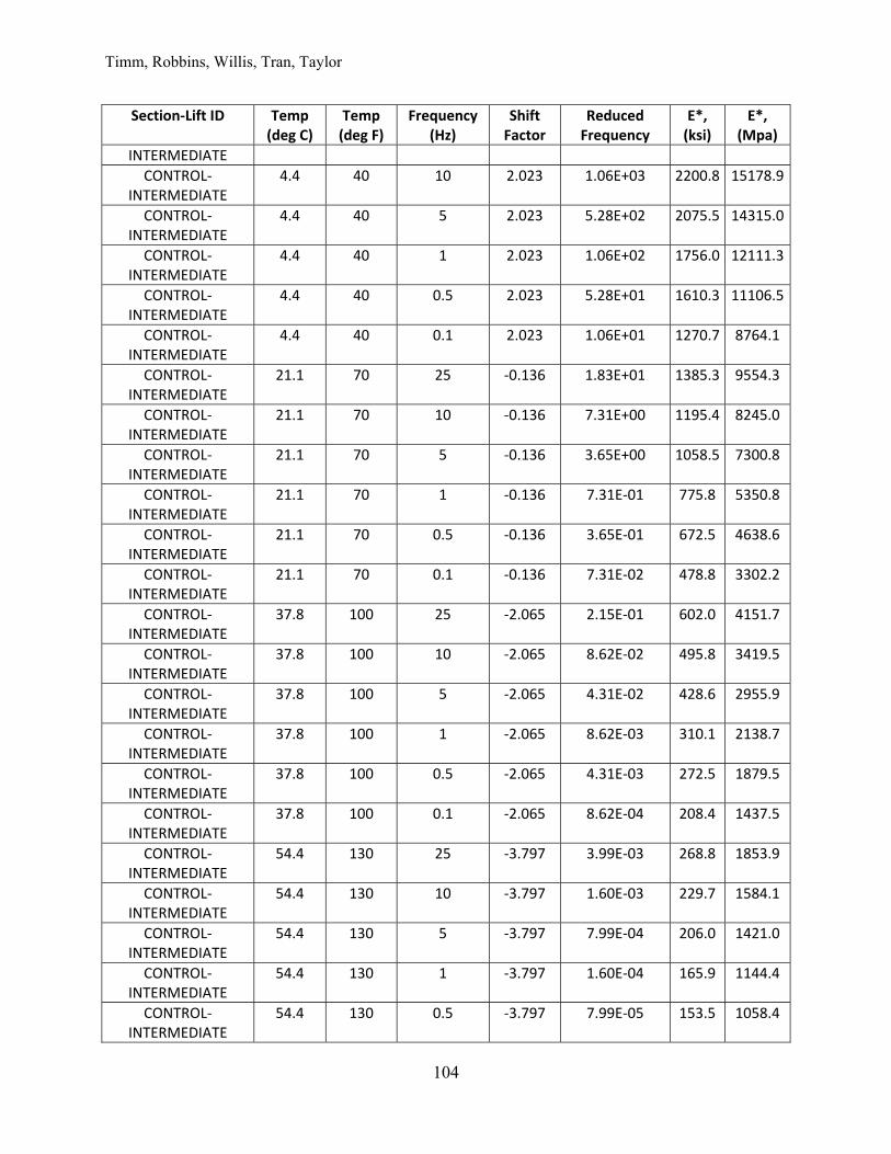
Timm, Robbins, Willis, Tran, Taylor
104
Section‐Lift ID Temp (deg C)
Temp (deg F)
Frequency (Hz)
Shift Factor
Reduced Frequency
E*, (ksi)
E*, (Mpa)
INTERMEDIATE
CONTROL‐INTERMEDIATE
4.4 40 10 2.023 1.06E+03 2200.8 15178.9
CONTROL‐INTERMEDIATE
4.4 40 5 2.023 5.28E+02 2075.5 14315.0
CONTROL‐INTERMEDIATE
4.4 40 1 2.023 1.06E+02 1756.0 12111.3
CONTROL‐INTERMEDIATE
4.4 40 0.5 2.023 5.28E+01 1610.3 11106.5
CONTROL‐INTERMEDIATE
4.4 40 0.1 2.023 1.06E+01 1270.7 8764.1
CONTROL‐INTERMEDIATE
21.1 70 25 ‐0.136 1.83E+01 1385.3 9554.3
CONTROL‐INTERMEDIATE
21.1 70 10 ‐0.136 7.31E+00 1195.4 8245.0
CONTROL‐INTERMEDIATE
21.1 70 5 ‐0.136 3.65E+00 1058.5 7300.8
CONTROL‐INTERMEDIATE
21.1 70 1 ‐0.136 7.31E‐01 775.8 5350.8
CONTROL‐INTERMEDIATE
21.1 70 0.5 ‐0.136 3.65E‐01 672.5 4638.6
CONTROL‐INTERMEDIATE
21.1 70 0.1 ‐0.136 7.31E‐02 478.8 3302.2
CONTROL‐INTERMEDIATE
37.8 100 25 ‐2.065 2.15E‐01 602.0 4151.7
CONTROL‐INTERMEDIATE
37.8 100 10 ‐2.065 8.62E‐02 495.8 3419.5
CONTROL‐INTERMEDIATE
37.8 100 5 ‐2.065 4.31E‐02 428.6 2955.9
CONTROL‐INTERMEDIATE
37.8 100 1 ‐2.065 8.62E‐03 310.1 2138.7
CONTROL‐INTERMEDIATE
37.8 100 0.5 ‐2.065 4.31E‐03 272.5 1879.5
CONTROL‐INTERMEDIATE
37.8 100 0.1 ‐2.065 8.62E‐04 208.4 1437.5
CONTROL‐INTERMEDIATE
54.4 130 25 ‐3.797 3.99E‐03 268.8 1853.9
CONTROL‐INTERMEDIATE
54.4 130 10 ‐3.797 1.60E‐03 229.7 1584.1
CONTROL‐INTERMEDIATE
54.4 130 5 ‐3.797 7.99E‐04 206.0 1421.0
CONTROL‐INTERMEDIATE
54.4 130 1 ‐3.797 1.60E‐04 165.9 1144.4
CONTROL‐INTERMEDIATE
54.4 130 0.5 ‐3.797 7.99E‐05 153.5 1058.4
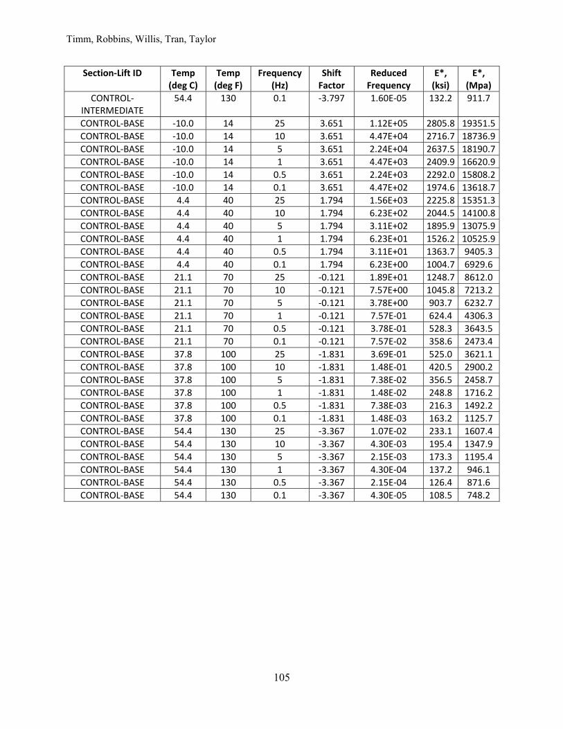
Timm, Robbins, Willis, Tran, Taylor
105
Section‐Lift ID Temp (deg C)
Temp (deg F)
Frequency (Hz)
Shift Factor
Reduced Frequency
E*, (ksi)
E*, (Mpa)
CONTROL‐INTERMEDIATE
54.4 130 0.1 ‐3.797 1.60E‐05 132.2 911.7
CONTROL‐BASE ‐10.0 14 25 3.651 1.12E+05 2805.8 19351.5
CONTROL‐BASE ‐10.0 14 10 3.651 4.47E+04 2716.7 18736.9
CONTROL‐BASE ‐10.0 14 5 3.651 2.24E+04 2637.5 18190.7
CONTROL‐BASE ‐10.0 14 1 3.651 4.47E+03 2409.9 16620.9
CONTROL‐BASE ‐10.0 14 0.5 3.651 2.24E+03 2292.0 15808.2
CONTROL‐BASE ‐10.0 14 0.1 3.651 4.47E+02 1974.6 13618.7
CONTROL‐BASE 4.4 40 25 1.794 1.56E+03 2225.8 15351.3
CONTROL‐BASE 4.4 40 10 1.794 6.23E+02 2044.5 14100.8
CONTROL‐BASE 4.4 40 5 1.794 3.11E+02 1895.9 13075.9
CONTROL‐BASE 4.4 40 1 1.794 6.23E+01 1526.2 10525.9
CONTROL‐BASE 4.4 40 0.5 1.794 3.11E+01 1363.7 9405.3
CONTROL‐BASE 4.4 40 0.1 1.794 6.23E+00 1004.7 6929.6
CONTROL‐BASE 21.1 70 25 ‐0.121 1.89E+01 1248.7 8612.0
CONTROL‐BASE 21.1 70 10 ‐0.121 7.57E+00 1045.8 7213.2
CONTROL‐BASE 21.1 70 5 ‐0.121 3.78E+00 903.7 6232.7
CONTROL‐BASE 21.1 70 1 ‐0.121 7.57E‐01 624.4 4306.3
CONTROL‐BASE 21.1 70 0.5 ‐0.121 3.78E‐01 528.3 3643.5
CONTROL‐BASE 21.1 70 0.1 ‐0.121 7.57E‐02 358.6 2473.4
CONTROL‐BASE 37.8 100 25 ‐1.831 3.69E‐01 525.0 3621.1
CONTROL‐BASE 37.8 100 10 ‐1.831 1.48E‐01 420.5 2900.2
CONTROL‐BASE 37.8 100 5 ‐1.831 7.38E‐02 356.5 2458.7
CONTROL‐BASE 37.8 100 1 ‐1.831 1.48E‐02 248.8 1716.2
CONTROL‐BASE 37.8 100 0.5 ‐1.831 7.38E‐03 216.3 1492.2
CONTROL‐BASE 37.8 100 0.1 ‐1.831 1.48E‐03 163.2 1125.7
CONTROL‐BASE 54.4 130 25 ‐3.367 1.07E‐02 233.1 1607.4
CONTROL‐BASE 54.4 130 10 ‐3.367 4.30E‐03 195.4 1347.9
CONTROL‐BASE 54.4 130 5 ‐3.367 2.15E‐03 173.3 1195.4
CONTROL‐BASE 54.4 130 1 ‐3.367 4.30E‐04 137.2 946.1
CONTROL‐BASE 54.4 130 0.5 ‐3.367 2.15E‐04 126.4 871.6
CONTROL‐BASE 54.4 130 0.1 ‐3.367 4.30E‐05 108.5 748.2

Timm, Robbins, Willis, Tran, Taylor
106
APPENDIX E – IDT CREEP COMPLIANCE DATA
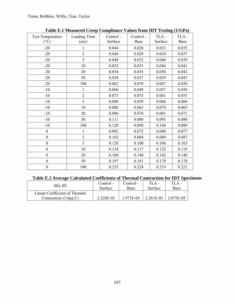
Timm, Robbins, Willis, Tran, Taylor
107
Table E.1 Measured Creep Compliance Values from IDT Testing (1/GPa) Test Temperature
(°C) Loading Time
(sec) Control - Surface
Control - Base
TLA - Surface
TLA - Base
-20 1 0.044 0.028 0.033 0.035
-20 2 0.046 0.029 0.034 0.037
-20 5 0.048 0.032 0.040 0.039
-20 10 0.052 0.033 0.044 0.041
-20 20 0.054 0.035 0.050 0.043
-20 50 0.058 0.037 0.059 0.047
-20 100 0.062 0.039 0.067 0.050
-10 1 0.066 0.049 0.057 0.050
-10 2 0.073 0.053 0.061 0.053
-10 5 0.080 0.059 0.068 0.060
-10 10 0.088 0.063 0.074 0.065
-10 20 0.096 0.070 0.081 0.071
-10 50 0.111 0.080 0.093 0.080
-10 100 0.120 0.090 0.104 0.089
0 1 0.092 0.072 0.080 0.077
0 2 0.102 0.084 0.089 0.087
0 5 0.120 0.100 0.106 0.103
0 10 0.134 0.117 0.122 0.118
0 20 0.160 0.140 0.142 0.140
0 50 0.197 0.181 0.179 0.178
0 100 0.235 0.224 0.219 0.221
Table E.2 Average Calculated Coefficients of Thermal Contraction for IDT Specimens
Mix ID Control - Surface
Control - Base
TLA - Surface
TLA - Base
Linear Coefficient of Thermal Contraction (1/deg C) 2.228E-05 1.971E-05 2.261E-05 2.075E-05