1

Mutual Fund Style Analysis: A Stochastic Dominance Approach

Jue Ren∗

17th August 2017

Abstract

It is a well-known fact that actively managed mutual funds on average underperform pass-

ive benchmarks. In this paper, we use the stochastic dominance test proposed by Linton,

Maasoumi, and Whang (2005) to shed new light on mutual fund performance on average and

across styles. This test evaluates mutual fund performance using a non-parametric framework

that 1) imposes a minimal set of conditions on preferences; and 2) analyzes the entire return

distribution for each mutual fund group. We find little evidence that actively managed mutual

funds on average underperform the passive benchmark, suggesting that mutual fund perform-

ance results are highly sensitive to investor preference assumptions. Exploring the returns for

different styles of mutual funds, we find that aggressive mutual funds underperform the mar-

ket for risk-averse investors, whereas both growth & income and income funds outperform the

market for prudent investors. Furthermore, we find that mutual fund portfolios formed by the

stochastic dominance approach provide superior future performance.

Key Words: Mutual Fund, Stochastic Dominance, Performance Evaluation

JEL Classification: C12,C15,G11

∗Jue Ren is from Department of Finance, M. J. Neeley School of Business, Texas Christian University,Fort Worth, TX 76129, United States. E-mail address: jue.ren@tcu.edu.

2

1 Introduction

Mutual funds are one of the fastest growing financial intermediaries in the United States. The

industry has grown in size to 16 trillion dollars and attracts over 40 percent of U.S. households

as investors. It is the second largest type of financial intermediary in the United States,

falling just short of commercial banks.1 However, there has been a debate about whether

or not actively managed mutual fund managers add value. The answer to this questions

is crucial for investors’ asset allocation decisions and asset managers’ investment strategies.

Academics find that the growth in actively managed U.S. equity mutual funds is puzzling

since numerous studies have shown that, post fees, these funds provide investors with average

returns significantly below those on passive benchmarks.2 While most previous research

concludes that actively managed mutual funds underperform the market when comparing

the mean and standard deviation of returns, this paper asks two questions: 1) Can some

omitted risk factors or investors’ preferences explain the puzzle? 2) Do some styles of actively

managed mutual funds perform better than others or better than the market?

Investors and academic researchers have a long-standing interest in return and risk

tradeoff. The Sharpe ratio, which is defined as the ratio of excess return to volatility, is

one of the most common measures of portfolio performance. Sharpe (1966) developed it as

a tool for mutual fund performance evaluation. However, Goetzmann, Ingersoll, and Spiegel

(2007) point out that a dynamic levering strategy, which involves increasing leverage after a

period of poor returns or decreasing leverage after a period of good returns, could increase

the Sharpe ratio. The manipulation of the Sharpe ratio consists largely in selling the upside

return potential, thus creating a distribution with high left-tail risk. A significant restriction

on the applicability of the Sharpe ratio results from the facts that: 1) It assumes a quadratic

utility function; and 2) It utilizes only the first two moments of the return distributions.

1See the 2015 Investment Company Fact Book at https://www.ici.org/pdf/2015 factbook.pdf.2See for example, Jensen (1968), Lehmann and Modest (1987), Grinblatt and Titman (1989, 1993), Elton,

Gruber, Das, and Hlavka (1993), Brown and Goetzmann (1995), Malkiel (1995), Gruber (1996), Carhart(1997), Edelen (1999), Wermers (2000), Pastor and Stambaugh (2002), Gil-Bazo and Ruiz-Verdu (2009),Fama and French (2010), Elton, Gruber, and Blake (1996, 2003, 2011), and others.

3

When the underlying data appear to follow a normal distribution, quadratic preferences will

not miss anything by only considering mean and variance. However, it is well-known that

the distributions of financial returns deviate significantly from normality.3 Thus, variance is

inadequate as the only quantifier of risk in mutual fund performance evaluation.

High distribution moments have received notable attention after the recent financial tur-

moil. A growing body of research reveals that investors favor right skewness,4 and do not

like tail risk or rare disaster risk.5 Sortino and Price (1994), Dowd (2000), and Kadan and

Liu (2014) propose performance measures that account for the higher moments of the dis-

tribution. In this paper, we study a performance measure that not only accounts for higher

moments of the distribution but also imposes a minimal set of conditions on investors’ pref-

erences.

This paper uses a stochastic dominance (SD) approach to test if mutual funds on average

underperform as a group and if particular styles of mutual funds underperform. The main

advantages of the stochastic dominance approach are that it imposes a minimal set of con-

ditions on investors’ preferences and the underlying return distributions. These conditions

consist of degree of risk aversion, preference for skewness, and an aversion to kurtosis. For

a rational agent with a known utility function, one group of mutual funds is preferred if it

maximizes expected utility, which works in theory. However, in practice it is often difficult

to find an investor’s utility function. Therefore, it would be most useful to know whether

or not a certain group of mutual funds is the dominant choice because it is preferred by all

agents whose utility functions share certain general characteristics.

To implement the stochastic dominance approach, we examine various levels of stochastic

dominance between the returns on mutual fund groups and the passive benchmark. The rules

3For example, Mandelbrot (1963) and Breen and Savage (1968) have shown that stock price changes areinconsistent with the assumption of normal probability distributions.

4See for example, Kraus and Litzenberger (1976), Jean (1971), Kane (1982), Harvey and Siddique (2000),Zhang (2005), Smith (2007), Brunnermeier, Gollier, and Parker (2007), Boyer, Mitton, and Vorkink (2010),Kumar (2009), and others.

5See for example, Barro (2009), Gabaix (2008), Gourio (2012), Chen, Joslin, and Tran (2012), Wachter(2013), and others.

4

for first order stochastic dominance (FSD) state the necessary and sufficient conditions under

which one asset is preferred to another by all expected utility maximizers. The rules for

second order stochastic dominance (SSD) state the necessary and sufficient conditions under

which one asset is preferred to another by all risk-averse expected utility maximizers. The

rules for third order stochastic dominance (TSD) state the necessary and sufficient conditions

under which one asset is preferred to another by all prudent (increasing risk aversion) risk-

averse expected utility maximizers. If there is no dominance relationship between different

classes of mutual funds and the passive benchmark, it suggests that investors with different

utility functions will have different preferences over mutual funds and the passive benchmark.

If the passive benchmark was to dominate certain mutual fund groups at the first order (or

second order), it would mean that all expected utility maximizers (risk-averse investors)

prefer the passive benchmark to certain classes of mutual funds. This outcome would be

quite puzzling. Why would investors continue to pour money into actively managed funds

despite the fact that they prefer the distribution of the passive benchmark?

Using a stochastic dominance approach, which imposes a minimal set of conditions on

investors’ preferences and the underlying return distributions, we find little evidence that

actively managed mutual funds on average underperform the passive benchmark. Although

aggressive mutual funds underperform the market for risk-averse investors, there is some

evidence showing that both growth & income as well as income funds outperform the market

for prudent investors. These results indicate the importance of considering investors’ utility

functions when analyzing investor behavior.

To implement the stochastic dominance approach, we first compare the return distribu-

tions between the mutual funds and the passive benchmark. We adopt value-weighted returns

of all stocks listed on the NYSE, AMEX, or NASDAQ (market) as the passive benchmark for

comparison. Over the period of 1980 to 2015, there is no evidence of a first order stochastic

dominance relationship between the mutual funds and the market. This indicates that ex-

pected utility maximizers do not all prefer either mutual funds or the passive benchmark.

5

Similarly, there is no evidence of a second order or third order stochastic dominance relation-

ship between the mutual funds and the market. These results show that there is no uniform

preference between the mutual funds and the market for all risk-averse investors nor for all

prudent investors as well.

Second, we examine whether some styles of mutual funds perform better than others

or than the market. Mutual funds attempt to differentiate their services by specializing

in certain sectors of the stock market. Chen, Jegadeesh, and Wermers (2000) point out

that growth funds claim to specialize in the “glamour” or low book-to-market stocks, while

income funds claim to specialize in “value” or high book-to-market stocks. We analyze

whether such specialization adds value to investors and whether some styles of actively

managed mutual funds perform better than others or better than the market. We analyze

the return distribution of four classes of mutual fund investment objectives (aggressive,

growth, growth & income, and income). After deducting management fees, we find that the

market dominates the aggressive fund by second order stochastic dominance from 1980 to

2015. This suggests that all risk-averse investors prefer the market over average aggressive

funds. The result confirms that it is indeed puzzling why risk-averse individuals would invest

in aggressive funds. However, it is possible that the major flow to aggressive funds is made

by investors with certain non-concave utility functions.

Surprisingly, there is some evidence showing that both income and growth & income funds

dominate the market by third order dominance before and also after fees are deducted.

In addition, the SD results show that income and growth & income funds dominate the

market by second order dominance during economic recessions. This result is consistent

with the findings in Moskowitz (2000), Kosowski (2006) and Glode (2011): active mutual

funds perform better in recessions and are therefore potentially desirable relative to passive

benchmarks.

Third, we calculate the risk adjusted return based on a four-factor model in order to

further compare the performance among different classes of mutual funds. Using a four-

6

factor model, a number of previous studies document that the typical actively managed U.S.

equity fund earns a negative alpha after fees (Gruber (1996), Carhart (1997), French (2008),

and Fama and French (2010)). We confirm this finding in our risk adjusted return estimation

as well. After controlling for the market risk premium, size, value, and momentum factors,

the risk adjusted return of aggressive funds is dominated by all of the other three classes of

mutual funds by second order stochastic dominance. In addition, growth & income funds

dominate all of the other three classes of mutual funds by second order stochastic dominance.

Overall, our results indicate that SD tests provide a robust analysis of mutual fund

performance. From a broader perspective, there are two important issues for investors to

consider when selecting mutual funds: whether a superior mutual fund can be identified in

advance and whether there is persistence in performance. A number of empirical studies

demonstrate that the relative performance of equity mutual funds persists from period to

period.6

Finally, we examine whether ex-post SD relationships provide exploitable information

on ex-ante returns. We construct mutual fund portfolios based on second order stochastic

dominance. At the beginning of each year between 1995-2015, we identify the dominated

(second order) mutual funds based on the most recent sixty monthly returns. We then form

an equal weighted portfolio of these dominated mutual funds, which is rebalanced annually.

The results show that portfolios formed by a stochastic dominance approach deliver better

performance than mean-variance efficient portfolios.

Although a number of studies have used a stochastic dominance approach to rank re-

turn distributions in the finance literature, most of these SD tests do not take the depend-

ence structure of financial returns into account. Lean, Phoon, and Wong (2011) employ

a stochastic dominance approach to rank the performance of commodity trading advisers’

funds. Seyhun (1993) uses a stochastic dominance approach to test for the existence of the

January effect. The critical value of stochastic dominance tests in these two studies require

6Carhart (1997), Brown and Goetzmann (1995), Busse and Irvine (2006), and Elton, Gruber, and Blake(1996, 2011).

7

an i.i.d assumption for returns. However, Fung and Hsieh (1997) and Brown and Goetzmann

(1995) show mutual fund returns are highly correlated and this cross-fund correlation issue

should be addressed. In this paper, we have adopted the Linton, Maasoumi, and Whang

(LMW) test, which can accommodate not only the general dependence between mutual fund

returns, but also the serial dependence.

We describe our data in detail in Section II. Section III introduces the stochastic domin-

ance test, and Section IV discusses the hypotheses and test statistics. Empirical results are

provided in Section V. Section VI discusses robustness tests and Section VII concludes.

2 Data

Our sample builds upon two data sets. We begin with a mutual fund sample from the CRSP

(Center for Research in Security Prices) Survivorship-Bias-Free Mutual Funds database.

The database includes information on funds’ returns, fees, investment objectives (style), and

size (total net assets). In this study, we limit our analysis to actively managed domestic

equity mutual funds between March 1980 and December 2015, which contains the most

complete and reliable return data.7 Specifically, we include only mutual funds that have

a self-declared investment objective of “MCG,” “AGG,” “CA,” “G,” “LTG,” “GRO,” “IEQ,”

“OPI,”“EI,”“GCI,”“GRI,” or “GI.”

We follow Kacperczyk, Sialm, and Zheng (2008) in eliminating balanced, bond, money

market, international, sector, and index funds. We mainly use CRSP objective codes to

classify the mutual funds into four investment classes (aggressive, growth, growth & income,

and income). As shown in Table 1, we classify mutual funds with the objective of “Max-

7Fama and French (2010) state that there is a potential problem in the CRSP mutual fund return dataduring the period 1962 to 1983. For this time period, about 15% of the funds on the CRSP report onlyannual returns, and the average annual equal-weight (EW) return for these funds is 5.29% lower than forfunds that report monthly returns. Also, MFLINKS data starts in March 1980. Given the nature of ourtests and data availability, we choose the sample period from March 1980 to December 2015.

8

imum Capital Gains,” “Equity USA Aggressive Growth,” or “Capital Appreciation Funds”

as aggressive funds; mutual funds with the objective of “Growth,”“Long-Term Growth,” or

“Equity USA Growth” as growth funds; mutual funds with the objective of “Equity Income,”

“Option Income,” or “Equity Income Funds” as income funds; and mutual funds with the

objective of “Growth and Current Income,”“Equity USA growth & income,”“Equity USA

Income &Growth,” or “Growth and Income Funds” as growth & income funds.

Some mutual funds have multiple share classes. The CRSP data lists each share class as a

separate fund. Different share classes have the same holding compositions and typically differ

only in fee structure. The returns histories are therefore sometimes duplicated in the CRSP

dataset. For example, if a fund started in 1983 and split into four share classes in 1993, each

new share class of the fund is permitted to inherit the entire return history. This can create

a bias when averaging returns across mutual funds. For funds with multiple share classes, we

use the identification code in MFLINKS to combine different classes of the same fund into

a single value-weighted fund. Wermers (2000) provides a description of how MFLINKS are

created. Each monthly fund return is computed by weighting the return of its component

share classes by their beginning-of-month total net asset values.

We obtain monthly data for the size, value, momentum, and market portfolios for the

period of 1980 to 2015 from Kenneth French’s data library. We measure recessions using

the definition of the National Bureau of Economic Research (NBER) business cycle dating

committee. The start of the recession is the peak of economic activity and its end is the

trough. Our aggregate sample spans 430 months of data from March 1980 until December

2015, among which 55 are NBER recession months (13%).

9

3 Stochastic Dominance

This section provides a non-parametric approach based on stochastic dominance testing to

evaluate mutual fund performance. The theory of stochastic dominance offers a decision-

making rule under uncertainty provided the decision maker’s utility function has certain

properties. The different orders of stochastic dominance correspond to increasing restrictions

on the shape of the utility function and the agents’ attitude towards higher order moments.

These restrictions are non-parametric and do not require specific parametric function forms.

We first briefly define the criteria of stochastic dominance:

1. First order stochastic dominance: When A dominates B by first order stochastic dom-

inance, all expected utility maximizers (u′ ≥ 0) prefer A to B.

2. Second order stochastic dominance: When A dominates B by second order stochastic

dominance, all risk-averse expected utility maximizers (u′ ≥ 0, u′′ ≤ 0) prefer A to B.

3. Third order stochastic dominance: When A dominates B by third order stochastic

dominance, all prudent risk-averse expected utility maximizers (u′ ≥ 0, u′′ ≤ 0, u′′′ ≥

0) prefer A to B.

We use X1 and X2 to denote two random variables (e.g., mutual fund returns and market

returns). Let U1 denote the set of von Neumann-Morgenstern type utility functions, u, such

that u′ ≥ 0 (more is better than less). Let U2 denote the set of utility functions in U1

for which u′′ ≤ 0 (concavity). Let U3 denote the class of all utility functions in U2 for

which u′′′ ≥ 0 (increasing risk aversion). Let F1(x) and F2(x) be the cumulative distribution

functions, respectively.

Then define the following:

10

Definition 1: X1 first order stochastic dominates X2, denoted X1 �FSD X2, if and only

if:

E[u(X1)] ≥ E[u(X2)] for all u ∈ U1 with strict inequality for some u; or

F1(x) ≤ F2(x) for all x with strict inequality for some x.

Definition 2: X1 second order stochastic dominates X2, denoted X1 �SSD X2, if and

only if:

E[u(X1)] ≥ E[u(X2)] for all u ∈ U2 with strict inequality for some u; or´ x−∞ F1(t)dt ≤

´ x−∞ F2(t)dt for all x with strict inequality for some x.

Definition 3: X1 third order stochastic dominates X2, denoted X1 �TSD X2, if and only

if:

E[u(X1)] ≥ E[u(X2)] for all u ∈ U3 with strict inequality for some u; or´ x−∞

´ z−∞ F1(t)dtdz ≤

´ x−∞

´ z−∞ F2(t)dtdz for all x with strict inequality for some x.

Mathematically, lower order dominance implies all higher order dominance rankings. In

the case of first order dominance, the distribution function of X1 lies everywhere to the right

of the distribution function of X2 except for a finite number of points where there is strict

equality. For first order stochastic dominance, the probability that returns of X1 are in excess

of r is higher than the corresponding probability associated with X2.

Pr(X1 > r) ≥ Pr(X2 > r).

An important feature of the definitions of stochastic dominance is that they impose min-

imum conditions on the preferences of agents within the class of von Neumann–Morgenstern

utility functions. Stochastic dominance is more satisfactory than the commonly used mean-

variance rule since it is defined with reference to a much larger class of utility functions

11

and return distributions. Levy (2006) provides an example showing that the mean-variance

approach produces an inaccurate evaluation result. Suppose that X1 ∈ {1, 2} has equal

probability on each outcome and that X1 ∈ {2, 4} also has equal probability on each out-

come. Then E(X1) < E(X2), but var(X1) < var(X2), so that there exists a mean-variance

optimizer who prefers X1 over X2. However, this does not make economic sense because

X1 ≤ X2 with a probability of one. X1 is first order stochastic dominated by X2.

4 Hypotheses and Test Statistics

X1 denotes the average actively managed mutual fund return; X2 denotes the market

return; X3 denotes the aggressive fund return; X4 denotes growth fund return; X5 denotes

growth and income fund return; and X6 denotes income fund return. The hypothesis tested

is whether or not one group of mutual funds or the market dominates the other. We examine

the stochastic dominance relationship between all pairs of returns of Xk for k = 1 . . . 6. One

example of the type of test we conduct is:

H0: The market stochastically dominates average actively managed mutual fund,

with the alternative being that there is no stochastic dominance.

Next, we formalize these tests. Let χ denote the support of Xk for k = 1 . . . 6 and let

s = 1, 2, 3 represent the order of stochastic dominance. Define:

FK(x) = P (X ≤ x), (1)

D(1)K (x) = FK(x), (2)

12

D(s)K (x) =

xˆ

−∞

D(s−1)K (t)dt for s ≥ 2. (3)

We say that Xk stochastically dominates Xl at order s, if D(s)k (x) ≤ D

(s)l (x) for all x with

strict inequality for some x.

For each k = 1 . . . 6; s = 1, 2, 3, and x ∈ χ, let D(s)kl = D

(s)k (x)−D(s)

l (x). Define:

d∗s = maxk 6=lsupx∈χ

[D

(s)kl

]. (4)

As Klecan, McFadden, and McFadden (1991) suggests, the hypothesis of interest can be

stated as:

H0 : d∗s ≤ 0 vs. Ha : d∗s > 0. (5)

The test statistics are based on the empirical analogues of d∗s. We define the test statistics

as:

D(s)N = maxk 6=lsupx∈χ

√N

[D

(s)kl (x)

], (6)

where

D(s)k (x) =

1

N(S − 1)!

N∑i=1

(x−Xki)s−11(Xki ≤ x) for k = 1, ..., 6. (7)

We adopt a recentering function to account for the effect of the parameter estimation

error as suggested in Donald and Hsu (2013). Simulation results in Donald and Hsu (2013)

show that the recentering function increases the power of the test. For a given small negative

number aN , define the recentering function as µ = (Fk(x)−Fl(x))∗1(√N(Fk(x)−Fl(x)) < aN.

We next describe the main method for obtaining critical values: the subsampling ap-

proach. Klecan, McFadden, and McFadden (1991) point out that even when the data are

13

i.i.d in stochastic dominance testing, the standard bootstrap method does not work because

one needs to impose the null hypothesis in that case. The mutual dependence of the fund

returns as well as the time series dependence in the data make it challenging to obtain

consistent critical values. As Linton, Maasoumi, and Whang (2005) suggest, we use the

subsampling method to obtain a consistent critical value.

In order to define the subsampling procedure, let Wi = {Xki : k = 1, 2, 3, 4, 5, 6}for i =

1...N . TN denotes the test statistics D(s)N . We first generate the subsamples of size b by taking

without replacement from the original data. There will be N − b + 1 different subsamples

of size b. We then compute the test statistics tN,b,i using subsamples {Wi,Wi+1, . . . ,Wi+b−1}

for i = 1, 2, ..., N − b+ 1. Linton, Maasoumi, and Whang (2005) show that this subsampling

procedure works under a very weak condition on b and is data-dependent. The sampling

distribution GN of TN can be approximated by:

GN,b(w) =1

N − b+ 1

N−b+1∑i=1

1(√btN,b,i ≤ w). (8)

gN.b(1− α) is the (1− α)th sample quantile of GN,b(w). We reject the null at significant

level α if Tn > gN.b(1− α).

5 Results

5.1 Summary Data on Mutual Funds

Table 2 reports the summary statistics for our actively managed mutual fund sample.

There are a total of 2,666 mutual funds in our sample, which are divided into four categories

as previously discussed. Aggressive funds attempt to achieve the highest capital gains and

the investments held in these funds are companies that demonstrate high growth potential,

usually accompanied by a large amount of share price volatility. Growth funds invest in

growth companies with the primary aim of achieving capital gains instead of dividend in-

14

come. Income funds seek to provide a high current income by investing in high-yielding

conservative stocks. Growth & income funds seek to provide both capital gains and a steady

stream of income. In Panel A, we report the gross returns, net returns, skewness, kurtosis,

autocorrelation, and Sharpe ratio for equal weighted mutual fund groups. Gross return is

defined as the mutual funds’ return before deducting any management fees. Net return is

the return received by investors. Consistent with what the previous literature has found, the

average returns of all five mutual fund groups are lower than the market. The standard de-

viation for more conservative funds is lower. All mutual fund groups’ return and the market

return are negatively skewed. All the returns series have some serial dependence based on the

autocorrelation statistics. In Panel B, we report similar statistics for value-weighted mutual

fund groups. Panel C shows that all of the returns of the mutual fund groups are highly

correlated. Thus, the LMW stochastic dominance test is used because it accommodates not

only general dependence between returns, but also serial dependence.

5.2 Normality Test

When the underlying variable is normal, the traditional performance evaluation meas-

ure will not miss anything by only considering mean and variance. However, one issue in

performance evaluation is that the returns of mutual funds are non-normal. Table 3 shows

the Kolmogorov-Smirnov and Jarque-Bera test results. For any group of mutual funds, the

normality hypothesis is strongly rejected. Previous literature has also documented non-

normalities in mutual fund returns. Kosowski, Timmermann, Wermers, and White (2006)

suggest these non-normalities arise for three reasons. First, individual stocks within a typ-

ical mutual fund portfolio realize returns with non-negligible higher moments and managers

often hold heavy positions in relatively few stocks or industries. Second, individual stocks

exhibit varying levels of time-series autocorrelations in returns. Third, funds may imple-

ment dynamic strategies that involve changing their levels of risk-taking when the risk of

the overall market portfolio changes. Kosowski, Timmermann, Wermers, and White (2006)

15

argue that normality may be a poor approximation in practice, even for a fairly large mutual

fund portfolio. The stochastic dominance test is based on the entire distribution. Unlike the

Sharpe ratio, it does not require the return to be normally distributed.

5.3 Mutual Funds and Market Return Comparison

Stochastic dominance tests implicitly take into account the differences in expected returns

and risk. While traditional performance evaluation tools take the standard deviation as

a quantifier for risk, the stochastic dominance approach will consider standard deviation,

skewness, kurtosis, and all higher moments for the evaluation. For example, we are interested

in comparing asset A and asset B for investors with general utility assumptions. If asset A

has a higher expected return than asset B, then asset A will be preferred if we only consider

the mean and ignore the risk. However, if the higher expected return of asset A is due to

its higher risk, then asset A would exhibit more extreme positive and negative returns. For

investors with various preferences for risk and return trade-off, asset A may or may not be

preferred. Thus, asset A will not stochastically dominate asset B.

In this section, we apply the stochastic dominance test to compare the distributions of

monthly market returns and mutual fund returns. Figure 1 shows the cumulative density

function (CDF) of the realized equal weighted actively managed mutual fund returns and

market returns from 1980-2015 and Figure 2 shows the CDF of the realized value-weighted

actively managed mutual fund returns and market returns for the same time period. Inspec-

tion of the graph suggests no evidence of first order stochastic dominance as the two CDFs

cross.

Table 4 summarizes the stochastic dominance test results for equal weighted mutual

funds and the market. In Panel A, we test for stochastic dominance between the market and

mutual fund net returns. In Panel B, we test for stochastic dominance between the market

and mutual fund gross returns. The first column of Table 4 lists the return pairs we are

testing. The null hypothesis is that the first return series will stochastically dominate the

16

second return series. For example, “Average Mutual Fund vs. Market” means that we test

whether or not the equal-weighted average of mutual fund returns stochastically dominate

the market. In the second column, we list the order of stochastic dominance being tested.

The test statistics are given in the third column. The final three columns provide the p-value

calculated from a different subsample block size.

The test statistics of FSD in Panel A of Table 4 has a value of 0.27 with a p-value of

0.00. As expected from Figure 1, the market returns do not dominate the average actively

managed fund net returns by first order stochastic dominance. This implies that expected

utility maximizers do not all prefer either actively managed mutual funds or the market

benchmark. The test value of SSD in Panel A has a value of 0.01, with a p-value of 0.00,

showing that there is also no evidence of second order stochastic dominance between the

two assets. This implies that risk-averse investors do not all prefer either actively managed

mutual funds or the market benchmark. The test value of TSD in Panel A is positive and

shows no evidence of third order stochastic dominance between two assets. This implies that

prudent investors also do not all prefer either actively managed mutual funds or the market

benchmark.

Panel B of Table 4 shows the SD test results for the market and actively managed mutual

fund gross returns. Even without deducting any management fees, there is still no evidence

of a dominance relationship between two assets. The SD test statistics are all positive with

p-values less than 5%.

Overall, the results in Table 4 show no stochastic dominance relationship between average

actively managed mutual fund returns and the market returns by first order, second order,

or third order stochastic dominance. The SD test statistics are all positive with p-values less

than 5%. This suggests that investors with certain utility functions prefer the distribution

of the market returns, while some other investors with different utility functions prefer the

return distribution of actively managed mutual funds. The test results here reveal that

investors’ utility functions will play a role in evaluating the return distribution of actively

17

managed funds and the market.

5.4 Investment Objective Subgroups of Mutual Funds and Market

Return Comparison

Mutual funds have attempted to differentiate their services by specializing in certain

sectors of the stock market and adopting various investment styles. For example, growth

funds claim to specialize in low book-to-market stocks, while income funds claim to specialize

in high book-to-market stocks. The question is whether such specialization adds value to

investors. We investigate this issue by partitioning funds based on their self-declared invest-

ment objectives (aggressive, growth, income, and growth & income). In this Section, we use

a stochastic dominance approach to examine whether some styles of mutual funds perform

better than others or better than the market. Figure 2 and Figure 3 plot the CDF of four

classes of mutual fund and the market returns. Once again, all of the CDFs cross, so we do

not expect to find first order stochastic dominance.

Table 5 summarizes the stochastic dominance results for the four mutual fund classes and

the market both before and after management fees have been deducted. Before deducting

management fees, aggressive funds are third order stochastically dominated by each of the

other three classes of mutual funds and also the market. After deducting management fees,

aggressive funds are still third order dominated by each of the other three classes of mutual

funds and second order dominated by the market. This test result shows that aggressive

funds on average are inferior to the other three mutual fund classes and the market for all

prudent investors with or without considering management fees. Also, on a net return basis,

all risk-averse investors prefer the market to average aggressive funds. The underperformance

of aggressive funds is not surprising given the high exposure to market risk and high betas.

Hong and Sraer (2016) provide a theory for why high beta assets are prone to speculative

overpricing. They point out that when investors disagree about the stock market’s prospects,

18

high beta assets are more sensitive to this aggregate disagreement. Thus, high beta assets

experience a greater divergence of opinion about their payoffs and are overpriced due to short-

sales constraints. The stochastic test result confirms that risk-averse individuals do not prefer

aggressive funds. This suggests that the major flow to aggressive funds is probably made by

investors with certain non-concave utility functions.

The absence of second order stochastic dominance between income funds and the market

means that certain risk-averse individuals (e.g., those with quadratic utility functions) prefer

the income fund, while some other risk-averse individuals with different utility functions

prefer the market return. This result is in contrast to the Sharpe ratio result, presented

in the summary statistics table, which posits that the income fund (Sharpe ratio 14.26) is

preferred to the market (Sharpe ratio 13.98) for all agents with a quadratic utility function.

Although the Sharpe ratio also considers this risk and return trade-off with variance as the

quantifier for risk, since it ignores higher moments in the distribution, it does not provide

an accurate result for all subsets of this data. In counterpoint, the stochastic dominance

approach provides a robust analysis of the performance, which allows for differentiation

between different types of investors.

Surprisingly, there is some evidence that both growth & income funds and income funds

dominate the market by third order stochastic dominance before and also after fees. This

implies that income and growth & income will be favored for all prudent individuals who have

a preference for positive skewness and an aversion for variance and kurtosis. As shown in the

summary statistics, income and growth & income funds have slightly lower average returns

than the market. However, they both also have a lower variance, smaller negative skewness,

and smaller kurtosis. Including these measures of risk preference will therefore provide a

different picture of the fund performance evaluation. Even though these funds have lower

returns, they are also less risky. The existence of third order stochastic dominance means

that all prudent investors prefer income and growth & income funds to the market as seen

in the entire 1980-2015 monthly return distribution.

19

5.5 Recession/Boom

The early literature on the value of active mutual fund management focuses on uncondi-

tional return performance and generally finds that the average fund underperforms passive

benchmarks8 and that there is evidence of negative market timing.9 However, Moskowitz

(2000), Kosowski (2006), and Glode (2011) all suggest that unconditional mutual fund per-

formance measures may understate the value of mutual funds to investors since they cannot

answer the question of how mutual funds perform in recession states when investors’ mar-

ginal utility of wealth is highest. Their findings imply that actively managed mutual funds

perform better in recessions and are therefore potentially desirable relative to benchmarks.

In this Section, we explore the performance of mutual funds and the market during differ-

ent economics conditions. The stochastic dominance test is conducted for NBER recessions

and expansions. Our aggregate sample spans 430 months of data from March 1980 until

December 2015, among which 55 are NBER recession months (13%).

During economic expansion periods, the SD test results are very similar to what were

seen in previous Sections. First, there is no dominance relationship between average actively

managed mutual funds and the market by first order, second order, or third order stochastic

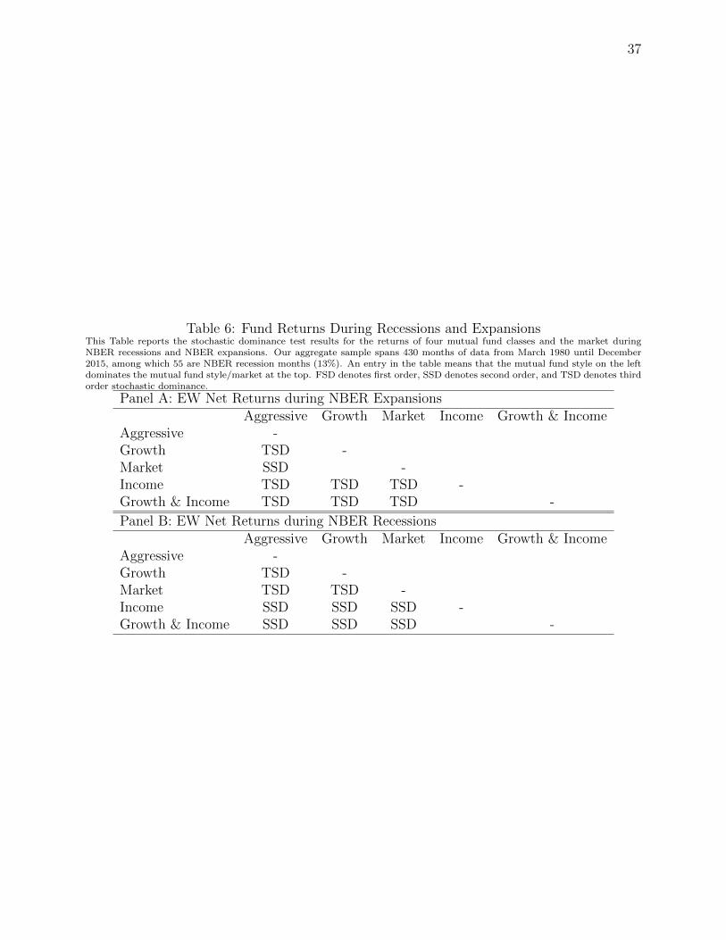
dominance during the economic expansion periods in our sample. Second, Panel A of Table 6

shows that the market still dominates aggressive funds by second order stochastic dominance

after deducting all the fees during economic expansion periods. Also, aggressive funds are

third order stochastically dominated by the other three mutual fund classes. Third, there

is evidence showing that income and growth & income funds dominate the market by third

order dominance during economic expansions.

8See for example, Jensen (1968), Lehmann and Modest (1987), Grinblatt and Titman (1989, 1993), Elton,Gruber, Das, and Hlavka (1993), Brown and Goetzmann (1995), Malkiel (1995), Gruber (1996), Carhart(1997), Edelen (1999), Wermers (2000), Pastor and Stambaugh (2002), Gil-Bazo and Ruiz-Verdu (2009),Fama and French (2010), Elton, Gruber, and Blake (1996, 2003, 2011), and others.

9

See Treynor and Mazuy (1966), Henriksson and Merton (1981), Chang and Lewellen (1984), Grinblattand Titman (1989), and Jagannathan and Korajczyk (1986) for (unconditional) market timing studies.

20

During economic recession periods, there is no dominance relationship between average

actively managed mutual funds and the market by first order, second order, and third order

stochastic doninance in our sample. Panel B of Table 6 shows the SD test results for the

four styles of mutual funds and the market during economic recession periods. Aggressive

funds are not only third order stochastically dominated by the market, but also second order

stochastically dominated by income funds and the growth & income funds. This suggests that

the underperformance of aggressive funds persist during recessions. Income and growth &

income funds dominate the market by second order stochastic dominance. This implies that

during recessions, risk-averse investors prefer growth & income funds and income funds to

the market. Thus, these funds do create some value for risk-averse investors during economic

recession periods.

5.6 Risk Adjusted Return

In order to further compare the performance among different classes of mutual funds,

we calculate the risk adjusted return based on a four-factor model as proposed in Carhart

(1997). The models use the regression framework below:

Rit −Rft = ai + bi(RMt −Rft) + siSMBt + hiHMLt +miMOMt + eit.

In this regression, Rit is the return on fund i for month t, Rft is the risk-free rate (the

one month U.S. Treasury bill rate), RMt is the market return (the return on a VW portfolio

of NYSE, Amex, and NASDAQ stocks), SMBt and HMLt are the size and value factors as

in Fama and French (1993), MOMt is Carhart’s (1997) momentum factor, ai is the average

return left unexplained by the benchmark model, and eit is the regression residual. Table 7

provides the summary statistics for all of the factors used in the regression and Table 8 shows

the regression results. Overall, mutual funds do tilt their investments more toward stocks

that match their stated objectives. Aggressive funds have more exposure to all risk factors.

It is well-known that aggressive funds tilt toward small capitalization, low book-to-market,

and momentum stocks, while the opposite holds true for income funds.

21

For each fund i, the risk-adjusted return is calculated as:

αit = Rit − βTi Zt,

where Ztis the value of factors at month t.

We next conduct an analysis of the distributions of risk adjusted returns of the mutual

funds. Table 9 shows the SD test results for risk adjusted returns based on the four-factor

model. After controlling the market risk premium, size, value, and momentum factors, the

risk adjusted returns of aggressive funds are dominated by all of the other three classes of

mutual funds by second order stochastic dominance. In addition, the risk adjusted returns

of growth & income funds dominate all of the other three classes of mutual funds by second

order stochastic dominance.

5.7 Investment Strategy

Two important issues for mutual fund investors are whether a superior mutual fund can

be identified in advance and whether the superior performance persists. Many studies have

found performance persistence in the top-ranked mutual fund groups based on past returns,

past alpha, and past Sharpe ratio.10 In this Section, we use the stochastic dominance relation-

ship as a criterion for portfolio construction. We examine whether ex-post SD relationships

provide exploitable information on ex-ante returns. This empirical exercise targets second

order stochastic dominance. At the beginning of each year between 1995-2015, we identify

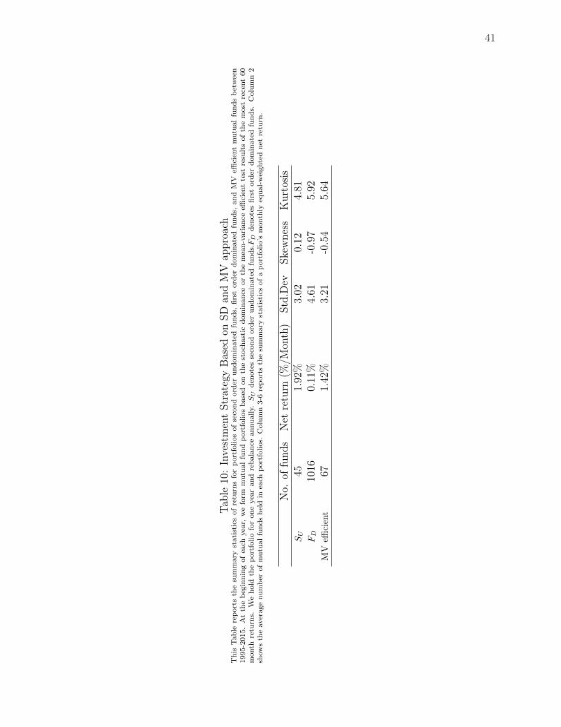
the undominated (second order) mutual funds based on the most recent 60-month returns.

We then form an equal weighted portfolio of undominated mutual funds. The portfolio is

rebalanced annually. For comparison, mean-variance efficient portfolios are formed for the

same time period.

Table 10 shows the portfolio performance based on a stochastic dominance approach and

10Carhart (1997), Busse and Irvine (2006), and Elton, Gruber, and Blake (1996, 2011).

22

a mean-variance approach. The mean return of the portfolio of second order undominated

funds is 1.92%, which is substantially larger than the portfolio of first order dominated funds.

The average return of the mean-variance efficient portfolio is 1.42%, with a 3.21 standard

deviation and negative skewness. The portfolio of second order undominated funds has a

smaller standard deviation and positive skewness compared to the mean-variance efficient

portfolio. This shows that the stochastic dominance approach may potentially be used for

mutual fund selection.

6 Robustness

6.1 Liquidity Factor

Pastor and Stambaugh (2003) show that expected stock returns are related cross-sectionally

to the sensitivities of the returns to fluctuations in aggregate liquidity. We introduce the li-

quidity factor to capture such an effect, in addition to the market, size, value, and momentum

factors. Table 11 shows the SD test results for risk adjusted returns based on a five-factor

model. The result is similar to what we have before. After controlling for the market risk

premium, size, value, momentum, and liquidity factors, the risk adjusted returns of aggress-

ive funds are dominated by all of the other three classes of mutual funds by second order

stochastic dominance. Also, the risk adjusted returns of growth & income funds dominate

all of the other three classes of mutual funds by second order stochastic dominance.

6.2 Value Weighted Portfolios

As a robustness check, we consider if our results are sensitive to the weighting method. We

perform all of the analyses again using the value-weighted mutual fund portfolios. Figure 4

plots the CDF of the net and gross return distributions of the market and the value-weighted

mutual fund portfolios. As before, the two CDFs cross and we do not expect to find a first

23

order stochastic dominance relationship. Overall, we found the results are very robust to

different weighting methods. First, Table 12 shows that there is no stochastic dominance

relationship between value-weighted mutual fund portoflios and the market, with or without

fees.

Second, the results in Table 13 show that the market still dominates aggressive funds

by second order dominance after deducting all fees. Also, aggressive funds are third order

stochastically dominated by all of the other three mutual fund classes. Third, there is

evidence showing that income and growth & income funds dominate the market by third

order dominance, with or without deducting the management fees.

Finally, Table 14 shows the SD test results for value-weighted risk adjusted returns based

on four-factor and five factor models. In both cases, the risk adjusted returns of aggressive

funds are dominated by all of the other three classes of mutual funds by third order stochastic

dominance. In addition, the risk adjusted returns of growth & income funds dominate both

growth funds and income funds by second order stochastic dominance.

7 Conclusion

Although there is no consensus on investors’ utility function form, traditional mutual fund

performance evaluation measures usually rely on a quadratic utility assumption. Moreover,

even though investors recognize the importance of the higher moments of a return distri-

bution, they generally only use variance as a risk measurement. To address this issue, this

paper evaluates mutual fund performance using a non-parametric framework that 1) imposes

a minimal set of conditions on preferences; and 2) analyzes the entire return distribution for

each mutual fund group. Previous literature finds that actively managed mutual funds on

average underperform the passive benchmark by comparing the mean and standard devi-

ation of returns. We revisit the actively managed mutual funds underperformance puzzle by

applying the stochastic dominance test proposed by Linton, Maasoumi, and Whang (2005)

24

to verify if actively managed mutual funds on average underperform and if any particular

style of actively managed mutual funds (aggressive, growth, growth & income, and income)

underperforms. The test results show little evidence that actively managed mutual funds

on average underperform the passive benchmark. This suggests that investors with different

utility functions will have different preferences over actively managed mutual funds and the

passive benchmark. Although aggressive mutual funds underperform the market for risk-

averse investors, there is some evidence showing that both growth & income and income

funds outperform the market for prudent investors. Furthermore, we find that mutual fund

portfolios formed by the stochastic dominance approach provide superior future performance.

Reference

Barro, R. J. (2009). Rare disasters, asset prices, and welfare costs. The American

Economic Review, 99(1), 243-264.

Busse, J. A., & Irvine, P. J. (2006). Bayesian alphas and mutual fund persistence. The

Journal of Finance, 61(5), 2251-2288.

Boyer, B., Mitton, T., & Vorkink, K. (2010). Expected idiosyncratic skewness. Review

of Financial Studies, 23(1), 169-202.

Breen, W., & Savage, J. (1968). Portfolio distributions and tests of security selection

models. The Journal of Finance, 23(5), 805-819.

Brown, S. J., & Goetzmann, W. N. (1997). Mutual fund styles. Journal of financial

Economics, 43(3), 373-399.

Brunnermeier, Markus K., Christian Gollier and Jonathan A. Parker. 2007. ”Optimal

Beliefs, Asset Prices, and the Preference for Skewed Returns.” American Economic Review,

97(2): 159-165.

Carhart, M. (1997), “On Persistence in Mutual Fund Performance”, The Journal of Fin-

ance, 52(1), 57-82.

25

Chang, E. C., & Lewellen, W. G. (1984). Market timing and mutual fund investment

performance. Journal of Business, 57-72.

Chen, H., Joslin, S., & Tran, N. K. (2012). Rare disasters and risk sharing with hetero-

geneous beliefs. Review of Financial Studies, 25(7), 2189-2224.

Davidson, R. and Duclos, J. (2000), “Statistical inference for stochastic dominance and

for the measurement of poverty and inequality”, Econometrica, 68, 1435-1464.

Donald, G. and Hsu, Y. (2013), “Improving the power of tests of stochastic dominance”,

working paper.

Dowd, K., (2000). Adjusting for risk: An improved Sharpe ratio. International Review

of Economics and Finance 9, 209-222

Edelen, R. M. (1999). Investor flows and the assessed performance of open-end mutual

funds. Journal of Financial Economics, 53(3), 439-466.

Elton, E. J., Gruber, M. J., Das, S., & Hlavka, M. (1993). Efficiency with costly inform-

ation: A reinterpretation of evidence from managed portfolios. Review of Financial studies,

6(1), 1-22.

Elton, E. J., Gruber, M. J., & Blake, C. R. (1996). Survivor bias and mutual fund

performance. Review of Financial Studies, 9(4), 1097-1120.

Elton, E. J., Gruber, M. J., & Blake, C. R. (2003). Incentive fees and mutual funds. The

Journal of Finance, 58(2), 779-804.

Elton, E. J., Gruber, M. J., & Blake, C. R. (2011). Holdings data, security returns,

and the selection of superior mutual funds. Journal of Financial and Quantitative Analysis,

46(02), 341-367.

Fama, Eugene F., and Kenneth R. French (1993), Common risk factors in the returns on

stocks and bonds, Journal of Financial Economics 33, 3–56.

Fama, E. F., & French, K. R. (2010). Luck versus skill in the cross-section of mutual

fund returns. The journal of finance, 65(5), 1915-1947.

Fung ,W and Hsieh,D (1997),“Empirical Characteristics of Dynamic Trading Strategies:

26

The Case of Hedge Funds” , Review of Financial Studies, 10 (1997), 275-302

Gabaix, X. (2008). Variable rare disasters: A tractable theory of ten puzzles in macro-

finance. The American Economic Review, 98(2), 64-67.

Gil-Bazo, J., & Ruiz-Verdu, P. (2009). The relation between price and performance in

the mutual fund industry. The Journal of Finance, 64(5), 2153-2183.

Glode, V. (2011). Why mutual funds “underperform”. Journal of Financial Economics,

99(3), 546-559.

Goetzmann, W., Ingersoll, J., Spiegel, M., & Welch, I. (2007). Portfolio performance

manipulation and manipulation-proof performance measures. Review of Financial Studies,

20(5), 1503-1546.

Gourio, F. (2012). Disaster risk and business cycles. The American Economic Review,

102(6), 2734-2766.

Grinblatt, M., & Titman, S. (1989). Mutual fund performance: An analysis of quarterly

portfolio holdings. Journal of business, 393-416.

Grinblatt, M., & Titman, S. (1993). Performance measurement without benchmarks: An

examination of mutual fund returns. Journal of Business, 47-68.

Gruber, M. J. (1996). Another puzzle: The growth in actively managed mutual funds.

The journal of finance, 51(3), 783-810.

Harvey, C. R., & Siddique, A. (2000). Conditional skewness in asset pricing tests. The

Journal of Finance, 55(3), 1263-1295.

Henriksson, R. D., & Merton, R. C. (1981). On market timing and investment per-

formance. II. Statistical procedures for evaluating forecasting skills. Journal of business,

513-533.

Hong, H., & Sraer, D. A. (2016). Speculative betas. The Journal of Finance.

Jean, W. H. (1971). The extension of portfolio analysis to three or more parameters.

Journal of Financial and Quantitative Analysis, 6(01), 505-515.

Jagannathan, R., & Korajczyk, R. A. (1986). Assessing the market timing performance

27

of managed portfolios. Journal of Business, 59(2), 217-235.

Jegadeesh, N. and Titman, S. (1993), “Returns to Buying Winners and Selling Losers:

Implications for Stock Market Efficiency”, The Journal of Finance, 48(1), 56-91.

Jensen, M. C. (1968). The performance of mutual funds in the period 1945–1964. The

Journal of finance, 23(2), 389-416.

Kadan, O., & Liu, F. (2014). Performance evaluation with high moments and disaster

risk. Journal of Financial Economics, 113(1), 131-155.

Kane, A. (1982). Skewness preference and portfolio choice. Journal of Financial and

Quantitative Analysis, 17(01), 15-25.

Kosowski, R., Timmermann, A., Wermers, R., & White, H. (2006). Can mutual fund

“stars” really pick stocks? New evidence from a bootstrap analysis. The Journal of finance,

61(6), 2551-2595.

Kacperczyk, M., Sialm, C., & Zheng, L. (2008). Unobserved actions of mutual funds.

Review of Financial Studies, 21(6), 2379-2416.

Kraus, A., & Litzenberger, R. H. (1976). Skewness preference and the valuation of risk

assets. The Journal of Finance, 31(4), 1085-1100.

Kumar, A. (2009). Who gambles in the stock market?. The Journal of Finance, 64(4),

1889-1933.

Klecan, L., McFadden, R., & McFadden, D. (1991). A robust test for stochastic domin-

ance. Unpublished paper, MIT.

Linton, O., E. Maasoumi and Y.-J. Whang (2005), “Consistent Testing for Stochastic

Domi- nance under General Sampling Schemes,” Review of Economic Studies 72, 735-765.

Lean, H. H., Phoon, K. F., & Wong, W. K. (2013). Stochastic dominance analysis of

CTA funds. Review of Quantitative Finance and Accounting, 40(1), 155-170.

Lehmann, B. N., & Modest, D. M. (1987). Mutual fund performance evaluation: A

comparison of benchmarks and benchmark comparisons. The journal of finance, 42(2), 233-

265.

28

Mandelbrot, B. (1967). The variation of some other speculative prices. The Journal of

Business, 40(4), 393-413.

Moskowitz,T. (2000), “Mutual fund performance: an empirical decomposition into stock-

picking talent, style, transaction costs, and expenses: discussion” ,Journal of Finance

Malkiel, B. G. (1995). Returns from investing in equity mutual funds 1971 to 1991. The

Journal of finance, 50(2), 549-572.

Pastor, L’., & Stambaugh, R. F. (2002). Mutual fund performance and seemingly unre-

lated assets. Journal of Financial Economics, 63(3), 315-349.

Seyhun, H. N. (1993). “Can omitted risk factors explain the January effect? A stochastic

dominance approach”. Journal of Financial and Quantitative Analysis, 28(02), 195-212.

Sharpe, W.F. (1966), “Mutual Fund Performance”, Journal of Business, 39(1), 119-138.

Smith, D. R. (2007). Conditional coskewness and asset pricing. Journal of Empirical

Finance, 14(1), 91-119.

Sortino, F.A., Price, L.N., (1994). Performance measurement in a downside risk frame-

work. Journal of Investing 3 (3), 59–65.

Treynor, J., & Mazuy, K. (1966). Can mutual funds outguess the market. Harvard

business review, 44(4), 131-136.

Wachter, J. A. (2013). Can Time-Varying Risk of Rare Disasters Explain Aggregate

Stock Market Volatility?. The Journal of Finance, 68(3), 987-1035.

Wermers, Russ, 2000, “Mutual fund performance: An empirical decomposition into stock-

picking talent, style, transaction costs, and expenses”, Journal of Finance 55, 1655–1695.

Zakamouline, V., & Koekebakker, S. (2009). Portfolio performance evaluation with gen-

eralized Sharpe ratios: Beyond the mean and variance. Journal of Banking & Finance, 33(7),

1242-1254.

Zhang, Y. (2005). Individual skewness and the cross-section of average stock returns.

Yale University, working.

29

Tab

le1:

Mutu

alF

und

Sty

leC

lass

ifica

tion

The

CR

SP

U.S

.S

urv

ivor-

Bia

s-F

ree

Mu

tualF

un

ds

data

base

incl

ud

esst

yle

an

dob

ject

ive

codes

from

thre

ediff

eren

tso

urc

esover

the

life

of

the

data

base

.N

osi

ngle

sou

rce

exis

tsfo

r

its

full-t

ime

ran

ge.

Wie

senb

erger

Ob

ject

ive

cod

esare

popu

late

db

etw

een

1962–1993;

Str

ate

gic

Insi

ght

Ob

ject

ive

cod

esare

pop

ula

ted

bet

wee

n1993–1998;

and

Lip

per

Ob

ject

ive

cod

esb

egin

in1998.

We

class

ify

mu

tual

fun

ds

wit

hth

eob

ject

ive

of“

Maxim

um

Cap

ital

Gain

s,”

“E

qu

ity

US

AA

ggre

ssiv

eG

row

th,”

“C

ap

ital

Ap

pre

ciati

on

Fu

nds”

as

aggre

ssiv

e

fun

ds.

Mu

tual

fun

ds

wit

hth

eob

ject

ive

of“G

row

th,”

“L

ong-T

erm

Gro

wth

,”an

d“E

qu

ity

US

AG

row

th”

are

gro

wth

fun

ds.

Mutu

al

fund

sw

ith

the

ob

ject

ive

of“E

qu

ity

Inco

me,

”

“O

pti

on

Inco

me,

”an

d“E

qu

ity

Inco

me

Fu

nd

s”are

inco

me

fun

ds.

Mu

tual

fun

ds

wit

hth

eob

ject

ive

of“G

row

than

dC

urr

ent

Inco

me,

”“E

qu

ity

US

Agro

wth

&in

com

e,”

“E

qu

ity

US

AIn

com

e&

Gro

wth

,”an

d“

Gro

wth

an

dIn

com

eF

un

ds”

are

gro

wth

&in

com

efu

nd

s.

Wie

senb

erge

r(1

980-

1993

)Str

ateg

icIn

sigh

ts(1

993-

1998

)L

ipp

er(A

fter

1998

)

Agg

ress

ive

MC

GM

axim

um

Cap

ital

Gai

ns

AG

GE

quit

yU

SA

Agg

ress

ive

Gro

wth

CA

Cap

ital

Appre

ciat

ion

Funds

Gro

wth

GG

row

th;

LT

GL

ong-

Ter

mG

row

thG

RO

Equit

yU

SA

Gro

wth

GG

row

thF

unds

Inco

me

IEQ

Equit

yIn

com

eO

PI

Opti

onIn

com

eE

IE

quit

yIn

com

eF

unds

Gro

wth

&In

com

eG

CI

Gro

wth

and

Curr

ent

Inco

me

GR

IE

quit

yU

SA

Gro

wth

&In

com

e;IN

GE

quit

yU

SA

Inco

me

&G

row

thG

IG

row

than

dIn

com

eF

unds

30

Table 2: Summary statisticsThis table reports the summary statistics for the funds in our sample. The sample period is March 1980-December 2015.Mutual fund share class level returns are from the CRSP mutual fund database. We combined different classes of the samefund into a single fund using the identification in MFLINKS. Each monthly fund return is computed by weighting the returnof its component share classes by their beginning-of-month total net asset values. “Number of funds” is the number of mutualfunds that meet our selection criteria for being an active mutual fund and have a self-declared investment objective of “MCG,”“AGG,”“CA,”“G,”“LTG,”“GRO,”“IEQ,”“OPI,”“EI,”“GCI,”“GRI,” or “GI.” Gross return is the mutual fund’s return beforededucting any management fees. Net return is the return received by investors. Market return (column 7) reports the returnson a VW portfolio of NYSE, Amex, and NASDAQ stocks.

Panel A: EWAggressive Growth G&I Income All Market

Gross Return (%/month) 1.05 1.00 0.98 0.96 1.00 1.00Net Return (%/month) 0.93 0.91 0.90 0.88 0.91 1.00Standard Deviation 4.93 4.40 3.93 3.58 4.30 4.48Kurtosis 5.37 5.76 5.29 5.31 5.60 5.33Skewness -0.71 -0.83 -0.68 -0.71 -0.81 -0.73Number of Funds 347 1573 635 111 2666Minimum (%/month) -25.08 -23.13 -19.18 -16.78 -22.65 -22.64Maximum (%/month) 13.69 11.72 10.65 10.33 11.83 12.89Autocorrelation 0.13 0.10 0.09 0.10 0.10 0.08Sharp Ratio 11.37 12.15 13.56 14.26 12.43 13.98

Panel B: VWAggressive Growth G&I Income All Market

Gross Return (%/month) 1.07 1.02 0.98 0.98 1.01 1.00Net Return (%/month) 0.98 0.94 0.93 0.91 0.94 1.00Standard Deviation 4.92 4.51 3.83 3.79 4.25 4.48Kurtosis 5.45 5.44 5.29 5.24 5.57 5.33Skewness -0.70 -0.75 -0.71 -0.73 -0.76 -0.73Minimum (%/month) -24.27 -22.92 -19.25 -18.64 -21.85 -22.64Maximum (%/month) 15.03 12.42 11.18 10.43 12.04 12.89Autocorrelation 0.12 0.09 0.07 0.08 0.09 0.08Sharp Ratio 12.39 12.71 14.59 14.26 13.31 13.98

Panel C: CorrelationAggressive Growth Growth & Income Income Market

Aggressive 1.00Growth 0.98 1.00Growth & Income 0.93 0.98 1.00Income 0.87 0.93 0.98 1.00Market 0.96 0.99 0.99 0.95 1.00

31

Table 3: Normality Test for Mutual Fund ReturnsThis table shows the normality test resultS for mutual fund returns. The sample period is March 1980-December 2015. Mutualfund share class level returns are from the CRSP mutual fund database. We combined different classes of the same fund intoa single fund using the identification in MFLINKS, with value weights. The null hypothsis is H0 : Data follows a normaldistribution. The alternative hypothesis is that Ha: Data does not follow a normal distribution. The test results show that thenormality assumption is strongly rejected by the test.

Kolmogorov-Smirnov Jarque-BeraTest statistics P value Pr(skew) Pr(Kurt) P value

Aggressive 0.43 0.00 0.00 0.00 0.00Growth 0.44 0.00 0.00 0.00 0.00

Growth & Income 0.44 0.00 0.00 0.00 0.00Income 0.42 0.00 0.00 0.00 0.00

All 0.43 0.00 0.00 0.00 0.00

32

Figure 1: CDF of EW Mutual Funds and Market ReturnsThis figure plots the CDF of EW mutual fund and market returns. In the first Panel, the solid blue line is the CDF of themarket returns and the red line is the CDF of EW mutual fund net returns. In the second Panel, the solid blue line is the CDFof the market returns and the red line is the CDF of EW mutual fund gross returns.The sample period is from March 1980 andDecember 2015.

−0.25 −0.2 −0.15 −0.1 −0.05 0 0.05 0.1 0.150

0.2

0.4

0.6

0.8

1

Monthly Returns

Pro

babi

lity

Market and EW Mutual Fund Net Return

MarketEW Mutual Fund Net Return

−0.25 −0.2 −0.15 −0.1 −0.05 0 0.05 0.1 0.150

0.2

0.4

0.6

0.8

1

Monthly Returns

Pro

babi

lity

Market and EW Mutual Fund Gross Return

MarketEW Mutual Fund Gross Return

33

Table 4: Stochastic Dominance Test Statistics for EW Mutual Fund and Market ReturnsThis Table shows the stochastic dominance test results between the market and equally-weighted mutual fund returns. Thesample includes all domestic actively managed equity mutual funds in the CRPS-MFLINK merged dataset from March 1980-December 2015. Panel A reports the SD test results for net returns and Panel B reports the test results for gross returns. TheP-value is based on subsampling, which takes samples without replacement of various block sizes from the original sample. FSDdenotes first order, SSD denotes second order, and TSD denotes third order stochastic dominance.

Test Stat Subsample Block Size10 30 50

Panel A: Market and EW Mutual Fund Net ReturnsAverage Mutual Fund FSD 0.58 (0.00) (0.00) (0.00)vs. Market SSD 0.01 (0.00) (0.00) (0.02)

TSD 0.001 (0.01) (0.01) (0.02)Market FSD 0.27 (0.00) (0.00) (0.00)vs. Average Mutual Fund SSD 0.01 (0.01) (0.00) (0.00)

TSD 0.001 (0.05) (0.04) (0.00)Panel B: Market and EW Mutual Funds Gross ReturnsAverage Mutual Fund FSD 0.41 (0.00) (0.00) (0.00)vs. Market SSD 0.01 (0.00) (0.01) (0.03)

TSD 0.001 (0.00) (0.01) (0.01)Market FSD 0.38 (0.00) (0.00) (0.00)vs. Average Mutual Fund SSD 0.01 (0.00) (0.00) (0.00)

TSD 0.001 (0.00) (0.00) (0.01)

34

Figure 2: CDF of Aggressive and Growth Funds ReturnsThis Figure plots the CDF of aggressive and growth fund returns. In the first Panel, the solid blue line is the CDF of themarket returns and the red line is the CDF of aggressive fund returns. In the second Panel, the solid blue line is the CDF ofthe market returns and the red line is the CDF of growth fund returns. The sample period is from March 1980 and December2015.

−30 −25 −20 −15 −10 −5 0 5 10 150

0.2

0.4

0.6

0.8

1

Monthly Returns

Pro

babi

lity

Market and Aggressive Fund

MarketAggressive Fund

−25 −20 −15 −10 −5 0 5 10 150

0.2

0.4

0.6

0.8

1

Monthly Returns

Pro

babi

lity

Market and Growth Fund

MarketGrowth Fund

35

Figure 3: CDF of Growth & Income and Income Funds ReturnsThis Figure plots the CDF of growth & income and income fund returns. In the first Panel, the solid blue line is the CDF ofthe market returns and the red line is the CDF of growth & income fund returns. In the second Panel, the solid blue line is theCDF of the market returns and the red line is the CDF of income fund returns. The sample period is from March 1980 andDecember 2015.

−25 −20 −15 −10 −5 0 5 10 150

0.2

0.4

0.6

0.8

1

Monthly Returns

Pro

babi

lity

Market and Growth & Income

MarketGrowth & Income

−25 −20 −15 −10 −5 0 5 10 150

0.2

0.4

0.6

0.8

1

Monthly Returns

Pro

babi

lity

Market and Income Fund

MarketIncome Fund

36

Table 5: Stochastic Dominance Test Results for the Market and Four Mutual Fund ClassesThis Table reports the stochastic dominance test results for returns of four mutual fund classes and the market. An entry inthe table means that the mutual fund style on the left dominates the mutual fund style/market at the top. FSD denotes firstorder, SSD denotes second order, and TSD denotes third order stochastic dominance.

Panel A: EW Net ReturnsAggressive Growth Market Income Growth & Income

Aggressive -Growth TSD -Market SSD -Income TSD TSD TSD -Growth & Income TSD TSD TSD -

Panel B: EW Gross ReturnsAggressive Growth Market Income Growth & Income

Aggressive -Growth TSD -Market TSD -Income TSD TSD TSD -Growth & Income TSD TSD TSD -

37

Table 6: Fund Returns During Recessions and ExpansionsThis Table reports the stochastic dominance test results for the returns of four mutual fund classes and the market duringNBER recessions and NBER expansions. Our aggregate sample spans 430 months of data from March 1980 until December2015, among which 55 are NBER recession months (13%). An entry in the table means that the mutual fund style on the leftdominates the mutual fund style/market at the top. FSD denotes first order, SSD denotes second order, and TSD denotes thirdorder stochastic dominance.

Panel A: EW Net Returns during NBER ExpansionsAggressive Growth Market Income Growth & Income

Aggressive -Growth TSD -Market SSD -Income TSD TSD TSD -Growth & Income TSD TSD TSD -

Panel B: EW Net Returns during NBER RecessionsAggressive Growth Market Income Growth & Income

Aggressive -Growth TSD -Market TSD TSD -Income SSD SSD SSD -Growth & Income SSD SSD SSD -

38

Tab

le7:

Sum

mar

ySta

tist

ics

for

Mon

thly

Expla

nat

ory

Ret

urn

sfo

rF

our-

fact

oran

dF

ive-

fact

orM

odel

sR

Mis

the

retu

rnon

avalu

e-w

eighte

dm

ark

etp

ort

folio

of

NY

SE

,A

mex

,an

dN

ASD

AQ

stock

san

dR

fis

the

1-m

onth

Tre

asu

ryb

ill

rate

.T

he

con

stru

ctio

nofSMB

tandHMLt

follow

sF

am

aand

Fre

nch

(1993).

Th

em

om

entu

mre

turn

,MOM

t,

isth

esi

mp

leaver

age

of

the

montht

retu

rns

on

the

two

hig

hm

om

entu

mp

ort

folios

min

us

the

aver

age

of

the

retu

rns

on

the

two

low

mom

entu

mp

ort

folios.

The

con

stru

ctio

nofLiqidityt

follow

sP

ast

or

an

dS

tam

bau

gh

(2003).

All

of

the

fact

ors

are

obta

ined

thro

ugh

WR

DS

.T

he

Tab

lesh

ow

sth

eaver

age

month

lyre

turn

s,th

est

an

dard

dev

iati

on

of

month

lyre

turn

s,an

dth

et-

stati

stic

for

the

aver

age

month

lyre

turn

s.T

he

per

iod

isM

arc

h1980

thro

ugh

Dec

emb

er2015.

RM−Rf

SMBt

HMLt

MOM

tLiqidity t

0.63

0.12

0.26

0.61

0.51

(4.4

9)(3

.05)

(3.0

1)(4

.56)

(3.6

7)

39

Table 8: Performance of Equally-weighted Portfolio of FundsThis Table provides the four-factor model regression result for the entire actively managed equity mutual fund population, aswell as for aggressive, growth, growth and income, and income funds. The regression are based on monthly data between March1980 and December 2015. Each Panel contains the estimated alpha, the estimated exposures to the market, size, value, andmomentum factors. Figures below are the coefficient value denote the Newey–West (1987) heteroskedasticity and autocorrelationconsistent estimates of p-values under the null hypothesis that the regression parameters are equal to zero.

α(annual) βm ˆβsmb ˆβhml ˆβmonAggressive -0.82% 0.98 0.31 -0.09 0.04

(0.16) (0.00) (0.00) (0.00) (0.00)Growth -0.73% 0.96 0.10 -0.01 0.01

(0.12) (0.00) (0.00) (0.15) (0.09)Growth & Income -0.59% 0.91 -0.05 0.14 -0.03

(0.11) (0.00) (0.00) (0.00) (0.01)Income -0.74% 0.95 -0.09 0.26 -0.03

(0.03) (0.00) (0.00) (0.01) (0.02)All -0.72% 0.94 0.07 0.03 0.00

(0.12) (0.00) (0.00) (0.02) (0.02)

40

Tab

le9:

Fou

r-fa

ctor

Ris

kA

dju

sted

Ret

urn

Per

form

ance

This

Table

rep

ort

sth

est

och

ast

icdom

inan

cete

stre

sult

for

fou

r-fa

ctor

mod

elri

skadju

sted

retu

rns

for

the

fou

rcl

ass

esof

mu

tual

fun

ds.

An

entr

yin

the

Tab

lem

eans

that

the

mu

tual

fun

dst

yle

on

the

left

dom

inate

sth

em

utu

al

fun

dst

yle

at

the

top

.F

SD

den

ote

sfi

rst

ord

er,

SS

Dd

enote

sse

con

dord

er,

and

TS

Dd

enote

sth

ird

ord

erst

och

ast

ic

dom

inan

ce.

Th

esa

mp

lep

erio

dis

from

Marc

h1980

thro

ugh

Dec

emb

er2015.

Pan

elA

:E

qual

Wei

ghte

dR

isk

Adju

sted

Net

Ret

urn

sB

ased

onF

our

Fac

tor

Model

sA

ggre

ssiv

eG

row

thIn

com

eG

row

th&

Inco

me

Agg

ress

ive

-G

row

thSSD

-In

com

eSSD

-G

row

th&

Inco

me

SSD

SSD

SSD

-

41

Tab

le10

:In

vest

men

tStr

ateg

yB

ased

onSD

and

MV

appro

ach

This

Table

rep

ort

sth

esu

mm

ary

stati

stic

sof

retu

rns

for

port

folios

of

seco

nd

ord

eru

nd

om

inate

dfu

nds,

firs

tord

erd

om

inate

dfu

nds,

an

dM

Veffi

cien

tm

utu

al

fund

sb

etw

een

1995-2

015.

At

the

beg

inn

ing

of

each

yea

r,w

efo

rmm

utu

al

fun

dp

ort

folios

base

don

the

stoch

ast

icdom

inan

ceor

the

mea

n-v

ari

ance

effici

ent

test

resu

lts

of

the

most

rece

nt

60

month

retu

rns.

We

hold

the

port

folio

for

on

eyea

rand

reb

ala

nce

an

nu

ally.SU

den

ote

sse

con

dord

eru

nd

om

inate

dfu

nd

s.FD

den

ote

sfirs

tord

erdom

inate

dfu

nd

s.C

olu

mn

2sh

ow

sth

eaver

age

nu

mb

erof

mutu

al

fun

ds

hel

din

each

port

folios.

Colu

mn

3-6

rep

ort

sth

esu

mm

ary

stati

stic

sof

ap

ort

folio’s

month

lyeq

ual-

wei

ghte

dn

etre

turn

.

No.

offu

nds

Net

retu

rn(%

/Mon

th)

Std

.Dev

Ske

wnes

sK

urt

osis

SU

451.

92%

3.02

0.12

4.81

FD

1016

0.11

%4.

61-0

.97

5.92

MV

effici

ent

671.

42%

3.21

-0.5

45.

64

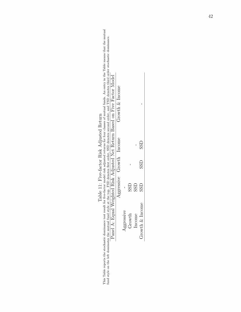
42

Tab

le11

:F

ive-

fact

orR

isk

Adju

sted

Ret

urn

This

Table

rep

ort

sth

est

och

ast

icd

om

inance

test

resu

ltfo

rfi

ve-

fact

or

mod

elri

skad

just

edre

turn

sfo

rfo

ur

class

esof

mu

tual

fun

ds.

An

entr

yin

the

Tab

lem

ean

sth

at

the

mu

tual

fun

dst

yle

on

the

left

dom

inate

sth

em

utu

al

fund

style

at

the

top

.F

SD

den

ote

sfi

rst

ord

er,

SS

Dden

ote

sse

con

dord

er,

an

dT

SD

den

ote

sth

ird

ord

erst

och

ast

icdom

inan

ce.

Pan

elA

:E

qual

Wei

ghte

dR

isk

Adju

sted

Net

Ret

urn

Bas

edon

Fiv

eF

acto

rM

odel

Agg

ress

ive

Gro

wth

Inco

me

Gro

wth

&In

com

eA

ggre

ssiv

e-

Gro

wth

SSD

-In

com

eSSD

-G

row

th&

Inco

me

SSD

SSD

SSD

-

43

Figure 4: CDF for VW Mutual Fund and Market ReturnsThis Figure plots the CDF of the VW mutual fund and market returns. In the first Panel, the solid blue line is the CDF ofmarket returns and the red line is the CDF of VW mutual fund net returns. In the second Panel, the solid blue line is the CDFof market returns and the red line is the CDF of VW mutual fund gross returns. The sample period is from March 1980 andDecember 2015.

−0.25 −0.2 −0.15 −0.1 −0.05 0 0.05 0.1 0.150

0.2

0.4

0.6

0.8

1

Monthly Returns

Pro

babi

lity

Market and VW Mutual Fund Net Return

MarketVW Mutual Fund Net Return

−0.25 −0.2 −0.15 −0.1 −0.05 0 0.05 0.1 0.150

0.2

0.4

0.6

0.8

1

Monthly Returns

Pro

babi

lity

Market and VW Mutual Fund Gross Return

MarketVW Mutual Fund Gross Return

44

Table 12: Stochastic Dominance Test Statistics for VW Mutual Fund and Market ReturnsThis Table shows the stochastic dominance test results between the market and value-weighted mutual fund returns. The sampleincludes all domestic actively managed equity mutual funds in the CRPS-MFLINK merged dataset from March 1980-December2015. Panel A reports the stochastic dominance test results for net returns and Panel B reports the stochastic dominancetest results for the gross return. P-values are based on subsampling,which takes samples without replacement of various blocksizes from the original sample. FSD denotes first order, SSD denotes second order, and TSD denotes third order stochasticdominance.

Test Stat Subsample Block Size10 30 50

Panel A: Market v.s.VW Mutual Fund Net ReturnsAverage Mutual Fund FSD 0.44 (0.00) (0.00) (0.00)vs. Market SSD 0.01 (0.00) (0.00) (0.01)

TSD 0.001 (0.05) (0.05) (0.04)Market FSD 0.31 (0.00) (0.00) (0.00)vs. Average Mutual Fund SSD 0.01 (0.00) (0.00) (0.00)

TSD 0.001 (0.00) (0.01) (0.00)Panel B: Market v.s.VW Mutual Fund Gross ReturnsAverage Mutual Fund FSD 0.37 (0.00) (0.00) (0.00)vs. Market SSD 0.01 (0.00) (0.06) (0.04)

TSD 0.001 (0.02) (0.05) (0.05)Market FSD 0.34 (0.00) (0.00) (0.00)vs. Average Mutual Fund SSD 0.02 (0.00) (0.00) (0.00)

TSD 0.001 (0.00) (0.00) (0.00)

45

Table 13: Stochastic Dominance Test Result for the Market and Four Mutual Fund ClassesThis Table reports the stochastic dominance test results for the returns of the four mutual fund classes and the market. Anentry in the table means that the mutual fund style on the left dominates the mutual fund style/market at the top. FSDdenotes first order, SSD denotes second order, and TSD denotes third order stochastic dominance.

Panel A: VW Net ReturnsAggressive Growth Market Income Growth & Income

Aggressive -Growth TSD -Market SSD -Income TSD TSD TSD -Growth & Income TSD TSD TSD -

Panel B: VW Gross ReturnsAggressive Growth Market Income Growth & Income

Aggressive -Growth TSD -Market TSD -Income TSD TSD TSD -Growth & Income TSD TSD TSD -

46

Table 14: Risk Adjusted Return Performance for Value-weighted Mutual FundsThis Table reports the stochastic dominance test results for four-factor model and five-factor model risk adjusted returns forfour classes of mutual funds. An entry in the table means that the mutual fund style on the left dominates the mutual fundstyle at the top. FSD denotes first order, SSD denotes second order, and TSD denotes third order stochastic dominance.

Panel A: Value Weighted Risk Adjusted Net Return Based on Four-factor ModelAggressive Growth Income Growth & Income

Aggressive -Growth TSD -Income TSD -

Growth & Income TSD SSD SSD -

Panel B: Value Weighted Risk Adjusted Net Return Based on Five-factor ModelsAggressive Growth Income Growth & Income

Aggressive -Growth TSD -Income TSD -

Growth & Income TSD SSD SSD -