Hong Kong Baptist University

Stochastic dominance analysis of Asian hedge fundsWONG, Wing Keung; Phoon, Kok Fai; Lean, Hooi Hooi

Published in:Pacific Basin Finance Journal

DOI:10.1016/j.pacfin.2007.07.001

Published: 01/06/2008

Link to publication

Citation for published version (APA):WONG, W. K., Phoon, K. F., & Lean, H. H. (2008). Stochastic dominance analysis of Asian hedge funds. PacificBasin Finance Journal, 16(3), 204-223. https://doi.org/10.1016/j.pacfin.2007.07.001

General rightsCopyright and intellectual property rights for the publications made accessible in HKBU Scholars are retained by the authors and/or othercopyright owners. In addition to the restrictions prescribed by the Copyright Ordinance of Hong Kong, all users and readers must alsoobserve the following terms of use:

• Users may download and print one copy of any publication from HKBU Scholars for the purpose of private study or research • Users cannot further distribute the material or use it for any profit-making activity or commercial gain • To share publications in HKBU Scholars with others, users are welcome to freely distribute the permanent publication URLs

Downloaded on: 22 Mar, 2022

Stochastic Dominance Analysis of Asian Hedge Funds:

Wing-Keung Wonga

Kok Fai Phoonb

Hooi Hooi Leanc

aDepartment of Economics, Hong Kong Baptist University WLB, Shaw Campus Kowloon Tong Hong Kong Tel: (852) 3411-7542 Fax: (852) 3411-5580 awong@hkbu.edu.hk bDepartment of Accounting and Finance, Monash University P.O. Box 197, Caulfield East, VIC 3145, Australia Tel: 613-9903-2792 Fax: 613-9903-2422 kokfai.phoon@buseco.monash.edu.au cSchool of Social Science, Universiti Sains Malaysia 11800 Minden, Penang, Malaysia. Tel: 604-653-2663 Fax: 604-657-0918 leanmy@gmail.com

1

Stochastic Dominance Analysis of Asian Hedge Funds

ABSTRACT

We employ the stochastic dominance approach that utilizes the entire return distribution

to rank the performance of Asian hedge funds as traditional mean-variance and CAPM

approaches could be inappropriate given the nature of non-normal returns. We find both

first-order and higher-order stochastic dominance relationships amongst the funds and

conclude that investors would be better off by investing in the first-order dominant

funds to maximize their expected wealth. By investing in higher-order dominant funds,

risk-averse investors can maximize their expected utilities but not their wealth. In

addition, we find the common characteristic for most pairs of funds is that one fund is

preferred to another in the negative domain whereas the preference reverses in the

positive domain. We conclude that the stochastic dominance approach is more

appropriate compared with traditional approaches as a filter in hedge fund selection.

Compared with traditional approaches, the SD approach, not only is assumption free,

but also provides greater insights to the performance and risk inherent in a hedge fund’s

track record.

JEL Classification: G11, G15 Key words: hedge funds, stochastic dominance, risk-averse investors, performance measurement.

2

1. INTRODUCTION

There is an increasing trend to include alternative investments in managed

portfolios. An often cited reason is the diversification benefits obtained for doing so.

Hedge funds as an alternative investment have become more popular among

institutional investors. We have also seen financial institutions marketing hedge fund

investments to retail investors. The hedge funds industry has experienced extraordinary

growth over the last decade. Hedge funds that focus on investing in Asia have been

established at an increasing pace. While, 30 new funds were established in 2000 and 20

in 2001, the Bank of Bermuda reported that 66 new hedge funds were started in Asia in

2002 and 90 in 2003. Most of the Asian hedge fund managers are located in Australia,

Singapore, Hong Kong, and Japan, although several manage the Asian funds out of

Europe or the U.S.

According to EurekaHedge, there are more than 520 hedge funds operating in Asia

(including those in Japan and Australia), with assets under management estimated at

more than US$15 billion as of end 2004. Due to its relative small size compared with

the global hedge fund industry (with assets under management in excess of US$1

trillion), we expect strong growth of Asian hedge funds in the near future given the

potential to provide diversification benefits along with strong growth in both the real

and financial sectors in the Asian economies. This potential along with the general lack

of transparency of hedge funds motivates us to understand Asian hedge funds

performance, specifically to provide a methodology that is useful for investors to filter

or rank potential investments based on their past performance. We note that future

returns of hedge funds and their risk profile are not easily predicted using past data and

as Kat and Menexe (2003) suggested, the benefit of a track record lies in the insights it

provides in the performance on one fund’s risk relative to that of another.

3

Section 2 of this paper reviews the literature and motivates the analyses carried out.

The data and methodologies employed are described in Section 3. Empirical results and

their implications are presented in Section 4 and Section 5 concludes.

2. LITERATURE REVIEW AND MOTIVATION

Typically, hedge fund managers adopt investment strategies to provide absolute

returns under different market conditions compared with traditional fund managers who

manage relative to benchmarks. It is commonly believed that hedge funds can generate

positive alphas and the returns provided are generally uncorrelated with the traditional

asset classes. Hedge fund managers use a range of strategies to generate such returns.

Fung and Hsieh (1999a) classified hedge fund strategies as directional (or market

timing) and non-directional. The directional approach dynamically bets on the expected

directions of the markets that fund managers will long or sell-short securities to capture

gains from the advance and decline of their counterpart stocks or indices. In contrast, by

exploiting structural anomalies in the financial market, the non-directional approach

attempts to extract value from a set of embedded arbitrage opportunities within and

across securities.

Comparing the performance of managed funds is not a straightforward task and the

strategies employed by hedge fund managers have introduced new problems. Firstly,

hedge funds including those that invest in Asia have low correlations with the

traditional asset classes like stocks and bonds and attempt to offer protection in falling

and/or volatile markets (Amenc et al., 2003). Hence, comparing hedge funds returns to

standard market indices would be erroneous since hedge funds have an entirely different

objective compared with traditional managed funds (Gregoriou et al., 2005).

Contemporary finance advocates the use of the mean-variance (MV) criterion developed

by Markowitz (1952) for portfolio construction and the capital asset pricing model

(CAPM) statistics developed by Sharpe (1964), Treynor (1965) and Jensen (1969) for

4

managed funds performance evaluation. Many of the studies using such traditional

measures (see, for example, Ackerman et al., 1999; Liang, 1999) conclude that hedge

funds generate superior results.

Over the last decade, extensive empirical analyses had been carried out to

determine the statistical properties of hedge fund returns. The conclusion of these

studies is that hedge fund returns are generally more skewed and leptokurtic than

expected if the underlying distribution is normally distributed. Lavinio (2000) argued

that many hedge funds have distributions with fat-tails, and so normality assumptions

on the distribution of hedge fund returns are generally not correct. Fung and Hsieh

(2000) documented that hedge funds have fat tails resulting in a greater number of

extreme events than one would normally anticipate. Brooks and Kat (2002) found that

hedge fund index returns are not normally distributed. They argued that while hedge

funds may offer relatively high means and low variances, such funds give investors both

third and fourth moments attribute that are exactly the opposite to those that are

desirable.

As the return distributions of hedge funds are generally non-normal, the MV

criterion and the CAPM statistics may not be appropriate to assess the relative

performance of hedge funds. Fung and Hsieh (1997) documented that measures such as

the Sharpe ratio could pose problems due to the option-like returns that hedge funds

generate. Kat (2003) noted that modern portfolio theory is too simplistic to deal with

hedge funds. He maintained that Sharpe ratios and standard alphas could be misleading

in analyzing such investments. This makes the use of traditional performance measures

questionable.

Investors who use volatility as the sole measure of the riskiness of hedge fund

returns could also be misled. While some hedge funds may have low standard deviation,

this does not mean that they are relatively riskless. They may well harbor skewness and

kurtosis, which make them risky. Furthermore, traditional Sharpe ratios usually

5

overestimate fund performance due to negative skewness and leptokurtic returns

(Brooks and Kat, 2002). As a starting point, our study first employs the MV criterion

and CAPM statistics to investigate the performance of Asian hedge funds and some

market indices. One finding is that hedge funds do not dominate the market indices used

or vice versa further motivating the need to explore other alternative approaches to

determine the benefits (if any) of including hedge funds in managed portfolios.

Given that traditional performance measures could provide erroneous results, many

approaches have been offered as alternatives to evaluate hedge fund performance.

Edwards and Caglayan (2001) and Gregoriou et al. (2002) used multifactor models to

examine hedge fund performance. However, as dynamic trading strategies are employed

by hedge funds, exposure to market factors is unlikely to be stable overtime. Multifactor

models possess low predictive power. Furthermore, hedge funds are known as absolute

return vehicles and their aim is to provide superior performance with low volatility in

both bull and bear markets as opposed to comparing their relative performance to

traditional market indices (Brealey and Kaplanis, 2001).

Regardless of the ability of existing and frequently used models to explain hedge

fund returns, the dynamic trading strategies employed along with skewed returns

distribution remains a problem for hedge fund performance evaluation. Some have

proposed the use of longitudinal analyses to better describe temporal features of hedge

fund performance. Brown et al. (2001) applied survival analysis to estimate the

lifetimes of hedge funds and found that these are affected by factors such as their size,

their performance and their redemption period. Getmansky et al. (2004) examined the

illiquidity exposure of hedge funds. Agarwal and Naik (2004) proposed a general asset

class factor model comprising of option-based and buy-and-hold strategies to

benchmark hedge fund performance.

On the other hand, studies have applied the Value-at-Risk (VaR) and conditional-

VaR (CVaR) (see for example, Jorion, 2000; Rockafellar and Uryasev, 2000, 2002;

6

Alexander and Baptista, 2002, 2004) methodology to hedge funds. Lhabitant (2001)

reported factor model-based VaR figures for some hedge funds. Gupta and Liang (2005)

examined the risk characteristics and capital adequacy of hedge funds through the VaR

approach. They showed that VaR-based measures are superior to traditional risk

measures like standard deviation of returns and leverage ratios, in capturing hedge fund

risk. However, Ogryczak and Ruszczynski (2002), Leitner (2005) and Ma and Wong

(2006) noted that stochastic dominance (SD) approach is superior as whatever

information obtained by applying VaR and CVaR could be obtained by the SD

approach.

Recently, Gregoriou et al. (2005)1 applied data envelopment analysis (DEA) to

evaluate the performance of different classes of hedge funds. It is a useful tool for

ranking self appraised and peer group appraised hedge funds. Lee et al. (2006)

introduced a practical non-linear approach based on first and cross-moments analyses in

up and down markets to assess the risk and performance of Asian hedge funds. They

found that while all funds provide diversification in the sense that they are not perfectly

correlated with market index returns, few funds provide downside protection along with

upside capture that is assumed to be preferred by investors. They found that funds

having these preferred attributes provided returns that are not, on average, significantly

less than those that do not provide such preferred attributes. The same data sample was

used in our paper. We have found that selected funds provide both stochastic

dominating returns as well as funds that provide upside capture and downside protection,

as well as stability in volatile condition at insignificant cost.

The search for performance measures for hedge funds is an on-going process. We

recommend the SD approach that allows investors to appropriately rank fund

performance without the need for strong assumptions on investors’ utility function or

the return distribution of asset returns. SD rules offer superior criteria on which to base

1 Gregoriou et al., (2005) provided a detailed literature review of hedge fund performance measures.

7

investment decisions compared with the traditional MV and CAPM analysis because the

assumptions underlying SD are less restrictive. Taylor and Yoder (1999) argued that SD

incorporates information on the entire distribution, rather than the first two moments

and requires no precise assessment as to the specific form of investors’ risk preference

or utility function.

The SD approach had been used in the evaluation of performance of mutual funds

since the 1970s (Levy and Sarnat, 1970; Porter, 1973). Recently, Taylor and Yoder

(1999) used the SD approach to compare the performance between load and no-load

funds during the 1987 crash. Kjetsaa and Kieff (2003) documented that the SD

approach provides a collateral and feasible strategy to reveal relative investment

preferences by discriminating among and parsing the universe of mutual fund

opportunities. More recently, Gasbarro et al. (2007) utilized both the SD approach and

the CAPM criterion to compare the performance of 18 country market indices (iShares)

and found that SD appears to be both more robust and discriminating than the CAPM in

the ranking of iShares.

In this paper, we use the Davidson and Duclos (DD, 2000) or DD test to determine

if the difference in the cumulative density functions of the returns of two hedge funds

are statistically significant. The SD tests developed by Barrett and Donald (BD, 2003)

and Linton et al. (LMW, 2005) are computed for comparison.

We use the DD test to determine if SD occurred among the 70 individual Asian

hedge funds during our sample period. We find that over the sample period (January

2000 to December 2004), some hedge funds dominate others. Conversely, some funds

do not dominate any other hedge funds, but they themselves are not dominated by other

hedge funds as well. Surprisingly, for the two equity market indices being examined,

viz. MSAUCPI (Morgan Stanley Pacific Index) and S&P 500 are dominated by 21 and

15 other indices/funds respectively at the first-order. In addition, we find the common

characteristic for most pairs of funds is that one fund is preferred to another in the

8

negative domain or bear markets whereas the preference reverses in the positive domain

or bull runs.2 Our suggested methodology can be a useful filter for fund selection for

different levels of risk aversion among investors to maximize their expected wealth

and/or utilities along with the usually skewed and non-normal characteristics of hedge

fund returns.

3. DATA AND METHODOLOGY

The data analyzed in this study are the monthly returns of the 70 Asian hedge funds

reported by the EurekaHedge database for the sample period from January 2000 to

December 2004. For completeness, we include the EurekaHedge Asia Ex-Japan (IX1),

Eureka Hedge Japan (IX2) and EurekaHedge Asian Hedge Fund (IX3) indices. We also

carry out our analysis on two traditional equity market indices, viz. the Morgan Stanley

Pacific Index (MSAUCPI)3 (IX4) and the S&P500 index (IX5). We include the S&P

500 in our study as traditional U.S. based fund managers and investors may use the S&P

500 as the equity benchmark. If they are investing internationally, diversification

benefits can be measured relative to a regional benchmark constructed by Morgan

Stanley, like the MSAUCPI. The 3-month U.S. T-bill rate and the Morgan Stanley

Capital International Global index (MSCI) proxy the risk-free rate and the global market

index respectively are used for CAPM statistics.

2 Post and Levy (2005) studied the dominance of assets in the negative and positive domains and

concluded that investors are risk-averse in bear markets and risk-seeking in bull markets. We agree with

Post and Levy that investors could make inference in bear (bull) markets when examining negative

(positive) domain though bear (bull) markets are not exactly equal to negative (positive) domain of the

returns. 3 The MSAUCPI is a free-float-adjusted market capitalization index that is designed to measure the equity

market performance in the Australasian region. It includes 12 emerging and developed market countries:

viz. Australia, China, Hong Kong, Indonesia, Japan, Korea, Malaysia, New Zealand, Philippines,

Singapore, Taiwan and Thailand.

9

The MV criterion and CAPM statistics are commonly used for mutual funds

performance evaluation. The MV criterion (Markowitz, 1952; Tobin, 1958) states that,

for the returns of any two funds Y and Z with means y and z and standard

deviations, y and z respectively, Y is said to dominate Z if y z and y z .4

The CAPM risk-adjusted performance measures developed by Sharpe (1964), Treynor

(1965) and Jensen (1969) are the Sharpe ratio, Treynor’s index and Jensen (alpha)

index.5 However, both the MV criterion and CAPM measures are derived assuming the

Von Neumann-Morgenstern (1944) quadratic utility function and that returns are

normally distributed (Feldstein, 1969; Hanoch and Levy, 1969). Thus, the reliability of

performance comparisons using the MV criterion and CAPM analysis depends on the

degree of non-normality of the returns data and the nature of the (non-quadratic) utility

functions (Fung and Hsieh, 1999b).

Essentially, the most commonly-used SD rules that correspond with three broadly

defined utility functions are first-, second- and third-order SD for risk averters, denoted

by FSD, SSD and TSD respectively. Formally, we let F and G be the cumulative

distribution functions (CDFs) and f and g are the corresponding probability density

functions (PDFs) of the returns for two funds Y and Z respectively with common

support of [a, b] (a < b). Define

0H h and 1

x

j jaH x H t dt for h = f, g , ,H F G and 1, 2,3j .6 (1)

Fund Y would dominate Fund Z by FSD if and only if 1 1F x G x ; by SSD if and

only if 2 2F x G x ; and finally, by TSD if and only if 3 3F x G x for all x, and

4 Refer to Meyer (1987), Wong (2007) and Wong and Ma (2007) on the relation between stochastic

dominance and mean-variance rules. 5 Readers may refer to Sharpe (1964), Treynor (1965) and Jensen (1969) for the details and discussions of

these statistics. 6 Refer to Wong and Li (1999), Anderson (2004) and Wong and Chan (2007) for the discussions on the

definitions.

10

the strict inequality holds for at least one value of x ; and Y has higher expected return

than Z.

The existence of FSD (SSD, TSD) implies that the expected wealth (utilities) of

investors are always higher when holding the dominant fund than holding the

dominated fund and, consequently, the dominated fund should not be chosen. Investors

exhibit non-satiation (more is preferred to less) under FSD; non-satiation and risk

aversion under SSD; and non-satiation, risk aversion, and decreasing absolute risk

aversion (DARA) under TSD. We note that hierarchical relationship exists in SD (Levy

1992, 1998): FSD implies SSD, which in turn implies TSD. However, the converse is

not true. Thus, only the lowest dominance order of SD is reported in practice.

Recent advances in SD empirical techniques allow the statistical significance of SD

to be determined. To date, the SD tests for risk averters have been well developed, for

example, see McFadden (1989), Klecan et al. (1991), Kaur et al. (1994), Anderson

(1996, 2004), Davidson and Duclos (DD, 2000), Barrett and Donald (BD, 2003) and

Linton et al. (LMW, 2005). The DD test has been found to be one of the most powerful,

but yet less conservative in size (Wei and Zhang, 2003; Tse and Zhang, 2004 and Lean

et al., 2007); while the BD test is another powerful test instrument and the LMW is

useful as it is extended from Kolmogorov-Smirnov test for FSD and SSD by relaxing

the iid assumption. We report the results of the DD test and skip reporting those of BD

and LMW tests as the former is the only SD statistics that test the SD relationship up to

the third-order and the results of both BD and LMW tests are consistent with those of

the DD test.

For any two funds Y and Z with CDFs F and G respectively and for a grid of pre-

selected points x1, x2… xk, the order-j DD test statistics, ( )jT x (j = 1, 2 and 3), is:

11

ˆˆ ( ) ( )( )

ˆ ( )

j jj

j

F x G xT x

V x

, (2)

where ,ˆ ˆ ˆ ˆ( ) ( ) ( ) 2 ( ),j j j

j Y Z Y ZV x V x V x V x

1

1

1ˆ ( ) ( ) ,( 1)!

Nj

j ii

H x x hN j

2( 1) 22

1

11, 2

1

1 1ˆ ˆ( ) ( ) ( ) , , ; , ;(( 1)!)

1 1 ˆˆ ˆ( ) ( ) ( ) ( ) ;(( 1)!)

Nj j

H i ji

Njj j

Y Z i i j ji

V x x h H x H F G h y zN N j

V x x y x z F x G xN N j

in which jF and jG are defined in (1).

It is empirically impossible to test the null hypothesis for the full support of the

distributions. Thus, Bishop et al. (1992) proposed to test the null hypothesis for a pre-

designed finite number of x. Specifically, the following hypotheses are tested:

0

1

2

: ( ) ( ) , for all , 1, 2,..., ;

: ( ) ( ) for some ;

: for all , for some ;

: for all , for some .

j i j i i

A j i j i i

A j i j i i j i j i i

A j i j i i j i j i i

H F x G x x i k

H F x G x x

H F x G x x F x G x x

H F x G x x F x G x x

We note that in the above hypotheses, AH is set to be exclusive of both 1AH

and 2AH , which means that if either 1AH or 2AH is accepted, we will not say AH is

accepted. Under the null hypothesis, DD showed that jT x is asymptotically

distributed as the Studentized Maximum Modulus (SMM) distribution (Richmond,

1982) to account for joint test size. To implement the DD test, the test statistic at each

grid point is computed and the null hypothesis, 0H , is rejected if the test statistic is

significant at any grid point. The SMM distribution with k and infinite degrees of

freedom, denoted by kM , , is used to control for the probability of rejecting the overall

null hypotheses. The following decision rules are adopted based on 1- percentile of

kM , tabulated by Stoline and Ury (1979):

12

, 0

, , 1

, , 2

,

If ( ) for 1,..., , accept ;

if ( ) for all and ( ) for some , accept ;

if ( ) for all and ( ) for some , accept ; and

if ( ) for s

kj i

k kj i j i A

k kj i j i A

kj i

T x M i k H

T x M i T x M i H

T x M i T x M i H

T x M

,ome and ( ) for some , accept .kj i Ai T x M i H

Accepting either H0 or HA implies non-existence of any SD relationship, non-

existence of any arbitrage opportunity between these two hedge funds and neither of

these two hedge funds are preferred to one another. However, if 1AH or 2AH of order

one is accepted, a particular hedge fund stochastically dominates another hedge fund at

first-order. In this situation, any non-satiated investor will increase her/his expected

wealth if s/he switches from the dominated hedge fund to the dominant one. 7 On the

other hand, if 1AH or 2AH is accepted for order two or three, a particular hedge fund

stochastically dominates the other at second- or third-order. In this situation, arbitrage

opportunity does not exist and switching from one hedge fund to another will only

increase investors’ expected utilities, but not expected wealth.

The DD test compares the distributions at a finite number of grid points. Various

studies examine the choice of grid points. For example, Tse and Zhang (2004) showed

that an appropriate choice of k for reasonably large samples ranges from 6 to 15. Too

few grids will miss information of the distributions between any two consecutive grids

(Barrett and Donald, 2003) and too many grids will violate the independence

assumption required by the SMM distribution (Richmond, 1982). To make more

detailed comparisons without violating the independence assumption, we follow Fong et

al. (2005) and Gasbarro et al. (2007) to make 10 major partitions with 10 minor

partitions within any two consecutive major partitions in each comparison and to make

the statistical inference based on the SMM distribution for k=10 and infinite degrees of

7 Refer to our conclusion for the discussions.

13

freedom8. This allows the examination of the consistency of both magnitudes and signs

of the DD statistics between any two consecutive major partitions without violating the

independent assumption.

4. EMPIRICAL FINDINGS AND IMPLICATIONS

4.1 MV Criterion and CAPM Statistics Results

We begin our empirical analysis of the Asian hedge funds using the MV criterion.

The means and the standard deviations of the returns for all 70 Asian hedge funds

studied are plotted and shown in Figure 1. The figure reveals that in general the means

and standard deviations move together and thus the results are consistent with modern

portfolio theory that higher mean accompanies higher risk. We depict in Figure 2 the

risks versus returns trade-off and the corresponding efficient frontier for the 70 funds.

We find that most of the funds are not in the efficient frontier. We exhibit in Table 1 the

summary statistics of the five indices (IX1 to IX5) and the four ‘most outstanding

funds’ (AHF01, AHF18, AHF39 and AHF47) with largest or smallest means, standard

deviations or Sharpe ratios.9 Interestingly, we find that the most outstanding funds

reported in Table 1 adopt different investment strategies: AHF01 is Distressed Debt,

AHF18 is Long/Short Equities, AHF39 is Multi-Strategy and AHF47 is Macro. 10 From

Table 1, the average monthly mean return of the 70 Asian hedge funds is observed to be

8 Refer to Lean et al (2007) for the reasons. Critical values are: 3.691, 3.254 and 3.043 for 1%, 5% and

10% level of significance tabulated in Stoline and Ury (1979). 9 Refer to Table 1 for the full names of IX1-IX5, AHF01, AHF18, AHF39 and AHF47 and the

characteristics of the funds. 10 Macro Strategy: A Macro fund aims to profit from changes in global economies, typically brought

about by shifts in government policy that impact interest rates, in turn affecting currency, stock, and bond

markets; Participates in all major markets - equities, bonds, currencies and commodities - though not

always at the same time. Uses leverage and derivatives to accentuate the impact of market moves. Utilizes

hedging, but the leveraged directional investments tend to make the largest impact on performance.

(http://www.magnum.com/hedgefunds/abouthedgefunds.asp).

14

higher than the monthly mean returns of the market indices except AA EH Asia ex

Japan Index whereas the average standard deviation of monthly returns of the 70 Asian

hedge funds is larger than the standard deviations of the market indices except

MSAUCPI, inferring that hedge funds, in general, produce higher return but generate

higher risk.

The means and standard deviations vary widely across Asian hedge funds. For

example, AHF47 possesses the largest monthly mean return (0.03648) and the largest

standard deviation (0.1941) among the 70 hedge funds and the five market indices while

both AHF18 and AHF39 exhibit the lowest monthly mean returns (-0.0069) and

smallest standard deviation (0.00787) respectively. Interestingly, using the MV criterion,

we have found a fund, AHF47, possessing the largest mean that does not dominate any

other fund, including AHF18 and AHF39. Thus, we conclude that, using the MV

criterion, a fund with the largest mean return may not be a good investment choice. On

the other hand, AHF01 and AHF39 are found to have significant higher means and

smaller standard deviations (not significant) than AHF18. Therefore, both AHF01 and

AHF39 dominate AHF18 by the MV criterion.

------------------------------------------------- Insert Tables 1 and 2, Figures 1 and 2 here -------------------------------------------------

Next, we investigate the CAPM measures for all indices and funds.11 From

Table 1, AHF01 exhibits the largest Sharpe ratio (0.83995) while AHF18 has the lowest

(-0.2948). Furthermore, AHF39 possesses the highest Treynor (0.7199) while AHF47

obtains the highest Jensen (0.0369) measures. A summary of dominance results among

the 4 most outstanding Asian hedge funds and the 5 indices measured by the MV

criterion and all the CAPM statistics are presented in Table 2.12 From the table, we find

that sometimes a fund dominates another fund by a CAPM statistic but the dominance

relation can be reverse if measured by other CAPM statistic(s). For example, AHF39

dominates AHF01 by Treynor index whereas AHF01 dominates AHF39 by both Sharpe 11 We only report the most important results in Table 1. Other results are available upon request. 12 Refer to the note in Table 2 on how to read the table.

15

ratio and Jensen index. Thus, we conclude that, in general, different funds are chosen

using different CAPM measures. In addition, our results show that some of the return

distributions are non-normal and exhibit both negative skewness and excess kurtosis.

Specifically, 19 skewness, 26 kurtosis and 27 Jarque-Bera measures are significant at

the 0.05 level,13 highlighting the non-normality feature for the returns of these hedge

funds. As noted by Kat (2003) and Kooli et al. (2005), the modern portfolio theory is

too simplistic to deal with hedge funds. Furthermore, Gregoriou et al. (2005) pointed

out that CAPM measures will usually overestimate and miscalculate hedge funds

performance. Therefore, the results drawn by both the MV and CAPM statistics can be

misleading.

Nonetheless, from our analysis using the MV criterion and CAPM statistics, we

observe some consistent outcomes. We find, for example, that both AHF01 (fund with

the largest Sharpe ratio) and AHF39 (fund with the smallest standard deviation)

dominate AHF18 (the fund with the smallest Sharpe ratio) across most of the MV and

CAPM statistics. Thus, one may ask whether the fund with the largest Sharpe ratio and

the fund with the smallest standard deviation are the best choices while the fund with

the smallest Sharpe ratio is the worst choice. To explore this question and to examine

alternative measures to choose funds, we utilize the SD approach.

4.2 Stochastic Dominance Results

DD stated that the null hypothesis of equal distribution could be rejected if any

value of the test statistic, jT (j=1,2,3; see eqn (2)), is significant. In order to minimize

the Type II error and to accommodate the effect of almost SD (Leshno and Levy, 2002),

we follow Gasbarro et al. (2007) to use a conservative 5% cut-off point for the

proportion of test statistics in statistical inference. Using a 5% cut-off point, we

conclude fund Y dominates fund Z if we find at least 5% of jT to be significantly

13 The results are partially displayed in Table 1. Detailed results are available upon request.

16

negative and no portion of jT is significantly positive. The reverse holds if the fund Z

dominates fund Y.

------------------------------- Insert Tables 3 and 4 here -------------------------------

We depict in Table 3 the DD test statistics for the pair-wise comparison of the 5

market indices and the 4 most outstanding Asian hedge funds and display in Table 4 the

summary of their DD dominance results. From the tables14, we first find that in general

one could not conclude that funds will always outperform indices and vice versa

because there exist FSD relationships from funds to indices as well as from indices to

funds. In addition, we conclude that risk averters may not always prefer investing in

funds than indices and vice versa because there exist SSD relationships from funds to

indices as well as from indices to funds.

Secondly, we find that in our sample period AA EH Japan Index is the most

favorable index and MSAUCPI is the least favorable index as the former dominates 11

(23) other indices/funds at first (second) order but is dominated only by AHF01 at SSD

whereas the latter is dominated by 21 (19) indices/funds at first (second) order but

dominates only 2 indices/funds at second order. On the other hand, AHF01 is the most

favorable fund as it dominates 16 (38) other indices/funds at first (second) order and is

not dominated by any other index/fund. Similarly, from the tables, one could conclude

that AHF39 is the second most favorable fund. The two least favorable funds are

AHF47 and AHF18. The former is dominated by 63 indices/funds at second order but

does not dominate any index/fund while the latter is dominated by 17 (4) indices/funds

at first (second) order and dominates two other indices/funds. Between AHF47 and

AHF18, though the former is dominated by more indices/funds, AHF18 is the least

favorable as it gets the largest number of indices/funds dominating it at first order, this

14 One may refer to the notes in the tables on how to read the tables.

17

means that investors will increase their expected wealth by selling AHF18 and longing

any fund, say for example, AHF01, dominating it. However, when selling AHF47 and

buying any fund dominating it could only increase one’s expected utility, not expected

wealth. Thus, we conclude that AHF18 is the least favorable one.

Now, we come back to our conclusion drawn using the MV criterion and CAPM

statistics where we find that AHF01 and AHF39 are the most favorable funds while

AHF18 is the least favorable fund. Using the SD approach, we demonstrate that AHF01

(AHF39) is the (second) most favorable fund whereas AHF18 (AHF47) is the (second)

least favorable fund. This finding leads us to conjecture that the SD approach could

exploit more information to decide on fund choice than its MV and CAPM counterparts.

Based on this conjecture, we further investigate whether we can acquire additional

information by adopting the SD approach to obtain the percentage of significant DD

statistics for pairs of these funds in details, namely, AHF47 (largest mean) versus

AHF18 (smallest mean), AHF39 (smallest standard deviation) versus AHF47 (largest

standard deviation), AHF01 (largest Sharpe ratio) versus AHF18 (smallest Sharpe ratio),

AHF01 (the most favorable fund under SD) versus AHF39 (the second most favorable

fund under SD). In addition, we include the comparisons of AHF01-AHF47 and

AHF39-AHF18 in our study because these comparisons exhibit FSD relations that

seldom occur empirically. The results are reported in Table 5. We note that our paper is

the first paper to systematically and empirically study first order stochastic domination

in the literature.

---------------------------------------

Insert Table 5 here ---------------------------------------

In Table 5, we apply equation (2) with the preferable fund being the first variable

(F) and the less preferable fund being the second variable (G) in the equation. If the

results behave as expected, there will exist ( 1, 2,3)j j such that there will not be any

significantly positive jT but there will exist some significantly negative jT . For

18

example, as investors are risk-averse, we expect the fund with the smallest standard

deviation (AHF39) will be preferred to the fund with the largest standard deviation

(AHF47). Thus, we place AHF39 as the first variable and AHF47 as the second variable

in equation (2). The DD results displayed in Table 2 show that there are 22(11)

percentage of 1T to be significantly positive (negative), indicating that AHF39 and

AHF47 do not dominate each other at first order. However, we find that all values of

2 3( )T T are non-positive with 15(19) percentage of them to be significantly negative,

implying AHF39 dominates AHF47 at second (third) order SD as expected.

--------------------------------------- Insert Figure 3 here

---------------------------------------

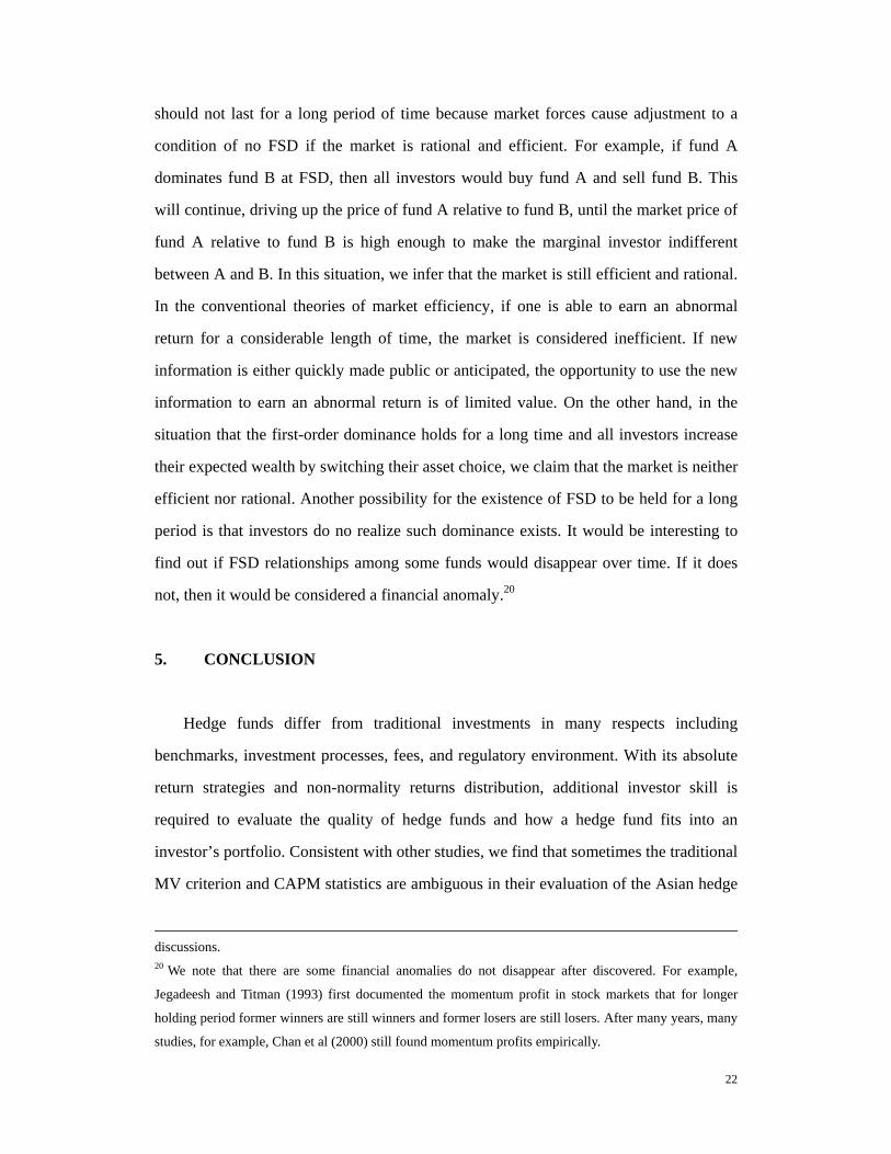
So far, all comparisons behave as expected except the pair AHF47-AHF18. As

AHF47 possesses the highest mean while AHF18 attains the smallest mean and it is a

common sense that all non-satiated investors prefer more to less, we expect AHF47 to

be preferred to AHF18. However, their DD results shown in Table 5 reveal that all

2 3( )T T are non-negative with 11(9) percentage of 2 3( )T T to be significantly positive,

implying that, contradict to the common belief, the fund, AHF18, with the smallest

mean dominates the fund, AHF47, with the largest mean at second (third) order SD.

Hence, we confirm that risk averters and risk-averse investors with DARA who make

portfolio choice on the basis of expected-utility maximization will unambiguously

prefer AHF18 to AHF47 to maximize their expected utilities.

We recall that the MV and CAPM criteria show that AHF18 does not dominate

AHF47 whereas AHF47 dominates AHF18 by Sharpe Ratio, Jensen index and Treynor

index. As AHF47 possesses an insignificantly larger mean but significantly larger

standard deviation than AHF18, one should not be surprised that our SD results reveal

that AHF18 dominates AHF47 at second and third order. This result is consistent with

Markowitz (1991) that investors, especially risk-averse investors, worry more about

downside risk than upside profit. In addition, together with Figure 3, the results from

19

Table 5 show that 9% of 1T is significantly positive in the negative domain whereas

22% of 1T is significantly negative in the positive domain. All these SD information

implies that actually AHF47 and AHF18 do not outperform each other. AHF18 is

preferable in the negative domain whereas AHF47 is preferable in the positive domain

and, overall, risk averters prefer to invest in AHF18 than AHF47. All these information

revealed by utilizing SD could not be obtained by adopting the MV or CAPM

counterparts.

We note that most of the SD comparisons for assets in the literature behave as in

the above comparison: one asset dominates another asset at SSD or TSD (see for

example, Seyhun, 1993). Applying the DD technique, we could obtain more

information than the usual SD comparison as we state in the above example: one asset

dominates another asset on the downside while the reverse dominance relationship can

be found on the upside. This finding is in line with the direction of research in Post and

Levy (2005) who investigate the behaviors of investors in bull and bear markets..

4.3 FSD Results and Discussions

We next explore the FSD relationship in our empirical findings. We find three FSD

relationships: AHF01-AHF18, AHF01-AHF39 and AHF39-AHF18. For illustration, we

only discuss AHF01-AHF18 and AHF01-AHF39 in details. 15 The first pair is

interesting as we compare the fund with the largest Sharpe ratio (AHF01) versus the

fund with the smallest Sharpe ratio. The second is also interesting as AHF01 is the most

preferable fund and AHF39 is the second most preferable fund under SD in our study

and thus one may be surprised that the former first-order stochastically dominates the

latter.

---------------------------------------

15 We skip the discussion of AHF39-AHF18 as it is similar to that of AHF01-AHF18.

20

Insert Figures 4 and 5 here ---------------------------------------

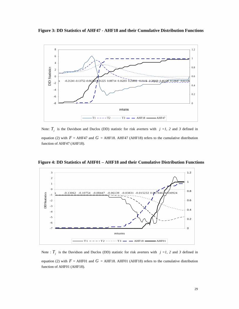
Table 5 shows that, for AHF01-AHF18, none of 1T is significantly positive with

21% of it to be significantly negative. Similarly, the table displays that for AHF01-

AHF39, none of 1T is significantly positive with 27% of it to be significantly negative.

These results imply that AHF01 stochastically dominates both AHF18 and AHF39 at

first order and thus investors will increase their expected wealth if they shift their

investment from AHF18 and/or AHF39 to AHF01.

Recently, using the same dataset, Lee et al. (2006) found that some of the Asian

hedge funds provide upside capture, downside protection, low volatility in down

markets and high volatility in up-markets. Our findings, when comparing the CDF of

AHF01 with that of AHF18 or AHF39, first support the findings of Lee et al. that

AHF01 possesses lower volatility in down markets (and thus provides downside

protection)16 and possesses high volatility in up-markets (and thus provides upside

capture)17. In addition to standard information (such as non-satiated investors will attain

higher expected wealth by investing in AHF01) obtained by the SD approach. Using

SD, we can provide additional to investors. For example, it is shown in Figure 5, that

AHF01 possesses higher volatility on return from 0.02 to 0.04 whereas AHF39 has zero

probability to obtain return greater 0.02. Thus, we claim that SD approach is more

informative than the approach used by Lee et al.

Many studies, for example, Jarrow (1986) and Falk and Levy (1989) claim that

if FSD exists, under certain conditions arbitrage opportunity exist and investors will

16 It is because CDF of AHF01 lies below that of AHF18 and AHF39 statistically in the negative domain

and thus AHF01 possesses smaller probability on the downside. 17 It is because probability on the upside is equal to one minus probability on the downside and because

CDF of AHF01 lies below that of AHF18 and AHF39 statistically. One may draw PDFs of these funds to

reveal a clear picture for the issue.

21

increase their wealth and expected utilities if they shift from holding the dominated

hedge fund to the dominant one. In this paper, we claim that if FSD exists statistically,

arbitrage opportunity may not exist but investors could increase their expected wealth as

well as their expected utilities if they shift from holding the dominated hedge fund to

the dominant one. We explain our claim by these examples. Refer to Figure 4 (5), the

two CDFs do cross and thus the CDF of the dominant fund does not totally lie below

that of the dominated one. Thus, the values of 1T are not totally non-positive in both

figures: there is a positive portion of 1T in the positive (negative) domain in Figure 4

(5), though these positive values are not significant. This shows that AHF18 (AHF39)

does dominate AHF01 in this small portion of the positive (negative) domain or in a

small part of bull run (bear market) though this domination is not statistically

significant. In other words, AHF01 dominates both AHF18 and AHF39 statistically but

not mathematically. Hence, arbitrage opportunity may not exist but investors can still

increase their expected wealth as well as their expected utilities but not their wealth if

they shift their investment from AHF18 and/or AHF39 to AHF01. In addition, even if

one fund dominates another fund at first order mathematically, we claim that arbitrage

opportunity may not exist also as arbitrage opportunity in FSD exists only if the market

is ‘complete’. If the market is not ‘complete’, even FSD exists, investors may not be

able to exploit any arbitrage opportunity there.18

In addition, if the test detect the first-order dominance of a particular fund over

another but the dominance does not last for a long period, these results cannot be used

to reject market efficiency or market rationality.19 In general, the first-order dominance

18 See Jarrow (1986), Falk and Levy (1989) and Wong and Chan (2007) for more discussions. For

example, Jarrow (1986) discovered the existence of the arbitrage opportunities by SD rules. He defined a

‘complete’ market as ‘an economy where all contingent claims on the primary assets trade.’ His Arbitrage

versus SD theorem says that when the market is complete, X stochastically dominates Y in the sense of

FSD if and only if there is an arbitrage opportunity between X and Y. 19 See Falk and Levy (1989), Bernard and Seyhun (1997) and Larsen and Resnick (1999) for more

22

should not last for a long period of time because market forces cause adjustment to a

condition of no FSD if the market is rational and efficient. For example, if fund A

dominates fund B at FSD, then all investors would buy fund A and sell fund B. This

will continue, driving up the price of fund A relative to fund B, until the market price of

fund A relative to fund B is high enough to make the marginal investor indifferent

between A and B. In this situation, we infer that the market is still efficient and rational.

In the conventional theories of market efficiency, if one is able to earn an abnormal

return for a considerable length of time, the market is considered inefficient. If new

information is either quickly made public or anticipated, the opportunity to use the new

information to earn an abnormal return is of limited value. On the other hand, in the

situation that the first-order dominance holds for a long time and all investors increase

their expected wealth by switching their asset choice, we claim that the market is neither

efficient nor rational. Another possibility for the existence of FSD to be held for a long

period is that investors do no realize such dominance exists. It would be interesting to

find out if FSD relationships among some funds would disappear over time. If it does

not, then it would be considered a financial anomaly.20

5. CONCLUSION

Hedge funds differ from traditional investments in many respects including

benchmarks, investment processes, fees, and regulatory environment. With its absolute

return strategies and non-normality returns distribution, additional investor skill is

required to evaluate the quality of hedge funds and how a hedge fund fits into an

investor’s portfolio. Consistent with other studies, we find that sometimes the traditional

MV criterion and CAPM statistics are ambiguous in their evaluation of the Asian hedge

discussions. 20 We note that there are some financial anomalies do not disappear after discovered. For example,

Jegadeesh and Titman (1993) first documented the momentum profit in stock markets that for longer

holding period former winners are still winners and former losers are still losers. After many years, many

studies, for example, Chan et al (2000) still found momentum profits empirically.

23

funds some of the time. At other times, though some of MV and CAPM measures can

identify the dominant funds, they fail to provide detailed information of the dominance

relationship nor on the preferences of investors.

This paper introduces a powerful SD test to present a more complete picture for

hedge fund performance appraisal and to draw inference on the preference of investors

on the funds. The SD approach that is basically free of assumption is used to investigate

the characteristics of the entire distribution of returns and test whether rational investors

benefit from any hedge fund to maximize their expected utilities and/or expected wealth.

An advantage of this approach is that it alleviates the problems that can arise if hedge

fund returns are non-normally distributed. Our approach also allows for a meaningful

economic interpretation of the results. Based on a sample of the 70 individual Asian

hedge funds from the EurekaHedge database, we find the existence of first-order SD

relationship among some hedge funds in the entire sample period; suggesting that all

non-satiated investors could increase their expected wealth as well as their expected

utilities by investing in the Asian hedge funds to explore these opportunities by shifting

their investments from the dominated funds to the dominant funds. We also find the

existence of second-order SD relationship among other funds/indices; indicating that the

non-satiated and risk-averse investors would maximize their expected utilities, but not

their expected wealth by switching from the SSD dominated hedge funds to their

corresponding SSD dominant ones. In addition, by applying the DD technique, we also

discover that in most SD relationships, one fund dominates another fund in the negative

domain while the reverse dominance relationship can be found in the positive domain.

Beside, the normality assumption in the traditional measures, the difference may also

come from the traditional measures definition of an abnormal return as an excess return

adjusted to some risk measures, while the SD tests employ the whole distribution of

returns. The SD measure is an alternative that is superior to the traditional measures to

help investors and fund managers in managing their investment portfolios.

We note that while some hedge funds are dominated by others, other issues may

need to be considered before implementing the SD methodology in the selection of

hedge funds. One issue is that Asian hedge funds may have different redemption timing,

ranging from daily to once a year in rare cases. Hence, investors may prefer funds with

high redemption frequency. We also note that while AHF01 dominates AHF47,

24

investors can only redeem AHF01 quarterly, while the redemption timing for AFH47 is

once a month. Secondly, entry and exit into hedge funds can be costly. These include

search and assessment costs considerable due diligence is often advised for hedge fund

investors. Further, a “hidden” transaction cost may arise in the way hedge fund

managers are rewarded using a performance related fee. Lee et al. (2004) showed that

this fee structure can penalize investors who transact frequently due to the free-rider and

claw-back problems.

Some authors propose using higher order (higher than three) SD in empirical

application. For example, Vinod (2004) recommended employing fourth order SD to

choose investment prospects amongst 1281 mutual funds. We, however, would like to

note that the first three orders are the most commonly-used orders in empirical work on

SD, regardless whether the analyses are simple or complicated. We would also like to

note that a hierarchy exists in SD relationships whereby findings of the first-order SD

implies the second-order SD which in turn implies the third-order SD and the fourth

order SD and so on (Levy 1992, 1998). We thus stopped at third order in this paper. In

addition, we note that Post and Versijp (2007) have developed a new SD test for

multiple comparisons. The advantage of this approach is that they could make multiple

SD comparisons while we ranked the funds pair-wise. As we explore pair-wise

comparison in the domination, we do not apply their test in this study.

Lastly, we find results that are consistent with Kat (2003), Kooli et al. (2005),

Gregoriou et al. (2005) and many others who claim that if the normality assumption

fails, the results drawn using the MV criterion and CAPM statistics can be misleading.

We point out that unlike the SD approach that is consistent with utility maximisation the

dominance findings using the MV and CAPM measures may only be consistent with

utility maximization, if the assets returns are not normally distributed, under very

specific conditions. For example, Meyer (1987), Wong (2007) and Wong and Ma

(2007) show that that if the returns of two assets follow the same location-scale family,

then a MV domination could infer preferences by risk averters on the dominant fund to

the dominated one. Furthermore, if all the regularity conditions are satisfied (for

example, assets follow normality assumption), the MV and CAPM measures be

consistent if asset returns possess second order SD preference characteristic. However,

even if all the regularity conditions are satisfied, the MV and CAPM measures cannot

25

identify the situations in which one fund dominates another one at first or third order SD.

Thus, the SD approach allows better assessments for assets, regardless whether whose

returns are normally or non-normally distributed.

We conclude that the stochastic dominance approach is more appropriate as a filter in

the hedge fund selection process. Compared with the traditional approaches, the SD

approach is more informative, providing greater insights and hence, allowing for better

comparison in the performance and risk inherent in a hedge fund’s track record relative

to that of another.

26

Table 1: Summary Statistics of the Asian Hedge Funds and the Five Market Indices

Mean Std Dev Sharpe Ratio Skewness Kurtosis JB

AA EH Asia ex Japan Index (IX1) 0.01074 0.02474 0.3446 -0.1268 -0.6269 1.1437 AA EH Japan Index (IX2) 0.00779 0.01753 0.3179 0.8404* 1.2776 11.1446** AA EH Index (IX3) 0.00839 0.01692 0.3647 -0.1265 -0.5447 0.9019 MSAUCPI (IX4) -0.00259 0.04950 -0.0970 -0.0782 -1.0969 3.0693 S&P 500 (IX5) -0.00211 0.04708 -0.0917 -0.1031 -0.2931 0.3213 Average (Hedge Funds) 0.00913 0.04784 0.1830 0.2232 1.9470** 41.3997**

Maximum (Hedge Funds) 0.03648 0.19413 0.8399 3.0663** 16.4066** 766.96**

Minimum (Hedge Funds) -0.00690 0.00787 -0.2948 -1.6243** -1.0969 0.0718

AHF01 (ADM Galleus Fund) 0.01267 0.01245 0.8399 -0.1083 -0.4376 0.5961 AHF18 (Furinkazan Fund USD) -0.00690 0.03092 -0.2948 -1.5567** 7.8761** 179.32**

AHF39 (LIM Asia Arbitrage Fund) 0.00601 0.00787 0.4824 -0.4813 0.1959 2.4124

AHF47 (Pacific-Asset Alpha Fund) 0.03648 0.19413 0.1765 1.2334** 1.2206 18.9381**

Note: AHF01, AHF18, AHF39 and AHF47 are the ‘most outstanding funds’ in which AHF47 possesses the

largest monthly mean return (0.03648) and the largest standard deviation (0.1941); AHF18 exhibits the

lowest monthly mean return and the smallest Sharpe ratio (-0.2948); AHF39 exhibits the smallest standard

deviation (0.00787); AHF01 exhibits the largest Sharpe ratio (0.83995); AHF39 possesses the highest

Treynor (0.7199) and AHF47 obtains the highest Jensen (0.0369) measures. Results in bold are extreme

values. * p < 0.05, **p < 0.01.

Table 2: Pair-wise Comparison among the Asian Hedge Funds

by the MV and CAPM Measures IX1 IX2 IX3 IX4 IX5 AHF01 AHF18 AHF39 AHF47

IX1 S,J J S,T,J,M S,T,J,M J S,J,M J S IX2 T T S,T,J,M S,T,J,M S,T,J,M J S IX3 S,T S,J,M S,T,J,M S,T,J,M S,J,M J S IX4 S,J IX5 S,T,J,M S,J

AHF01 M M M M M S,T,M S,J S,T AHF18 N N N AHF39 M M T S,T,J,M S,T AHF47 J S,T,J J

M, S, T and J indicate dominance by MV criterion, Sharpe ratio, Treynor index, and Jensen index

respectively. N denotes no dominance by MV, Sharpe ratio, Treynor index and Jensen index. In the table,

the rows indicate whether the fund in the leftmost column dominates any of the funds in the top row while

the columns show whether the fund in the top row is being dominated by any of the funds in the leftmost

column. For example, the cells in the first row AHF01 and the second column AHF18 means that AHF01

dominates AHF18 by Sharpe ratio, Treynor index and MV criterion. The five indices IX1 – IX5 and the

“four most outstanding funds”, AHF01, AHF18, AHF39 and AHF47, are defined in Table 1.

27

Table 3: Pair-wise Comparison of the Asian Hedge Funds by the Davidson-Duclos (DD) Tests

IX1 IX2 IX3 IX4 IX5 AHF01 AHF18 AHF39 AHF47 Dominates IX1 ND ND FSD FSD ND SSD ND SSD 4 IX2 ND ND SSD FSD ND FSD ND SSD 4 IX3 ND ND SSD SSD ND FSD ND SSD 4 IX4 ND ND ND ND ND ND ND SSD 1 IX5 ND ND ND ND ND ND ND SSD 1

AHF01 FSD SSD ND SSD SSD FSD FSD SSD 7 AHF18 ND ND ND ND ND ND ND SSD 1 AHF39 SSD ND ND SSD SSD ND FSD SSD 5 AHF47 ND ND ND ND ND ND ND ND 0

Dominated by 2 1 0 5 5 0 5 1 8

The results in this table are read based on rows-versus-column basis. For example, the cell in the first row

IX1 and the forth column IX4 tells us that IX1 stochastically dominates IX4 at first-order while the cell in

the second row IX2 and the first column IX1 inform readers that IX2 does not stochastically dominate

IX1. Alternatively, reading along the row IX1, it can be seen that IX1 dominates 4 other indices/funds

while reading down the IX1 column shows that IX1 is dominated by 2 other indices/funds. The five

indices IX1 – IX5 and the “four most outstanding funds”, AHF01, AHF18, AHF39 and AHF47, are

defined in Table 1.

Table 4: Summary of the Davidson-Duclos (DD) Test Statistics

Dominates Dominated By

Index / Fund FSD SSD TOTAL FSD SSD TOTAL

AA EH Asia ex Japan Index 5 19 24 2 1 3 AA EH Japan Index 11 23 34 0 1 1 AA EH Index 7 28 35 2 0 2

MSAUCPI 0 2 2 21 19 40 S&P 500 0 2 2 15 12 27 AHF47 0 0 0 0 63 63 AHF18 0 2 2 17 4 21 AHF39 1 46 47 4 0 4 AHF01 16 38 54 0 0 0

The values indicate the number of indices/funds for each index/fund dominates or the number of

indices/funds that it is dominated by. Note that in the table the reported number of SSD excludes the

number of FSD. As hierarchical relationship exists in SD, FSD implies SSD. Thus, the total number of

SSD (inclusive of FSD) is the sum of FSD and SSD (exclusive of FSD). For example, AA EH Asia ex

Japan Index dominates 5 indices/funds at FSD, dominates 19 indices/funds at SSD (excluding FSD) and

thus it dominates 24 indices/funds (including both FSD and SSD) totally. On the other hand, it is

dominated by 2 other indices/funds at FSD, dominated by one index/fund at SSD (excluding FSD), and

thus it dominated by 3 indices/funds (including both FSD and SSD) totally.

28

Table 5: Results of Davidson-Duclos (DD) Test for Risk Averters Sample FSD SSD TSD

% 1T >0 % 1T <0 % 2T >0 % 2T <0 % 3T >0 % 3T <0

AHF47 - AHF18 9 22 11 0 9 0 AHF39 - AHF47 22 11 0 15 0 19 AHF39 - AHF18 0 17 0 27 0 5 AHF01 - AHF18 0 21 0 32 0 12 AHF01 – AHF39 0 27 0 27 0 0 AHF01 – AHF47 21 12 0 16 0 22 Note: DD test statistics are computed over a grid of 100 on monthly Asian hedge fund returns. The table

reports the percentage of DD statistics which is significantly negative or positive at the 5% significance

level, based on the asymptotic critical value of 3.254 of the studentized maximum modulus (SMM)

distribution. jT is the Davidson and Duclos (DD) statistic for risk averters with j =1, 2 and 3 defined in

equation (2) with F to be the first fund and G to be the second fund stated in the first column. The five

indices IX1 – IX5 and the “four most outstanding funds”, AHF01, AHF18, AHF39 and AHF47, are

defined in Table 1.

Figure 1: Means and Standard Deviations of the 70 Asian Hedge Funds

-0.01

-0.01

0.00

0.01

0.01

0.02

0.02

0.03

0.03

0.04

0.04

h1 h4 h7 h10 h13 h16 h19 h22 h25 h28 h31 h34 h37 h40 h43 h46 h49 h52 h55 h58 h61 h64 h67 h70

0.00

0.05

0.10

0.15

0.20

0.25

mean stddev

Figure 2: Plot of Risks versus Returns among the 70 Asian Hedge Funds

-0.01

-0.01

0.00

0.01

0.01

0.02

0.02

0.03

0.03

0.04

0.04

0.00 0.05 0.10 0.15 0.20 0.25

stddev

mea

n

efficient frontier

29

Figure 3: DD Statistics of AHF47 - AHF18 and their Cumulative Distribution Functions

-8

-6

-4

-2

0

2

4

6

8

x -0.21241 -0.13752 -0.06264 0.01225 0.08714 0.16203 0.23692 0.3118 0.38669 0.46158 0.53647 0.61136

returns

DD

Sta

tistic

s

0

0.2

0.4

0.6

0.8

1

1.2

T1 T2 T3 AHF18 AHF47

Note: jT is the Davidson and Duclos (DD) statistic for risk averters with j =1, 2 and 3 defined in

equation (2) with F = AHF47 and G = AHF18. AHF47 (AHF18) refers to the cumulative distribution

function of AHF47 (AHF18).

Figure 4: DD Statistics of AHF01 – AHF18 and their Cumulative Distribution Functions

-7

-6

-5

-4

-3

-2

-1

0

1

2

3

x -0.13062 -0.10754 -0.08447 -0.06139 -0.03831 -0.015232 0.007846 0.030924

returns

DD

Sta

tist

ics

0

0.2

0.4

0.6

0.8

1

1.2

T1 T2 T3 AHF18 AHF01

Note : jT is the Davidson and Duclos (DD) statistic for risk averters with j =1, 2 and 3 defined in

equation (2) with F = AHF01 and G = AHF18. AHF01 (AHF18) refers to the cumulative distribution

function of AHF01 (AHF18).

30

Figure 5: DD Statistics of AHF01 – AHF39 and their Cumulative Distribution Functions

-6

-5

-4

-3

-2

-1

0

1

2

-0 -0 -0 -0 -0 -0 0 0 0.01 0.01 0.01 0.01 0.02 0.02 0.02 0.03 0.03 0.03 0.03 0.04

returns

DD

Sta

tist

ics

0

0.2

0.4

0.6

0.8

1

1.2

T1 T2 T3 AHF39 AHF01

Note: jT is the Davidson and Duclos (DD) statistic for risk averters with j =1, 2 and 3 defined in

equation (2) with F = AHF01 and G = AHF39.. AHF01 (AHF39) refers to the cumulative distribution

function of AHF01 (AHF39).

31

REFERENCES

Ackerman, C., R. McEnally and D. Ravenscraft, 1999, The performance of hedge

funds: Risk, return and incentive, Journal of Finance, 54, 833–874.

Agarwal, V. and N.Y. Naik, 2000, On taking the alternative route: Risks, rewards, and

performance persistence of hedge funds, Journal of Alternative Investments, 4, 6–23.

Agarwal, V. and N.Y. Naik, 2004, Risk and portfolio decisions involving hedge funds,

Review of Financial Studies, 17, 63–98.

Alexander, G.J. and A.M. Baptista, 2002, Economic implications of using mean-VaR

model for portfolio selection: A comparison with mean-variance analysis, Journal of

Economic and Dynamics Control, 26, 1159-1193.

Alexander, G.J. and A.M. Baptista, 2004, Comparison of VaR and CVaR constraints on

portfolio selection with the mean-variance model, Management Science, 50, 1261-1273.

Amenc, N., S.E. Bied and L. Martellini, 2003, Predictability in hedge fund returns,

Financial Analysts Journal, 59, 32-46.

Anderson, G., 1996, Nonparametric tests of stochastic dominance in income

distributions, Econometrica, 64, 1183 – 1193.

Anderson, G., 2004, Toward an empirical analysis of polarization, Journal of

Econometrics, 122, 1-26.

Barrett, G.F. and S.G. Donald, 2003, Consistent tests for stochastic dominance,

Econometrica, 71, 71-104.

32

Bernard, V.L. and H.N. Seyhun, 1997, Does post-earnings-announcement drift in stock

prices reflect a market inefficiency? a stochastic dominance approach, Review of

Quantitative Finance and Accounting, 9, 17-34.

Bishop, J.A., J.P. Formly and P.D. Thistle, 1992, Convergence of the South and Non-

South income distributions, American Economic Review, 82, 262-272.

Brealey, R.A. and E. Kaplanis, 2001, Hedge funds and financial stability: An analysis of

their factor exposures, International Finance, 4, 161–187.

Brooks, C. and H.M. Kat, 2002, The statistical properties of hedge fund index returns

and their implications for investors, Journal of Alternative Investments, 5, 26-44.

Brown, S.J., W.N. Goetzmann and J. Park, 2001, Careers and survival: Competition and

risk in the hedge fund and CTA industry, Journal of Finance, 56, 1869–1886.

Chan, K., A. Hameed, and W. Tong, 2000, Profitability of Momentum Strategies in the

International Equity Markets, Journal of Financial and Quantitative Analysis, 35(2),

153-172.

Davidson, R. and J.Y. Duclos, 2000, Statistical inference for stochastic dominance and

for the measurement of poverty and inequality, Econometrica, 68, 1435-1464.

Edwards, F. and M.O. Caglayan, 2001, Hedge fund performance and manager skill,

Journal of Futures Markets, 21, 1003–1028.

Falk, H. and H. Levy, 1989, Market reaction to quarterly earnings’ announcements: A

stochastic dominance based test of market efficiency, Management Science, 35, 425-

446.

33

Feldstein, M.S., 1969, Mean variance analysis in the theory of liquidity preference and

portfolio selection, Review of Economics Studies, 36, 5-12.

Fong, W.M., W.K. Wong and H.H. Lean, 2005, International momentum strategies: A

stochastic dominance approach, Journal of Financial Markets, 8, 89–109.

Fung, W. and D.A. Hsieh, 1997, Empirical characteristics of dynamic trading strategies:

The case of hedge funds, Review of Financial Studies, 10, 275–302.

Fung, W. and D.A. Hsieh, 1999a, A primer on hedge funds, Journal of Empirical

Finance, 6, 309-331.

Fung, W. and D.A. Hsieh, 1999b, Is mean-variance analysis applicable to hedge funds?

Economic Letters, 62, 53-58.

Fung, W. and D.A. Hsieh, 2000, Performance characteristics of hedge funds and

commodity funds: Natural vs. spurious biases, Journal of Financial and Quantitative

Analysis, 35, 291–307.

Gasbarro, D. W.K. Wong and J.K. Zumwalt, 2007, Stochastic Dominance Analysis of

iShares, European Journal of Finance, 13, 89-101.

Getmansky, M., A.W. Lo and I. Makarov, 2004, An econometric model of serial

Correlation and illiquidity in hedge fund returns, Journal of Financial Economics, 74,

529–609.

Gregoriou, G.N., F. Rouah and K. Sedzro, 2002, On the market timing of hedge fund

managers, Journal of Wealth Management, 5, 26–38.

34

Gregoriou, G.N., K. Sedzro and J. Zhu, 2005, Hedge fund performance appraisal using

data envelopment analysis, European Journal of Operational Research, 164, 555–571.

Gupta, A. and B. Liang, 2005, Do hedge funds have enough capital? A Value-at-Risk

approach, Journal of Financial Economics, 77, 219–253.

Hanoch, G. and H. Levy, 1969, The efficiency analysis of choices involving risk,

Review of Economic Studies, 36, 335-346.

Jarrow, R., 1986, The relationship between arbitrage and first order stochastic

dominance, Journal of Finance, 41, 915-921.

Jegadeesh, N. and S. Titman 1993, Returns to Buying Winners and Selling Losers:

Implications for Stock Market Efficiency, Journal of Finance, 48, 65-91.

Jensen, M.C., 1969, Risk, the pricing of capital assets and the evaluation of investment

portfolios, Journal of Business, 42, 167-247.

Jorion, P., 2000, Value-at-Risk: The new benchmark for managing financial risk,

(McGraw-Hill, New York).

Kat, H.M., 2003, 10 things that investors should know about hedge funds, Journal of

Wealth Management, 5, 72–81.

Kat, H.M. and F. Menexe, 2003, Persistence in hedge fund performance: The true value

of a track record, Journal of Alternative Investments, 5, 62-72.

Kaur, A., B.L. Rao and H. Singh, 1994, Testing for second-order stochastic dominance

of two distributions, Econometric Theory, 10, 849-866.

35

Kjetsaa, R. and M. Kieff, 2003, Stochastic dominance analysis of equity mutual fund

performance, American Business Review, 21, 1-8.

Klecan, L., R. McFadden and D. McFadden, 1991, A robust test for stochastic

dominance, Working Paper, MIT & Cornerstone Research.

Kuosmanen, Timo, 2004, Efficient diversification according to stochastic dominance

criteria, Management Science, 50(10), 1390–1406.

Larsen G.A. and B.G. Resnick, 1999, A performance comparison between cross-

sectional stochastic dominance and traditional event study methodologies, Review of

Quantitative Finance and Accounting, 12, 103-112.

Lavinio, S., 2000, The Hedge Fund Handbook, (McGraw-Hill, New York).

Lean, H.H., W.K. Wong and X.B. Zhang, 2007, Size and power of some stochastic

dominance tests, Journal of Statistical Computation and Simulation, forthcoming.

Lee, D., S. Lwi and K.F. Phoon, 2004; Equitable performance fee for hedge funds,

Journal of Investing, 13, 31-41.

Lee, D. K.F. Phoon and C.Y. Wong, 2006, Moments analysis in risk and performance

measurement, Journal of Wealth Management, 9, 54-65.

Leitner, J., 2005, A short note on second-order stochastic dominance preserving

coherent risk measures, Mathematical Finance, 15(4), 649-651.

Leshno, M. and H. Levy, 2002, Preferred by “All” and preferred by “Most” decision

makers: Almost stochastic dominance, Management Science, 48, 1074-1085.

36

Levy H., 1992, Stochastic dominance and expected utility: Survey and analysis,

Management Science, 38, 555-593.

Levy, H., Stochastic dominance: Investment decision making under uncertainty,

(Kluwer, Boston)

Levy, H. and M. Sarnat, 1970, Alternative efficiency criteria: An empirical analysis,

Journal of Finance, 25, 1153-1158.

Lhabitant, F.S., 2001, Assessing market risk for hedge funds and hedge fund portfolios,

Working Paper, University of Lausanne.

Liang, B., 1999, On the performance of hedge funds, Financial Analysts Journal, 55,

72–85.

Linton, O., E. Maasoumi and Y.J. Whang, 2005, Consistent testing for stochastic

dominance under general sampling schemes, Review of Economic Studies, 72, 735-765.

Ma, C. and W.K. Wong, 2006, Stochastic dominance and risk measure: A decision-

theoretic foundation for VaR and C-VaR, Social Science Research Network Working

Paper, 907272.

Markowitz, H.M., 1952, Portfolio selection, Journal of Finance, 7, 77-91.

Markowitz, H.M., 199), Portfolio selection: Efficient diversification of investments,

(Blackwell Publishers, London).

McFadden, D., 1989, Testing for stochastic dominance, in Fomby, T. and T. Seo (eds),

Studies in the Economics of Uncertainty, Springer Verlag, New York) 113-132.

37

Ogryczak, W. and A. Ruszcznski, 2002, Dual stochastic dominance and related mean-

risk models, SIAM Journal of Optimization, 13, 60-78.

Porter, R.B., 1973, An empirical comparison of stochastic dominance and mean-

variance portfolio choice criteria, Journal of Financial and Quantitative Analysis, 8,

587-608.

Post, T. and H. Levy, 2005, Does risk seeking drive stock prices? A stochastic

dominance of aggregate investor preferences and beliefs, Review of Financial Studies,

18, 925-953.

Post, T. and P. Versijp, 2007, Multivariate tests for stochastic dominance efficiency of a

given portfolio, Journal of Financial and Quantitative Analysis, forthcoming.

Richmond, J., 1982, A general method for constructing simultaneous confidence

intervals, Journal of the American Statistical Association, 77, 455-460.

Rockafellar, R.T. and S.P. Uryasev, 2000, Optimization of conditional Value-at-Risk,

Journal of Risk, 2, 21-42.

Rockafellar, R.T. and S.P. Uryasev, 2002, Conditional Value-at-Risk for general loss

distributions, Journal of Banking and Finance, 26, 1443-1471.

Seyhun, H. N., 1993. Can omitted risk factors explain the January effect? A stochastic

dominance approach, Journal of Financial and Quantitative Analysis, 28, 195-212.

Sharpe, W.F., 1964, Capital asset prices: Theory of market equilibrium under conditions

of risk, Journal of Finance, 19, 452-442.

38

Stoline, M.R. and H.K. Ury, 1979, Tables of the studentized maximum modulus

distribution and an application to multiple comparisons among means, Technometrics,

21, 87-93.

Taylor, W.R. and J.A. Yoder, 1999, Load and no-load mutual fund dynamics during the

1987 market crash: A stochastic dominance analysis, Journal of Economics and Finance,

23, 255-265.

Tobin, J., 1958, Liquidity preference and behavior towards risk, Review of Economic

Studies, 25, 65-86.

Treynor, J.L., 1965, How to rate management of investment funds, Harvard Business

Review, 43, 63-75.

Tse, Y.K. and X. Zhang, 2004, A Monte Carlo investigation of some tests for stochastic

dominance, Journal of Statistical Computation and Simulation, 74, 361-378.

Vinod, H.D., 2004, Ranking mutual funds using unconventional utility theory and

stochastic dominance, Journal of Empirical Finance, 11, 353–377.

Von-Neumann, J. and O. Morgenstern, 1944, Theory of Games and Economic Behavior,

(Princeton University Press, Princeton N.J.).

Wei, S. and C. Zhang, 2003, Statistical and economic significance of stock return

predictability: a mean-variance analysis, Journal of Multinational Financial

Management, 13, 443-463.

Wong, W.K., 2007, Stochastic dominance and mean-variance measures of profit and

loss for business planning and investment, European Journal of Operational Research,

182, 829-843.

39

Wong, W.K. and R. Chan, 2007, Markowitz and prospect stochastic dominances,

Annals of Finance, forthcoming.

Wong, W.K. and C.K. Li, 1999, A note on convex stochastic dominance theory,

Economics Letters, 62, 293-300.

Wong, W.K. and C. Ma, 2007, Preferences over location-scale family, Economic

Theory, forthcoming.