New Formulations for Optimization Under

Stochastic Dominance Constraints

James LuedtkeIBM T.J. Watson Research Center

Yorktown Heights, NY, USAjluedtk@us.ibm.com

April 26, 2008

Abstract

Stochastic dominance constraints allow a decision-maker to managerisk in an optimization setting by requiring their decision to yield a ran-dom outcome which stochastically dominates a reference random outcome.We present new integer and linear programming formulations for opti-mization under first and second-order stochastic dominance constraints,respectively. These formulations are more compact than existing for-mulations, and relaxing integrality in the first-order formulation yieldsa second-order formulation, demonstrating the tightness of this formu-lation. We also present a specialized branching strategy and heuristicswhich can be used with the new first-order formulation. Computationaltests illustrate the potential benefits of the new formulations.

Keywords: Stochastic Programming, Stochastic Dominance Constraints, Risk,Probabilistic Constraints, Integer Programming

1 Introduction

Optimization under stochastic dominance constraints is an attractive approachto managing risk in an optimization setting. The idea is to optimize an objective,such as the expected profit, subject to a constraint that a random outcome ofinterest, such as the actual profit, is preferable in a strong sense than a givenreference random outcome. Here, “preferable” is taken to mean that the randomoutcome we achieve stochastically dominates the reference outcome. A simpleexample application is to choose investments to maximize the expected return,subject to the constraint that the actual return should stochastically dominatethe return from a given index, such as the S&P 500, see e.g. [7]. Stochasticdominance constraints have also been used in risk modeling in power systemswith dispersed generation [10]. In addition, dose-volume restrictions appearing

1

in radiation treatment planning problems [18] can be formulated as a first-order stochatic dominance constraint. Stochastic programming under stochasticdominance constraints has recently been studied in [4, 5, 6, 8, 11, 12, 24, 25, 26].

Let W and Y be random variables with distribution functions F and G. Therandom variable W dominates Y in the first order, written W (1) Y , if

F (η) ≤ G(η) ∀ η ∈ R. (1)

The random variable W dominates Y in the second order, written W (2) Y , if

E[maxη −W, 0

]≤ E

[maxη − Y, 0

]∀ η ∈ R. (2)

If W and Y represent random outcomes for which we prefer larger values,stochastic dominance of W over Y implies a very strong preference for W .In particular, it is known that (see, e.g. [29]) W (1) Y if and only if

E[h(W )] ≥ E[h(Y )]

for all nondecreasing functions h : R → R for which the above expectations existand are finite. Thus, if W (1) Y , any rational decision maker would prefer Wto Y . In addition W (2) Y if and only if

E[h(W )] ≥ E[h(Y )]

for all nondecreasing and concave functions h : R → R for which the aboveexpectations exist and are finite. Thus, if W (2) Y , any rational and risk-averse decision maker will prefer W to Y .

In this paper, we present new, computationally attractive formulations foroptimization under stochastic dominance constraints. Let X ⊆ Rn and let f :Rn → R represent an objective we want to maximize. Let Y be a given randomvariable, which we refer to as the reference random variable, and let ξ be arandom vector taking values in Rm. Finally, let g : Rn × Rm → R be a givenmapping which represents a random outcome depending on the decision x andthe random vector ξ. We consider the two optimization problems

maxx

f(x) : x ∈ X, g(x, ξ) (1) Y

(FSD)

andmax

x

f(x) : x ∈ X, g(x, ξ) (2) Y

. (SSD)

We will present formulations for these problems when the random vector ξ andreference random variable Y have finite distributions. That is, we assume ξ cantake at most N values, and Y can take at most D values. In particular,

1. We introduce two new linear formulations for SSD which have O(N +D) constraints, as opposed to O(ND) constraints in an existing linearformulation. Computational results indicate that this yields significantimprovement in solution time for instances in which N = D.

2

2. We introduce a new mixed-integer programming (MIP) formulation forFSD which also has O(N + D) constraints. In addition, the linear re-laxation of this formulation is also a formulation of SSD. As a result, thelinear programming relaxation of this formulation is equivalent to the SSDrelaxation proposed in [24], and shown to be a tight relaxation of FSD in[25].

3. We present a specialized branching rule and heuristics for the new FSDformulation and conduct computational tests which indicate that provablygood, and in some cases provably optimal, solutions can be obtained forrelatively large instances using this approach.

We do not make any assumptions on the set X or the mapping g in the devel-opment of the formulations, but computationally we are interested in the casewhen X is a polyhedron and g(x, ξ) is affine in x for all possible values of ξ, sothat the formulations become linear and linear integer programs, for SSD andFSD respectively.

In [6] it is shown that in some special cases the convex second-order domi-nance constraint yields the convexification of the non-convex first-order domi-nance constraint, and that in all cases, the second-order constraint is a relaxationof the first-order constraint. Our new formulations further illustrate this closeconnection by showing that relaxing integrality in the new formulation for FSDyields a formulation for SSD.

In Section 2 we review some basic results about stochastic dominance andpresent existing formulations for FSD and SSD. In Section 3 we present the newformulations for SSD and in Section 4 we present the new formulation for FSD.In Section 5 we present a specialized branching scheme and some heuristics forsolving the new formulation of FSD. In Section 6 we present some illustrativecomputational results, and we close with some concluding remarks in Section 7.

2 Review of Existing Results

For the purpose of developing formulations for FSD and SSD, it will be sufficientto present conditions which characterize when a random variable W stochasti-cally dominates the reference random variable Y . We will assume the distribu-tions of W and Y are finite and described by

µW = wi = pi i ∈ N := 1, . . . , N (3)νY = yk = qk k ∈ D := 1, . . . , D (4)

where µ and ν are the probability distributions induced by W and Y respectively.Furthermore, we assume without loss of generality that y1 < y2 < · · · < yD.

Given a formulation which guarantees W stochastically dominates Y , a for-mulation for FSD or SSD can be obtained by simply enforcing that g(x, ξ) = W .Then, if ξ has distribution given by Pξ = ξi = pi for i ∈ N and we add theconstraints

wi ≤ g(x, ξi) i ∈ N (5)

3

to the formulation, we will have g(x, ξ) (1) Y if and only if W (1) Y andg(x, ξ) (2) Y if and only if W (2) Y . Henceforth, we will only considerformulations which guarantee stochastic dominance of W over Y , but based onthe relation (5), the reader should think of the values wi as decision variables,whereas the values yk are fixed.

When the reference random variable Y has finite distribution, the conditionsfor stochastic dominance can be simplified, as has been observed, for example,in [4, 5]. We let y0 ∈ R be such that y0 < y1 and introduce the notation(·)+ = max 0, ·.

Lemma 1. Let W,Y be random variables with distributions given by (3) and(4). Then, W (2) Y if and only if

E[(yk −W )+] ≤ E[(yk − Y )+] k ∈ D (6)

and W (1) Y if and only if

µW < yk ≤ νY ≤ yk−1 k ∈ D. (7)

The key simplification is that the infinite sets of inequalities in the definitions(1) and (2) can be reduced to a finite set when Y has a finite distribution.

Second-order stochastic dominance (SSD) constraints are known to definea convex feasible region [4]. In fact, condition (6) can be used to derive alinear formulation (in an extended variable space) for second-order stochasticdominance by introducing variables sik representing the terms (yk − wi)+, seee.g. [4]. Thus, W (2) Y if and only if there exists s ∈ RND

+ such that

N∑i=1

pisik ≤D∑

j=1

qj(yk − yj)+ k ∈ D

sik + wi ≥ yk i ∈ N , k ∈ D.

We refer to this formulation as SDLP. Note that this formulation introducesND variables and (N + 1)D constraints.

It is possible to use the nonsmooth convex constraints (6) directly, yieldinga formulation for SSD that does not introduce auxiliary variables and has O(D)constraints, and specialized methods can be used to solve this formulation, see[5]. The advantage of using a linear formulation is that it can be solved di-rectly by readily available linear programming solvers such as the open sourcesolver CLP [9] or the commercial solver Ilog CPLEX [14]. In addition, if thebase problem contains integer restrictions on some of the variables x, a linearformulation is advantageous because it can be solved as mixed-integer linearprogram, as opposed to a mixed-integer nonlinear program.

The condition for second-order domiance given in (6) can also be interpretedas a collection of D integrated chance constraints, as introduced by Klein Han-eveld [15]. In [16], Klein Haneveld and van der Vlerk propose a cutting planealgorithm for solving problems with integrated chance constraints and demon-strate its computational efficiency. Due to (6), this approach can also be used

4

for problems with second-order stochastic dominance constraints, as has beenobserved in [8]. Independently, Gabor and Ruszczynski [26] proposed a primalcutting plane method and a dual column generation method for optimizationproblems with second-order stochastic dominance constraints, and the primalmethod is shown to be computationally efficient. In the case of finite distribu-tions, the primal cutting plane method is equivalent to the cutting plane methodused for integrated chance constraints in [16].

Condition (7) can be used to derive a MIP formulation for a first-orderstochastic dominance (FSD) constraint [24, 25]. W (1) Y if and only if thereexists β such that

N∑i=1

piβik ≤k−1∑j=1

qj k ∈ D (8)

wi + Mikβik ≥ yk i ∈ N , k ∈ D (9)βik ∈ 0, 1 i ∈ N , k ∈ D.

We refer to this formulation as FDMIP. Here, Mik is sufficiently large to guar-antee that if βik = 1, then the corresponding constraint (9) will be redundant.For example, if other constraints in the model imply wi ≥ li, then we cantake Mik = yk − li. Although this formulation was presented in [24, 25], theauthors do not recommend using this formulation for computation, since thelinear programming relaxation bounds are too weak. Instead, because first-order stochastic dominance implies second-order dominance, any formulationfor second-order dominance is a relaxation of first order dominance, and the au-thors therefore propose to use the problem SSD as a relaxation for FSD. Thus,they use the cutting plane algorithm proposed in [26] for solving problem SSD,which yields bounds for FSD, and then they improve these bounds using dis-junctive cuts [1]. In addition, problem SSD is used as a basis for heuristics tofind feasible solutions for FSD. It is demonstrated in [25] that the bounds fromusing SSD as a relaxation of FSD are usually good, and that the heuristics areable to obtain good feasible solutions. However, these results do not yield a con-vergent algorithm for finding an optimal solution to FSD. As these results arebased on solving problem SSD, an easily implementable and computationallyefficient formulation for solving SSD will also enhance this approach.

3 New Formulations for Second-Order Stochas-tic Dominance

When all outcomes are equally likely and N = D, a formulation for second-order stochastic dominance based on majorization theory [13, 21] can be de-rived which introduces O(N2) variables but only O(N) rows. This has beendone implicitly in [6] when proving that in this case the SSD constraint yieldsthe convexification of the FSD constraint, and explicitly in [17] to derive a test

5

for second-order stochastic dominance. In this section we present two formula-tions for second-order dominance between finitely distributed random variableswhich do not require all outcomes to be equally likely and allow N 6= D. Theformulations will not be based on the majorization theory, and instead will fol-low from the following theorem due to Strassen, which we state here in a formthat is convenient for our use.

Theorem 2 (e.g. Corollary 1.5.21 in [22]). Let W and Y be random variableswith finite means. Then W (2) Y if and only if there exists random variablesW ′ and Y ′, with the same distributions as W and Y , such that almost surely

E[Y ′|W ′] ≤ W ′. (10)

Theorem 3. Let W,Y be random variables with distributions given by (3) and(4). Then W (2) Y if and only if there exists π ∈ RND

+ which satisfies

D∑j=1

yjπij ≤ wi i ∈ N (11)

D∑j=1

πij = 1 i ∈ N (12)

N∑i=1

piπik = qk k ∈ D. (13)

Proof. First suppose W (2) Y . By Theorem 2, there exists random variablesW ′ and Y ′ (defined, say, on a probability space (Ω,F , P)) such that E[Y ′|W ′] ≤W ′ and PW ′ = wi = pi for i ∈ N and PY ′ = yk = qk for k ∈ D. Define avector π ∈ <ND by πik = PY ′ = yk|W ′ = wi for i ∈ N , k ∈ D. By definition,π ≥ 0 and

∑k∈D πik = 1 for each i ∈ N . Also, for each k ∈ D

qk = PY ′ = yk =N∑

i=1

PY ′ = yk|W ′ = wiPW ′ = wi =N∑

i=1

piπik.

Finally, for each i ∈ N

wi ≥ E[Y ′|W ′ = wi] =D∑

k=1

ykπik

and hence π satisfies (11) - (13).Now suppose there exists π ∈ <ND

+ which satisfies (11) - (13). Let Ω =(i, k) : i ∈ N , k ∈ D and define the probability measure P on Ω by P(i, k) =piπik. Note that P is well-defined since by (12)

∑k∈D

∑i∈N piπik = 1. Now

define W ′ by W ′((i, k))

= wi for i ∈ N , k ∈ D and Y ′ by Y ′((i, k))

= yk fori ∈ N , k ∈ D. Then, PW ′ = wi = pi

∑k∈D πik = pi by (12), and so W ′ has

6

the same distribution as W . Also, PY ′ = yk =∑

i∈N piπik = qk by (13), andso Y ′ has the same distribution as Y . Finally, for each i ∈ N ,

E[Y ′|W ′ = wi] =D∑

k=1

ykπik ≤ wi

by (11). It follows from Theorem 2 that W (2) Y .

To use Theorem 3 to obtain a formulation for SSD, we replace wi withg(x, ξi) so that (11) becomes

g(x, ξi) ≥D∑

j=1

yjπij i ∈ N (14)

and thus obtain our first new formulation for SSD given by

f∗SSD = maxx,π

f(x) : (12), (13), (14), x ∈ X, π ∈ RND

+

. (cSSD1)

This formulation, which we refer to as cSSD1, introduces ND variables andO(N + D) linear constraints.

Theorem 4. Let W,Y be random variables with distributions given by (3) and(4). Then W (2) Y if and only if there exists π ∈ RND

+ which satisfies (11),(12) and

N∑i=1

pi

k−1∑j=1

(yk − yj)πij ≤k−1∑j=1

(yk − yj)qj k = 2, . . . , D. (15)

Proof. First suppose W (2) Y . Then by Theorem 3 there exists π ∈ RND+

which satisfies (11) - (13). Then,

N∑i=1

pi

k−1∑j=1

(yk − yj)πij =k−1∑j=1

(yk − yj)N∑

i=1

piπij =k−1∑j=1

(yk − yj)qj

for k = 2, . . . , D by (13) and hence π satisfies (15).Now suppose there exists π ∈ RND

+ which satisfies (11), (12) and (15). Forany i ∈ N , k ∈ D we have

(yk − wi)+ ≤ (yk −D∑

j=1

yjπij)+ by (11)

=( D∑

j=1

(yk − yj)πij

)+

by (12)

≤D∑

j=1

(yk − yj)+πij =k−1∑j=1

(yk − yj)πij since π ≥ 0.

7

Thus, for each k ∈ D,

E[(yk −W )+] =N∑

i=1

pi(yk − wi)+ ≤N∑

i=1

pi

k−1∑j=1

(yk − yj)πij

≤k−1∑j=1

(yk − yj)qj = E[(yk − Y )+].

where the second inequality follows from (15). Thus, condition (6) in Lemma 1implies that W (2) Y .

When using the formulation arising from Theorem 4, it is beneficial forcomputational purposes to use an equivalent formulation in which we introducevariables v ∈ RD and replace the constraints in (15) with the 2D constraints

vj −N∑

i=1

piπij = 0 j ∈ D (16)

k−1∑j=1

(yk − yj)vj ≤k−1∑j=1

(yk − yj)qj k ∈ D. (17)

Thus, our second formulation for SSD is given by

f∗SSD = maxx,π,v

f(x) : (12), (14), (16), (17), x ∈ X, π ∈ RND

+ , v ∈ RD

. (cSSD2)

The advantage of using (16) and (17) instead of (15) is that this yields a for-mulation with O(ND) nonzeros, as compared to O(ND2) nonzeros if we used(15). This formulation, which we refer to as cSSD2, introduces (N + 1)D newvariables and O(N + D) linear constraints.

One motivation for introducing formulation cSSD2 is that we have empiricalevidence (Section 6) that it performs better than cSSD1, at least when solvedwith the dual simplex algorithm (as implemented in Ilog CPLEX [14]). cSSD2is also interesting because a slight generalization of this formulation can be usedto compactly model a collection of expected shortfall constraints of the form:

E[(yk − g(x, ξ))+] ≤ Lk k ∈ D (18)

where y1 < y2 < · · · < yD are given targets and 0 ≤ L1 ≤ L2 ≤ · · · ≤ LD aregiven limits on the expected shortfalls of these targets. Note that if

Lk = E[(yk − Y )+] k ∈ D (19)

where Y is a random variable with distribution given by (4), then the inequalities(18) are equivalent to (6), and hence (18) are satisfied exactly when W (2) Y .If Lk are not defined by a random variable Y as in (19), formulation cSSD2 canstill be extended to directly model (18), provided that L1 = 0 which impliesthat we require g(x, ξ) ≥ y1 with probability 1. All that is required is to replacethe term

∑k−1j=1 (yk − yj)qj in the right-hand side of (15) with Lk.

8

4 A New Formulation for First-Order StochasticDominance

As in the case for second-order stochastic dominance, if N = D and all outcomesare equally likely, a formulation for first-order stochastic dominance which in-troduces N2 (binary) variables and O(N) constraints has been presented in [17].Once again, we are able to generalize this to the case in which the probabilitiesare not necessarily equal and N 6= D.

Theorem 5. Let W,Y be random variables with distributions given by (3) and(4). Then W (1) Y if and only if there exists π ∈ 0, 1ND such that (w, π)satisfy (11),(12) and

N∑i=1

pi

k−1∑j=1

πij ≤k−1∑j=1

qj k = 2, . . . , D. (20)

Proof. First suppose W (1) Y . Then, by condition (7) in Lemma 1 we have

µW < yk ≤ νY ≤ yk−1 =k−1∑i=1

qi (21)

for each k ∈ D. In particular, (21) for k = 1 implies µW ≥ y1 = 1, and hencewi ≥ y1 for all i ∈ N . Now, for each i ∈ N , k ∈ D, let πik = 1 if yk ≤ wi < yk+1

and πik = 0 otherwise, where we take yD+1 ≡ +∞. Then,∑D

k=1 πik = 1because wi ≥ y1 for all i, and so π satisfies (12). It is also immediate by thedefinition of πik that wi ≥

∑Dk=1 ykπik and so π satisfies (11). Finally, note that

wi < yk if and only if∑k−1

j=1 πij = 1. Thus,

µW < yk =∑

i∈N :wi<yk

pi =N∑

i=1

pi

k−1∑j=1

πij .

This combined with (21) proves that π satisfies (20).Now suppose π ∈ 0, 1ND satisfies (11),(12) and (20). Note that by (11)

and (12) if wi < yk, then∑k−1

j=1 πij = 1. Thus,

µW < yk =∑

i∈N :wi<yk

pi ≤N∑

i=1

pi

k−1∑j=1

πij ≤k−1∑j=1

qj = νY ≤ yk−1

where the second inequality follows from (20). It follows that W (1) Y bycondition (7) in Lemma 1.

As in the new formulation for second-order stochastic dominance cSSD2,for computational purposes it is beneficial to use the equivalent formulation

9

obtained by introducing variables v ∈ RD and replacing the constraints (20)with the constraints

vj −N∑

i=1

piπij = 0 j ∈ D (22)

k−1∑j=1

vj ≤k−1∑j=1

qj k ∈ D. (23)

Thus, taking wi = g(x, ξi), and using (22) and (23) in place of (20) Theorem 5yields the formulation for FSD given by

f∗FSD = maxx,π

f(x) : (12), (14), (22), (23), x ∈ X, π ∈ 0, 1ND

. (cFSD)

One advantage of formulation cFSD over FDMIP is the number of constraints isreduced from O(ND) to O(N + D), which means it should be more efficient tosolve the linear programming relaxation of cFSD than to solve that of FDMIP.We now consider the relationship between the relaxation of this formulation andsecond -order stochastic dominance.

Theorem 6. Let W,Y be random variables with distributions given by (3) and(4). Then the linear programming relaxation of cFSD yields a valid formulationfor second-order stochastic dominance. That is, W (2) Y if and only if thereexists π ∈ RND

+ such that (w, π) satisfy (11),(12) and (20).

Proof. Let π ∈ RND+ and (w, π) satisfy (11),(12) and (20). Then,

N∑i=1

pi

k−1∑j=1

πij(yk − yj) =N∑

i=1

pi

k−1∑j=1

πij

k∑l=j+1

(yl − yl−1)

=k∑

l=2

(yl − yl−1)N∑

i=1

pi

l−1∑j=1

πij

≤k∑

l=1

(yl − yl−1)l−1∑j=1

qj by (20)

=k−1∑j=1

qj(yk − yj).

and hence π also satisfies (15) which implies W (2) Y by Theorem 4.Now suppose W (2) Y . Then by Theorem 3 there exists π ∈ RND

+ whichsatisfies (11) - (13). Then, (13) implies

N∑i=1

pi

k−1∑j=1

πik =k−1∑j=1

N∑i=1

piπik =k−1∑j=1

qj

for k = 2, . . . , D and hence (20) holds.

10

As a result, we obtain another formulation for SSD, but more importantly, weknow that the linear programming relaxation of cFSD yields a bound at leastas strong as the bound obtained from the second-order stochastic dominancerelaxation.

Next, we illustrate the relationship between the formulation cFSD and FD-MIP by presenting a derivation of cFSD based on strengthening FDMIP. InFDMIP, if βik = 0, then wi ≥ yk. But, because yk > yk−1 > · · · > y1,then we also know wi ≥ yk−1 > · · · > y1. Thus, we lose nothing by settingβi,k−1 = · · · = βi1 = 0. Hence, we can add the inequalities

βik ≤ βi,k+1 i ∈ N , k ∈ D (24)

and maintain a valid formulation. The inequalities (9) can then be replaced by

wi −D∑

k=1

(βi,k+1 − βik)yk ≥ 0 i ∈ N

which together with inequalities (24) ensure that when βik = 0, we have wi ≥ yk.We finally obtain the new formulation cFSD by substituting πik = βi,k+1 − βik

for k ∈ D and i ∈ N , where βi,D+1 = 1.

5 Branching and Heuristics for FSD

cFSD yields a mixed-integer programming formulation for FSD. Moreover, ifX is a polyhedron and g(x, ξi) are affine in x for each i, cFSD is a mixed-integer linear programming formulation. As has been shown in [25], the optimalvalue of SSD yields a good bound on the optimal value of FSD, and hence thebound obtained from relaxing integrality in cFSD should be good. In addition,because of the compactness of cFSD, this bound can be calculated efficiently.However, we have found that the default settings in the MIP solver we use(Ilog CPLEX 9.0 [14]) do not effectively generate good feasible solutions forcFSD. In addition, the default branching setting does not help to find feasiblesolutions or effectively improve the relaxation bounds. In this section we presenta specialized branching approach and two heuristics which exploit the structureof this formulation. The computational benefits of these techniques will bedemonstrated in Section 6.

5.1 Branching for FSD

Standard variable branching for mixed-integer programming would select a vari-able πij which is fractional in the current node relaxation solution, and thenbranch to create two new nodes, one with πij fixed to one and one with πij

fixed to zero. However, the constraints (11) and (12) imply that for a fixedi, the set of variables πij for j ∈ D are essentially selecting which value levelyj the variable wi should be greater than. In particular, the set of variablesπij : j ∈ D is a Special Order Set of Type 1 (SOS1), that is, at most one of

11

the variables in this set can be positive. As a result, it is natural to considerusing an SOS1 branching rule (see, e.g. [2]). In this branching scheme, we selecta set index i ∈ N , specifying which Special Ordered Set to branch on, and alsochoose a level index k ∈ 2, . . . , D. Then in the first branch the constraint∑

j<k πij = 0 is enforced and in the second branch∑

j<k πij = 1 is enforced. Inan implementation, the first condition is enforced by changing the upper boundon the variables πij to zero for j < k, and the second condition is enforced bychanging the upper bound on the variables πij to zero for j ≥ k.

To specify an SOS1 branching rule, we must state how the set and levelindices are chosen. Our branching scheme is based on attempting to enforce thefeasibility condition (7)

µW < yk ≤ νY ≤ yk−1 k ∈ D.

At each node in which we must branch, we find k∗ = mink ∈ D :

µ W < yk > ν Y ≤ yk−1

based on the values of w in the current relax-ation solution. Note that if such a k∗ does not exist, then we have W (1) Y sothe current solution is feasible. In this case, if π is not integer feasible (whichmay happen), we construct an integer feasible solution of the same cost as inthe proof of Theorem 5, and as a result, branching is not required at this node.We will take k∗ to be the level index which we will branch on. Note that (11)and (12) imply that wi ≥ y1 for all i in any relaxation solution, so that k∗ ≥ 2,making it an eligible branching level index.

We next choose a set index i ∈ N such that

wi < yk∗ (25)∑j<k∗

πij < 1. (26)

We claim that such an index must exist. Indeed, let Ωk∗ = i ∈ N : wi < yk∗.By the definition of k∗ we have

∑i∈Ωk∗

pi >∑k−1

j=1 qj and so, in particular,Ωk∗ 6= ∅. If there were no i ∈ Ωk∗ which also satisfies (26), then we would have

N∑i=1

pi

k∗−1∑j=1

πij ≥∑

i∈Ωk∗

pi >

k∗−1∑j=1

qj

violating (20). If there are multiple set indices which satisfy (25) and (26),we choose an index which maximizes the product (yk∗ − wi)(1 −

∑j<k∗ πij).

In the first branch, we enforce∑

j<k∗ πij = 0 which by (11) forces wi ≥ yk∗ .Because of (25), this will make the current relaxation solution infeasible to thisbranch, and will promote feasibility of (7) at the currently infeasible level k∗.In the second branch, we enforce

∑j<k∗ πij = 1 and because of (26) this will

make the current relaxation solution infeasible for this branch. The motivationfor this choice of set index i is to make progress in both of the branches. Themotivation for the choice of level index k∗ is that in the first branch progresstowards feasibility of (7) is made, whereas by selecting k∗ as small as posssible,reasonable progress is also made in the second branch since this enforces πij = 0for all j ≥ k∗.

12

5.2 Heuristics for FSD

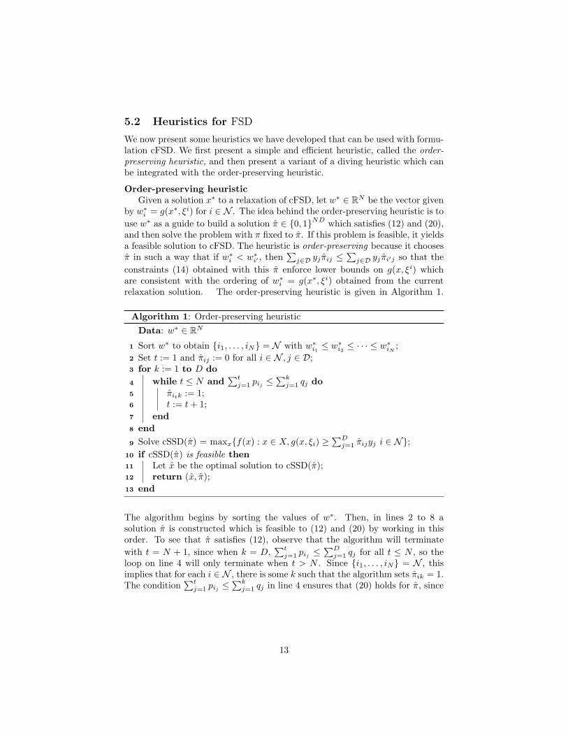
We now present some heuristics we have developed that can be used with formu-lation cFSD. We first present a simple and efficient heuristic, called the order-preserving heuristic, and then present a variant of a diving heuristic which canbe integrated with the order-preserving heuristic.

Order-preserving heuristicGiven a solution x∗ to a relaxation of cFSD, let w∗ ∈ RN be the vector given

by w∗i = g(x∗, ξi) for i ∈ N . The idea behind the order-preserving heuristic is to

use w∗ as a guide to build a solution π ∈ 0, 1ND which satisfies (12) and (20),and then solve the problem with π fixed to π. If this problem is feasible, it yieldsa feasible solution to cFSD. The heuristic is order-preserving because it choosesπ in such a way that if w∗

i < w∗i′ , then

∑j∈D yj πij ≤

∑j∈D yj πi′j so that the

constraints (14) obtained with this π enforce lower bounds on g(x, ξi) whichare consistent with the ordering of w∗

i = g(x∗, ξi) obtained from the currentrelaxation solution. The order-preserving heuristic is given in Algorithm 1.

Algorithm 1: Order-preserving heuristicData: w∗ ∈ RN

Sort w∗ to obtain i1, . . . , iN = N with w∗i1≤ w∗

i2≤ · · · ≤ w∗

iN;1

Set t := 1 and πij := 0 for all i ∈ N , j ∈ D;2

for k := 1 to D do3

while t ≤ N and∑t

j=1 pij ≤∑k

j=1 qj do4

πitk := 1;5

t := t + 1;6

end7

end8

Solve cSSD(π) = maxxf(x) : x ∈ X, g(x, ξi) ≥∑D

j=1 πijyj i ∈ N;9

if cSSD(π) is feasible then10

Let x be the optimal solution to cSSD(π);11

return (x, π);12

end13

The algorithm begins by sorting the values of w∗. Then, in lines 2 to 8 asolution π is constructed which is feasible to (12) and (20) by working in thisorder. To see that π satisfies (12), observe that the algorithm will terminatewith t = N + 1, since when k = D,

∑tj=1 pij ≤

∑Dj=1 qj for all t ≤ N , so the

loop on line 4 will only terminate when t > N . Since i1, . . . , iN = N , thisimplies that for each i ∈ N , there is some k such that the algorithm sets πik = 1.The condition

∑tj=1 pij ≤

∑kj=1 qj in line 4 ensures that (20) holds for π, since

13

it ensures that for each k ∈ D,

k∑j=1

N∑i=1

piπij =t(k)∑j=1

pij

where t(k) = max

t :∑t

j=1 pij ≤∑k

j=1 qj

.

The main work done in Algorithm 1 is the sorting of w∗, and solving ofcSSD(π). Note that this problem is small relative to the original problem cFSD,since the O(ND) variables π are fixed, the constraints (12) and (20) no longerneed to be considered, and the constraints (14) reduce to lower bounds on thefunctions g(x, ξi) for i ∈ N .

Integrated order-preserving and diving heuristicDiving is a classic heuristic strategy for integer programs which alternates

between fixing one or more integer variables based on the current linear program-ming (LP) relaxation solution and re-solving the relaxation. We have developeda variant of the diving heuristic for solving cSSD, which we call the AggressiveDiving Heuristic. For brevity, we only outline the idea of the heuristic here; fordetails, we refer the reader to [19]. Within each iteration of the aggressive divingheuristic, the heuristic repeatedly selects the index i ∈ N which has minimumvalue of w∗

i = g(x∗, ξi) and has not yet had πij fixed to one for any j ∈ D. Avariable πik is then fixed to one, where k is the minimum index such that πik

could feasibly be fixed to one and still satisfy (20). This is done until one of thefixings causes inequality (14) to be violated by the current solution, that is, untila πik is fixed to one with w∗

i < yk. Also within an iteration, a similar sequenceof fixings is done for indices i ∈ N which have maximum value of w∗

i until oneof the fixings implies (14) is violated by the current solution. After these fixingshave been done, the LP relaxation is re-solved, and the next iteration begins.The heuristic terminates when the current LP relaxation yields a feasible inte-ger solution or is infeasible (where infeasibility would be caused by the lowerbounds implied by (14) due to the fixed variables). They key advantages of theaggressive diving heuristic are that it fixes multiple variables in each iteration,leading to faster convergence, and the variables are fixed in such a way thatconstraints (12) and (20) will not become violated.

Integration of the order-preserving heuristic with the aggressive diving heuris-tic is accomplished by calling the order-preserving heuristic during each iterationof the diving heuristic, using the current relaxation solution. If this yields animproved feasible solution, it is saved, but the heuristic still continues the diveuntil it terminates. At the end, the best feasible solution found over all iterationsin the dive is reported.

6 Computational Results

We conducted computational experiments to test the new formulations forstochastic dominance. Following [17] and [25], we conducted tests on a portfolio

14

optimization problem with stochastic dominance constraints. In this problem,we wish to choose the fraction of our investment to invest in n different as-sets. The return of asset j is a random variable given by Rj with E[Rj ] = rj .We are also given a reference random variable Y and the objective is to maxi-mize the expected return subject to the constraint that the random return weachieve stochastically dominates Y . Thus, the portfolio optimization problemswe consider are

max n∑

j=1

rjxj : x ∈ X,

n∑j=1

Rjxj (k) Y

k = 1, 2 (27)

where X =x ∈ Rn

+ :∑n

j=1 xj = 1.

We constructed test instances using the daily returns of 435 stocks (n = 435)in the S&P 500, for which daily return data was available from January 2002through March 2007. We take each daily return as an outcome that occurswith equal probability. For each desired number of outcomes N , we constructedthree instances by taking the N daily returns immediately preceding March 14of the years 2005, 2006, and 2007. For example, the instance for year 2007, withN = 100 is obtained by taking the daily returns in the days from November 16,2006 through March 14, 2007.

For the reference random variable Y , we use the returns that would be ob-tained by investing an equal fraction in each of the available assets. That is, wetake Y =

∑nj=1 Rj/n. Hence, if Ri

j is the return that is achieved under outcomei for asset j, then the distribution of Y is given by νY =

∑nj=1 Ri

j/n = 1/Nfor i ∈ N . Note that in this case, the number of outcomes of Y is the sameas the number of outcomes of R, i.e., D = N . This is an extreme case: inmany settings we would expect D to be significantly less than N . However, thisextreme case will yield challenging instances for comparing the formulations.

We used CPLEX 9.0 [14] to solve the LP and MIP formulations and allexperiments were done on a computer with two 2.4 Ghz processors (althoughno parallelism is used) and 2.0 Gb of memory. The specialized heuristics andbranching for first-order stochastic dominance were implemented using callbackroutines provided by the CPLEX callable library.

6.1 Second-Order Dominance

We first compared the solution times using the formulations SDLP, cSSD1 andcSSD2 to solve the portfolio optimization problem (27) with second-order dom-inance constraint (k = 2 in (27)). We tested seven different sizes N and threeinstances for each size. These linear programs were solved using the dual sim-plex method, the default CPLEX setting, and a time limit of 100,000 secondswas used. Table 1 gives the solution time and number of simplex iterations foreach formulation on each instance. From this table it is clear that when usinga commercial LP solver, the new formulations cSSD1 and cSSD2 allow muchmore efficient solution of SSD. Formulation cSSD1 yields a solution an orderof magnitude faster than SDLP, whereas cSSD2 yields a solution roughly two

15

Table 1: Computational results for SSD formulations.

Solution Time (s) IterationsYear N SDLP cSSD1 cSSD2 SDLP cSSD1 cSSD22005 200 103 18 3 30851 10336 1921

300 1063 61 19 76438 16879 6019400 4859 127 23 118328 17692 5698500 10345 509 17 121067 34380 4770600 27734 528 39 202490 40430 5854700 69486 3366 434 318030 112848 20788800 *100122 8272 1476 *361600 222967 42773

2006 200 83 13 3 20009 7449 2134300 883 44 8 52457 12004 3244400 4253 190 25 109493 24398 5549500 11365 332 63 117559 37086 7904600 43927 670 198 307680 41360 16443700 58947 6067 94 346077 173483 13026800 *100100 10406 50 *433400 245401 6307

2007 200 122 25 9 19359 13771 4597300 757 61 30 64795 15585 8253400 4292 214 59 89731 28024 8265500 12551 609 178 154287 46973 14914600 27492 1213 271 172905 66164 18611700 59144 1888 338 308064 92365 19009800 *100095 23171 74 *385700 544342 8174

* Not solved in time limit.

16

orders of magnitude faster. Both formulation cSSD1 and cSSD2 have O(N)rows as opposed to O(ND) = O(N2) rows in SDLP, leading to a significantlyreduced basis size, so that the time per iteration using these formulations issignificantly less. The additional reduction in computation time obtained fromformulation cSSD2 can be explained by the large reduction in the number ofsimplex iterations.

We should stress that because N = D in this test, the relative improvementof cSSD1 and cSSD2 over SDLP is likely the best case. For instances in whichD is of much more modest size, such as D = 10, we would not expect suchextreme difference.

6.2 First-Order Dominance

We next present results of the tests on the portfolio optimization problem (27)in which a first-order stochastic constraint is enforced (k = 1 in (27)).

We tested four solution methods for solving FSD:

• FDMIP: Solve FDMIP with default CPLEX settings,

• cFSD: Solve cFSD with default CPLEX settings and CPLEX SOS1 branch-ing,

• cFSD+H: Solve cFSD with CPLEX SOS1 branching and specialized heuris-tic, and

• cFSD+H+B: Solve cFSD with CPLEX, specialized heuristic, and special-ized branching.

When solving cFSD with and without the heuristic (but not with the specializedbranching), we declare the sets of variables πij : j ∈ D for i ∈ N as SpecialOrdered Sets of Type 1, allowing CPLEX to perform its general purpose SOS1branching, as discussed in Section 5.1. We found that this yields better resultsthan having CPLEX perform its default single variable branching. Note thatthe specialized branching scheme also uses SOS1 branching, but crucially differsfrom the CPLEX implementation in the selection of the SOS1 set and level tobranch on.

The heuristic used in the last two methods is the aggressive diving heuristicintegrated with the order-preserving heuristic. In our implementation, we callthe heuristic at every node of depth less than five, at every fifth node for the first100 nodes, at every 20th node between 100 and 1000 nodes, and at every 100thnode thereafter. When the heuristic is used we turn off the CPLEX heuris-tics and preprocessing. The preprocessing was turned off for implementationconvenience, but we found it had little effect for formulation cFSD anyway.

The specialized branching used in the last method is the branching strategygiven in Section 5.1. For this case, we set the CPLEX branching variable selec-tion to select the most fractional variable since this takes the least time and wedo not use CPLEX’s choice of branching variable anyway.

17

We first compare the time to solve the root linear program relaxations andthe resulting lower bound from formulations FDMIP and cFSD. These resultsare given in Table 2. For formulation FDMIP we report the results beforeand after addition of CPLEX cuts. The results obtained after the addition ofCPLEX cuts are under the column FDMIP.C. For cFSD, we report only theresults after the initial relaxation solution, because CPLEX cuts had little effectin this formulation. For formulation FDMIP we report the percent by which the

Table 2: Comparison of root LP relaxations for FSD formulations.

Time (s) Percent above cFSD UBYear N cFSD FDMIP FDMIP.C FDMIP FDMIP.C2005 100 1.0 6.6 41.4 5.36% 3.46%

150 1.8 19.7 89.5 7.64% 6.18%200 4.7 36.3 196.2 8.42% 5.87%250 15.1 49.9 365.0 9.34% 6.78%300 31.0 232.6 681.5 9.78% 7.50%350 88.0 509.7 1201.0 4.36% 3.05%400 97.6 427.7 1566.2 5.14% 3.19%

2006 100 0.4 3.9 4.3 0.21% 0.00%150 3.8 16.2 82.0 1.54% 1.03%200 4.8 26.3 140.9 1.38% 1.08%250 17.5 91.1 325.8 3.99% 2.45%300 16.4 191.3 575.6 4.60% 3.53%350 52.3 227.7 1157.8 8.49% 6.52%400 69.1 1254.7 2188.6 6.92% 5.77%

2007 100 2.0 4.5 33.5 7.55% 3.70%150 8.1 17.0 148.4 7.69% 6.06%200 17.8 33.3 300.8 9.75% 8.26%250 36.1 121.4 413.1 14.13% 10.71%300 43.5 298.6 732.6 11.12% 8.26%350 114.0 320.9 1060.7 10.80% 10.60%400 245.7 2010.8 3664.2 11.53% 11.02%

upper bound (UB) obtained from the relaxation with and without cuts exceedsthe upper bound obtained from the relaxation of cFSD. It is clear from Table2 that the relaxation of formulation cFSD provides significantly better upperbounds in significantly less time.

We next tested how the different methods performed when run for a timelimit of 10,000 seconds. Table 3 reports the optimality gap remaining after thistime limit. All formulations were able to solve the 2006 instance with N = 100in less than a minute, so this instance is excluded. Using formulation cFSDwith the heuristic and specialized branching, 8 of the remaining 20 instanceswere solved to optimality within the time limit, and for these instances the

18

solution time is reported (these are the instances with ‘-’ in the “Gap” column).From Table 3 we observe that even without the use of specialized heuristic

Table 3: Comparison of optimality gaps for FSD after time limit.

Optimality Gap cFSD+H+BYear N FDMIP cFSD cFSD+H Gap Time (s)2005 100 1.69% 0.68% 0.68% - 864.0

150 2.84% 0.99% 0.73% - 223.1200 4.46% 1.09% 0.87% - 1987.3250 8.82% 0.31% 0.24% - 2106.6300 ** 3.41% 1.21% 1.15%350 ** ** 2.15% 1.39%400 ** 10.67% 0.73% 0.31%

2006 150 1.71% 0.77% 0.55% 0.18%200 1.25% 0.57% 0.55% - 1752.1250 4.82% 0.97% 0.44% - 274.9300 4.56% 4.24% 0.85% - 9386.8350 ** 1.96% 0.65% 0.53%400 ** 4.77% 1.21% 0.87%

2007 100 0.13% 0.14% 0.15% - 41.6150 13.90% 4.11% 2.37% 1.85%200 ** 3.80% 1.64% 0.67%250 ** 9.13% 2.12% 0.67%300 ** ** 2.43% 2.01%350 ** ** 6.74% 6.37%400 ** ** 5.82% 5.79%

** No feasible solution found.

or branching formulation cFSD outperforms formulation FDMIP. However, inseveral instances cFSD fails to find a feasible solution, and in several others theoptimality gaps for the feasible solutions found are quite bad. This is remediedto a significant extent by using the specialized heuristic, in which case a feasiblesolution is found for every instance, and in most cases it is within 2% of theupper bound. If, in addition, we use the specialized branching scheme, the finaloptimality gaps are reduced even further, with many of the instances beingsolved to optimality.

Table 4 gives more detailed results for the methods based on formulationcFSD for the 2005 instances (results for the other instances yield similar in-sights and are excluded for brevity). First, for each of these methods, the tableindicates the percent by which the final upper bound (UB) was below the initialupper bound (Root UB) obtained simply from solving the linear programmingrelaxation. These results indicate that by using CPLEX branching, with andwithout the specialized heuristic, very little progress is made in improving the

19

upper bound through branching. In contrast, the specialized branching schemeimproves the upper bound considerably. Table 4 also reports the percent by

Table 4: Lower and upper bounds results using cFSD.

% UB below Root UB % LB below Best UBYear N cFSD +H +H+B cFSD +H +H+B2005 100 0.02% 0.02% 0.69% 0.01% 0.01% 0.01%

150 0.00% 0.00% 0.66% 0.33% 0.07% 0.01%200 0.00% 0.00% 0.74% 0.36% 0.14% 0.01%250 0.00% 0.00% 0.20% 0.11% 0.04% 0.01%300 0.00% 0.00% 0.06% 3.47% 1.17% 1.16%350 0.00% 0.00% 0.26% ** 1.93% 1.41%400 0.00% 0.00% 0.23% 11.68% 0.50% 0.31%

** No feasible solution found.

which the value of the best feasible solution found (LB) is below the best upperbound found over all methods (Best UB). These results indicate that the spe-cialized heuristic significantly improves the value of the feasible solutions found,and that integrating the specialized branching with the heuristic often yieldseven further improvement in solution quality.

7 Concluding Remarks

More computational experiments need to be performed to test the effectivenessof the new formulations in different settings. For example, we tested the case inwhich the number of possible realizations of the reference random variable, D, islarge. The case in which D is small should also be tested since this is likely thecase when a stochastic dominance constraint is used to model a collection of riskconstraints. It would be particularly interesting to test these formulations forradiation treatment planning models with dose-volume constraints. We expectthat when D is small it will be possible to significantly increase the numberof possible realizations, N , of the random vector appearing in the constraints.Another setting in which to test the new formulations is in two-stage stochasticprogramming with stochastic dominance constraints, as has been recently stud-ied in [11, 12], where they use the previous, less compact, formulations for thestochastic dominance constraints.

Finally, it will be interesting to study a Monte Carlo sampling based ap-proximation scheme for problems with stochastic dominance constraints havingmore general distributions. Results on sample approximations for probabilisticconstraints (e.g. [3, 20, 23]) may be applied to yield approximations for first-order stochastic dominance constraints in which the random vector ξ appearingin the constraint may have general distribution. It will be interesting to explorewhether the specific structure of the first-order stochastic dominance constraint

20

can yield results beyond direct application of the results for probabilistic con-straints. Similarly, results on sample approximations for optimization problemswith expected value constraints (e.g. [27, 28]) may be applied to yield approxi-mations for second-order dominance constraints.

Acknowledgements

The author is grateful to Shabbir Ahmed for his helpful comments on a draft ofthis paper. The author also thanks Darinka Dentcheva, Andrzej Ruszczynski,and an anonymous referee for pointing out the connection between the SSDformulations presented and Strassen’s theorem.

References

[1] E. Balas, Disjunctive programming: Properties of the convex hull of fea-sible points., Discrete Appl. Math., 89 (1998), pp. 3–44.

[2] E. Beale and J. Tomlin, Special facilities in a general mathematical pro-gramming system for non-convex problems using ordered sets of variables,in Proc. Fifth Internat. Conf. on OR, J. Lawrence, ed., London, UK, 1970,Tavistock Publications, pp. 447–454.

[3] G. Calafiore and M. Campi, The scenario approach to robust controldesign, IEEE Trans. Automat. Control, 51 (2006), pp. 742–753.

[4] D. Dentcheva and A. Ruszczynski, Optimization with stochastic dom-inance constraints, SIAM J. Optim., 14 (2003), pp. 548–566.

[5] , Optimality and duality theory for stochastic optimization problemswith nonlinear dominance constraints, Math. Program., 99 (2004), pp. 329–350.

[6] , Semi-infinite probabilistic optimization: first-order stochastic domi-nance constraints, Optimization, 53 (2004), pp. 583–601.

[7] , Portfolio optimization with stochastic dominance constraints, Jour-nal of Banking & Finance, 30 (2006), pp. 433–451.

[8] C. Fabian, G. Mitra, and D. Roman, Processing second-order stochas-tic dominance models using cutting-plane representations. CARISMA Tech-nical Report CTR/75/08, 2008.

[9] J. Forrest, D. de la Nuez, and R. Lougee-Heimer, CLP User Guide,2004.

[10] R. Gollmer, U. Gotzes, F. Neise, and R. Schultz, Risk model-ing via stochastic dominance in power systems with dispersed generation,Tech. Rep. Preprint 651/2007, Department of Mathematics, University ofDuisburg-Essen, 2007. www.uni-duisburg.de/FB11/disma/preprints.shtml.

21

[11] R. Gollmer, U. Gotzes, and R. Schultz, Second-order stochasticdominance constraints induced by mixed-integer linear recourse, Tech. Rep.Preprint 644/2007, Department of Mathematics, University of Duisburg-Essen, 2007. www.uni-duisburg.de/FB11/disma/preprints.shtml.

[12] R. Gollmer, F. Neise, and R. Schultz, Stochastic programs withfirst-order dominance constraints induced by mixed-integer linear recourse,Tech. Rep. Preprint 641/2006, Department of Mathematics, University ofDuisburg-Essen, 2006. www.uni-duisburg.de/FB11/disma/preprints.shtml.

[13] G. Hardy, J. Littlewood, and G. Polya, Inequalities, CambridgeUniversity Press, 1934.

[14] Ilog, Ilog CPLEX 9.0 User’s Manual, 2003.

[15] W. K. Klein Haneveld, Duality in Stochastic Linear and Dynamic Pro-gramming, vol. 274 of Lecture Notes in Economics and Math. Systems,Springer-Verlag, New York, NY, 1986.

[16] W. K. Klein Haneveld and M. H. van der Vlerk, Integrated chanceconstraints: reduced forms and an algorithm, Comput. Manage. Sci., 3(2006), pp. 245–269.

[17] T. Kuosmanen, Efficient diversification according to stocastic dominancecriteria, Manage. Sci., 50 (2004), pp. 1390–1406.

[18] E. Lee, T. Fox, and I. Crocker, Integer programming applied tointensity-modulated radiation therapy treatment planning, Ann. Oper. Res.,119 (2003), pp. 165–181.

[19] J. Luedtke, Integer Programming Approaches to Some Non-convex andStochatic Optimization Problems, PhD thesis, Georgia Institute of Tech-nology, Atlanta, GA, 2007. Available online at etd.gatech.edu.

[20] J. Luedtke and S. Ahmed, A sample approximation approach for opti-mization with probabilistic constraints, SIAM J. Optim., (2008). To appear.

[21] A. Marshall and I. Olkin, Inequalities: Theory of Majorization, Aca-demic Press, New York, 1979.

[22] A. Muller and D. Stoyan, Comparison Methods for Stochastic Modelsand Risks, John Wiley & Sons, LTD, Chichester, England, 2002.

[23] A. Nemirovski and A. Shapiro, Scenario approximation of chance con-straints, in Probabilistic and Randomized Methods for Design Under Uncer-tainty, G. Calafiore and F. Dabbene, eds., Springer, London, 2005, pp. 3–48.

[24] N. Noyan, G. Rudolf, and A. Ruszczynski, Relaxations of linearprogramming problems with first order stochastic dominance constraints,Oper. Res. Lett., 34 (2006), pp. 653–659.

22

[25] N. Noyan and A. Ruszczynski, Valid inequalities and restrictions forstochastic programming problems with first order stochastic dominance con-straints, Math. Program., 114 (2008), pp. 249–275.

[26] G. Rudolf and A. Ruszczynski, Optimization problems with secondorder stochastic dominance constraints: duality, compact formulations, andcut generation methods. RUTCOR Research Report, Rutgers University,Piscataway, NJ, 2007.

[27] A. Shapiro, Asymptotic behavior of optimal solutions in stochastic pro-gramming, Math. Oper. Res., 18 (1993), pp. 829–845.

[28] W. Wang and S. Ahmed, Sample average approximation of expected valueconstrained stochastic programs. Preprint available at www.optimization-online.org, 2007.

[29] G. Whitmore and M. Findlay, eds., Stochastic Dominance, D.C. Heathand Company, Lexington, MA, 1978.

23