Multiwaveband polarimetric observations of 15 active ...

Physics

Physics Research Publications

Purdue University Year

Multiwaveband polarimetric observations

of 15 active galactic nuclei at high

frequencies: Correlated polarization

behaviorS. G. Jorstad, A. P. Marscher, J. A. Stevens, P. S. Smith, J. R. Forster, W. K.Gear, T. V. Cawthorne, M. L. Lister, A. M. Stirling, J. L. Gomez, J. S. Greaves,and E. I. Robson

This paper is posted at Purdue e-Pubs.

http://docs.lib.purdue.edu/physics articles/635

MULTIWAVEBAND POLARIMETRIC OBSERVATIONS OF 15 ACTIVE GALACTIC NUCLEIAT HIGH FREQUENCIES: CORRELATED POLARIZATION BEHAVIOR

Svetlana G. Jorstad,1,2

Alan P. Marscher,1Jason A. Stevens,

3Paul S. Smith,

4James R. Forster,

5

Walter K. Gear,6Timothy V. Cawthorne,

7Matthew L. Lister,

8Alastair M. Stirling,

9

Jose L. Gomez,10

Jane S. Greaves,11

and E. Ian Robson12

Received 2007 March 7; accepted 2007 May 16

ABSTRACT

We report onmultifrequency linear polarization monitoring of 15 active galactic nuclei containing highly relativisticjets with apparent speeds from�4c to >40c. Themeasurementswere obtained at optical, 1mm, and 3mmwavelengths,and at 7 mmwith the Very Long Baseline Array. The data show a wide range in degree of linear polarization amongthe sources, from<1% to >30%, and interday polarization variability in individual sources. The polarization propertiessuggest separation of the sample into three groups with low, intermediate, and high variability of polarization in thecore at 7 mm (LVP, IVP, and HVP, respectively). The groups are partially associated with the common classificationof active galactic nuclei as radio galaxies and quasars with low optical polarization (LVP), BL Lacertae objects (IVP),and highly optically polarized quasars (HVP). Our study investigates correlations between total flux, fractionalpolarization, and polarization position angle at the different wavelengths.We interpret the polarization properties ofthe sources in the sample through models in which weak shocks compress turbulent plasma in the jet. The differencesin the orientation of sources with respect to the observer, jet kinematics, and abundance of thermal matter external tothe jet near the core can account for the diversity in the polarization properties. The results provide strong evidencethat the optical polarized emission originates in shocks, most likely situated between the 3 and 7 mmVLBI cores. Theyalso support the idea that the 1 mm core lies at the edge of the transition zone between electromagnetically dominatedand turbulent hydrodynamic sections of the jet.

Key words: BL Lacertae objects: individual (1803+784, 1823+568, 3C 66A, BL Lac, OJ 287) —galaxies: active — galaxies: individual (3C 111, 3C 120) — galaxies: jets — polarization —quasars: individual (0420�014, 0528+134, 3C 273, 3C 279, 3C 345, 3C 454.3, CTA 102,PKS 1510�089)

Online material: machine-readable tables

1. INTRODUCTION

Magnetic fields play a prominent role in the physical processesthat occur in the jets of active galactic nuclei (AGNs). The leadingmodel for jet production, acceleration, and collimation involvespoloidal magnetic fields that are wound up by the differential ro-tation of a rotating disk or ergosphere surrounding a central super-massive black hole (e.g., McKinney 2006; Meier et al. 2001).

The twisted field propagates outward as Poynting flux in the polardirections, with eventual conversion into a well-focused rela-tivistic plasma flow (e.g., Vlahakis & Konigl 2004; Meier &Nakamura 2006). Within this zone, the magnetic field shouldmaintain a tight helical pattern.

Beyond the jet acceleration region—which may extend overhundreds or thousands of gravitational radii from the black hole(Vlahakis & Konigl 2004; Marscher 2006)—the jet may be-come turbulent or subject to velocity shear. In the former case,themagnetic field should be chaotic, with any line of sight passingthrough many turbulent cells and significant differences in bothstrength and direction of the field in adjacent cells. In contrast,velocity shear stretches and orders the field lines along the flow(e.g., Laing 1980). Shockwaves passing through the flow (or viceversa) will compress the component of the field that is parallel tothe shock front, which imposes order even on amagnetic field thatis completely chaotic in front of the shock.

The geometry and degree of order of the magnetic field aretherefore key indicators of the physical conditions in a jet. Be-cause the primary emission mechanism at radio to optical wave-lengths is synchrotron radiation, the linear polarization of thecontinuum can be used as a probe of the magnetic field. We canalso use the fractional polarization and direction of the electricvector position angle (EVPA) to identify distinct features in thejet that are observed at different wavelengths. Themost prominentfeatures on VLBI images of jets in radio-loud AGNs are (1) thecore, which is the bright, very compact section at the narrow endof a one-sided jet, and (2) condensations in the flow that appearas bright knots, often called ‘‘components’’ of the jet. The core

A

1 Institute for Astrophysical Research, Boston University, 725 CommonwealthAvenue, Boston, MA 02215-1401, USA; [email protected], [email protected].

2 SobolevAstronomical Institute, St. Petersburg State University, UniversitetskijProspekt 28, 198504 St. Petersburg, Russia.

3 Centre forAstrophysics Research, Science andTechnologyCentre,Universityof Hertfordshire, College Lane, Herts AL10 9AB, UK; [email protected].

4 Steward Observatory, The University of Arizona, Tucson, AZ 85721, USA;[email protected].

5 Hat Creek Observatory, University of California, Berkeley, 42231 BidwellRoad, Hatcreek, CA 96040, USA; [email protected].

6 School of Physics and Astronomy, Cardiff University, 5, The Parade, CardiffCF2 3YB, Wales, UK; [email protected].

7 Centre for Astrophysics, University of Central Lancashire, Preston PR1 2HE,UK; [email protected].

8 Department of Physics, PurdueUniversity, 525NorthwesternAvenue,WestLafayette, IN 47907-2036, USA; [email protected].

9 Jodrell Bank Observatory, University of Manchester, Macclesfield, CheshireSK11 9DL, UK; [email protected].

10 Insituto deAstrof ısica deAndalucıa (CSIC), Apartado 3004,Granada 18080,Spain; [email protected].

11 School of Physics andAstronomy, University of St. Andrews,North Haugh,St. Andrews, Fife KY16 9SS, UK; [email protected].

12 AstronomyTechnologyCentre, Royal Observatory, BlackfordHill, EdinburghEH9 3HJ, UK; [email protected].

799

The Astronomical Journal, 134:799Y824, 2007 August

# 2007. The American Astronomical Society. All rights reserved. Printed in U.S.A.

likely lies some distance from the central engine of the AGN,probably either near the end or beyond the zone of accelerationand collimation of the jet (Marscher 2006). The knots usuallyseparate from the core at apparent superluminal speeds, but roughlystationary knots are also present in many jets, perhaps represent-ing standing shocks (e.g., Jorstad et al. 2001, 2005, hereafter J05;Kellermann et al. 2004; Lister 2006). The apparent speeds ofthe components can exceed �app � 40c (J05), which requires thatthe Lorentz factor of the flow exceeds �app. The leading modelidentifies the moving knots as propagating shocks, either trans-verse to the jet axis (e.g., Hughes et al. 1985, 1989; Marscher &Gear 1985) or at an oblique angle (Hughes 2005). Polarizationstudies can help to determine whether this model is viable.

The standard paradigm of transverse shocks propagating downa relativistic jet can explain many aspects of the time variabilityof the brightness, polarization, and structure at radio wavelengths(e.g., Hughes et al. 1985, 1989; Cawthorne&Wardle 1988;Wardleet al. 1994). However, this model makes predictions—e.g., that themagnetic field of a knot should be transverse to the jet axis—thatoften do not match observations. Another possibility is that thereis a systematically ordered component of the magnetic field, forexample one with a helical geometry (e.g., Lyutikov et al. 2005),in the jet that modulates its brightness and polarization variabil-ity. In fact, a helical magnetic field is required in the magneto-hydrodynamic jet launching models (Meier et al. 2001; Vlahakis&Konigl 2004).Gabuzda (2006) provided some support for sucha geometry in recent low-frequencyVLBI observations of Faradayrotation in AGN jets. However, this structure can be related tothe magnetic field in the Faraday screen surrounding the jet sincehigh-frequency radio polarization mapping reveals aspects thatare difficult to explain by a helical field (Hughes 2005; Zavala &Taylor 2005).

The situation is even more confusing in the optical and near-IRregions, where variations in flux and polarization are often ex-tremely rapid, and submilliarcsecond resolution is not available(e.g., Hagen-Thorn 1980; Moore et al. 1987; Smith et al. 1987;Mead et al. 1990). Furthermore, existing optical data indicatethat the connection between variations in brightness and polariza-tion is tenuous (e.g., Smith 1996). These factors complicate inter-pretation of the optical /near-IR emission, since detailedmodelsare needed but the data are not extensive enough to guide them.An alternative approach is to investigate the global polarizationbehavior across a sizable range of the electromagnetic spectrum.Such studies (Wills et al. 1992; Gabuzda et al. 1996, 2006; Lister& Smith 2000) have produced convincing evidence for a con-nection between the radio and optical polarization properties ofAGNs, suggestive of a common, probably cospatial, origin forthe emission at these two wave bands. However, such studieshave been based on single-epoch measurements, whereas theinvestigation we present here involves multiepoch observationsof 15 objects. This allows us to use both the time and frequencydomains to explore the geometry and degree of ordering of themagnetic field and other properties of the emission regions in rel-ativistic jets.

Bright jets with high apparent superluminal motion are a prev-alent feature of blazars, a classification that includes BL Lac ob-jects and optically violently variable quasars (OVVs) that arequite rare in the general AGNpopulation (Kellermann et al. 2004;Lister 2006). The prominence of the jets from radio to opticalwavelengths and the pronounced variability of their polarizedemission makes blazars and radio galaxies with blazar-like be-havior ideal objects for probing the magnetic fields in jets throughmultiepoch polarization studies.

We have carried out a 3 yr monitoring program of 15 radio-loud, highly variable AGNs. The program combines roughlybimonthly, high-resolution polarized and total-intensity radioimages with optical, submillimeter-wave, and millimeter-wavepolarization observations performed at many of the same epochs.The sample includes objects that are usually brighter than about2 Jy at 7 mm and 1 Jy at 1 mm, with a mixture of quasars (0420�014, 0528+134, 3C 273, 3C 279, 1510�089, 3C 345, CTA 102,and 3C 454.3), BL Lac objects (3C 66A, OJ 287, 1803+784,1823+568, and BL Lac), and radio galaxies with bright compactradio jets (3C 111 and 3C 120). In J05, we investigated the prop-erties of the jets on milliarcsecond scales and determined the ap-parent velocities of more than 100 jet features. For the majorityof these components, we derived Doppler factors using a newmethod based on comparison of the timescale of decline in fluxdensity with the light travel time across the emitting region. Thisallowed us to estimate the Lorentz factors, as well as viewing andopening angles for the jets of all of the sources in our sample.Here we apply these parameters in our interpetation of the multi-frequency polarization properties of the sources. Because of dif-ficulties in coordinating the schedules at the different telescopes,our observations at different wavelengths are contemporaneous(within 2 days to 2 weeks of each other) rather than exactly simul-taneous. Nevertheless, the program provides the richest multi-epoch, multiYwave band polarization data set compiled to date.

2. OBSERVATIONS AND DATA REDUCTION

We have measured the total flux densities and polarizationof the objects in our sample in four spectral regions: at 7 mm(43 GHz), 3 mm (86 GHz), 0.85/1.3 mm (350/230 GHz), andoptical wavelengths (an effective wavelength of �600Y700 nm).

2.1. Optical Polarization Observations

We carried out optical polarization and photometric mea-surements at several epochs using the Two-Holer Polarimeter/Photometer (Sitko et al. 1985) with the Steward Observatory1.5 m telescope located on Mount Lemmon, Arizona, and the1.55 m telescope on Mount Bigelow, Arizona. This instrumentuses a semiachromatic half-wave plate spinning at 20.65 Hz tomodulate incident polarization and a Wollaston prism to directorthogonally polarized beams to two RCA C31034 GaAs photo-multiplier tubes. For all polarization measurements we usedeither a 4.300 or 8.000 circular aperture and, except for 3C 273, nofilter. The unfiltered observations sample the polarization between�320 and 890 nm,with an effective central wavelength of �600Y700 nm, depending on the spectral shape of the observed object.In the case of 3C 273 a Kron-Cousins R filter (keA � 640 nm)was employed to avoid major unpolarized emission-line features(Smith et al. 1993). We accomplished sky subtraction by noddingthe telescope to a nearby (<3000), blank patch of sky several timesduring each observation. Data reduction of the polarimetry fol-lowed the procedure described in Smith et al. (1992).When conditions were photometric, we obtained differential

V-band photometry (R-band photometry in the case of 3C 273) ofseveral objects, employing either an 8.000 or 16.000 circular aper-ture.We used comparison stars in the fields of the AGNs (Smithet al. 1985; Smith & Balonek 1998) to calibrate nearly all of thephotometry. We determined the V magnitudes of 3C 111 and3C 120 on 1999 February 13 from the photometric solution pro-vided by observations of equatorial standard stars (Landolt 1983).Table 1 lists the results of the optical observations. The columns

correspond to (1) source, (2) epoch of observation, (3) filter band-pass of the photometry, (4) apparent magnitude, (5) flux density,

JORSTAD ET AL.800 Vol. 134

Iopt, (6) filter bandpass of the polarimetry, where W denotes un-filtered, or ‘‘white-light’’ measurements, (7) degree of linear po-larization, mopt, and (8) polarization position angle �opt. We havecorrected the degree of linear polarization for the statistical biasinherent in this positive-definite quantity by using the methodof Wardle & Kronberg (1974). Usually this correction is neg-ligible because of the high signal-to-noise ratio (S/N) of mostmeasurements.

Because of the high observed optical polarization levels andhigh Galactic latitudes of the majority of the sources, interstellarpolarization (ISP) is not a significant concern in most cases. Inter-stellar polarization from dust within the Milky Way galaxy doesappear to be a major component of the observed optical polar-ization for 3C 111 (b ¼ �8:8�) and 3C 120 (b ¼ �27:4�). A star�5000 west of 3C 111 shows very high polarization (m ¼ 3:6% �0:2%; � ¼ 123� � 2�); this was used to correct the polarimetryfor ISP in the line of sight to the radio galaxy. The corrected mea-surements suggest that the intrinsic polarization of 3C 111 wastypically <3% throughout the monitoring campaign. The aver-age polarization for five stars within 80 of 3C 120 yields m ¼1:22% � 0:06% and � ¼ 98� � 1�. We have used this ISP esti-mate to correct the observed polarization of 3C 120 for interstellarpolarization and, as for 3C 111, list the corrected measurementsin Table 1. The corrected values indicate that 3C 120 had very lowpolarization (mopt < 0:5%) throughout the monitoring program.

Impey et al. (1989) have determined the interstellar polariza-tion along the line of sight to 3C 273 to be small, but the lowlevels of polarization observed for this quasar require that thisestimate of the ISP be subtracted from the R-band measurements.Table 1 lists the corrected polarization for 3C 273.

2.2. Submillimeter Polarization Observations

We performed observations at 1.35 and 0.85 mm with theJames Clerk Maxwell Telescope (JCMT) located on Mauna Kea,Hawaii using the Submillimeter Common User Bolometer Array(SCUBA; Holland et al. 1999) and its polarimeter (Greaves et al.2003). The initial plan was to observe exclusively at 1.35 mmbecause the sources are almost always brighter, the atmosphericopacity is lower, and the sky is more stable than at 0.85 mm.However, failure of the SCUBA filter drum in 1999 November

forced a switch to 0.85 mm thereafter. The polarization propertiesof blazars tend to be very similar at millimeter and submillimeterwavelengths (Nartallo et al. 1998), so the modest change inwave-length should not affect our analysis. For convenience we referto the data obtained with the JCMT as 1 mm data.

The SCUBA polarimeter consists of a rotating quartz half-wave plate and a fixed analyzer. During an observation, the wave-plate is stepped through 16 positions, and photometric data aretaken at each position. One rotation takes �360 s to complete,and the procedure results in a sinusoidally modulated signal fromwhich the Stokes parameters are extracted. A typical observa-tion consists of 5Y10 complete rotations of the waveplate. Weachieved flux calibration in the standard manner with observa-tions of planets or JCMTsecondary calibrators. We measured theinstrumental polarization (�1%) during each run by making ob-servations of a compact planet, usually Uranus, which is assumedto be unpolarized at millimeter/submillimeter wavelengths.

We performed the initial (nod compensation, flat-field, extinc-tion correction, and sky noise removal, if appropriate) and po-larimetric stages of the data reduction using the standard SCUBAdata reduction packages SURF and SIT.13 The Stokes parameterswere extracted by fitting sinusoids to the data, either half cycle(8 points), resulting in two estimates, or full cycle (16 points),yielding only one estimate but generally giving better results withnoisy data. We removed spurious measurements by performing aKolmogorov-Smirnov test on the collated data and then calculatedthe degree and position angle of the polarization, corrected for in-strumental polarization and parallactic angle. Table 2 lists the data,with the columns corresponding to (1) source, (2) epoch of obser-vation, (3) wavelength k, (4) flux density I1 mm, (5) degree of lin-ear polarization m1 mm, and (6) polarization position angle �1 mm.As with the optical measurements, the values of m1 mm have beencorrected for statistical bias.

2.3. 3 mm Polarization Observations

From 2000 April to 2001 April we monitored the sources at86 GHz using the linear polarization system on the the Berkeley-Illinois-Maryland Array (BIMA) in Hat Creek, California during

TABLE 1

Optical Polarization Data

Source

(1)

Epoch

(2)

Photometry Filter

(3)

Mag

(4)

Iopt(mJy)

(5)

Polarimetry Filter

(6)

mopt

(%)

(7)

�opt

(deg)

(8)

3C 66A............... 1999 Feb 12 . . . . . . . . . W 13.8 � 0.2 37.2 � 0.3

1999 Feb 13 V 14.70 � 0.02 4.81 � 0.08 W 13.3 � 0.2 45.2 � 0.4

1999 Feb 14 V 14.74 � 0.02 4.63 � 0.08 W 14.5 � 0.2 47.4 � 0.3

2000 Sep 27 V 14.78 � 0.02 4.46 � 0.08 W 29.7 � 0.2 17.2 � 0.2

2000 Sep 28 V 14.81 � 0.02 4.35 � 0.09 W 26.8 � 0.3 17.1 � 0.4

2000 Sep 29 . . . . . . . . . W 24.2 � 0.3 13.4 � 0.4

2000 Nov 30 V 14.40 � 0.02 6.31 � 0.11 W 23.7 � 0.1 25.4 � 0.1

2000 Dec 1 . . . . . . . . . W 22.8 � 0.2 25.1 � 0.2

2001 Jan 19 V 14.43 � 0.02 6.16 � 0.10 W 24.6 � 0.1 10.1 � 0.1

3C 111................ 1999 Feb 13 V 18.95 � 0.12 0.10 � 0.02 W 3.1 � 0.8 126 � 4

2000 Apr 3 . . . . . . . . . W 0.8 � 0.8 106 � 5

2000 Sep 27 . . . . . . . . . W 1.5 � 0.6 104 � 3

2000 Nov 30 . . . . . . . . . W 1.9 � 0.5 131 � 3

2000 Dec 1 . . . . . . . . . W 1.6 � 0.8 110 � 5

2001 Jan 19 . . . . . . . . . W 1.3 � 0.4 89 � 3

Note.—Table 1 is published in its entirety in the electronic edition of the Astronomical Journal. A portion is shown here for guidance regarding its form and content.

13 See http://www.jach.hawaii.edu/JCMT/continuum/data/reduce.html.

MULTIFREQUENCY POLARIZATION OBSERVATIONS 801No. 2, 2007

unsubscribed telescope time. The data quality was quite variable,and typical total integration times were about 10 minutes persource. We omit from our analysis data taken during extremelyhigh atmospheric phase variations or bad opacity conditions.We observed planets (Mars, Uranus, and Venus), H ii regions(W3OH andMWC349), and 3C84 as quality checks and for fluxcalibration.

We analyzed the data by mapping all four Stokes parametersfor each sideband separately, producing images of total intensity,linearly polarized flux density, degree of polarization, and polar-ization position angle for each source at each epoch. Data havingS/N < 3 for both the total and linearly polarized intensity imagesat the central pixel of the source were omitted.We determined thetotal and polarized flux densities by fitting a Gaussian brightnessdistribution to the corresponding image. Table 3 contains theresults of the observations after correction of the degree of polar-ization for statistical bias; the columns are (1) source, (2) epochof observation, (3) flux density I3 mm, (4) degree of linear polar-ization m3 mm, and (5) polarization position angle �3 mm.

2.4. 7 mm VLBA Observations

We performed total and polarized intensity imaging at 43 GHzwith the Very Long Baseline Array (VLBA) at 17 epochs from1998 March 25 to 2001 April 14. We describe the observationsand data reduction in detail in J05, where the total and polarizedintensity images are presented. Table 4 gives the results of fittingthe VLBI core seen in the total and polarized intensity images bycomponents with circular Gaussian brightness distributions (seeJ05). Columns of the table are as follows: (1) source, (2) epochof observation, (3) flux density in the core I7 mm, (4) projectedinner jet direction �jet, (5) degree of linear polarization in thecore m7 mm, and (6) polarization position angle in the core �7 mm.We determine the projected inner jet direction from the position of

the brightest jet component closest to, but at least one synthesizedbeam width from, the core.Table 5 gives the polarization of jet components downstream

of the VLBI core that are either brighter than or comparable tothe core at least at one epoch (I comp � 0:5I7 mm) or have detect-able polarization at three or more epochs. These data allow us toprobe the physics of the strongest disturbances that propagatedown the jet. The columns of Table 5 are: (1) source, (2) epochof observation, (3) designation of the component, which followsthat of J05, (4) flux density in the component I

comp7 mm , (5) distance

from the coreR, (6) position angle relative to the core�, (7) degree

TABLE 2

JCMT Polarization Data

Source

(1)

Epoch

(2)

k(mm)

(3)

I1 mm

(Jy)

(4)

m1 mm

(%)

(5)

�1 mm

(deg)

(6)

3C 66A................. 1998 May 15 1.35 0.38 � 0.04 36 � 4 24 � 2

1998 Jul 17 1.35 0.41 � 0.04 19 � 4 176 � 6

1998 Sep 30 1.35 0.45 � 0.04 14 � 2 56 � 4

1998 Nov 23 1.35 0.41 � 0.04 (11 � 5) (172 � 10)

1998 Dec 13 1.35 0.47 � 0.05 14 � 2 38 � 4

1999 Feb 18 1.35 0.43 � 0.04 11 � 2 157 � 4

1999 Apr 22 1.35 0.48 � 0.04 9.3 � 2.5 134 � 7

1999 Sep 23 1.35 0.59 � 0.06 9.7 � 2.5 158 � 10

2000 Jun 8 0.85 0.61 � 0.06 9.6 � 1.3 9 � 4

2001 Jan 17 0.85 0.61 � 0.06 11 � 2 23 � 4

2001 Jan 23 0.85 0.59 � 0.06 14 � 3 4 � 5

3C 111.................. 1998 Jul 17 1.35 1.03 � 0.10 12 � 2 39 � 4

1998 Nov 30 1.35 1.45 � 0.10 3.9 � 0.7 117 � 5

1998 Nov 23 1.35 1.26 � 0.13 4.2 � 0.9 123 � 6

1998 Dec 13 1.35 1.37 � 0.14 5.8 � 1.6 39 � 7

1999 Feb 18 1.35 1.04 � 0.10 4.5 � 1.1 126 � 6

1999 Nov 23 1.35 0.89 � 0.09 6.4 � 2.0 143 � 11

1999 Dec 24 0.85 0.93 � 0.10 (4.9 � 1.9) (17 � 10)

2000 Jun 8 0.85 1.05 � 0.11 (1.0 � 1.5) (144 � 39)

2001 Jan 17 0.85 3.61 � 0.36 2.2 � 0.7 46 � 8

2001 Jan 23 0.85 5.99 � 0.60 1.0 � 0.3 17 � 7

Note.—Table 2 is published in its entirety in the electronic edition of the Astronomical Journal. A portion isshown here for guidance regarding its form and content.

TABLE 3

BIMA Polarization Data

Source

(1)

Epoch

(2)

I3 mm

(Jy)

(3)

m3 mm

(%)

(4)

�3 mm

(deg)

(5)

3C 66A........ 2000 Apr 21 0.82 � 0.01 3.5 � 0.7 171 � 5

2000 Apr 25 0.98 � 0.01 5.0 � 0.5 1 � 2

2001 Feb 6 0.89 � 0.01 9.3 � 0.3 17 � 1

2001 Mar 20 0.65 � 0.01 4.2 � 0.2 2 � 1

2001 Mar 29 0.85 � 0.01 5.9 � 0.6 10 � 2

2001 Apr 3 0.86 � 0.01 5.0 � 0.5 8 � 2

2001 Apr 7 0.71 � 0.01 4.8 � 0.4 17 � 2

2001 Apr 12 0.90 � 0.01 3.3 � 0.8 32 � 6

2001 Apr 16 0.71 � 0.01 3.1 � 0.6 0 � 5

2001 Apr 20 1.00 � 0.02 5.6 � 0.8 15 � 4

3C 111......... 2000 Apr 4 2.63 � 0.01 0.3 � 0.1 134 � 9

2000 Apr 14 3.33 � 0.02 2.0 � 1.2 45 � 14

2000 Dec 6 4.10 � 0.01 0.5 � 0.2 138 � 11

Note.—Table 3 is published in its entirety in the electronic edition of theAstronomical Journal. A portion is shown here for guidance regarding its formand content.

JORSTAD ET AL.802

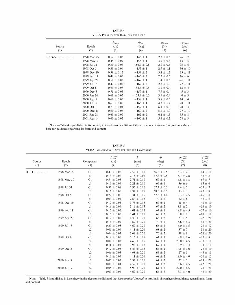
TABLE 4

VLBA Polarization Data for the Core

Source

(1)

Epoch

(2)

I7 mm

(Jy)

(3)

�jet

(deg)

(4)

m7 mm

(%)

(5)

�7 mm

(deg)

(6)

3C 66A....................... 1998 Mar 25 0.52 � 0.05 �146 � 1 2.3 � 0.6 26 � 7

1998 May 30 0.45 � 0.07 �155 � 1 3.7 � 0.8 13 � 5

1998 Jul 31 0.30 � 0.03 �150.7 � 0.5 2.9 � 0.6 35 � 6

1998 Oct 5 0.31 � 0.04 �155 � 1 2.7 � 1.1 36 � 10

1998 Dec 10 0.39 � 0.12 �159 � 2 3.1 � 1.3 13 � 11

1999 Feb 11 0.48 � 0.05 �146 � 2 2.2 � 0.5 16 � 6

1999 Apr 29 0.50 � 0.03 �167 � 1 1.4 � 0.6 �6 � 11

1999 Jul 18 0.47 � 0.02 �162 � 2 2.3 � 1.0 27 � 11

1999 Oct 6 0.69 � 0.03 �154.4 � 0.5 3.2 � 0.4 18 � 4

1999 Dec 5 0.75 � 0.03 �159 � 1 7.7 � 0.4 5 � 3

2000 Jan 24 0.61 � 0.05 �155.4 � 0.5 3.9 � 0.4 0 � 3

2000 Apr 5 0.60 � 0.05 �158 � 1 3.8 � 0.5 14 � 4

2000 Jul 17 0.63 � 0.08 �163 � 1 4.3 � 1.7 28 � 11

2000 Oct 1 0.73 � 0.04 �159 � 1 6.1 � 0.3 28 � 3

2000 Dec 11 0.60 � 0.06 �160 � 2 5.7 � 1.0 27 � 10

2001 Jan 28 0.63 � 0.07 �162 � 2 6.1 � 1.5 35 � 8

2001 Apr 14 0.60 � 0.05 �160 � 1 5.4 � 0.3 28 � 3

Note.—Table 4 is published in its entirety in the electronic edition of the Astronomical Journal. A portion is shownhere for guidance regarding its form and content.

TABLE 5

VLBA Polarization Data for the Jet Component

Source

(1)

Epoch

(2)

Component

(3)

Icomp7 mm

(Jy)

(4)

R

(mas)

(5)

�

(deg)

(6)

mcomp7 mm

(%)

(7)

�comp7 mm

(deg)

(8)

3C 111.................. 1998 Mar 25 C1 0.43 � 0.08 2.50 � 0.10 66.8 � 0.5 6.3 � 2.1 �44 � 10

c1 0.14 � 0.06 2.15 � 0.08 67.6 � 0.5 15.7 � 2.8 �43 � 8

1998 May 30 C1 0.54 � 0.08 2.71 � 0.10 67 � 1 6.8 � 1.8 �67 � 7

c1 0.10 � 0.04 2.21 � 0.10 69 � 1 36 � 6 �65 � 6

1998 Jul 31 C1 0.32 � 0.08 2.93 � 0.10 67.7 � 0.5 9.4 � 2.1 �55 � 7

c1 0.16 � 0.05 2.34 � 0.15 68.5 � 0.5 13 � 3 �47 � 8

1998 Oct 5 C1 0.22 � 0.06 3.31 � 0.15 67.5 � 1.0 9.3 � 2.5 �45 � 8

c1 0.09 � 0.04 2.64 � 0.15 70 � 2 32 � 6 �45 � 6

1998 Dec 10 C1 0.17 � 0.05 3.73 � 0.15 67 � 1 15 � 4 �40 � 10

c1 0.16 � 0.04 3.16 � 0.15 69 � 2 8.8 � 2.1 �54 � 10

1999 Feb 11 C1 0.17 � 0.05 4.01 � 0.15 67 � 1 18.8 � 4.5 �57 � 10

c1 0.15 � 0.05 3.41 � 0.15 69 � 2 8.8 � 2.1 �60 � 10

1999 Apr 29 C1 0.12 � 0.05 4.33 � 0.20 66 � 2 21 � 5 �22 � 20

c1 0.16 � 0.07 3.62 � 0.20 70 � 2 15.6 � 4.3 �41 � 20

1999 Jul 18 C1 0.20 � 0.05 4.69 � 0.20 66 � 2 6.0 � 1.5 �29 � 12

c2 0.06 � 0.04 4.11 � 0.20 68 � 2 37 � 7 �31 � 20

c1 0.04 � 0.03 3.69 � 0.20 70 � 2 38 � 8 �26 � 20

1999 Oct 6 C1 0.19 � 0.05 5.16 � 0.15 64 � 1 8.9 � 1.6 �27 � 8

c2 0.07 � 0.03 4.63 � 0.15 67 � 1 20.0 � 4.5 �37 � 10

c1 0.11 � 0.04 3.90 � 0.15 69 � 1 10.9 � 3.4 �31 � 10

1999 Dec 5 C1 0.12 � 0.05 5.46 � 0.15 64 � 2 14.5 � 3.6 �28 � 10

c2 0.06 � 0.03 4.98 � 0.20 66 � 2 27 � 5 �43 � 15

c1 0.10 � 0.04 4.11 � 0.20 68 � 2 18.0 � 4.0 �50 � 15

2000 Apr 5 c2 0.05 � 0.03 5.37 � 0.20 64 � 2 22 � 5 �23 � 20

c1 0.09 � 0.04 4.52 � 0.20 64 � 2 15.6 � 4.5 �42 � 20

2000 Jul 17 c2 0.05 � 0.03 5.90 � 0.20 64 � 2 22.0 � 4.5 �23 � 20

c1 0.09 � 0.04 4.69 � 0.20 64 � 2 13.3 � 4.0 �42 � 20

Note.—Table 5 is published in its entirety in the electronic edition of the Astronomical Journal. A portion is shown here for guidance regarding its formand content.

of linear polarizationmcomp7 mm, and (8) polarization position angle

�comp7 mm in the component. Values of the degree of polarization in

both tables are corrected for statistical bias.

3. OBSERVED CHARACTERISTICS OF POLARIZATION

Tables 1Y4 show that the linear polarization for all objects atmost wavelengths varies significantly both in degree and positionangle. Figure 1 represents the relationship between the degree ofpolarization at optical, 1 mm, and 3 mm wavelengths from thewhole source with respect to the degree of polarization measuredin the VLBI core at 7 mm. The data plotted in Figure 1 correspondto the closest observations obtained at opticalY7 mm, 1Y7 mm,and 3Y7 mmwavelengths for each source. These measurementsare simultaneous within 1Y3 days. There is a statistically signifi-cant correlation at a significance level � ¼ 0:0514 between frac-tional polarization in the VLBI core and degree of polarization atshort wavelengths. The optical polarization maintains the stron-gest connection to the polarization in the VLBI core (r ¼ 0:87,where r is the linear coefficient of correlation). This result con-firms the strong correlation between the polarization level of theradio core at 7mmand overall optical polarization found by Lister& Smith (2000). Their sample included quasars with both highand low optical polarization. However, it raises the question ofwhy the optical polarization shows a better connection to thepolarization in the VLBI core than does the polarization at 1 mm.

3.1. Polarization Variability

We have computed the fractional polarization variability indexV

pk at each frequency using the definition employed byAller et al.

(2003b),

Vp

k ¼(mmax

k � �mmaxk

)� (mmink þ �mmin

k)

(mmaxk � �mmax

k) þ (mmin

k þ �mmink); ð1Þ

where mmaxk and mmin

k are, respectively, the maximum and mini-mum fractional polarization measured over all epochs at wave-length k, and �mmax and �mmin are the corresponding uncertainties.This approach is especially justified in our case, since all objectswere observed over the same period of time, although the timeintervals are different at different wavelengths (�2 yr in the op-tical,�1 yr at 3 mm, and�3 yr at 1 and 7 mm). Note that equa-tion (1) can produce a negative variability index if the degree ofpolarization or maximum change in polarization do not exceedthe uncertainties in the measurements. In this case the data fail toreveal polarization variability, and we setV p ¼ 0.We introducethe polarization position angle variability index, V a

k :

V ak ¼

j��kj �ffiffiffiffiffiffiffiffiffiffiffiffiffiffiffiffiffiffiffi�2�1kþ �2

�2k

q

90; ð2Þ

where ��k is the observed range of polarization direction and��1

kand ��2

kare the uncertainties in the two values of EVPAs

that define the range. We treat the 180�ambiguities in EVPAs

such that��k cannot exceed 90�. As in the case of V p, if V a � 0

then we set V a ¼ 0 and conclude that the observations were un-able to measure variability in the polarization position angle.

Figure 2 shows the relationship between the polarization andposition angle variability indices in the VLBI core and at shortwavelengths. A statistically significant correlation occurs both be-tween V

popt and V

p7 mm and between V a

opt and V a7 mm (r ¼ 0:62 and

0.78, respectively). This result indicates that changes in the or-dering of magnetic fields in the optical region and VLBI coreare correlated, which suggests that the polarization variability hasthe same origin at the two wave bands. The correlation betweenthe values at 3 mm and in the VLBI core might be affected by theregion of the jet lying somewhat outside the VLBI core that con-tributes significantly to the 3 mm polarized emission. There isno correlation between variability indices at 1 mm and in theVLBI core.

3.2. A Polarization-based Classification Scheme

Weuse the polarization variability indices to classify the sourcesin our sample with respect to their polarization properties. Thisclassification scheme differs somewhat from the classical separa-tion of AGNs into radio galaxies, quasars, and BL Lac objects,which we have used to discuss kinematics in the parsec-scale jets(J05). The new categorization reveals significant differences in

Fig. 1.—Degree of polarization at optical, 1 mm, and 3mmwavelengths fromthe whole source vs. degree of polarization measured in the VLBI core at 7 mmfor the most nearly simultaneous pair of observations for each source. The linearcoefficient of correlation, r, is given in each panel. Symbols denote quasars (opencircles), BL Lac objects ( filled circles), and radio galaxies (triangles).

14 Throughout the paperwe calculate coefficients of linear correlation and usethe method of Bowker & Lieberman (1972) for testing the significance of thesecoefficients. The hypothesis that there is no correlation between two variables,r ¼ 0, can be rejected at a significance level � if t ¼ jr/(1� r 2)1

=2j(N � 2)1=2 �

t�=2;N�2; where t�=2;N�2 is the percentage point of the t-distribution for N � 2degrees of freedom and N is the number of observations.


the polarization properties (see x 7) among the introduced groupsthat would be diluted in the traditional scheme.

Figure 3 shows that the fractional polarization and polarizationposition angle variability indices in the 7 mm core are stronglycorrelated (r ¼ 0:83) in a way that produces a clear separation ofthe sources into three groups: LVP (low variability of polarizationin the radio core, V

p7 mm � 0:2, V a

7 mm � 0:4), IVP (intermediatevariability of polarization, 0:2 < V

p7 mm � 0:6, 0:2 < V a

7 mm �0:7), and HVP (high variability of polarization in the radio core,V

p7 mm > 0:6, V a

7 mm > 0:7). (We note, however, that low electricvector variability indices in the LVP group could result from largeuncertainties in EVPAs connectedwith low fractional polarization.)

The LVP group includes the two radio galaxies 3C 111 and3C 120 plus the low optically polarized quasar 3C 273. All threesources display low fractional polarization in the optical bandand in the 7 mm core. However, in the quasar 3C 273 the opticalsynchrotron emission is known to be variable and to have m >10% if dilution from essentially unpolarized nonsynchrotroncomponents such as the big blue bump is taken into account(Impey et al. 1989). All three LVP sources are highly polarizedand variable at 1 mm, and the fractional polarization of 3C 273at 3 mm might be as high as 4%.

The IVP group consists of four (out of five) BL Lac objectsand two highly optically polarized quasars, 3C 279 and 3C 345.This group, therefore, includes extremely highly polarized blazars,whose polarization in the optical and at 1 mm can exceed 30%and whose polarization at 3 mm and in the VLBI core does notdrop below 2%Y3%. Note that Nartallo et al. (1998) have foundno differences in polarization properties of BL Lac objects andcompact flat-spectrum quasars at short millimeter and submil-limeter wavelengths.

The majority of the quasars (five out of eight) and one BL Lacobject, OJ 287, form the HVP group. The linear polarization ofthe VLBI core in these sources can be very low, i.e., at the noiselevel, or as high as �5%. The polarization variability indices,V p, at 3 mm, 1 mm, and optical wavelengths are similar to those

for the IVP group, although V a indices indicate more dramaticpolarization position angle variability at all wavelengths. We didnot observe high polarization at short millimeter wavelengths(m3 mm � 10% andm1 mm � 15%) as in the IVP group, althoughvery high optical polarization (mopt � 20%) might occur in thesesources as often as in IVP sources (Hagen-Thorn 1980).

Figure 4 presents the distributions of fractional polarizationfor all of our measurements, separated according to the variabilitygroups. Comparison of the distributions shows that (1) the peakof the distribution in the IVP group occurs at a higher percent-age polarization than for the other two groups, independent ofwavelength, and (2) for a given variability group, the peak ofthe distribution shifts to higher fractional polarization at shorterwavelengths except for the LVP sources, where the optical po-larization is similar to the polarization in the VLBI core.

4. TOTAL AND POLARIZED FLUX DENSITY SPECTRA

We have constructed single-epoch total and polarized fluxdensity spectra based onmeasurements at different wavelengthsobtained within 2 weeks of each other (except 1803+784 and1823+568, where, at best, there is nearly a month between ob-servations at differentwavelengths).We have corrected the opticalflux densities shown in Table 1 for Galactic extinction using val-ues of Ak compiled by the NASA/IPAC Extragalactic Database.The total flux densities at 7 mm are corrected for possible missingflux density in the VLBA images using single-dish observationsas described in J05. The measurements at 7 mm include the coreand components within the 1% contours of the peak total inten-sity at a given epoch (J05), Ijet ¼ I core þ

Pi I

compi . The polarized

flux density at 7 mm is integrated over the same VLBA image.Therefore, I

pjet ¼ (Q2

jet þU2jet )

1=2; Qjet ¼QcoreþP

i Qcompi ;Ujet ¼

U core þP

i Ucompi

; mjet ¼ Ipjet/Ijet; and �jet ¼ 0:5 tan�1(Ujet /Qjet),

where I core,Qcore, andU core are the Stokes parameters of the core,and I

compi ,Q

compi , andU

compi are the Stokes parameters of a given

polarized jet component. Figure 5 presents the total and polarizedspectral energy distributions (SEDs), while Table 6 lists the spec-tral indices�mm (based on total flux densities at the threemillimeter

Fig. 2.—Left : Dependence on polarization variability index at optical, 1 mm,and 3 mm wavelengths and polarization variability index in the VLBI core at7mm.Right : Dependence on polarization position angle variability index at optical,1 mm, and 3 mm wavelengths and polarization position angle variability indexin the VLBI core at 7 mm. The symbols are the same as in Fig. 1.

Fig. 3.—Connection between polarization and position angle variabilityindices in the VLBI core at 7 mm. Symbols denote the quasars (open circles),BL Lac objects ( filled circles), and radio galaxies (triangles).


wavelengths) and �opt=1 mm, where S� / �� . We calculate thespectral indices � p

mm and � popt=1 mm using the corresponding po-

larized flux densities, S p� / ��p

.Table 6 shows that the total flux density spectra at millimeter

wavelengths are flat independent of the type of source, with themajority of spectral indices having j�mmj< 0:5. This confirmsthat the millimeter-wave emission is partially optically thick.The optical-millimeter spectra of the HVP sources are steep,with �opt=1 mm � 1, while the LVP sources possess much flatteroptical to 1 mm spectra. In the IVP group �opt=1 mm depends onwhether the source is a quasar (�opt=1 mm � 1) or a BL Lac ob-ject (�opt=1 mm � 0.5). The polarized flux density spectra at mil-limeter wavelengths are flat or inverted, which indicates anincrease of polarized emissionwith frequency at millimeter wave-lengths. Figure 6 reveals a strong correlation between � p

opt=1 mmand �opt=1 mm (r ¼ 0:92). However, two sources from the LVPgroup (3C 120 and 3C 273) deviate greatly from the depen-dence � p

opt=1 mm ¼ �opt=1 mm (Fig. 6, solid line), with a signifi-cantly steeper polarized flux density spectral index than for thetotal flux density. This suggests that at least two emission com-ponents are present in the optical region, one of which is un-polarized. Impey et al. (1989) found an increase in the degreeof polarization and higher variability of the Stokes parameters in3C 273 at longer optical wavelengths. Such behavior is expectedif the optical emission consists of a variable synchrotron com-ponent plus a relatively static blue unpolarized continuum source,such as the big blue bump. The decomposition of the optical syn-

chrotron spectrum from other optical emission sources is readilyseen in the spectropolarimetry of 3C 273 (Smith et al. 1993). Inthe case of 3C 120, the strong dilution of the optical synchrotronpolarization is likely caused by host galaxy starlight includedwithin the measurement aperture.In themajority of theHVP and IVP sources, the spectral indices

�popt=1 mm and�opt=1 mm are similar to each other. This suggests that

a single synchrotron component is responsible for the total fluxand polarized continuum from millimeter to optical wavelengths.However, three of the HVP sources (0420�014, 1510�089, and3C 454.3) have a slightly steeper polarized flux density spectrumrelative to the total flux density spectrum (this was found previ-ously aswell by Smith et al. 1988). In the IVP sources the oppositetrend prevails, except for BL Lac. A steeper polarized spectrum inthe quasars indicates the possible presence of a nonsynchrotroncomponent, such as that observed for 3C 273, although its con-tribution to the total flux should be P10% relative to the syn-chrotron emission. A flatter polarized spectrum likely rules outany significant contribution by a nonsynchrotron component,although two (or more) synchrotron components might coexistin the IVP sources. For BL Lac, contribution to the optical fluxfrom the host galaxy might help to explain why the � p

opt=1 mm isslightly steeper than the total flux spectral index.

5. FARADAY ROTATION IN THE INNER JET

Figure 5 presents measurements of the polarization angle� atdifferent frequencies obtained within 2 weeks of each other and

Fig. 4.—Distributions of degree of linear polarization in the IVP (left ), HVP (middle), and LVP (right ) variability groups at optical, 1 mm, and 3 mm wavelengthsand in the VLBI core at 7 mm.


shows that the direction of millimeter-wave polarization rotateswith wavelength. In the HVP and IVP sources the EVPA at 7 mmdisplayed in the figure corresponds to that of the VLBI core only,while in the LVP sources it corresponds to�jet , as described in x 4.We attribute this rotation to Faraday rotation by a foregroundscreen close to the VLBI core (Zavala & Taylor 2004; Attridgeet al. 2005). We define the rotation measure (RM) by assuming

that at 1 mm we see the unrotated direction of the polarizationand that the emission from 1 to 7 mm propagates through thesame screen.

5.1. Faraday Rotation in the HVP and IVP Sources

Figure 7 shows the result of fitting the dependence of the po-larization position angle onwavelength by a Faraday rotation law:

Fig. 5.—Total (circles) and polarized (triangles) flux density spectra and polarization position angle (crosses) measurements from optical to 7 mm wavelengths.


� ¼ �1 mm þ RMk2. For 0420�014 our program does not con-tain simultaneous observations at three wavelengths necessaryto estimate RM. We have supplemented our data by observationsobtained with the VLBA at 7 mm and 1.3 cm in the programBG073 (seeGomez et al. 2000), forwhich 0420�014 and 3C454.3were used as calibrators. For 0420�014 we use our polarizationmeasurement at 1 mm on 1998 December 13 and EVPAs inthe 7 mm and 1.3 cm core on 1998 December 3 from BG073.The EVPA at 7 mm is consistent with �7 mm at epoch 1998December 11 from our program. For 3C 454.3 and BL Lac weuse observations different from those plotted in Figure 5. For3C 454.3 we use observations at 1 and 3 mm from our program(2000 June 6 and 8, respectively) and 7 mm VLBA observa-tions on 2000 June 9 (BG073). These observations are closerto each other than the measurements presented in Figure 5 (2000

November 29YDecember 11) and less affected by the variabilityof bright component B6 seen on the images (J05). We have in-cluded the contribution of the component in the polarization at7 mm because B6 is brighter and more highly polarized than thecore and located within 0.2 mas of the core. For BL Lac we useobservations carried out over the period 2001 January 17Y28 inorder to have simultaneous measurements at 3 mm wavelengths.Table 7 gives the values of correction for EVPAs at 3 and 7mm

along with the intrinsic rotation measure for each object, RM0 ¼RM(1þ z)2. Some of the RM values have large uncertaintiesthat might be attributed to several problems that our observationspossess. First, the observations are not completely simultaneous,whereas the polarization position angle can sometimes have shorttimescales of variability even at 7 mm (D’Arcangelo et al. 2007).Second, the polarization position angles at 7 mm correspond tothose of the VLBI core only, while the EVPAs at 1 and at 3mmarefrom the whole source. Although we have tested that, at epochsused for estimates of the rotation measure, jet components con-tribute little to the polarization of the core (except 3C 454.3), theircontribution to the polarized flux at 1 and 3 mm is unknown.Third, the structure of the magnetic field in the 7 mm core and inthe regions emitting at shorter millimeter wavelengths, especiallyat 1 mm, might be different. Therefore, the observed rotationcould be an intrinsic property of the magnetic field structure.To test that the derived rotation measures are reliable, we

construct the distributions of ��3Y7 ¼ j�3 mm � �7 mmj for allpairs of observations simultaneous within 2 weeks for �k beforeand after RM correction (Fig. 8). Note that the distributions do notinclude the observations used to calculate the rotation measures.This avoids the bias that these observations would introduce tothe distributions. Ideally, the EVPAs after RM correction shouldalign within 10

�Y20�, which corresponds to the uncertainties ofour measurements. This is a feature of both distributions (un-corrected and corrected) for the IVP sources, reflecting the factthat in the IVP sources the uncertainties of EVPAs are com-parable to the RM correction values. However, EVPAs correctedfor RM exhibit a slightly better alignment than ��3Y7 before thecorrection, as is expected if the EVPA rotation is caused by aFaraday screen. In the HVP sources the RM correction signif-icantly improves alignment between �3 mm and �7 mm; 69% ofuncorrected values of ��3Y7 exceed 20�, while only 44% of

TABLE 6

Total and Polarized Flux Spectral Indices

Source

(1)

Group

(2)

�opt=1 mm

(3)

� p

opt=1 mm

(4)

�mm

(5)

� pmm

(6)

3C 111........................ LVP 0.55 � 0.02 0.60 � 0.04 0.52 � 0.05 0.15 � 0.20

3C 120 ....................... LVP 0.56 � 0.02 1.03 � 0.05 0.47 � 0.02 �0.28 � 0.34

3C 273 ....................... LVP 0.66 � 0.01 1.04 � 0.07 0.64 � 0.16 0.51 � 0.27

3C 66A....................... IVP 0.60 � 0.01 0.50 � 0.02 0.16 � 0.09 �0.11 � 0.21

3C 279 ....................... IVP 1.19 � 0.01 1.01 � 0.04 0.08 � 0.06 �0.13 � 0.03

3C 345 ....................... IVP 1.06 � 0.01 0.95 � 0.01 0.53 � 0.06 0.06 � 0.36

1803+784 ................... IVP . . . . . . 0.28 � 0.17 0.19 � 0.15

1823+568 ................... IVP . . . . . . 0.27 � 0.17 0.12 � 0.23

BL Lac ....................... IVP 0.50 � 0.01 0.54 � 0.02 0.15 � 0.04 0.08 � 0.09

0420�014 .................. HVP 1.00 � 0.01 0.86 � 0.01 0.25 � 0.03 0.11 � 0.05

0528+134 ................... HVP 0.96 � 0.02 0.98 � 0.05 0.48 � 0.03 �0.32 � 0.26

OJ 287........................ HVP 0.90 � 0.01 0.80 � 0.01 0.24 � 0.06 �0.25 � 0.12

1510�089 .................. HVP 0.90 � 0.01 1.13 � 0.04 0.68 � 0.07 �0.44 � 0.17

CTA 102 .................... HVP 1.00 � 0.02 0.97 � 0.06 0.37 � 0.20 0.11 � 0.12

3C 454.3 .................... HVP 0.97 � 0.01 1.05 � 0.02 0.40 � 0.13 �0.11 � 0.32

Notes.—Uncertainties for �opt=1 mm are determined from uncertainties of flux measurements; uncertainties for �mm

are based on consistency between different wavelengths.

Fig. 6.—Dependence between polarized and total flux spectral indices cal-culated between the optical and 1 mm wavelengths (open circles: HVP sources;filled circles: IVP sources; triangles: LVP sources).


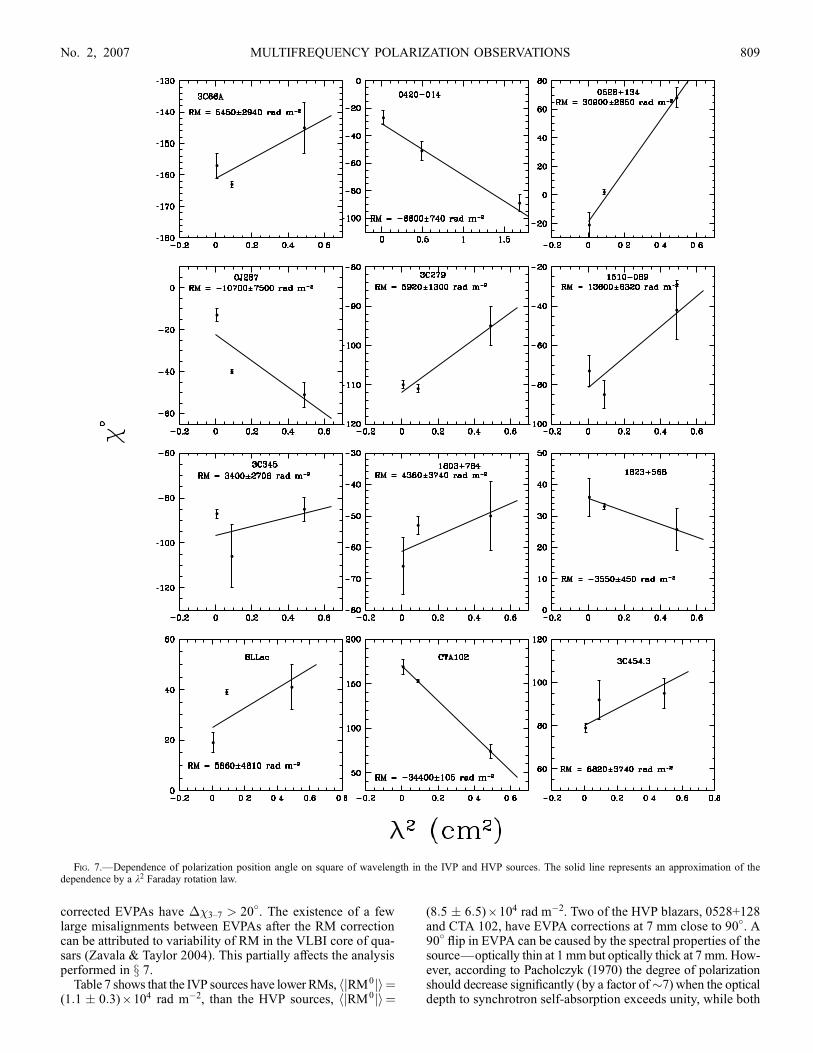
corrected EVPAs have ��3Y7 > 20�. The existence of a fewlarge misalignments between EVPAs after the RM correctioncan be attributed to variability of RM in the VLBI core of qua-sars (Zavala & Taylor 2004). This partially affects the analysisperformed in x 7.

Table 7 shows that the IVP sources have lower RMs, hjRM0ji ¼(1:1 � 0:3) ; 104 rad m�2, than the HVP sources, hjRM0ji ¼

(8:5 � 6:5) ; 104 rad m�2. Two of the HVP blazars, 0528+128and CTA 102, have EVPA corrections at 7 mm close to 90

�. A

90� flip in EVPA can be caused by the spectral properties of thesource—optically thin at 1 mm but optically thick at 7 mm. How-ever, according to Pacholczyk (1970) the degree of polarizationshould decrease significantly (by a factor of�7) when the opticaldepth to synchrotron self-absorption exceeds unity, while both

Fig. 7.—Dependence of polarization position angle on square of wavelength in the IVP and HVP sources. The solid line represents an approximation of thedependence by a k2 Faraday rotation law.


TABLE 7

Rotation Measures

Source

(1)

z

(2)

Group

(3)

��3 mm

(deg)

(4)

��7 mm

(deg)

(5)

RM043 GHz

(103 rad m�2)

(6)

RM015 GHz

(103 rad m�2)

(7)

RM08 GHz

(103 rad m�2)

(8)

a

(9)

3C 66A.......................... 0.444 IVP �3 �16 12 � 6 . . . . . . . . .

3C 279 .......................... 0.538 IVP �3 �16 14 � 2 �5.7 (2) 3.1 (1) 0.92 � 0.04

3C 345 .......................... 0.595 IVP �2 �9 11 � 7 . . . �0.33� (3) 1.6

1803+784 ...................... 0.68 IVP �3 �16 12 � 9 . . . 0.56 (1) 1.8

1823+568 ...................... 0.664 IVP 1 7 �10 � 1 1.1 (2) 0.36 (1) 1.81 � 0.02

BL Lac .......................... 0.069 IVP �3 �16 6.7 � 5.5 7.0 (2) 0.42 (1) 1.5 � 1.2

0420�014 ..................... 0.915 HVP 4 19 �24 � 3 . . . . . . . . .

0528+134 ...................... 2.06 HVP �16 �87 280 � 30 . . . 1.5 (1) 3.1

OJ 287........................... 0.306 HVP 6 30 �19 � 11 . . . . . . . . .

1510�089 ..................... 0.361 HVP �7 �38 26 � 10 . . . . . . . . .

CTA 102 ....................... 1.037 HVP 18 97 �140 � 40 . . . �4.2� (4) 1.6

3C 454.3 ....................... 0.859 HVP �4 �19 24 � 13 . . . 9.0 (1) 1.8

Notes.—Col. (1): Name of the source. Col. (2): Redshift. Col. (3): Polarization variability group. Col. (4): RM correction at 3 mm. Col. (5): RM correction at 7 mm.Col. (6): Intrinsic RM obtained in the 43 GHz core. Col. (7): Intrinsic RM obtained in the 15 GHz core. Col. (8): Intrinsic RM obtained in the 8 GHz core. An asteriskdenotes intrinsic RM obtained in the core at 5 GHz instead of 8 GHz; numbers in parentheses denote references for RM0 measured at low frequencies (1: Zavala & Taylor2003; 2: Gabuzda et al. 2006; 3: Taylor 1998; 4: Taylor 2000). Col. (9): The exponent in the relation RM / d�a.

Fig. 8.—Distributions of offsets between EVPAs at 3 mm and in the 7 mm core before the RM correction (left ) and after the RM correction (right ). The distributionsdo not include the observations used to calculate the RM.

quasars show only amoderate decrease of polarization from 1 to7 mm at the epochs used to calculate RM (m1 mm ¼ 4:7% �1:6% andm7 mm¼1:8% � 0:5% for 0528+134;m1 mm ¼ 6:5% �1:9% and m7 mm ¼ 4:0% � 0:7%% for CTA 102).

In a sample of 40 AGNs Zavala & Taylor (2004) have de-termined RMs using VLBI images at 8Y15 GHz that are lowerthan we derive at millimeter wavelengths. The authors suggestthat an external screen ‘‘in close proximity to the jet’’ is the mostpromising candidate for the source of the Faraday rotation. In thiscontext, lower RMs obtained in the VLBI core at longer wave-lengths might reflect a strong decrease in thickness of the screenwith distance from the central engine. This is expected becausethe location of the core shifts with wavelength owing to opticaldepth effects.We assume a decreasing gradient in electron densityof the screen, described by a power law,Ne / d�a, where d is thedistance from the central engine. The RM depends on the densityandmagnetic field parallel to the line of sight, Bk, integrated alongthe path through the screen to the observer: RM /

RNeBkdl. In

the absence of a velocity gradient across the jet, the magnetic fieldalong the jet scales as Bz / d�2, and the magnetic field trans-verse to the jet scales as B� / d�1 (Begelman et al. 1984). If theFaraday screen is at least mildly relativistic and has a helicalfield (Gabuzda 2006), B� provides the main contribution to themagnetic field component along the line of sight; therefore,Bk / d�1. This leads to jRMj / d�a under the approximation thatl / d. The location of the core from the central engine depends onthe frequency of the observation � as derived, for example, inLobanov (1998): dcore; � ¼ (Bkb

1 F /�)1=kr ;whereB1 is themagnetic

field at distance 1 pc from the central engine, F is a function ofthe redshift and parameters depending on the jet geometry andrelativistic electron energy distribution, and the equipartion val-ue kr ¼ 1. For a source with a flat millimeter-wave spectrumdcore; � / ��1, which yields the dependence of the RM observedin the core on the frequency of observation as jRMcore;� j / � a.Therefore, values of RM obtained with different sets of frequen-cies should produce an estimate of the parameter a. We assumethat the RM0 derived from polarization observations of the coreat frequencies �1, �2, and �3, where �3 is the lowest one, yieldsthe intrinsic RM at the location dcore;�3 .

Table 7 contains the published RMs obtained in the VLBIcore at wavelengths longer than 7 mm, RM0

15 GHz and RM08 GHz,

and derived values of a. For sources with RM0 available at morethan twowavelengths,a is calculated using a least-squaresmethod.Table 7 does not show any difference in the values of a betweenthe HVP and IVP sources. The average hai ¼ 1:8 � 0:5 is sim-ilar to the value a ¼ 2 expected for outflow in a spherical orconical wind. This implies that an outflowing sheath wrappedaround a conically expanding jet is a reasonable model forthe foreground screen, consistent with the finding of Zavala& Taylor (2004). The sheath can result from a mildly relativ-istic outer wind that emanates from the accretion disk and con-fines the inner relativistic jet (Gracia et al. 2005). According tothe RM0 values in Table 7, the thickness of the sheath is higherin the HVP sources with respect to the IVP sources, a situationthat should assist in stronger confinement of the jet of HVPblazars. The latter may help to explain the finding by J05 thatthe jet opening angles for quasars are smaller than for BL Lacobjects.

We have corrected the values of �3 mm and �7 mm in the HVPand IVP sources for Faraday rotation by applying the correc-tions listed in Table 7 to the EVPAs given in Tables 3 and 4.The adjusted values of the EVPAs are used in the subsequentanalysis.

5.2. Faraday Rotation in the LVP Sources

In the LVP sources, the core at 7 mm is unpolarized; hence,the polarization position angle of the inner jet is defined by thepolarization of VLBI components within a few milliarcsecondsof the core. For the epochs shown in Figure 5 these are com-ponents C1 and c1 at �4 mas in 3C 111, components t and u at1Y2 mas in 3C 120, and component B2 at 1 mas in 3C 273.Figure 9 shows the k2 dependence of � in 3C 273, which yieldsa high RM, RM ¼ (1:6 � 0:5) ; 104 rad m�2. The value is con-sistent with the high RM obtained for component Q6/W6 fromthe 43/86 GHz images by Attridge et al. (2005), RM ¼ 2:1 ;104 rad m�2. However, a significant decrease in the density ofthe Faraday screen with distance from the core discussed aboveexplains the good alignment between the EVPA at 1 mm and�jet when components are seen farther downstream. This occursfor 3C 111 and 3C 120: in 3C 111 �1 mm ¼ �54� � 6� and�jet ¼�58

� � 10�, in 3C 120�1 mm ¼�38

� � 4�and�jet ¼ �35

� � 6�.

The implication is that the magnetic fields in the 1 mm emissionregion have the same orientation as that in the jet features a fewmilliarcseconds from the core. Very low polarization in the VLBIcore at 7 mm, the high RM obtained close to the core in 3C 273,and consistency between the direction of polarization in the innerjet and at 1 mm in 3C 111 and 3C 120, all suggest that in the LVPsources the 1 and 3mm cores have low polarization as well. Thelow polarization of the core could be the result of either fine-scale turbulence or depolarization by a very thick, inhomogeneousforeground screen with RM > 5 ; 105 rad m�2, as suggested byAttridge et al. (2005).

The EVPAs of the LVP sources are not corrected for RMowingto the complexities discussed above. We use the simplificationthat, when strong polarized components are detected, they havealready left the high-RM zone.

6. CORRELATION ANALYSIS

6.1. Comparison of Polarization at Different Wavelengths

Wehave calculated linear coefficients of correlation f p betweenthe polarized flux densities in the core at 7 mm and overall

Fig. 9.—Dependence of polarization position angle on square of wavelengthin 3C 273. The solid line represents an approximation of the dependence by a k2

Faraday rotation law.

MULTIFREQUENCY POLARIZATION OBSERVATIONS 811

polarized flux density measurements at (1) optical, fpoY7, (2) 1 mm,

fp1Y7, and (3) 3 mm, f

p3Y7. These apply to sources having data

from at least three essentially simultaneous observations at twowavelengths. (Here we consider the observation at two wave-lengths ‘‘simultaneous’’ if they are obtained within 2 weeks ofeach other.)We do the same for the correlation coefficients rm ofthe the degree of polarization in the core at 7 mm and the overallfractional polarization in each of the other wave bands, using thesame subscript designations. For some sources several measure-ments have been carried out at high frequencies within 2 weeks ofa few VLBA epochs. In these cases, we use only the observationthat is nearest to the correspondingVLBAepoch. Table 8 containscoefficients of correlation f

poY7, f

p1Y7, and f

p3Y7 (cols. [2]Y[4]) and

rmoY7, rm1Y7, and rm3Y7 (cols. [5]Y[7]). The number of points par-

ticipating in the computation is indicated in parentheses. Thecoefficients of correlation that are significant at a level � ¼ 0:1are indicated with asterisks.

The correlation coefficients between optical polarization andpolarization in the core at 7 mm correspond to neither positivenor inverse correlation despite otherwise similar overall polar-ization characteristics (see x 3). Blazars are known to have veryshort timescales of polarization variability at optical wavelengths(<1 day, Hagen-Thorn 1980; Moore et al. 1987; Mead et al.1990). Because of this, we suspect that the lack of exact simul-taneity and the small number of observations affect the correlationanalysis in the optical band.

The statistically significant coefficients of correlation listedin Table 8 indicate a strong positive correlation either betweenthe polarized flux in the core at 7 mm and overall source at 1 and3 mm, or between the fractional polarization in the core and atshorter millimeter wavelengths. However, the number of sourceswith such behavior corresponds to 25% and 45% for the 1Y7 mmand 3Y7 mm data, respectively. The absence of statisticallymeaningful correlations for other sources might be explained byeither small-number statistics, e.g., for 0420�014 or 1510�089,or by contributions from jet components different from the core tothe polarized flux at 1 and 3 mm. Table 9 gives the coefficients ofcorrelation of the sources for which inclusion of the jet compo-nents (see x 4) changes the significance of the correlation. Table 9shows that including highly polarized components within a few

milliarcseconds from the core dramatically improves the corre-lation in (1) all the LVP sources, (2) two of the HVP sources(CTA 102 and 3C 454.3), and (3) none of the IVP sources. For3C 279 the correlation coefficient between the 7 and 1 mm polar-ization increases (rm1Y7 ¼ 0:51) but does not change its signifi-cance substantially.

6.2. PolarizationYTotal Flux Connectionat Different Wavelengths

We have computed coefficients of correlation between thedegree of polarization and total flux density, rk (listed inTable 10),and between the polarized and total flux densities, fk (given inTable 11). The coefficients are calculated for each source that hasthree or more simultaneous measurements of the two quantities atwavelength k (in this case the observations are completely simul-taneous). Since the JCMT observations were performed at 1.35and 0.85 mm, we have adjusted flux densities and fractional po-larization at 0.85 mm to 1.35 mm using the spectral indices �mm

and � pmm provided in Table 6. The data at 1 mm are supplemented

by the measurements obtained by Nartallo et al. (1998) at 1.1 mmfor sources common to both samples: 0420�014, 0528+134,OJ 287, 3C 273, 3C 279, 3C 345, 1823+568, BL Lac, and3C 454.3. Coefficients of correlation r7 mm and f7 mm correspondto the VLBI core only.

TABLE 8

Correlation Coefficients between Polarization in the Core at 7 mm and Overall Polarization

at Optical, 1 mm, and 3 mm Wavelengths

Source

(1)

fpoY7

(2)

fp1Y7

(3)

fp3Y7

(4)

rmoY7(5)

rm1Y7(6)

rm3Y7(7)

3C 66A....................... 0.81 (4)� 0.22 (8) 0.81 (3) 0.97 (4)� 0.21 (8) 0.81 (3)

3C 111........................ . . . (1) . . . (0) . . . (2) . . . (0) . . . (0) . . . (0)

0420�014 .................. 0.67 (4) 0.94 (5)� . . . (1) 0.72 (5) 0.55 (4) . . . (1)3C 120 ....................... . . . (1) . . . (2) . . . (1) . . . (1) . . . (2) . . .(1)

0528+134 ................... . . . (1) �0.17 (8) �0.38 (3) . . . (1) �0.49 (8) 0.14 (3)

OJ 287........................ 0.33 (6) 0.78 (7)� �0.11 (5) 0.30 (6) 0.68 (7)� 0.25 (5)

3C 273 ....................... . . . (1) . . . (2) . . . (2) . . . (1) . . . (2) . . . (2)

3C 279 ....................... 0.31 (5) 0.34 (9) 0.85 (6)� 0.21 (5) 0.39 (9) 0.90 (6)�

1510�089................... . . . (1) 0.79 (5) 0.97 (4)� 0.08 (3) 0.65 (5) 0.92 (4)�

3C 345 ....................... �0.19 (4) 0.30 (6) 0.59 (5) �0.03 (5) 0.79 (6)� 0.36 (5)

1803+784.................... . . . (0) �0.09 (5) �0.09 (5) . . . (0) �0.70 (5) 0.61 (5)

1823+568.................... . . . (0) 0.29 (5) 0.76 (4) �0.89 (3) 0.30 (6) 0.94 (4)�

BL Lac ....................... �0.97 (3)� �0.16 (12) 0.98 (3)� 0.18 (4) 0.23 (12) 0.81 (4)�

CTA 102 .................... �0.68 (3) 0.34 (11) 0.90 (4)� �0.78 (3) 0.18 (12) 0.72 (4)

3C 454.3 .................... . . . (2) �0.17 (11) �0.14 (3) �0.41 (4) �0.14 (11) �0.59 (3)

Note.—Coefficients of correlation given with an asterisk are significant at a significance level � ¼ 0:1; integers in parentheses indicatenumber of observations.

TABLE 9

Correlation Coefficients between Polarization in the Inner Jet at 7 mmand Overall Polarization at 1 mm and 3 mm

Source

(1)

fp01Y7

(2)

fp03Y7

(3)

rm01Y7

(4)

rm03Y7

(5)

3C 111............... 0.25 (7) . . . (2) 0.64 (7)� . . . (2)3C 120 .............. 0.87 (5)� . . . (1) 0.78 (6)� . . . (1)

3C 273 .............. 0.79 (8)� 0.98 (5)� 0.41 (9) 0.99 (5)�

CTA 102 ........... 0.70 (12)� 0.51 (4) 0.53 (12)� 0.80 (4)�

3C 454.3 ........... 0.36 (13) 0.22 (3) 0.61 (13)� 0.12 (3)

Note.—Coefficients of correlation given with an asterisk are significant at asignificance level � ¼ 0:1; integers in parentheses indicate number of observations.


Table 10 reveals that, in general, the total flux density and per-centage polarization are not well correlated. However, at 1mm theone statistically significant coefficient (for BL Lac) indicates adecrease of fractional polarization when the source brightens,while at optical, 3 mm, and 7mmwavelengths the few correlationcoefficients that are meaningful correspond to a positive correla-tion between the total flux density and degree of polarization.An increase of the total flux at millimeter wavelengths is usuallyconnected with the emergence a new superluminal componentfrom the VLBI core (Savolainen et al. 2002). The componentmight have a different direction of polarization than the core andpartially cancel the observed polarization, thus leading to a poorcorrelation between the total flux and degree of polarization.Table 11, which lists correlation coefficients between the totaland polarized flux densities, yields a qualitatively different re-sult. Significant coefficients of correlation indicate that thepolarized flux density increases as the total flux density rises atall wavelengths. The correlation occurs for 44%, 47%, 46%,and 77% of sources at optical, 1 mm, 3 mm, and 7 mm wave-lengths, respectively.

Figure 10 shows the dependence between the percentage po-larization and total flux density at 1 mm and in the core at 7 mmfor HVP and IVP sources. For all 12 sources, the fractionalpolarization at maximum flux density in the VLBI core exceedsthe average degree of polarization (dotted line) while at 1 mmeight sources show the inverse relation: the fractional polariza-tion at maximum flux density is lower than the average. The ex-ceptions are 3C 279, CTA 102, and 3C 454.3, with all having jetcomponents different from the core that appear to contribute tothe emission at 1 mm. The source 1803+784 is another exception;it has the smallest range of flux variability at 1 mm.

Despite poor correlation between the total flux density andpercent polarization, which can be partially affected by complexpolarization structure of the millimeter-wave core region duringejection of a newVLBI component, the data support the inferencethat the fractional polarization at 1 mm tends to decrease when asource brightens. In contrast, in the core at 7 mm the degree ofpolarization rises along with the total flux density. An increase ofboth the degree of polarization and polarized flux density as theVLBI core brightens implies that the flux increase is accompanied

by ordering of the magnetic field in the emission region. The twoopposing tendencies seen at 1 mm, lower fractional polarizationbut higher polarized flux as the total flux becomes higher, indicatethat the flux increases as emission with weaker (but nonzero)polarization becomes prominent.

7. POLARIZATION POSITION ANGLE BEHAVIOR

7.1. Comparison of Polarization Position Angleat Different Wavelengths

For the IVP and HVP sources we have computed values of de-viation between optical and millimeter-wave EVPAs, ��k1k2 ¼j�k1 � �k2 j, where k1 is the optical wavelength and k2 is 1, 3, or7 mm, for measurements obtained within 2 weeks of each other(recall that �7 mm corresponds to the EVPA in the VLBI core).Figure 11 presents the distributions of ��k1k2 .

Figure 11 shows that the IVP sources possess excellent ag-reement between polarization position angle at different wave-lengths: 87% of ��o Y1 (8), 92% of ��oY3 (12), and 90% of��oY7 (21) fall into the range 0�Y20� (the number in paren-theses indicates the number of observations). The distributionof ��oY7 for the IVP sources agrees very well with the distri-bution of j�opt � �core;7 mmj obtained by Gabuzda et al. (2006)for 11 BL Lac objects and 3C 279. This suggests that in the ma-jority of BL Lac objects (1) alignment between the optical polar-ization position angle and EVPA in the VLBI core at 7 mm is acommon feature, and (2) good agreement of the EVPA at differentwavelengths from optical to millimeter wavelengths is expected.

For the HVP sources, the result is qualitatively different: 31%of��oY1 (13), 55% of ��oY3 (11), and 64% of��oY7 (22) arelocated within 20�. The best agreement is observed betweenoptical EVPA and polarization position angle in the core at 7 mm,and between optical and 3 mm EVPA, while the distribution of��oY1 indicates significantly larger misalignments betweenpolarization position angles.

In the LVP sources the EVPA at 7 mm corresponds to �jet,defined by jet components within a few milliarcseconds of thecore. Since the EVPAs are not corrected for RM, distributionsof ��k1k2 are constructed for all possible pairs of wavelengths(Fig. 12). Figure 12 shows that for the LVP sources the bestagreement in direction of polarization occurs between 1 and

TABLE 10

Correlation Coefficients between Degree of Polarization

and Total Flux Density

Source

(1)

ropt(2)

r1 mm

(3)

r3 mm

(4)

r7 mm

(5)

3C 66A............ 0.08 (6) �0.44 (11) 0.37 (10) 0.67 (17)�

3C 111............. . . .(1) �0.51 (10) 0.06 (3) . . . (0)

0420�014 ....... 0.89 (5)� �0.06 (11) . . . (1) 0.43 (17)�

3C 120 ............ . . . (2) �0.48 (8) . . . (2) . . . (2)

0528+134 ........ . . . (1) �0.33 (11) �0.89 (3) 0.02 (17)

OJ 287............. 0.10 (8) 0.02 (17) �0.36 (13) �0.28 (17)

3C 273 ............ �0.01 (6) 0.20 (20) 0.32 (20) �0.06 (5)

3C 279 ............ �0.13 (7) 0.23 (22) �0.13 (18) 0.13 (17)

1510�089 ....... . . . (2) �0.62 (5) 0.74 (9)� �0.18 (17)

3C 345 ............ 0.98 (5)� �0.41 (16) 0.34 (22) �0.23 (17)

1803+784 ........ . . . (0) 0.11 (6) �0.35 (20) 0.48 (17)�

1823+568 ........ . . . (0) 0.00 (8) 0.43 (20)� 0.38 (17)

BL Lac ............ �0.57 (5) �0.51 (19)� �0.07 (6) �0.12 (17)

CTA 102 ......... �0.43 (3) 0.25 (13) 0.36 (5) 0.20 (17)

3C 454.3 ......... 0.44 (3) 0.14 (14) �0.19 (5) 0.67 (17)�


TABLE 11

Correlation Coefficients between Polarized and Total Flux Density

Source

(1)

fopt(2)

f1 mm

(3)

f3 mm

(4)

f7 mm

(5)

3C 66A.............. 0.61 (6) 0.12 (11) 0.60 (10)� 0.82 (17)�

3C 111............... . . . (1) 0.24 (10) 0.15 (3) . . . (0)0420�014 ......... 0.92 (5)� 0.88 (11)� . . . (1) 0.84 (17)�

3C 120 .............. . . . (2) 0.05 (8) . . . (2) . . . (2)

0528+134 .......... . . . (1) 0.32 (11) �0.81 (3) 0.55 (17)�

OJ 287............... 0.72 (8)� 0.44 (17)� 0.16 (13) 0.60 (17)�

3C 273 .............. 0.21 (6) 0.76 (20)� 0.57 (20)� 0.49 (5)

3C 279 .............. 0.78 (7)� 0.60 (22)� 0.61 (18)� 0.69 (17)�

1510�089 ......... . . . (2) 0.03 (5) 0.81 (9)� 0.06 (17)

3C 345 .............. 0.99 (5)� 0.21 (16) 0.74 (22)� 0.39 (17)

1803+784 .......... . . . (0) 0.26 (6) �0.20 (20) 0.66 (17)�

1823+568 .......... . . . (0) 0.77 (8)� 0.72 (20)� 0.79 (17)�

BL Lac .............. �0.14 (5) 0.30 (19) 0.67 (6) 0.66 (17)�

CTA 102 ........... �0.30 (3) 0.60 (13)� 0.52 (5) 0.76 (17)�

3C 454.3 ........... 0.63 (3) 0.80 (20)� 0.08 (5) 0.91 (17)�



7 mm, as well as between 3 and 7 mm. This result, plus a goodcorrelation between the fractional polarization light curves atthese wavelengths found in x 6.1, imply that in the LVP sources(1) the millimeter-wave core has weak polarization and (2) highpolarization at the short millimeter wavelengths (>2%Y3%) orig-inates in a jet component within a fewmilliarcseconds of the core.

The findings require either (1) negligible Faraday depolarizationat 7 mm and intrinsically low polarization in the core at submil-limeter wavelengths, or (2) a highly Faraday-thick screen near thecore region, causing depolarization of the core at 1 mm. The latteris a more suitable explanation due to the high Faraday rotation inthe region nearest to the core, as discussed in x 5.2.

Fig. 10.—Fractional polarization vs. total flux density at 1 mm from the whole source and in the core at 7 mm. Filled circles correspond to our observations, andtriangles repesent the data at 1.1 mm from Nartallo et al. (1998).


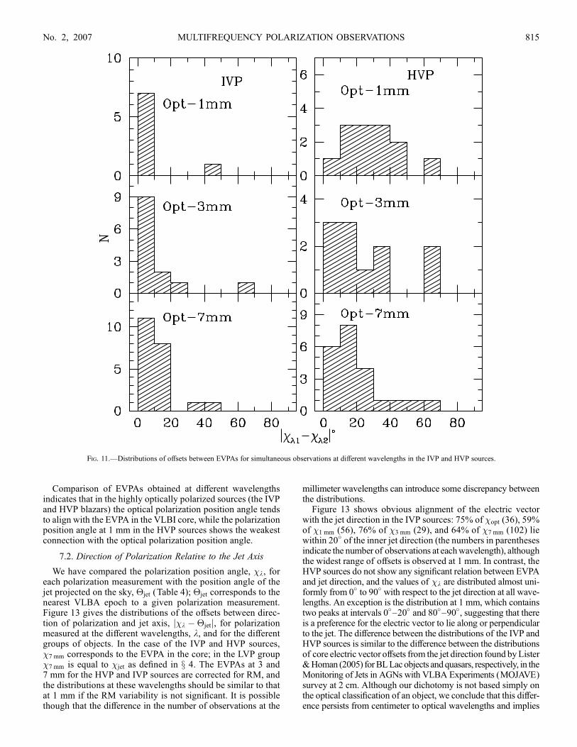
Comparison of EVPAs obtained at different wavelengthsindicates that in the highly optically polarized sources (the IVPand HVP blazars) the optical polarization position angle tendsto align with the EVPA in the VLBI core, while the polarizationposition angle at 1 mm in the HVP sources shows the weakestconnection with the optical polarization position angle.

7.2. Direction of Polarization Relative to the Jet Axis

We have compared the polarization position angle, �k, foreach polarization measurement with the position angle of thejet projected on the sky, �jet (Table 4); �jet corresponds to thenearest VLBA epoch to a given polarization measurement.Figure 13 gives the distributions of the offsets between direc-tion of polarization and jet axis, j�k ��jetj, for polarizationmeasured at the different wavelengths, k, and for the differentgroups of objects. In the case of the IVP and HVP sources,�7 mm corresponds to the EVPA in the core; in the LVP group�7 mm is equal to �jet as defined in x 4. The EVPAs at 3 and7 mm for the HVP and IVP sources are corrected for RM, andthe distributions at these wavelengths should be similar to thatat 1 mm if the RM variability is not significant. It is possiblethough that the difference in the number of observations at the

millimeter wavelengths can introduce some discrepancy betweenthe distributions.

Figure 13 shows obvious alignment of the electric vectorwith the jet direction in the IVP sources: 75% of �opt (36), 59%of �1 mm (56), 76% of �3 mm (29), and 64% of �7 mm (102) liewithin 20� of the inner jet direction (the numbers in parenthesesindicate the number of observations at eachwavelength), althoughthe widest range of offsets is observed at 1 mm. In contrast, theHVP sources do not show any significant relation between EVPAand jet direction, and the values of �k are distributed almost uni-formly from 0� to 90� with respect to the jet direction at all wave-lengths. An exception is the distribution at 1 mm, which containstwo peaks at intervals 0�Y20� and 80�Y90�, suggesting that thereis a preference for the electric vector to lie along or perpendicularto the jet. The difference between the distributions of the IVP andHVP sources is similar to the difference between the distributionsof core electric vector offsets from the jet direction found byLister&Homan (2005) forBLLac objects andquasars, respectively, in theMonitoring of Jets in AGNs with VLBA Experiments (MOJAVE)survey at 2 cm. Although our dichotomy is not based simply onthe optical classification of an object, we conclude that this differ-ence persists from centimeter to optical wavelengths and implies

Fig. 11.—Distributions of offsets between EVPAs for simultaneous observations at different wavelengths in the IVP and HVP sources.


differences in the magnetic fields and/or processes responsiblefor the polarized emission in these objects.

In the LVP sources the distributions of j�k ��jetj at opticaland 1 mm wavelengths do not support a connection of the EVPAwith the jet direction, although the polarization at 1 mm seemsto avoid being parallel to the jet. The polarization position angleat 3 mm and in the inner jet at 7mm clearly reveals a preferentialdirection perpendicular to the jet: 89% of �3 mm (9) and 62% of�7 mm (47) values lie within 70�Y90� of the jet axis. Althoughthe distribution at 3 mm is dominated by the observations of3C 273, all three sources make a significant contribution in thepronounced peak of the distribution at 7 mm.

The properties of polarization position angle with respect tothe jet direction are distinct for each group: good alignment ofthe electric vector with the jet direction at all wavelengths in the

IVP sources, chaotic behavior of the electric vector in the HVPblazars independent of frequency, and electric vector prefer-entially transverse to the jet direction in the LVP objects at 3 mmand in the inner jet at 7 mm. It is noteworthy that the dichotomyat high frequencies is similar to that found for regions fartherout in the jet at lower frequencies (Cawthorne et al. 1993; Lister& Homan 2005).

8. INTERPRETATION

8.1. Magnetic Turbulence

Our data are consistent with the assumption that we observeincoherent synchrotron radiation across the wavelength rangefrom optical to millimeter wavelengths. A uniform magneticfield throughout the emission region yields the maximum pos-sible degree of polarization, mmax ¼ (� þ 1)/(� þ 5/3) (e.g.,Pacholczyk 1970), which is �70% at millimeter wavelengths(� � 0:5; Table 6) and �78% in the optical band (� � 1:4;Impey & Neugebauer 1988). Such a high degree of polarizationhas never been observed in a blazar. The polarization can be sig-nificantly reduced if the emission region is turbulent enough thatit is composed of many cells, each containing a roughly uniformmagnetic field that is randomly oriented relative to that in othercells (Burn 1966; Burch 1979). For N cells within a telescopebeam, the fractional polarization is given by the equation (Hughes& Miller 1991)

m � mmax=ffiffiffiffiN

p� mmax=

ffiffiffiffiffiffiffi2N

p: ð3Þ

The results obtained in xx 6Y7 indicate that the polarizationproperties, and therefore magnetic field structure, of our sourcesare comparable within a group but diverse across different groupsin our classification scheme. We have calculated for each groupthe mean and standard deviation of the maximum degree of po-larization over sources measured at each wavelength, hmmax

k i ��maxk , as well as similar values, hmmin

k i � �mink , for the minimum

degree of polarization. The values, given in Table 12, show thatboth the maximum and minimum degree of polarization increasewith frequency except for the LVP group,withinwhich the opticalpolarization is similar to the polarization in the VLBI core. At agiven frequency, the fractional polarization is lowest for the LVPobjects and highest for the IVP sources, independent of whetherthe polarization is near the minimum or maximum. We use themeans and standard deviations given in Table 12 and equation (3)to determine whether the observed parameters can be derivedwithin a cellular model. Table 12 lists the number of cells,N max

cell

and N mincell , that result in the observed degree of polarization

under this model.We can calculate the number of turbulent cells for any degree

of polarization; however, the same number should account forthe standard deviation as well. We find that this requirement isnot satisfied at high-polarization states, where the standard de-viation is significantly lower than the model predicts. In low-polarization states, the requirement holds at all wavelengthsexcept 1 mm, where the standard deviations for the LVP andHVP sources are slightly lower than expected according to thederived number of cells. This suggests that the high-polarizationstates involve an additional process that provides some order tothe magnetic field, while the low-polarization states can be ex-plained within the cellular model.Three interesting consequences follow from analysis of

Table 12. First, the observed difference in degree of polarizationamong the groups of objects suggests that the emission regionsof the LVP and HVP sources contain more turbulent cells than

Fig. 12.—Distributions of offsets between EVPAs for simultaneous obser-vations at different wavelengths in the LVP sources. The polarization positionangle at 7 mm corresponds to the EVPA in the inner jet.

JORSTAD ET AL.816

Fig. 13.—Distributions of offsets between polarization position angle and jet direction.

TABLE 12

Average Values of Fractional Polarization

Group Quantity Opt 1 mm 3 mm 7 mm

LVP ...................... hmmaxi (%) 1.4 � 1.2 (1.0) 10.2 � 2.1 (7.2) 2.8 � 0.9 (2.0) 1.4 � 0.3 (1.0)

N maxcell 3104 47 625 2500

HVP...................... hmmaxi (%) 11.4 � 7.5 (8.1) 8.6 � 1.8 (6.1) 3.1 � 1.3 (2.2) 6.0 � 1.9 (4.2)

N maxcell 47 66 510 136

IVP ....................... hmmaxi (%) 29.0 � 11.3 (20) 16.8 � 9.4 (11) 9.1 � 2.4 (6.4) 7.5 � 2.1 (5.3)

N maxcell 8 18 59 87

LVP ...................... hmmini (%) 0.4 � 0.3 (0.3) 1.3 � 0.3 (0.9) 0.9 � 0.6 (0.6) 0.1 � 0.1 (0.1)

Nmincell 38025 2900 6050 490000

HVP...................... hmmini (%) 1.7 � 1.2 (1.2) 1.6 � 0.8 (1.1) 0.6 � 0.3 (0.4) 0.5 � 0.2 (0.3)

Nmincell 2105 1914 13611 19600

IVP ....................... hmmini (%) 10.6 � 8.2 (7.5) 4.0 � 3.1 (2.8) 3.2 � 2.1 (2.3) 2.0 � 1.0 (1.4)

Nmincell 54 306 480 1225

Note.—Values in parentheses indicate standard deviations expected from the cellular model with number of cells derived from thefractional polarization; see text.

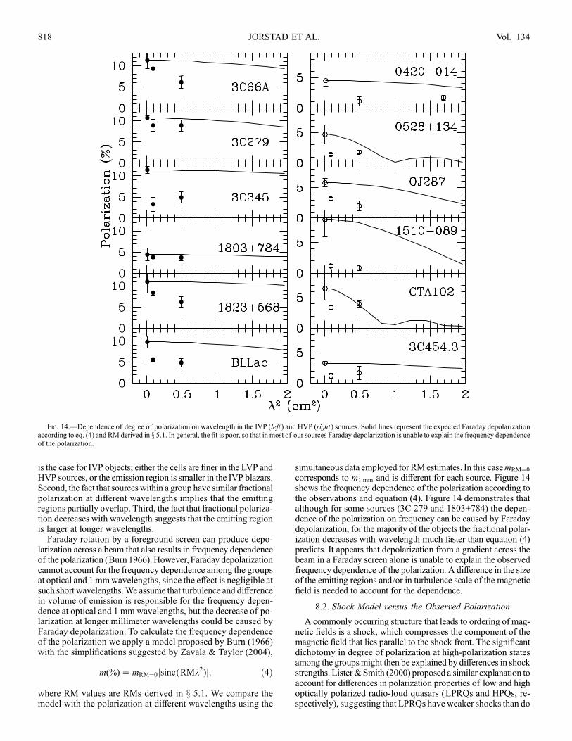
is the case for IVP objects; either the cells are finer in the LVP andHVP sources, or the emission region is smaller in the IVP blazars.Second, the fact that sourceswithin a group have similar fractionalpolarization at different wavelengths implies that the emittingregions partially overlap. Third, the fact that fractional polariza-tion decreases with wavelength suggests that the emitting regionis larger at longer wavelengths.

Faraday rotation by a foreground screen can produce depo-larization across a beam that also results in frequency dependenceof the polarization (Burn 1966).However, Faraday depolarizationcannot account for the frequency dependence among the groupsat optical and 1 mmwavelengths, since the effect is negligible atsuch short wavelengths.We assume that turbulence and differencein volume of emission is responsible for the frequency depen-dence at optical and 1 mm wavelengths, but the decrease of po-larization at longer millimeter wavelengths could be caused byFaraday depolarization. To calculate the frequency dependenceof the polarization we apply a model proposed by Burn (1966)with the simplifications suggested by Zavala & Taylor (2004),

m(%) ¼ mRM¼0jsinc(RMk2)j; ð4Þ

where RM values are RMs derived in x 5.1. We compare themodel with the polarization at different wavelengths using the

simultaneous data employed for RMestimates. In this casemRM¼0

corresponds to m1 mm and is different for each source. Figure 14shows the frequency dependence of the polarization according tothe observations and equation (4). Figure 14 demonstrates thatalthough for some sources (3C 279 and 1803+784) the depen-dence of the polarization on frequency can be caused by Faradaydepolarization, for the majority of the objects the fractional polar-ization decreases with wavelength much faster than equation (4)predicts. It appears that depolarization from a gradient across thebeam in a Faraday screen alone is unable to explain the observedfrequency dependence of the polarization. A difference in the sizeof the emitting regions and/or in turbulence scale of the magneticfield is needed to account for the dependence.

8.2. Shock Model versus the Observed Polarization

A commonly occurring structure that leads to ordering of mag-netic fields is a shock, which compresses the component of themagnetic field that lies parallel to the shock front. The significantdichotomy in degree of polarization at high-polarization statesamong the groupsmight then be explained by differences in shockstrengths. Lister& Smith (2000) proposed a similar explanation toaccount for differences in polarization properties of low and highoptically polarized radio-loud quasars (LPRQs and HPQs, re-spectively), suggesting that LPRQs have weaker shocks than do

Fig. 14.—Dependence of degree of polarization on wavelength in the IVP (left ) and HVP (right ) sources. Solid lines represent the expected Faraday depolarizationaccording to eq. (4) and RM derived in x 5.1. In general, the fit is poor, so that in most of our sources Faraday depolarization is unable to explain the frequency dependenceof the polarization.


HPQs.We use the Hughes &Miller (1991) approach to estimatethe shock strength for the sources in our sample,

m � � þ 1

� þ 5=3

(1� ��2) sin2�0

2� (1� ��2) sin2�0 ; ð5Þ

where � ¼ nshocked /nunshocked and n is the number density of theplasma; �0 is the viewing angle of the jet corrected for relativ-istic aberration: �0 ¼ tan�1fsin�o /�½cos�o � (1� ��2)1

=2 g,where � is the bulk Lorentz factor and �o is the viewing angleof the jet in the observer’s frame. The use of the viewing anglewith respect to the jet axis in the formula applies to a transverseplane-wave shock, and the formula is valid for a shock propa-gating through a plasmawith a completely chaotic magnetic field.The maximum possible polarization should be seen when theshock is viewed along the plane of compression in the frameof the shock (i.e., �0 � 90

�). Columns (3), (5), (7), and (9) of

Table 13 list the values of the estimated shock strength � basedon the maximum observed degree of polarization (cols. [2], [4],[6], and [8]) at each wavelength. Column (10) contains theviewing angle�0 in the shock frame, as derived from the valuesof h�oi and h�i obtained for each object in J05. Because we donot have multicolor data in the optical region, the computationof � adopts�opt=1 mm for the value of�opt, while at 1, 3, and 7 mmwe use the three-point spectral index �mm derived from all threemillimeter wavelengths (see Table 6).

The shock strengths listed in Table 13 are similar among thesources and rather low, � � 1:1Y1:2, and hence cannot be theprimary reason behind the diversity in degree of polarization.Instead, we can explain this by differences in viewing angle rel-ative to the plane of compression, although a very high level ofpolarization (m k 30%) does require much stronger compression,� � 2Y3. Note that for 3C 66A J05 found a significant range ofapparent speeds of superluminal components, from 1.5c to 27c.We use the Lorentz factor and viewing angle that corresponds tothe average of � and �o derived for the fast components only(� ¼ 27:8 and�o ¼ 3:3�), because h�i and h�oi averaged overall components (J05) fails to produce polarization as large asthat observed for any given value of �. The latter is the case for1823+568 as well. However, for 1823+568 moving componentswithin 1 mas of the core were not observed (J05) and the jet

parameters are obtained using kinematics of two componentsat �2 mas from the core. This implies that � and �o in theVLBI core of 1823+568 might be different from those derivedin J05.

Figure 15 shows the dependence between bulk Lorentz factorand polarization variability index. There is a correlation be-tween � and V

popt (r ¼ 0:53, � ¼ 0:1) and between � and V

p7 mm

(r ¼ 0:72, � ¼ 0:05). AlthoughV p3 mm correlateswith� (r ¼ 0:42),

this correlation is significant only at a level � > 0:15. In theplane-wave shock model, the correlation is expected if the mini-mum degree of polarization corresponds to unshocked plasmaand the maximum to faster, shocked plasma. In the shock-in-jetmodel, polarized regions at different wavelengths are partiallycospatial and have essentially the same bulk Lorentz factor.Radiative energy losses of the relativistic electrons cause theshorter wavelength emission to occupy a smaller fraction of thefull shocked region seen at longer wavelengths (Marscher &Gear 1985;Marscher 1996). Since the shorter wavelength emis-sion is assumed to originate from fewer turbulent cells, the degreeof polarization and its variability should increase with decreasingwavelength according to equation (3).

Contrary to what we find at the other wavelengths, the po-larization variability index at 1 mm does not correlate with theLorentz factor (r ¼ �0:12; see Fig. 15). Furthermore, accordingto Table 12, the number of cells needed in the high-polarizationstate at 1 mm is only slightly larger than, or comparable to, thatin the optical region. This conflicts with the expectations of theshock model, although N max

cell at 1 mm is much smaller than at 3and 7 mm, in keeping with the model. The partial discrepancysuggests that another emission component in addition to trans-verse shocks is prominent at 1 mm. A primary candidate is the‘‘true’’ core, i.e., the bright, narrow end of the jet when observedat a wavelength where the emission is completely optically thin(Fig. 16). At wavelengths of 3 mm and longer, what appears tobe the core is most likely a location at or outside the point wherethe optical depth (�) � 1. The fact that the optical polarizationdoes show the correlation, as well as the best alignment ofposition angle with the electric vector in the core at 7 mm, impliesthatmost of the nonthermal optical emission arises in shocks closeto the 7 mm core rather than in the ‘‘true’’ core. This suggests thatthe ‘‘true’’ core does not possess relativistic electrons energeticenough to produce the optical synchrotron emission.

TABLE 13

Derived Shock Strength

Source

(1)

mmaxopt

(%)

(2)

�opt(3)

mmax1 mm

(%)

(4)

�1 mm

(5)

mmax3 mm

(%)

(6)

�3 mm

(7)

mmax7 mm

(%)

(8)

�7 mm

(9)

�0

(deg)

(10)

3C 66A....................... 29.7 1.94 36.4 3.20 9.3 1.21 7.7 1.17 116.0

3C 111........................ 3.1 1.05 12.2 1.22 2.3 1.04 0.5 1.01 108.3

0420�014 .................. 26.2 1.81 7.5 1.18 0.5 1.01 3.3 1.07 59.8

3C 120 ....................... 0.5 1.01 11.1 1.30 2.1 1.05 1.1 1.02 124.5

0528+134 ................... 7.0 1.15 12.1 1.32 1.4 1.03 5.4 1.12 57.0

OJ 287........................ 15.6 1.24 6.9 1.11 4.0 1.06 5.0 1.08 85.3

3C 273 ....................... 0.5 1.01 7.2 1.11 4.0 1.06 1.6 1.02 96.8

3C 279 ....................... 39.2 3.49 10.9 1.30 13.7 1.40 6.9 1.17 59.2

1510�089 .................. 4.1 1.06 9.7 1.15 4.8 1.07 9.7 1.15 83.6

3C 345 ....................... 38.3 1.78 11.4 1.18 8.1 1.13 9.6 1.15 82.7

1803+784 ................... . . . . . . 11.3 1.24 5.9 1.11 5.7 1.11 67.1

1823+568 ................... 29.8 . . . 20.3 . . . 9.9 1.91 10.6 2.08 37.0

BL Lac ....................... 7.8 1.12 10.4 1.18 7.8 1.13 4.9 1.08 86.3

CTA 102 .................... 9.4 1.14 7.1 1.12 3.4 1.06 6.1 1.10 75.9

3C 454.3 .................... 6.2 1.28 8.5 1.51 1.8 1.07 6.6 1.35 39.0


8.3. Magnetic Field Structure in the Jets

In the shock-in-jet model (e.g.,Marscher&Gear 1985; Hugheset al. 1985), we expect a correlation between total flux and po-larization owing to ordering of the magnetic field in the shockedregion if the quiescent jet has a completely chaotic magnetic field.However, if the magnetic field in the unshocked region possessesa component parallel to the jet axis, a transverse shock will en-hance the total flux but partially cancel the polarization as itcompresses the turbulent component. In this case the polarizedflux will at first decrease as the total flux rises. If the shockedemission grows strong enough that its polarized flux becomesgreater than the initial polarized flux of the ambient jet, theEVPAwill flip by 90

�after a minimum in polarized flux, and the

polarized flux will subsequently grow with the total flux untilthe shocked emission weakens. The initial phase of decline inpolarized fluxmay easily be missed in observations spaced suchas ours. If an oblique shock is responsible for an outburst, itseffect on the polarization will depend on the angle of the shockfront relative to the ordered component of the ambient magneticfield, the viewing angle, and the bulk Lorentz factor of the jet. Itis possible, in some cases, for the net polarization to increase,with the EVPA becoming closer to the position angle of the jetaxis on the sky (Hughes 2005).

Figure 10 shows that the maximum of degree of polarizationin the core at 7 mm tends to occur when the total flux rises, whileat 1 mm the opposite relation is more probable. An increaseof the total flux in the VLBI core is usually connected with theemergence of a new superluminal component from the opticallythick part of the core (see J05). If these components representtransverse shock formation in the jet, they should display electricvectors aligned with the jet axis. On the other hand, �1 mm atminimum flux might reflect the magnetic field direction in theunshocked region. Figure 17 (left panel) displays the distributionsof misalignment angles between the polarization and inner jetdirections at times of minimum observed flux at 1 mm. Figure 17(middle panel ) shows the distributions of offsets between �7 mm

and the local jet direction for each superluminal component listedin Table 5 at the point when we can first separate the knot un-ambiguously from the core on the image (i.e., farther downstreamthan 0.1 mas). Figure 17 (right panel) presents the distribution ofdegree of polarization in the superluminal knots at their maximumtotal flux when the separation from the core >0.1 mas. Figure 17indicates that (1) in the ‘‘quiescent jet’’ (prominent at minimum1 mm flux), the magnetic field aligns with the jet for the LVPand HVP sources but is transverse to the jet in the IVP blazars;(2) in the shocked regions (superluminal knots) of the LVPobjects, the magnetic field is longitudinal or oblique to the jet,

Fig. 15.—Lorentz factor vs. polarization variability index at different wavelengths. Triangles: LVP sources; filled circles: IVP sources; open circles: HVP sources.


while for the IVP and HVP sources, its apparent direction isperpendicular to the jet.

The distributions of offsets between the electric vector and jetdirection obtained for the IVP sources at different wavelengths(Fig. 13), the distribution of EVPAs in the superluminal knots,and the high polarization measured in the knots agree with thecase of magnetic fields lying at oblique angles to the jet axis(Lister et al. 1998). (Relativistic aberration tends to align thepolarization vectors closer to the jet axis, creating the illusion thatthemagnetic fields are closer to transverse than is actually the casein the flow frame of the emitting plasma.) This result matches thefinding for BL Lac objects reported by Aller et al. (2003a, 2005),that both the linear polarization structure in VLBA images and themultifrequency polarized flux light curves obtained with single-dish observations are consistent with the oblique shock hypoth-esis. Note that the IVP sources include most of the BL Lac objectsplus those quasars with similar VLBI polarization structure.

In the HVP sources the distribution of offsets between theelectric vector and jet direction at 1mm is double peaked (Fig. 13),nearly parallel or perpendicular to the jet. According to Figure 17,at minimum flux at 1 mm the magnetic field has a parallel orien-tation, which could be associated with the unshocked plasma. Alongitudinal component of the magnetic field in a quiescent jetcan arise from a velocity shear across the jet flow (Laing 1980).Subtraction of the distribution shown in Figure 17 from thatplotted in Figure 13 produces a distribution for the HVP sourcesat 1 mm that is quite similar to the distribution of the IVP sources.Therefore, the magnetic field in the regions responsible for en-hanced emission, including superluminal knots, lies at a trans-verse or oblique angle to the jet axis, in agreement with the

shock model. The superluminal components in the HVP sources(Fig. 17) have only a moderate degree of polarization (<10%),indicating that even in the shocked region, the magnetic field isfairly turbulent. This is consistent with the high amplitude andshort timescale of the polarization variability seen at all wave-lengths. The existence of a longitudinal component of the mag-netic field in quiescent states suggests that either an increase or adecrease in the degree of polarization is possible when a sourcebrightens, depending on the shock strength responsible for theflux enhancement. This diversity of behavior reduces the pos-sibility of observing a correlation between total flux and frac-tional polarization.

The general misalignment between the inner jet and the po-larization vector in the core at 7 mm and at optical and 3 mmwavelengths for the HVP blazars (Fig. 13) fails to reveal anyconnection between the magnetic field and jet structure. In theshock model the distribution of electric vector offsets is ex-pected to show either a good alignment with the jet direction(transverse or oblique shock; Hughes et al. 1985; Lister et al.1998) or a bimodal shape (conical shock; Cawthorne & Cobb1990; Cawthorne 2006). In the conical shock wave model, theon-axis polarization in the shocked region corresponds to theupstream magnetic field structure, while the off-axis electric fieldvectors are oblique to the axis and cover a wide range of anglesthat depend on the shock cone opening angle and the viewingangle. A slight asymmetry of the jet cross-sectional structurewith respect to the axis should lead to relaxation of the depen-dence of themagnetic field on the jet direction. Another factor thatcan contribute to the spread of�with respect to the jet axis is that,despite the high resolution of the 7 mm images, the jet direction atthe positionwhere the emission occursmight be different from thedirection inferred from the images. The latter implies that HVPsources possess higher bending of the jets on milliarcsecondscales than do IVP sources. Conical shocks might explain theappearance of stationary features in the jet (Gomez et al. 1997;Daly &Marscher 1988), which are common in the HVP sources(J05). This model suggests that the core at 7 mm does not alwaysrepresent the emission from the surface where the optical depth is of order unity. Rather, at any given frequency below the turn-over in the spectrum, it would be either the � 1 surface or thefirst standing conical shock system in the < 1 section of the jet,whichever is stronger. If so, the model would explain why theseparation between the core and closest superluminal knot has afrequency dependence in some sources and not in others (seeMarscher 2006 and references therein).

The distributions of position angle offsets between electricvectors and jet direction in the LVP sources (Figs. 13 and 17)indicate the existence of a persistent longitudinal component ofthe magnetic field in the emission regions at 3 mm, 7 mm, in thequiescent jet, and in shocked regions. The modest degree ofpolarization observed in superluminal components of the LVPsources requires a very turbulent magnetic field even in theshocked region. J05 found that LVP sources have the widest jetopening angle in our sample, and the quasar 3C 273 shows sig-nificant variation in the apparent speed of superluminal compo-nents across the jet. The southern jet components are faster thanthe northern ones by a factor of 3. This suggests that a longitudinalcomponent of themagnetic fieldmight arise fromvelocity shear inthe ambient jet, or from complex evolution of the shock emissionowing to the formation of oblique shocks combined with theeffects of radiative transfer. The latter is seen in the numericalsimulations of Hughes (2005).

Using the parameters of jet components B1 and B2 in thequasar 3C 273 derived in J05 and the polarization information

Fig. 16.—Sketch of the main emission regions in the compact jet compatiblewith the results of our investigation. Note the logarithmic scale of distance fromthe black hole (denoted by the dot at the center of the flared accretion disk). Themagnetic field is a tight helix up to the ‘‘true’’ core at 1 mm, beyond which it ischaotic. The system is symmetric with respect to the accretion disk (only one side isshown). The spectrum of the ambient jet rises gradually up to the peak frequency,atwhich the optical depth at the outer edge of the acceleration zone is of order unity,and cuts off at infrared frequencies. The spectrum of a shock moving through thecore is more highly inverted below the peak, and its high-frequency cutoff extendsbeyond the optical region. Although only one is shown, multiple shocks are oftenpresent at any given time.


given in Table 5, we estimate the distance from the core, �z,where a degree of polarization pwill be obtained as the result ofvelocity shear in the jet flow. We assume that the magnetic fieldstarts out in a turbulent state with cell size �x: �z/�R ��N�Rp/(�x�rel), where �N is the bulk Lorentz factor at thenorthern side of the jet,�R is the half-width of the jet, and �rel

is the relative speed between the northern and southern sides.In the plasma frame on the northern side (subscript N ), �rel ¼(�S � �N )/(1� �N�S), where � ¼ (1� ��2)1

=2. We assumethat the Lorentz factor of knot B1 corresponds to the speed atthe northern side (�N ¼ 8:3) and the Lorentz factor of knot B2gives the speed on the southern side (�S ¼ 13:8). According toTable 5, both components possess a similar maximum polariza-tion ( pB1 ¼ 4:0%, pB2 ¼ 6:2%)when the direction of the electricvector is transverse to the jet axis, so we approximate p � 5%.Note that this polarization is achieved in both knots at the samedistance from the core, �0.8 mas. We use the half-opening andviewing angle of the jet derived in J05 ( ¼ 1:4� and�o ¼ 6:1�,respectively). This exercise gives a ratio�R/�x � 40 and size ofa turbulent cell �x � 0:001 pc. For the quasar 3C 273 we haveobtained several groups of closely spaced observations at 3 mmnear some VLBA epochs (see Table 3). The data reveal a veryshort timescale (computed according to the definition of Burbidgeet al. 1974) of the fractional polarization variability at 3 mm,� tvar � 1:8 days. This yields the size of the region responsiblefor the variability, �xvar � 0:001 pc, which is consistent withthe scale of turbulence in the magnetic field.

In summary, the sources in our sample show significant varietyin the distributions of offsets between polarization position angleand jet direction. The observed behavior can be explained withinthe context of shock waves compressing highly turbulent mag-netic fields and velocity shear stretching field lines along a di-rection parallel to the axis if the jet structure and kinematics onmilliarcsecond scales are taken into account.

8.4. Possibility of an ElectromagneticallyDominated Core at 1 mm

The polarized emission at 1 mm possesses properties distin-guished from the other wavelengths. (1) There is no correlationbetween fractional polarization variability index and Lorentzfactor of the jet. (2) The maximum degree of polarization tendsto occur when the total flux is lower than average. (3) The standarddeviation of the mean of the minimum degrees of polarizationover sources in a variability group is lower than expected in thecellular model of magnetic field structure. An inverse relationshipbetween the degree of polarization and total flux is expected inelectromagnetically dominated (ED) jets (Lovelace&Romanova2003) if the plasma responsible for a rise in the total flux has amore chaotic magnetic field than that of the ED section. This canbe the case even if a shock orders an underlying turbulent field inthe same sense as does themostly toroidal field in the EDportion ofthe jet, since the polarization of the ED region should be quite high.The upstream ED model of the jet is a promising scenario

since it explains the high Lorentz factors of the flow needed to

Fig. 17.—Left panels: Distributions of offsets between polarization position angle at 1 mm and inner jet at minimum flux observed at 1 mm in each source.Middlepanels: Distributions of offsets between polarization position angle at 7 mm and local jet direction for superluminal knots listed in Table 5. Right panels: Distributions ofthe degree of polarization in superluminal knots (one entry for each knot; see text).


produce the high apparent speeds seen in some blazars. Accel-eration of the jet to such high values of � is accomplished by con-version of Poynting flux to flow energy through the Lorentz forcethat occurs on scales that are much larger than the gravitationalradius of the central black hole (e.g., Vlahakis 2006). The tentativeanticorrelation between total flux and degree of polarization at1 mm and rather positive correlation between the values at 3 mmand in the core at 7 mm suggest that the acceleration might endbetween the VLBI cores at 1 and 3 mm. In this case the 1 mmemission region should possess a large-scale, mostly toroidal,magnetic field component, which in the plane of the sky shouldlie either transverse or longitudinal to the jet direction (Lyutikovet al. 2005). This is consistent with the distributions of EVPAsat 1 mm with respect to the jet direction in the IVP and HVPsources, in which emission from the VLBI core at 1 mm seemsto dominate the overall source emission at 1 mm (Fig. 13). If thesection of the jet seen at 3 and 7mm is beyond the transition pointwhere the jet becomesmainly hydrodynamical and turbulent, thenthe polarization behavior at these wavelengths will be similar tothat discussed in xx 8.1Y8.3, with shocks partially ordering therandomly oriented component of the magnetic field. The be-havior of the optical polarization is more similar to that at 3 and7 mm, and the best agreement between polarization positionangles for simultaneous observations is observed between theoptical EVPA and polarization position angle in the core at 7 mm.This suggests that the optical emission originates in shocks at ordownstream of the transition point, e.g., at or between the VLBIcores at 3 and 7 mm, and implies that high-energy particle ac-celeration is more efficient in shocks than in the ED region.

9. SUMMARY

We have performed multifrequency, multiepoch, quasi-simultaneous linear polarization observations of a sample of AGNsthat possess highly relativistic jets and high levels of polarizationat 1 mm. We separate the sample into three groups according tothe pattern of variability of the polarization in the VLBI core at7 mm. This classification appears to be connected with physicaldifferences between the objects. However, the sample is smalland future observations of a larger sample are needed to confirmthe findings. The properties of the groups are as follows:

1. The objects with low variability of polarization (LVP)in the VLBI core unite two radio galaxies with superluminalspeeds on parsec scales and a quasar with low observed opticalpolarization. The LVP sources havemeasured optical polarization<2% and radio core polarization <1% and produce stronglypolarized radio jet components that are responsible for the highpolarization observed at 1 mm. The LVP inner jets are mostlikely subjected to very high RMs, RM > 5 ; 105 rad m�2, thatcause depolarization of the core region at millimeter wave-lengths. The optical nonthermal emission is greatly diluted bynonsynchrotron components, probably associated with the bigblue bump. The parsec-scale jets are characterized by moderateLorentz factors, near the low end of the blazar range, and byviewing and opening angles that are larger than those of a typicalblazar. The distributions of EVPAs at 3 mm and in the inner jetat 7 mm with respect to the jet axis reveal a preferred longitu-dinal component of the magnetic field that can be explained byvelocity shear.

2. The sources with intermediate variability of polarization(IVP) in the VLBI core include BL Lac objects and quasars withpreferred direction of the electric vector at all wavelengths closeto the direction of the inner jet. They possess very high opticalpolarization (k30%) and relatively highly polarized (>2%) VLBI

cores at 7 mm. The polarized and total flux density spectra fromoptical wavelengths to 1 mm suggest that synchrotron compo-nents with fairly flat spectra, � � 0:5, dominate the total emis-sion at these wavelengths. The IVP sources possess a moderateRM, RM P 5 ; 103 rad m�2, in the core, which is consistentwith the lack of emission lines in the spectra of BL Lac objectsowing to a relatively low column density of gas. The radio jetsof the IVP sources are highly relativistic, with � � 10. The align-ment of the polarization with the jet at all wavelengths indicatesthe dominance of a transverse or (in the plasma frame) obliquecomponent of the magnetic field.

3. The category of objects with highly variable polarization(HVP) in the VLBI core consists of the OVV quasars and theBL Lac object OJ 287. These display strong variations in bothdegree and polarization position angle. The very high opticalpolarization seen in the IVP sources occurs in the HVP sources,but, in contrast with the IVP blazars, low polarization (<1%) atmillimeter wavelengths and in the VLBI core is common. Onlya single synchrotron component with a steep spectral index,� � 1:0, is required to produce the polarized emission from op-tical to 1mmwavelengths, although a nonsynchrotron componentcould contribute a small fraction of the total optical emission.The HVP sources possess high RMs in the VLBI core at 7 mm,RM � 3 ; 104 rad m�2, implying that the core is surrounded bydense thermal plasma. The radio jets of the HVP sources haveLorentz factors at the high-end tail of the blazar distribution. Thegeneral misalignment between the polarization position angleand jet direction indicates that there is little, if any, connectionbetween the two.

The diversity of polarization properties of the sources in thesample allows us to establish connections between parametersat different wavelengths. (1) There is good agreement betweenthe optical EVPA and that in the VLBI core at 7 mm for the IVPand HVP blazars. (2) The overall polarization of a source at 1and 3 mm strongly correlates with the degree of polarization inthe inner jet of the LVP sources. (3) The EVPA at 1 and 3 mmcorresponds to that in the inner jet for the LVP sources. (4) There isa strong correlation between the level of polarization variability inthe optical region and in the VLBI core at 7 mm. (5) The opticaland 7mm polarization variability indices correlate with the bulkLorentz factor of the radio jets. (6) The degree of polarizationdecreases withwavelength. (7) The distributions of electric vectoroffsets with respect to the inner jet direction at optical and milli-meter wavelengths are similar within each variability group, withdistinct differences among the three groups.

In general, the time variability across the various wavelengthsfollows the expectations of models in which rather weak shockwaves propagate down a jet containing a turbulent magnetic field.After taking into account relativistic aberration, we find that theshock fronts generally lie at oblique angles to the jet axis.

The correlations that we have uncovered tightly link the emis-sion at optical and 3 mm wavelengths to the VLBI core at 7 mm.At 1 mm there is a possible anticorrelation between total fluxdensity and degree of polarization, but not at 7 or 3 mm. Thissuggests the presence of a well-ordered magnetic field in a regionthat is optically thick at k k 1 mm but does not contain electronswith energies sufficiently high to radiate at optical wavelengths.During outbursts, the 1mmpolarization isweakened by the some-what more weakly polarized emission from a shock movingthrough the downstream portion of the jet where the ambientmagnetic field is chaotic. We suggest that the quasisteady 1 mmemission arises near the end of the section where the jet is accel-erated by magnetic forces, a process that requires a tight helical


field geometry. The acceleration of electrons in this region isapparently inadequate to produce optical synchrotron radiation;shocks might be required to do this. Figure 16 presents a sketchof a relativistic jet to illustrate our interpretation.

Our study demonstrates the utility of multi-wave-band po-larization monitoring of blazars when combined with multiepochimaging of their jets with VLBI at millimeter wavelengths. Fur-ther progress is possible through more intense time and frequencycoverage of a large number of objects.

This material is based on work supported by the NationalScience Foundation under grant AST 04-06865. P. S. S. acknowl-edges support from National Aeronautics and Space Adminis-

tration contract 1256424. T. V. C. and A. M. S. acknowledgesupport through research grants from the UK Particle Physicsand Astronomy Research Council. J. L. G. acknowledges sup-port from the Spanish Ministerio de Educacion y Ciencia andthe European Fund for Regional Development through grantAYA2004-08067-C03-03. We thank Gary Schmidt for the main-tenance and use of the Two-Holer Polarimeter. The VLBA is afacility of the National Radio AstronomyObservatory, operatedby Associated Universities, Inc., under cooperative agreementwith the National Science Foundation. The James Clerk MaxwellTelescope is operated by The Joint Astronomy Centre on behalfof the Particle Physics and Astronomy Research Council of theUnited Kingdom, the Netherlands Organisation for ScientificResearch, and the National Research Council Canada.

REFERENCES

Aller, H. D., Aller, M. F., & Hughes, P. A. 2003a, in ASP Conf. Ser. 300,Astronomy at the Fringe, ed. J. A. Zensus, M. H. Cohen, & E. Ross (SanFrancisco: ASP), 143

Aller, H. D., Aller, M. F., Hughes, P. A., Homan, D. C., Wardle, J. F. C., &Roberts, H. D. 2005, in ASP Conf. Ser. 340, Future Directions in HighResolution Astronomy: The 10th Anniversary of the VLBA, ed. J. D.Romney & M. J. Read (San Francisco: ASP), 165

Aller, M. F., Aller, H. D., & Hughes, P. A. 2003b, ApJ, 586, 33Attridge, J. M., Wardle, J. F. C., & Homan, D. C. 2005, ApJ, 633, L85Begelman, M. C., Blandford, R. D., & Rees, M. J. 1984, Rev. Mod. Phys., 56,255

Bowker, A. H., & Lieberman, G. J. 1972, Engineering Statistics (EnglewoodCliffs: Prentice-Hall)

Burbidge, G. R., Jones, T. W., & Odell, S. L. 1974, ApJ, 193, 43Burch, S. F. 1979, MNRAS, 186, 519Burn, B. J. 1966, MNRAS, 133, 67Cawthorne, T. V. 2006, MNRAS, 367, 851Cawthorne, T. V., & Cobb, W. K. 1990, ApJ, 350, 536Cawthorne, T. V., & Wardle, J. F. C. 1988, ApJ, 332, 696Cawthorne, T. V., Wardle, J. F. C., Roberts, D. H., & Gabuzda, D. C. 1993,ApJ, 416, 519

Daly, R. A., & Marscher, A. P. 1988, ApJ, 334, 539D’Arcangelo, F. D., et al. 2007, ApJ, 659, L107Gabuzda, D. C. 2006, in ASP Conf. Ser. 345, From Clark Lake to the LongWavelength Array: Bill Erickson’s Radio Science, ed. N. Kassim et al. (SanFrancisco: ASP), 264

Gabuzda, D. C., Rastorgueva, E. A., Smith, P. S., & O’Sullivan, S. P. 2006,MNRAS, 369, 1596

Gabuzda, D. C., Sitko, M. L., & Smith, P. S. 1996, AJ, 112, 1877Gomez, J. L., Marscher, A. P., Alberdi, A., Jorstad, S. G., & Garcıa-Miro, C.2000, Science, 289, 2317

Gomez, J. L., Martı, J. M., Marscher, A. P., Ibanez, J. M., & Alberdi, A. 1997,ApJ, 482, L33

Gracia, J., Tsinganos, K., & Bogovalov, S. V. 2005, A&A, 442, L7Greaves, J. S., et al. 2003, MNRAS, 340, 353Hagen-Thorn, V. A. 1980, Ap&SS, 73, 279Holland, W. S., et al. 1999, MNRAS, 303, 659Hughes, P. A. 2005, ApJ, 621, 635Hughes, P. A., Aller, H. D., & Aller, M. F. 1985, ApJ, 298, 301———. 1989, ApJ, 341, 68Hughes, P. A., & Miller, L. 1991, in Beams and Jets in Astrophysics, ed. P. A.Hughes (Cambridge: Cambridge Univ. Press), 1

Impey, C. D., Malkan, & M. A., & Tapia, S. 1989, ApJ, 347, 96Impey, C. D., & Neugebauer, G. 1988, AJ, 95, 307Jorstad, S. G., Marscher, A. P., Mattox, J. R., Wehrle, A. E., Bloom, S. D., &Yurchenko, A. V. 2001, ApJS, 134, 181

Jorstad, S. G., et al. 2005, AJ, 130, 1418 (J05)Kellermann, K. I., et al. 2004, ApJ, 609, 539Laing, R. A. 1980, MNRAS, 193, 439Landolt, A. U. 1983, AJ, 88, 439Lister, M. L. 2006, in ASP Conf. Ser. 350, Blazar Variability Workshop II:Entering the GLAST Era, ed. H. R. Miller et al. (San Francisco: ASP), 139

Lister, M. L., & Homan, D. C. 2005, AJ, 130, 1389Lister, M. L., Marscher, A. P., & Gear, W. K. 1998, ApJ, 504, 702Lister, M. L., & Smith, P. S. 2000, ApJ, 541, 66Lobanov, A. P. 1998, A&A, 330, 79Lovelace, R. V. E., & Romanova, M. M. 2003, ApJ, 596, L159Lyutikov, M., Pariev, V. I., & Gabuzda, D. C. 2005, MNRAS, 360, 869Marscher, A. P. 1996, in ASP Conf. Ser. 110, Blazar Continuum Variability, ed.H. R. Miller, J. R. Webb, & J. C. Noble (San Francisco: ASP), 248

———. 2006, in AIP Conf. Proc. 856, Relativistic Jets: The Common Physicsof AGN, Microquasars, and Gamma Ray Bursts, ed. P. A. Hughes & J. N.Bregman (New York: AIP), 1

Marscher, A. P., & Gear, W. K. 1985, ApJ, 298, 114McKinney, J. C. 2006, MNRAS, 367, 1797Mead, A. R. G., Ballard, K. R., Brand, P. W. J. L., Hough, J. H., Brindle, C., &Bailey, J. A. 1990, A&AS, 83, 183

Meier, D. L., Koide, S., & Uchida, Y. 2001, Science, 291, 84Meier, D. L., & Nakamura, N. 2006, in ASP Conf. Ser. 350, Blazar VariabilityWorkshop II: Entering the GLAST Era, ed. H. R. Miller et al. (San Francisco:ASP), 195

Moore, M. L., Schmidt, G. D., & West, S. C. 1987, ApJ, 314, 176Nartallo, R., Gear, W. K., Murray, A. G., Robson, E. I., & Hough, J. H. 1998,MNRAS, 297, 667

Pacholczyk, A. G. 1970, Radio Astrophysics (San Francisco: W. H. Freeman)Savolainen, T., Wiik, K., Valtaoja, E., Jorstad, S. G., & Marscher, A. P. 2002,A&A, 394, 851

Sitko, M. L., Schmidt, G. D., & Stein, W. A. 1985, ApJS, 59, 323Smith, P. S. 1996, in ASP Conf. Ser. 110, Blazar ContinuumVariability, ed. H. R.Miller, J. R. Webb, & J. C. Noble (San Francisco: ASP), 135

Smith, P. S., & Balonek, T. J. 1998, PASP, 110, 1164Smith, P. S., Balonek, T. J., Elston, R., & Heckert, P. A. 1987, ApJS, 64, 459Smith, P. S., Balonek, T. J., Heckert, P. A., Elston, R., & Schmidt, G. D. 1985,AJ, 90, 1184

Smith, P. S., Elston, R., Berriman, G., Allen, R. G., & Balonek, T. J. 1988, ApJ,326, L39

Smith, P. S., Hall, P. B., Allen, R. G., & Sitko, M. L. 1992, ApJ, 400, 115Smith, P. S., Schmidt, G. D., & Allen, R. G. 1993, ApJ, 409, 604Taylor, G. B. 1998, ApJ, 506, 637———. 2000, ApJ, 533, 95Vlahakis, N. 2006, in ASP Conf. Ser. 350, Blazar Variability Workshop II:Entering the GLAST Era, ed. H. R. Miller et al. (San Francisco: ASP), 169

Vlahakis, N., & Konigl, A. 2004, ApJ, 605, 656Wardle, J. F. C., Cawthorne, T. V., Roberts, D. H., & Brown, L. F. 1994, ApJ,437, 122

Wardle, J. F. C., & Kronberg, P. P. 1974, ApJ, 194, 249Wills, B. J., Wills, D., Breger, M., Antonucci, R. R. J., & Barvainis, R. 1992,ApJ, 398, 454

———. 2003, ApJ, 589, 126Zavala, R. T., & Taylor, G. B. 2003, ApJ, 589, 126———. 2004, ApJ, 612, 749———. 2005, ApJ, 626, L73

JORSTAD ET AL.824

Multiwaveband polarimetric observations of 15 active ...

Documents

Transcript of Multiwaveband polarimetric observations of 15 active ...