Multimedia DataDCT Image Compression

Dr Sandra I. Woolley

http://www.eee.bham.ac.uk/woolleysi

S.I.Woolley@bham.ac.uk

Electronic, Electrical and Computer Engineering

Contents The philosophy behind the lossy

of processes of DCT image compression.

A summary of the processes involved in DCT image compression.

Consideration of DCT ringing and blocking compression artefacts; their appearance and their origin.

Lossy DCT Image Compression The lossy DCT method

compression method is widely used in current standards. For example, JPEG images and MPEG-1 and MPEG-2 (DVD) videos.

The image here is increasingly compressed from left to right.

Blocking artefacts are visible. Ringing artefacts can also be seen around edges.

This lecture will explain how the method works and how these artefacts are caused.

Rate/Distortion As we have seen, quality can fall

rapidly as shown by the steep slope of rate/ distortion graph.

The DCT methods typically* work well up to around 10:1 compression ratios and then quality falls rapidly beyond this.

*Note – the original quality and image type are important considerations.

a) Original b) CR 8:1

c) CR 11.6:1 d) CR 13.6:1

e) CR 14.2:1 f) Difference a-e

g) CR=8:1 with Channel Error

DCT Compression

CR=8:1

DCT Compression

CR=12:1

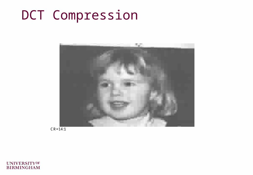
DCT Compression

CR=14:1

DCT Compression

DCT Image Compression The philosophy behind

DCT image compression is that the human eye is less sensitive to higher-frequency information and also more sensitive to intensity than to colour.

The examples shown here are from from Dr Flowers’ MPEG slides showing the effects of percentage reduction of colour.

Original (100%) 0.5 UV (25%) 0.25 UV (6.25%)

0.2 UV (4%) 0.1 UV (1%) 0.0 UV (0%)

DCT Image Compression The DCT method is an example of a transform

method. Rather than simply trying to compress the pixel values directly, the image is first TRANSFORMED into the frequency domain. Compression can now be achieved by more coarsely quantizing the large amount of high-frequency components usually present.

Firstly, the image must be transformed into the frequency domain. This is done in blocks across the whole image.

The JPEG* standard algorithm for full-colour and grey-scale image compression is a DCT compression standard that uses 8x8 blocks.

It was not designed for graphics or line drawings and is not suited to these image types.

*Joint [CCITT and ISO] Photographic Experts Group

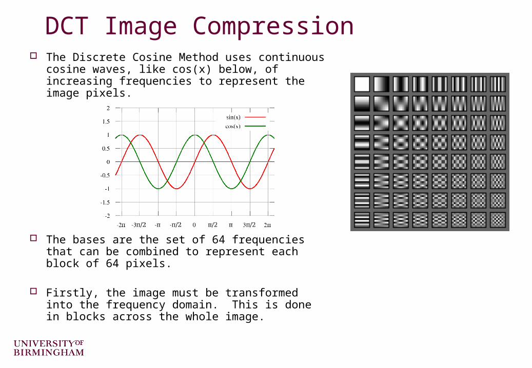
DCT Image Compression The Discrete Cosine Method uses continuous

cosine waves, like cos(x) below, of increasing frequencies to represent the image pixels.

The bases are the set of 64 frequencies that can be combined to represent each block of 64 pixels.

Firstly, the image must be transformed into the frequency domain. This is done in blocks across the whole image.

The Discrete Cosine Transform Bases

Low frequency

High frequency

The DCT Take each 8x8 pixel block and

represent it as amounts (coefficients) of the basis functions (the frequency set).

– represent the 8x8 pixels as amounts of lowest frequency (the average or DC value) through to the highest frequency

– 64 pixels values are TRANSFORMED into 64 coefficients which represent the amount of each frequency.

DCT Image Compression The DCT itself does not achieve compression, but

rather prepares the image for compression.

Once in the frequency domain the image's high-frequency coefficients can be coarsely quantised so that many of them (>50%) can be truncated to zero.

The coefficients can then be arranged so that the zeroes are clustered (zig-zag collection) and Run-Length Encoded.

The remaining data is then compressed with Huffman coding*.

*The JPEG standard actually specifies many variants which have not been widely used. For example, a more efficient algorithm than Huffman, called arithmetic coding, is a standard variant, but there are several patents on this method. We usually refer to the JPEG baseline algorithm if there is a possibility of confusion between variants.

The Baseline JPEG Standard Quantization Matrix - determined by subjective testing -(for interest only)

16 11 10 16 24 40 51 61

12 12 14 19 26 58 60 55

14 13 16 24 40 57 69 56

14 17 22 29 51 87 80 62

18 22 37 56 68 109 103 77

24 35 55 64 81 104 113 92

49 64 78 87 103 121 120 101

72 92 95 98 112 100 103 99

DCT Compression Stages Blocking (8x8) DCT (Discrete Cosine Transformation) Quantization Zigzag Scan DPCM* on the dc value (the average value in the top left) RLE on the ac values (all 63 values which aren’t the dc/

average) Huffman Coding

* DPCM – Differential Pulse Code Modulation – Instead of sending the value send the difference from the previous value.

DCT Mathematics The formula is shown here for interest only (not assessed material).

The Discrete Cosine Transform below takes the pixels(x,y) and generates DCT(i,j) values.

The pixel values can be calculated as shown in the 2nd line, where DCT(i,j) values are used to calculate pixel(x,y) values.

01,02

1)(

2

)12(

2

)12(cos),()()(

2

1),(

2

)12(

2

)12(cos),()()(

2

1),(

1

0

1

0

1

0

1

0

xifelseisxifxC

N

y

N

xjiDCTjCiC

Nyxpixel

N

y

N

xyxpixeljCiC

NjiDCT

N

i

N

j

N

x

N

y

Gibb’s Phenomenon The presence of artefacts around

sharp edges is referred to as Gibb's phenomenon.

These are caused by the inability of a finite combination of continuous functions (like cosines) to describe jump discontinuities (e.g. edges).

At higher compression ratios these losses become more apparent, as do the boundaries of the 8x8 blocks.

The loss of edge clarity can be clearly seen in a difference mapping comparing an original image with its heavily compressed equivalent.

http://www.numerit.com/samples/fours/doc.htm

Original Test ImageAn extreme example for demonstrating Gibb’s phenomenon

Heavily Compressed DCT Image

The Difference (Gibb’s Phenomenon)

Why?

Why do highly corrupted DCT compressed images still retain a vague shadow of the original outline?

Why?

Why do highly corrupted DCT compressed images still retain a vague shadow of the original outline?

Answer: Loss of synchronization within the blocks themselves.

This was answered perfectly by Farzad Hayati who actually retrieved the lost half of the picture shown here on the right. The loss of synchronization is due to lost/corrupted blocks which could be padded. The image would then appear correct with only a missing set of blocks halfway.

Summary The philosophy behind the lossy

processes of DCT image compression.

A summary of the processes involved in DCT image compression.

Consideration of DCT ringing and blocking compression artefacts; their appearance and their origin. For interest …

more links on compression …

http://www.eee.bham.ac.uk/woolleysi/links/datacomp.htm

This concludes our introduction to DCT image compression.

You can find course information, including slides and supporting resources, on-line on the course web page at

Thank You

http://www.eee.bham.ac.uk/woolleysi/teaching/multimedia.htm