Multi Level Tools
36
Introduction A research example from ASR mltcooksd mlt2stage Outlook Multi Level Tools Influential cases in multi level modeling Katja M¨ ohring & Alexander Schmidt GK SOCLIFE, Universit¨ at zu K¨ oln Presentation at the German Stata User Meeting in Berlin, 1 June 2012 1 / 36
Transcript of Multi Level Tools
Introduction A research example from ASR mltcooksd mlt2stage Outlook
Multi Level ToolsInfluential cases in multi level modeling
Katja Mohring & Alexander Schmidt
GK SOCLIFE, Universitat zu Koln
Presentation at the German Stata User Meetingin Berlin, 1 June 2012
1 / 36
Introduction A research example from ASR mltcooksd mlt2stage Outlook
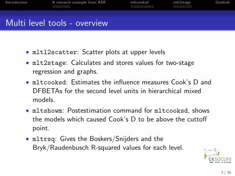
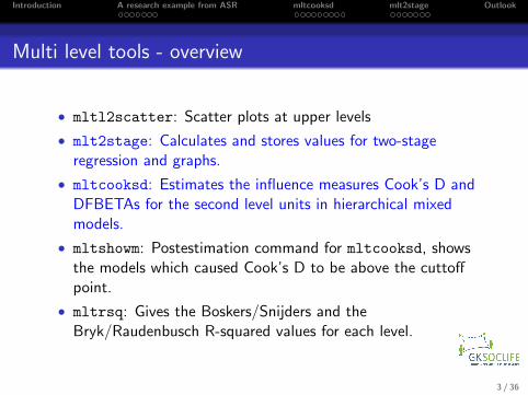
Multi level tools - overview
• mltl2scatter: Scatter plots at upper levels
• mlt2stage: Calculates and stores values for two-stageregression and graphs.
• mltcooksd: Estimates the influence measures Cook’s D andDFBETAs for the second level units in hierarchical mixedmodels.
• mltshowm: Postestimation command for mltcooksd, showsthe models which caused Cook’s D to be above the cuttoffpoint.
• mltrsq: Gives the Boskers/Snijders and theBryk/Raudenbusch R-squared values for each level.
2 / 36
Introduction A research example from ASR mltcooksd mlt2stage Outlook
Multi level tools - overview
• mltl2scatter: Scatter plots at upper levels
• mlt2stage: Calculates and stores values for two-stageregression and graphs.
• mltcooksd: Estimates the influence measures Cook’s D andDFBETAs for the second level units in hierarchical mixedmodels.
• mltshowm: Postestimation command for mltcooksd, showsthe models which caused Cook’s D to be above the cuttoffpoint.
• mltrsq: Gives the Boskers/Snijders and theBryk/Raudenbusch R-squared values for each level.
3 / 36
Introduction A research example from ASR mltcooksd mlt2stage Outlook
Index
1 Introduction
2 A research example from ASR
3 mltcooksd
4 mlt2stage
5 Outlook
4 / 36
Introduction A research example from ASR mltcooksd mlt2stage Outlook
1 Introduction
2 A research example from ASR
3 mltcooksd
4 mlt2stage
5 Outlook
5 / 36
Introduction A research example from ASR mltcooksd mlt2stage Outlook
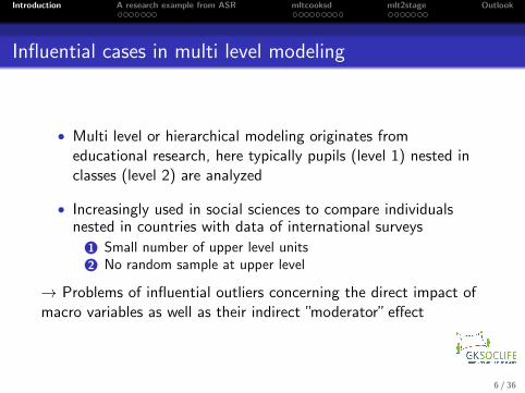
Influential cases in multi level modeling
• Multi level or hierarchical modeling originates fromeducational research, here typically pupils (level 1) nested inclasses (level 2) are analyzed
• Increasingly used in social sciences to compare individualsnested in countries with data of international surveys
1 Small number of upper level units2 No random sample at upper level
→ Problems of influential outliers concerning the direct impact ofmacro variables as well as their indirect ”moderator” effect
6 / 36
Introduction A research example from ASR mltcooksd mlt2stage Outlook
1 Introduction
2 A research example from ASRA research example from the American Sociological ReviewCook’s D and DFBETAS
3 mltcooksdmltcooksd descriptionStata
4 mlt2stagemlt2stage descriptionStata
5 Outlook
7 / 36

Introduction A research example from ASR mltcooksd mlt2stage Outlook
A research example from the American Sociological Review
Why should we consider outliers? A research example
Ruiter and De Graaf (2006): National Context, Religiosity, andVolunteering: Results from 53 Countries. American SociologicalReview.
• Analysis of World Values Survey data with 53 countries
• Dependent variable volunteering
• Independent variable national religious context
• Conclusion: Average church attendance is significantly andpositively related to volunteering
8 / 36
Introduction A research example from ASR mltcooksd mlt2stage Outlook
A research example from the American Sociological Review
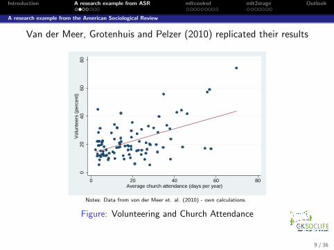
Van der Meer, Grotenhuis and Pelzer (2010) replicated their results
020
4060
80V
olun
teer
s (p
erce
nt)
0 20 40 60 80Average church attendance (days per year)
Notes: Data from von der Meer et. al. (2010) - own calculations.
Figure: Volunteering and Church Attendance
9 / 36
Introduction A research example from ASR mltcooksd mlt2stage Outlook
A research example from the American Sociological Review
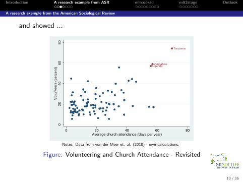
and showed ...
ZimbabweUganda
Tanzania
020
4060
80V
olun
teer
s (p
erce
nt)
0 20 40 60 80Average church attendance (days per year)
Notes: Data from von der Meer et. al. (2010) - own calculations.
Figure: Volunteering and Church Attendance - Revisited
10 / 36
Introduction A research example from ASR mltcooksd mlt2stage Outlook
A research example from the American Sociological Review
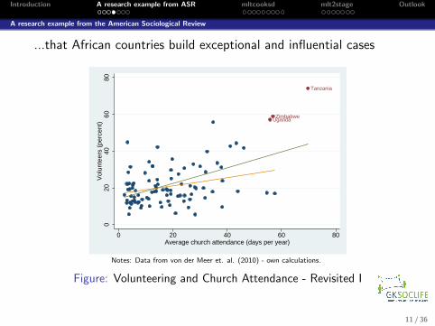
...that African countries build exceptional and influential cases
ZimbabweUganda
Tanzania
020
4060
80V
olun
teer
s (p
erce
nt)
0 20 40 60 80Average church attendance (days per year)
Notes: Data from von der Meer et. al. (2010) - own calculations.
Figure: Volunteering and Church Attendance - Revisited I
11 / 36
Introduction A research example from ASR mltcooksd mlt2stage Outlook
Cook’s D and DFBETAS
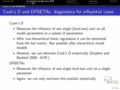
Cook’s D and DFBETAs: diagnostics for influential cases
Cook’s D
• Measures the influence of one single (level-two) unit on allmodel parameters or a subset of parameters
• After non-hierarchical linear regressions it can be estimatedfrom the hat matrix. Not possible after hierarchical mixedmodels
• However, we can estimate Cook’s D empirically (Snijders andBerkhof 2008: 157ff.)
DFBETAs
• Measures the influence of one single level-two unit on a singleparameter
• Again, we can only estimate this statistic empirically
12 / 36
Introduction A research example from ASR mltcooksd mlt2stage Outlook
Cook’s D and DFBETAS
DFBETAs
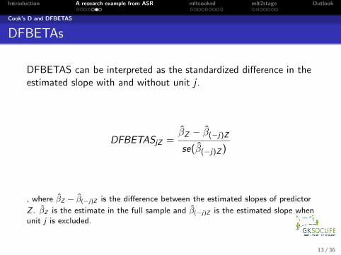
DFBETAS can be interpreted as the standardized difference in theestimated slope with and without unit j .
DFBETASjZ =βZ − β(−j)Z
se(β(−j)Z )
, where βZ − β(−j)Z is the difference between the estimated slopes of predictor
Z . βZ is the estimate in the full sample and β(−j)Z is the estimated slope whenunit j is excluded.
13 / 36

Introduction A research example from ASR mltcooksd mlt2stage Outlook
Cook’s D and DFBETAS
Cook’s D
Fixed part of the model:
CFj =
1
r(β − β
(−j))′S−1F (−j)(β − β
(−j))
, with r =number of fixed parameters. SF (−j) is the variance-covariance matrixafter unit j has been excluded.
Random part of the model:
CRj =
1
p(η − η
(−j))′S−1R(−j)(η − η
(−j))
, with p =number of random parameters.
Overall:
C j =1
r + p(rCF
j + pCRj )
14 / 36
Introduction A research example from ASR mltcooksd mlt2stage Outlook
1 Introduction
2 A research example from ASRA research example from the American Sociological ReviewCook’s D and DFBETAS
3 mltcooksdmltcooksd descriptionStata
4 mlt2stagemlt2stage descriptionStata
5 Outlook
15 / 36
Introduction A research example from ASR mltcooksd mlt2stage Outlook
mltcooksd description
the mltcooksd ado
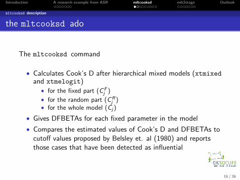
The mltcooksd command
• Calculates Cook’s D after hierarchical mixed models (xtmixedand xtmelogit)
• for the fixed part (CFj )
• for the random part (CRj )
• for the whole model (Cj)
• Gives DFBETAs for each fixed parameter in the model
• Compares the estimated values of Cook’s D and DFBETAs tocutoff values proposed by Belsley et. al (1980) and reportsthose cases that have been detected as influential
16 / 36
Introduction A research example from ASR mltcooksd mlt2stage Outlook
mltcooksd description
mltcooksd syntax
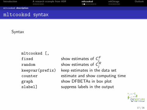
Syntax
mltcooksd [,
fixed show estimates of CFj
random show estimates of CRj
keepvar(prefix) keep estimates in the data setcounter estimate and show computing timegraph show DFBETAs in box plotslabel] suppress labels in the output
17 / 36
Introduction A research example from ASR mltcooksd mlt2stage Outlook
Stata
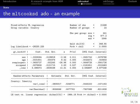
the mltcooksd ado - an example
Mixed-effects ML regression Number of obs = 21498
Group variable: Country Number of groups = 22
Obs per group: min = 441
avg = 977.2
max = 2345
Wald chi2(4) = 948.65
Log likelihood = -28233.225 Prob > chi2 = 0.0000
------------------------------------------------------------------------------
gr_incdiff | Coef. Std. Err. z P>|z| [95% Conf. Interval]
-------------+----------------------------------------------------------------
sex | -.0329264 .0128818 -2.56 0.011 -.0581742 -.0076786
age | .0031901 .000379 8.42 0.000 .0024472 .003933
respincperc | -.0605727 .002245 -26.98 0.000 -.0649728 -.0561726
socspend | .0076906 .0121715 0.63 0.527 -.0161651 .0315463
_cons | 3.086072 .2506038 12.31 0.000 2.594897 3.577246
------------------------------------------------------------------------------
------------------------------------------------------------------------------
Random-effects Parameters | Estimate Std. Err. [95% Conf. Interval]
-----------------------------+------------------------------------------------
Country: Identity |
var(_cons) | .0809317 .0246771 .0445222 .1471162
-----------------------------+------------------------------------------------
var(Residual) | .8058066 .0077762 .7907088 .8211928
------------------------------------------------------------------------------
LR test vs. linear regression: chibar2(01) = 1984.18 Prob >= chibar2 = 0.0000
18 / 36
Introduction A research example from ASR mltcooksd mlt2stage Outlook
Stata
the mltcooksd ado - an example
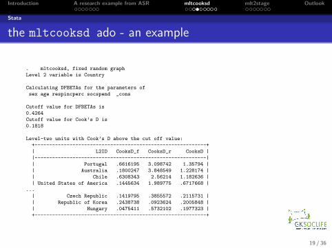
. mltcooksd, fixed random graph
Level 2 variable is Country
Calculating DFBETAs for the parameters of
sex age respincperc socspend _cons
Cutoff value for DFBETAs is
0.4264
Cutoff value for Cook’s D is
0.1818
Level-two units with Cook’s D above the cut off value:
+-----------------------------------------------------------+
| L2ID CooksD_f CooksD_r CooksD |
|-----------------------------------------------------------|
| Portugal .6616195 3.098742 1.35794 |
| Australia .1800247 3.848549 1.228174 |
| Chile .6308343 2.56214 1.182636 |
| United States of America .1445634 1.989775 .6717668 |
...
| Czech Republic .1419795 .3855572 .2115731 |
| Republic of Korea .2438738 .0923624 .2005848 |
| Hungary .0475411 .5732102 .1977323 |
+-----------------------------------------------------------+
19 / 36
Introduction A research example from ASR mltcooksd mlt2stage Outlook
Stata
the mltcooksd ado - an example
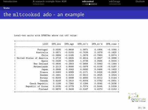
Level-two units with DFBETAs above cut off value:
+-------------------------------------------------------------------------------+
| L2ID DFB_sex DFB_age DFB_re~c DFB_so~d DFB_cons |
|-------------------------------------------------------------------------------|
| Portugal 0.0335 -0.9608 1.3871 0.1956 -0.1090 |
| Australia 0.0871 -0.5155 -0.7639 0.1678 -0.1420 |
| Chile -0.0699 -0.5185 1.3678 -0.7983 0.8374 |
| United States of America 0.2718 -0.5825 -0.4614 0.2827 -0.2996 |
| Spain -0.0439 -1.0599 1.3739 0.0566 0.0000 |
| New Zealand -0.0606 -0.2903 -0.9856 0.0943 -0.1344 |
| Netherlands 0.2113 0.8566 -1.0978 -0.0106 -0.0187 |
| Japan 0.2648 0.3343 0.5692 0.0468 -0.1422 |
| France 0.0492 0.9389 -0.2171 0.0426 -0.0908 |
| Sweden -0.1991 0.5152 -0.9410 -0.2625 0.2324 |
| Norway -0.8209 0.5698 -0.4893 -0.0012 0.0144 |
| Canada 0.4149 0.1610 -0.8004 0.0782 -0.0931 |
| Czech Republic 0.1199 0.7360 0.1394 0.0545 -0.2036 |
| Republic of Korea 0.0035 -0.5778 0.7074 -0.5044 0.5339 |
| Finland -0.5870 0.3408 -0.3167 0.0270 -0.0152 |
+-------------------------------------------------------------------------------+
20 / 36
Introduction A research example from ASR mltcooksd mlt2stage Outlook
Stata
the mltcooksd ado - an example
Repub
lic o
f Kor
ea
Chile
Chile
Repub
lic o
f Kor
ea
Sweden
Norway
cutoff cutoff
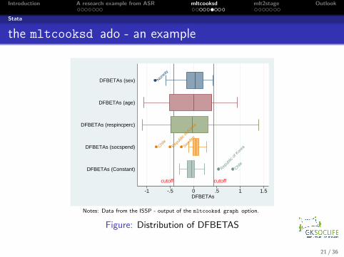
-1 -.5 0 .5 1 1.5DFBETAs
DFBETAs (Constant)
DFBETAs (socspend)
DFBETAs (respincperc)
DFBETAs (age)
DFBETAs (sex)
Notes: Data from the ISSP - output of the mltcooksd graph option.
Figure: Distribution of DFBETAS
21 / 36
Introduction A research example from ASR mltcooksd mlt2stage Outlook
Stata
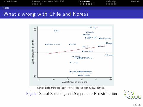
What’s wrong with Chile and Korea?
Australia
Canada
Chile
Czech Republic
Finland
France
Hungary
Ireland
Japan
Republic of Korea
Netherlands
New Zealand
Norway
Poland
Portugal
Slovenia
Spain
Sweden
Switzerland
United States of America
East Germany
Great Britain
2.5
33.
5Le
vel-2
mea
n of
gr_
incd
iff
5 10 15 20 25 30Level-2 mean of socspend
Notes: Data from the ISSP - plot produced with mltl2scatter.
Figure: Social Spending and Support for Redistribution
22 / 36
Introduction A research example from ASR mltcooksd mlt2stage Outlook
Stata
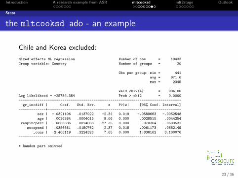
the mltcooksd ado - an example
Chile and Korea excluded:
Mixed-effects ML regression Number of obs = 19433
Group variable: Country Number of groups = 20
Obs per group: min = 441
avg = 971.6
max = 2345
Wald chi2(4) = 984.00
Log likelihood = -25784.384 Prob > chi2 = 0.0000
------------------------------------------------------------------------------
gr_incdiff | Coef. Std. Err. z P>|z| [95% Conf. Interval]
-------------+----------------------------------------------------------------
sex | -.0321106 .0137022 -2.34 0.019 -.0589663 -.0052548
age | .0036384 .0004015 9.06 0.000 .0028515 .0044254
respincperc | -.0656586 .0024008 -27.35 0.000 -.070364 -.0609531
socspend | .0356661 .0150762 2.37 0.018 .0061173 .0652149
_cons | 2.468119 .3224328 7.65 0.000 1.836162 3.100076
------------------------------------------------------------------------------
* Random part omitted
23 / 36
Introduction A research example from ASR mltcooksd mlt2stage Outlook
Stata
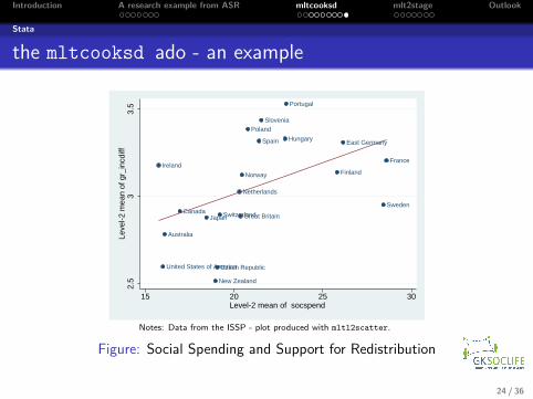
the mltcooksd ado - an example
Australia
Canada
Czech Republic
Finland
France
Hungary
Ireland
Japan
Netherlands
New Zealand
Norway
Poland
Portugal
Slovenia
Spain
Sweden
Switzerland
United States of America
East Germany
Great Britain
2.5
33.
5Le
vel-2
mea
n of
gr_
incd
iff
15 20 25 30Level-2 mean of socspend
Notes: Data from the ISSP - plot produced with mltl2scatter.
Figure: Social Spending and Support for Redistribution
24 / 36

Introduction A research example from ASR mltcooksd mlt2stage Outlook
1 Introduction
2 A research example from ASRA research example from the American Sociological ReviewCook’s D and DFBETAS
3 mltcooksdmltcooksd descriptionStata
4 mlt2stagemlt2stage descriptionStata
5 Outlook
25 / 36
Introduction A research example from ASR mltcooksd mlt2stage Outlook
mlt2stage description
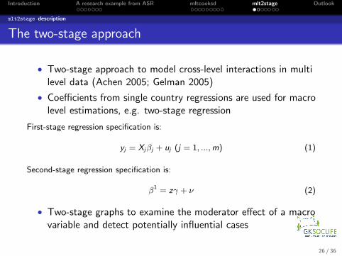
The two-stage approach
• Two-stage approach to model cross-level interactions in multilevel data (Achen 2005; Gelman 2005)
• Coefficients from single country regressions are used for macrolevel estimations, e.g. two-stage regression
First-stage regression specification is:
yj = Xjβj + uj (j = 1, ...,m) (1)
Second-stage regression specification is:
β1 = zγ + ν (2)
• Two-stage graphs to examine the moderator effect of a macrovariable and detect potentially influential cases
26 / 36
Introduction A research example from ASR mltcooksd mlt2stage Outlook
mlt2stage description
the mlt2stage ado
The mlt2stage command
• Calculates and stores the coefficients of country separatelinear and logistic regressions
• Plots the estimated values against a macro level indicator
27 / 36
Introduction A research example from ASR mltcooksd mlt2stage Outlook
Stata
mlt2stage syntax
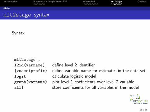
Syntax
mlt2stage ,
l2id(varname) define level 2 identifier[vname(prefix) define variable name for estimates in the data setlogit calculate logistic modelgraph(varname) plot level 1 coefficients over level 2 variableall] store coefficients for all variables in the model
28 / 36
Introduction A research example from ASR mltcooksd mlt2stage Outlook
Stata
the mlt2stage ado - an example
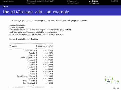
. mlt2stage gr_incdiff respincperc age sex, l2id(Country) graph(socspend)
command:regress
graph:socspend
Two stage calculated for the dependent variable gr_incdiff
and the main explanatory variable respincperc
with the independent variables respincperc age sex
Level 2 variable is Country
-----------------------------------------
Country | mean(coef_g~c)
-------------------------+---------------
Australia | -.0787574
Canada | -.1056875
Chile | -.0109568
Czech Republic | -.0546495
Denmark | -.0809449
Finland | -.0801003
France | -.0712633
Hungary | -.0470008
Ireland | -.0365443
Israel | -.0550879
Japan | -.0374054
Republic of Korea | -.024505
Latvia | -.0239054
Netherlands | -.1280941
New Zealand | -.105004
(...)
----------------------------------------- 29 / 36
Introduction A research example from ASR mltcooksd mlt2stage Outlook
Stata
the mlt2stage ado - an example
-.15
-.1
-.05
0C
oef.
of g
r_in
cdiff
on
resp
incp
erc
5 10 15 20 25 30Social Expenditure as % of GDP
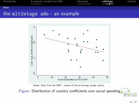
Notes: Data from the ISSP - output of the mlt2stage graph option.
Figure: Distribution of country coefficients over social spending
30 / 36
Introduction A research example from ASR mltcooksd mlt2stage Outlook
Stata
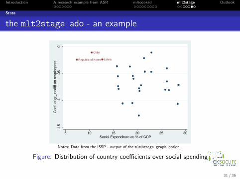
the mlt2stage ado - an example
Chile
Republic of Korea Latvia-.
15-.
1-.
050
Coe
f. of
gr_
incd
iff o
n re
spin
cper
c
5 10 15 20 25 30Social Expenditure as % of GDP
Notes: Data from the ISSP - output of the mlt2stage graph option.
Figure: Distribution of country coefficients over social spending
31 / 36
Introduction A research example from ASR mltcooksd mlt2stage Outlook
Stata
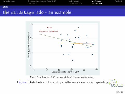
the mlt2stage ado - an example
Chile
Republic of Korea Latvia-.
15-.
1-.
050
Coe
f. of
gr_
incd
iff o
n re
spin
cper
c
5 10 15 20 25 30Social Expenditure as % of GDP
Notes: Data from the ISSP - output of the mlt2stage graph option.
Figure: Distribution of country coefficients over social spending
32 / 36
Introduction A research example from ASR mltcooksd mlt2stage Outlook
1 Introduction
2 A research example from ASR
3 mltcooksd
4 mlt2stage
5 Outlook
33 / 36

Introduction A research example from ASR mltcooksd mlt2stage Outlook
more multi level tools...
mltl2scatter, mlt2stage, mltcooksd, mltshowm,
mltcooksd, mltrsq ...
• Extension of ados for three or more levels• Ado to compare multi level and country FE results• Ado to calculate model fit values for logistic multi level models
34 / 36
Introduction A research example from ASR mltcooksd mlt2stage Outlook
Comments & questions welcome!
→ [email protected], www.katjamoehring.de
→ [email protected], www.alexanderwschmidt.de
35 / 36
Introduction A research example from ASR mltcooksd mlt2stage Outlook
References
Achen, Christopher H. (2005): Two-Step Hierarchical Estimation: Beyond RegressionAnalysis, in: Political Analysis 13(4): 447-456, doi:10.1093/pan/mpi033.
Belsley, David A., Edwin Kuh, and Roy E. Welsch. (1980): Regression Diagnostics:Identifying Influential Data and Sources of Collinearity. New York: John Wiley.
Gelman, Andrew (2005): Two-Stage Regression and Multilevel Modeling: ACommentary, in: Political Analysis 13(4): 459-461, doi: 10.1093/pan/mpi032.
Ruiter, Stijn and Nan Dirk De Graaf (2006): National Context, Religiosity, andVolunteering: Results from 53 Countries. American Sociological Review 71, pp.191210.
Snijders, Tom A. B. and Johannes Berkhof (2008): Diagnostic Checks for MultilevelModels. pp. 457514 in Handbook of Multilevel Analysis, edited by J. De Leeuw and E.Meijer. New York: Springer.
Van der Meer, Tom, Manfred Te Grotenhuis and Ben Pelzer (2010): Influential Casesin Multilevel Modeling: A Methodological Comment. American Sociological Review75: pp. 173-178.
36 / 36