Multi-Dimensional Uniform Initialization Gaussian Mixture ...
20
Sensors 2021, 21, 1283. https://doi.org/10.3390/s21041283 www.mdpi.com/journal/sensors Article Multi-Dimensional Uniform Initialization Gaussian Mixture Model for Spar Crack Quantification under Uncertainty Qiuhui Xu, Shenfang Yuan *, Tianxiang Huang Research Center of Structural Health Monitoring and Prognosis, State Key Lab of Mechanics and Control of Mechanical Structures, Nanjing University of Aeronautics and Astronautics, Nanjing 210016, China; [email protected] (Q.X.); [email protected] (T.H.) * Correspondence: [email protected] Abstract: Guided Wave (GW)-based crack monitoring method as a promising method has been widely studied, as this method is sensitive to small cracks and can cover a wide monitoring range. Online crack quantification is difficult as the initiation and growth of crack are affected by various uncertainties. In addition, crack-sensitive GW features are influenced by time-varying conditions which further increase the difficulty in crack quantification. Considering these uncertainties, the Gaussian mixture model (GMM) is studied to model the probability distribution of GW features. To further improve the accuracy and stability of crack quantification under uncertainties, this paper proposes a multi-dimensional uniform initialization GMM. First, the multi-channel GW features are integrated to increase the accuracy of crack quantification, as GW features from different channels have different sensitivity to cracks. Then, the uniform initialization method is adopted to provide more stable initial parameters in the expectation-maximization algorithm. In addition, the relation- ship between the probability migration index of GMMs and crack length is calibrated with fatigue tests on prior specimens. Finally, the proposed method is applied for online crack quantification on the notched specimen of an aircraft spar with complex fan-shaped cracks under uncertainty. Keywords: structural health monitoring; guided wave; Gaussian mixture model; crack quantification; uncertainty; time-varying conditions 1. Introduction Structural health monitoring (SHM) technology has gradually developed from basic theoretical research in the laboratory to real aircraft applications recently [1–4]. Among them, the guided wave (GW) based SHM method has been widely studied because this method can cover a wide monitoring range and it is sensitive to small damage [5–11]. In addition, the GW-based SHM method can also be applied on-line both for damage moni- toring and impact event monitoring. Fatigue crack is one of the primary damage types in engineering structures. Accurate fatigue crack quantification is of great significance for ensuring the safety and reliability of aircraft structures. Moreover, it can realize condition-based maintenance and extend structure service life. However, there are some obstacles to crack monitoring in real engi- neering applications. First, initiation and growth of crack are affected by various uncer- tainties [12,13], such as inhomogeneity of material, scatter of mechanical properties of the material, the randomness of cracking process, and quality of manufacturing, etc. These uncertain factors lead to the scatter of both crack size and fatigue lifetime. Second, various time-varying conditions introduce uncertainty effects on GW features. These time-vary- ing conditions include random dynamic load, varying environmental temperature, changing structural boundary conditions, noise, etc. GW features sensitive to the crack are also usually sensitive to time-varying conditions. Therefore, the uncertain and random Citation: Xu, Q.; Yuan, S.; Wang, H.; Huang, T. Multi-Dimensional Uniform Initialization Gaussian Mixture Model for Spar Crack Quantification under Uncertainty. Sensors 2021, 21, 1283. https:// doi.org/10.3390/s21041283 Academic Editor: Luca De Marchi Received: 4 January 2021 Accepted: 5 February 2021 Published: 11 February 2021 Publisher’s Note: MDPI stays neu- tral with regard to jurisdictional claims in published maps and insti- tutional affiliations. Copyright: © 2021 by the authors. Li- censee MDPI, Basel, Switzerland. This article is an open access article distributed under the terms and con- ditions of the Creative Commons At- tribution (CC BY) license (http://crea- tivecommons.org/licenses/by/4.0/).
Transcript of Multi-Dimensional Uniform Initialization Gaussian Mixture ...
Sensors 2021, 21, 1283. https://doi.org/10.3390/s21041283 www.mdpi.com/journal/sensors
Article
Multi-Dimensional Uniform Initialization Gaussian Mixture
Model for Spar Crack Quantification under Uncertainty
Qiuhui Xu, Shenfang Yuan *, Tianxiang Huang
Research Center of Structural Health Monitoring and Prognosis, State Key Lab of Mechanics and Control
of Mechanical Structures, Nanjing University of Aeronautics and Astronautics, Nanjing 210016, China;
[email protected] (Q.X.); [email protected] (T.H.)
* Correspondence: [email protected]
Abstract: Guided Wave (GW)-based crack monitoring method as a promising method has been
widely studied, as this method is sensitive to small cracks and can cover a wide monitoring range.
Online crack quantification is difficult as the initiation and growth of crack are affected by various
uncertainties. In addition, crack-sensitive GW features are influenced by time-varying conditions
which further increase the difficulty in crack quantification. Considering these uncertainties, the
Gaussian mixture model (GMM) is studied to model the probability distribution of GW features. To
further improve the accuracy and stability of crack quantification under uncertainties, this paper
proposes a multi-dimensional uniform initialization GMM. First, the multi-channel GW features are
integrated to increase the accuracy of crack quantification, as GW features from different channels
have different sensitivity to cracks. Then, the uniform initialization method is adopted to provide
more stable initial parameters in the expectation-maximization algorithm. In addition, the relation-
ship between the probability migration index of GMMs and crack length is calibrated with fatigue
tests on prior specimens. Finally, the proposed method is applied for online crack quantification on
the notched specimen of an aircraft spar with complex fan-shaped cracks under uncertainty.
Keywords: structural health monitoring; guided wave; Gaussian mixture model; crack
quantification; uncertainty; time-varying conditions
1. Introduction
Structural health monitoring (SHM) technology has gradually developed from basic
theoretical research in the laboratory to real aircraft applications recently [1–4]. Among
them, the guided wave (GW) based SHM method has been widely studied because this
method can cover a wide monitoring range and it is sensitive to small damage [5–11]. In
addition, the GW-based SHM method can also be applied on-line both for damage moni-
toring and impact event monitoring.
Fatigue crack is one of the primary damage types in engineering structures. Accurate
fatigue crack quantification is of great significance for ensuring the safety and reliability
of aircraft structures. Moreover, it can realize condition-based maintenance and extend
structure service life. However, there are some obstacles to crack monitoring in real engi-
neering applications. First, initiation and growth of crack are affected by various uncer-
tainties [12,13], such as inhomogeneity of material, scatter of mechanical properties of the
material, the randomness of cracking process, and quality of manufacturing, etc. These
uncertain factors lead to the scatter of both crack size and fatigue lifetime. Second, various
time-varying conditions introduce uncertainty effects on GW features. These time-vary-
ing conditions include random dynamic load, varying environmental temperature,
changing structural boundary conditions, noise, etc. GW features sensitive to the crack
are also usually sensitive to time-varying conditions. Therefore, the uncertain and random
Citation: Xu, Q.; Yuan, S.; Wang, H.;
Huang, T. Multi-Dimensional
Uniform Initialization Gaussian
Mixture Model for Spar Crack
Quantification under Uncertainty.
Sensors 2021, 21, 1283. https://
doi.org/10.3390/s21041283
Academic Editor: Luca De Marchi
Received: 4 January 2021
Accepted: 5 February 2021
Published: 11 February 2021
Publisher’s Note: MDPI stays neu-
tral with regard to jurisdictional
claims in published maps and insti-
tutional affiliations.
Copyright: © 2021 by the authors. Li-
censee MDPI, Basel, Switzerland.
This article is an open access article
distributed under the terms and con-
ditions of the Creative Commons At-
tribution (CC BY) license (http://crea-
tivecommons.org/licenses/by/4.0/).

Sensors 2021, 21, 1283 2 of 20
variations of the GW features caused by the time-varying conditions lead to lower relia-
bility and stability for crack monitoring in real engineering applications.
Considering these uncertainties, some probability statistical models are widely stud-
ied for fatigue crack diagnosis and prognosis recently. Probability statistical models can
be introduced to construct a mathematical model of damage features to estimate the dam-
age of structures. Yuan and Mei et al. [14] proposed the GW-Hidden Markov model based
method to achieve a probabilistic evaluation of the propagation state of cracks. Uncertain-
ties such as changing load and structural boundary conditions were considered in this
research. For crack prognosis, Chen et al. [15] improved the particle filter based methods.
In addition, some other probability statistical models, such as the stochastic global model
[16] and Gaussian process [17] are also able to characterize uncertainties of GW signals.
These probabilistic statistical models focus on addressing different aspects of crack diag-
nosis and prediction under uncertainty. However, more research is still needed for real
engineering applications.
In recent years, the Gaussian mixture model (GMM) has been proven to be an effec-
tive approach to model the complicated probability distributions of GW features. GMM
is a data-driven model without physical modeling. It can model arbitrary probability dis-
tributions by decomposing a non-Gaussian distribution into a combination of a finite
number of Gaussian components (GCs) based on unsupervised learning [18]. Yuan and
Qiu et al. [19] proposed the GW-GMM based method to model the probability character-
istic of GW features under time-varying conditions. This method is validated in the full-
scale aircraft fatigue test. Chakraborty et al. [20] proposed a Dirichlet process GMM and
it was validated on an aluminum compact tension specimen for crack monitoring sub-
jected to variable-amplitude cyclic load. Banerjee et al. [21] applied the GMM for crack
propagation monitoring under the condition of sudden temperature changes. All these
researches have proved the potential to apply the GMM to deal with the time-varying
problem. However, deep research still needs to be performed concerning further improve
the accuracy and stability of crack quantification under uncertainties.
Some structures of aircraft are very complex, and their cracking forms are also com-
plex. For example, the crack form is complex fan-shaped at the notch-edge in an aircraft
landing gear spar. There are cracks in multiple directions at the same crack initiation
point. At this time, a single channel cannot meet the accuracy requirements of crack quan-
tification. Some researchers reported that different piezoelectric (PZT) excitation-sensing
channels can have different sensitivity to damage [22]. Therefore, it is necessary to fuse
multi-channel GW features for more accurate crack quantification.
Furthermore, the GMM construction results are influenced by the initial parameters.
The parameters of the GMM can be obtained by using the expectation-maximization (EM)
algorithm, which is sensitive to the initial value [23]. If the initialization parameters are
not set properly, it is easy to make the EM algorithm converge to a relatively poor local
optimal solution. EM algorithm initialized by the k-means method is widely used to con-
struct a GMM [18]. However, the centroids are chosen randomly in the k-means method,
even with the same training data, k-means can lead to different results and thus provide
different GMM initial parameters.
Thus, this paper proposes a multi-dimensional uniform initialization Gaussian mix-
ture model (MdUI-GMM) to improve the accuracy and stability of on-line crack quantifi-
cation under uncertainty. The multi-dimensional GMM is established by integrating GW
features of multiple channels. In this paper, the damage index (DI) based on normalized
correlation moment (NCM) is selected as the GW feature. Considering the different sen-
sitivity of different PZT excitation-sensing channels, it is possible to increase the accuracy
of crack quantification by integrating the GW features of each channel. Moreover, a uni-
form initialization method is adopted to improve the stability of multi-dimensional GMM.
Compared with the traditional k-means initialization method, the stability of modeling
Sensors 2021, 21, 1283 3 of 20
results is improved. Finally, the proposed method is applied for online crack quantifica-
tion on notched specimens of an aircraft spar with complex fan-shaped cracks under un-
certainty.
This paper is organized as follows. Section 2 proposes the MdUI-GMM based crack
quantification method, including multi-channel fusion GW features extraction, the mod-
eling process of MdUI-GMM, and the migration measuring method. The implementation
process of the MdUI-GMM based crack quantification process is summarized as well. In
Section 3, the notched specimen of an aircraft spar fatigue test is introduced, and the multi-
channel GW features acquired under dynamic load are given and discussed. Then, crack
quantitative calibration results by the MdUI-GMM and crack monitoring results are
shown. In addition, comparisons between single-channel and multi-channel fusion meas-
urement are discussed. Finally, conclusions are given in Section 4.
2. MdUI-GMM Based Crack Quantification Method
In this section, the multi-channel fusion GW features extraction is described first.
Then, the modeling process and the migration measuring method of MdUI-GMM are pro-
posed. Finally, the implementation process of the MdUI-GMM based crack quantification
process is summarized as well.
2.1. Multi-Channel Fusion GW Features Extraction
There are great uncertainties in the crack initiation point and crack propagation di-
rection of each specimen because of the scatter of the manufacturing process and external
fatigue load, etc. It is not reliable for crack quantification only based on a single excitation-
sensing channel. Because different PZT excitation-sensing channels have different sensi-
tivity to crack, it is possible to increase the accuracy of crack quantification by integrating
multi-channel GW features.
The GW-based SHM is deemed as one of the most appealing methods due to its mer-
its including sensitivity to small damage and the ability to monitor a region when forming
a sensor network. Damage such as cracks within a structure can cause scattering and en-
ergy absorption of GW propagating through the structure. So the crack can be detected
when it is located in the monitoring area which is defined by the sensor network. Gener-
ally speaking, when performing the GW based SHM technology, a lot of GW signals can
be acquired during the online damage monitoring process and the corresponding GW
features can be extracted using different kinds of signal processing methods. The GW fea-
tures can be extracted in the time domain, frequency domain, and time-frequency domain
[24–26]. The DI based on NCM [27] is used in this article. DINCM can be calculated by Equa-
tion (1), which can be used to obtain the variation of GW signals phase and amplitude.
τ t τ t
bb bm
τ t τ t
NCM τ t
bb
τ t
τ r τ dτ τ r τ dτ
DI
τ r τ dτ
1 1
0 0
1
0
2 2
2
, (1)
where
b b b m1 1
0 0
, ,
t t
bb bm
t t
r τ t t τ dt r τ t t τ dt (2)
where b(t) and m(t) represent baseline signal and monitoring signal respectively, t0 and t1
are the start and stop time corresponding to the selected signal segment. In this paper, the
baseline signal b(t) is the average of the first 10 dynamic load signals at the initial stage of
fatigue loading when the structure is in a healthy state.
Sensors 2021, 21, 1283 4 of 20
2.2. Modeling Process of MdUI-GMM
The GW signals acquired under aircraft structure service conditions can be consid-
ered as a mixture of uncertain changes. Consequently, a GW feature can be considered as
a random variable. Let X = [X1, X2, …, Xr, …, XR] be a GW feature sample set composed of
R independent features that are obtained from R GW signals. Xr denotes a d-dimensional
GW feature in the sample set, where Xr = [DI1, DI2, ..., DId] T and r = 1, 2, ..., R.
Generally, the variation of GW features introduced by time-varying conditions is ran-
dom and complex. Consequently, when using a single probability density function to de-
scribe the distribution of the GW feature sample set, it may yield unexpected and inaccu-
rate results. Therefore, the mixture probability model is applied to address this problem.
The joint probability density function (PDF) of the GW feature sample set can be approx-
imately modeled by a GMM which is considered as a finite weighted sum of GCs. Similar
to [18,28], the GMM is expressed as Equation (3):
r
X X1
, , ,C
i i i ii
wμ Σ μ Σ (3)
where C is the number of GCs, i = 1, 2, …, C. μi and Σi are the mean and the covariance
matrix of the ith GC. wi is the mixture weight of the ith GC. The PDF of each GC Фi is a d-
dimensional Gaussian function which is expressed as Equation (4) [15]
r r
r
X X
X11
2
2
1, ,
2
T
i i i
i i i d
i
eμ μ
μ Σ
(4)
In this paper, the GW features of three channels are extracted to construct multi-di-
mensional GMM, where d = 3.
The value of wi, μi, and Σi can be obtained based on the sample set by using the EM
algorithm. To ensure the stability of training, a uniform initialization process instead of
the k-means initialization method is performed. The main modeling process of MdUI-
GMM is as follows:
Step 1: Before the EM algorithm begins, the uniform weights and posterior probabil-
ities are given for each GC, as indicated in Equations (5) and (6)
,0
1,
riP
C (5)
,0
1,
iw
C (6)
where C is the number of GCs, i = 1, 2, …, C. Pri,0 represents the probability that the initial-
ized rth GW feature belongs to the ith GC and
1 ,01.C
i riP wi,0 is the initialized mixture
weight of the ith GC and
1 ,01.C
i iw Because the total number of GC is C. Therefore, the
posterior probabilities Pri and mixture weight wi can be initialized uniformly, as shown in
Equations (5) and (6). Based on the uniform initial values of the Pri,0 and wi,0, the parame-
ters of GMM can be calculated iteratively by the EM algorithm in step 2 and step 3. Since
this initialization is only related to the number of GC, a stable initialization result can be
obtained after the number of GC is determined.
Step 2: Based on the uniform initial values of the weights and posterior probabilities,
the mean vectors and covariance matrices of UIGMM are calculated using Equations (7)
and (8)
1
, , 1 , 11
[ ] ,R
i t i t ri t rr
Rw P Xμ (7)
Sensors 2021, 21, 1283 5 of 20
1
, , 1 , 1 , ,1
[ ] ,R
T
i t i t ri t r i t r i tr
Rw P X XΣ μ μ (8)
where t is the number of iterations and R is the total number of GW features used to con-
struct GMM. wi,t−1, and Pri,t−1 represent the weight and posterior probability of the last iter-
ation, respectively.
Step 3: The posterior probability and weight of GCs are updated according to Equa-
tions (9) and (10)
, 1 , ,
,
, 1 , ,1
( , , ),
( , , )
i t r i t i t
ri t C
j t r j t j tj
w XP
w X
μ Σ
μ Σ (9)
, ,1
1,
R
i t ri tr
w PR
(10)
where Pri,t is the probability that the rth GW feature belongs to the ith GC in the tth itera-
tion.
Step 4: Repeat Step 2 and Step 3 until the log-likelihood value converges.
1 11
log , , log , , log ( , ) ,R R C
r i i r i ir ii
L X w X w w Xμ Σ μ Σ μ Σ (11)
1 ,ttLog L Log L (12)
Lt−1 is the value of the log-likelihood function in the previous iteration step, Lt is the
log-likelihood function value of the current step. The value of ε is set to be 1 × 10⁻¹⁰.
2.3. On-Line Migration Measuring Method of the MdUI-GMM
The migration measuring result between the on-line monitoring MdUI-GMM and the
baseline MdUI-GMM is defined as the probability migration index (PMI). If the monitored
structure keeps healthy, the result of PMI will be maintained at a low level. If a crack
occurs in the structure and propagates continuously, a cumulative migration trend will
appear in both the MdUI-GMM and the PMI. Based on the result of PMI, reliable damage
monitoring can be realized. Considering that the MdUI-GMM is composed of many GCs,
a Kullback-Leibler (KL) divergence [29] based method is used to calculate the PMI.
The PDF of the baseline GMM and the nth monitoring GMM are Ф0 and Фn, respec-
tively. The KL divergence-based PMI can be calculated by Equation (13).
1 1
0 0 0 0
0
1ln ,
2
nT
n n n n n
KLD tr d
ΣΣ Σ μ μ Σ μ μ
Σ‖ (13)
where d is the dimension of the GW feature vector. μ0 and Σ0 represent the weighted sum
of the mean and covariance matrices in the baseline GMM, respectively. μn and Σn repre-
sent the weighted sum of the mean and covariance matrices in the nth monitoring GMM,
respectively. tr is the matrix trace.
2.4. The MdUI-GMM Based Crack Quantification Process
The effect of time-varying conditions on GW features is random and uncertain. How-
ever, there is a cumulative migration trend in the effect of cracks on GW features. Consid-
ering this, the GMM is used to model the probability distribution of GW features and
suppress the influence of uncertainty. If the structure is in a healthy state or if the cracks
are not extended, each GC of the GMM can cover the random distribution of the GW fea-
tures due to environmental changes. Time-varying conditions (e.g., random changes with
dynamic load, or temperature, etc.) do not change the form of the GMM distribution. If
the crack propagates, the form of the distribution of the GCs in the GMM undergoes a
Sensors 2021, 21, 1283 6 of 20
cumulative migration change. That is, under the influence of cracks, The PDF of monitor-
ing GMM undergoes a cumulative migration change compared to the PDF of the baseline
GMM.
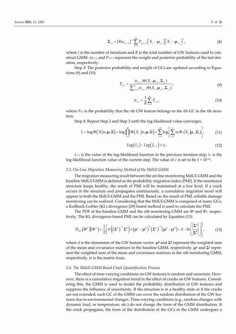
The calibrating process of the MdUI-GMM based crack quantification method is
shown schematically in Figure 1. The process of calibrating PMI with crack using prior
specimens includes three parts:
Part 1 is the baseline MdUI-GMM. GW signal acquisition is performed under time-
varying conditions when the structure is in a healthy state. GW features calculated by
Equation (1) are extracted to construct a GW baseline sample set. After that, the parame-
ters of MdUI-GMM, including weight, mean, and covariance matrix, are trained by an EM
algorithm with a uniform initialization process. Finally, the PDF of the baseline GMM can
be obtained.
Part 2 is online monitoring MdUI-GMM. Once a GW signal is acquired during the
online damage monitoring process, new GW features can be obtained, and the GW feature
sample set is updated first. The updating rule is called first in and first out which means
that the new feature is added to be the last (newest) feature and the first (oldest) feature
is removed. Hence, the number of GW features in the GW feature sample set is consistent.
Then, the parameters of monitoring GMM are trained by an EM algorithm with a uniform
initialization process. Finally, the PDF of monitoring GMM can be obtained.
Part 3 is crack quantification calibration. When a certain number of load cycles is
reached, the fatigue test is paused to measure the crack length using an electron micro-
scope and scale lines on one surface of the specimen. After crack length measurement is
completed, fatigue testing is resumed. By calculating KL divergence between the baseline
GMM in part 1 and the monitoring GMM in part 2, PMI can be obtained. Finally, in com-
bination with the measured crack length, a calibration between PMI and crack length can
be performed.
Figure 1. The process of calibrating probability migration index (PMI) with crack length using
prior specimens.
Sensors 2021, 21, 1283 7 of 20
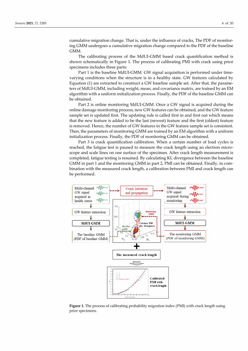
The process of online crack quantification of the new specimen is shown schemati-
cally in Figure 2. Under time-varying conditions, the GW features of the new specimen
are obtained online to construct the online monitoring MdUI-GMM and then PMI can be
calculated. Finally, according to the quantitative calibration relationship between PMI and
crack length in Part 3, the real-time crack length can be calculated directly.
Figure 2. Online crack quantification of the new specimen.
3. Validation on the Notched Specimen of an Aircraft Spar under Fatigue Load
In this section, the fatigue test of notched specimens of an aircraft spar is introduced.
Then, the multi-channel GW features acquired under dynamic load are given and dis-
cussed. After that, crack quantitative calibration results of prior specimens by the MdUI-
GMM, and monitoring results are shown.
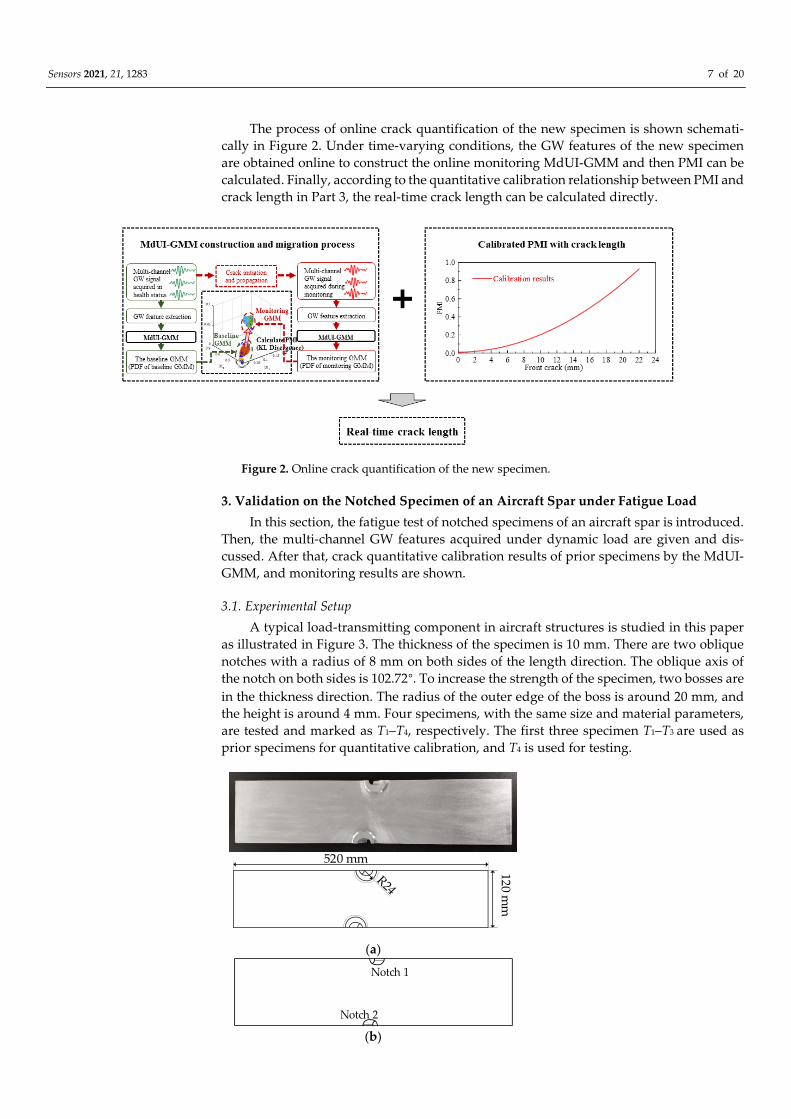
3.1. Experimental Setup
A typical load-transmitting component in aircraft structures is studied in this paper
as illustrated in Figure 3. The thickness of the specimen is 10 mm. There are two oblique
notches with a radius of 8 mm on both sides of the length direction. The oblique axis of
the notch on both sides is 102.72°. To increase the strength of the specimen, two bosses are
in the thickness direction. The radius of the outer edge of the boss is around 20 mm, and
the height is around 4 mm. Four specimens, with the same size and material parameters,
are tested and marked as T1–T4, respectively. The first three specimen T1–T3 are used as
prior specimens for quantitative calibration, and T4 is used for testing.
520 mm
120 m
m
(a)
Notch 1
Notch 2
(b)
Sensors 2021, 21, 1283 8 of 20
(c)
Figure 3. The geometry of the specimen. (a) Front view. (b) Back view. (c) Side view.
The material of the specimen is aluminum alloy 7A04 T7351. Table 1 lists the mechan-
ical properties of aluminum alloy 7A04.
Table 1. The mechanical properties of 7A04.
Material Yield Strength (MPa) Young Modulus (GPa) Tensile Strength (MPa)
7A04 420 70 530
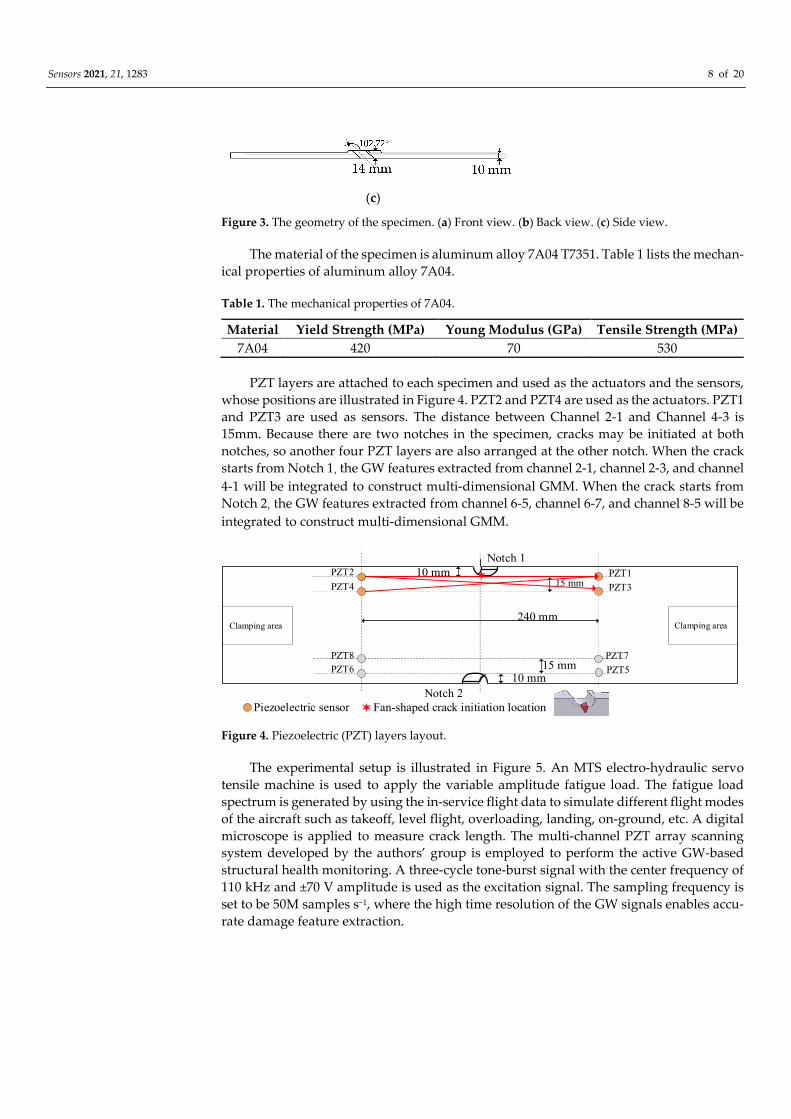
PZT layers are attached to each specimen and used as the actuators and the sensors,
whose positions are illustrated in Figure 4. PZT2 and PZT4 are used as the actuators. PZT1
and PZT3 are used as sensors. The distance between Channel 2-1 and Channel 4-3 is
15mm. Because there are two notches in the specimen, cracks may be initiated at both
notches, so another four PZT layers are also arranged at the other notch. When the crack
starts from Notch 1, the GW features extracted from channel 2-1, channel 2-3, and channel
4-1 will be integrated to construct multi-dimensional GMM. When the crack starts from
Notch 2, the GW features extracted from channel 6-5, channel 6-7, and channel 8-5 will be
integrated to construct multi-dimensional GMM.
Notch 2
Notch 1
10 mm
10 mm15 mm
Piezoelectric sensor
Clamping areaClamping area240 mm
PZT1
PZT3
PZT2
PZT4
15 mmPZT7
PZT5
PZT8
PZT6
Fan-shaped crack initiation location
Figure 4. Piezoelectric (PZT) layers layout.
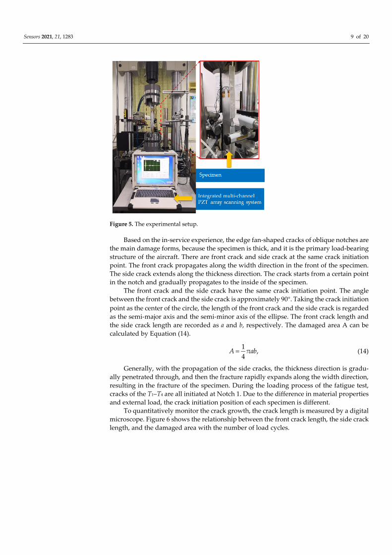
The experimental setup is illustrated in Figure 5. An MTS electro-hydraulic servo
tensile machine is used to apply the variable amplitude fatigue load. The fatigue load
spectrum is generated by using the in-service flight data to simulate different flight modes
of the aircraft such as takeoff, level flight, overloading, landing, on-ground, etc. A digital
microscope is applied to measure crack length. The multi-channel PZT array scanning
system developed by the authors’ group is employed to perform the active GW-based
structural health monitoring. A three-cycle tone-burst signal with the center frequency of
110 kHz and ±70 V amplitude is used as the excitation signal. The sampling frequency is
set to be 50M samples s−1, where the high time resolution of the GW signals enables accu-
rate damage feature extraction.
Sensors 2021, 21, 1283 9 of 20
Figure 5. The experimental setup.
Based on the in-service experience, the edge fan-shaped cracks of oblique notches are
the main damage forms, because the specimen is thick, and it is the primary load-bearing
structure of the aircraft. There are front crack and side crack at the same crack initiation
point. The front crack propagates along the width direction in the front of the specimen.
The side crack extends along the thickness direction. The crack starts from a certain point
in the notch and gradually propagates to the inside of the specimen.
The front crack and the side crack have the same crack initiation point. The angle
between the front crack and the side crack is approximately 90°. Taking the crack initiation
point as the center of the circle, the length of the front crack and the side crack is regarded
as the semi-major axis and the semi-minor axis of the ellipse. The front crack length and
the side crack length are recorded as a and b, respectively. The damaged area A can be
calculated by Equation (14).
1
,4
A πab (14)
Generally, with the propagation of the side cracks, the thickness direction is gradu-
ally penetrated through, and then the fracture rapidly expands along the width direction,
resulting in the fracture of the specimen. During the loading process of the fatigue test,
cracks of the T1–T4 are all initiated at Notch 1. Due to the difference in material properties
and external load, the crack initiation position of each specimen is different.
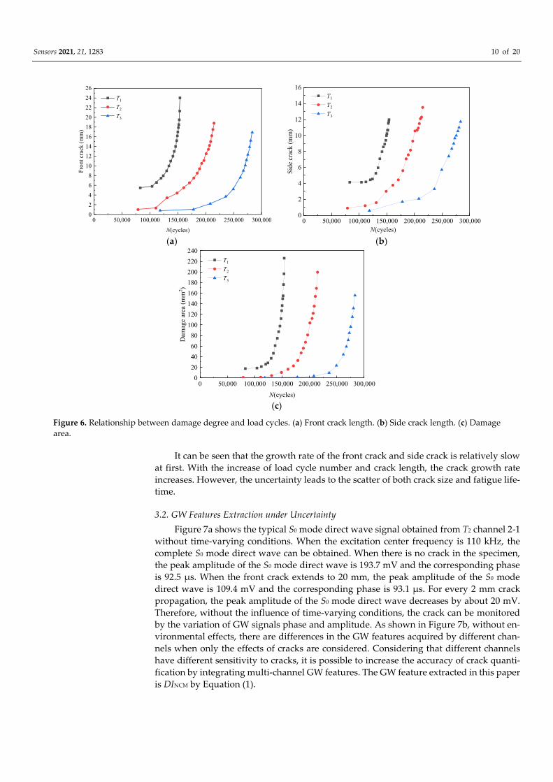
To quantitatively monitor the crack growth, the crack length is measured by a digital
microscope. Figure 6 shows the relationship between the front crack length, the side crack
length, and the damaged area with the number of load cycles.
Sensors 2021, 21, 1283 10 of 20
(a) (b)
(c)
Figure 6. Relationship between damage degree and load cycles. (a) Front crack length. (b) Side crack length. (c) Damage
area.
It can be seen that the growth rate of the front crack and side crack is relatively slow
at first. With the increase of load cycle number and crack length, the crack growth rate
increases. However, the uncertainty leads to the scatter of both crack size and fatigue life-
time.
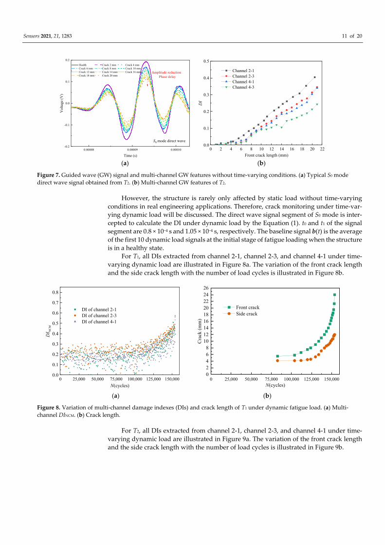
3.2. GW Features Extraction under Uncertainty
Figure 7a shows the typical S0 mode direct wave signal obtained from T2 channel 2-1
without time-varying conditions. When the excitation center frequency is 110 kHz, the
complete S0 mode direct wave can be obtained. When there is no crack in the specimen,
the peak amplitude of the S0 mode direct wave is 193.7 mV and the corresponding phase
is 92.5 μs. When the front crack extends to 20 mm, the peak amplitude of the S0 mode
direct wave is 109.4 mV and the corresponding phase is 93.1 μs. For every 2 mm crack
propagation, the peak amplitude of the S0 mode direct wave decreases by about 20 mV.
Therefore, without the influence of time-varying conditions, the crack can be monitored
by the variation of GW signals phase and amplitude. As shown in Figure 7b, without en-
vironmental effects, there are differences in the GW features acquired by different chan-
nels when only the effects of cracks are considered. Considering that different channels
have different sensitivity to cracks, it is possible to increase the accuracy of crack quanti-
fication by integrating multi-channel GW features. The GW feature extracted in this paper
is DINCM by Equation (1).
0 50,000 100,000 150,000 200,000 250,000 300,0000
2
4
6
8
10
12
14
16
18
20
22
24
26
Fro
nt
crac
k (
mm
)
N(cycles)
T1
T2
T3
0 50,000 100,000 150,000 200,000 250,000 300,0000
2
4
6
8
10
12
14
16
Sid
e cr
ack (
mm
)
N(cycles)
T1
T2
T3
0 50,000 100,000 150,000 200,000 250,000 300,0000
20
40
60
80
100
120
140
160
180
200
220
240
Dam
age
area
(m
m2 )
N(cycles)
T1
T2
T3
Sensors 2021, 21, 1283 11 of 20
(a) (b)
Figure 7. Guided wave (GW) signal and multi-channel GW features without time-varying conditions. (a) Typical S0 mode
direct wave signal obtained from T2. (b) Multi-channel GW features of T2.
However, the structure is rarely only affected by static load without time-varying
conditions in real engineering applications. Therefore, crack monitoring under time-var-
ying dynamic load will be discussed. The direct wave signal segment of S0 mode is inter-
cepted to calculate the DI under dynamic load by the Equation (1). t0 and t1 of the signal
segment are 0.8 × 10⁻⁴ s and 1.05 × 10⁻⁴ s, respectively. The baseline signal b(t) is the average
of the first 10 dynamic load signals at the initial stage of fatigue loading when the structure
is in a healthy state.
For T1, all DIs extracted from channel 2-1, channel 2-3, and channel 4-1 under time-
varying dynamic load are illustrated in Figure 8a. The variation of the front crack length
and the side crack length with the number of load cycles is illustrated in Figure 8b.
(a) (b)
Figure 8. Variation of multi-channel damage indexes (DIs) and crack length of T1 under dynamic fatigue load. (a) Multi-
channel DINCM. (b) Crack length.
For T2, all DIs extracted from channel 2-1, channel 2-3, and channel 4-1 under time-
varying dynamic load are illustrated in Figure 9a. The variation of the front crack length
and the side crack length with the number of load cycles is illustrated in Figure 9b.
0.00008 0.00009 0.00010-0.2
-0.1
0.0
0.1
0.2V
olta
ge (
V)
Time (s)
Health Crack 2 mm Crack 4 mm Crack 6 mm Crack 8 mm Crack 10 mm Crack 12 mm Crack 14 mm Crack 16 mm
Crack 18 mm Crack 20 mmAmplitude reduction Phase delay
S0 mode direct wave
0 2 4 6 8 10 12 14 16 18 20 220.0
0.1
0.2
0.3
0.4
0.5
DI
Front crack length (mm)
Channel 2-1 Channel 2-3 Channel 4-1 Channel 4-3
0 25,000 50,000 75,000 100,000 125,000 150,0000.0
0.1
0.2
0.3
0.4
0.5
0.6
0.7
0.8
DI of channel 2-1 DI of channel 2-3 DI of channel 4-1
DI N
CM
N(cycles)
0 25,000 50,000 75,000 100,000 125,000 150,0000
2
4
6
8
10
12
14
16
18
20
22
24
26
Cra
ck (
mm
)
N(cycles)
Front crack Side crack
Sensors 2021, 21, 1283 12 of 20
(a) (b)
Figure 9. Variation of multi-channel DIs and crack length of T2 under dynamic fatigue load. (a) Multi-channel DINCM. (b)
Crack length.
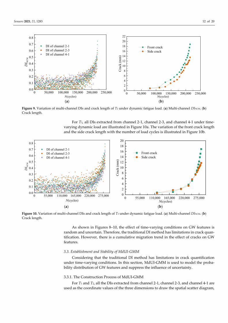
For T3, all DIs extracted from channel 2-1, channel 2-3, and channel 4-1 under time-
varying dynamic load are illustrated in Figure 10a. The variation of the front crack length
and the side crack length with the number of load cycles is illustrated in Figure 10b.
(a) (b)
Figure 10. Variation of multi-channel DIs and crack length of T3 under dynamic fatigue load. (a) Multi-channel DINCM. (b)
Crack length.
As shown in Figures 8–10, the effect of time-varying conditions on GW features is
random and uncertain. Therefore, the traditional DI method has limitations in crack quan-
tification. However, there is a cumulative migration trend in the effect of cracks on GW
features.
3.3. Establishment and Stability of MdUI-GMM
Considering that the traditional DI method has limitations in crack quantification
under time-varying conditions. In this section, MdUI-GMM is used to model the proba-
bility distribution of GW features and suppress the influence of uncertainty.
3.3.1. The Construction Process of MdUI-GMM
For T1 and T2, all the DIs extracted from channel 2-1, channel 2-3, and channel 4-1 are
used as the coordinate values of the three dimensions to draw the spatial scatter diagram,
0 50,000 100,000 150,000 200,000 250,0000.0
0.1
0.2
0.3
0.4
0.5
0.6
0.7
0.8
DI of channel 2-1 DI of channel 2-3 DI of channel 4-1
DI N
CM
N(cycles)0 50,000 100,000 150,000 200,000 250,000
0
2
4
6
8
10
12
14
16
18
20
22
Cra
ck (
mm
)
N(cycles)
Front crack Side crack
0 55,000 110,000 165,000 220,000 275,0000.0
0.1
0.2
0.3
0.4
0.5
0.6
0.7
0.8
DI of channel 2-1 DI of channel 2-3 DI of channel 4-1
DI N
CM
N(cycles)0 55,000 110,000 165,000 220,000 275,000
0
2
4
6
8
10
12
14
16
18
20
Cra
ck (
mm
)
N(cycles)
Front crack Side crack
Sensors 2021, 21, 1283 13 of 20
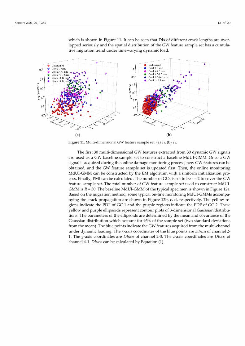
which is shown in Figure 11. It can be seen that DIs of different crack lengths are over-
lapped seriously and the spatial distribution of the GW feature sample set has a cumula-
tive migration trend under time-varying dynamic load.
(a) (b)
Figure 11. Multi-dimensional GW feature sample set. (a) T1. (b) T2.
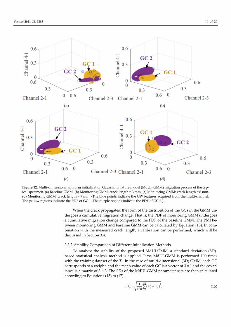
The first 30 multi-dimensional GW features extracted from 30 dynamic GW signals
are used as a GW baseline sample set to construct a baseline MdUI-GMM. Once a GW
signal is acquired during the online damage monitoring process, new GW features can be
obtained, and the GW feature sample set is updated first. Then, the online monitoring
MdUI-GMM can be constructed by the EM algorithm with a uniform initialization pro-
cess. Finally, PMI can be calculated. The number of GCs is set to be c = 2 to cover the GW
feature sample set. The total number of GW feature sample set used to construct MdUI-
GMM is R = 30. The baseline MdUI-GMM of the typical specimen is shown in Figure 12a.
Based on the migration method, some typical on-line monitoring MdUI-GMMs accompa-
nying the crack propagation are shown in Figure 12b, c, d, respectively. The yellow re-
gions indicate the PDF of GC 1 and the purple regions indicate the PDF of GC 2. These
yellow and purple ellipsoids represent contour plots of 3-dimensional Gaussian distribu-
tions. The parameters of the ellipsoids are determined by the mean and covariance of the
Gaussian distribution which account for 95% of the sample set (two standard deviations
from the mean). The blue points indicate the GW features acquired from the multi-channel
under dynamic loading. The x-axis coordinates of the blue points are DINCM of channel 2-
1. The y-axis coordinates are DINCM of channel 2-3. The z-axis coordinates are DINCM of
channel 4-1. DINCM can be calculated by Equation (1).
Sensors 2021, 21, 1283 14 of 20
Figure 12. Multi-dimensional uniform initialization Gaussian mixture model (MdUI- GMM) migration process of the typ-
ical specimen. (a) Baseline GMM. (b) Monitoring GMM: crack length = 3 mm. (c) Monitoring GMM: crack length = 6 mm.
(d) Monitoring GMM: crack length = 9 mm. (The blue points indicate the GW features acquired from the multi-channel.
The yellow regions indicate the PDF of GC 1. The purple regions indicate the PDF of GC 2.).
When the crack propagates, the form of the distribution of the GCs in the GMM un-
dergoes a cumulative migration change. That is, the PDF of monitoring GMM undergoes
a cumulative migration change compared to the PDF of the baseline GMM. The PMI be-
tween monitoring GMM and baseline GMM can be calculated by Equation (13). In com-
bination with the measured crack length, a calibration can be performed, which will be
discussed in Section 3.4.
3.3.2. Stability Comparison of Different Initialization Methods
To analyze the stability of the proposed MdUI-GMM, a standard deviation (SD)-
based statistical analysis method is applied. First, MdUI-GMM is performed 100 times
with the training dataset of the T1. In the case of multi-dimensional (3D) GMM, each GC
corresponds to a weight, and the mean value of each GC is a vector of 3 × 1 and the covar-
iance is a matrix of 3 × 3. The SDs of the MdUI-GMM parameter sets are then calculated
according to Equations (15) to (17).
100 2
1
1,
100i
w c ci
SD w w (15)
Sensors 2021, 21, 1283 15 of 20
i
μ c j c jj i
SD μ μ
3 100 2
, ,1 1
1 1,
3 100 (16)
i
c kj c kjk j i
SD
3 3 100 2
, ,1 1 1
1 1,
9 100 (17)
where c represents the cth GC, c = 1, C. where cw , ,1c , and ,11 c are the average of
weight, mean vector, and covariance matrix, respectively, of the cth component among all
of the 100 parameters sets of MdUI-GMM. i represents the ith modeling process, i = 1, 2,
…, 100.
Table 2 shows the calculated SD of a uniform initialization process. The number of
GCs is set to be C = 2 to cover the GW feature sample set. It is observed that the values of
SD are all less than 10−15, which can be considered to be zero. Hence, it can be concluded
that the modeling results of the MdUI-GMM are always stable.
Table 2. Standard deviation (SD) of a uniform initialization process performing 100 times.
Different States of Structure SDw SDμ SDΣ
Baseline GC 1 9.9920 × 10⁻¹⁷ 4.1633 × 10⁻¹⁸ 5.0963 × 10⁻²¹
GC 2 0 3.7035 × 10⁻¹⁸ 6.8779 × 10⁻¹⁹
1–2 mm GC 1 0 1.3878 × 10⁻¹⁸ 9.4567 × 10⁻²⁰
GC 2 2.7756 × 10⁻¹⁸ 2.8343 × 10⁻¹⁸ 7.1866 × 10⁻²⁰
2–4 mm GC 1 1.2212 × 10⁻¹⁶ 1.5266 × 10⁻¹⁷ 8.2030 × 10⁻²⁰
GC 2 1.1102 × 10⁻¹⁶ 3.0687 × 10⁻¹⁸ 4.3368 × 10⁻²⁰
4–6 mm GC 1 4.4409 × 10⁻¹⁷ 1.1102 × 10⁻¹⁷ 5.1575 × 10⁻²⁰
GC 2 9.9920 × 10⁻¹⁷ 4.6623 × 10⁻¹⁸ 1.1132 × 10⁻¹⁹
Table 3 shows the calculated SD of a k-means initialization process. The number of
GCs is set to be C = 2 to cover the GW feature sample set. It is observed that the values of
SD are higher than those of the MdUI-GMM, which means that the k-means initialization
method is relatively less stable than the uniform initialization method.
Table 3. SD of a k-means initialization process performing 100 times.
Different States of Structure SDw SDμ SDΣ
Baseline GC 1 0.0235 0.0162 5.0064 × 10⁻⁵
GC 2 0.0206 0.0049 1.7724 × 10⁻⁵
1–2 mm GC 1 0.0090 0.0018 2.6628 × 10⁻⁵
GC 2 0.0090 3.4787 × 10⁻⁴ 2.1773 × 10⁻⁵
2–4 mm GC 1 0.0224 0.0027 2.2470 × 10⁻⁵
GC 2 0.0224 0.0015 2.5271 × 10⁻⁵
4–6 mm GC 1 0.0249 0.0037 3.5035 × 10⁻⁵
GC 2 0.0249 9.0958 × 10⁻⁴ 2.3603 × 10⁻⁵
3.4. Calibration Between PMI and Crack Length Using Prior Specimens
The first three specimen T1–T3 are used as prior samples for quantitative calibration,
and T4 is used for testing. For T1–T3, the GW features of channel 2-1, channel 2-3, and
channel 4-1 are fused to construct MdUI-GMM. During the monitoring process, PMI be-
tween monitoring MdUI-GMM and baseline MdUI-GMM is calculated to realize quanti-
tative calibration of front crack length. The variation of PMIs with the length of the front
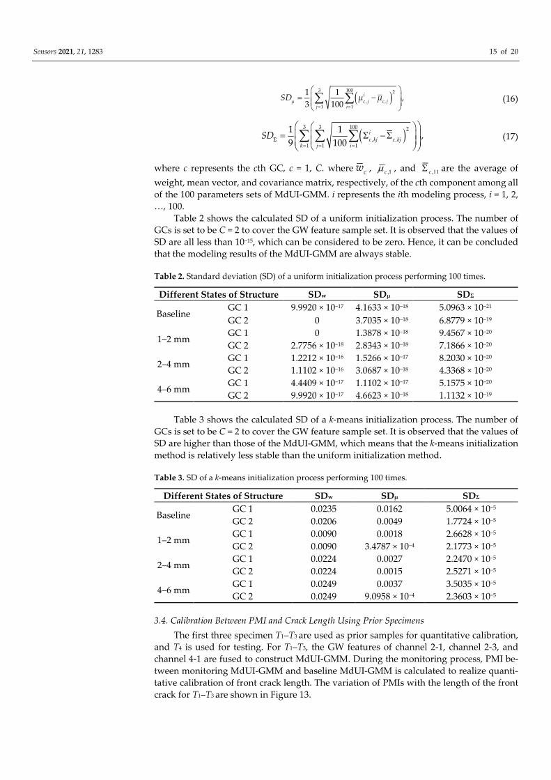
crack for T1–T3 are shown in Figure 13.
Sensors 2021, 21, 1283 16 of 20
Figure 13. Variations of PMI with front crack length.
For T1–T3, the relationship between PMI and crack length is smoothed by a second-
order polynomial and then averaged. After that, the quantitative calibration relationship
between PMI and the front crack length is established.
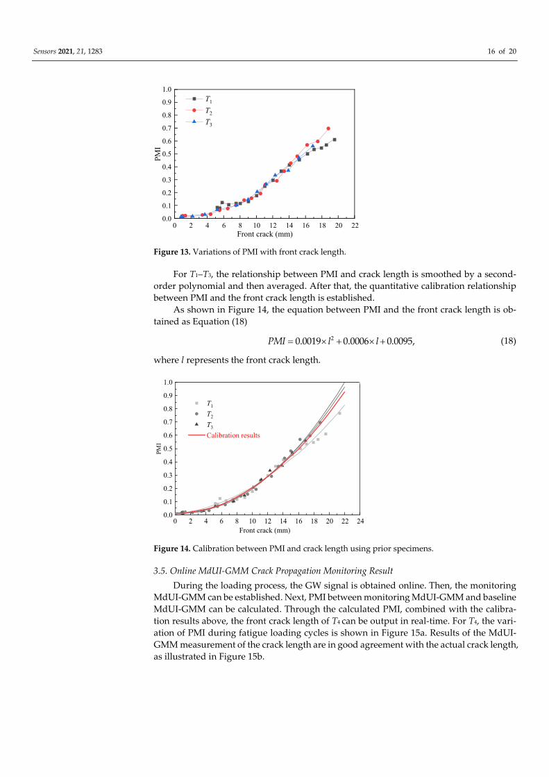
As shown in Figure 14, the equation between PMI and the front crack length is ob-
tained as Equation (18)
20.0019 0. ,0006 0.0095PMI l l (18)
where l represents the front crack length.
Figure 14. Calibration between PMI and crack length using prior specimens.
3.5. Online MdUI-GMM Crack Propagation Monitoring Result
During the loading process, the GW signal is obtained online. Then, the monitoring
MdUI-GMM can be established. Next, PMI between monitoring MdUI-GMM and baseline
MdUI-GMM can be calculated. Through the calculated PMI, combined with the calibra-
tion results above, the front crack length of T4 can be output in real-time. For T4, the vari-
ation of PMI during fatigue loading cycles is shown in Figure 15a. Results of the MdUI-
GMM measurement of the crack length are in good agreement with the actual crack length,
as illustrated in Figure 15b.
0 2 4 6 8 10 12 14 16 18 20 220.0
0.1
0.2
0.3
0.4
0.5
0.6
0.7
0.8
0.9
1.0
PM
I
Front crack (mm)
T1
T2
T3
0 2 4 6 8 10 12 14 16 18 20 22 240.0
0.1
0.2
0.3
0.4
0.5
0.6
0.7
0.8
0.9
1.0
T1
T2
T3
Calibration results
PM
I
Front crack (mm)
Sensors 2021, 21, 1283 17 of 20
(a) (b)
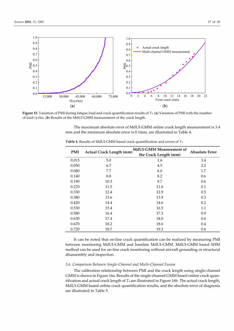
Figure 15. Variation of PMI during fatigue load and crack quantification results of T4. (a) Variation of PMI with the number
of load cycles. (b) Results of the MdUI-GMM measurement of the crack length.
The maximum absolute error of MdUI-GMM online crack length measurement is 3.4
mm and the minimum absolute error is 0.1mm, are illustrated in Table 4.
Table 4. Results of MdUI-GMM based crack quantification and errors of T4.
PMI Actual Crack Length (mm) MdUI-GMM Measurement of
the Crack Length (mm) Absolute Error
0.015 5.0 1.6 3.4
0.050 6.7 4.5 2.2
0.080 7.7 6.0 1.7
0.140 8.8 8.2 0.6
0.190 10.3 9.7 0.6
0.270 11.5 11.6 0.1
0.330 12.4 12.9 0.5
0.380 13.6 13.9 0.3
0.420 14.4 14.6 0.2
0.530 15.4 16.5 1.1
0.580 16.4 17.3 0.9
0.630 17.4 18.0 0.6
0.670 18.2 18.6 0.4
0.720 18.7 19.3 0.6
It can be noted that on-line crack quantification can be realized by measuring PMI
between monitoring MdUI-GMM and baseline MdUI-GMM. MdUI-GMM based SHM
method can be used for on-line crack monitoring without aircraft grounding or structural
disassembly and inspection.
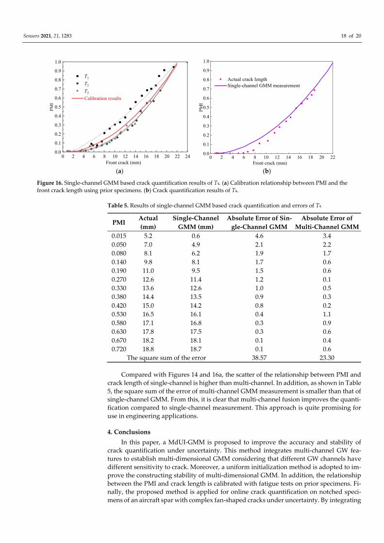
3.6. Comparison Between Single-Channel and Multi-Channel Fusion
The calibration relationship between PMI and the crack length using single-channel
GMM is shown in Figure 16a. Results of the single-channel GMM based online crack quan-
tification and actual crack length of T4 are illustrated in Figure 16b. The actual crack length,
MdUI-GMM based online crack quantification results, and the absolute error of diagnosis
are illustrated in Table 5.
15,000 30,000 45,000 60,000 75,0000.0
0.1
0.2
0.3
0.4
0.5
0.6
0.7
0.8
0.9
1.0
PM
I
N(cycles)
0 2 4 6 8 10 12 14 16 18 20 220.0
0.1
0.2
0.3
0.4
0.5
0.6
0.7
0.8
0.9
1.0
PM
I
Front crack (mm)
Actual crack length Multi-channel GMM measurement
Sensors 2021, 21, 1283 18 of 20
(a) (b)
Figure 16. Single-channel GMM based crack quantification results of T4. (a) Calibration relationship between PMI and the
front crack length using prior specimens. (b) Crack quantification results of T4.
Table 5. Results of single-channel GMM based crack quantification and errors of T4.
PMI Actual
(mm)
Single-Channel
GMM (mm)
Absolute Error of Sin-
gle-Channel GMM
Absolute Error of
Multi-Channel GMM
0.015 5.2 0.6 4.6 3.4
0.050 7.0 4.9 2.1 2.2
0.080 8.1 6.2 1.9 1.7
0.140 9.8 8.1 1.7 0.6
0.190 11.0 9.5 1.5 0.6
0.270 12.6 11.4 1.2 0.1
0.330 13.6 12.6 1.0 0.5
0.380 14.4 13.5 0.9 0.3
0.420 15.0 14.2 0.8 0.2
0.530 16.5 16.1 0.4 1.1
0.580 17.1 16.8 0.3 0.9
0.630 17.8 17.5 0.3 0.6
0.670 18.2 18.1 0.1 0.4
0.720 18.8 18.7 0.1 0.6
The square sum of the error 38.57 23.30
Compared with Figures 14 and 16a, the scatter of the relationship between PMI and
crack length of single-channel is higher than multi-channel. In addition, as shown in Table
5, the square sum of the error of multi-channel GMM measurement is smaller than that of
single-channel GMM. From this, it is clear that multi-channel fusion improves the quanti-
fication compared to single-channel measurement. This approach is quite promising for
use in engineering applications.
4. Conclusions
In this paper, a MdUI-GMM is proposed to improve the accuracy and stability of
crack quantification under uncertainty. This method integrates multi-channel GW fea-
tures to establish multi-dimensional GMM considering that different GW channels have
different sensitivity to crack. Moreover, a uniform initialization method is adopted to im-
prove the constructing stability of multi-dimensional GMM. In addition, the relationship
between the PMI and crack length is calibrated with fatigue tests on prior specimens. Fi-
nally, the proposed method is applied for online crack quantification on notched speci-
mens of an aircraft spar with complex fan-shaped cracks under uncertainty. By integrating
0 2 4 6 8 10 12 14 16 18 20 22 240.0
0.1
0.2
0.3
0.4
0.5
0.6
0.7
0.8
0.9
1.0
T1
T2
T3
Calibration results
PM
I
Front crack (mm)0 2 4 6 8 10 12 14 16 18 20 22
0.0
0.1
0.2
0.3
0.4
0.5
0.6
0.7
0.8
0.9
1.0
Actual crack length Single-channel GMM measurement
PM
I
Front crack (mm)
Sensors 2021, 21, 1283 19 of 20
the multi-channel GW features, the square sum of the error is reduced from 38.57 to 23.30.
The results show that multi-channel fusion improves the quantification compared to the
single-channel measurement of the crack length. Moreover, the standard deviations of the
MdUI-GMM parameter sets are all less than 10−15, which is much smaller than the tradi-
tional k-means initialization method when performing 100 times. The results show that
the construction results of the uniform initialization GMM are always stable.
Author Contributions: Funding acquisition, S.Y.; Methodology, S.Y. and Q.X.; Validation, S.Y., Q.X;
Writing—original draft, Q.X.; Writing—review and editing, S.Y., Q.X., and T.H. All authors have
read and agreed to the published version of the manuscript.
Funding: This work is sponsored by National Natural Science Foundation of China (Grant
No.51921003, Grant No. 51635008, Grant No. 51905266), Jiangsu Provincial Key Research and De-
velopment Program of China (Grant No. BE2018123), Priority Academic Program Development of
Jiangsu Higher Education Institutions of China.
Institutional Review Board Statement: Not applicable.
Informed Consent Statement: Not applicable.
Data Availability Statement: Not applicable.
Conflicts of Interest: The authors declare no conflict of interest.
References
1. Boller, C.; Chang, F.K.; Fujino, Y. Encyclopedia of Structural Health Monitoring; John Wiley & Sons: New York, NY, USA, 2009.
2. Feng, T.; Bekas, D.; Aliabadi, M.H.F. Active Health Monitoring of Thick Composite Structures by Embedded and Surface-
Mounted Piezo Diagnostic Layer. Sensors 2020, 20, 12.
3. Yuan, S.; Ren, Y.; Qiu, L.; Mei, H. A Multi-Response-Based Wireless Impact Monitoring Network for Aircraft Composite Struc-
tures. IEEE Trans. Ind. Electron. 2016, 63, 7712–7722.
4. Wang, Y.; Qiu, L.; Luo, Y.; Ding, R. A stretchable and large-scale guided wave sensor network for aircraft smart skin of structural
health monitoring. Struct. Health Monit. 2019, 1475921719850641. doi:10.1177/1475921719850641.
5. Giurgiutiu, V. Structural Health Monitoring with Piezoelectric Wafer Active Sensors; Academic Press: San Diego, CA, USA, 2014.
6. He, J.; Guan, X.; Peng, T.; Liu, Y.; Saxena, A.; Celaya, J.R.; Goebel, K. A multi-feature integration method for fatigue crack
detection and crack length estimation in riveted lap joints using Lamb waves. Smart Mater. Struct. 2013, 22, 12, doi:10.1088/0964-
1726/22/10/105007.
7. Su, Z.; Zhou, C.; Hong, M.; Cheng, L.; Wang, Q.; Qing, X. Acousto-ultrasonics-based fatigue damage characterization: Linear
versus nonlinear signal features. Mech. Syst. Signal Process. 2014, 45, 225–239, doi:10.1016/j.ymssp.2013.10.017.
8. Qing, X.; Li, W.; Wang, Y.; Sun, H. Piezoelectric Transducer-Based Structural Health Monitoring for Aircraft Applications. Sen-
sors 2019, 19, 545–571, doi:10.3390/s19030545.
9. Liu, Z.; Zhao, X.; Li, J.; He, C.; Wu, B. Obliquely incident EMAT for high-order Lamb wave mode generation based on in-clined
static magnetic field. NDT E Int. 2019, 104, 124–134.
10. Lv, H.; Jiao, J.; Wu, B.; He, C. Numerical Analysis of the Nonlinear Interactions Between Lamb Waves and Mi-crocracks in Plate.
Acta Mech. Solida Sin. 2019, 32, 767–784.
11. Shen, Y.; Cesnik, C.E.S. Nonlinear scattering and mode conversion of Lamb waves at breathing cracks: An efficient nu-merical
approach. Ultrasonics 2019, 94, 202–217.
12. Sobczyk, K.; Spencer, B.F.; Winterstein, S.R. Random Fatigue: From Data to Theory. J. Eng. Mech. 1993, 119, 415–416,
doi:10.1061/(asce)0733-9399(1993)119:2(415).
13. Chen, J.; Yuan, S.; Jin, X. On-line prognosis of fatigue cracking via a regularized particle filter and guided wave monitoring.
Mech. Syst. Signal Process. 2019, 131, 1-17, doi:10.1016/j.ymssp.2019.05.022.
14. Mei, H.; Yuan, S.; Qiu, L.; Zhang, J. Damage evaluation by a guided wave-hidden Markov model based method. Smart Mater.
Struct. 2016, 25, 25021.
15. Chen, J.; Yuan, S.; Wang, H. On-line updating Gaussian process measurement model for crack prognosis using the particle filter.
Mech. Syst. Signal Process. 2020, 140, 106646, doi:10.1016/j.ymssp.2020.106646.
16. Hios, J.D.; Fassois, S.D. A global statistical model based approach for vibration response-only damage detection under var-ious
temperatures: A proof-of-concept study. Mech. Syst. Signal Process. 2014. 49, 77–94.
17. Yuan, S.; Wang, H.; Chen, J. A PZT Based On-Line Updated Guided Wave—Gaussian Process Method for Crack Evaluation.
IEEE Sensors J. 2020, 20, 8204–8212, doi:10.1109/jsen.2019.2960408.
18. Mcnicholas, P.D. Mixture Model-Based Classification; CRC Press: Boca Raton, FL, USA, 2016.

Sensors 2021, 21, 1283 20 of 20
19. Qiu, L.; Fang, F.; Yuan, S. Improved density peak clustering-based adaptive Gaussian mixture model for damage monitoring
in aircraft structures under time-varying conditions. Mech. Syst. Signal Process. 2019, 126, 281–304,
doi:10.1016/j.ymssp.2019.01.034.
20. Chakraborty, D.; Kovvali, N.; Papandreou-Suppappola, A.; Chattopadhyay, A. An adaptive learning damage estimation
method for structural health monitoring. J. Intell. Mater. Syst. Struct. 2014, 26, 125–143, doi:10.1177/1045389X14522531.
21. Banerjee, S.; Qing, X.; Beard, S.; Chang, F.-K. Prediction of Progressive Damage State at the Hot Spots using Statistical Estimation.
J. Intell. Mater. Syst. Struct. 2010, 21, 595–605, doi:10.1177/1045389X10361632.
22. Xu, L.; Yuan, S.; Chen, J.; Ren, Y. Guided Wave-Convolutional Neural Network Based Fatigue Crack Diagnosis of Aircraft
Structures. Sensors 2019, 19, 3567, doi:10.3390/s19163567.
23. Gentle, J.E.; McLachlan, G.J.; Krishnan, T. The EM Algorithm and Extensions. BioM 1998, 54, 395, doi:10.2307/2534032.
24. Yang, J.; He, J.; Guan, X.; Wang, D.; Chen, H.; Zhang, W.; Liu, Y. A probabilistic crack size quantification method using in-situ
Lamb wave test and Bayesian updating. Mech. Syst. Signal Process. 2016, 78, 118–133, doi:10.1016/j.ymssp.2015.06.017.
25. Mitra, M.; Gopalakrishnan, S. Guided wave based structural health monitoring: A review. Smart Mater. Struct. 2016, 25, 053001,
doi:10.1088/0964-1726/25/5/053001.
26. Su, Z.; Ye, L. Identification of Damage Using Lamb Waves; Springer: London, UK, 2009.
27. Torkamani, S.; Roy, S.; E Barkey, M.; Sazonov, E.; Burkett, S.; Kotru, S. A novel damage index for damage identification using
guided waves with application in laminated composites. Smart Mater. Struct. 2014, 23, 95015, doi:10.1088/0964-1726/23/9/095015.
28. Figueiredo, M.A.T.; Jain, A.K. Unsupervised learning of finite mixture models. IEEE Trans. Pattern Anal. Mach. Intell. 2002, 24,
381–396, doi:10.1109/34.990138.
29. Goldberger, J.; Gordon, S.; Greenspan, H. An efficient image similarity measure based on approximations of KL-divergence
between two gaussian mixtures. Proc. ICCV 2003, 1, 487–493, doi:10.1109/iccv.2003.1238387.