Motoristsâ€™ Exposure to Traffic-Related Air Pollution

Bigazzi, Figliozzi, and Clifton 1

1

Motorists’ Exposure to Traffic-Related Air Pollution: 1

Modeling the Effects of Traffic Characteristics 2

3

Alexander Bigazzi (corresponding author) 4

Department of Civil and Environmental Engineering 5

Portland State University 6

P.O. Box 751 7

Portland, OR 97207-0751 8

Email: [email protected] 9

Phone: 503-725-4282 10

Fax: 503-725-5950 11

12

Miguel Figliozzi 13



P.O. Box 751 16

Portland, OR 97207-0751 17


19

Kelly Clifton 20



P.O. Box 751 23

Portland, OR 97207-0751 24


26

27

28

29

30

31

32

33

34

35

Submitted to the 90th Annual Meeting of the Transportation Research Board, January 2011, Washington, D.C. 36

37

38

July 2010 39

40

41

42

43

7,355 words [4,605 + 2 table x250 + 9 figures x250] 44 45


2

ABSTRACT 1 This paper proposes a road-user exposure model that is a function of fundamental traffic characteristics. The 2

model is then applied to a 14-mile congested corridor in Portland, Oregon using real-world traffic data. The 3

modeling results show a wide range of exposures through the corridor over the course of a day and suggest that 4

traffic congestion increases motorists’ exposure to traffic-related pollution. Large peak-period trip exposures are 5

primarily the result of increased exposure durations due to longer travel times. Roadway exposure 6

concentrations (and temporal inhalation rates) also increase during peak periods due to heavy traffic flows and 7

increased marginal emissions rates (though the direct effects of traffic speed on exposure concentrations were 8

small for the case studied). Traffic-induced dispersion increases with higher flows – slightly offsetting the 9

increased roadway emissions during heavy traffic flow. It should be noted that while travel time is the dominant 10

factor in high peak-period exposure, long travel times are driven by traffic characteristics. From a roadway 11

perspective, these results suggest that exposure mitigation should focus on reducing the time spent in the 12

roadway and reducing the volume flow of vehicles on the roadway – while recognizing that these are 13

intertwined travel behaviors. In particular, traveler delay time is less deleterious when spent on low-flow 14

sections than high-flow sections. Finally, individual travelers can greatly reduce their roadway exposure by 15

adjusting their departure time to less congested, lower volume periods. 16

INTRODUCTION 17 Roadway congestion is increasing, and various efforts are underway to reduce its negative impacts (1, 2). Urban 18

freeways carry most of the congestion in the U.S., which has increased more than 50% over the past decade (2). 19

Heavy congestion can increase motor vehicle emissions of air pollutants (3), which progressively degrade urban 20

air quality (4). Because of coincident vehicle and human activity, exposure to traffic-related air pollution 21

increases with urbanization (5). Air pollution in general has been shown to adversely affect human health (6), 22

and exposure to traffic-related pollution in particular is associated with many negative health outcomes (though 23

most causal links are still not conclusive) (7). The transportation microenvironment is an important activity zone 24

as residents of many developed countries spend, on average, more than one hour per day in motor vehicles (8). 25

While increasing levels of urban congestion have been well documented, the effects of congestion on road 26

users’ exposure to pollution have not. 27

Literature reviews by Kaur, Nieuwenhuijsen, & Colvile (9) and Han & Naeher (10) show broad 28

variations in measured pollutant concentrations in different transportation microenvironments. Most past 29

research on road-user exposure is empirical and aggregate because isolating the contributions of individual 30

factors (such as congested traffic characteristics) is difficult and requires a diverse array of measuring 31

equipment. Large-scale exposure models treat journeys as single, static microenvironments, though recent 32

efforts have attempted to model exposure during travel in more detail (8). More detailed models estimate 33

journey exposure using time-weighted averages of air quality concentrations in various sub-microenvironments 34

(i.e. segments of a trip). Modeling of exposure in transportation microenvironments allows experimental control 35

but requires integration of traffic, emissions, air quality, and activity models with significant input data. 36

In light of the health risks posed by human exposure to traffic-related air pollution, this research 37

attempts to model the effects of congested freeway traffic on motorists’ exposure. The central hypothesis tested 38

in this research is that freeway congestion increases drivers’ inhalation of traffic-related pollution. The main 39

contribution of this research is a proposed road-user exposure model that is a function of fundamental traffic 40

state characteristics. The proposed model is estimated and applied for travelers on a freeway in Portland, 41

Oregon. The focus of this research is to enhance our understanding of the impacts of traffic characteristics on 42

travelers’ exposure. The precise estimation of exposure concentrations or mass inhalation rates is outside the 43

scope of this research. This modeling is one step in a larger study effort to quantify the impacts of traffic 44

characteristics on emissions, air quality, and exposure. 45

MODELING ROADWAY EXPOSURE 46 The modeling approach agglomerates sub-microenvironments of roadway segments (i.e. “links”) for a trip on a 47

freeway corridor (which is itself part of a longer journey). The major components included in the model are 48

traffic state (speed and flow), roadway emissions, travel speed, pollutant dispersion, and breathing rate (see 49

Figure 1). The endogenous elements are only those directly affected by traffic congestion and travel mode. The 50

major assumptions and simplifications of the modeling approach are: 51


3

Homogeneous, steady-state traffic states on roadway segments (neglecting traffic state transitions or 1

unsteady traffic conditions) 2

Emissions of counter-flowing vehicle traffic are ignored 3

A steady-state Gaussian line-source dispersion approximation is used 4

Each sub-microenvironment (section of freeway) is modeled by a homogenous set of freeway and 5

environmental characteristics. The traffic state is represented by flow q (in veh/hr) and speed v (in mph). Travel 6

speed is represented as s (in mph). The background concentration Bg is exogenous to the model (though the 7

level of congestion is probably correlated with elevated background concentrations due to peak-period traffic 8

around the city). The pollution emissions rate is E (in grams per vehicle-mile). Although E is determined by 9

many factors, the only endogenous factor is traffic speed; exogenous influences then include vehicle fleet 10

details, fuel formulation, and weather (temperature and humidity). Dispersion of roadway emissions in the plane 11

perpendicular to the roadway is represented by the parameter D in m2/sec, which is controlled by meteorological 12

conditions and traffic-induced turbulence. The penetration of air pollutant concentrations into the vehicle cabin 13

is represented by a unit-less scaling factor P, which is the ratio of in-vehicle concentration to the surrounding 14

concentration. The breathing rate is represented by Ve in m3/hr, which is a function of travel speed for active 15

modes but constant for motor vehicles, and will also vary with individual traveler characteristics. 16

17

18

Figure 1. Components of travel exposure model

Combining these variables, the exposure concentration Ci for a road user in sub-microenvironment i 19

using mode k (in g/m3) is the combined roadway and ambient pollution 20

. (1) 21

The temporal inhalation rate is and the inhalation rate per unit travel distance (in g/mi) is 22

. (2) 23

The total inhalation U (in mass) over a series of roadway segments i is 24

, (3) 25

where Li is the length of roadway traveled in segment i. The average spatial inhalation rate (in g/mi) is 26

, (4) 27

Dispersion D (m2/sec)

Traffic State:Speed v (mi/hr) and

Flow q (veh/hr)

Fuels & Fleet

Exposure Concentration

C (g/m3)

Meteorology

Roadway Emissions E (g/mi)

Mode

Breathing Rate

Ve (m3/hr)

Temporal InhalationItime (g/hr)

Vehicle Penetration P

Travel Speeds (mi/hr)

Traveler Characteristics

Background Conc. Bg (g/m3)

Environment

Road User

Spatial InhalationIdist. (g/mi)

*for active modes

*


4

where is the fractional distance of travel occurring in segment or sub-microenvironment i,

. 1

Finally, the average temporal inhalation rate (in g/hr) is 2

, (5) 3

where

is the fractional time of travel occurring in segment i. Equations 4 and 5 can be 4

simplified by modal characteristics or some of the further assumptions of this analysis, described below. The 5

following sections present methods for estimating the exposure model parameters, which are summarized in 6

Table 1. 7

Table 1: Summary of Model Variables

Variable Symbol Units Endogenous Factors

Emissions Rate E [mass/vehicle-distance] (g/veh-mi) v

Traffic Flow q [veh/time] (veh/hr) Traffic state

Traffic Speed v [distance/time] (mi/hr) Traffic state

Dispersion Parameter D [distance2/time] (m

2/sec) Traffic, wind

Travel Speed s [distance/time] (mi/hr) Mode, v

Breathing Rate Ve [volume/time] (m3/hr) Mode, s

Vehicle Penetration P None Mode

Background Conc. Bg [mass/volume] (g/m3) None

Traffic States 8 For the corridor study below, traffic states (speed and flow) are based on real-world data. We also employ basic 9

traffic flow theory for some analyses. Assuming homogenous traffic conditions on each freeway segment, we 10

can use the fundamental flow-density-speed relationships and first-order macroscopic traffic dynamics described 11

by May (11). Each traffic state is a point on the flow-density (q-k) plane, with a speed corresponding to the slope 12

of the line from the origin (i.e., q=kv). For these relationships q is traffic flow in veh/hr, k is traffic density in 13

veh/mi, and v is traffic speed in mi/hr. Values for constructing the flow-density relationship can be taken from 14

the well-known Highway Capacity Manual (HCM), using the standard basic freeway sections (12). The HCM 15

also describes qualitative level-of-service (LOS) indicators, A-F, based on traffic density thresholds, where LOS 16

F is fully congested (travel demand exceeds roadway capacity). This is a simple but common traffic modeling 17

approach representing homogenous, stationary traffic states on sections of uninterrupted roadway. The 18

macroscopic model represents average conditions – and so is well suited for use with aggregate traffic data and a 19

macroscopic emissions model. 20

Emissions Rates 21 For application with macroscopic traffic characteristics, emissions rates are based on average travel speeds. This 22

approach can capture the average emissions characteristics of congested driving with appropriate driving 23

patterns (13), though the effects of unique microscopic traffic characteristics (such as around toll lanes) are 24

typically not modeled. Emissions-average speed relationships can vary by pollutant (3) and vehicle fleet (i.e. 25

class, age, emissions technology) (14), but a full investigation of different emissions-speed curves is beyond the 26

scope of this paper. 27

For model application average speed-based emissions rates for CO (carbon monoxide), NOx (nitrogen 28

oxides), PM2.5 (particulate matter smaller than 2.5 microns), HC (hydrocarbons), and VOC (volatile organic 29

compounds) are estimated for January 2010 in Portland, Oregon using the MOVES 2010 emissions model (15). 30

These emissions rates are based on a typical daytime mix of vehicle classes on I-5, obtained from the Oregon 31

Department of Transportation (16). Where available, county-specific inputs are used (meteorology, vehicle 32

inspection and maintenance program, fuel formulation), and national averages are used for other model inputs 33


5

(vehicle age distributions). The estimates are for freeway travel only, and the modeled emissions are running 1

exhaust emissions; evaporative, refueling, brake/tire wear, and start emissions are not included. The impacts of 2

particulate resuspension are similarly excluded. 3

The modeled vehicular emissions rates can be combined with traffic states to produce roadway 4

emissions rates (in kilograms per hour per lane-mile of roadway), as shown in Figure 2 for NOx. The roadway 5

emissions rates are plotted as contours on the traffic speed-flow plane, with illustrative real-world traffic states 6

added from I-5NB in Portland, Oregon on January 21, 2010. The traffic states are 5-minute aggregations of 7

dual-loop detector data, and so represent average conditions on a road segment. Roadway emissions rates 8

increase with flow rate, and at very high and very low travel speeds. 9

10

Figure 2. NOx emissions mapped to traffic states, with illustrative real-world traffic data

from I-5NB in Portland, Oregon on January 21, 2010 (5-minute aggregated traffic data)

Breathing Rates 11 Most traffic exposure research accounts for uptake with a breathing/ventilation rate (17-19), though McNabola 12

et al. (20) use a much more complex human respiratory tract model for pollutant absorption. Pollutant uptake 13

can become quite complicated when accounting for factors such personal characteristics, nose vs. mouth 14

breathing, pulse rate, and pollutant compound solubility. Even simple ventilation rate can vary greatly by 15

activity level and personal characteristics (21, 22). A constant, average breathing rate of 0.66 m3/hr is used here 16

for drivers (based on O’Donoghue et al. (23), which also agrees well with Wijnen et al. (24)). Average bicyclist 17

and pedestrian breathing rates can be modeled as linear functions of travel speed, as in McNabola et al. (21). 18

Vehicle Penetration 19 The penetration of pollutants into the vehicle depends primarily on the cabin air exchange rate and is 20

represented by P, a ratio of the in-vehicle concentration to the surrounding concentration. Empirical and 21

modeling studies show that P can vary greatly with vehicle ventilation conditions and cabin particle filters (25-22

27). Clifford, Clarke, & Riffat (28) emphasize the time-lag effect of the vehicle cabin, aside from its potential 23

effects as a barrier. Because the cabin air exchange rate can be affected by speed (17), P could also be a function 24

of the traffic state. Others have suggested that for fine particulates and CO the vehicle shell has no effect – 25

(kg/hr/ln-mi)


6

implying a P value of 1.0 (9). In this research we neglect penetration (P = 1), assuming that any traffic-related 1

effects on P are minimal, and acknowledging that well-sealed cabins with air filters could reduce concentrations 2

levels. 3

Background Concentration 4 In the model formulation background concentration, Bg, includes ambient concentrations and the emissions of 5

counter-flowing and other nearby traffic. These factors are exogenous to this study and the impacts of a 6

congested freeway traffic stream are isolated by excluding background concentrations (Bg = 0). In this way we 7

are modeling only the traffic-related components of total exposure; for pollutants with significant background 8

concentrations, the traffic impacts would be diminished. 9

Dispersion 10 The dispersion parameter D relates pollutant source strength to a concentration at a location of interest, 11

primarily governed by meteorological and traffic conditions. The broad dispersion modeling approach applied 12

here is a semi-infinite continuous line-source Gaussian plume approximation. The technique is essentially the 13

basis of the popular CALINE series of roadway dispersion models (29), and comes from a seminal paper by 14

Benson (30) which accounted for a highly-turbulent roadway mixing zone. Assuming steady-state conditions 15

dominated by cross-road advection, the concentration c at height z can be calculated from the ground-level line 16

source strength Q in mass/length/time, the crosswind speed U, and a statistical approximation of the plume 17

height at some location σz (the standard deviation of the plume density in the vertical direction) 18

. (6) 19

The roadway line source Q is the combined effect of the average vehicle emissions rate and the traffic flow, 20

(in mass/length/time). Combining the other factors to a single variable D, Q can be related to the 21

exposure concentration as , and from a rearrangement of Equation 6, 22

. (7) 23

Assuming a receptor height z of 1m, the remaining step is estimation of the vertical dispersion σz. 24

Research has shown that in addition to local winds, vehicle-induced mechanical turbulence has a significant 25

effect on turbulent dispersion around a roadway (31-33). The effect of the traffic stream on dispersion varies 26

with the traffic speed, traffic density, and size of vehicles. Unfortunately, most roadway dispersion models are 27

intended for use downwind of a roadway, and do not model vehicle-induced turbulence in detail (or at all). 28

When vehicle-induced turbulence is included, it is usually insensitive to traffic characteristics, e.g. (29, 34, 35) – 29

though efforts are under way to incorporate vehicle-induced turbulence in to air dispersion models with more 30

sophistication (36). 31

Because traffic characteristics are the pith of this study, extra effort was made to account for dispersion 32

sensitivity to traffic. The adopted approach to estimating the plume height σz is based on the vehicle wake theory 33

developed by Eskridge, Rao, Thompson, Catalano, and others from wind tunnel studies in the late 1970’s, which 34

is incorporated in the ROADWAY dispersion models (31, 37). The ROADWAY model itself is impractical for 35

this application because it requires microscopic traffic data (individual vehicle paths and speeds), whereas this is 36

a more macroscopic analysis. Vehicle wake theory was also recently used for dispersion modeling in an 37

integrated traffic and air quality simulation (38). 38

The vehicle wake theory is used to estimate the turbulent kinetic energy (TKE) produced by a moving 39

vehicle in a wind field, as illustrated in Figure 3. The TKE behind a vehicle varies with wind speed and 40

direction, vehicle size and drag coefficient, and vehicle speed. For application with macroscopic traffic 41

characteristics in this study, the cumulative roadway TKE from a traffic stream is calculated by assuming equal 42

spacing and distribution of vehicles in each lane and averaging over the roadway. As with other 43

implementations of vehicle wake theory, this assumes independence of turbulent energy plumes. 44


7

1

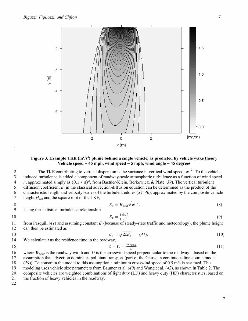
Figure 3. Example TKE (m2/s

2) plume behind a single vehicle, as predicted by vehicle wake theory

Vehicle speed = 45 mph, wind speed = 5 mph, wind angle = 45 degrees

The TKE contributing to vertical dispersion is the variance in vertical wind speed, . To the vehicle-2

induced turbulence is added a component of roadway-scale atmospheric turbulence as a function of wind speed 3

u, approximated simply as , from Bastner-Klein, Berkowicz, & Plate (39). The vertical turbulent 4

diffusion coefficient Ez in the classical advection-diffusion equation can be determined as the product of the 5

characteristic length and velocity scales of the turbulent eddies (34, 40), approximated by the composite vehicle 6

height Hveh and the square root of the TKE, 7

. (8) 8

Using the statistical turbulence relationship 9

(9) 10

from Pasquill (41) and assuming constant Ez (because of steady-state traffic and meteorology), the plume height 11

can then be estimated as 12

(41). (10) 13

We calculate t as the residence time in the roadway, 14

(11) 15

where Wroad is the roadway width and U is the crosswind speed perpendicular to the roadway – based on the 16

assumption that advection dominates pollutant transport (part of the Gaussian continuous line-source model 17

(29)). To constrain the model to this assumption a minimum crosswind speed of 0.5 m/s is assumed. This 18

modeling uses vehicle size parameters from Baumer et al. (40) and Wang et al. (42), as shown in Table 2. The 19

composite vehicles are weighted combinations of light duty (LD) and heavy duty (HD) characteristics, based on 20

the fraction of heavy vehicles in the roadway. 21

22

(m2/s2)


8

Table 2. Assumed vehicle parameters for dispersion estimates

Light Duty Vehicles Heavy Duty Vehicles

Cd, drag coefficient 0.3 0.9

H, vehicle height (m) 1.4 3.5

W, vehicle width (m) 1.8 2.4

L, vehicle length (m) 5.5 22.5

1

The above methodology produces dispersion parameter estimates with changing traffic states as shown 2

in Figure 4, where calculated values of D are plotted on the traffic speed-flow plane, along with solid lines 3

representing HCM theoretical traffic states for free-flow speeds of 60, 65, and 70mph, and dashed lines 4

separating HCM level of service regions (both described above). Higher speeds and flows both increase 5

roadway dispersion, as expected. For generally uncongested traffic (LOS A-E), increasing flows increase 6

dispersion, while increasingly severe levels of congestion in LOS F have lower dispersion estimates. Since D is 7

inversely proportional to traffic-related pollutant concentrations, lower dispersion in heavy congestion will lead 8

to higher roadway concentrations at a given emissions intensity. The dispersion estimates are also moderately 9

sensitive to wind speed and direction, and the fraction of heavy duty vehicles. 10

Like most dispersion modeling this approach is only a rough approximation, and is used as a reasonable 11

estimate of traffic effects while recognizing that short-term concentration values vary widely. Of particular note, 12

this assumes a longitudinally well-mixed roadway air mass, and will likely not accurately represent an idling or 13

extremely slow-moving queue, where the proximity of tailpipes and following vehicles’ air intakes can become 14

a dominant factor (43, 44). 15

16

Figure 4. Roadway dispersion estimates, D (m2/s), with HCM traffic state curves and LOS regions

Wind speed = 5 mph; wind angle = 45 degrees; 3 lanes of 4 m width each

CORRIDOR STUDY 17 To investigate congestion effects on exposure, the exposure model was applied for travelers over 4 days on a 14-18

mile stretch of I-5 NB through Portland, Oregon – see Figure 5. Simulated travelers departed from Milepost 290 19


9

on the southern end of the corridor every 5 minutes from 6am until 8pm on each day of study (January 19-22, 1

2010). Their exposure was modeled over 15 freeway segments (of approximately 1 mile each) up to Milepost 2

305. The freeway segments are delineated by the midpoints between traffic sensors. Traffic conditions (speed 3

and flow) on each link are based on archived inductive dual-loop detector data, as mined from the PORTAL 4

transportation data archive at Portland State University (portal.its.pdx.edu; see (45)). The traffic data were used 5

in 5-minute aggregated form, which has been shown elsewhere to best approximate average freeway travel 6

speeds (46, 47). Although an HOV lane exists at the end of the corridor, it was not used by the simulated 7

travelers (though the emissions/dispersion impacts of the HOV lane vehicles are included). The HD vehicle 8

fraction is based on average vehicle classification data on this section of I-5, with 8.7% HD (16). As local wind 9

data were not available along the freeway, the model used an assumed 5mph wind at 45 degrees clockwise from 10

the direction of traffic flow. Although the local wind speed can have a large effect on pollutant concentrations 11

through dispersion, it is independent of the traffic state and so held constant in the model to investigate traffic 12

effects alone. 13

14

Figure 5. I-5 NB study corridor, (source: (48))

Flow

Direction

Jantzen (307.9)

Marine (307.46)

Delta Park (306.51)

Portland (305.12)

Alberta (304.4)

Going (303.88)

Broadway (302.5)

Morrison (301.09)

Macadam (299.7)

Bertha (297.33)

Multnomah (296.6)

Spring Garden (296.26)

Capital (295.18)

Pacific (293.74)

Haines (293.18)

US217 (292.18)

Upper Boones (291.38)

Lower Boones (290.54)

Nyberg E (289.4)

Stafford W (286.3)

Wilsonville (283.93)

0.70 mi

1.17 mi

1.06 mi

0.62 mi

0.95 mi

1.40 mi

1.40 mi

1.88 mi

1.55 mi

0.54 mi

0.71 mi

1.26 mi

1.00 mi

0.78 mi

0.90 mi

0.82 mi

0.88 mi

2.12 mi

2.74 mi


10

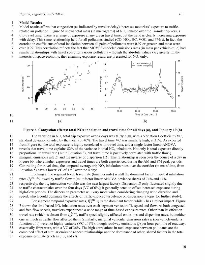
Model Results 1 Model results affirm that congestion (as indicated by traveler delay) increases motorists’ exposure to traffic-2

related air pollution. Figure 6a shows total mass (in micrograms) of NOx inhaled over the 14-mile trip versus 3

trip travel time. There is a range of exposure at any given travel time, but the trend is clearly increasing exposure 4

with delay. This same relationship held for all pollutants studied (CO, NOx, HC, VOC, and PM2.5). In fact, the 5

correlation coefficients of total inhalation between all pairs of pollutants were 0.97 or greater, and most were 6

over 0.99. This correlation reflects the fact that MOVES-modeled emissions rates (in mass per vehicle-mile) had 7

similar relationships with travel speed for various pollutants – though the absolute values vary greatly. In the 8

interests of space economy, the remaining exposure results are presented for NOx only. 9

10

(a) (b) 11

Figure 6. Congestion effects: total NOx inhalation and travel time for all days (a), and January 19 (b)

The variation in NOx total trip exposure over 4 days was fairly high, with a Variation Coefficient (VC, 12

standard deviation divided by the mean) of 40%. The travel time VC was similarly high, at 31%. As expected 13

from Figure 6a, the total exposure is highly correlated with travel time, and a single factor linear ANOVA 14

reveals that travel time explains 82% of the variance in total NOx inhalation. Not only is total exposure directly 15

proportional to travel rate (1/s in Equation 3), but travel time is positively correlated with traffic flow q, 16

marginal emissions rate E, and the inverse of dispersion 1/D. This relationship is seen over the course of a day in 17

Figure 6b, where higher exposures and travel times are both experienced during the AM and PM peak periods. 18

Controlling for travel time, the temporal-average trip NOx inhalation rates over the corridor (in mass/time, from 19

Equation 5) have a lower VC of 17% over the 4 days. 20

Looking at the segment level, travel rate (time per mile) is still the dominant factor in spatial inhalation 21

rates , followed by traffic flow q (multifactor linear ANOVA deviance shares of 74% and 14%, 22

respectively; the v-q interaction variable was the next largest factor). Dispersion D only fluctuated slightly due 23

to traffic characteristics over the four days (VC of 6%); it generally acted to offset increased exposure during 24

high-flow periods. The dispersion parameter will vary more when considering changing wind direction and 25

speed, which could dominate the effects of traffic-induced turbulence on dispersion (a topic for further study). 26

For segment temporal exposure rates, , q is the dominant factor, while v has a minor impact. Figure 27

7 shows the time-based NOx inhalation rates over each segment versus traffic speed and flow. At both congested 28

and free-flow speeds, travelers experienced a wide range of time-based exposure rates. Other than its effect on 29

travel rate (which is absent from ), traffic speed slightly affected emissions and dispersion rates, but neither 30

one as much as traffic flow affected them. Similarly, marginal vehicular emissions rates E (per vehicle-mile, a 31

function of v) were not highly variable (VC of 9%), though roadway emissions Q (per hour per mile of roadway; 32

essentially E*q) were, with a VC of 36%. The high correlations in total exposure between pollutants are the 33

combined effect of similar emissions-speed relationships and the dominance of other, shared factors in the total 34

exposure estimate (such as q, s, and D). 35

15 20 25 30 35 40 45

5

10

15

20

Time Traveled(min)

NO

x in

hale

d (u

g)

0

2

4

6

8

10

12

14

NO

x in

ha

led

(u

g)

08:00 12:00 16:00 20:00

12

14

16

18

20NOx Inhaled (ug)Travel Time (min)

Tra

ve

l T

ime

(m

in)

Time of Day, Jan. 19


11

1

Figure 7. Time-based segment NOx inhalation rates with traffic characteristics

As a further illustration of the impacts of travel time, consider an alternative hypothetical traveler who 2

traverses the same road segments at the same times as the travelers in the congested traffic stream, but at a 3

constant free-flow speed unhindered by other vehicles (a free-flowing HOV lane, for example, where s is 4

independent of v). These travelers have the same exposure concentrations C as the motorists in congestion, but 5

shorter (or equal) exposure durations. Figure 8 compares the total trip inhalations over the course of a day for a 6

traveler in the congested stream and a constant-speed traveler (at 60mph, for 14 minutes total travel time). 7

Although there is a moderate increase in exposure during the day, the extreme exposures during the AM and PM 8

peaks are avoided. The large exposure peaks during peak-period congestion are primarily the result of increased 9

time in the traffic stream (exposure duration), while the influence of traffic on exposure concentrations is 10

secondary. 11

12

Figure 8. Comparison of total trip inhalation for congested and constant-speed (60mph) travelers

0

5

10

15

Departure Time, Jan. 19

NO

x in

ha

led

(u

g)

08:00 12:00 16:00 20:00

Congested travelerConstant-speed traveler


12

The variability in trip exposures is illustrated in Figure 9, where individual trip trajectories are plotted as 1

cumulative mass inhaled versus traveled distance and time. The slopes of these trajectories are the inhalation 2

rates, and we can clearly see the effects of bottlenecks spatially in the first panel, where congestion around miles 3

4 and 8 rapidly increase total exposure for some motorists (both are bottlenecks upstream of major 4

interchanges). High-exposure motorists experience much of their inhalation at isolated locations, while the rest 5

of their trip has a similar slope to that of the motorists not experiencing congestion. From an exposure point of 6

view, there are clearly “hot spots” on the corridor with long travel durations and high traffic flows. 7

8

Figure 9. Trip trajectories in mass inhaled versus distance and time traveled

The second panel in Figure 9 shows the temporal intensity of exposure, and we see that free-flowing 9

trips (around 15 minutes) terminate with much lower total inhalation than longer trips. That said, there was still 10

a wide range of exposures for moderate-delay trips (20-25 minute travel times). Based on the above analysis, the 11

varying slopes in this plot are primarily determined by surrounding traffic flows; a fixed amount of delay is less 12

harmfully experienced on a lower-flow section than a higher-flow section. 13

CONCLUSIONS 14 This paper proposes and applies a road-user exposure model that is a function of fundamental traffic state 15

characteristics. The modeling results of the case study show a wide range of exposures through a freeway 16

corridor over the course of a day and suggest that traffic congestion does increase motorists’ exposure to traffic-17

related pollution. Traffic characteristics affect motorists’ exposure in multiple ways. Large peak-period trip 18

exposures are primarily the result of increased exposure durations due to longer travel times. This is reflected by 19

more moderate traffic impacts on exposure for road users with travel speeds unaffected by the traffic state. 20

Roadway exposure concentrations (and temporal inhalation rates) also increase during peak periods due to 21

heavy traffic flows and increased marginal emissions rates (though the direct effects of traffic speed on exposure 22

concentrations were small for the case studied). Traffic-induced dispersion increases with higher flows – slightly 23

offsetting the increased roadway emissions during heavy traffic flow. 24

It should also be noted that while travel time is the dominant factor in high peak-period exposure, long 25

travel times are driven by traffic characteristics. Excess travel demand volumes increase exposure by causing 26

traveler delay, in addition to increasing roadway emissions through high flows and increased marginal emissions 27

rates. Motorists’ exposure to traffic-related pollution can be mitigated by diverse strategies, including cleaner 28

vehicles and fuels, more efficient roadways, and changing travel behaviors (trips, routes, and modes). From a 29

roadway perspective, these results suggest that the focus should be on reducing the time spent in the roadway 30

and reducing the volume flow of vehicles on the roadway – while recognizing that these are intertwined travel 31

behaviors. In particular, traveler delay time is less deleterious when spent on low-flow sections than high-flow 32

sections. Individual travelers can greatly reduce their roadway exposure by adjusting their departure time to less 33

congested, lower volume periods. 34

0 2 4 6 8 10 12 14

0

2

4

6

8

10

12

14

Cumulative Mass Inhaled vs. Distance

Distance Traveled(mi)

NO

x in

ha

led

(u

g)

0 5 10 15 20 25 30 35

0

2

4

6

8

10

12

14

Cumulative Mass Inhaled vs. Travel Time

Time Traveled(min)

NO

x in

ha

led

(u

g)


13

These results have been presented with respect to departure time, not total trips taken. As such, they 1

represent varying marginal exposure for a motorist, depending on when they enter the corridor. For a population 2

perspective, these would be weighted by travel flows, which would reflect the increased numbers of motorists 3

during peak periods (when most congestion occurs). For a broader picture of the role of congestion in overall 4

exposure we would also need to consider background concentrations and alternative exposure environments, 5

indirect congestion effects on mode choice, routing, and land use, and travel delay effects on time allocation, 6

(such as in Zhang & Batterman (49)). 7

These conclusions are based on the results of a modeling exercise with many assumptions and 8

approximations. Salient weaknesses include the imprecise representation of “stop-and-go” conditions, the use of 9

homogenous, steady traffic states, and the simplified modeling of roadway dispersion. Next steps include in-10

vehicle air quality measurements to validate these results and modeling of other road users such as counter-11

flowing motorists, bicyclists, and pedestrians (on parallel paths). Additionally, continued modeling efforts will 12

investigate exposure effects of seasonal flows, HOV lanes, and local wind conditions. Continued development 13

of mesoscopic roadway dispersion models is another important research path. Finally, we hope to use exposure 14

modeling to estimate the health impacts of congestion – marginally for travelers and cumulatively for the 15

Portland metropolitan region. 16

ACKNOWLEDGMENTS 17 The authors would like to thank for their support of this project: the Oregon Transportation Research and 18

Education Consortium (OTREC) and the U.S. Department of Transportation (through the Eisenhower Graduate 19

Fellowship program). 20

REFERENCES 21

[1] European Conference of Ministers of Transport (ECMT), Managing Urban Traffic Congestion, 22

OECD, Transport Research Center, 2007. 23

[2] Schrank, D. and T. Lomax, “The 2007 urban mobility report,” Texas Transportation Institute, 24

College Station, TX, 2007. 25

[3] Barth, M., G. Scora, and T. Younglove, “Estimating emissions and fuel consumption for different 26

levels of freeway congestion,” Transportation Research Record: Journal of the Transportation 27

Research Board, vol. 1664, 1999, pp. 47–57. 28

[4] Fenger, J., “Urban air quality,” Atmospheric Environment, vol. 33, 1999, pp. 4877–4900. 29

[5] Van Atten, C., M. Brauer, T. Funk, N.L. Gilber, L. Graham, D. Kaden, and others, “Assessing 30

population exposures to motor vehicle exhaust,” Rev Environ Health, vol. 20, 2005, pp. 195–214. 31

[6] Bernstein, J., N. Alexis, C. Barnes, I. Bernstein, J. Bernstein, A. Nel, D. Peden, D. Diaz-Sanchez, 32

S. Tarlo, and P. Williams, “Health effects of air pollution,” The Journal of Allergy and Clinical 33

Immunology, vol. 114, 2004, pp. 1116–1123. 34

[7] Health Effects Institute, Traffic-Related Air Pollution: A Critical Review of the Literature on 35

Emissions, Exposure, and Health Effects, Health Effects Institute, 2010. 36

[8] Gulliver, J. and D.J. Briggs, “Time-space modeling of journey-time exposure to traffic-related air 37

pollution using GIS,” Environmental Research, vol. 97, Jan. 2005, pp. 10-25. 38

[9] Kaur, S., M. Nieuwenhuijsen, and R. Colvile, “Fine particulate matter and carbon monoxide 39

exposure concentrations in urban street transport microenvironments,” Atmospheric Environment, 40

vol. 41, Jul. 2007, pp. 4781-4810. 41

[10] Han, X. and L.P. Naeher, “A review of traffic-related air pollution exposure assessment studies in 42

the developing world,” Environment international, vol. 32, 2006, pp. 106–120. 43

[11] May, Traffic Flow Fundamentals, Prentice Hall, 1989. 44

[12] Transportation Research Board, Highway Capacity Manual, Washington, D.C.: National 45

Research Council, 2000. 46

[13] Smit, R., A.L. Brown, and Y.C. Chan, “Do air pollution emissions and fuel consumption models 47

for roadways include the effects of congestion in the roadway traffic flow?,” Environmental 48


14

Modelling and Software, vol. 23, 2008, pp. 1262–1270. 1

[14] Boulter, P.G., T.J. Barlow, I.S. McCrae, and S. Latham, Emissions factors 2009: Final summary 2

report, UK Department for Transport, 2009. 3

[15] U.S. Environmental Protection Agency (EPA), Motor Vehicle Emission Simulator (MOVES) 2010 4

User's Guide, U.S. EPA, 2009. 5

[16] Oregon Department of Transportation, “Traffic Volumes and Vehicle Classification,” Jul. 2009. 6

[17] Johnson, T., A Guide to Selected Algorithms, Distributions, and Databases Used in Exposure 7

Models Developed by The Office Of Air Quality Planning and Standards, Research Triangle Park, 8

NC: U.S. Environmental Protection Agency, Office of Research and Development, 2002. 9

[18] Nazelle, A.D., D.A. Rodríguez, and D. Crawford-Brown, “The built environment and health: 10

Impacts of pedestrian-friendly designs on air pollution exposure,” Science of The Total 11

Environment, vol. 407, Apr. 2009, pp. 2525-2535. 12

[19] Rank, J., J. Folke, and P. Homann Jespersen, “Differences in cyclists and car drivers exposure to 13

air pollution from traffic in the city of Copenhagen,” Science of the Total Environment, The, vol. 14

279, 2001, pp. 131–136. 15

[20] McNabola, A., B.M. Broderick, and L.W. Gill, “Relative exposure to fine particulate matter and 16

VOCs between transport microenvironments in Dublin: Personal exposure and uptake,” 17

Atmospheric Environment, vol. 42, 2008, pp. 6496–6512. 18

[21] McNabola, A., B.M. Broderick, and L.W. Gill, “Optimal cycling and walking speed for minimum 19

absorption of traffic emissions in the lungs,” Journal of environmental science and health. Part A, 20

Toxic/hazardous substances & environmental engineering, vol. 42, 2007, p. 1999. 21

[22] Zuurbier, M., G. Hoek, P. Hazel, and B. Brunekreef, “Minute ventilation of cyclists, car and bus 22

passengers: an experimental study,” Environmental Health, vol. 8, 2009, p. 48. 23

[23] O'Donoghue, R.T., L.W. Gill, R.J. McKevitt, and B. Broderick, “Exposure to hydrocarbon 24

concentrations while commuting or exercising in Dublin,” Environment international, vol. 33, 25

2007, pp. 1–8. 26

[24] Wijnen, J.H., A.P. Verhoeff, H.W. Jans, and M. Bruggen, “The exposure of cyclists, car drivers 27

and pedestrians to traffic-related air pollutants,” International archives of occupational and 28

environmental health, vol. 67, 1995, pp. 187–193. 29

[25] Chan, A.T. and M.W. Chung, “Indoor-outdoor air quality relationships in vehicle: effect of 30

driving environment and ventilation modes,” Atmospheric Environment, vol. 37, Sep. 2003, pp. 31

3795-3808. 32

[26] Liu, X., H.C. Frey, and Y. Cao, “Estimation of In-Vehicle Concentration and Human Exposure 33

for PM2.5 Based on Near Roadway Ambient Air Quality and Variability in Vehicle Operation,” 34

89th Annual Meeting of the Transportation Research Board, Washington, D.C.: 2010. 35

[27] Zhu, Y., A. Eiguren-Fernandez, W.C. Hinds, and A.H. Miguel, “In-Cabin Commuter Exposure to 36

Ultrafine Particles on Los Angeles Freeways,” Environmental Science & Technology, vol. 41, 37

Apr. 2007, pp. 2138-2145. 38

[28] Clifford, M.J., R. Clarke, and S.B. Riffat, “Drivers' exposure to carbon monoxide in Nottingham, 39

U.K.,” Atmospheric Environment, vol. 31, Apr. 1997, pp. 1003-1009. 40

[29] Benson, P., “A review of the development and application of the CALINE 3 and 4 models,” 41

Atmospheric environment. Part B, Urban atmosphere, vol. 26, 1992, pp. 379–390. 42

[30] Benson, P., “Modifications to the Gaussian vertical dispersion parameter, $\sigma$z, near 43

roadways,” Atmospheric Environment, vol. 16, 1982, pp. 1399–1405. 44

[31] Eskridge, R.E. and S.T. Rao, “Turbulent diffusion behind vehicles: experimentally determined 45

turbulence mixing parameters,” Atmospheric Environment, vol. 20, 1986, pp. 851–860. 46

[32] Kalthoff, N., D. B\äumer, U. Corsmeier, M. Kohler, and B. Vogel, “Vehicle-induced turbulence 47

near a motorway,” Atmospheric Environment, vol. 39, 2005, pp. 5737–5749. 48


15

[33] Rao, K.S., R.L. Gunter, J.R. White, and R.P. Hosker, “Turbulence and dispersion modeling near 1

highways,” Atmospheric Environment, vol. 36, 2002, pp. 4337–4346. 2

[34] Kono, H. and S. Ito, “A micro-scale dispersion model for motor vehicle exhaust gas in urban 3

areas--OMG volume-source model,” Atmospheric Environment. Part B. Urban Atmosphere, vol. 4

24, 1990, pp. 243-251. 5

[35] Held, T., D. Chang, and D. Niemeier, “UCD 2001: An improved model to simulate pollutant 6

dispersion from roadways,” Atmospheric Environment, vol. 37, 2003, pp. 5325–5336. 7

[36] Kanda, I., K. Uehara, Y. Yamao, Y. Yoshikawa, and T. Morikawa, “A wind-tunnel study on 8

exhaust-gas dispersion from road vehicles–Part II: Effect of vehicle queues,” Journal of Wind 9

Engineering and Industrial Aerodynamics, vol. 94, 2006, pp. 659–673. 10

[37] Rao, K.S., “ROADWAY-2: A Model for Pollutant Dispersion near Highways,” Water, Air, & 11

Soil Pollution: Focus, vol. 2, 2002, pp. 261-277. 12

[38] Kim, B., R. Wayson, and G. Fleming, “Development of Traffic Air Quality Simulation Model,” 13

Transportation Research Record: Journal of the Transportation Research Board, vol. 1987, 14

2006, pp. 73-81. 15

[39] Kastner-Klein, P., R. Berkowicz, and E.J. Plate, “Modelling of vehicle-induced turbulence in air 16

pollution studies for streets,” International Journal of Environment and Pollution, vol. 14, 2000, 17

pp. 496–507. 18

[40] Baumer, D., B. Vogel, and F. Fiedler, “A new parameterisation of motorway-induced turbulence 19

and its application in a numerical model,” Atmospheric Environment, vol. 39, 2005, pp. 5750–20

5759. 21

[41] Pasquill, F., Pasquill Atmospheric Diffusion 3ed - Study of the Dispersion of Windborne Material 22

Etc., Ellis Horwood Ltd, Publisher, 1983. 23

[42] Wang, J., T. Chan, C. Cheung, C. Leung, and W. Hung, “Three-dimensional pollutant 24

concentration dispersion of a vehicular exhaust plume in the real atmosphere,” Atmospheric 25

Environment, vol. 40, Jan. 2006, pp. 484-497. 26

[43] Clifford, M.J., R. Clarke, and S.B. Riffat, “Local aspects of vehicular pollution,” Atmospheric 27

Environment, vol. 31, Jan. 1997, pp. 271-276. 28

[44] McNabola, A., B. Broderick, and L. Gill, “The impacts of inter-vehicle spacing on in-vehicle air 29

pollution concentrations in idling urban traffic conditions,” Transportation Research Part D: 30

Transport and Environment, vol. 14, Dec. 2009, pp. 567-575. 31

[45] Bertini, R.L., S. Hansen, A. Byrd, and T. Yin, “Experience implementing a user service for 32

archived intelligent transportation systems data,” Transportation Research Record: Journal of the 33

Transportation Research Board, vol. 1917, 2005, pp. 90–99. 34

[46] Bigazzi, A., H. Siri, and R. Bertini, “Effects of Temporal Data Aggregation on Performance 35

Measures and other ITS Applications,” 89th Annual Meeting of the Transportation Research 36

Board, Washington, D.C.: 2010. 37

[47] Wang, Z. and C. Liu, “An empirical evaluation of the loop detector method for travel time delay 38

estimation,” Journal of Intelligent Transportation Systems, vol. 9, 2005, pp. 161–174. 39

[48] Saberi, M. and R. Bertini, “Beyond Corridor Reliability Measures: Analysis of Freeway Travel 40

Time Reliability at the Segment Level for Hotspot Identification,” 89th Annual Meeting of the 41

Transportation Research Board, Washington, D.C.: 2010. 42

[49] Zhang, K. and S.A. Batterman, “Time allocation shifts and pollutant exposure due to traffic 43

congestion: An analysis using the national human activity pattern survey,” Science of the Total 44

Environment, vol. 407, Oct. 2009, pp. 5493-5500. 45

46

Motoristsâ€™ Exposure to Traffic-Related Air Pollution

Documents

Transcript of Motoristsâ€™ Exposure to Traffic-Related Air Pollution