Motion Control Strategies based on PD Control for a...

International Journal of Computer Applications (0975 – 8887)

Volume 109 – No. 13, January 2015

35

Motion Control Strategies based on PD Control for a

Four Degree-of-Freedom Serial Robotic Manipulator to

Mimic Human Index Finger Articulations

Abhijit Mahapatra CSIR-CMERI,

Durgapur, India.

Kaustav Biswas NIT Durgapur

Durgapur, India.

Amit Kumar CSIR-CMERI,

Durgapur, India.

Avik Chatterjee CSIR-CMERI,

Durgapur, India.

ABSTRACT

The present study is based on motion control of an articulated

model of a human index finger that has been modeled as a

four-degree-of-freedom serial robotic manipulator.

Preliminary studies on position and tracking control have been

carried out by testing various control strategies based on

proportional-derivative (PD) control in a simulation

environment wherein the manipulator has been modeled and

simulated with a certain input signal and responses to various

controllers have been shown. Model free and model based

controllers have been designed simulated using MATLAB®/

Simulink®. Strategies like model free PD control have been

improved upon by introducing auto-tuning and learning

capabilities. A virtual plant modeled using Simmechanics®

toolbox has been set up and used for simulation purposes.

General Terms

Degree of freedom, human hand articulations, serial

manipulators

Keywords

PD Control, Feed-forward Control, Computed Torque

Control, Human Index Finger, Simmechanics

1. INTRODUCTION Since the beginning of humanity‟s quest with robotics and

artificial intelligence, robotic manipulators have been widely

studied, developed and implemented in various fields.

Combined with structural diversity, the different types of

control systems developed over time have enabled the use of

manipulators for a wide variety of tasks ranging from

industrial to domestic. Recently, robotic manipulators are being tested in the field of rehabilitation of patients who have

partially lost the functionality of limb(s). The human hand is a

highly articulated manipulator with a large number of degrees

of freedom. Mimicking the functionality of the human hand

using a machine is an interesting problem of robotic and

control systems research. In the present study, an attempt has

been made to develop an articulated hand model and

subsequently implement various motion control algorithms to

mimic actions like palmer grasping (Fig. 1). The methods

developed can be used to construct a functional wearable

exoskeleton for the human hand or a remotely controlled

robotic hand which may communicate with this exoskeleton,

worn by a human operator, facilitating its use in a variety of

tasks like remote manipulation, physiotherapy etc., thus

broadening the avenue of Human Computer Interaction.

Fig. 1: CAD model of the human hand showing various

joints and associated degrees of freedom

The study has been aided by important concepts presented in

[1], [2] and [3]. Modeling of model free PD controllers has

been very well explained in [4] and [5]. Innovative control

architectures have been presented in [6]. Studies on model

based control techniques like feed-forward (FFD) control and

computed torque (CTC) control have been presented in [7],

[8] and [9]. Further, we have referred to [10], [11] and [12]

for motivation. Commercially available products similar to the

one in this study are the Festo® „Exohand‟, the „Shadow

Dexterous Hand™‟ etc.

The present paper has been categorized into five sections.

Section 2 describes the mechanical and mathematical model

setup for the problem using the Lagrange-Euler formulation

for modeling dynamics of the manipulator. Section 3 presents

the development of various controller strategies for

controlling a single finger modeled as a four degree of

freedom manipulator, with some controllers using the

dynamic model developed in the previous section. Section 4

presents modeling and simulation of the finger manipulator,

which show the response of various control systems to a

specified input signal. Section 5 concludes the paper.



36

[

Re

po

rt

Su

bti

tle

]

2. MODEL OF THE MANIPULATOR

2.1 Mathematical Model The inverse dynamic formulation according to Euler-

Lagrange formulation for a general n-link manipulator is

given by the following equation, as described in [1]:

( ) ( , ) ( ) ( , ) M H G F τq q q q q q q (1)

For the present case, ‘q’ is the generalized co-ordinate, here,

the joint angle; ‘M’ is the 4×4 matrix of link inertias; ‘H’ is

the matrix of Coriolis/centripetal forces and ‘G’ represents the

gravity vector. ‘F’ is the matrix of joint stiffness and damping

terms. ‘τ’ may represent the vector of generalized forces or

torques applied by an actuator.

1 2 3 4T

[ ]q = q q q q (2)

1 2 3 4T

[ ]τ = τ τ τ τ (3)

11 12 13 14

21 22 23 24

31 32 33 34

41 42 43 44

( ) ( ) ( ) ( )

( ) ( ) ( ) ( )

( ) ( ) ( ) ( )

( ) ( ) ( ) ( )

M q M q M q M q

M q M q M q M q

M q M q M q M q

M q M q M q M q

M (4)

1 2 3 4( , ) ( , ) ( , ) ( , ) TH H H HH [ ]= q q q q q q q q (5)

1 2 3 4( ) ( ) ( ) ( ) TG G G GG [ ]= q q q q (6)

1 2 3 4( , ) ( , ) ( , ) ( , ) TF F F FF [ ]= q q q q q q q q (7)

The elements of the „M‟ matrix are of the form: 4

max( , )

T

ik jk j ji

j i k

M Tr

d Ι d (8)

where, Ij represents the Identity matrix of order 4x4, and i,k =

1,2,3,4. „Tr‟ represents the trace of the matrix.

Also,

0 0 11

0

ji j j i

ij

j

j i

j i

T T Q Td

and Qj=Qk=[0 -1 0 0;1 0 0 0;0 0 0 0;0 0 0 0] for a rotary joint

The elements of the „H‟ matrix are of the form:

4 4

1 1

i ikm k m

k m

H h q q

(9)

where

4

max( , , )

Tikm jkm j ji

j i k m

h Tr

d I d , i, k, m=1, 2, 3, 4

0 1 11 1

0 1 11 1

0 ,

j kj j k k i

ij k jijk k k j j i

k

i k j

i j kq

i j i k

T Q T Q Td

d T Q T Q T

where the „aTb‟ terms represent transformation matrices as

obtained from Denavit-Hartenberg formulation as described in

[1, 2]. The terms of the „G‟ matrix are of the form:

4

.T ji j ji j

j i

G m

g d r where i= 1 to 4 (10)

„mj‟ represents the mass of the link j, „rj‟ represents its radius

in case of a cylindrical link and „g‟ represents acceleration due

to gravity = 9.81 m/s2.

Thus the expression for torque applied by actuator at joint p

(neglecting joint stiffness and damping) is obtained by

substituting values of various terms in equation (1):

τ j 4 4

1

Tjk j ji k

j i k

Tr q

d Ι d

4 4 4

1 1

Tjkm j ji k m

j i k m

Tr q q

d Ι d

4

.T jj ji j

j i

m

g d r (11)

If we include joint stiffness and damping terms as terms of the

„F‟ matrix then,

( , )i i i i iF q q d q c q (12)

where „di‟ and „ci‟ terms are stiffness and damping constants

and the „F‟ matrix is added to the overall torque matrix

obtained above. Generally, it is difficult to determine the

exact nature of the terms of this matrix. Here it has been

assumed that ci = qi2 and di = 0.25 ci.

2.2 Mechanical Model The virtual plant model for simulation that has been created in

the Simmechanics® environment of Simulink® and shown in

Section 4 has been constructed using the following inertia

tensor for each link.

Ij=[(-jIxx+jIyy+

jIzz)/2 jIxy jIxz mj jx ; jIxy (

jIxx-jIyy+

jIzz)/2 jIyz

mjӯj; jIxz

jIyz (jIxx+

jIyy-jIzz)/2 mj jz ; mj jx mjӯj mj jz mj] (13)

where the jIxy, jIyz,

jIxz terms represent cross products of inertia

and jIxx, jIyy,

jIzz terms represent moment of inertia with respect

to the x, y and z axis respectively; mj is the mass of the link j.

In a right handed coordinate system {x y z}, Ixx=∫(y2+z2)dm;

Ixy=∫xy dm and so on.

A simplified model taking into account stiffness and

damping effects at each joint has been shown in Fig. 2(a) and

free body diagrams for the links have been shown in Fig. 2(b).

Here the joint angles have been represented by „θi‟ terms and

actuator torques as „τMi‟ terms.

(a)



37

Fig.2: (a) Simplified physical model showing each link as a

line and joints as cylinders with stiffness and damping

terms; (b) Free body diagrams of all the links with

actuator torques indicated

3. CONTROL SYSTEM FOR THE

MANIPULATOR Various effective control strategies for robotic manipulators

have been reported. These include the conventional PID based

linear controllers described in [4-5], FFD controllers, CTC

controllers described in [7-9, 11-12], robust, adaptive, sliding

mode control etc. With PD controllers at each joint, global

asymptotic stability about a given joint configuration can be

achieved. Present investigation deals with performance of PD

based controllers to control a single manipulator representing

the human index finger with four revolute joints as shown in

Fig. 2. Here, independent joint control scheme has been

implemented in several different ways in an attempt to

improve performance and include effects of model

nonlinearities and dynamics as FFD terms. This also helps us

linearize the system and decouple the link dynamics. Multiple

PD control loops are set up to treat this Multi input Multi

Output (MIMO) system as a set of four Single Input Single

Output (SISO) systems. Robotic manipulators used for motion

control applications can be of „point to point‟ type or

„continuous path‟ type as described in [1]. The former

requires position control, while in the latter requires tracking

control. These terms are explained (as defined in [6]):

Position control: Given a desired joint configuration qd, find a

control law such that the manipulator state [ T Tq q ]T,

converges to [ qdT 0T]T. Thus the manipulator end point

arrives at the desired location with the desired joint

configuration and zero velocity.

Tracking control: Given a bounded desired position trajectory

qd(t), which is twice continuously differentiable and has

bounded first and second derivatives, find a control law such

that the manipulator state [ T Tq t q t ]T, converges to [

T T

d dq t q t ]T for any initial condition. Thus the

manipulator configuration must always match with the desired

configuration under the influence of a tracking control law.

Present application demands the development of a tracking

control algorithm due to the varying nature of configurations

this articulated manipulator may need to achieve at different

times. Ideal tracking could be achieved if all dynamic effects

of the plant could be compensated for by a controller. But it is

never possible to obtain a fully accurate dynamic model of the

plant or know about the nature of disturbances that the plant

might face during operation. Only an approximate description

of the plant can be developed using prior knowledge of the

plant‟s mechanics and models can be proposed for describing

effects such as stiffness and damping. This calls for inclusion

of FFD loops with additional controllers such as PD or PID

controllers along with the compensating terms. However,

acceptable tracking performance can be achieved without

using a dynamic model incorporated into the controller, by

suitably choosing a feedback structure and carefully tuning

the controller. Both these approaches have been used for

designing the following controllers.

3.1 PD Controller Proportional and derivative control law requires angular

position and velocity feedback. Here a FFD term containing

model stiffness and damping terms to compensate for the

effects of those factors, has been included.

The PD control can be described as:

( , )p D d dτ K e K e F q q (14)

where Kp>0 and KD>0 are 4x4 diagonal matrices of controller

gains, „e‟ and ‘ e ’ represent the joint angle and velocity

errors respectively. ( , )d dF q q is a feedforward term with

„qd‟ and ‘ dq ’ representing desired joint angles and velocities

as in equation(12). „τ’ represents the actual control torque

applied to the plant (manipulator). The structure of this

controller is as shown in Fig.3.

Fig. 3: General scheme for PD/PDNL controller showing

position of each major component in the scheme

An improvement over the previous control strategy can be

achieved by applying varying control efforts according to the

magnitude of the error as shown in [4, 5]. This can be

achieved by automatically tuning the PD gains by making

them nonlinear functions of the error. Such a control law

(PDNL) can be stated as:

( ) ( ) ( ) ( ) ( , )p D d dτ K t e t K t e t F q q (15)

where „Kp(t)‟ and „KD(t)‟ represent the time varying diagonal

gain matrices and „e(t)‟ represents current value of error.

Also, Kp(t) = Kp0 * Kp(t) (16)

and KD(t)=Kd0*Kd(t) (17)

where ‘Kp0’ and ‘Kd0’ are initial diagonal gain matrices.

It is desired that, when the error is high the gains should be

large to achieve quicker convergence and also avoid

overshoot. Similarly when the error is low it is desired to keep

the gains low so that possibilities of overshoot or oscillations

are less. Also the control effort must not be too large in the

presence of large unexpected errors, which may cause actuator

saturation or damage to the plant. Thus saturation of control

effort after a certain limit is required.

(b)



38

A function satisfying these conditions is the negative

hyperbolic secant function (Fig.4). The gains can be tuned

online by making them nonlinear functions of the error

variable.

Fig. 4: Variation of gain with error for NPD controller (a

particular case)

Let gain, K=Kmax–Kmin*sech(a*e(t)) (18)

where ‘Kmax’ , ‘Kmin’ and ‘a’ are user defined positive

constants and ‘e(t)’ represents current error The generalized

Proportional and Derivative gains can thus be expressed as:

max min – . ii i pp pi iK t K K sec h a e t (19)

max min – . ii i dd di iK t K K sec h a e t (20)

where i = 1,2,3,4

3.2 PD + Iterative Learning Control As the dynamic model of the manipulator has not been

incorporated in the controllers described above, the controller

might find it difficult to make the system track inputs

effectively, due to lack of knowledge of the system‟s probable

behavior which is governed by the dynamics. Some

knowledge of the dynamics can be included by incorporating

an FFD term to the control law as shown in [4, 5]. An iterative

learning algorithm feeds forward the control torque obtained

from the previous iteration such that the controller can ‟learn‟

about the system‟s dynamics from history of it‟s „behavior‟. A

controller can thus be obtained, that has feedback PD terms

and FFD learning term for each controlled joint. The PD

Learning Controller (PDLC) can be expressed as:

( , ) ( , , )p D d dτ K e K e F q q z q q q (21)

where the structure obtained in (14) has been retained and last

term „z‟ has been added to account for torque from the

previous iteration. Thus the law can be simplified (for the ith

iteration) as:

1 i p i D i iτ K e K e τ (22)

Fig.5 shows a schematic of the PD+ILC law:

Fig. 5: The PD+ILC scheme showing only two generations

or iterations

During the first iteration the FFD term zero and the control is

simple PD control. This controller also insures good tracking

performance without detailed knowledge about the plant

dynamics which gives this type of controller a distinct

advantage over CTC type of controllers with regard to

computational ease.

A better version of this controller can be obtained by

combining learning control with a PD controller having

nonlinear gains as developed in equation(15). The control law

for a PDNLLC controller can thus be written as:

( ) ( ) ( , ) ( , , )p D d dτ K e t K e t F q q z q q q (23)

where the terms carry meanings as defined in previous

sections.

3.3 Model based Controllers Next, an attempt to design controllers that directly consider a

dynamic model of the actual system to be available for

computation, is considered. A very popular class of

controllers for robotic manipulators is the CTC controller

which is a special case of feedback linearization of nonlinear

systems. Here a nonlinear inner loop and a linear (PD) outer

loop can effectively decouple and linearize the system as

stated in [1].

This controller is also known as „inverse dynamics‟ controller

[2] because of its reliance on an inverse dynamic model for

the plant described in equation(1). The accuracy of this

controller in solving the tracking problem also depends upon

how accurate the dynamic model of the manipulator is. Thus

this method is computationally intensive and not suitable for

cases where an accurate description of a system‟s dynamics is

absent. A FFD control law can also be stated, that does not

use the online data from outputs, and rather it uses the

reference data to compute an approximate plant model for the

controller. These control schemes are discussed as follows:

3.3.1 PD + FFD control A FFD controller gives prior knowledge to the controller

regarding dynamics of the plant. The FFD data is provided by

an approximate model of the plant dynamics and thus the

accuracy of the controller depends on the accuracy of the

dynamic model. Feeding forward dynamic data decouples the

link dynamics to achieve better control of the nonlinear

system. By including a feedback loop employing classical PD

controller, linearization can be achieved. Thus by having a PD

outer loop and a FFD signal based on the desired trajectory,

better tracking can be obtained, while dealing with

complicated dynamics such as the present case. Thus the PD +

FFD control law can be described as [2, 7-9]:

( ) ( , )

( ) ( , )

p D d d d d

d d d

τ K e K e M q q H q q

G q F q q

(24)

where the first two terms represents the P and D control terms

and the next four terms represent the FFD terms as functions

of desired/reference terms indicated with subscript „d‟. These

have been modeled according to equations (1)-(12). The FFD

scheme is shown in Fig.6.



39

Fig. 6: PD + FFD control scheme

3.3.2 CTC Control The principal idea behind CTC control is to arrive at a linear

control law using the dynamics of a nonlinear system in the

FFD and using an outer linear control loop in the feedback

path like a PD loop as described in [2, 7, 8]. The dynamic

model‟s terms are functions of the plant outputs and thus are

updated online. The control law can be stated as:

( ) ( , ) ( ) ( , ) τ M q τ H q q G q F q q (25)

where p D dτ K e K e q (26)

Thus a linear control law can be obtained, such as,

q = τ , (27)

Equation (26) represents the output of the outer PD loop

control law and equation (25) gives the complete control law

for this controller. The dynamic model‟s terms are outputs of

the plant being controlled. The CTC control scheme is shown

in Fig.7.

Figure 7: Computed Torque control scheme

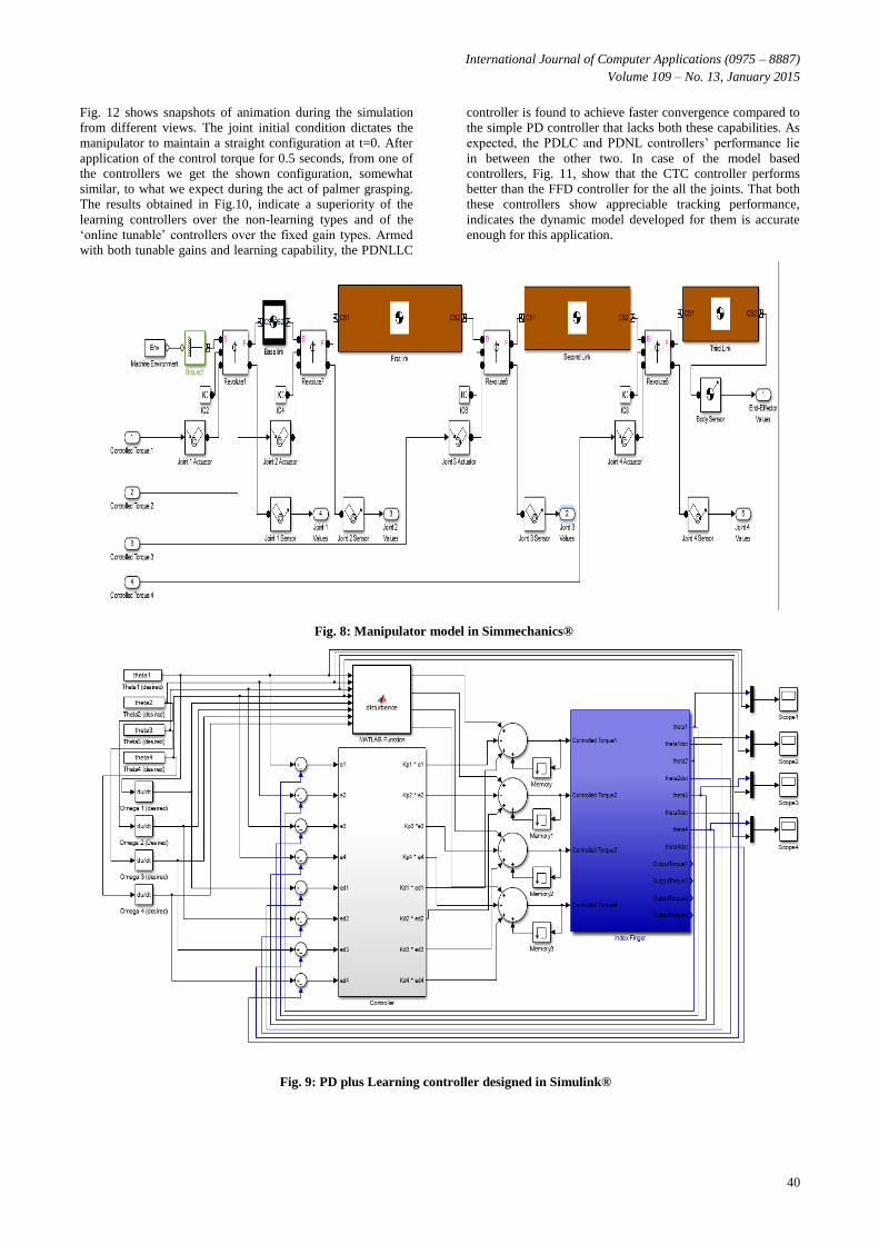
4. SIMULATION STUDY AND RESULTS As stated earlier, the designed control systems have been

tested on a model of only one „finger‟ having four revolute

joints. All other fingers can be designed in a similar manner.

Simulation has been carried out in MATLAB® using the

Control Systems Toolbox® and the Simmechanics® toolbox

[10, 13] of Simulink®. A virtual physical model of the plant

has been constructed using the inertia tensor of each link and

estimated masses and radii for the links. Every joint has been

actuated with the control torques for each controller. Joint

sensor blocks measure the angular positions and velocities for

providing the feedback. „MATLAB Function‟ blocks have

been used to set up the PD controllers and dynamic FFD

terms. All controllers have been tuned separately for best

performance, for which this is not a true comparison study,

though some expected results are obtained. The manipulator

as modeled in Simmechanics® is shown in Fig.8. The model

in Simmechanics® show the links, base link (in black) and

others (in brown), joint actuator, joint sensor, joint initial

condition blocks and other blocks to set environment effects

like ground/ reference and gravity. Link parameters are as per

Table 1.

Table 1. Link Parameters

Link Mass (kg) Length (m) Radius (m)

1 68.86e-6 0.002 0.002

2 38.73e-3 0.045 0.01

3 19.79e-3 0.023 0.01

4 17.21e-3 0.020 0.01

In accordance with 3D right handed co-ordinate system {x y

z}, gravity has been taken along the negative „y‟ direction.

Henceforth the various joints of the index finger, the MCP (2

DOF), the PIP and the DIP have been referred to as joints 1, 2,

3 and 4 respectively. While joint 1 revolves about the „y‟ axis,

all other joints revolve about the „z‟ axis.

The input signal i.e., the reference joint angle signal for each

joint is:

qd = 1+0.5sin(πt) (28)

The joint angular velocity and acceleration data wherever

required, are generated by differentiation of the above signal.

Fig.9 shows a screenshot of the complete Simulink model of

only one of the controllers, the PD plus Learning controller.

The controller was designed in Simulink® where the

subsystem (in blue) is the model shown in Fig.8 and the

controller that has been developed using „MATLAB function‟

blocks, is shown by another subsystem. The reference inputs

are introduced as time series variables. Here ‟Memory‟ blocks

feed in the value of the signal during the previous iteration.

We also introduce a FFD term for joint stiffness and damping

effects by the „Disturbance‟ subsystem. The „Theta‟ blocks

inject reference joint angle „qd‟ signals and they are

differentiated to obtain the „Omega‟ signals or reference joint

angular velocity „ q ‟ signals.

The PD and PDLC controllers have been set up with the

following gains:

Kp = diag. {800, 1350, 2800, 2800} and KD = diag. {15, 18,

10, 10}

The PDNL and PDNLLC controllers have been set up with

the following:

1maxp

K = 200; 2maxp

K = 150; 3maxp

K =200; 4maxp

K =200;

1minp

K =50; 2minp

K =100; 3min

pK =500; 4

minp

K =500;

10pK =1000; 20pK =1500;

30pK =3000; 40pK =3000. 1

maxd

K

=5; 2maxd

K =2; 3maxd

K =20; 4maxd

K =20;

1mind

K =2; 2mind

K =1; 3mind

K =5; 4mind

K =5;

10dK = 20; 20dK = 20;

30dK = 30; 40dK = 30;

a1 = a2 = a3 = a4 = 1.

For the FFD and the CTC controllers we have: Kp = diag.

{650, 900, 1100, 1100} and KD = diag. {10, 15, 8, 8}

The following figures show the (angular position) tracking

performance for the controllers while tracking the signal as

shown in equation(28). Fig.10, shows the performance of the

PD, PDNL, PDLC and PDNLLC controllers. The next four

figures, Fig.11, show the performance of the CTC and FFD

controllers. All angles are in radians.



40

Fig. 12 shows snapshots of animation during the simulation

from different views. The joint initial condition dictates the

manipulator to maintain a straight configuration at t=0. After

application of the control torque for 0.5 seconds, from one of

the controllers we get the shown configuration, somewhat

similar, to what we expect during the act of palmer grasping.

The results obtained in Fig.10, indicate a superiority of the

learning controllers over the non-learning types and of the

„online tunable‟ controllers over the fixed gain types. Armed

with both tunable gains and learning capability, the PDNLLC

controller is found to achieve faster convergence compared to

the simple PD controller that lacks both these capabilities. As

expected, the PDLC and PDNL controllers‟ performance lie

in between the other two. In case of the model based

controllers, Fig. 11, show that the CTC controller performs

better than the FFD controller for the all the joints. That both

these controllers show appreciable tracking performance,

indicates the dynamic model developed for them is accurate

enough for this application.

Fig. 8: Manipulator model in Simmechanics®

Fig. 9: PD plus Learning controller designed in Simulink®



41

(a)

(b)

(c)

(d)

Fig. 10. Tracking performance of Model free controllers: PD, PDNL, PDLC and PDNLLC controllers. (a) joint 1,

(b) joint 2, (c) joint 3, (d) joint 4.

(a)

(b)

(c)

(d)

Fig. 11. Tracking performance of Model based controllers: CTC and FFD controllers (a) joint1, (b) joint 2, (c) joint 3,

(d) joint 4.



42

(a)

(b)

Fig. 12: Animation snapshots (a) t=0 (b) t=0.5s

5. CONCLUSION The paper shows a preliminary study on position control

methods for a robotic manipulator that is being developed to

act as a human finger on a hand that can have multifarious

uses within the scope of Human Computer Interaction like

haptic rehabilitation applications. The aim of this manipulator

would be to mimic the human finger‟s complicated motion

during actions such as grasping an object. The controllers

developed are based on PD independent joint control and have

multiple PD loops in order to control a MIMO system as a set

of SISO systems. Improvements on the conventional PD

controller can be possible by introducing online gain tuning

and learning capabilities. The simulation tests carried out

confirm the superiority of these approaches over simple PD

control. Model based approaches, that take an inverse

dynamic plant model into consideration to reduce coupling of

parameters, have also been developed, that has fared better

than the model free approaches in the simulation tests

performed. However, the complicated inverse dynamic model

may be difficult to set up in software. Future work would

include developing a force control method based on PD and

model based strategies and subsequently a hybrid control

method (motion and force control) for the manipulator, prior

to manufacture and deployment of these strategies on

hardware. Modern control strategies like Model Predictive

Control are being studied to replace PD based controllers, if

viable.

6. ACKNOWLEDGMENTS This work was supported by the CSIR Supra Institutional

Project under 12th plan. The authors would like to gratefully

acknowledge the support and encouragement received from

Director, CSIR-CMERI, Durgapur.

7. REFERENCES [1] Mittal, R.K., Nagrath, I.J., 2003, Robotics and Control,

Tata Mc-Graw Hill Publishing Company Limited.

[2] Lewis, F.L., Dawson, D.M., Abdullah, C.T., 1993, Robot

Manipulator Control: Theory and Practice, Macmillan

Pub. Co.

[3] Craig, J.J., 1988, Adaptive Control of Mechanical

Manipulators, Addison-Wesley.

[4] Ouyang, P.R. and Zhang, W.J., 2004, “Comparison of

PD-based Controllers for robotic Manipulators”,

Proceedings of the ASME Design Engineering Technical

Conference.

[5] Ouyang, P.R, Zhang, W.J and M.M. Gupta, 2004,

“Adaptive nonlinear PD Learning Control of Robotic

Manipulators”, Proceedings of the ASME Design

Engineering Technical Conference.

[6] Paden, B. and Panja R., 1988, “Globally asymptotically

stable PD+ Controller for robot manipulators”,

International Journal of Control, Vol. 47, No. 6, pg.

1697-1712.

[7] An, C.H., Atkeson, C.G., Griffiths, J.D., Hollerbach,

J.M., 1989, “Experimental Evaluation of feedforward

and computed torque control”, IEEE Transactions on

Robotics and Automation, Vol. 5, Issue 3.

[8] Khosla P.K. and Kanade, T., 1988, “Experimental

Evaluation of Nonlinear Feedback and Feedforward

Control Schemes for Manipulators”, The International

Journal of Robotics Research, Vol. 7, No. 1, pg. 18-28.

[9] Santibanez, V. and Kelly, R., 2001, “PD control with

feedforward compensation for robot manipulators:

analysis and experimentation”, Robotica, Cambridge

University Press, Vol. 19, Issue 1, pg. 11-19.

[10] Dung, L.T., Kang, H. and Ro, Y., 2010, “Robot

Manipulator Modelling in Matlab-Simmechanics with

PD control and online Gravity Compensation”, IFOST

2010 Proceedings.

[11] De Luca, A., Siciliano, B. and Zollo, L., 2005, “PD

control with on-line gravity compensation for robots with

elastic joints: Theory and Experiments”, Automatica 41,

Elsevier, pg. 1809-1819.

[12] Middleton, R.H. and Goodwin, G.C., 1988, “Adaptive

computed torque control for rigid link manipulators”,

Systems and control Letters, Elsevier, Vol. 10, Issue 1,

pg. 9-16.

[13] MATLAB Simmechanics Documentation and User

Guide. (http://www.mathworks.in/help/physmod/sm/).

IJCATM : www.ijcaonline.org

http://www.mathworks.in/help/physmod/sm/

Motion Control Strategies based on PD Control for a...

Documents

Transcript of Motion Control Strategies based on PD Control for a...