Moon Ho Hwang DEVS++ verion 1.4 - DEVS++: C++...

Moon Ho HwangDEVS++ verion 1.4.2

ii

Copyright c©2005∼ 2009 Moon Ho Hwang ( http://moonho.hwang.googlepages.com/,

[email protected] ). All rights reserved.

You can cite this manual in the form of BibTex as follows.

@MANUAL{DEVSpp,

TITLE = "{DEVS++: C++ Open Source Library of DEVS Formalism}",

author = "Moon Ho Hwang",

address = "http://odevspp.sourceforge.net/",

edition = "v.1.4.2",

month = "April",

year = "2009",

}

Preface

Perfection is achieved, not when there is nothing more to add, but when thereis nothing left to take away.

- Antoine de Saint Exupery

DEVS++ is an open source library that is an implementation of discreteevent system specification (DEVS) formalism in C++ language. More than 30years ago, Dr. Zeigler introduced DEVS to the public through his first book[Zei76], and its second edition [ZPK00] became available in 2000 due to the helpof other two authors, Dr. Praehofer and Dr. Kim.

In 1994 when I was a Ph.D. student at the Korea Advanced Institute ofScience and Engineering (KAIST), I was taught the DEVS theory by Dr. Kimwho had been taught it by Dr. Zeigler. At that time, Dr. Kim used a C++library, called DEVSim++ c© [Kim94] in one of his courses. I became fascinatedwith it even at the first glance because I had been struggling with developinga simulator without any theory for a while. DEVSim++ was so neat and well-organized as is DEVS inherently.

After seeing the header files of DEVSim++, I developed several versionsof DEVS-based C++ kernels. One of them has been used in the VMS Lab.,directed by Dr. Byoung Kyu Choi, IE Dept. at KAIST, and some of them areused in commercial packages of Cubiteck Ltd. Co., Seoul, Korea.

I had a chance to meet Dr. Ziegler in the DEVS standardization session ofthe 2005 DEVS Symposium. At that time, Dr. Zeigler suggested that I open myC++ DEVS library (called DEVS++), and I accepted his suggestion. I releasedthe implementation as an open source project at http://odevspp.sourceforge.netin 2005. However, I were not able to finish writing its user manual over a coupleyears. Finally, the first version of the DEVS++ manual was released in May,2007 when DEVS++ has evolved up to version 1.4.1.

The main objective of this document is to introduce the DEVS++ library.Since it is a C++ implementation of DEVS formalism, we need to understandwhat DEVS is first. Chapter 1 provides a belief review of DEVS formalism byintroducing DEVS structures and their behaviors. Chapter 1 also gives sample

iv Preface

codes for a ping-pong game using DEVS++ so we can see what the DEVS++codes look like.

Chapter 2 explains the DEVS++ Library in terms of the object orientedprogramming paradigm of C++. We will see the class hierarchy and some ofthe virtual functions the user is supposed to override to make a concrete class.In addition, this section introduces a menu that DEVS++ provides when werun DEVS++ from a console.

Chapter 3 demonstrates several simple examples from atomic DEVS modelsto a coupled DEVS network. In these examples, we can check the knowledgelearned from the previous chapters.

Chapter 4 deals with one of major goals of simulation study, that is, howto measure some performance indices. To do this, the mathematical definitionsof throughput, cycle time, utilization and average queue length are addressedfirst, then their implementations in DEVS++ are introduced using practicalexamples. I hope the readers will have insight to modify these simple examplesfor their own purposes.

In addition to these main chapters, there are two appendixes. AppendixA explains how to build DEVS++ library from its source codes. Appendix Bsummaries the revision history and development plans of DEVS++.

Acknowledgements

I would thank Dr. Tag Gon Kim and Dr. Bernard. P. Zeigler for introducingme the world of DEVS.

Many thanks to

• Dr. Russ Mayers who read the entire document for version 1.4.1, correctedsome of my not so excellent English expressions, and suggested some inter-esting systems engineering ideas. Without his devoted help, this manualcould never have been completed.

• Shi Zhaoxiang who pointed out computation error of Example 4.5 so Iwere able to fix it when releasing the document of verion 1.4.2.

Special thanks are also due to my wife, Su Kyeon Cho, my mom Kyoung-AiKim, and my dad, Seung Hun Hwang who passed away in 2005 when the firstversion of DEVS++ was born.

Troy, MIMay 3, 2009

Moon Ho Hwang

Contents

Preface iii

1 DEVS Formalism and DEVS++ code 11.1 Atomic DEVS . . . . . . . . . . . . . . . . . . . . . . . . . . . . . 11.2 Coupled DEVS . . . . . . . . . . . . . . . . . . . . . . . . . . . . 41.3 Building Ping-Pong Game using DEVS++ . . . . . . . . . . . . . 6

2 Structure of DEVS++ 132.1 Event=PortValue . . . . . . . . . . . . . . . . . . . . . . . . . . . 14

2.1.1 Named . . . . . . . . . . . . . . . . . . . . . . . . . . . . . 142.1.2 Port, InputPort, and OutputPort . . . . . . . . . . . . . . 142.1.3 Value, bValue and tmValue . . . . . . . . . . . . . . . . . 152.1.4 PortValue . . . . . . . . . . . . . . . . . . . . . . . . . . . 16

2.2 DEVS . . . . . . . . . . . . . . . . . . . . . . . . . . . . . . . . . 162.2.1 Base DEVS: Devs . . . . . . . . . . . . . . . . . . . . . . 162.2.2 Atomic DEVS: Atomic . . . . . . . . . . . . . . . . . . . . 182.2.3 Coupled DEVS: Coupled . . . . . . . . . . . . . . . . . . 19

2.3 Scalable Real-Time Engine: SRTEngine . . . . . . . . . . . . . . 202.3.1 Constructor . . . . . . . . . . . . . . . . . . . . . . . . . . 202.3.2 Console Menu . . . . . . . . . . . . . . . . . . . . . . . . . 21

2.4 Random Variable . . . . . . . . . . . . . . . . . . . . . . . . . . . 242.5 Miscellaneous . . . . . . . . . . . . . . . . . . . . . . . . . . . . . 26

2.5.1 Time Span and Time . . . . . . . . . . . . . . . . . . . . 262.5.2 String Handling . . . . . . . . . . . . . . . . . . . . . . . . 26

3 Simple Examples 293.1 Atomic DEVS Examples . . . . . . . . . . . . . . . . . . . . . . . 29

3.1.1 Timer . . . . . . . . . . . . . . . . . . . . . . . . . . . . . 293.1.2 Vending Machine . . . . . . . . . . . . . . . . . . . . . . . 31

3.2 Coupled DEVS Examples . . . . . . . . . . . . . . . . . . . . . . 363.2.1 Monorail System . . . . . . . . . . . . . . . . . . . . . . . 36

vi CONTENTS

4 Performance Evaluation 434.1 Performance Measures . . . . . . . . . . . . . . . . . . . . . . . . 43

4.1.1 Throughput . . . . . . . . . . . . . . . . . . . . . . . . . . 434.1.2 Cycle Time . . . . . . . . . . . . . . . . . . . . . . . . . . 444.1.3 Utilization . . . . . . . . . . . . . . . . . . . . . . . . . . . 454.1.4 Average Queue Length . . . . . . . . . . . . . . . . . . . . 474.1.5 Sample Mean, Sample Variance, and Confidence Interval . 48

4.2 Practice in DEVS++ . . . . . . . . . . . . . . . . . . . . . . . . . 494.2.1 Throughput and System Time in DEVS++ . . . . . . . . 494.2.2 Utilization in DEVS++ . . . . . . . . . . . . . . . . . . . 534.2.3 Average Queue Length in DEVS++ . . . . . . . . . . . . 54

4.3 Client-Server System . . . . . . . . . . . . . . . . . . . . . . . . . 554.3.1 Server . . . . . . . . . . . . . . . . . . . . . . . . . . . . . 574.3.2 Buffer . . . . . . . . . . . . . . . . . . . . . . . . . . . . . 574.3.3 Performance Analysis . . . . . . . . . . . . . . . . . . . . 60

A Building DEVS++ 65A.1 Using Microsoft Visual Studio 2005TM . . . . . . . . . . . . . . . 65

A.1.1 When debugging through breakpoints in DEVS++ is failed 67

B History and Plan 69B.1 Revision History . . . . . . . . . . . . . . . . . . . . . . . . . . . 69

B.1.1 Version 1.4.2 . . . . . . . . . . . . . . . . . . . . . . . . . 69B.1.2 Version 1.4.1 . . . . . . . . . . . . . . . . . . . . . . . . . 69

B.2 Plan . . . . . . . . . . . . . . . . . . . . . . . . . . . . . . . . . . 71B.2.1 Short Term . . . . . . . . . . . . . . . . . . . . . . . . . . 71B.2.2 Mid Term . . . . . . . . . . . . . . . . . . . . . . . . . . . 71B.2.3 Long Term . . . . . . . . . . . . . . . . . . . . . . . . . . 71

List of Figures

1.1 Symmetric Structure of Atomic DEVS . . . . . . . . . . . . . . . 21.2 State Transition Diagram of Ping-Pong Player . . . . . . . . . . 41.3 DEVS Model of Ping-Pong Game . . . . . . . . . . . . . . . . . . 5

2.1 Classes in DEVS++ . . . . . . . . . . . . . . . . . . . . . . . . . 132.2 Relations of Times . . . . . . . . . . . . . . . . . . . . . . . . . . 17

3.1 SimplestTimer (a) State Transition Diagram (b) Event Segment (c) te Trajectory 303.2 State Transition Diagram of Vending Machine . . . . . . . . . . . 313.3 Monorail System . . . . . . . . . . . . . . . . . . . . . . . . . . . 363.4 Phase Transition Diagram of Station . . . . . . . . . . . . . . . . 37

4.1 A System having a Buffer and a Processor . . . . . . . . . . . . . 444.2 State Trajectory of a Processor . . . . . . . . . . . . . . . . . . . 454.3 A State Trajectory of Vending Machine . . . . . . . . . . . . . . 464.4 Trajectory of Queue . . . . . . . . . . . . . . . . . . . . . . . . . 474.5 IID random variants X1 . . . Xn from n simulation runs . . . . . . 484.6 Generator and Transducer in Ex ClientServer . . . . . . . . . . . 504.7 Configuration of Client Server System n = 3 . . . . . . . . . . . . 564.8 Server and Buffer . . . . . . . . . . . . . . . . . . . . . . . . . . . 564.9 Performance Indices . . . . . . . . . . . . . . . . . . . . . . . . . 62

A.1 Screen Capture of Visual Studio 2005TM when opening DEVSpp/DEVSpp.sln 66A.2 Change Debugger Type . . . . . . . . . . . . . . . . . . . . . . . 67

List of Tables

2.1 APIs related to Menu Items . . . . . . . . . . . . . . . . . . . . . 25

4.1 Performance Indices for each n = i of Servers . . . . . . . . . . . 61

Chapter 1

DEVS Formalism and

DEVS++ code

In DEVS formalism the time base denoted by T, is the non-negative real num-bers, i.e. T = [0,∞). Even though time can not reach the transfinite number,infinity (∞), sometimes it is useful to include ∞ in our consideration so we usethe extend set, denoted by T∞ = [0,∞].

This chapter introduces DEVS formalism in terms of the atomic DEVS todefine the dynamic behavior, and the coupled DEVS to build the hierarchicalnetwork structure.

1.1 Atomic DEVS

An atomic DEVS model is defined by a 7-tuple structure

A =< X,Y, S, s0, τ, δx, δy >

where

• X is a set of input events.

• Y is a set of output events.

• S is a set of partial states.

• s0 ∈ S is the initial partial state.

• τ : S → T∞ is the time advance function. This function is used todetermine the lifespan of a state.

2 DEVS Formalism and DEVS++ code

Figure 1.1: Symmetric Structure of Atomic DEVS

• δx : Q×X → S × {0, 1} is the external transition function where

Q = {(s, ts, te)|s ∈ S, ts ∈ T∞, te ∈ (T ∩ [0, ts])}

is the set of total states where ts and te are the lifespan of the state, s, andthe elapsed time since last reset of te, respectively. δx(s, ts, te) = (s′, b)defines how an input event, x, changes the state, s, as well as the lifespan,ts, and the elapsed time, te.

• δy : S → Y × S is the output and internal transition function that de-fines how a state generates an output event and, at the same time, howit changes the state internally. This function can be invoked when theelapsed time reaches the lifespan. 1

¥

Figure 1.1, also used as the cover illustration, shows the symmetric structureof DEVS in the sense that the input event set (X) and the external transitionfunction (δx) are on the input side; the output event set (Y ) and the outputand internal transition function (δy) are on the output side; and a set of states(S) and its time advance function (τ) are in the middle.

Definition 1.1 (Deterministic and Nondeterministic Functions) Let A

and B be two arbitrary sets. Then function f : A → B is called deterministicif give an a ∈ A, the values of callings f(a) at different times are identical.Otherwise, f is called non-deterministic. ¤

Definition 1.2 (Deterministic and Nondeterministic DEVSs) A DEVSmodel, M , is called deterministic if s0, τ, δx, and δy are deterministic. Other-wise, M is called non-deterministic. ¤

1In [ZPK00], δy is split into two functions: the output function λ : S → Y and the internal

transition function δint : S → S.

1.1 Atomic DEVS 3

Behavior of Atomic DEVS models

Suppose that A =< X, Y, S, s0, τ, δx, δy >is an atomic DEVS model. Thenbehavior of A is a sequence of total state transitions

(s, ts, te) → (s′, t′s, t′e)

where total states (s, ts, te) and (s′, t′s, t′e) ∈ Q are respectively defined at time

tl, tu ∈ T such that tl ≤ tu in the following three different cases.

1. Change by Time Passage If there is no event until time tu,

(a) (s′ = s) ∧ (t′s = ts), i.e, partial states and life spans are preserved,but

(b) the new elapsed time increases such that t′e = te + tu − tl.

We call move q to q′ total state change by time passage.

2. Change by an external transition When A receives an input eventx ∈ X,

(a) (s′, τ(s′), 0) if δx(q, x) = (s′, 1),

(b) (s, ts, te) if δx(q, x) = (s′, 0).

3. Change by an internal transition If there is no input event when tereaches at ts,2 then new state is defined as (s′, τ(s′), 0) if δy(s) = (y, s′).

For a formal definition of atomic DEVS behaviors, readers can refer to[DEV08a].

Example 1.1 (Ping-Pong Player) Figure 1.2 shows an atomic DEVS modelfor a ping-pong player. This model has an input event “?receive” and an outputevent “!send”. And it has two states: “Send” and “Wait”. Once the player getsinto “Send”, it will generates “!send” and backs to “Wait” after the sendingtime which is a random variant in the uniform probability distribution function(pdf) of [0.1, 1.2]. When staying at “Wait” and if it gets “?receive”, it changesinto “Send” again.

Formally we can rewrite this player as MPlayer =< X,Y, S, s0, τ, δx, δy >

where X={?receive}; Y ={!send};S={Send, Wait}; s0=Send; τ(Send)∈ [0.1,1.2], τ(Wait)=∞; δx(s, ts, te, x) = δx(Send,∞,[0,ts],?receive) =(Send,1),δx(s, ts, te, x) = δx(Send,[0.1, 1.2],[0,ts],?receive)=(Send,0);δy(s) = δy(Send)=(!send,Wait);

Notice that this player model is not deterministic because the lifespan valueof Send decided by τ(Send) is uniformly distributed in the interval of [0.1, 1.2].

¤2Recall that te ∈ T = [0,∞) and ts can be ∞. Thus when ts = ∞, it is impossible that

te = ts.


Figure 1.2: State Transition Diagram of Ping-Pong Player

1.2 Coupled DEVS

The coupled DEVS provides the hierarchical and modular structure necessaryto describe system networks. Formally, a coupled DEVS is defined by

N =< X, Y,D, {Mi}, EIC, ITC, EOC >

where

• X is a set of input events.

• Y is a set of output events.

• D is a set of names of sub-components

• {Mi} is a set of DEVS models where i ∈ D. Mi can be either an atomicDEVS model or a coupled DEVS model.

• EIC ⊆ X × ⋃i∈D

Xi is a set of external input couplings where Xi is the set

of input events of Mi.

• ITC ⊆ ⋃i∈D

Yi ×⋃

i∈D

Xi is a set of internal couplings where Yi is the set of

output events of Mi.

• EOC ⊆ ⋃i∈D

Yi × Y is a set of external output couplings. ¥

Practically, we can see an event as a pair of (port, value) and the couplingas a pair of (portsource, portdestination) [Zei90, ZPK00]. The basic assump-tion of the port coupling is that the value of portsource is casted to that ofportdestination. We can find that the realistic example of the port coupling inthe VHDL language [Ska96] and the language of programmable logic controller(PLC) [Lew98]. DEVS++ implements the (port,value) view for events (we willsee it in Section 2.1.4). However, it does not mean that the event should be apair of a port and a value.

1.2 Coupled DEVS 5

Figure 1.3: DEVS Model of Ping-Pong Game

Behavior of Coupled DEVS models

The coupled DEVS’s behavior is described verbally as follows.

1. Change by Time Passage If there are no events in time duration tl totu(tl ≤ tu), all sub-components’ total states are changed by time passageof dt = tu − tl.

2. Change by an external transition When N receives an input event, thecoupled DEVS transmits the input event to the sub-components throughthe set of external input couplings.

3. Change by an internal transition When a sub-component producesits output event when the internal transition occurs, the coupled DEVStransmits the output event to the other sub-components through the setof internal couplings. The coupled DEVS also produces an output eventof N through the set of external output couplings.

Theoretically speaking, DEVS is closed under the coupling which means thatthe behavior of any coupled DEVS model can be explained by an atomic DEVSmodel.[ZPK00]. For a formal definition of coupled DEVS behaviors, readers canrefer to [DEV08b].

Example 1.2 (Ping-Pong Game) Consider a ping-pong game with two play-ers that each represented by the Player model introduced in Example 1.1 exceptthe initial state.

This block diagram can be modeled by a coupled DEVS such as NPPGame =<

X, Y,D, {Mi}, EIC, ITC,EOC > where X = {}; Y = {};D={A,B}; {Mi} ={Playeri}where Playeri is the atomic DEVS introduced in Example 1.1 with initialstates Send for i=A, Wait for i=B, respectively; EIC={ }, ITC={ (A.!send,B.?receive), (B.!send, A.?receive)}, EOC = { }. ¤


1.3 Building Ping-Pong Game using DEVS++

This section shows how DEVS++ codes look like using the ping-pong game intro-duced in Example 1.2. All source codes below are available in DEVSpp/Examples/Ex_PinPong

folder. If you want to build and run this example by yourself, Appendix A willbe helpful for you.

#include "Atomic.h" //--- (1)

#include "Coupled.h"

#include "SRTEngine.h"

#include "RNG.h"

#include <iostream>

#include <math.h>

using namespace std;

using namespace DEVSpp; //--- (2)

const string WAIT = "Wait";

const string SEND = "Send";

//---- definition of atomic DEVS for Player --- (3)

class Player: public Atomic {

public:

OutputPort* send; //-- associated ports --- (4)

InputPort* receive;

protected: //-- associated internal state variables ----(5)

string m_phase;

bool m_width_ball;

public:

Player(const string& name="", bool with_ball=false): Atomic(name),

m_phase(WAIT), m_width_ball(with_ball)

{

send = AddOP("send"); //--- add ports --- (6)

receive = AddIP("receive");

}

//---- four characteristic functions ------- (7)

/*virtual*/ void init()

{

if(m_width_ball)

m_phase = SEND;

else

m_phase = WAIT;

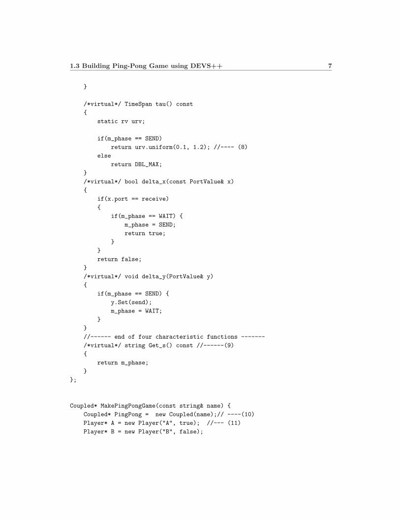
1.3 Building Ping-Pong Game using DEVS++ 7

}

/*virtual*/ TimeSpan tau() const

{

static rv urv;

if(m_phase == SEND)

return urv.uniform(0.1, 1.2); //---- (8)

else

return DBL_MAX;

}

/*virtual*/ bool delta_x(const PortValue& x)

{

if(x.port == receive)

{

if(m_phase == WAIT) {

m_phase = SEND;

return true;

}

}

return false;

}

/*virtual*/ void delta_y(PortValue& y)

{

if(m_phase == SEND) {

y.Set(send);

m_phase = WAIT;

}

}

//------ end of four characteristic functions -------

/*virtual*/ string Get_s() const //------(9)

{

return m_phase;

}

};

Coupled* MakePingPongGame(const string& name) {

Coupled* PingPong = new Coupled(name);// ----(10)

Player* A = new Player("A", true); //--- (11)

Player* B = new Player("B", false);


A->CollectStatistics(true); //-- (12)

B->CollectStatistics(true);

PingPong->AddModel(A); //-- (13)

PingPong->AddModel(B);

//-- Internal Coupling -------- (14)

PingPong->AddCP(A->send, B->receive);

PingPong->AddCP(B->send, A->receive);

PingPong->PrintCouplings(); //---- (15)

return PingPong;

}

void main(void) {

Coupled* PingPong = MakePingPongGame("PingPong");

SRTEngine simEngine(*PingPong);//-- (16)

simEngine.RunConsoleMenu(); //-- (17)

delete PingPong;

}

Above example codes contain comments in the forms of“//--- (#)”. Each “(#)” has the following explanation.

(1) Include Files

First of all, we should include the associated header files. In this example, wedefine the class Player derived from the class Atomic (Atomic.h); we createa ping-pong game as an instance of the class Coupled (Coupled.h); we willsimulate the ping-pong game using a scalable simulation engine: SRTEngine

(SRTEngine.h); and the time advance of the state Send is a random variable ofthe uniform pdf (RNG.h).

(2) Using Name Space

For convenience, we use the name space “DEVSpp” as well as “std”. Withoutthis, we should add a scope operator like DEVSpp:: or std:: in front of allclasses and global APIs that are defined in DEVSpp and std.

(3) Player derived from Atomic

In this example, Player is a concrete class derived from Atomic which is anabstract class. We will see the class Atomic in Section 2.2.2.


(4) Interfacing Ports

The port pointers are useful to identify the added ports. Without these pointers,we would have to search for each pointer by its name, and that can be a burden.For more information of the class Port, the reader can refer to Section 2.1.2

(5) State Variables

The derived and concrete class of atomic DEVS will have its state variables todescribe its dynamic situations. In DEVS++, we use member data of C++ forthe state variables.

(6) Adding Interfacing Ports

The interfacing port pointers mentioned in (5) are assigned by calling either theAddIP or the AddOP function in which memory allocations and parent assign-ments are performed. A set of port related functions defined at Atomic can bereferred to Section 2.2.2.

(7) Defining Four Characteristic Functions

The characteristic functions such as τ, δx, δy plus init() are pure virtual, andso we should override them when defining a concrete class of Atomic. Thesecharacteristic functions describe the behavior of the state transition diagram ofFigure 1.3.

(8) Random Number

The lifespan of Send is a random variable with uniform pdf of [0.1,1.2], whereelements of the domain denote time-units. To generate the random number, therandom variable class rv is used as a static local variable for the output of thefunction tau(). The pdfs available in DEVS++ are addressed in Section 2.4.

(9) Displaying the current state

To show the current state, we will override the Get_s() function which is sup-posed to return the current state in a string.

(10) Making the Ping-Pong Game

We make an instance of coupled DEVS for the ping-pong game.

(11) Creating Two Players

The ping-pong game has two sub-components that are instances of Player hav-ing different initial states.


(12) Collecting Statistics

If we want to collect statistics about the two players, we turn the flag on bycalling CollectStatistics(true). Chapter 4 will introduce performance mea-sures and how we can collect statistics in detail.

(13) Adding Sub-components

We add two players A and B by calling the function AddModel of the classCoupled.

(14) Adding Couplings

We add couplings between players A and B calling the function AddCP of theclass Coupled .

(15) Print Couplings

Even though it is not necessary, we can call the function PrintCouplings() ofCoupled to check the coupling status. The couplings of the ping-pong game aredisplayed as follows.

Inside of PingPong

-- External Input Coupling (EIC) --

------ # of EICs: 0-----

-- Internal Coupling (ITC) --

A.send --> B.receive

B.send --> A.receive

------ # of ITCs: 2-----

-- External Output Coupling (EOC) --

------ # of EOCs: 0-----

(16) Making a simulation engine

Instancing a scalable simulation engine SRTEngine can be done by calling itsconstructor that needs the model supposed to be simulated. In this examplethe model is the coupled model of the ping-pong game.

(17) Running the console menu

We can use the console menu of SRTEngine by calling RunConsoleMenu(). Afterthat, we will see the following screen on the selected console.


DEVS++: C++ Open Source of DEVS Implementation, (C) 2005~2009,

http://odevspp.sourceforge.net

The current date is 04/09/09

The current time is 11:42:26

scale, step, run, mrun, [p]ause, pause_at, [c]ontinue, reset,

rerun, [i]nject, dtmode, animode, print, cls, log, [e]xit

>

The first part shows the header of DEVS++ and current data and time.The second part shows the available command set. Even we don’t have clearidea of each command, let’s try“ run” and then “exit”.

The detailed information of each command will be provided in Section 2.3.

Chapter 2

Structure of DEVS++

DEVS++ is an C++ open source of DEVS formalism. Thus, there are twofeatures: one comes from C++ language, the other from the formalism. Figure2.1 shows the hierarchy relation among classes used in DEVS++.

As we reviewed in Chapter 1, two DEVS models called atomic DEVS andcoupled DEVS have common features such as input and output event interfacesas well as time features such as current time, elapsed time, schedule time andso on. In DEVS++, these common features have been captured by a baseclass, called Devs from which the class Atomic (for atomic DEVS) and the classCoupled (for coupled DEVS) are derived.

In DEVS++, an event is a pair of (port, value) where port can be an instanceof either InputPort class or OutputPort class, while value is an instance ofa derived class of Value class such as bValue and tmValue. SRTEngine is ascalable real-time engine which runs a DEVS instance inside. rv is a class for arandom variable.

In Figure 2.1, a gray box indicates a concrete class which can be created asan instance, while a white box is an abstract class which can not be created as

Figure 2.1: Classes in DEVS++

14 Structure of DEVS++

an instance.We will first go through the PortValue class and its related classes in Section

2.1. Next, Devs class and its derived two classes: Atomic and Coupled will beinvestigated in Section 2.2, Section 2.3 will introduce a simulation engine class,called SRTEngine. And finally, We will see the random number generator rv inSection 2.4.

2.1 Event=PortValue

An event will be modeled by an instance of PortValue class which is a pair ofPort and Value. We will first see the top-most base class, called “Named”. Thenwe will look at Port-related classes and Value-related classes. And finally, thePortValue class will be seen in the last part of this section.

2.1.1 Named

Named is defined in a header file Named.h as a concrete class. The class providesits constructor whose argument is a string, and has a public Name field as astring.

class Named {

public:

Named(const string& name):Name(name){}

string Name;

};

2.1.2 Port, InputPort, and OutputPort

The Port.h file defines three classes Port, InputPort and OutputPort as fol-lows.

class Port: public Named {

public:

Devs* Parent;

vector<Port*> ToP; // Successor

vector<Port*> FromP; // Predecessor

...

};

class InputPort: public Port {

...

};

2.1 Event=PortValue 15

class OutputPort: public Port {

...

};

Port is an abstract class derived from Named. It has a parent pointer whose typeis Devs pointer and which is automatically assigned when we call the AddIP()

and AddOP() functions of Devs. Port has “vector<Port*> ToP” as a set ofsuccessors as well as “vector<Port*> FromP” as a set of predecessors whichare changed when we call AddCP() and RemoveCP() of Coupled.

InputPort and OutputPort are concrete and derived classes from Port.

2.1.3 Value, bValue and tmValue

In Value.h, there are three classes: Value, bValue and tmValue. Value is thebase abstract class for the other two classes. Value has two virtual functions:Clone() makes a copy, STR() returns a string of a derived class’s status.

class Value {

protected:

Value(){}

public:

virtual Value* Clone() const {return NULL;}

virtual string STR() const {return string(); }

};

bValue is a concrete class derived from Value. bValue is a template class,and it has a field v whose type is the template augment V. Thus we can de-fine bValue<bool>, bValue<char>, bValue<int>, bValue<double> whose valuetypes are bool, char, int, and double, respectively.

template<class V>

class bValue: public Value {

public:

V v; //-- public value field

...

};

tmValue is a concrete class derived from Value. This class has a map froma string to a double-precision floating number that can be used to identify anevent as a string and to specify its occurrence time.

class tmValue: public Value {

public:

map<string, double> TimeMap;


...

};

You can see how to use this tmValue in Section 4.2.1 and 4.3.

2.1.4 PortValue

As mentioned before, an event in DEVS++ is modeled by a pair of associatedclasses: Port and Value by using the PortValue class.

class PortValue {

public:

Port* port; //-- either an output port or an input port

Value* value;//-- typecast it to a concrete derived class!

PortValue(const Port* p=NULL, Value* v=NULL);

...

};

2.2 DEVS

As introduced in Chapter 1, DEVS has two basic structures: atomic DEVSand coupled DEVS. In DEVS++, these two structures are implemented as theclasses Atomic and Coupled, respectively, and are derived from the base classDevs. Thus Devs has the common member data and functions of both Atomic

and Coupled.

2.2.1 Base DEVS: Devs

Devs defined in Devs.h is an abstract class derived from Named.1 And it hasthe parent pointer assigned by AddModel() of Coupled as we will see in Section2.2.3.

class DEVSpp_EXP Devs: public Named {

public:

Coupled* Parent; // parent pointer

...

There are adding, getting, removing, and printing functions for the inputports denoted as AddIP, GetIP, RemoveIP, and PrintAllIPs. Similarly, AddOP,GetOP, RemoveOP, and PrintAllOPs are available functions for the output ports.

1The macro DEVSpp EXP can be compiled several different ways according to the set of

preprocessor. For compiling dynamic linking library, we should add DLL in the preprocessor

definitions. For more information, the reader can refer to Chapter A.

2.2 DEVS 17

Figure 2.2: Relations of Times

//-- Input Port related functions --

InputPort* AddIP(const string& ipn);

InputPort* GetIP(const string& ipn) const;

InputPort* RemoveIP(const string& ipn);

void PrintAllIPs() const;

//-- Output Port related functions --

OutputPort* AddOP(const string& opn);

OutputPort* GetOP(const string& opn) const;

OutputPort* RemoveOP(const string& opn);

void PrintAllOPs() const;

Implementations of Times

Recall that the behavior of DEVS needs times notions, lifespan ts and elapsedtime te (see section 2.2.2). To capture these two times, DEVS++ implementstwo other time notions: last event time tl and next event time tn instead. If wehave a current time, tc, relationships among them are

ts = tn − tl,

te = tc − tl

andtr = ts − te = tn − tc

where tr is remaining time to tn. Figure 2.2 illustrates the relationships amongthese times.

The user doesn’t have to set the values of times during simulation since thatwill be done by DEVS++. However, if users need to access the values of them,there are following APIs defined at Devs class :


Time TimeLast() const;

Time TimeNext() const ;

Time TimeLifespan() const ;

static Time TimeCurrent() ;

Time TimeElapsed() const ;

Time TimeRemaining() const ;

Notice that TimeCurrent() is a static function which means that all DEVS in-stances will have the same value of TimeCurrent(), while they can have differentvalues for TimeLast(), TimeNext(), etc.

2.2.2 Atomic DEVS: Atomic

The atomic DEVS is implemented as Atomic in the files of Atomic.h andAtomic.cpp. Atomic is an abstract class that is derived from the abstract baseclass Devs.

class DEVSpp_EXP Atomic: public Devs {

protected:

Atomic(const string& name): Devs(name), m_cs(false) {}

...

Characteristic Functions

There are four public characteristic functions that are pure virtual. Thus theuser must override them to define a concrete class from Atomic.

The function init() is used when the model needs to be reset, such as inthe case of an initialization for a simulation run.

virtual void init() = 0;

The function tau() returns the lifespan of the current state.

virtual TimeSpan tau() const = 0;

The function delta_x(const_PortValue& x) defines the input state transi-tion caused by an input event x. The return value true indicates that the nextschedule needs to be updated by calling tau(). Contrarily, the return valuefalse indicates that the time for the next schedule needs to be preserved.

virtual bool delta_x(const PortValue& x) = 0;

The function delta_y(PortValue& y) defines the output transition by gen-erating an output event y. Recall that the schedule will be updated right afterthis occurs, based upon the value of tau().

virtual void delta_y(PortValue& y) = 0;

2.2 DEVS 19

Displaying State as a string

There is an other public virtual(but not pure) function Get_s(), that will returnthe current status in a string for display purposes.

virtual string Get_s() const { return string();}

Collecting Performance Functions

If we want to trace the performance of an atomic DEVS model, we need to set theflag on by using CollectStatistics(true). We can also get the flag’s status bycalling CollectStatisticsFlag(). The virtual function Get_Statistics_s()

will return a string which represents the status in terms of collecting statis-tics. Also, the user can override the GetPerformance() function to collect theperformance index.

void CollectStatistics(bool flag = true) { m_cs = flag; }

bool CollectStatisticsFlag() const { return m_cs; }

virtual string Get_Statistics_s() const { return Get_s(); }

virtual map<string, double> GetPerformance() const;

We will see the theoretical background of performance indices and how wecollect them using DEVS++ in Chapter 4.

2.2.3 Coupled DEVS: Coupled

The coupled DEVS is implemented as the class Coupled derived from the classDevs. Coupled class is concrete and it has a constructor. It also has a destructorin which all sub-components are deleted.

class DEVSpp_EXP Coupled: public Devs {

public:

Coupled(const string& name=""): Devs(name) {}

virtual ~Coupled();

Sub-components Related

There are three main functions associated with modeling of sub-components asfollows.

void AddModel(Devs* md);

Devs* GetModel(const string& name) const;

void RemoveModel(Devs* md);


Couplings Related

Related to couplings, there are three constructing functions, one each for theexternal input couplings (EICs), the internal couplings (ITCs), and the externaloutput couplings (EOCs).

void AddCP(InputPort* spt, InputPort* dpt); // EIC

void AddCP(OutputPort* spt, InputPort* dpt); // ITC

void AddCP(OutputPort* spt, OutputPort* dpt);// EOC

In addition, we can print out the coupling information by calling PrintEICs(),PrintITCs(), PrintEOCs(), and PrintCouplings() for printing EICs, ITCs,and EOCs, and all of them, respectively.

void PrintEICs() const;

void PrintITCs() const;

void PrintEOCs() const;

void PrintCouplings() const;

The corresponding removing functions are as follows.

void RemoveCP(InputPort* spt, InputPort* dpt); // EIC

void RemoveCP(OutputPort* spt, InputPort* dpt); // ITC

void RemoveCP(OutputPort* spt, OutputPort* dpt);// EOC

2.3 Scalable Real-Time Engine: SRTEngine

DEVS++ provides a simulation engine class, called SRTEngine which is a con-crete class. When we make an instance of SRTEngine, its constructor createsan independent simulation thread from the main thread.

2.3.1 Constructor

SRTEngine(Devs& modl, Time ending_t = DBL_MAX, CallBack cbf=NULL);

The constructor needs three arguments: the first argument is the Devs modelto be simulated, the second is the simulation terminating time, the last is acallback function that is used to inject a user-input into the simulation model.

Callback function’s type is defined as

PortValue (*CallBack)(Devs& md).

It returns a PortValue which can be a pair of an input port and a value. Theassociated input port should belong to Devs md. The following example showsthat InjectMsg returns a PortValue whose port is vm’s ip input port.

2.3 Scalable Real-Time Engine: SRTEngine 21

PortValue InjectMsg(Devs& md) {

VM& vm = (VM&) md;

return PortValue(vm.ip);

}

We can pass the function pointer of a callback function to an instance ofSRTEngine as follows.

SRTEngine simEngine(vm, 10000, InjectMsg);

2.3.2 Console Menu

If we call the RunConsoleMenu() function of SRTEngine, it provides a consolemenu as follows.

scale, step, run, mrun, [p]ause, pause_at, [c]ontinue, reset,

rerun, [i]nject, dtmode, animode, print, cls, log, [e]xit

>

Let’s take a look at each menu item.

scale f

scale controls the speed of time flow by the scale factor f

• 0.1 for 10 times slower than real time

• 1 as fast as real time;

• 10 for 10 times faster than real time;

• 0 or greater than 1000,000 for as fast as possible;

step

step executes a simulation run until one internal transition is fired. After thatit pauses the run automatically unless the user inputs commands such as step,continue, run, mrun. This command can be useful when we try a step-by-steprun to see the model behavior.

run

run executes a simulation run which continues until it reaches the simulationending time, which is set by the second argument of the SRTEngine constructoror by the command pause_at et.


mrun n

mrun executes n simulation runs. Each simulation run stops when it reaches thesimulation ending time. When trying mrun n, where 2≤ n ≤ 20, SRTEinginecalculates the 95% confidence interval of the average values of each statisticalitems.

[p]ause

pause or p pauses a simulation run immediately.

pause at et

pause_at sets the simulation ending time as et.

[c]ontinue

continue or c resumes a simulation run which has been paused. It continuesthe previous simulation mode that had been determined by step, run, or mrun.

reset

reset initializes the associated simulation model.

rerun

rerun combines reset and run.

[i]nject

inject or i injects an user-input event into the simulation model. This com-mand invokes the callback function whose type is PortValue callback(Devs& md).This is the third argument of the SRTEngine constructor.

dtmode

dtmode sets the print mode of discrete transition, both for in the console and inthe log file (whose file name is devspp_log.txt). The choice can be one of thefollowing options:

• none displays no discrete state transition.

• rel displays relative mode in which lifespan and elapsed time are dis-played.

• abs displays absolute mode in which last event time and n ext event timeare displayed.

2.3 Scalable Real-Time Engine: SRTEngine 23

• nc no change.

animode

animode sets the animation interval. The choice can be either one of the fol-lowing options.

• none displays no animation state transition.

• ani is the number of animation interval > 1.0E-2.

• nc no change.

print

print displays information according to the following option.

• q prints the total state of the model.

• cpl prints the couplings information if the model is a coupled DEVS.

• s prints all settings. The following screen shot is made by print s.

scale factor: 1

run-through mode

current time: 0

simulation ending time: 1.79769e+308

current dt_mode: absolute

current animation mode: on and interval= 0.25

current log setting: on, p00

• p prints the performance indices at the current time.

cls

cls clears the screen.

log

log sets the logging option which generates the log file devspp_log.txt. Afterthe log command, DEVS++ shows the current log settings and waits for theuser input as follows.

current log setting: on, p00

options: {on,off}, {+,-}{pqt} nc >

The user options are on or off or {+,-}{pqt} or nc. Their meanings are:


• {on, off} is the main log options. Use on for turning log on or off forturning log off. If the mode is on, three independent options are selectable.

– p is for logging performance indices at the end of a simulation run.

– q is for logging the total state of the model at the end of a simulationrun.

– t is for logging every single discrete event transition.

If all of three are on, it is shown as pqt. If p is on, q and t are off, thedisplay is shown as p00, etc.

• {+,-}{pqt} can be interpreted that + stands for setting the followingoptions on, while - stands for turning the following options off. Forexample +qt means to set q and t on, while -p means to set p off.

• nc no change.

[e]xit

exit or e exits the console menu.Table 2.1 summarizes API functions of SRTEngine related to menu items

that we have introduced so far.

2.4 Random Variable

DEVS++ modified the random number generator that was provided with theADEVS engine [Nut00] in 2004. rv class defined in RNG.h is a random vari-able whose default constructor rv() sets its seed number as the current time.There are four probability density functions that can be used to select a randomnumber: uniform, triangular, exponential, normal.

1. uniform(a,b) returns a random number having a uniform PDF over theclosed interval [a,b].

2. triangular(a,b,c) returns a random number having a triangular PDFover the closed interval [a,b] with mode c, where c in [a,b].

3. exp(m) returns a random number having an exponential PDF with meanm.

4. normal(m,s) returns a random number having a normal PDF with meanm and standard deviation s.

2.4 Random Variable 25

Table 2.1: APIs related to Menu Items

Menu Item SRTEngine’s APIs

scale double GetTimeScale() const;

void SetTimeScale(double ts);

step void Step();

run void MultiRun(1);

mrun n void MultiRun(unsigned n);

pause void Pause();

pause_at Time GetEndingTime() const;

void SetEndingTime(Time et);

continue void Continue();

reset void Reset();

rerun void Rerun();

inject void Inject(PortValue x);

dtmode void Set_dtmode(PrintStateMode flag);

void Get_dtmode(PrintStateMode& flag) const;

whereenum PrintStateMode {P_NONE, P_relative, P_absolute};

animode void SetAnimationFlag(bool flag);

bool GetAnimationFlag() const;

void SetAnimationInterval(TimeSpan ai);

TimeSpan GetAnimationInterval() const;

print void PrintTotalState() const;

void PrintCouplings() const;

void PrintSettings() const;

void PrintPerformanceOfaRun() const;

log static void SetLogOn(bool flag=true);

static void SetLogPerformance(bool flag=true);

static void SetLogTotalState(bool flag=true);

static void SetLogTransition(bool flag=true);

static bool GetLogOn();

static bool GetLogPerformance();

static bool GetLogTotalState();

static bool GetLogTransition();


2.5 Miscellaneous

2.5.1 Time Span and Time

Sometimes, we are confused with two concepts: time span and time. A timespan means the time duration between a starting time and an ending timein which the starting time and the ending time are specific values within thetime horizon. In general, the time horizon consists of all the non-negative realnumbers. But a time value is for a specific value within the time horizon.

In DEVS++, both TimeSpan and Time are defined as double in Devs.h.

typedef double TimeSpan ;

typedef double Time;

When we want to check if a pair a and b are the same in terms of a tolerancetol, we can use the following function defined in Devs.h.

bool DEVSpp::IsEqual(double a, double b, double tol=1E-3);

Since both types of a and b are double, we can be for checking for Time andTimeSpan, respectively.

We can also check if a given real number is equal to infinity by the followingfunction

bool DEVSpp::IsInfinity(double a, double tol);

in which it calls IsEqual(a, DBL_MAX, tol).

2.5.2 String Handling

String handling functions inside of the DEVSpp name space are available inStrUtil.h and StrUtil.cpp.

string STR(int v);// return int v as a string

string STR(conststring& s,int v);//s+::STR(v);

string STR(unsigned v); // return int v as a string

string STR(const string& s, unsigned v);//s+::STR(v);

string STR(double v);// return int v as a string

string STR(const string& s, double v);//s+::STR(v);

//-- split string s using delimiter c by n times if possible

vector<string> Split(const string& s, char c);

//-- return the merged string with s from f to t with delimiter c

string Merge(const vector<string>& s, unsigned f, char c);

2.5 Miscellaneous 27

//-- return string(pt->Parent->Name+"."+pt->Name);

string NameWithParent(DEVSpp::Port* pt);

//-- hierarchical name of child from the view of under.

//-- if under=NULL, the hierarchical name starts from the root model

string HierName(const Devs* child, const Coupled* under=NULL);

Chapter 3

Simple Examples

In this chapter, we will see DEVS++ examples of atomic DEVS as well ascoupled DEVS.

3.1 Atomic DEVS Examples

3.1.1 Timer

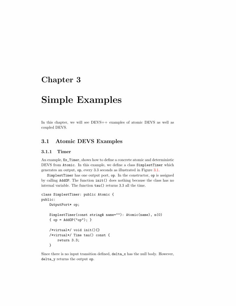
An example, Ex_Timer, shows how to define a concrete atomic and deterministicDEVS from Atomic. In this example, we define a class SimplestTimer whichgenerates an output, op, every 3.3 seconds as illustrated in Figure 3.1.

SimplestTimer has one output port, op. In the constructor, op is assignedby calling AddOP. The function init() does nothing because the class has nointernal variable. The function tau() returns 3.3 all the time.

class SimplestTimer: public Atomic {

public:

OutputPort* op;

SimplestTimer(const string& name=""): Atomic(name), n(0)

{ op = AddOP("op"); }

/*virtual*/ void init(){}

/*virtual*/ Time tau() const {

return 3.3;

}

Since there is no input transition defined, delta_x has the null body. However,delta_y returns the output op.

30 Simple Examples

Figure 3.1: SimplestTimer (a) State Transition Diagram (b) Event Segment (c)te Trajectory

/*virtual*/ bool delta_x(const PortValue& x) {return false;}


{

y.Set(op);

}

The display function Get_s() returns the current status, which is constantlyWorking.

/*virtual*/ string Get_s() const {

return string("Working");

}

};

If you try step, you can see the animation is increasing the elapsed time.The following display shows the state at time 2.188 where the schedule timet_s=3.3 and the elapsed time t_e=2.188.

(STimer:Working, t_s=3.300, t_e=2.188) at 2.188

The simulation run will stop at 3.3 because its run mode is step-by-step whenusing step. At that time, it will display the discrete state transition as follows.

(STimer:Working, t_s=3.300, t_e=3.300)

--({!STimer.op},t_c=3.3)-->

(STimer:Working, t_s=3.300, t_e=0.000)

The first state is the source of state transition. An arc shows a triggering eventwhich is the output op of STimer at the current time=3.3. The second state isthe destination of the state transition in which the lifespan is also 3.3 but theelapsed time has been reset to zero.

3.1 Atomic DEVS Examples 31

Figure 3.2: State Transition Diagram of Vending Machine

Exercise 3.1 Consider the example Ex_Timer.

a. Let’s change the display mode from rel to abs by applying the commanddtmode. Then preset the simulation ending time to “5” by pause_at 5.Now run until the simulation stops. When it stops at t_c=5, print thetotal state using pinrt with option q. What are the values of t_s andt_e, respectively? Guess the remaining time that t_e becomes t_s (ort_c becomes t_n) at this moment.

b. Add one more state variable int n in SimplestTimer class. n should beset = zero in init(), and it should increase by one in delta_y(). Get_s()shows n in the C print format of "Working, n=%d".

3.1.2 Vending Machine

Consider a simple vending machine (VM) from which we can get Pepsi and Coke.Figure 3.2 illustrates the state transition diagram of VM we are considering.

There are three input events such as ?dollar for “input a dollar”, ?pepsi_btnfor “push the Pepsi button”, ?coke_btn for “push the Coke button”. Similarly,we can model three output events such as !dollar for “a dollar out (becauseof timeout of menu selection)”, !pepsi for “Pepsi out” and !coke for “Cokeout’. 1 The state of VM can be either Idle for “Idle”, Wait for “Wait”(that iswaiting for selection of Pesi or Coke), O_Pepsi for “output Pepsi” and O_Coke

for “output Coke”. And their life times are: 15 time units for Wait, 2 timeunites for both O_Pepsi and O_Coke, ∞ for Idle which is denoted by inf inFigure 3.2. 2

1We use symbol ? and ! for indicating an input event and an output event, respectively.2we call a state s passive if τ(s) = ∞ or active otherwise (0 ≤ τ(s) < ∞). In Figure 3.2,

the state Idle is passive, the rest states are active.

32 Simple Examples

At the beginning (t=0), VM is at Idle. If we put ?dollar in, it changes thestate into Wait simultaneously updating ts = 15 and te = 0 for the state. Whilein the state, if VM receives ?pepsi_btn (resp. ?coke_btn), it enters into thestate O_Pepsi (resp. O_Coke) and simultaneously updates ts = 2 and te = 0.While in the state O_Pepsi or O_Coke, VM ignores any input and preserves thestate. Similarly, while in the state Wait, VM ignores ?dollar input.

After staying at Wait for 15 time unites, VM returns to Idle state and outputsthe dollar if we don’t select Pepi or Coke within the 15 time units. However, ifwe had selected one of them, VM changes its state into O_Pepsi (resp. O_Coke).Then after 2 time unites, VM outputs !pepsi (resp. !coke) and returns to Idle.

The example of Ex_VendingMachine shows an atomic DEVS model of VM.First of all, there are some constant strings we use for describing states asfollows.

const string IDLE="Idle";

const string WAIT="Wait";

const string O_PEPSI="O_Pepsi";

const string O_COKE="O_Coke";

The class VM has three input port pointers idollar, pepsi_btn and coke_btn;three output port pointers odollar, pepsi, coke, all assigned by returning val-ues of the AddIP and AddOP functions in the constructor.

class VM: public Atomic {

public:

InputPort * idollar, *pepsi_btn, *coke_btn;

OutputPort * odollar, *pepsi, *coke;

VM(const string& name=""): Atomic(name)

{

idollar = AddIP("dollar");

pepsi_btn = AddIP("pepsi_btn");

coke_btn = AddIP("coke_btn");

odollar = AddOP("dollar");

pepsi = AddOP("pepsi");

coke = AddOP("coke");

init();

}

VM’s initial state is set to IDLE in init(). The lifespan of each state isdefined in tau() as 15, 2, 2, and infinity for WAIT, O_PEPSI, O_COKE, and IDLE,respectively.



{

m_phase = IDLE;

}

/*virtual*/ Time tau() const

{

if(m_phase == WAIT)

return 15;

else if(m_phase == O_PEPSI)

return 2;

else if(m_phase == O_COKE)

return 2;

else

return DBL_MAX;

}

The input transition function delta_x defines every arc triggered by aninput event in Figure 3.2 and returns true for each such arc. If the input eventidollar arrives while VM is not in state Idle, or if the input events pepsi_btnor coke_btn arrive while VM is not in state Wait, delta_x returns false, andthe input is ignored.


{

if(m_phase == IDLE && x.port == idollar){

m_phase = WAIT;

return true;

} else if(m_phase == WAIT && x.port == pepsi_btn) {

m_phase = O_PEPSI;

return true;

} else if(m_phase == WAIT && x.port == coke_btn) {

m_phase = O_COKE;

return true;

}else

return false;

}

The output transition function delta_y defines every arc generating an outputevent in Figure 3.2.


{

if(m_phase == WAIT)

34 Simple Examples

y.Set(odollar);

else if(m_phase == O_PEPSI)

y.Set(pepsi));

else if(m_phase == O_COKE)

y.Set(coke);

m_phase = IDLE;

}

The virtual function Get_s() is also overridden and returns an m_phase variablethat is a string.

/*virtual*/ string Get_s() const

{

return m_phase;

}

protected:

string m_phase;

};

The following example demonstrates the use of a callback function to injecta user-input into an instance of VM.

PortValue InjectMsg(Devs& md)

{

VM& vm = (VM&)md;

string input;

cout << "[d]ollar [p]epsi_botton [c]oca_botton > " ;

cin >> input;

if(input == "d")

return PortValue(vm.idollar);

else if(input == "p")

return PortValue(vm.pepsi_btn);

else if(input == "c")

return PortValue(vm.coke_btn);

else {

cout <<"Invalid input! Try again! \n";

return PortValue();

}

}

The callback function InjectMsg casts the type of Devs& md to VM&vm. Andthe user-input of either d, p, or c is mapped to PortValue(vm.idollar),PortValue(vm.pepsi_btn), or PortValue(vm.coke_btn), respectively.


The last part the the code in Ex_VendingMachine runs the simulation engine.First we make vm as an instance of VM, and plug vm into an instance of SRTEnginewith the simulation ending time=10000 using the above callback function.

void main( void ) {

VM* vm = new VM("VM") ; //-- simulation model

SRTEngine simEngine(*vm, 10000, InjectMsg); // see above function

simEngine.RunConsoleMenu();

delete vm;

}

Let’s try the first step. Observe that since tau(IDLE)=∞ and the initialt_s=∞ also, the elapsed time t_e cannot ever reach t_s. Thus this commandstep doesn’t stop until the te becomes 1000 which is the simulation ending time(unless the user interrupts the simulation).

In this case, we can stop the simulation run using pause or p, followed byEnter key. The following screen shows the situation if we make it pause at8.859.

(VM:Idle, t_s=inf, t_e=8.859) at 8.859

Let’s try inject or i. Then we can see the console output which is producedby the above InjectMsg(Devs& md) as follows.

[d]ollar [p]epsi_botton [c]oca_botton >

If we input d, we can see the input causes the state to transition from Idle toWait as follows.

(VM:Idle, t_s=inf, t_e=8.859)

--({?dollar,?VM.dollar}, t_c=8.859)-->

(VM:Wait, t_s=15.000, t_e=0.000)

Now, we use continue or c to resume stepping again. If we want to pauseagain and inject a menu selection such as pepsi_btn or coke_btn, we can dothat just like before.

Exercise 3.2 Consider modifying the VM model in EX_VendingMachine in orderto add the behavior of rejecting a second dollar input when VM is the state Wait.To model this, let’s add a state Reject whose lifespan is 0. We define the outputtransition δy at Reject as delta_y(Reject) = (!dollar, Wait). Howeverthere are two ways of rescheduling of t_s and t_e of the the state Wait whenVM comes back to the state. Let’s try each of the following two ways.

1. Reset t_s=15 and t_e=0.

2. Make t_s and t_e back to the values they had right before the input ofthe additional dollar.

36 Simple Examples

Figure 3.3: Monorail System

3.2 Coupled DEVS Examples

3.2.1 Monorail System

Figure 3.3 illustrates the configuration of a monorail system which consists offour stations whose names are ST0, ST1, ST2 and ST3, respectively.

Each station, ST0, ST1, ST2 and ST3, is an instance of Station class derivedfrom Atomic such that it has an input event set X= {?vehicle, ?pull} andan output event set Y ={!vehicle, !pull} and two state variables: phase ∈{Empty (E), Loading (L), Sending (S), Waiting (W), Collided (C)}, and nso ∈{false(f), true(t)} indicating “next station is NOT occupied” for nso=f or “nextstation is occupied” for nso=t.

To avoid collisions that can occur when more than one vehicle attempts tooccupy a station (let’s call it A) at the same time, the station prior to A (let’scall it B) should dispatch the vehicle ONLY when B’s nso = f. The phasetransition diagram of a single station is shown in Figure 3.4 where an arc isaugmented by (pre-condition),(post-condition). For example, when a stationreceives ?p at phase=E, it makes nso=f; if phase=L and nso=f, then when itreceives ?p, it changes into phase=S internally without any output indicated by!ε. The symbols ?v, ?p, and !v in Figure 3.2 stand for ?vehicle, ?pull, and!vehicle, respectively.

The loading time lt is assigned as lt = 10 for ST0, ST2, ST3; lt = 30 for ST1(because ST1 is bigger than the rest other three stations). The initial state for

3.2 Coupled DEVS Examples 37

Figure 3.4: Phase Transition Diagram of Station(A dashed line indicates δx(s, ts, te, x) = (s′, 0).)

each station is s0 = (E, t) for ST0 and ST2, s0 = (L, f) for ST1 and ST3.To model and simulate this monorail system, we build Station as follows.

Station

First of all, we define several constant strings for indicating the phase of Station.And a macro REMEMBERING is defined for testing the effect of monitoring the nextstation’s status using nso.

const string EMPTY="E";

const string LOADING="L";

const string SENDING="S";

const string WAITING="W";

const string COLLIDED="C";

#define REMEMBERING // for testing the effect of using nso

The class Station has several state variables: a string m_phase; bool init_occupied

indicating the initial occupation state of the station, bool nso which indicatesif the next station is occupied or not; and the constant variable TimeSpan

loading_t indicating the lifespan of a state when its phase is LOADING.Station has two input port pointers ipull and ivehicle, one output port

pointer ovehicle. These variables, including ports, are assigned in the con-structor as follows.

class Station: public Atomic {

38 Simple Examples

public:

string m_phase;

bool init_occupied;

bool nso;//next_state_occpied

const TimeSpan loading_t;

InputPort* ipull, *ivehicle;

OutputPort* ovehicle;

Station(const string& name, bool occupied, TimeSpan lt):

Atomic(name), init_occupied(occupied), loading_t(lt), nso(true)

{

ipull = AddIP("pull"); ivehicle = AddIP("vehicle");

ovehicle = AddOP("vehicle");

init();

}

Station::init() initializes m_phase depending on init_occupied suchthat m_phase = SENDING if init_occupied is true, otherwise, m_phase =EMPTY.


{

if(init_occupied == true)

m_phase = SENDING;

else

m_phase = EMPTY;

//cout << Name << ":" << Get_s()<<endl;

}

Station::::tau() returns the lifespan of each state; 10 for SENDING; loading_tfor LOADING; ∞ otherwise.

/*virtual*/ TimeSpan tau() const

{

if (m_phase == SENDING)

return 10;

else if (m_phase == LOADING)

return loading_t;

else

return DBL_MAX;

}

Station::delta_x defines the input transition such that if it receives an inputthrough ipull, it sets nso = false. At that time, if the station’s phase is


WAITING, then nso had previously been set by true for remembering that thenext station had been occupied, delta_x then changes the phase to SENDING

and returns true.When a station receives a vehicle through ivehicle port, if phase is EMPTY,

its phase changes into LOADING; otherwise the phase changes into COLLIDED.


{

if( x.port == ipull) {

nso = false;

if( m_phase == WAITING){

#ifdef REMEMBERING

nso = true;

#endif

m_phase = SENDING;

return true;

}

}

else if(x.port == ivehicle) {

if(m_phase == EMPTY)

m_phase = LOADING;

else // rest cases lead to Colided!

m_phase = COLLIDED;

return true;

}

return false;

}

Station::delta_y defines the output transition behavior such that, at the endof LOADING phase, if nso=true, then delta_y changes the stations’ phase intoWAITING. But if nso=false, delta_y marks nso=true for remembering the nextstation’s occupation and changes the station’s phase to SENDING. At the end ofSENDING phase, it sends out the vehicle through ovehicle port and changes thestation’s phase to IDLE.

/*virtual*/ void delta_y(PortValue& y) {

if(m_phase == LOADING){

if(nso == true)

m_phase = WAITING;

else {

#ifdef REMEMBERING

nso = true;

#endif

40 Simple Examples

m_phase = SENDING;

}

} else if(m_phase == SENDING) {

y.Set(ovehicle);

m_phase = EMPTY;

}

}

The displaying function Get_s() is overridden to return a string containinginformation about m_phase and nso as follows.

/*virtual*/ string Get_s() const

{

string str = "phase="+m_phase +",nso=";

if(nso) str +="true";

else str +="false";

return str;

}

Monorail System

To construct the monorail system, we will make four instances from Station.Stations ST1 and ST3 each have one vehicle initially, the other two have none,while the loading time of ST1 is 30 time-units, the other three each have aloading time of 10.

Each station will collect its own performance data. All couplings are con-nected as shown in Figure 3.3.

Coupled* MakeMonorail(const char* name) {

Coupled* monorail = new Coupled(name);

//-- Add Station 0 to 3 ----

Station* ST0 = new Station("ST0", false, 10);

ST0->CollectStatistics();

Station* ST1 = new Station("ST1", true, 30);


Station* ST2 = new Station("ST2", false, 10);


Station* ST3 = new Station("ST3", true, 10);



monorail->AddModel(ST0);




//---------------------------------------------

//-------- Add internal couplings ------------

monorail->AddCP(ST0->ovehicle, ST1->ivehicle);

monorail->AddCP(ST1->ovehicle, ST0->ipull);







//---------------------------------------------

return monorail;

}

If you try the command run, DEVS++ will simulate system performance untilit reaches the simulation ending time of 1000 time units. The default simula-tion speed of DEVS++ is the real time so it will take 1000 seconds in reality.However, the user don’t have to wait until the simulation ending time. Don’tforget to use the command pause to stop a simulation run any time you want.

We can change the simulation speed as maximum by scale 0 . If you don’tcare of animation output, you can set animode none. In addition, if you don’twant to see the status of discrete state transitions, you can set dtmode none

too.The following screen is the results of the command print p.

CPU Run Time: 12.375000 sec.

mr.ST0

phase=E,nso=false: 0

phase=E,nso=true: 0.59

phase=L,nso=false: 0.01

phase=L,nso=true: 0.19

phase=S,nso=true: 0.2

phase=W,nso=true: 0.01

mr.ST1


42 Simple Examples


phase=L,nso=true: 0.19


mr.ST2

phase=E,nso=false: 0.2



phase=L,nso=true: 0


mr.ST3

phase=E,nso=false: 0.19




The performance index for each station is the ratio of the total time the stationstays in each state divided by the simulation run time of 1000. In the exampleabove, for mr.ST3, phase=L,nso=false: 0.2 indicates that the total time ST3spent in the LOADING state was about 20% of the length of simulation run time of1000. That means that station 3 spent about 200 time-units in the LOADINGphase.

It is not hard to find that since ST1::loading_t=30 is three times longerthan other stations’ loading_t, ST1 stays at LOADING about 59% of the simu-lation time. This causes ST0 to transition into WAIT because ST1 stays so longat LOADING.

Exercise 3.3 Let’s comment out the line of “#define REMEMBERING” in Station.h

of Ex_Monorial example. Build it again and try run. When the run stops, tryprint q and print p. Is there a station which gets into COLLIDED?

Chapter 4

Performance Evaluation

This section introduces several performance indices in Section 4.1 and showshow to calculate them in Section 4.2.

4.1 Performance Measures

This section introduces four performance indices: Throughput, Cycle Time,Utilization, and Average Queue Length.

4.1.1 Throughput

It is not hard to imagine that a system produces products. In this context,we can think of a performance index for the system that answers the question“how may products does this system produce?” This performance index canbe measured by counting the number of products produced by the system overparticular time period.

If we have x ∈ N jobs produced by the system over an observational timespan to, then the system throughput thrp is

thrp =x

to(4.1)

and its unit of measurement is jobs/time-unit.

Example 4.1 (Throughput) If the number of products produced by a system is2500 during 100 minutes, then its throughput is thrp = 2500/100 = 25 jobs/min.¤

44 Performance Evaluation

Figure 4.1: A System having a Buffer and a Processor

4.1.2 Cycle Time

A system performs a set of activity cycles so its performance can be measuredby how long it has taken to perform an activity cycle. The unit of this measureis time-unit/activity.

Given a event set Z, let a timed event be a pair of an event z ∈ Z and itsoccurrence time t ∈ T. Then an activity consists of a pair of ((zl, tl), (zu, tu))such that tl ≤ tu. Given an activity a = ((zl, tl), (zu, tu)), its duration or cycletime, denoted d(a) is defined

c(a) = tu − tl. (4.2)

Given an activity set A, the (average) cycle time of A is

tcyc(A) =

∑a∈A

c(a)

|A| . (4.3)

Since cycle time is defined over a given activity set, it can be interpreteddifferently depending on contexts of activity sets. For example, in the systemwhich consists of a buffer and a processor as shown in Figure 4.1, the system timecan be measured over the entire processing activity from arrival to departure ofthe BufferProcessor system. Also waiting time can be considered as the timeduration for the waiting activity in Buffer, while processing time can be thetime duration between arrival to and departure from Processor.

Without loss of generality, we normally consider an activity set A thathas a homogenous events pair, i.e. for a1 = ((zl1, tl1), (zu1, tu1)) and a2 =((zl2, tl2), (zu2, tu2)) ∈ A, then zl1 = zl2 and zu1 = zu2. In this kind of activityset A, events themselves are not critical to compute the cycle time (even thoughit makes much clear our understanding when events are available.). Thus, wecan see the average cycle time of an activity set A as the average of length oftwo times tl and tu

4.1 Performance Measures 45

Figure 4.2: State Trajectory of a Processor

tcyc(t(A)) =

∑(tl,tu)∈t(A)

tu − tl

|t(A)| (4.4)

where t(A) = {(tl, tu) : ((zl, tl), (zu, tu)) ∈ A}.

Example 4.2 (Cycle Time as System Time) Assume we have the set of timepairs A = {((a, 5), (d, 17)), ((a, 7), (d, 29)), ((a, 15), (d, 41)), ((a, 50), (d, 62))} wherea is for “arrival” event, and d for “departure” BufferProcessor system inFigure 4.1. Since t(A) = {(5, 17), (7, 29), (15, 41), (50, 62)}, the system time istcyc(A) = tcyc(t(A)) = (12 + 21 + 26 + 12)/4 = 17.75. ¤

4.1.3 Utilization

Conventionally the definition of utilization is the percentage of the working timeof a machine compared to its total running time. Let’s consider a processor P asshown in Figure 4.2(a) which has two states: Busy, which is defined as workingtime, and Idle, which is defined as “running, but not working” time. Onceit receives an input ?x, it processes the input and then generates output !y

after 10 time units. Figure 4.2(b) illustrates a state trajectory of the processorterminating at to = 30. In this trajectory, the total time span of Busy is(15-5)+(30-23)=17, so utilization of the processor is 56.7%=(17/30)*100, whileidle’s percentage is 100-56.7=43.3%.

We can generalize this concept to more than two states. Let’s consider thevending machine introduced in Section 3.1.2. Suppose that we have a statetrajectory of the vending machine as shown in Figure 4.3. This state trajectorycan be seen as a sequences of piece-wise constant segments. The time it takesto transition between states is assumed to be zero.

The time duration at a piece-wise constant segment is defined by

td : S × N→ T (4.5)


Figure 4.3: A State Trajectory of Vending Machine

where N is a set of natural numbers. The natural number i ∈ N of this func-tion td(s, i) indicates the order i of the segment whose state is s. For example,in the state trajectory of Figure 4.3, td(Idle, 1) = 5 − 0 = 5, td(Idle, 2) =23− 20 = 3, td(Idle, 3) = 40− 30 = 10 and td(Idle, n) = 0 for n = 4, 5, . . ..

Let C be the current state. Then the probability that the current state iss ∈ S over time from 0 to to, denoted by P (C = s), is

P (C = s) =

∑i∈N

td(s, i)

to. (4.6)

It is true that ∑

s∈S

∑

i∈N

td(s, i) = to. (4.7)

So it is also true that

∑

s∈S

P (C = s) =∑

s∈S

∑i∈N

td(s, i)

to

=

toto

= 1. (4.8)

Example 4.3 Consider the state trajectory of Figure 4.3. Then P (C =Idle)= (5+3+10)/40 = 0.45, P (C=Wait) = (15+5)/40 =0.5, P (C=O_pepsi)=2/40=0.05, P (C=O_coke)=0. ¤

Exercise 4.1 Assume that we have a processor as shown in Figure 4.2(a). Fromthe processor, we have an event segment ω[0,50] = (?x, 10)(!y, 20)(?x, 35)(!y, 45)where (z, t) means an event z occurs at t ∈ T and the observation was performedfrom 0 to 50. Calculate P (C=Idle) and P (C=Busy) over time [0,50]. ¤

To calculate P (C = s), we need to keep track of∑i

td(s, i) by accumulating all

time durations of piece-wise constant time segments when the system is in states. We will see how to implement this in Section 4.2.2.

4.1 Performance Measures 47

Figure 4.4: Trajectory of Queue

4.1.4 Average Queue Length

Once again, let’s consider a system with a buffer and a processor that areserially connected as shown in Figure 4.1. To avoid collisions of multiple inputsat the processor, the buffer stores inputs while the processor is busy working onprevious inputs.

Depending on inter-arrival times of between inputs and Processor’s pro-cessing time, the length of time an input waits in Buffer can vary widely. Thusthe number of waiting inputs (queue size) can be a random number.

Recall how we developed the probability that the current state C is equalto a state s in Section 4.1.3. Let the current state C of Buffer be defined asthe number of inputs currently waiting in buffer. Then the probability that thenumber of waiting parts C is equal to x ∈ N, where N is a suitably definedsubset of the natural numbers, over an observation time from 0 to to is

P (C = x) =

∑i∈N

td(x, i)

to(4.9)

The mean or expected value of C is defined by

E(C) =∑

x∈NxP (C = x) (4.10)

The Average Queue Length is defined as Equation (4.10).

Example 4.4 Suppose that we have a state trajectory of a queue as shown inFigure 4.4. By Equation (4.9), we can get P (C=0)=(4+7)/60=0.183, P (C=1)=(3+3+3+5+7)/60=0.35, P (C=2)=(4+5+7+3)/60=0.317, P (C=3)=9/60=0.15.By Equation (4.10), the Average Queue Length is E(C = x)=0*0.183+1*0.35+2*0.317+3*0.15=1.434. ¤


Figure 4.5: IID random variants X1 . . . Xn from n simulation runs

Since the natural number x ∈ N is the special case of a general state s ∈ S,if we can calculate P (C = s) then we can also calculate P (C = x) as well asE(C). We will see how we implement this process in Section 4.2.3.

4.1.5 Sample Mean, Sample Variance, and Confidence In-

terval

If the internal components of a system behave stochastically or if its input eventscan occur at arbitrary times, the performance have randomness.

If we reset the model under study prior to each simulation run, the perfor-mance indices from each run are independent from those of all the other runs.Random variables are said to be identically distributed if the associated vari-ables have identical measurement. For examples, the Utilization of Processor inBufferProcessor of Figure 4.1 from multiple simulation runs are independentand identically distributed (IID) random variable.

Suppose that we try to estimate the real mean µ of a random variable froma sample whose values are X1, X2, . . . Xn from n simulation runs as illustratedin Figure 4.5. Then the sample mean

µ̂ =

n∑

i=1

Xi

n(4.11)

is an unbiased (point) estimator of the real mean µ. Similarly, the samplevariance

σ̂2(n) =

n∑

i=1

[Xi − µ̂]2

n− 1(4.12)

is an unbiased estimator of the real variance σ2. For n ≥ 2, a 100(1−α) percentconfidence interval for µ is given by

µ̂± tn−1,1−α/2

√σ̂2(n)

n(4.13)

4.2 Practice in DEVS++ 49

where tn−1,1−α/2 is the upper 1− α/2 critical point for the t distribution withn− 1 degree of freedom. It can be written

P

[µ̂− tn−1,1−α/2

√σ̂2(n)

n≤ µ ≤ µ̂ + tn−1,1−α/2

√σ̂2(n)

n

]= 1− α (4.14)

and we say that we are 100(1-a) percent confident that the real µ lies in theinterval given by Equation (4.13).

Example 4.5 Suppose that 10 simulation runs produce system throughputdata of 12.0, 15.0, 16.8, 18.9, 9.5, 14.9, 15.8, 15.5, 5.0, and 10.9. Our ob-jective is to build the 90 % confidence interval for µ. We have t-distributionvalues of t10,0.9=1.372, t10,0.95=1.812, t9,0.9=1.383, t9,0.95=1.833.

Then µ̂=13.4 and σ̂2=16.75 and the 90% confidence interval for µ is µ̂ ±t9,0.95

√σ̂2(n)

n = 13.4± 1.83√

16.7510 = [11.03, 15.77] ¤

The values of tn−1,1−α/2 of t pdf are available in many statistics books andsimulation books [Zei76, LK91]. DEVS++ calculates the 100(1-α) confidenceinterval for µ when using mrun n for 2 ≤n≤ 20 in verion 1.4.2. We will see it indetail in Section 4.3.

4.2 Practice in DEVS++

This section addresses how we can calculate the performance indices usingDEVS++. All classes used in this section are available in DEVSpp/Examples/

Ex_ClientServer folder.

4.2.1 Throughput and System Time in DEVS++

Throughput can be collected by counting flow entities coming out of the systemunder study, while System Time can be collected by tracing the arrival timeand the departure time of each flow entity. 1 To do this, we will use two atomicmodels: Generator and Transducer, which are key models in the experimentalframe.

Counting flow entities coming from the system can be done by Transducer.For collecting system time, we will need the cooperation of both Generator andTransducer.

1Flow entities can be clients of a bank, products of a manufacturing system, airplanes of

an airport, and messages of a communicating network.


Figure 4.6: Generator and Transducer in Ex ClientServer

Generator

The state transition diagram of Generator is shown in Figure 4.6(a). Thismodel has an output port out and tmValue-type client which will be used forcloning the client every generating time.

class Generator: public Atomic {

public:

OutputPort* out;

tmValue client;

public:

Generator(const string& name=""): Atomic(name),

client() { out = AddOP("out"); }

Generator::tau() returns a random value from an exponential pdf withmean 5.

/*virtual*/ Time tau() const

{

static rv erv;

TimeSpan t = erv.exp(5);

return t;

}

Generator::detla_y() makes a clone of client and assigns it pClient. pClientis stamped by (“SysIn”,CurrentTime) and it is sent out of Generator throughout port.


{

tmValue* pClient = (tmValue*) client.Clone();

//-- (event, time) stamping

pClient->TimeMap.insert(make_pair("SysIn",Devs::TimeCurrent()));


y.Set(out, pClient);

}

Generator’s init() and delta_x are omitted here because they have no func-tionality.

Transducer

Transducer’s behavior is pretty much opposite to that of Generator. Figure4.6(b) shows its state transition diagram. It has an input port in and a bufferCollector as deque<tmValue*> to collect tmValues coming in. Transducer

also contains a destructor called init().

class Transducer: public Atomic {

protected:

InputPort* in;

deque<tmValue*> Collector;

public:

Transducer(const string& name=""): Atomic(name)

{

CollectStatistics(true);

in = AddIP("in");

}

virtual ~Transducer() { init(); }

Transducer::init() clears all clients in Collector. Transducer::tau()

returns ∞ all the time so it is passive.

/*virtual*/ void init() {

while(Collector.size()>0) // delete all pv in Collector

{

tmValue* pv = Collector[0];

Collector.pop_front();

delete pv;

}

}

/*virtual*/ Time tau() const { return DBL_MAX; }

Transducer::delta_x() castes the input value x.value to pv of tmValuetype. It stamps pv with (“SysOut”,CurrentTime), and pushes pv into Collector.Since Transducer is always passive, it has no output, and so delta_y() is notneeded here;


{


tmValue* pv = dynamic_cast<tmValue*>(x.value);

if(pv)

{

//-- (event, time) stamping

pv->TimeMap.insert(make_pair("SysOut", Devs::TimeCurrent()));

Collector.push_back(pv); // delete contents later in int();

}else

THROW_DEVS_EXCEPTION("Type casting Failed!");

return false;

}

Recall that Transducer collects incoming tmValues stamped with (“SysIn”,arrival-time) by Generator, (“SysOut”,departure-time) by Transducer. Using thesedata, GetPerformance() of Transducers returns {(“Throughput”, value) and(“Average System Time”, value) } as follows.

• Throughput value defined in Equation (4.1) is the number of tmValues inCollector divided by the current time.

• System Time defined in Equation (4.3) is the average value of all timedurations (arrival-time, departure-time) for each tmValue in Collector.

The following Transducer::GetPerformance() returns these two indices.

/*virtual*/ map<string, double> GetPerformance() const

{

map<string, double> statistics;

if(m_cs) {

string str = "Throughput";

statistics.insert(make_pair(str,

Collector.size()/TimeCurrent()));

TimeSpan average_st=0;

for(int i=0; i<(int)Collector.size(); i++){

tmValue* pv = Collector[i];

TimeSpan system_t = pv->TimeMap["SysOut"] -

pv->TimeMap["SysIn"];

average_st += system_t;

}

average_st = average_st / (double)Collector.size();

str = "Average System Time";

statistics.insert(make_pair(str, average_st));

}


return statistics;

}

4.2.2 Utilization in DEVS++

Recall that to get Utilization, we need to accumulate the time intervals of piece-wise constant time-segments associated with a state. Accumulating the timeintervals can be done using the criterion of either “as long as possible” or “asshort as possible”. “Longer” is preferred over “shorter” because it requires lesscomputational burden.

If we accumulate the time interval in cases

(1) when the constant segment might change at discrete event points, or

(2) when the simulation run stops

the “as long as” preference might be achieved. For example, in Figure 4.3, timesat t =5, 20, 23, 28, 30 for case (1) (discrete state transitions) and also at t =40for case (2) (simulation stop time).

DEVS++ calls the following function when_receive_cs for collecting thetime interval of a state segment in cases of above (1) and (2).

void Atomic::when_receive_cs() {

Time dT = TimeCurrent() - t_Lcs;// dT: accumulating time span

if(CollectStatisticsFlag() == true)

{

string state_str = Get_Statistics_s();

if(m_statistics.find(state_str) == m_statistics.end())

m_statistics.insert(make_pair(state_str, 0.0));// new entry

m_statistics[state_str] += dT;//add dT to staying time

}

t_Lcs = TimeCurrent(); // update t_Lcs as the current time.

}

The function description of when_receive_cs() shows that it records andaccumulates the time interval dT from the last time we called when_receive_cs()

to the current time if the flag of collecting statistics is true.We are using m_statistics (defined as map<string, double>) to collect

statistics. The key value of piece-wise constant segment will be a string returnedfrom Get_Statistics_s().

If the string of Get_Statistics_s() was not yet registered in m_statistics,the pair(state_str,0.0) will be newly registered in m_statistics wherestate_str=Get_Statistics_s(). The value of m_statistics[state_str] is


increased by dT. Finally, t_Lcs that is the last time when we calls when_receive_cs()is updated by the current time.

Every time we need to print the current statistics (such as when we usethe command print p), DEVS++ shows performance indices by calling eachmodel’s overriding GetPerformance(). The default implementation of Atomic::GetPerformance() is as follows.

/*virtual*/ map<string, double> Atomic::GetPerformance() const {


if(CollectStatisticsFlag()==true) {

for(map<string, double>::const_iterator it = m_statistics.begin();

it != m_statistics.end(); it++)

{

double probability = it->second / TimeCurrent();

if(probability < 0.0 || probability > 1.0) {

THROW_DEVS_EXCEPTION("Invalid Probability!");

}

else

statistics[it->first] = probability;

}

}

return statistics;

}

As we can see, Atomic::GetPerformance() returns a map<string,double>

such that statistics[key] = m_statistics[key]/TimeCurrent().Thus statistics[key] contains the P (C=key) of Equation (4.6) over the

interval from 0 to the current time.

4.2.3 Average Queue Length in DEVS++

The class Buffer in Ex_ClientServer shows how to collect the average queuelength. The default implementation of Get_Statistics_s() at Atomic is toreturn Get_s(). However, Buffer overrides the Get_Statistics_s() such thatit returns the number of jobs waiting in a buffer as follows.

/*virtual*/ string Buffer::Get_Statistics_s() const

{

char tmp[10]; sprintf(tmp, "%d",(int)m_Clients.size());

return string(tmp); // length Only

}

4.3 Client-Server System 55

The class Buffer inherits Atomic::when_receive_cs() shown in the pre-vious section. But it overrides GetPerformance() function as follows.

/*virtual*/ map<string, double> Buffer::GetPerformance() const

{


if(CollectStatisticsFlag()==true) {

TimeSpan E_i=0;// expectation of queue length

for(map<string, double>::const_iterator it = m_statistics.begin();

it != m_statistics.end(); it++)

{

double probability=it->second/TimeCurrent(); // P(i)

if(probability < 0.0 || probability > 1.0) {

THROW_DEVS_EXCEPTION("Invalid Probability!");

}

else{

int i = atoi(it->first.data());

E_i += probability * i;// E(i)=\Sum_{i} i * P(i)

}

}

string str = "Average Q length: ";

statistics.insert(make_pair(str, E_i));

}

return statistics;

}

It makes P (C=i) using m_statistics[i]. Then it makes E(C) by summingover i*P (i) for all i as defined in Equation (4.10).

4.3 Client-Server System

The example Ex_ClientServer shows all features of performance measurementintroduced in this chapter. This example considers a configuration of n serverswhere n can vary from 1 to 5. Figure 4.7 illustrates the case of n = 3.

The entire simulation model consists of the client-server system under test,named CS, and the experimental frame, named EF, as shown in Figure 4.7.The sub-components of EF, Generator and Transducer were investigated inthe previous section, so we will discuss the sub-models of CS in the followingsections.


Figure 4.7: Configuration of Client Server System n = 3

Figure 4.8: Server and Buffer


4.3.1 Server

Server is a concrete class derived from Atomic. The state transition diagramof Server can be drawn as shown in Figure 4.8(a). The C++ codes of Serveravailable in Server.h and are represented by Figure 4.8(a) there is no need forfurther explanation here.

4.3.2 Buffer

Buffer is a concrete class derived from Atomic. This class has a single inputport in, an n-vector of input ports pull and an n- vector of output ports out

(in this example, n=3). As member data, phase is a string; m_Clients is abuffer keeping incoming clients whose type is tmValue; m_OAvail is a vector ofboolean values tracking the availability of servers; m_OSzie stores the numberof connected servers; and send_index is an int which tracks the server indexto which Buffer will send output.

class Buffer: public Atomic {

public:

InputPort* in;

vector<InputPort*> pull;

vector<OutputPort*> out;

protected:

string m_phase;

deque<tmValue*> m_Clients;

vector<bool> m_OAvail;

const int m_Osize;

int send_index;

The function C1 updates member data as a function of an input event x.If x comes through the input port in, C1 casts the value of x to tmValue andpushes it back to the buffer m_Clients. Otherwise, x comes through one ofpull ports. So C1 searches the server index i, checking the identity of pull[i]and the incoming event’s port, and updates m_OAvail[i]=true which marksthe i-th server as being available.

void C1(const PortValue& x)

{

if(x.port == in){ //receiving a client

tmValue* client = dynamic_cast<tmValue*>(x.value);

if(client) {

m_Clients.push_back(client);

} else


THROW_DEVS_EXCEPTION("Dynamic Casting Failed!");

}

else // receiving a pull signal

{

for(int i=0; i<m_Osize; i++) {

if(x.port == pull[i]) {

m_OAvail[i]= true; // server_i is available

break;

}

}

}

}

The function Matched() first checks to see if there is a waiting client in m_Clients

and then checks to see if there exists an available server from 0 to m_Osize-1. Ifa match is found, the function sets m_OAvail[i]=false, remembers the indexi at send_index, then returns true. Otherwise it returns false which meansno match.

bool Matched()

{

if(m_Clients.empty() == false){

for(int i=0; i < m_Osize; i++){// select server

if(m_OAvail[i] == true){// server i is available

m_OAvail[i]=false;//Mark server_i non-available

send_index = i; // remember i in send_index

return true;

}

}

return false;

}else

return false;

}

The function C2 creates an the output event and removes the first client fromm_Clients when C2’s phase is SENDTO.

void C2(PortValue& y) {

if(m_phase == SENDTO){

y.Set(out[send_index], m_Clients[0]);

m_Clients.pop_front();// remove the first client

}

}


The function init() of Buffer resets phase to IDLE, assigns m_OAvial[i]=truefor all indices, and clears all clients in m_Clients.


{

m_phase = IDLE;

m_OAvail.clear(); // clear first

for(int i=0; i<m_Osize; i++)

m_OAvail.push_back(true); // add variable

while(m_Clients.empty() == false)

{

tmValue* cl = m_Clients[0];

m_Clients.pop_front();

delete cl;

}

}

Buffer’s tau() returns ∞ for IDLE and returns 2.0 for SENDTO.

/*virtual*/ Time tau() const {

if(m_phase == IDLE)

return DBL_MAX;

else

return 2.0;

}

The input transition function delta_x of Buffer updates member data by call-ing C1(x) and then, if the phase of the server is IDLE, checks the returning valueof Matched(). If the value is true, the phase of the server changes into SENDTO.


{

C1(x);

if(m_phase == IDLE){

if(Matched()){

m_phase = SENDTO;

return true; // reschedule as active

}

}

return false;

}

When the server is ready to exit the SENDTO state, it gets y by calling C2(y),if Matched() returns true, the phase stays at SENDTO. Otherwise, the phasereturns to IDLE.


/*virtual*/ void delta_y(PortValue& y) {

C2(y);

if(Matched())

m_phase = SENDTO;

else

m_phase = IDLE;

}

Recall that Buffer class contains the overriding Get_Statistics_s() andGetPerformance(), which were investigated in Section 4.2.3. For the codes ofBuffer::Get_s(), the reader should refer to Buffer.h.

4.3.3 Performance Analysis

The procedure for constructing the coupled model EF and CS is omitted herebecause it is quite straight forward and its schematics were shown in Figure 4.7.

We will analyze change of performance indices by varying the number ofservers. The number of servers used in CS can be varied by passing differentnumbers n with the following API, where n is the number of servers desired.

Coupled* MakeTotalClientServerSystem(int n);

The simulation settings we use here are: the simulation ending time=10000;no display of continuously increasing te, the scale factor is maximum, in whichthe clock jumps to the next event time; and there is no display of discrete eventtransitions. The following code shows the case where the number of servers is5.

void main( void ) {

Coupled* Sys = MakeTotalClientServerSystem(5);// n=5

Sys->PrintCouplings();

SRTEngine simEngine(*Sys, 10000); //

simEngine.SetAnimationFlag(false);

simEngine.SetTimeScale(DBL_MAX); //

simEngine.Set_dtmode(SRTEngine::P_NONE);

simEngine.RunConsoleMenu();

delete Sys;

}

Let’s change n sequentially from 1 to 5, and build the various system models,and try mrun 20 for each configuration. After completion of mrun 20, DEVS++


Table 4.1: Performance Indices for each n = i of Servers

Performance Indices n=1 n=2 n=3 n=4 n=5

Queue Length 589.00 173.79 1.65 0.71 0.58System Time 2,927.33 873.86 18.30 13.54 12.86Throughput 0.08 0.17 0.20 0.20 0.20Utilization 0.83 0.83 0.67 0.50 0.40

Utilization is measured by the average utilization of all servers for 2 ≤ n.For example, Utilization when n=3 means

∑i=1,2,3Utilization(i)/3.

summarizes the performance indices to the console. 2 Table 4.1 shows perfor-mance indices for each configuration and Figure 4.9s show the trend of perfor-mance changes as n changes.

Average Queue Length and Average System Time are drastically reduceduntil n reaches 3. Average Throughput increase up to 0.2 jobs/time-unit atn=3 and then there is no increase at n=4 and 5. The reason why Throughputdoesn’t increase after n=3 might be that there is lack of client arrival fromoutside the system. We can find a similar phenomenon in Utilization whichdoesn’t decrease when n=2 but starts to decrease when n=3.

Another interesting trend is that both utilizations at n=1 and n = 2 areequal to about 80%, not 100%, even though Average Queue Length is 589and 173 and Average System Time is 2,927.33 and 873.86 time-units, respec-tively. The reason seems to be caused by Buffer::tau(SENDTO)=2. Server’sP (C =Idle) is about 0.2, which makes sense when considering Server::tau(Busy)=10.In other words, except for the client transmission time from Buffer to Server,Server keeps working all the time.

The following screen shot illustrates the average value and its 95% confidenceinterval for each statistical item listed where the number of servers is 5. We canfind uneven utilizations in this screen shot. For example, P (C =Busy)=0.61 forSV0 server, while P (C =Busy)=0.17 for SV4 server. This phenomenon is causedby the searching order in the Buffer::Matched() function in which checkingfor the availability of servers starts from 0 index all the time. We may need tomodify the searching order if we want to utilize the servers more evenly.

Note that in order to have a confidence interval for mu, you must have runa large number of simulations.[Zei76, LK91] It would help the analyst to knowhow many simulations were run to produce these results.

...

2The log file “devspp log.txt” collects also the same performance indices. But watch

out that the old devspp log.txt will be over written by the new one every time we execute

DEVS++.


Figure 4.9: Performance Indices


============= Total Performance Indices =========

CSsystem.CS.BF

Average Q length: : 0.575612, 95% CI: [0.560994, 0.590231]

CSsystem.CS.SV0

Busy: 0.61411, 95% CI: [0.611001, 0.617219]

Idle: 0.38589, 95% CI: [0.382781, 0.388999]

CSsystem.CS.SV1

Busy: 0.525135, 95% CI: [0.520404, 0.529867]

Idle: 0.474865, 95% CI: [0.470133, 0.479596]

CSsystem.CS.SV2

Busy: 0.413587, 95% CI: [0.408219, 0.418955]

Idle: 0.586413, 95% CI: [0.581045, 0.591781]

CSsystem.CS.SV3

Busy: 0.28686, 95% CI: [0.279344, 0.294376]

Idle: 0.71314, 95% CI: [0.705624, 0.720656]

CSsystem.CS.SV4

Busy: 0.16772, 95% CI: [0.159812, 0.175628]

Idle: 0.83228, 95% CI: [0.824372, 0.840188]

CSsystem.EF.Trans

Average System Time: 12.8643, 95% CI: [12.8222, 12.9064]

Throughput: 0.20068, 95% CI: [0.198181, 0.203179]

========== Simulation Run Completed! ==========

Appendix A

Building DEVS++

The directory structure of DEVS++ verion 1.4.2 is as follows.

+-DEVSpp

+- Doc

+- Examples

...

This appendix covers the three folders: DEVSpp, DEVSpp/Doc, and DEVSpp/Examples.DEVSpp contains header files and cpp source files of DEVS++ as well as theproject file and the solution file of Microsoft Visual Studio. DEVSpp/Doc containsthis document file. DEVSpp/Examples includes example folders: Ex_ClientServer,Ex_Monorail, Ex_PingPong, Ex_Template, Ex_Timer, Ex_VendingMachine.

All of examples are addressed in this document except Ex_Template whichprovides a template whose settings can be used as the starting point for thereader’s own project (using copying and modifying). The source code used inEx_Template is the same as in Ex_PingPong.

As of May 3, 2009, we had tested the compilation of DEVS++ only inMicrosoft Visual Studio(MVS) 2005TM.

A.1 Using Microsoft Visual Studio 2005TM

If you open the solution file of DEVSpp/DEVSpp.sln, Visual Studio 2005TM opensthe associated project files including DEVSpp.vcproj as well as those of theexample projects as shown in Figure A.1.

You can open each example solution individually. For example, if you openDEVSpp/Examples/Ex_PingPong/Ex_PingPong.sln file, you can see that onlyDEVSpp project and Ex_PingPong project are opened in Solution Explorer win-

66 Building DEVS++

Figure A.1: Screen Capture of Visual Studio 2005TM when opening DE-VSpp/DEVSpp.sln

dow of Visual Studio 2005TM. To run each example, we should build DEVSppfirst and then build the example project.

In order to run the examples provided in DEVSpp/Examples folder, we don’thave to change the compile and build options at all. But if you want to knowthe settings inside, the following information will be useful.

There are two different ways to build DEVSpp library in verion 1.4.2: “De-bug” & “Release”. Each configuration will create its own folder, and there willbe DEVSpp.dll and DEVSpp.lib

The special settings of Configuration Properties for DEVS++ are:

1. General/Configuration Type: Dynamic Library (.dll)

2. C/C++

• Preprocessor/Preprocessor Definitions:WIN32;DEVSpp_EXPORT; for all configurations_DEBUG; for Debug configurations.NDEBUG; for Release configurations.

I believe that the reader will be unlikely to change the DEVSpp.vcproj file.But the reader could make her or his own examples. The special settings ofConfiguration Properties for Ex_* examples are:

A.1 Using Microsoft Visual Studio 2005TM 67

Figure A.2: Change Debugger Type

1. General/Configuration Type: Application (.exe) .

2. C/C++

• General/Additional Include Directories: ../../../DEVSpp

• Preprocessor/Preprocessor Definitions:WIN32; for all configurations._DEBUG; for Debug configurations.NDEBUG; for Release configurations.

3. Linker/General/Additional Library Directories:$(SolutionDir)$(ConfigurationName) for all configurations.

A.1.1 When debugging through breakpoints in DEVS++

is failed

When I used MSV 2005, I found that I could not get into breakpoints at sourcecodes DEVS++ sometimes. We may be able to search the internet for how toresolve this situations. What I found so far is that the way to build debugginginformation from C++ codes for MSV seems little bit unstable.

To make MSV behave correctly, one tip I usually use is to change debuggertype between “Auto” and “Managed Only” in the property dialog as shown inFigure A.2.

Another tip I would like to give readers is that when you make your ownproject (or solution), you should make sure that project dependency of your ownproject has a dependency on DEVSpp. That can be done by ”Project-¿ProjectDependency...” menu item.

Appendix B

History and Plan

B.1 Revision History

B.1.1 Version 1.4.2

Library

1. Simplified build options as two: Debug (dll) and Release (dll)

2. Assumed that the include path is DEVSpp directory.

3. Changed SRTEngine’s dtmode command to show rel and abs.

Manual

1. Added the definition of Deterministic and Nondeterministic DEVSs inSection 1.1.

2. Added Appendix History and Plan.

3. Added indices.

B.1.2 Version 1.4.1

Library

1. Supported four different build options: debug dll, debug static, release dll,release static

2. Assumed that the include path is the parent of DEVSpp directory.

70 History and Plan

Manual

1. Released the first manual for DEVS++.

2. Contents: Chapter 1. Introduction to DEVS; Chapter 2. Library Struc-ture; Chapter 3. Simple Examples; Chapter 4. Performance Evaluation;Appendix A. Building DEVS++;

B.2 Plan 71

B.2 Plan

B.2.1 Short Term

1. Supporting gcc++ build.

2. Changing realtime advance mechanism of SRTEngine.

3. Supporting a non-thread engine.

4. Supporting multiple output events.

B.2.2 Mid Term

1. Supporting variable structuring DEVS.

2. Supporting distributed simulation.

B.2.3 Long Term

1. Supporting reachability-based verification engine.

2. Supporting animation and visualization.

Bibliography

[DEV08a] Behavior of Atomic DEVS. http://en.wikipedia.org/wiki/Behavior of DEVS,2008.

[DEV08b] Behavior of Coupled DEVS. http://en.wikipedia.org/wiki/Behavior of Coupled DEVS,2008.

[Kim94] T.G. Kim. DEVSim++ User’s Manual:C++ BasedSimulation with Hierarchical, Modular DEVS Models.http://smslab.kaist.ac.kr/DES/DES.htm, Systems ModelingSimulation Lab., KAIST, Taejon, Korea, 1994.

[Lew98] Robert W. Lewis. Programming Industrial Control System UsingIEC 1131-3. The Institution of Electrical Engineers, revised edition,1998.

[LK91] Averill M. Law and W. David Kelton. Simulation Modeling andAnalysis. McGraw-Hill, New York, second edition, 1991.

[Nut00] Jim Nutaro. ADEVS: C++ Library of Parallel DEVS.http://www.ornl.gov/∼1qn/adevs/index.html, 2000.

[Ska96] K. Skahill. VHDL for Programmable Logic. Prentice Hall, 1996.

[Zei76] Bernard P. Zeigler. Theory of Modelling and Simulation. WileyInterscience, New York, first edition, 1976.

[Zei90] Bernard P. Zeigler. Object-oriented Simulation with Hierarchical,Modular Models:Intelligent Agents and Endomorphic Systems. Aca-demic Press, Boston, Mass. and San Diego, Calif., second edition,1990.

[ZPK00] B. P. Zeigler, H. Praehofer, and T. G. Kim. Theory of Modellingand Simulation: Integrating Discrete Event and Continuous ComplexDynamic Systems. Academic Press, London, second edition, 2000.

Index

δx

in DEVS++, 18in DEVS++ sample, 9in formal definition, 2

δy


N: natural numbers, 46T: time base, 1T∞: time base plus ∞, 1τ


AddCP(), 10, 20AddIP(), 9, 17AddModel(), 10, 19AddOP(), 9, 17CollectStatistics(), 10GetIP(), 17GetModel(), 19GetOP(), 17GetPerformance(), 19

Default Implementation, 54Override Example

Buffer, 55Transducer, 53

Get Statistics s()Default Implementation, 19in Atomic::when receive cs(), 53Override Example

Buffer, 55

Get s(), 19PrintCouplings(), 10RemoveCP(), 20RemoveIP(), 17RemoveModel(), 19RemoveOP(), 17delta x(), 18delta y(), 18init()

in DEVS++ sample, 9tau(), 18

activity, 44

callback function, 20example, 34inject, 22

confidence interval, 49example(sample size = 20), 61

DEVSAtomic, 1

determinism, 2total state changes, 3

Coupled, 4total state changes, 5

DEVS++DEVS, 16

tl, tc, tn, te, tr, 17DEVS Atomic, 18

Displaying state in a string, 19Performance related functions,

19DEVS Coupled, 19

INDEX 75

Named, 14Ports, 14PortValue, 16random variable, 24strig functions, 26Time definition: double, 26Values, 15

DEVSpp namespace, 8

performance indicesaverage queue length, 47

example C++ codes, 55cycle time, 44

example C++ codes, 52throughput, 43

example C++ codes, 52utilization, 46

example C++ codes, 54

sample C++ codesClient Server Model, 49Monorail System, 40Ping Pong, 6Timer, 29Vending Machine, 32

sample mean, 48sample variance, 48SRTEngine commands

animode, 23example, 41

cls, 23continue, 22

example, 35dtmode, 22

example, 41exercise, 31

exit, 24inject, 22

example, 35log, 23mrun, 22

example, 60

pause, 22example, 35

pause at, 22exercise, 31

print, 23example, 41

rerun, 22reset, 22run, 21scale

example, 41step, 21

use case, 30

timed event, 44

76 INDEX

Moon Ho Hwang DEVS++ verion 1.4 - DEVS++: C++...

Documents

Transcript of Moon Ho Hwang DEVS++ verion 1.4 - DEVS++: C++...