Moon Ho Hwang DEVS# version 1.2 -...
85
Moon Ho Hwang DEVS# version 1.2.1
Transcript of Moon Ho Hwang DEVS# version 1.2 -...

Moon Ho HwangDEVS# version 1.2.1
ii
Copyright c©2006∼2007, Moon Ho Hwang ([email protected]). All rights
reserved.
You can cite this manual in the form of BibTex as follows.
@MANUAL{DEVSsharp,
TITLE = "{Modeling and Simulation using DEVS\#}",
author = "Moon Ho Hwang",
address = "http://xsy-csharp.sourceforge.net/DEVSsharp",
edition = "first",
month = "May",
year = "2007",
}
Preface
Perfection is achieved, not when there is nothing more to add, but when thereis nothing left to take away.
- Antoine de Saint Exupery
DEVS# is an open source library that is an implementation of discrete eventsystem specification (DEVS) formalism in C# language. More than 30 yearsago, Dr. Zeigler introduced DEVS to the public through his first book [Zei76],and its second edition [ZPK00] became available in 2000 due to the help of othertwo authors, Dr. Praehofer and Dr. Kim.
In 2005 when I tried to make DEVS# which is an another open sourcelibrary of DEVS formalism in C++, I had a chance to use C# language in aproject. During the project, I realized that C# has some advantages over C++such as garbage collection, type checking functionality, Web functionality, etc.Then, I compared the execution speeds of these two languages. Surprisingly,C# is not slower than C++ (frankly speaking, C# was little bit faster thanC++ in my test case). After the speed testing, I got started to implement aDEVS open library in C# through the sourceforge.net in 2006. Finally, I couldopen DEVS# library at http://xsy-csharp.sourceforge.net/DEVSsharp.
Although the main objective of developing DEVS# is to provide not onlya modeling and simulation environment but also a modeling and verificationsoftware based-on DEVS theory, this document would focus on the first func-tionality: modeling and simulation. However, since this document is not a C#programming book, this book doesn’t cover the syntax of C# and how to useVisual Studio developing environment in depth. Thus, I would recommend youto read introductory book of C# first if the reader is not familiar with C#language.
This document consists as follows.Chapter 1 provides a belief review of DEVS formalism including a verbal
description of DEVS behavior. Chapter 1 also gives sample codes for a ping-pong game using DEVS# so we can see what the DEVS# codes look like.

iv Preface
Chapter 2 explains the DEVS# library in terms of the object oriented pro-gramming paradigm of C#. We will see the class hierarchy and some of thevirtual or the abstract functions the user is supposed to override to make a con-crete class. In addition, this section introduces a menu that DEVS# provideswhen we run DEVS# from a console.
Chapter 3 demonstrates several simple examples from atomic DEVS modelsto a coupled DEVS network. In these examples, we can check the knowledgelearned from the previous chapters.
Chapter 4 deals with one of major goals of simulation study, that is, howto measure some performance indices. To do this, the mathematical definitionsof throughput, cycle time, utilization and average queue length are addressedfirst, then their implementations in DEVS# are introduced using a practicalexample.
As an appendix, Chapter 5 briefly covers the structure of DEVS# library,how to compile examples which are provided in DEVS#, and how to add ourown project or solution using Visual Studio 2005. If you want to compile, build,and run the examples first, you’d better read this chapter first.
Acknowledgements
I would thank Dr. Tag Gon Kim and Dr. Bernard. P. Zeigler for introducingme the world of DEVS.
Many thanks to Dr. Russ Mayers who read the entire document of DEVS++[Hwa07], corrected some of my not so excellent English expressions, and sug-gested some interesting systems engineering ideas. Without his devoted help,[Hwa07] that provides the foundation of this book, could never have been com-pleted.
Special thanks are also due to my wife, Su Kyeon Cho, my mom Kyoung-AiKim, and my dad, Seung Hun Hwang who passed away in 2005 when I gotstarted to implement DEVS#.
Tucson, ArizonaMay, 2007
Moon Ho Hwang

Contents
Preface iii
1 DEVS Formalism and DEVS# code 11.1 Atomic DEVS . . . . . . . . . . . . . . . . . . . . . . . . . . . . . 11.2 Coupled DEVS . . . . . . . . . . . . . . . . . . . . . . . . . . . . 41.3 Building Ping-Pong Game using DEVS# . . . . . . . . . . . . . 5
2 Structure of DEVS# 112.1 Event=PortValue . . . . . . . . . . . . . . . . . . . . . . . . . . . 12
2.1.1 Named . . . . . . . . . . . . . . . . . . . . . . . . . . . . . 122.1.2 Port, InputPort, and OutputPort . . . . . . . . . . . . . . 122.1.3 PortValue . . . . . . . . . . . . . . . . . . . . . . . . . . . 13
2.2 DEVS . . . . . . . . . . . . . . . . . . . . . . . . . . . . . . . . . 142.2.1 Base DEVS: Devs . . . . . . . . . . . . . . . . . . . . . . 142.2.2 Atomic DEVS: Atomic . . . . . . . . . . . . . . . . . . . . 152.2.3 Coupled DEVS: Coupled . . . . . . . . . . . . . . . . . . 17
2.3 Scalable Real-Time Engine: SRTEngine . . . . . . . . . . . . . . 182.3.1 Constructor . . . . . . . . . . . . . . . . . . . . . . . . . . 182.3.2 Run console menu . . . . . . . . . . . . . . . . . . . . . . 18
2.4 Random Variables . . . . . . . . . . . . . . . . . . . . . . . . . . 232.4.1 Probability Density Functions . . . . . . . . . . . . . . . . 232.4.2 Probability Mass Function . . . . . . . . . . . . . . . . . . 24
3 Simple Examples 273.1 Atomic DEVS Examples . . . . . . . . . . . . . . . . . . . . . . . 27
3.1.1 Timer . . . . . . . . . . . . . . . . . . . . . . . . . . . . . 273.1.2 Vending Machine . . . . . . . . . . . . . . . . . . . . . . . 29
3.2 Coupled DEVS Examples . . . . . . . . . . . . . . . . . . . . . . 343.2.1 Monorail System . . . . . . . . . . . . . . . . . . . . . . . 34
vi CONTENTS
4 Performance Evaluation 434.1 Performance Measures . . . . . . . . . . . . . . . . . . . . . . . . 43
4.1.1 Throughput . . . . . . . . . . . . . . . . . . . . . . . . . . 434.1.2 Cycle Time . . . . . . . . . . . . . . . . . . . . . . . . . . 444.1.3 Utilization . . . . . . . . . . . . . . . . . . . . . . . . . . . 444.1.4 Average Queue Length . . . . . . . . . . . . . . . . . . . . 464.1.5 Sample Mean, Sample Variance, and Confidence Interval . 47
4.2 Practice in DEVS# . . . . . . . . . . . . . . . . . . . . . . . . . 494.2.1 Throughput and System Time in DEVS# . . . . . . . . . 494.2.2 Utilization in DEVS# . . . . . . . . . . . . . . . . . . . . 544.2.3 Average Queue Length in DEVS# . . . . . . . . . . . . . 56
4.3 Client-Server System . . . . . . . . . . . . . . . . . . . . . . . . . 574.3.1 Server . . . . . . . . . . . . . . . . . . . . . . . . . . . . . 574.3.2 Buffer . . . . . . . . . . . . . . . . . . . . . . . . . . . . . 574.3.3 Performance Analysis . . . . . . . . . . . . . . . . . . . . 62
5 Appendix: Building Projects using DEVS# 675.1 Directory Structure of DEVS# . . . . . . . . . . . . . . . . . . . 675.2 Building Simulation Examples in DEVS# . . . . . . . . . . . . . 685.3 Adding Our Own Project . . . . . . . . . . . . . . . . . . . . . . 68

List of Figures
1.1 Symmetric Structure of Atomic DEVS . . . . . . . . . . . . . . . 21.2 State Transition Diagram of Ping-Pong Player . . . . . . . . . . 31.3 DEVS Model of Ping-Pong Game . . . . . . . . . . . . . . . . . . 51.4 References of Ex PingPong . . . . . . . . . . . . . . . . . . . . . 7
2.1 Classes in DEVS# . . . . . . . . . . . . . . . . . . . . . . . . . . 112.2 Relations of Times . . . . . . . . . . . . . . . . . . . . . . . . . . 152.3 PMF f(s) and its cumulative function F (x) . . . . . . . . . . . . 25
3.1 Timer (a) State Transition Diagram (b) Event Segment (c) teTrajectory . . . . . . . . . . . . . . . . . . . . . . . . . . . . . . . 28
3.2 State Transition Diagram of Vending Machine . . . . . . . . . . . 303.3 Monorail System . . . . . . . . . . . . . . . . . . . . . . . . . . . 343.4 Phase Transition Diagram of Station . . . . . . . . . . . . . . . . 35
4.1 A System having a Buffer and a Processor . . . . . . . . . . . . . 444.2 State Trajectory of a Processor . . . . . . . . . . . . . . . . . . . 454.3 A State Trajectory of Vending Machine . . . . . . . . . . . . . . 454.4 Trajectory of Queue . . . . . . . . . . . . . . . . . . . . . . . . . 474.5 IID random variants X1 . . . Xn from n simulation runs . . . . . . 484.6 State Transition Diagrams of Generator: (a) Autonomous Mode
(b) Non-Autonomous Mode . . . . . . . . . . . . . . . . . . . . . 504.7 State Transition Diagrams of Transducer . . . . . . . . . . . . . . 534.8 Configuration of Client Server System n = 3 . . . . . . . . . . . . 584.9 Server and Buffer . . . . . . . . . . . . . . . . . . . . . . . . . . . 584.10 Performance Indices . . . . . . . . . . . . . . . . . . . . . . . . . 64
5.1 Directory Structure of DEVS# . . . . . . . . . . . . . . . . . . . 675.2 Screen Capture of Visual Studio 2005TM when opening DEVSsharp.sln
. . . . . . . . . . . . . . . . . . . . . . . . . . . . . . . . . . . . . 695.3 New Project Dialog . . . . . . . . . . . . . . . . . . . . . . . . . 70

viii LIST OF FIGURES
5.4 My Project . . . . . . . . . . . . . . . . . . . . . . . . . . . . . . 715.5 Menu Selection of Add Existing Project... . . . . . . . . . . . . . 725.6 Menu Selection of Add Reference... . . . . . . . . . . . . . . . . . 725.7 Dialog of Add Reference . . . . . . . . . . . . . . . . . . . . . . . 73
List of Tables
4.1 Performance Indices for each n = i of Servers . . . . . . . . . . . 63


Chapter 1
DEVS Formalism and
DEVS# code
This chapter introduces DEVS formalism in terms of the atomic DEVS to definethe dynamic behavior, and the coupled DEVS to build the hierarchical networkstructure.
1.1 Atomic DEVS
An atomic DEVS model is defined by a 7-tuple structure
A =< X,Y, S, s0, τ, δx, δy >
where
• X is a set of input events.
• Y is a set of output events.
• S is a set of states.
• s0 ∈ S is the initial state.
• τ : S → T ∪ {∞} is the time advance function where T = [0,∞) is theset of non-negative real numbers. This function is used to determine thelifespan of a state.
• δx : P ×X → S × {0, 1} is the input transition function where
P = {(s, ts, te)|s ∈ S, ts ∈ T ∪ {∞}, te ∈ T}

2 DEVS Formalism and DEVS# code
Figure 1.1: Symmetric Structure of Atomic DEVS
is the set of states with times such that ts and te are the lifespan of thestate, s, and the elapsed time since the last reset of te, respectively. δx
defines how an input event, x, changes a state as well as the lifespan thatthe system can be in that state and the elapsed time that the system hasbeen in that state.
• δy : S → Y φ × S 1 is the output transition function that defines how astate generates an output event and, at the same time, how it changesthe state internally. This function can be invoked when the elapsed timereaches the lifespan. 2 ¥
Figure 1.1, also used as the cover illustration, shows the symmetric structureof DEVS in the sense that the input event set (X) and the input transitionfunction (δx) are on the input side; the output event set (Y ) and the outputtransition function (δy) are on the output side; and a set of states (S) and itstime advance function (τ) are in the middle.
Verbal Description of Dynamics
Suppose that A is an atomic DEVS such that A =< X,Y, S, s0, τ, δx, δy >, s isthe current state of A, and p = (s, ts, te) ∈ P . Then the possible discrete statetransitions are:
1. If an external input x comes in, A executes δx(p, x) = (s′, b) whereb ∈ {0, 1} and the lifespan and the elapsed time with s′ can change or bepreserved as follows.
(a) update ts = τ(s′) and te = 0 if b = 1;
1where Y φ = Y ∪ {φ}, φ 6∈ Y is the silent event2In [ZPK00], δy is split into two functions: the output function λ : S → Y and the internal
transition function δint : S → S.
1.1 Atomic DEVS 3
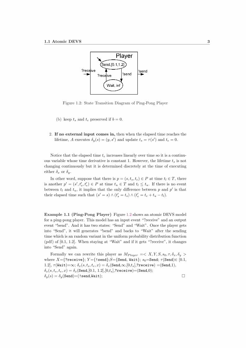
Figure 1.2: State Transition Diagram of Ping-Pong Player
(b) keep ts and te preserved if b = 0.
2. If no external input comes in, then when the elapsed time reaches thelifetime, A executes δy(s) = (y, s′) and update ts = τ(s′) and te = 0.
Notice that the elapsed time te increases linearly over time so it is a continu-ous variable whose time derivative is constant 1. However, the lifetime ts is notchanging continuously but it is determined discretely at the time of executingeither δx or δy.
In other word, suppose that there is p = (s, ts, te) ∈ P at time tl ∈ T , thereis another p′ = (s′, t′s, t
′e) ∈ P at time tu ∈ T and tl ≤ tu. If there is no event
between tl and tu, it implies that the only difference between p and p′ is thattheir elapsed time such that (s′ = s) ∧ (t′s = ts) ∧ (t′e = te + tu − tl).
Example 1.1 (Ping-Pong Player) Figure 1.2 shows an atomic DEVS modelfor a ping-pong player. This model has an input event “?receive” and an outputevent “!send”. And it has two states: “Send” and “Wait”. Once the player getsinto “Send”, it will generates “!send” and backs to “Wait” after the sendingtime which is an random variant in the uniform probability distribution function(pdf) of [0.1, 1.2]. When staying at “Wait” and if it gets “?receive”, it changesinto “Send” again.
Formally we can rewrite this player as MPlayer =< X,Y, S, s0, τ, δx, δy >
where X={?receive}; Y ={!send};S={Send, Wait}; s0=Send; τ(Send)∈ [0.1,1.2], τ(Wait)=∞; δx(s, ts, te, x) = δx(Send,∞,[0,ts],?receive) =(Send,1),δx(s, ts, te, x) = δx(Send,[0.1, 1.2],[0,ts],?receive)=(Send,0);δy(s) = δy(Send)=(!send,Wait); ¤
4 DEVS Formalism and DEVS# code
1.2 Coupled DEVS
The coupled DEVS provides the hierarchical and modular structure necessaryto describe system networks. Formally, a coupled DEVS is defined by
N =< X, Y,D, {Mi}, EIC, ITC, EOC >
where
• X is a set of input events.
• Y is a set of output events.
• D is a set of names of sub-components
• {Mi} is a set of DEVS models where i ∈ D. Mi can be either an atomicDEVS model or a coupled DEVS model.
• EIC ⊆ X × ⋃i∈D
Xi is a set of external input couplings where Xi is the set
of input events of Mi.
• ITC ⊆ ⋃i∈D
Yi ×⋃
i∈D
Xi is a set of internal couplings where Yi is the set of
output events of Mi.
• EOC ⊆ ⋃i∈D
Yi × Y is a set of external output couplings. ¥
Verbal Description of Coupled DEVS Behavior
The coupled DEVS’s behavior is described verbally as follows.
1. When N receives an input event, the coupled DEVS transmits the inputevent to the sub-components through the set of external input couplings.
2. When a sub-component produces its output event, the coupled DEVStransmits the output event to the other sub-components through the setof internal couplings. The coupled DEVS also produces an output eventof N through the set of external output couplings.
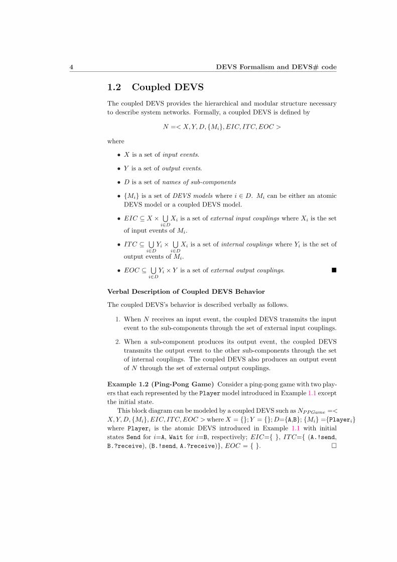
Example 1.2 (Ping-Pong Game) Consider a ping-pong game with two play-ers that each represented by the Player model introduced in Example 1.1 exceptthe initial state.
This block diagram can be modeled by a coupled DEVS such as NPPGame =<
X,Y, D, {Mi}, EIC, ITC, EOC > where X = {};Y = {}; D={A,B}; {Mi} ={Playeri}where Playeri is the atomic DEVS introduced in Example 1.1 with initialstates Send for i=A, Wait for i=B, respectively; EIC={ }, ITC={ (A.!send,B.?receive), (B.!send, A.?receive)}, EOC = { }. ¤
1.3 Building Ping-Pong Game using DEVS# 5
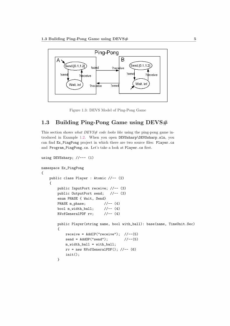
Figure 1.3: DEVS Model of Ping-Pong Game
1.3 Building Ping-Pong Game using DEVS#
This section shows what DEVS# code looks like using the ping-pong game in-troduced in Example 1.2. When you open DEVSsharp\DEVSsharp.sln, youcan find Ex_PingPong project in which there are two source files: Player.cs
and Program_PingPong.cs. Let’s take a look at Player.cs first.
using DEVSsharp; //--- (1)
namespace Ex_PingPong
{
public class Player : Atomic //-- (2)
{
public InputPort receive; //-- (3)
public OutputPort send; //-- (3)
enum PHASE { Wait, Send}
PHASE m_phase; //-- (4)
bool m_width_ball; //-- (4)
RVofGeneralPDF rv; //-- (4)
public Player(string name, bool with_ball): base(name, TimeUnit.Sec)
{
receive = AddIP("receive"); //--(5)
send = AddOP("send"); //--(5)
m_width_ball = with_ball;
rv = new RVofGeneralPDF(); //-- (6)
init();
}
6 DEVS Formalism and DEVS# code
public override void init() { //-- (7)
if (m_width_ball)
m_phase = PHASE.Send;
else
m_phase = PHASE.Wait;
}
public override double tau() //-- (8.a)
{
if (m_phase == PHASE.Send)
return rv.Uniform(0.1, 1.2);
else
return double.MaxValue;
}
public override bool delta_x(PortValue x) //-- (8.b)
{
if (m_phase == PHASE.Wait && x.port == receive)
{
m_phase = PHASE.Send;
return true;
}
else
{
Console.WriteLine("Do we have more than one ball?");
}
return false;
}
public override void delta_y(ref PortValue y) //-- (8.c)
{
if (m_phase == PHASE.Send)
{
y.Set(send);
m_phase = PHASE.Wait;
}
}
public override string Get_s() //-- (9)
{
return m_phase.ToString();
}
}
}
1.3 Building Ping-Pong Game using DEVS# 7
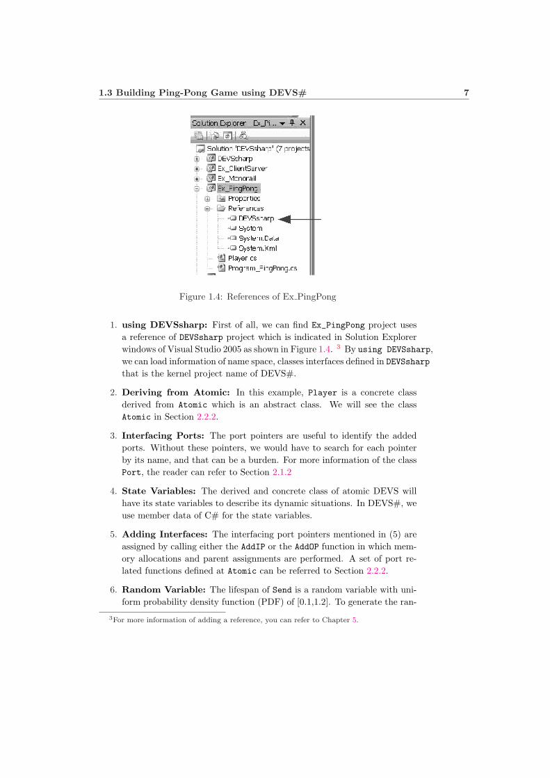
Figure 1.4: References of Ex PingPong
1. using DEVSsharp: First of all, we can find Ex_PingPong project usesa reference of DEVSsharp project which is indicated in Solution Explorerwindows of Visual Studio 2005 as shown in Figure 1.4. 3 By using DEVSsharp,we can load information of name space, classes interfaces defined in DEVSsharp
that is the kernel project name of DEVS#.
2. Deriving from Atomic: In this example, Player is a concrete classderived from Atomic which is an abstract class. We will see the classAtomic in Section 2.2.2.
3. Interfacing Ports: The port pointers are useful to identify the addedports. Without these pointers, we would have to search for each pointerby its name, and that can be a burden. For more information of the classPort, the reader can refer to Section 2.1.2
4. State Variables: The derived and concrete class of atomic DEVS willhave its state variables to describe its dynamic situations. In DEVS#, weuse member data of C# for the state variables.
5. Adding Interfaces: The interfacing port pointers mentioned in (5) areassigned by calling either the AddIP or the AddOP function in which mem-ory allocations and parent assignments are performed. A set of port re-lated functions defined at Atomic can be referred to Section 2.2.2.
6. Random Variable: The lifespan of Send is a random variable with uni-form probability density function (PDF) of [0.1,1.2]. To generate the ran-
3For more information of adding a reference, you can refer to Chapter 5.

8 DEVS Formalism and DEVS# code
dom number, Player defines a random variable rv as a general PDFrandom variable in (4), and pick the uniform PDF in the range[0.1, 1.2]in tau() function in (8.a). The PDFs available in DEVS# are addressedin Section 2.4.
7. The initial State s0: To make the initial state s0, all concrete classesderived from Atomic are supposed to override the function init() in whichthe associated atomic model is reset to the initial state s0. In this case ofPlayer, the initial phase can be determined as Send or Wait depending onanother variable, m_width_ball which is indicating to have a ball initiallyor not.
8. Characteristic Functions τ, δx and δy: all concrete classes derivedfrom Atomic should override the characteristic functions: τ, δx, and δy.
(a) τ of Player returns the random number from [0.1, 1.2] when the stateis Send, otherwise it returns∞ that is represented by double.MaxValue.
(b) δx of Player changes the state Wait to Send when receiving the inputevent receive.
(c) δy of Player generates the output event send, at the same time, itchanges the state Send to Wait.
9. Displaying Status: To show the current state, we will override theGet_s() function which is supposed to return a string representing thecurrent state. Player returns the string value of m_phase variable.
A ping-pong match we are considering here needs two players that are in-stances of the previous class Player. We use the coupled DEVS in Program_PingPong.cs
to model the match as shown in the following codes.
using DEVSsharp;
namespace Ex_PingPong
{
class Program_VM
{
static Devs MakePingPong(string name)
{
Coupled game = new Coupled(name); //-- (1)
Player A = new Player("A", true); //-- (2)
Player B = new Player("B", false);//-- (2)
game.AddModel(A); //-- (3)
1.3 Building Ping-Pong Game using DEVS# 9
game.AddModel(B); //-- (3)
game.AddCP(A.send, B.receive); //-- (4)
game.AddCP(B.send, A.receive); //-- (4)
game.PrintCouplings(); //-- (5)
return game;
}
static void Main(string[] args)
{
Devs md = MakePingPong("PingPong");
SRTEngine Engine = new SRTEngine(md, 10000, null);//--(6)
Engine.RunConsoleMenu();//--(7)
}
}
}
1. Making the Ping-Pong Game as coupled DEVS: We make an in-stance of Coupled in DEVS# for the ping-pong game.
2. Instancing Two Players The ping-pong game has two sub-componentsthat are instances of Player having different initial states.
3. Adding Components We add two players A and B by calling the functionAddModel of the class Coupled.
4. Adding Couplings We add couplings between players A and B callingthe function AddCP of the class Coupled .
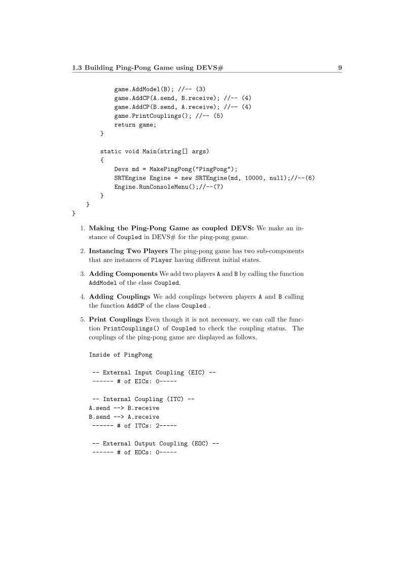
5. Print Couplings Even though it is not necessary, we can call the func-tion PrintCouplings() of Coupled to check the coupling status. Thecouplings of the ping-pong game are displayed as follows.
Inside of PingPong
-- External Input Coupling (EIC) --
------ # of EICs: 0-----
-- Internal Coupling (ITC) --
A.send --> B.receive
B.send --> A.receive
------ # of ITCs: 2-----
-- External Output Coupling (EOC) --
------ # of EOCs: 0-----

10 DEVS Formalism and DEVS# code
6. Making a simulation engine Instancing a scalable simulation engineSRTEngine can be done by calling its constructor that needs the modelsupposed to be simulated. In this example the model is the coupled modelof the ping-pong game, pp. For more detailed information of SRTEngine,the reader can refer to Section 2.3.
7. Running the console menu We can use the console menu of SRTEngineby calling RunConsoleMenu(). After that, we will see the following screenon the selected console.
DEVS#: C# Open Source of DEVS Formalism, (C) 2005~2007,
http://xsy-csharp.sourceforge.net/DEVSsharp/
The current date is 5/6/2007.
The current time is 1:05:52 PM.
scale, step, run, mrun, [p]ause, pause_at, [c]ontinue, reset,
rerun, [i]nject, dtmode, animode, print, cls, log, [e]xit
>
The first part shows the header of DEVS# and current date and time.The second part shows the available command set. Even we don’t haveclear idea of each command, let’s try“ run” and then “exit”.
The detailed information of each command will be provided in Section 2.3.
Chapter 2
Structure of DEVS#
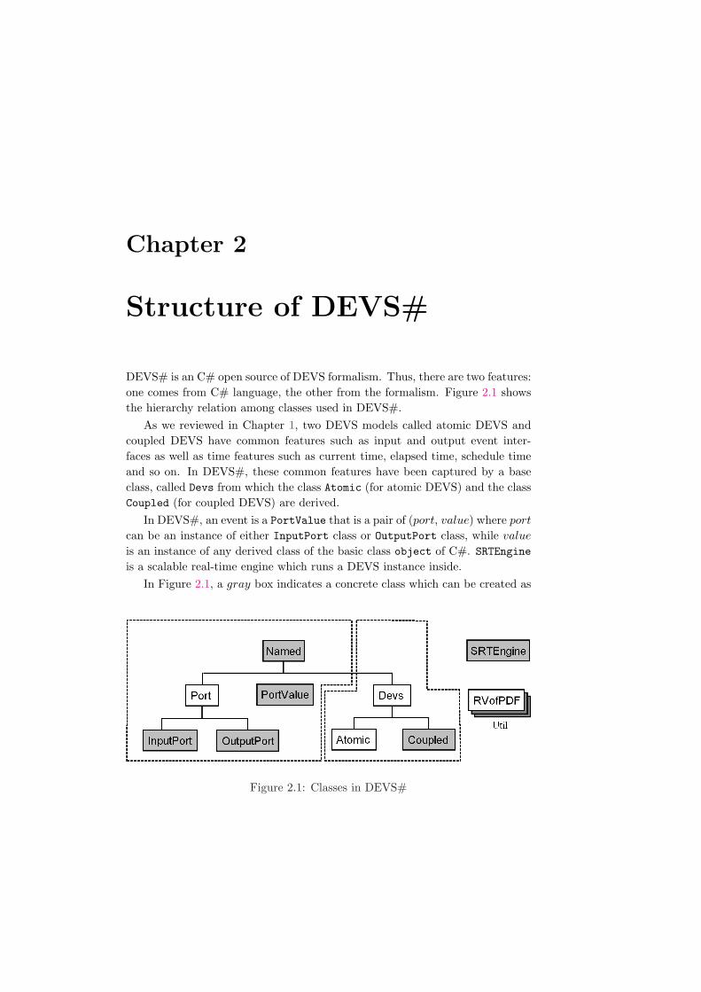
DEVS# is an C# open source of DEVS formalism. Thus, there are two features:one comes from C# language, the other from the formalism. Figure 2.1 showsthe hierarchy relation among classes used in DEVS#.
As we reviewed in Chapter 1, two DEVS models called atomic DEVS andcoupled DEVS have common features such as input and output event inter-faces as well as time features such as current time, elapsed time, schedule timeand so on. In DEVS#, these common features have been captured by a baseclass, called Devs from which the class Atomic (for atomic DEVS) and the classCoupled (for coupled DEVS) are derived.
In DEVS#, an event is a PortValue that is a pair of (port, value) where port
can be an instance of either InputPort class or OutputPort class, while value
is an instance of any derived class of the basic class object of C#. SRTEngineis a scalable real-time engine which runs a DEVS instance inside.
In Figure 2.1, a gray box indicates a concrete class which can be created as
Figure 2.1: Classes in DEVS#
12 Structure of DEVS#
an instance, while a white box is an abstract class which can not be created asan instance.
We will first go through PortValue related classes in Section 2.1. Next,Devs class and its derived two classes: Atomic and Coupled will be investi-gated in Section 2.2. Section 2.3 will introduce a simulation engine class, calledSRTEngine. And finally, we will see the random number generator classes inSection 2.4.
2.1 Event=PortValue
An event will be modeled by an instance of PortValue class which is a pairof Port and Value. We will first see the top-most base class, called “Named”.Then we will look at Port-related classes, and finally, the PortValue class willbe seen in the last part of this section.
2.1.1 Named
Named is defined in Named.cs file as a concrete class. The class provides itsconstructor whose argument is a string, and has a public Name field as a string.The function ToString() is the function overrided from object::ToString().
public class Named
{
public String Name;
public Named(string name)
{
m_Name = name;
}
public override string ToString()
{
return m_name;
}
}
2.1.2 Port, InputPort, and OutputPort
The Port.cs file defines three classes Port, InputPort and OutputPort asfollows.
class Port: public Named
{

2.1 Event=PortValue 13
public Devs Parent;
protected List<Port> m_FromP, // From Ports
m_ToP; // To Ports
public List<Port> FromP { get { return m_FromP; } }
public List<Port> ToP { get { return m_ToP; } }
};
class InputPort: public Port {
...
};
class OutputPort: public Port {
...
};
Port is an abstract class derived from Named. It has Parent field whose typeis Devs, and which is automatically assigned when we call the AddIP() andAddOP() functions of Devs (see Section 2.2). Port has “List<Port> ToP” as aset of successors as well as “List<Port> FromP” as a set of predecessors whichare changed when we call AddCP() and RemoveCP() of Coupled (see Section2.2.3).
InputPort and OutputPort are concrete and derived classes from Port.
2.1.3 PortValue
As mentioned before, an event in DEVS# is modeled by PortValue class thathave a pair of a deriving class of Port and a deriving class of object. Thefollowing codes are parts of PortValue.cs.
class PortValue {
public:
public Port port; //-- either an output or an input port
public object value; // deriving class from the Object class
public PortValue(Port prt){...}
public PortValue(Port prt, object v) {...}
public void Set(Port prt){...}
public void Set(Port prt, object v){...}
public override string ToString(){...}
};
Two constructors and two Set functions are available whose arguments canbe Port p which means value v=null, or a pair of (Port p and object v). The

14 Structure of DEVS#
function ToString() returns the string concatenating of port and value (ifvalue is not null) by using a delimiter ‘:’ character.
2.2 DEVS
As introduced in Chapter 1, DEVS has two basic structures: atomic DEVS andcoupled DEVS. In DEVS#, these two structures are implemented as the classesAtomic and Coupled, respectively, and are derived from the base class Devs.Thus Devs has the common member data and functions of both Atomic andCoupled.
2.2.1 Base DEVS: Devs
Devs defined in the source file Devs.cs is an abstract class derived from Named.Devs points its parent through its Parent field which is assigned by Coupled::AddModel()
(see Section 2.2.3).
public class Devs: Named {
public Coupled Parent; // parent pointer
...
There are adding, getting, removing, and printing functions for the inputports denoted as AddIP, GetIP, RemoveIP, and PrintAllIPs. Similarly, AddOP,GetOP, RemoveOP, and PrintAllOPs are available functions for the output ports.
In addition, IP and OP get the set of input ports as SortedList<string, InputPort>
and the set of output ports as SortedList<string, OutputPort>, respectively.
//-- X port Methods --
InputPort AddIP(string ipn);
InputPort GetIP(string ipn) const;
InputPort RemoveIP(string ipn);
void PrintAllIPs() ;
public SortedList<string, InputPort> IP {get ; }
//-- Y port Methods --
OutputPort AddOP(string opn);
OutputPort GetOP(string opn) const;
OutputPort RemoveOP(string opn);
void PrintAllOPs() ;
public SortedList<string, OutputPort> OP {get ; }
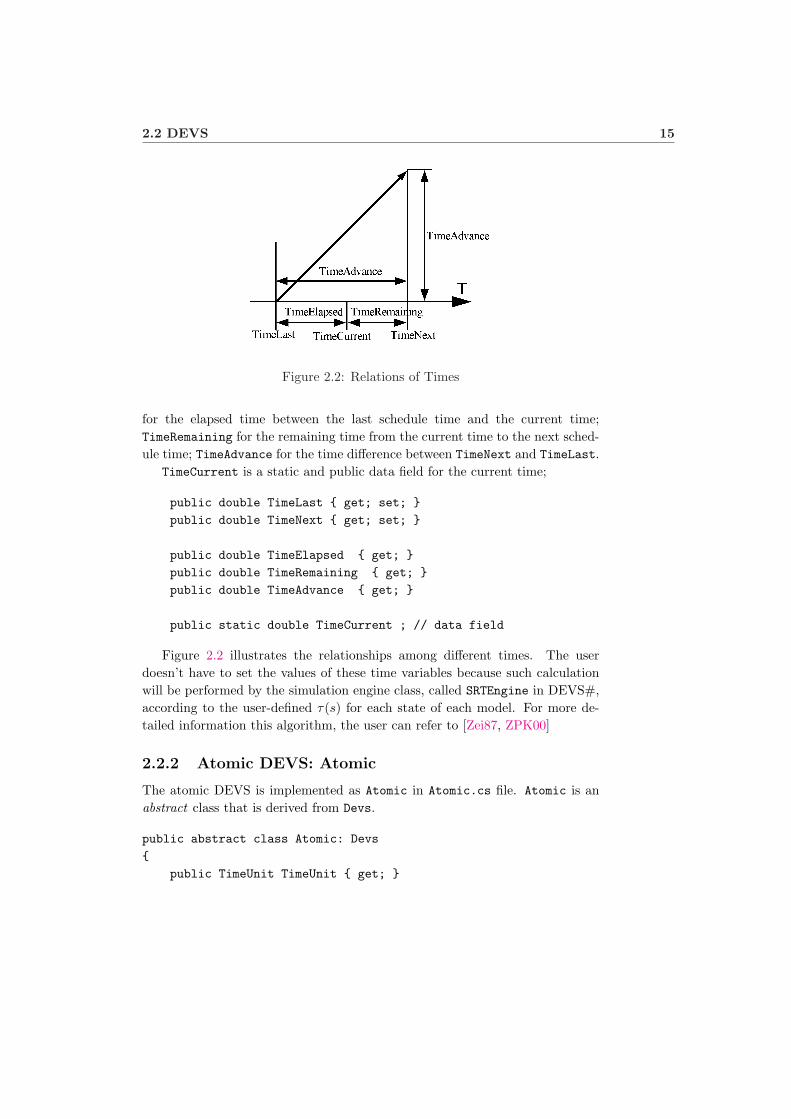
Devs has time-related properties such as TimeLast for getting (or setting) thelast schedule update time; TimeNext for the next schedule time; TimeElapsed
2.2 DEVS 15
Figure 2.2: Relations of Times
for the elapsed time between the last schedule time and the current time;TimeRemaining for the remaining time from the current time to the next sched-ule time; TimeAdvance for the time difference between TimeNext and TimeLast.
TimeCurrent is a static and public data field for the current time;
public double TimeLast { get; set; }
public double TimeNext { get; set; }
public double TimeElapsed { get; }
public double TimeRemaining { get; }
public double TimeAdvance { get; }
public static double TimeCurrent ; // data field
Figure 2.2 illustrates the relationships among different times. The userdoesn’t have to set the values of these time variables because such calculationwill be performed by the simulation engine class, called SRTEngine in DEVS#,according to the user-defined τ(s) for each state of each model. For more de-tailed information this algorithm, the user can refer to [Zei87, ZPK00]
2.2.2 Atomic DEVS: Atomic
The atomic DEVS is implemented as Atomic in Atomic.cs file. Atomic is anabstract class that is derived from Devs.
public abstract class Atomic: Devs
{
public TimeUnit TimeUnit { get; }

16 Structure of DEVS#
public Atomic(string name, TimeUnit ): base(name) {...}
...
An instance of Atomic class has its own time unit. TimeUnit is defined inTimeUnit.cs file as an enumerate type:
public enum TimeUnit { MilliSec, Sec, Min, Hour, Day }.
Therefore, the lifetime of a state s, τ(s) is interpreted in τ(s)∗ TimeUnit in-side DEVS#. However, to handle all different schedules in different time units ofall atomic models used in a simulation run, time conversions are internally donein DEVS#. As a result, TimeLast, TimeNext, TimeElapsed, TimeRemaining,and TimeAdvance will be interpreted in second internally.
Characteristic Functions
There are four public characteristic functions that are defined as abstract inAtomic class. Thus the user must override them to define a concrete class fromAtomic.
The function init() is used when the model needs to be reset to its initialstate s0, such as at the beginning of a simulation run.
public abstract void init();
The function tau() returns the lifespan of the current state when the sched-ule of the next internal event is reset by the time of an interrupting input eventor an generating output event.
public abstract double tau();
The function delta_x(PortValue x) defines the input state transition causedby an input event x. The return value true indicates that the next scheduleneeds to be updated by calling tau(). Contrarily, the return value false indi-cates that the time for the next schedule needs to be preserved.
public abstract bool delta_x(PortValue x) ;
The function delta_y(ref PortValue y) defines the output transition bygenerating an output event y. Recall that the schedule will be updated rightafter this occurs, based upon the value of tau().
public abstract void delta_y(ref PortValue y);
Displaying State as a string
There is an other public virtual(but not abstract) function Get_s(), that issupposed to return the current status in a string for display purpose.
public virtual string Get_s() { return ""; }
2.2 DEVS 17
Collecting Performance Functions
If we want to trace the performance of an atomic DEVS model, we need to set theflag on by using CollectStatistics(true). We can also get the flag’s status bycalling CollectStatisticsFlag(). The virtual function Get_Statistics_s()
is supposed to return a string which represents the status in terms of collectingstatistics. Also, the user can override the GetPerformance() function to collectthe performance index.
public void CollectStatistics(bool flag) { m_cs = flag; }
public bool CollectStatisticsFlag() const { return m_cs; }
public virtual string Get_Statistics_s() const { return Get_s(); }
public virtual Dictionary<string, double> GetPerformance() const;
We will see the theoretical background of performance indices and how we collectthem using DEVS# in Chapter 4.
2.2.3 Coupled DEVS: Coupled
The coupled DEVS is implemented as the class Coupled derived from the classDevs. Coupled class is concrete.
public class Coupled: Devs
{
public Coupled(string name): base(name) {...}
Sub-components Related
There are four functions and one property associated with modeling of sub-components as follows.
public void AddModel(Devs md);
public Devs GetModel(string name);
public void RemoveModel(string name);
public void RemoveAllModels();
public List<Devs> Models { get; }
Couplings Related
Related to couplings, there are three coupling related functions for adding, re-moving, and printing as follows.
public void AddCP(Port spt, Port dpt);
public void RemoveCP(Port spt, Port dpt);
public void PrintCouplings() ;
18 Structure of DEVS#
2.3 Scalable Real-Time Engine: SRTEngine
DEVS# provides a simulation engine class, called SRTEngine. When we makean instance of SRTEngine, its constructor creates an independent simulationthread from the main thread. The reader can find the source codes of SRTEnginein SRTEngine.cs file.
2.3.1 Constructor
SRTEngine(Devs model, double ending_t, Callback call_back);
The constructor needs three arguments: the first argument is the Devs modelto be simulated, the second is the simulation terminating time in second, thelast is a callback function that is used to inject a user-input into the simulationmodel.
The third argument Callback is defined as delegate which can be seen asa function pointer in C#.
public delegate PortValue Callback(Devs model);
Callback is supposed to return a PortValue which represents the user inputto the model. Thus, PortValue’s port should be an input port of Devs model.The following example shows that InjectMsg returns a PortValue whose portis vm’s ip input port.
PortValue InjectMsg(Devs md)
{
VM vm = (VM) md;
return PortValue(vm.ip);
}
Then, we can pass the above function pointer of InjectMsg to an instance ofSRTEngine as follows.
SRTEngine simEngine(vm, 10000, InjectMsg);
We will see another example to use Callback in the example Ex_VendingMachinin Section 3.1.2.
2.3.2 Run console menu
If we call the function RunConsoleMenu() of SRTEngine, it provides a consolemenu as follows.
scale, step, run, mrun, [p]ause, pause_at, [c]ontinue, reset,
rerun, [i]nject, dtmode, animode, print, cls, log, [e]xit
>

2.3 Scalable Real-Time Engine: SRTEngine 19
scale f
scale controls the speed of time flow by the scale factor f
• 0.1 for 10 times slower than real time
• 1 as fast as real time;
• 10 for 10 times faster than real time;
• 0 or greater than 1000,000 for as fast as possible;
The corresponding application programming interfaces (APIs) are:
public double SRTEngine::GetTimeScale();
public void SRTEngine::SetTimeScale(double ts).
step
step executes a simulation run until one internal transition is fired. After thatit pauses the run automatically unless the user inputs commands such as step,continue, run, mrun. This command can be useful when we try a step-by-steprun to see the model behavior. The corresponding API is
public void SRTEngine::Step().
run
run executes a simulation run which continues until it reaches the simulationending time, which is set by the second argument of the SRTEngine constructoror by the command pause_at et. The corresponding API is
public void SRTEngine::MultiRun(unsigned n)
where n=1.
mrun n
mrun executes n simulation runs. Each simulation run stops when it reaches thesimulation ending time. When trying mrun n, where 2≤ n ≤ 20, SRTEinginecalculates the 95% confidence interval of the average values of each statisticalitems. The corresponding API is
public void SRTEngine::MultiRun(unsigned n).
[p]ause
pause or p pauses a simulation run immediately. The corresponding API is
public void SRTEngine::void Pause().

20 Structure of DEVS#
pause at et
pause_at sets the simulation ending time as et. The corresponding APIs are
public double SRTEngine::GetEndingTime() const;
public void SRTEngine::SetEndingTime(double et).
[c]ontinue
continue or c resumes a simulation run which has been paused. It continuesthe previous simulation mode that had been determined by step, run, or mrun.The corresponding API is
public void SRTEngine::Continue().
reset
reset initializes the associated simulation model. The corresponding API is
public void SRTEngine::Reset().
rerun
rerun combines reset and run. The corresponding API is
public void SRTEngine::Rerun().
[i]nject
inject or i injects an user-input event into the simulation model. This com-mand invokes the callback function whose type is PortValue Callback(Devs md)
that is the third argument of the SRTEngine constructor. The correspondingAPI is
public void SRTEngine::Inject(PortValue x).
dtmode
dtmode sets the print mode of discrete transition, both for in the console and inthe log file (whose file name is DEVS#_log.txt). The choice can be one of thefollowing options:
• none displays no discrete state transition.
• te displays the elapsed time TimeElapsed.
• tea displays the elapsed time if associated model’s current state s is active,which means the remaining time TimeRemaining < ∞.

2.3 Scalable Real-Time Engine: SRTEngine 21
• tr displays the remaining time.
• tra displays only an active remaining time.
• nc no change.
The corresponding APIs are
public void SRTEngine::Set_dtmode(PrintStateMode flag, bool ao);
public void SRTEngine::Get_dtmode(ref PrintStateMode flag, ref bool ao).
where
public enum PrintStateMode {P_NONE, P_remaining, P_elapsed}.
animode
animode sets the animation interval. The choice can be either one of the fol-lowing options.
• none displays no animation state transition.
• avi is the number of animation interval > 1.0E-2.
• nc no change.
The related APIs are
public void SRTEngine::SetAnimationFlag(bool flag),
public bool SRTEngine::GetAnimationFlag(),
public void SRTEngine::SetAnimationInterval(double ai),
public double SRTEngine::GetAnimationInterval() const.
print displays information according to the following option.
• q prints the total state of the model.
• cpl prints the couplings information if the model is a coupled DEVS.
• s prints all settings. The following screen shot is made by print s.
scale factor: 1
run-through mode
current time: 0
simulation ending time: 1.79769e+308
current dt_mode: te [(state, t_s, t_e), active only: off]
current animation mode: on and interval= 0.25
current log setting: on, p00

22 Structure of DEVS#
• p prints the performance indices at the current time.
The corresponding APIs are
public void SRTEngine::PrintTotalState() const,
public void SRTEngine::PrintCouplings() const,
public void SRTEngine::PrintSettings() const,
public void SRTEngine::PrintPerformanceOfaRun() const.
cls
cls clears the screen.
log
log sets the logging option which generates the log file DEVS#_log.txt. Afterthe log command, DEVS# shows the current log settings and waits for the userinput as follows.
current log setting: on, p00
options: {on,off}, {+,-}{pqt} nc >
The user options are on or off or {+,-}{pqt} or nc. Their meanings are:
• {on, off} is the main log options. Use on for turning log on or off forturning log off. If the mode is on, three independent options are selectable.
– p is for logging performance indices at the end of a simulation run.
– q is for logging the total state of the model at the end of a simulationrun.
– t is for logging every single discrete event transition.
If all of three are on, it is shown as pqt. If p is on, q and t are off, thedisplay is shown as p00, etc.
• {+,-}{pqt} can be interpreted that + stands for setting the followingoptions on, while - stands for turning the following options off. Forexample +qt means to set q and t on, while -p means to set p off.
• nc no change.
SRTEngine has a public data field of logger which is an instance of Loggerclass. The corresponding APIS of Logger class are
public bool Logger::OnFlag {get; set; },
public bool Logger::TransitionFlag {get; set; },
public bool Logger::PerformanceFlag {get; set; },
public bool Logger::TotalStateFlag {get; set; }.

2.4 Random Variables 23
[e]xit
exit or e exits the console menu.
2.4 Random Variables
2.4.1 Probability Density Functions
Several random variables are provided in DEVS#. All random variable classesare defined in Util\RV.cs. RVofGeneralPDF class generates a random numberof the uniform probability density function (PDF), the triangular PDF, theexponential PDF, and the normal PDF as follows.
public class RVofGeneralPDF: Random
{
public RVofGeneralPDF() : base() { }
public double Uniform(double min, double max);
public double Triangular(double min, double max, double mode);
public double Exponential(double mean);
public double Normal(double mean, double sd);
}
We took a look at the use of RVofGeneralPDF in the ping-pong example inSection 1.3.
If we want to make an instance of a specific PDF’s random variable, we canuse RV_Uniform, RV_Triangular, RV_Exponential, and RV_Normal which arederived classes from an abstract class, RVofPDF. The abstract function RN() ofRVofPDF is overrided in each derived class as follows.
public abstract class RVofPDF : Random
{
protected RVofPDF() : base() { }
public abstract double RN();
}
public class RV_Uniform : RVofPDF
{
protected double min, max;
public RV_Uniform(double _min, double _max): base(){...}
public override double RN(){...} // return Uniform[min,max]
}
public class RV_Triangular : RVofPDF
{
protected double min, max, mode;
24 Structure of DEVS#
public RV_Triangular(double _min, double _max, double _mode): base(){...}
public override double RN(){...} // return Triangular(min,max,mode)
}
public class RV_Exponential : RVofPDF
{
protected double mean;
public RV_Exponential(double _mean): base(){...}
public override double RN(){...} // return Exponential(mean);
}
public class RV_Normal : RVofPDF
{
protected double mean, sd;
public RV_Normal(double _mean, double sd): base(){...}
public override double RN() {...}// return Normal(mean, sd);
}
We will see the use of these PDFs in example in Section ??
2.4.2 Probability Mass Function
A template class RVofPMF<T> is used for generating a random number of a prob-ability mass function (PMF). This class has the probability table pmf which isDictionary<T, double> whose key is T-typed object and value is the proba-bility of occurrence for the key. The function SampleV() returns T-typed keywhose cumulative pmf value is firstly greater than a random number r in uni-form[0, 1].
public class RVofPMF<T> : Random
{
//-- pairs of (T, probability)
public Dictionary<T, double> pmf;
public RVofPMF() : base() {...}
public T SampleV() {...}
}
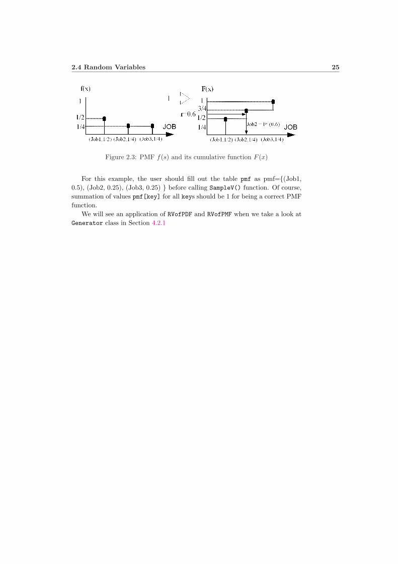
Figure 2.3 shows how RVofPMF::SampleV() works. Let’s assume that thereare three kinds of jobs, Job1, Job2, and Job3 coming into a system with theircorresponding probabilities 0.5, 0.25, and 0.25, respectively. To pick one ofthem, we generate a random number r in the uniform PDF [0, 1]. Let’s sayr = 0.6 at this time. Then, since the inverse function of F (0.6) that is thecumulative function of f(x) is Job2, Job2 will be picked at this moment.
2.4 Random Variables 25
Figure 2.3: PMF f(s) and its cumulative function F (x)
For this example, the user should fill out the table pmf as pmf={(Job1,0.5), (Job2, 0.25), (Job3, 0.25) } before calling SampleV() function. Of course,summation of values pmf[key] for all keys should be 1 for being a correct PMFfunction.
We will see an application of RVofPDF and RVofPMF when we take a look atGenerator class in Section 4.2.1


Chapter 3
Simple Examples
In this chapter, we will see DEVS# examples of atomic DEVS as well as coupledDEVS.
3.1 Atomic DEVS Examples
3.1.1 Timer
An example, Ex_Timer, shows how to define a concrete atomic class fromAtomic. In Timer.cs file, Timer is defined to generat an output op every 3.3seconds as illustrated in Figure 3.1.
Thus Timer has one output port op that is op is assigned by calling AddOP
in the constructor. The function init() does nothing because the class has nointernal variable. The function tau() returns 3.3 all the time.
public class Timer : Atomic
{
private OutputPort op;
public Timer(string name): base(name, TimeUnit.Sec)
{ op = AddOP("op"); init(); }
public override void init(){}
public override double tau() { return 3.3; }
Since there is no input transition defined, delta_x has the null body exceptreturns false 1. However, delta_y returns the output op by making the outputevent y set to op.
1Actually, there is no difference between return false or true in this example.

28 Simple Examples
Figure 3.1: Timer (a) State Transition Diagram (b) Event Segment (c) te Tra-jectory
public override bool delta_x(PortValue x) { return false; }
public override void delta_y(ref PortValue y) { y.Set(op); }
The display function Get_s() returns the current status, which is constantlyWorking.
public override string Get_s() { return "Working"; }
}
The file Program_Timer.cs has the main function for a console applicationas follows. As we can see, we make an instance timer from Timer class. Andthen we make an instance of SRTEngine. Here, we don’t have to pass the thirdCallback function argument because this Timer example doesn’t need the userinput. Finally, this codes run the console menu of SRTEngine class.
class Program
{
static void Main(string[] args)
{
Timer timer = new Timer("STimer");
SRTEngine Engine = new SRTEngine(timer, 10000, null);
Engine.RunConsoleMenu();
}
}
If you try step, you can see the animation is increasing the elapsed time.The following display shows the state at time 2.188 where the schedule timet_s=3.3 and the elapsed time t_e=2.188.
(STimer:Working, t_s=3.300, t_e=2.188) at 2.188
3.1 Atomic DEVS Examples 29
The simulation run will stop at 3.3 because its run mode is step-by-step whenusing step. At that time, it will display the discrete state transition as follows.
(STimer:Working, t_s=3.300, t_e=3.300)
--({!STimer.op},t_c=3.3)-->
(STimer:Working, t_s=3.300, t_e=0.000)
The first state is the source of state transition. An arc shows a triggering eventwhich is the output op of STimer at the current time=3.3. The second state isthe destination of the state transition in which the lifespan is also 3.3 but theelapsed time has been reset to zero.
Exercise 3.1 Consider the example Ex_Timer.
a. Let’s change the display mode from te to tr by applying the commanddtmode. Then preset the simulation ending time to “5” by pause_at 5.Now run until the simulation stops. When it stops at t_c=5, print thetotal state using pinrt with option q. What are the values of t_s andt_r, respectively? Guess the value of t_e at this moment.
b. Add one more state variable int n in Timer class. n should be set = zeroin init(), and it should increase by one in delta_y(). Get_s() shows nin the string format
string.Format("Working, n={0}", n);
3.1.2 Vending Machine
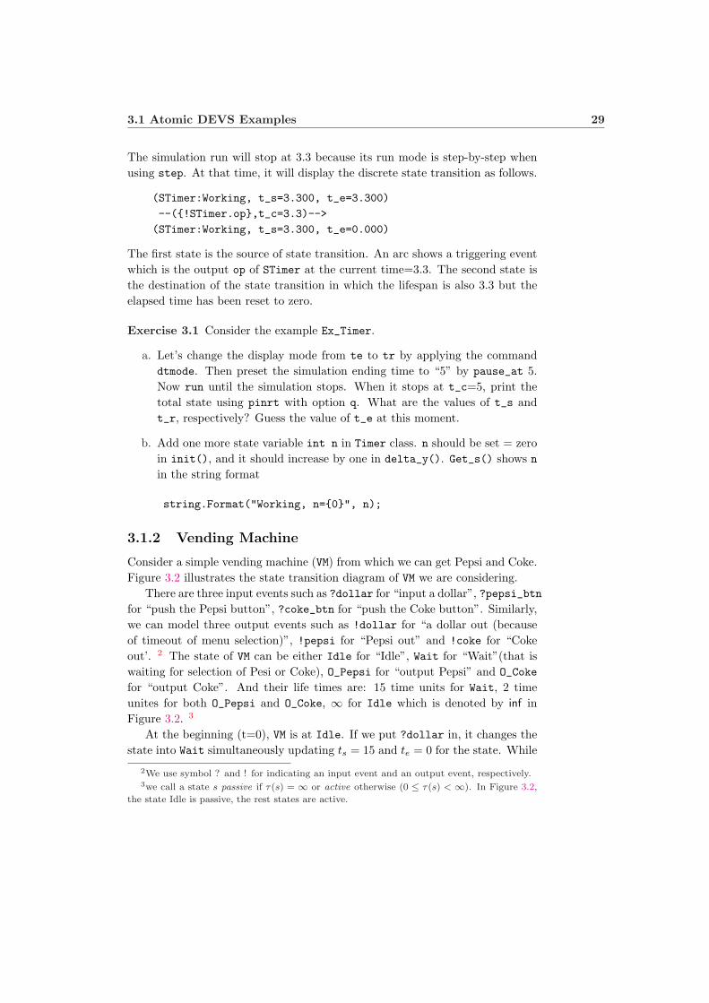
Consider a simple vending machine (VM) from which we can get Pepsi and Coke.Figure 3.2 illustrates the state transition diagram of VM we are considering.
There are three input events such as ?dollar for “input a dollar”, ?pepsi_btnfor “push the Pepsi button”, ?coke_btn for “push the Coke button”. Similarly,we can model three output events such as !dollar for “a dollar out (becauseof timeout of menu selection)”, !pepsi for “Pepsi out” and !coke for “Cokeout’. 2 The state of VM can be either Idle for “Idle”, Wait for “Wait”(that iswaiting for selection of Pesi or Coke), O_Pepsi for “output Pepsi” and O_Coke
for “output Coke”. And their life times are: 15 time units for Wait, 2 timeunites for both O_Pepsi and O_Coke, ∞ for Idle which is denoted by inf inFigure 3.2. 3
At the beginning (t=0), VM is at Idle. If we put ?dollar in, it changes thestate into Wait simultaneously updating ts = 15 and te = 0 for the state. While
2We use symbol ? and ! for indicating an input event and an output event, respectively.3we call a state s passive if τ(s) = ∞ or active otherwise (0 ≤ τ(s) < ∞). In Figure 3.2,
the state Idle is passive, the rest states are active.

30 Simple Examples
Figure 3.2: State Transition Diagram of Vending Machine
in the state, if VM receives ?pepsi_btn (resp. ?coke_btn), it enters into thestate O_Pepsi (resp. O_Coke) and simultaneously updates ts = 2 and te = 0.While in the state O_Pepsi or O_Coke, VM ignores any input and preserves thestate. Similarly, while in the state Wait, VM ignores ?dollar input.
After staying at Wait for 15 time unites, VM returns to Idle state and outputsthe dollar if we don’t select Pepi or Coke within the 15 time units. However, ifwe had selected one of them, VM changes its state into O_Pepsi (resp. O_Coke).Then after 2 time unites, VM outputs !pepsi (resp. !coke) and returns to Idle.
The example of Ex_VendingMachine shows an atomic DEVS model of VMwhich is defined in VendingMachine.cs file. The class VM has three input portidollar, pepsi_btn and coke_btn; three output port odollar, pepsi, coke,all assigned by returning values of the AddIP and AddOP functions in the con-structor.
public class VM : Atomic
{
public InputPort idollar, pepsi_btn, coke_btn;
public OutputPort odollar, pepsi, coke;
enum PHASE { Idle, Wait, O_Pepsi, O_Coke }
PHASE m_phase;
public VM(string name) : base(name, TimeUnit.Sec)
{
idollar = AddIP("dollar");
pepsi_btn = AddIP("pepsi_btn");
coke_btn = AddIP("coke_btn");
odollar = AddOP("dollar");

3.1 Atomic DEVS Examples 31
pepsi = AddOP("pepsi");
coke = AddOP("coke");
init();
}
VM’s initial state is set to Idle in init(). The lifespan of each state is definedin tau() as 15, 2, 2, and ∞ for Wait, O_Pepsi, O_Coke, and Idle, respectively.
public override void init() { m_phase = PHASE.Idle; }
public override double tau()
{
if (m_phase == PHASE.Wait)
return 15;
else if (m_phase == PHASE.O_Pepsi)
return 2;
else if (m_phase == PHASE.O_Coke)
return 2;
else
return double.MaxValue;
}
The input transition function delta_x defines every arc triggered by aninput event in Figure 3.2 and returns true for each such arc. If the input eventidollar arrives while VM is not in state Idle, or if the input events pepsi_btnor coke_btn arrive while VM is not in state Wait, delta_x returns false, andthe input is ignored.
public override bool delta_x(PortValue x)
{
if (m_phase == PHASE.Idle && x.port == idollar)
{
m_phase = PHASE.Wait;
return true; // Reschedule Me
}
else if (m_phase == PHASE.Wait && x.port == pepsi_btn)
{
m_phase = PHASE.O_Pepsi;
return true; // Reschedule Me
}
else if (m_phase == PHASE.Wait && x.port == coke_btn)
{
m_phase = PHASE.O_Coke;
return true; // Reschedule Me
32 Simple Examples
}
return false; // Ignore the input
}
The output transition function delta_y defines every arc generating an outputevent in Figure 3.2.
public override void delta_y(ref PortValue ys)
{
if (m_phase == PHASE.Wait)
ys.Set(odollar);
else if (m_phase == PHASE.O_Pepsi)
ys.Set(pepsi);
else if (m_phase == PHASE.O_Coke)
ys.Set(coke);
m_phase = PHASE.Idle;
}
The virtual function Get_s() is also overridden and returns an m_phase.ToString().
public override string Get_s()
{
return m_phase.ToString();
}
}
Since this vending machine example needs the user input during a simulationrun, we need to define a callback function for the user input. In Program_VM.cs
file, we can see the following static function.
static PortValue InjectMsg(Devs model)
{
if (model is VM)
{
VM vm = (VM)model;
Console.Write("[d]ollar [p]epsi_botton [c]oca_botton > ");
string input = Console.ReadLine();
if (input == "d")
return new PortValue(vm.idollar);
else if (input == "p")
return new PortValue(vm.pepsi_btn);
else if (input == "c")
return new PortValue(vm.coke_btn);
else

3.1 Atomic DEVS Examples 33
{
Console.WriteLine("Invalid input! Try again!");
return new PortValue(null,null);
}
}
else
throw new Exception("Invalid Model!");
}
The callback function InjectMsg casts the type of md from Devs to VM. Andthe user-input of either d, p, or c is mapped to PortValue(vm.idollar),PortValue(vm.pepsi_btn), or PortValue(vm.coke_btn), respectively.
The last part the the code in Program_VM.cs runs the simulation engine.First we make vm as an instance of VM, and plug vm into an instance of SRTEnginewith the simulation ending time=10000 using the above callback function.
static void Main(string[] args)
{
VM vm = new VM("VM");
SRTEngine Engine = new SRTEngine(vm, 10000, InjectMsg);
Engine.RunConsoleMenu();
}
Let’s try the command step. Observe that since the initial state s0 of VMis Idle and its lifespan tau(Idle)=∞, and the initial schedule is also t_s=∞.In this case, the elapsed time t_e cannot ever reach t_s. Thus this commandstep doesn’t stop until te becomes 1000 which is the simulation ending time(unless the user interrupts the simulation).
In this case, we can stop the simulation run using pause or p command,followed by Enter key. The following screen shows the situation if we make itpause at 8.859.
(VM:Idle, t_s=inf, t_e=8.859) at 8.859
Let’s try inject or i. Then we can see the console output which is producedby the above InjectMsg(Devs md) as follows.
[d]ollar [p]epsi_botton [c]oca_botton >
If we input d, we can see the input causes the state to transition from Idle toWait as follows.
(VM:Idle, t_s=inf, t_e=8.859)
--({?dollar,?VM.dollar}, t_c=8.859)-->
(VM:Wait, t_s=15.000, t_e=0.000)
34 Simple Examples
Figure 3.3: Monorail System
Now, we use continue or c to resume stepping again. If we want to pauseagain and inject a menu selection such as pepsi_btn or coke_btn, we can dothat just like before.
Exercise 3.2 Consider modifying the VM model in EX_VendingMachine in orderto add the behavior of rejecting a second dollar input when VM is the state Wait.To model this, let’s add a state Reject whose lifespan is 0. We define the outputtransition δy at Reject as delta_y(Reject) = (!dollar, Wait). Howeverthere are two ways of rescheduling of t_s and t_e of the the state Wait whenVM comes back to the state. Let’s try each of the following two ways.
1. Reset t_s=15 and t_e=0.
2. Return t_s and t_e to the values they had right before the input of theadditional dollar.
3.2 Coupled DEVS Examples
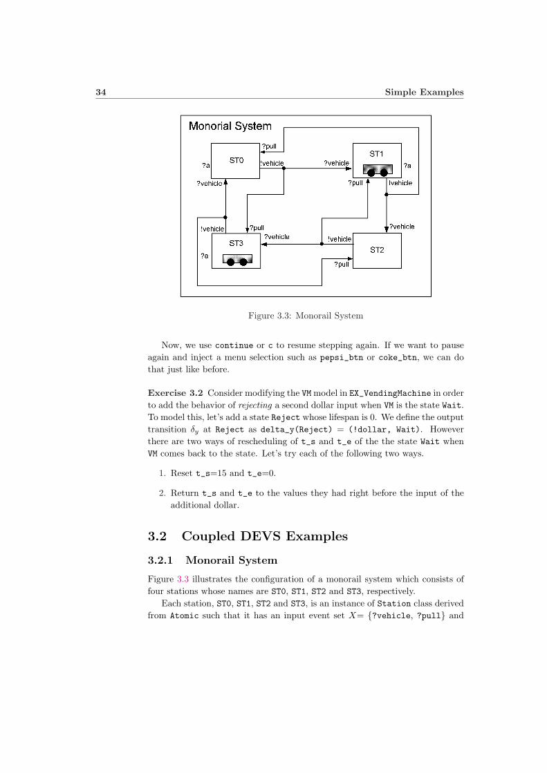
3.2.1 Monorail System
Figure 3.3 illustrates the configuration of a monorail system which consists offour stations whose names are ST0, ST1, ST2 and ST3, respectively.
Each station, ST0, ST1, ST2 and ST3, is an instance of Station class derivedfrom Atomic such that it has an input event set X= {?vehicle, ?pull} and

3.2 Coupled DEVS Examples 35
Figure 3.4: Phase Transition Diagram of Station(A dashed line indicates δx(s, ts, te, x) = (s′, 0).)
an output event set Y ={!vehicle, !pull} and two state variables: phase ∈{Empty (E), Loading (L), Sending (S), Waiting (W), Collided (C)}, and nso ∈{false(f), true(t)} indicating “next station is NOT occupied” for nso=f or “nextstation is occupied” for nso=t.
To avoid collisions that can occur when more than one vehicle attempts tooccupy a station (let’s call it A) at the same time, the station prior to A (let’scall it B) should dispatch the vehicle ONLY when B’s nso = f. The phasetransition diagram of a single station is shown in Figure 3.4 where an arc isaugmented by (pre-condition),(post-condition). For example, when a stationreceives ?p at phase=E, it makes nso=f; if phase=L and nso=f, then when itreceives ?p, it changes into phase=S internally without any output indicated by!φ. The symbols ?v, ?p, and !v in Figure 3.2 stand for ?vehicle, ?pull, and!vehicle, respectively.
The loading time lt is assigned as lt = 10 for ST0, ST2, ST3; lt = 30 for ST1(because ST1 is bigger than the rest other three stations). The initial state foreach station is s0 = (E, t) for ST0 and ST2, s0 = (L, f) for ST1 and ST3.
To model and simulate this monorail system, we build Station as follows.
Station
First of all, a macro REMEMBERING in the first line in Station.cs file is definedfor testing the effect of monitoring the next station’s status using nso.
#define REMEMBERING // for testing the effect of using nso
36 Simple Examples
The class Station has several state variables: m_phase being one of enumPHASE {Sending, Empty, Loading, Waiting, Collided}; bool init_occupiedindicating the initial occupation state of the station, bool nso indicating if thenext station is occupied or not; and the constant variable double loading_t
indicating the lifespan of a state when its phase is Loading.Station has two input port ipull and ivehicle, one output port ovehicle.
These variables, including ports, are assigned in the constructor as follows.
public class Station: Atomic
{
enum PHASE {Sending, Empty, Loading, Waiting, Collided}
PHASE m_phase;
readonly bool init_occupied;
bool nso; //next_state_occpied
readonly double loading_t;
public InputPort ipull, ivehicle;
public OutputPort ovehicle;
public Station(string name, bool occupied, double lt):
base(name, TimeUnit.Sec)
{
init_occupied =occupied;
loading_t = lt;
nso =true;
ipull = AddIP("pull"); ivehicle = AddIP("vehicle");
ovehicle = AddOP("vehicle");
init();
}
Station::init() initializes m_phase depending on init_occupied suchthat m_phase = Sending if init_occupied is true, otherwise, m_phase =Empty.
public override void init()
{
if(init_occupied == true)
m_phase = PHASE.Sending;
else
m_phase = PHASE.Empty;
}

3.2 Coupled DEVS Examples 37
Station::::tau() returns the lifespan of each state; 10 for Sending; loading_tfor Loading; ∞ otherwise.
public override double tau()
{
if (m_phase == PHASE.Sending)
return 10;
else if (m_phase == PHASE.Loading)
return loading_t;
else
return double.MaxValue;
}
Station::delta_x defines the input transition such that if it receives an inputthrough ipull, it marks nso = false which means that “the next station is notoccupied any more”. At that time, if the station’s phase is Waiting, delta_xthen changes the phase to Sending. To remember the next station be occupiedby this Sending action, Station::delta_x sets nso=tru and returns true.
When a station receives a vehicle through ivehicle port, if phase is Empty,its phase changes into Loading; otherwise the phase changes into Collided.
public override bool delta_x(PortValue x)
{
if( x.port == ipull) {
nso = false;
if (m_phase == PHASE.Waiting)
{
#if REMEMBERING
nso = true;
#endif
m_phase = PHASE.Sending;
return true;
}
}
else if(x.port == ivehicle) {
if(m_phase == PHASE.Empty)
m_phase = PHASE.Loading;
else // rest cases lead to Colided!
m_phase = PHASE.Collided;
return true;
}
return false;
}
38 Simple Examples
Station::delta_y defines the output transition behavior such that, at the endof Loading phase, if nso=true, then delta_y changes the stations’ phase intoWaiting. But if nso=false, delta_y marks nso=true for remembering the nextstation’s occupation and changes the station’s phase to Sending. At the endof Sending phase, it sends out the vehicle through ovehicle port and changesthe station’s phase to Empty.
public override void delta_y(ref PortValue y)
{
if (m_phase == PHASE.Loading)
{
if(nso == true)
m_phase = PHASE.Waiting;
else {
#if REMEMBERING
nso = true;
#endif
m_phase = PHASE.Sending;
}
}
else if (m_phase == PHASE.Sending)
{
y.Set(ovehicle);
m_phase = PHASE.Empty;
}
}
The displaying function Get_s() is overridden to return a string containinginformation about m_phase and nso as follows.
public override string Get_s()
{
return string.Format("phase= {0}, nso= {1}", m_phase, nso);
}
Monorail System
To construct the monorail system, we will make four instances from Station
as shown in Program_Monorail.cs file. Stations ST1 and ST3 each have onevehicle initially, the other two have none, while the loading time of ST1 is 30time-units, the other three each have a loading time of 10.
Each station will collect its own performance data. All couplings are con-nected as shown in Figure 3.3. The ending time of simulation is 1000, and thereis no callback function used here.
3.2 Coupled DEVS Examples 39
static Coupled MakeMonorail(string name)
{
Coupled monorail = new Coupled(name);
Station ST0 = new Station("ST0", false, 10);
ST0.CollectStatistics(true);
monorail.AddModel(ST0);
Station ST1 = new Station("ST1", true, 30);
ST1.CollectStatistics(true);
monorail.AddModel(ST1);
Station ST2 = new Station("ST2", false, 10);
ST2.CollectStatistics(true);
monorail.AddModel(ST2);
Station ST3 = new Station("ST3", true, 10);
ST3.CollectStatistics(true);
monorail.AddModel(ST3);
//-------- Add internal couplings ------------
monorail.AddCP(ST0.ovehicle, ST1.ivehicle);
monorail.AddCP(ST1.ovehicle, ST0.ipull);
monorail.AddCP(ST1.ovehicle, ST2.ivehicle);
monorail.AddCP(ST2.ovehicle, ST1.ipull);
monorail.AddCP(ST2.ovehicle, ST3.ivehicle);
monorail.AddCP(ST3.ovehicle, ST2.ipull);
monorail.AddCP(ST3.ovehicle, ST0.ivehicle);
monorail.AddCP(ST0.ovehicle, ST3.ipull);
//---------------------------------------------
return monorail;
}
static void Main(string[] args)
{
Coupled ms = MakeMonorail("mr");
SRTEngine Engine = new SRTEngine(ms, 1000, null);
Engine.RunConsoleMenu();
}

40 Simple Examples
If you try the command run, DEVS# will simulate system performance untilit reaches the simulation ending time of 1000 time units. The default simulationspeed of DEVS# is the real time so it will take 1000 seconds in reality. However,the user don’t have to wait until the simulation ending time. Don’t forget touse the command pause to stop a simulation run any time you want.
We can change the simulation speed as maximum by scale 0 . If you don’tcare of animation output, you can set animode none. In addition, if you don’twant to see the status of discrete state transitions, you can set dtmode none
too.When the simulation stops, DEVS# makes the beep sounds every 1 second.
To stop the beep sounds, input RETURN key (two times it is kind of bugs butI could not fix it yet). The following screen is the results of the command print
p.
mr.ST0
phase= Empty, nso= True: 0.590
phase= Empty, nso= False: 0.000
phase= Loading, nso= False: 0.010
phase= Sending, nso= True: 0.200
phase= Loading, nso= True: 0.190
phase= Waiting, nso= True: 0.010
mr.ST1
phase= Sending, nso= False: 0.010
phase= Empty, nso= False: 0.020
phase= Loading, nso= False: 0.400
phase= Sending, nso= True: 0.190
phase= Empty, nso= True: 0.190
phase= Loading, nso= True: 0.190
mr.ST2
phase= Empty, nso= True: 0.400
phase= Loading, nso= True: 0.000
phase= Loading, nso= False: 0.200
phase= Sending, nso= True: 0.200
phase= Empty, nso= False: 0.200
mr.ST3
phase= Sending, nso= False: 0.010
phase= Empty, nso= False: 0.210
phase= Loading, nso= False: 0.200
phase= Sending, nso= True: 0.190
3.2 Coupled DEVS Examples 41
phase= Empty, nso= True: 0.390
The performance index for each station is the ratio of the total time the stationstays in each state divided by the simulation run time of 1000. In the exampleabove, for mr.ST3, phase= Loading, nso= False: 0.200 indicates that thetotal time ST3 spent in the Loading state was about 20% of the length ofsimulation run time of 1000. That means that station 3 spent about 200 time-units in the Loading phase.
It is not hard to find that since ST1::loading_t=30 is three times longerthan other stations’ loading_t, ST1 stays at Loading about 59% (phase=Loading, nso= False: 0.400 and phase= Loading, nso= True: 0.190). Thiscauses ST0 to transition into Wait because ST1 stays so long at Loading.
Exercise 3.3 Let’s comment out the line of “#define REMEMBERING” in Station.cs
of Ex_Monorial example. Build it again and try run. When the run stops, tryprint q and print p. Is there a station which gets into Collided?


Chapter 4
Performance Evaluation
This section introduces several performance indices in Section 4.1 and showshow to calculate them in Section 4.2.
4.1 Performance Measures
This section introduces four performance indices: Throughput, Cycle Time,Utilization, and Average Queue Length.
4.1.1 Throughput
It is not hard to imagine that a system produces products. In this context,we can think of a performance index for the system that answers the question“how may products does this system produce?” This performance index canbe measured by counting the number of products produced by the system overparticular time period.
If we have x ∈ N jobs produced by the system over an observational timespan to, then the system throughput thrp is
thrp =x
to(4.1)
and its unit of measurement is jobs/time-unit.
Example 4.1 (Throughput) If the number of products produced by a system is2500 during 100 minutes, then its throughput is thrp = 2500/100 = 25 jobs/min.¤

44 Performance Evaluation
Figure 4.1: A System having a Buffer and a Processor
4.1.2 Cycle Time
A system performs a set of activity cycles so its performance can be measuredby how long it has taken to perform an activity cycle. The unit of this measureis time-unit/activity.
Suppose that an activity consists of two events such that one begins at tl andthe other ends at tu. Then the activity duration is tu − tl. If we have activitydata as a set of time pairs A = {(tli, tui)|tli ≤ tui} where i is in some index set,N = {1, 2, . . . , n}, then the (average) cycle time is
tcyc(A) =
∑i∈N
(tui − tli)
n. (4.2)
Cycle time can be interpreted in different contexts. For example, in thesystem which consists of a buffer and a processor as shown in Figure 4.1, thesystem time can be measured over the entire processing activity from arrival todeparture of the BufferProcessor system. Also waiting time can be consideredas the time duration for the waiting activity in Buffer, while processing timecan be the time duration between arrival to and departure from Processor.
Example 4.2 (Cycle Time as System Time) Assume we have the set of timepairs A = {(5, 17), (7, 29), (15, 41), (50, 62)} from arrival to departure of theBufferProcessor system in Figure 4.1. Then the system time is tcyc(A) =(12 + 21 + 26 + 12)/4 = 17.75. ¤
4.1.3 Utilization
Conventionally the definition of utilization is the percentage of the working timeof a machine compared to its total running time. Let’s consider a processor P asshown in Figure 4.2(a) which has two states: Busy, which is defined as workingtime, and Idle, which is defined as “running, but not working” time. Onceit receives an input ?x, it processes the input and then generates output !y

4.1 Performance Measures 45
Figure 4.2: State Trajectory of a Processor
Figure 4.3: A State Trajectory of Vending Machine
after 10 time units. Figure 4.2(b) illustrates a state trajectory of the processorterminating at to = 30. In this trajectory, the total time span of Busy is(15-5)+(30-23)=17, so utilization of the processor is 56.7%=(17/30)*100, whileidle’s percentage is 100-56.7=43.3%.
We can generalize this concept to more than two states. Let’s consider thevending machine introduced in Section 3.1.2. Suppose that we have a statetrajectory of the vending machine as shown in Figure 4.3. This state trajectorycan be seen as a sequences of piece-wise constant segments. The time it takesto transition between states is assumed to be zero.
The time duration of a piece-wise constant segment is defined by td : S×N→T where N is a set of natural numbers. This function maps from state s andthe order i ∈ N of a segment piece to a time span value if the segment piecein the state s, otherwise the value is 0. For example, in the state trajectory ofFigure 4.3, td(Idle, 1) = 5 − 0 = 5, while td(Idle, 2) = 0 because the state ofthe second segment is Wait.
Let C be the current state. Then the probability that the current state iss ∈ S over time from 0 to to, denoted by P (C = s), is
P (C = s) =
∑i∈N
td(s, i)
to. (4.3)

46 Performance Evaluation
It is true that ∑
s∈S
∑
i∈N
td(s, i) = to. (4.4)
So it is also true that
∑
s∈S
P (C = s) =∑
s∈S
∑i∈N
td(s, i)
to
=
toto
= 1. (4.5)
Example 4.3 Consider the state trajectory of Figure 4.3. Then P (C =Idle)= (5+3+10)/40 = 0.45, P (C=Wait) = (15+5)/40 =0.5, P (C=O_pepsi)=2/40=0.05, P (C=O_coke)=0. ¤
Exercise 4.1 Assume that we have a processor as shown in Figure 4.2(a). Fromthe processor, we have an event segment ω[0,50] = (?x, 10)(!y, 20)(?x, 35)(!y, 45)where (z, t) means an event z occurs at t ∈ T and the observation was performedfrom 0 to 50. Calculate P (C=Idle) and P (C=Busy) over time [0,50]. ¤
To calculate P (C = s), we need to keep track of∑i
td(s, i) by accumulating all
time durations of piece-wise constant time segments when the system is in states. We will see how to implement this in Section 4.2.2.
4.1.4 Average Queue Length
Once again, let’s consider a system with a buffer and a processor that areserially connected as shown in Figure 4.1. To avoid collisions of multiple inputsat the processor, the buffer stores inputs while the processor is busy working onprevious inputs.
Depending on inter-arrival times of between inputs and Processor’s process-ing time, the length of time an input waits in Buffer can vary widely. Thusthe number of waiting inputs (queue size) can be a random number.
Recall how we developed the probability that the current state C is equalto a state s in Section 4.1.3. Let the current state C of Buffer be defined asthe number of inputs currently waiting in buffer. Then the probability that thenumber of waiting parts C is equal to x ∈ N, where N is a suitably definedsubset of the natural numbers, over an observation time from 0 to to is
P (C = x) =
∑i∈N
td(x, i)
to(4.6)
The mean or expected value of C is defined by
E(C) =∑
x∈NxP (C = x) (4.7)
The Average Queue Length is defined as Equation (4.7).
4.1 Performance Measures 47
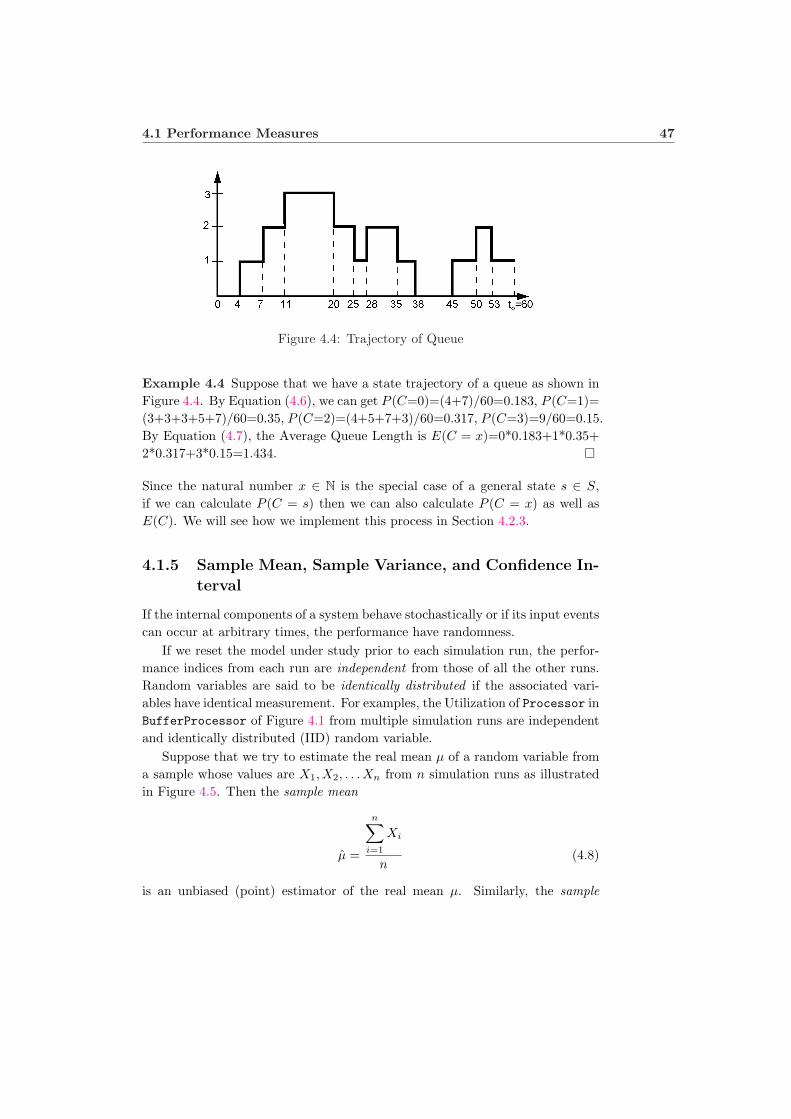
Figure 4.4: Trajectory of Queue
Example 4.4 Suppose that we have a state trajectory of a queue as shown inFigure 4.4. By Equation (4.6), we can get P (C=0)=(4+7)/60=0.183, P (C=1)=(3+3+3+5+7)/60=0.35, P (C=2)=(4+5+7+3)/60=0.317, P (C=3)=9/60=0.15.By Equation (4.7), the Average Queue Length is E(C = x)=0*0.183+1*0.35+2*0.317+3*0.15=1.434. ¤
Since the natural number x ∈ N is the special case of a general state s ∈ S,if we can calculate P (C = s) then we can also calculate P (C = x) as well asE(C). We will see how we implement this process in Section 4.2.3.
4.1.5 Sample Mean, Sample Variance, and Confidence In-
terval
If the internal components of a system behave stochastically or if its input eventscan occur at arbitrary times, the performance have randomness.
If we reset the model under study prior to each simulation run, the perfor-mance indices from each run are independent from those of all the other runs.Random variables are said to be identically distributed if the associated vari-ables have identical measurement. For examples, the Utilization of Processor inBufferProcessor of Figure 4.1 from multiple simulation runs are independentand identically distributed (IID) random variable.
Suppose that we try to estimate the real mean µ of a random variable froma sample whose values are X1, X2, . . . Xn from n simulation runs as illustratedin Figure 4.5. Then the sample mean
µ̂ =
n∑
i=1
Xi
n(4.8)
is an unbiased (point) estimator of the real mean µ. Similarly, the sample
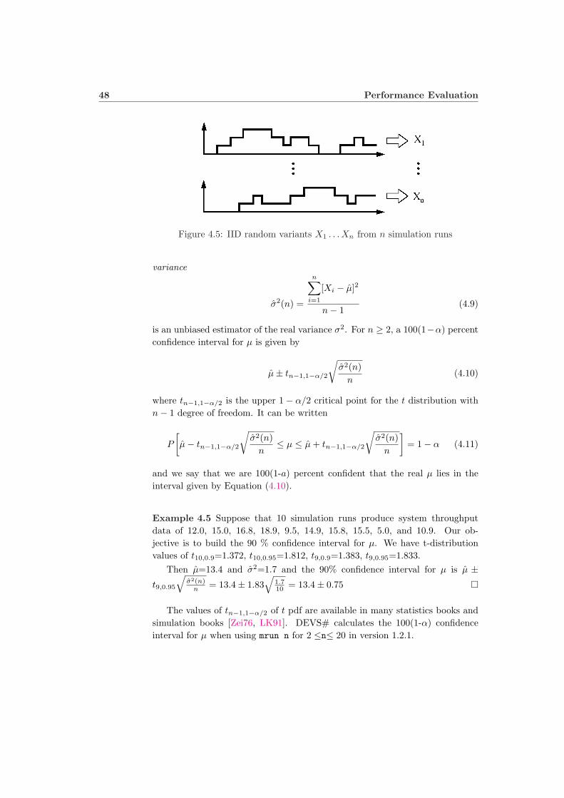
48 Performance Evaluation
Figure 4.5: IID random variants X1 . . . Xn from n simulation runs
variance
σ̂2(n) =
n∑
i=1
[Xi − µ̂]2
n− 1(4.9)
is an unbiased estimator of the real variance σ2. For n ≥ 2, a 100(1−α) percentconfidence interval for µ is given by
µ̂± tn−1,1−α/2
√σ̂2(n)
n(4.10)
where tn−1,1−α/2 is the upper 1− α/2 critical point for the t distribution withn− 1 degree of freedom. It can be written
P
[µ̂− tn−1,1−α/2
√σ̂2(n)
n≤ µ ≤ µ̂ + tn−1,1−α/2
√σ̂2(n)
n
]= 1− α (4.11)
and we say that we are 100(1-a) percent confident that the real µ lies in theinterval given by Equation (4.10).
Example 4.5 Suppose that 10 simulation runs produce system throughputdata of 12.0, 15.0, 16.8, 18.9, 9.5, 14.9, 15.8, 15.5, 5.0, and 10.9. Our ob-jective is to build the 90 % confidence interval for µ. We have t-distributionvalues of t10,0.9=1.372, t10,0.95=1.812, t9,0.9=1.383, t9,0.95=1.833.
Then µ̂=13.4 and σ̂2=1.7 and the 90% confidence interval for µ is µ̂ ±t9,0.95
√σ̂2(n)
n = 13.4± 1.83√
1.710 = 13.4± 0.75 ¤
The values of tn−1,1−α/2 of t pdf are available in many statistics books andsimulation books [Zei76, LK91]. DEVS# calculates the 100(1-α) confidenceinterval for µ when using mrun n for 2 ≤n≤ 20 in version 1.2.1.

4.2 Practice in DEVS# 49
4.2 Practice in DEVS#
This section addresses how we can calculate the performance indices usingDEVS#. All classes used in this section are available in DEVSsharp/ModelBase/
folder.
4.2.1 Throughput and System Time in DEVS#
Throughput can be collected by counting flow entities coming out of the systemunder study, while System Time can be collected by tracing the arrival time andthe departure time of each flow entity. 1 ModelBase library provides a basicclass for flow entities, called the class Job in Job.cs file.
Job
Job class has public data fields: int type, int id and Dictionary<string, double> TimeMap.TimeMap will be used for stamping a pair of an event string and its occurrencetime (we will see examples in Generator class and Transducer class later).
There are tree constructors, a string conversion function ToString(). Thevirtual function, Clone() is supposed to return a clone of this class instance.
public class Job
{
public int type;
public int id;
public Dictionary<string, double> TimeMap;
public Job(int Type) {...}
public Job(int Type, int Id){...}
public Job(Job ob) { ... }
public override string ToString();
public virtual Job Clone() { return new Job(this); }
}
To generate and to collect instances of Job class, we will use two atomicmodels: Generator in Generator.cs and Transducer in Transducer.cs, whichare key models in the experimental frame. For collecting System Time, we willneed the cooperation of both Generator and Transducer.
1Flow entities can be clients of a bank, products of a manufacturing system, airplanes of
an airport, and messages of a communicating network.
50 Performance Evaluation
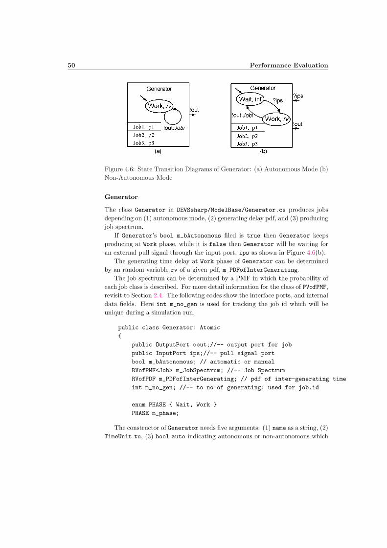
Figure 4.6: State Transition Diagrams of Generator: (a) Autonomous Mode (b)Non-Autonomous Mode
Generator
The class Generator in DEVSsharp/ModelBase/Generator.cs produces jobsdepending on (1) autonomous mode, (2) generating delay pdf, and (3) producingjob spectrum.
If Generator’s bool m_bAutonomous filed is true then Generator keepsproducing at Work phase, while it is false then Generator will be waiting foran external pull signal through the input port, ips as shown in Figure 4.6(b).
The generating time delay at Work phase of Generator can be determinedby an random variable rv of a given pdf, m_PDFofInterGenerating.
The job spectrum can be determined by a PMF in which the probability ofeach job class is described. For more detail information for the class of PVofPMF,revisit to Section 2.4. The following codes show the interface ports, and internaldata fields. Here int m_no_gen is used for tracking the job id which will beunique during a simulation run.
public class Generator: Atomic
{
public OutputPort oout;//-- output port for job
public InputPort ips;//-- pull signal port
bool m_bAutonomous; // automatic or manual
RVofPMF<Job> m_JobSpectrum; //-- Job Spectrum
RVofPDF m_PDFofInterGenerating; // pdf of inter-generating time
int m_no_gen; //-- to no of generating: used for job.id
enum PHASE { Wait, Work }
PHASE m_phase;
The constructor of Generator needs five arguments: (1) name as a string, (2)TimeUnit tu, (3) bool auto indicating autonomous or non-autonomous which

4.2 Practice in DEVS# 51
is assign to the internal variable m_bAutonomous, (4) InterGenerating PDF asRVofPDF, and (5) Job spectrum as RVofPMF<Job> as follows.
public Generator(string name, TimeUnit tu, bool auto, RVofPDF InterGenerating,
RVofPMF<Job> JobSelection):base(name,tu){...}
Generator::init() resets m_no_gen to zero. m_phase is set to Work ifm_bAutonomous is true, otherwise, it is set to Wait. If m_JobSpectrum is notnull m_statistics is initialized by each type of job available in m_JobSpectrum.m_statistics of Generator will collect statistics how may jobs have been
produced.
public override void init()
{
m_no_gen = 0; //
if (m_bAutonomous)
m_phase = PHASE.Work;
else
m_phase = PHASE.Wait;
if (m_JobSpectrum != null)
{
foreach (Job job in m_JobSpectrum.pmf.Keys)
m_statistics.Add(job.type.ToString(), 0.0);
}
}
When the phase of Generator is Work, Generator::tau() returns a randomvalue from the pdf m_PDFofInterGenerating(which is set through the construc-tor function of Generator). If Generator’s phase is Wait, it returns the infinityas the lifespan of Wait.
public override double tau()
{
if (m_phase == PHASE.Work)
{
double t = m_PDFofInterGenerating.RN();
return t;
}else // PHASE.Wait
return double.MaxValue;
}
Generator::detla_x() treats the situation that Generator is non-autonomous,and it receives the pull signal through ips port when it waits for the signal.Otherwise, Generator ignores any input signal.

52 Performance Evaluation
public override bool delta_x(PortValue x)
{
if (m_bAutonomous == false && x.port == ips &&
m_phase == PHASE.Wait)
{
m_phase = PHASE.Work;
return true;
}
return false;
}
In Generator::detla_y(), Generator has a non-trivial m_JobSpectrum ,Generator picks one job by calling m_JobSpectrum.SampleV() and clones thepicked job to clnt. The unique job id for clnt is assigned. At this time,Generator stamps the current time into clnt’s TimeMap with its key value asthe string “SysIn”. This event time will be used when collecting System TimePerformance Index by Transducer that we will look through later.
To collect of how many different jobs are generated, Generator accumulatesthe number of jobs generated with respect to their job types.
After generating a job (or null job) through oout port, if Generator is non-autonomous, it goes back to the phase Wait, otherwise it keep generating thenext job by staying its phase Work.
public override void delta_y(ref PortValue y)
{
if (m_JobSpectrum != null && m_JobSpectrum.pmf.Count > 0)
{
Job clnt = (m_JobSpectrum.SampleV()).Clone();
clnt.id = ++m_no_gen;
//-- (event, time) stamping
clnt.TimeMap.Add("SysIn", Devs.TimeCurrent);
y.Set(oout, clnt);
m_statistics[clnt.type.ToString()] += 1;
}
else // no job value sent
y.Set(oout);
if (m_bActive == false)
m_phase = PHASE.Wait;
}

4.2 Practice in DEVS# 53
Figure 4.7: State Transition Diagrams of Transducer
Transducer
Transducer’s behavior is pretty much opposite to that of Generator. Figure4.7 shows its state transition diagram. It has an input port iin and a bufferCollector as Dictionary<int, List<Job>> to collect jobs coming in withrespect to their types.
public class Transducer: Atomic
{
public InputPort iin;
Dictionary<int, List<Job>> Collector;
public Transducer(string name, TimeUnit tu): base(name, tu)
{
CollectStatistics(true); // default collecting statistics
iin = AddIP("in");
Collector = new Dictionary<int, List<Job>>();
}
Transducer::init() clears all clients in Collector. Transducer::tau()
returns ∞ all the time so it is passive.
public override void init() { Collector.Clear(); }
public override double tau() { return double.MaxValue; }
Transducer::delta_x() castes the input value x.value to pv of Job type.It stamps pv with (“SysOut”,CurrentTime), and pushes pv into Collector.Since Transducer is always passive, it has no output, and so delta_y() is notneeded here;
public override bool delta_x(PortValue x)
{
Job pv = (Job) x.value;
if(pv != null)
{

54 Performance Evaluation
//-- (event, time) stamping
pv.TimeMap.Add("SysOut", Devs.TimeCurrent);
if (Collector.ContainsKey(pv.type) == false)
Collector.Add(pv.type, new List<Job>());
Collector[pv.type].Add(pv);
}
//else
// throw new Exception("Type casting Failed!");
return false;
}
Recall that Transducer collects incoming Jobs stamped with (“SysIn”,arrival-time) by Generator, (“SysOut”,departure-time) by Transducer. Using thesedata, GetPerformance() of Transducers returns {(“Throughput”, value) and(“Average System Time”, value) } as follows.
• Average Throughput value defined in Equation (4.1) is the number ofJobs in Collector divided by the current time that is the observationtime-length to of a simulation run.
• Average System Time defined in Equation (4.2) is the average value of alltime durations (arrival-time, departure-time) for each Job in Collector.
• In addition, even though the number of jobs went through the system canbe recalculated by Average Throughput, it will be displayed by countingthe jobs collected into Transducer in terms of their job types.
The function Transducer::GetPerformance() returns these three indices.The source code of GetPerformance() is available in Transducer.cs.
4.2.2 Utilization in DEVS#
Recall that to get Utilization, we need to accumulate the time intervals of piece-wise constant time-segments associated with a state. Accumulating the timeintervals can be done using the criterion of either “as long as possible” or “asshort as possible”. “Longer” is preferred over “shorter” because it requires lesscomputational burden.
If we accumulate the time interval in cases
(1) when the constant segment might change at discrete event points, or
(2) when the simulation run stops
the “as long as” preference might be achieved. For example, in Figure 4.3, timesat t =5, 20, 23, 28, 30 for case (1) (discrete state transitions) and also at t =40for case (2) (simulation stop time).

4.2 Practice in DEVS# 55
DEVS# calls the following function when_receive_cs for collecting the timeinterval of a state segment in cases of above (1) and (2).
public override void when_receive_cs()
{
double dT = TimeCurrent - TimeLastcs;// dT: accumulating time span
if (CollectStatisticsFlag())
{
string state_str = Get_Statistics_s();
if (m_statistics.ContainsKey(state_str)==false)
m_statistics.Add(state_str, 0.0); // add new entry
m_statistics[state_str] += dT;
}
TimeLastcs = TimeCurrent;
}
The function description of when_receive_cs() shows that it records and ac-cumulates the time interval dT from the last time we called when_receive_cs()
to the current time if the flag of collecting statistics is true.We are using m_statistics (defined as Dictionary<string, double>) to
collect statistics. The key value of piece-wise constant segment will be a stringreturned from Get_Statistics_s().
If the string of Get_Statistics_s() was not yet registered in m_statistics,the pair(state_str,0.0) will be newly registered in m_statistics wherestate_str=Get_Statistics_s(). The value of m_statistics[state_str] isincreased by dT. Finally, t_Lcs that is the last time when we calls when_receive_cs()is updated by the current time.
Every time we need to print the current statistics (such as when we use thecommand print p), DEVS# shows performance indices by calling each model’soverriding GetPerformance(). The default implementation of Atomic:: GetPerformance()is as follows.
public virtual Dictionary<string, double> GetPerformance()
{
Dictionary<string, double> statistics = new Dictionary<string,double>();
if(CollectStatisticsFlag()==true) {
foreach(string str in m_statistics.Keys)
{
double probability = m_statistics[str] / Devs.TimeCurrent;
if(probability < 0.0 || probability > 1.0)
throw new Exception("Invalid Probability!");
else

56 Performance Evaluation
statistics[str] = probability;
}
}
return statistics;
}
As we can see, Atomic::GetPerformance() returns a Dictionary<string, double>
such that statistics[key] = m_statistics[key]/TimeCurrent.Thus statistics[key] contains the P (C=key) of Equation (4.3) over the
interval from 0 to the current time.
4.2.3 Average Queue Length in DEVS#
The class Buffer in DEVSsharp/ModelBase/Buffer.cs shows how to collect theaverage queue length. The default implementation of Get_Statistics_s() atAtomic is to return Get_s(). However, Buffer overrides the Get_Statistics_s()such that it returns the number of jobs waiting in a buffer m_Jobs as follows.
public override string Get_Statistics_s()
{ // length Only
return string.Format("{0}", m_Jobs.Count);
}
The class Buffer inherits Atomic::when_receive_cs() shown in the pre-vious section. But it overrides GetPerformance() function as follows.
public override Dictionary<string, double> GetPerformance()
{
Dictionary<string, double> statistics = new Dictionary<string,double>();
if(CollectStatisticsFlag()==true) {
double E_i=0; // expectation of queueing line length
foreach(string key in m_statistics.Keys)
{
double probability = m_statistics[key]/TimeCurrent;// P(i)
if(probability < 0.0 || probability > 1.0) {
throw new Exception("Invalid Probability!");
}
else{
int i = System.Convert.ToInt32(key);
E_i += probability * i;// E(i)=\Sum_{i} i*P(i)
}
}
statistics.Add("Average Q length: ", E_i);

4.3 Client-Server System 57
}
return statistics;
}
It makes P (C=i) using m_statistics[i]. Then it makes E(C) by summingover i*P (i) for all i as defined in Equation (4.7).
The rest other functions defined in Buffer class will be examined in the nextsection.
4.3 Client-Server System
The example Ex_ClientServer shows all features of performance measurementintroduced in this chapter. This example considers a configuration of n serverswhere n can vary from 1 to 5. Figure 4.8 illustrates the case of n = 3. How-ever, all classes used in this example are defined in ModelBase library. Thusthis example show how to use the classes defined in other project too. Ob-served that References of Ex_ClinetServer displayed in Solution Explore in-cludes DEVSsharp and ModelBase.
The entire simulation model consists of the client-server system under test,named CS, and the experimental frame, named EF, as shown in Figure 4.8.The sub-components of EF, Generator and Transducer were investigated inthe previous section, so we will discuss the sub-models of CS in the followingsections.
4.3.1 Server
Server defined in DEVSsharp/ModelBase/Server.cs is a concrete class derivedfrom Atomic. The state transition diagram of Server can be drawn as shown inFigure 4.9(a). The C# codes of Server available in DEVSsharp/ModelBase/Server.cs
and are represented by Figure 4.9(a) there is no need for further explanationhere.
4.3.2 Buffer
Buffer defined in DEVSsharp/ModelBase/Buffer.cs is a concrete class derivedfrom Atomic. This class has a single input port in, an n-vector of input portspull and an n- vector of output ports out (in this example, n=3). As memberdata, phase is a string; m_Jobs is a buffer keeping incoming clients whose typeis Job class; m_OAvail is a vector of boolean values tracking the availability ofservers; m_OSzie stores the number of connected servers; and send_index is anint which tracks the server index to which Buffer will send output.
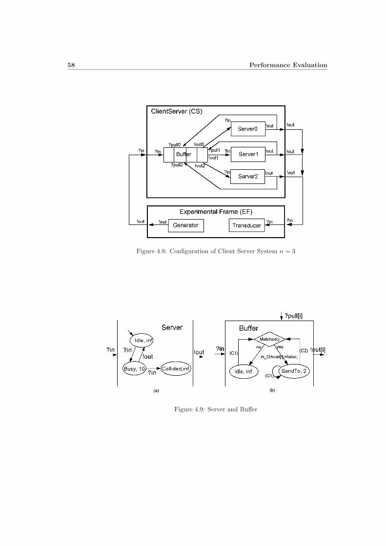
58 Performance Evaluation
Figure 4.8: Configuration of Client Server System n = 3
Figure 4.9: Server and Buffer
4.3 Client-Server System 59
public class Buffer: Atomic
{
public InputPort iin;
public List<InputPort> pull;
public List<OutputPort> oout;
private List<Job> m_Jobs; // FIFO Buffer
protected enum PHASE { Idle, SendTo, Ask };
protected PHASE m_phase;
protected List<bool> m_OAvail;//check availability of next resource
protected int m_Osize; // size of output
protected int m_send_index; // index to which it will send
protected double m_send_time;
The function C1 updates member data as a function of an input event x. Ifx comes through the input port in, C1 casts the value of x to Job and pushesit back to the buffer m_Jobs. Otherwise, x comes through one of pull ports.So C1 searches the server index i, checking the identity of pull[i] and theincoming event’s port, and updates m_OAvail[i]=true which marks the i-thserver as being available.
virtual protected void C1(PortValue x)
{
if(x.port == iin){ //receiving a client
if(x.value is Job) {
Job client = (Job)x.value;
if(client != null)
m_Jobs.Add(client);
}
else
throw new Exception("Invalid Input!");
}
else // receiving a pull signal
{
for(int i=0; i<m_Osize; i++) {
if(x.port == pull[i]) {
m_OAvail[i]= true; // server_i is available
break;
}
}
}
}

60 Performance Evaluation
The function Matched() first checks to see if there is a waiting job in m_Jobs
and then checks to see if there exists an available server from 0 to m_Osize-1. Ifa match is found, the function sets m_OAvail[i]=false, remembers the indexi at send_index, then returns true. Otherwise it returns false which meansno match.
private bool Matched()
{
if(m_Jobs.Count > 0){
for(int i=0; i < m_Osize; i++){// select server
if(m_OAvail[i] == true){// server i is available
m_OAvail[i]=false;//Mark server_i non-available
m_send_index = i; // remember i in m_send_index
return true;
}
}
return false;
}else
return false;
}
The function C2 creates an the output event and removes the first job fromm_Jobs when C2’s phase is SendTo.
virtual protected void C2(ref PortValue y)
{
if(m_phase == PHASE.SendTo){
Job job = m_Jobs[0];
y.Set(oout[m_send_index], job);
m_Jobs.RemoveAt(0);// remove the first client
}
}
The function init() of Buffer resets phase to Idle, assigns m_OAvial[i]=truefor all indices, and clears all jobs in m_Jobs.
public override void init()
{
m_phase = PHASE.Idle;
m_Jobs.Clear();
m_send_index = 0;
m_OAvail.Clear();
for (int i = 0; i < m_Osize; i++)
m_OAvail.Add(true); // add variable
}

4.3 Client-Server System 61
Buffer’s tau() returns ∞ for Idle and returns 2.0 for SendTo.
public override double tau()
{
if (m_phase == PHASE.Idle)
return double.MaxValue;
else
return m_send_time;
}
The input transition function delta_x of Buffer updates member data by call-ing C1(x) and then, if the phase of the server is Idle, checks the returning valueof Matched(). If the value is true, the phase of the server changes into SendTo.
public override bool delta_x(PortValue x)
{
C1(x);
if (m_phase == PHASE.Idle)
{
if (Matched())
{
m_phase = PHASE.SendTo;//
return true; // reschedule as active
}
}
return false;
}
When the server is ready to exit the state SendTo, it gets y by calling C2(y),if Matched() returns true, the phase stays at SendTo. Otherwise, the phasereturns to Idle.
public override void delta_y(ref PortValue y)
{
C2(ref y);
if (Matched())
m_phase = PHASE.SendTo;
else
m_phase = PHASE.Idle;
}
Recall that Buffer class contains the overriding Get_Statistics_s() andGetPerformance(), which were investigated in Section 4.2.3. For the codes ofBuffer::Get_s(), the reader should refer to Buffer.cs.
62 Performance Evaluation
4.3.3 Performance Analysis
The procedure for constructing the coupled model EF and CS is omitted herebecause it is quite straight forward and its schematics were shown in Figure 4.8.
All atomic models’ time units were set as TimeUnit.Sec. And Generator
used here was autonomous and it’s inter-generating job time was a randomnumber of the exponential pdf with mean 5; the time period at Busy of Serverwas constant 10; Buffer’s sending delay time was 2.
We will analyze change of performance indices by varying the number ofservers. The number of servers used in CS can be varied by passing different num-bers n with the following static function defined in Ex_ClientServer/Program_CS.cs.
static Coupled MakeTotalClientServerSystem(int n)
The simulation settings we use here are: the simulation ending time=10,000second; no display of continuously increasing te, the scale factor is maximum,in which the clock jumps to the next event time; and there is no display ofdiscrete event transitions. The following code shows the case where the numberof servers is 5.
static void Main(string[] args)
{
Coupled Sys = MakeTotalClientServerSystem(5) ;
Sys.PrintCouplings();
SRTEngine simEngine = new SRTEngine(Sys, 10000, null); //
simEngine.SetAnimationFlag(false);
simEngine.SetTimeScale(double.MaxValue); //
simEngine.Set_dtmode(SRTEngine.PrintStateMode.P_NONE, false);
simEngine.RunConsoleMenu();
}
Let’s change n sequentially from 1 to 5, and build the various system models,and try mrun 20 for each configuration. After completion of mrun 20, DEVS#summarizes the performance indices to the console. 2 Table 4.1 shows per-formance indices for each configuration and Figure 4.10s show the trend ofperformance changes as n changes.
Average Queue Length and Average System Time are drastically reduceduntil n reaches 3. Average Throughput increase up to 0.2 jobs/sec at n=3 andthen there is no increase at n=4 and 5. The reason why Throughput doesn’t
2The log file “devspp log.txt” collects also the same performance indices. But watch out
that the old devspp log.txt will be over written by the new one every time we execute DEVS#
again.
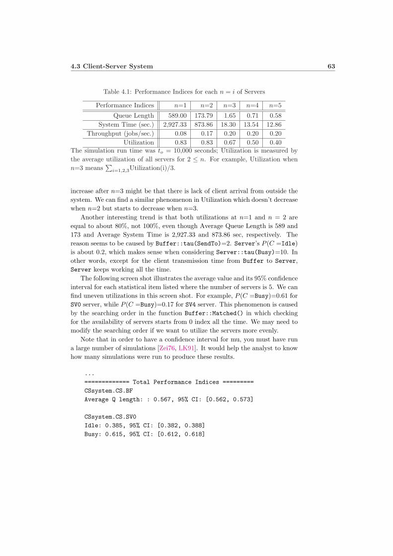
4.3 Client-Server System 63
Table 4.1: Performance Indices for each n = i of Servers
Performance Indices n=1 n=2 n=3 n=4 n=5
Queue Length 589.00 173.79 1.65 0.71 0.58System Time (sec.) 2,927.33 873.86 18.30 13.54 12.86
Throughput (jobs/sec.) 0.08 0.17 0.20 0.20 0.20Utilization 0.83 0.83 0.67 0.50 0.40
The simulation run time was to = 10,000 seconds; Utilization is measured bythe average utilization of all servers for 2 ≤ n. For example, Utilization whenn=3 means
∑i=1,2,3Utilization(i)/3.
increase after n=3 might be that there is lack of client arrival from outside thesystem. We can find a similar phenomenon in Utilization which doesn’t decreasewhen n=2 but starts to decrease when n=3.
Another interesting trend is that both utilizations at n=1 and n = 2 areequal to about 80%, not 100%, even though Average Queue Length is 589 and173 and Average System Time is 2,927.33 and 873.86 sec, respectively. Thereason seems to be caused by Buffer::tau(SendTo)=2. Server’s P (C =Idle)is about 0.2, which makes sense when considering Server::tau(Busy)=10. Inother words, except for the client transmission time from Buffer to Server,Server keeps working all the time.
The following screen shot illustrates the average value and its 95% confidenceinterval for each statistical item listed where the number of servers is 5. We canfind uneven utilizations in this screen shot. For example, P (C =Busy)=0.61 forSV0 server, while P (C =Busy)=0.17 for SV4 server. This phenomenon is causedby the searching order in the function Buffer::Matched() in which checkingfor the availability of servers starts from 0 index all the time. We may need tomodify the searching order if we want to utilize the servers more evenly.
Note that in order to have a confidence interval for mu, you must have runa large number of simulations [Zei76, LK91]. It would help the analyst to knowhow many simulations were run to produce these results.
...
============= Total Performance Indices =========
CSsystem.CS.BF
Average Q length: : 0.567, 95% CI: [0.562, 0.573]
CSsystem.CS.SV0
Idle: 0.385, 95% CI: [0.382, 0.388]
Busy: 0.615, 95% CI: [0.612, 0.618]
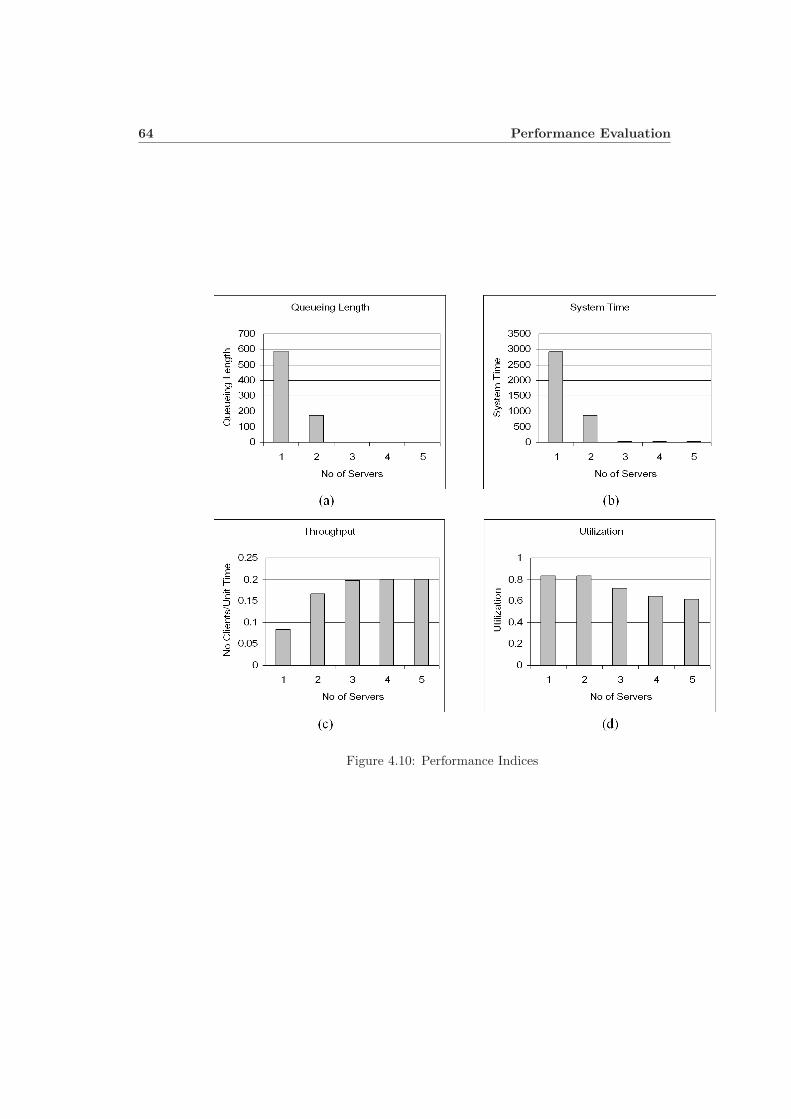
64 Performance Evaluation
Figure 4.10: Performance Indices

4.3 Client-Server System 65
CSsystem.CS.SV1
Idle: 0.471, 95% CI: [0.468, 0.474]
Busy: 0.529, 95% CI: [0.526, 0.532]
CSsystem.CS.SV2
Idle: 0.584, 95% CI: [0.581, 0.587]
Busy: 0.416, 95% CI: [0.413, 0.419]
CSsystem.CS.SV3
Idle: 0.713, 95% CI: [0.707, 0.718]
Busy: 0.287, 95% CI: [0.282, 0.293]
CSsystem.CS.SV4
Idle: 0.835, 95% CI: [0.830, 0.839]
Busy: 0.165, 95% CI: [0.161, 0.170]
CSsystem.EF.Trans
Average System Time of Job1 (Sec): 12.817, 95% CI: [12.791, 12.843]
# Job1 went through the system during 10000.00 Secs: 2011.500, 95% CI: [2000.585
, 2022.415]
Average Throughput of Job1 per Sec: 0.201, 95% CI: [0.200, 0.202]
========== Simulation Run Completed! ==========


Chapter 5
Appendix: Building
Projects using DEVS#
This appendix covers the directory structure of DEVS#, how to build the ex-ample projects provided in DEVS# library, and how to add new project.
5.1 Directory Structure of DEVS#
In DEVS# version 1.2.1, the root director of DEVS# is DEVSsharp in whichmany classes covered in Chapter 2 such as Named, Port, PortValue, Devs,Atomic, Coupled. However, the classes of random variables are containedin the sub-directory DEVSsharp\Util. DEVSsharp\Doc contais this documentin a PDF file and HTML files. DEVSsharp\Examples has example projectssuch as Ex_Timer, Ex_PingPong, Ex_VendingMaching, and Ex_ClientServer;DEVSsharp\ModelBase contains classes which can be used in several other projects
DEVSsharp
+-- Util
+-- Doc
+-- Examples
...
+-- ModelBase
...
+-- Verifiable
...
Figure 5.1: Directory Structure of DEVS#

68 Appendix: Building Projects using DEVS#
such as Generater, Transducer, Buffer, Server, and so on; DEVSsharp\Verifiablecontaining all classes which are used for verification that was not covered in thisdocument at all. For verification research, the author has a plan to write anotherdocument soon.
5.2 Building Simulation Examples in DEVS#
Modeling and simulation examples projects covered in Chapters 2, 3 and 4will be available DEVSsharp/Examples/Ex Projects. We can open each so-lution file whose file extension is sln in each project folder. For example,we can open DEVSsharp/Examples/Ex_ClientServer/Ex_ClientServer.sln.Each solution file will opens reference project(s) such as DEVSsharp (and ModelBase
for Ex_ClientServer) as well as the example project itself.In addition, if we open DEVSsharp/DEVSsharp.sln, Visual Studio 2005 will
open all examples of Timer, PingPong, ClientServer and VendingMachine aswell as DEVSsharp and ModelBase as shown in Solution Explorer window inFigure 5.2.
5.3 Adding Our Own Project
This section shows how to add new project which uses DEVS# library in astep-by-step procedure.
1. Create a new project. Select File->New->Project... menu. Then wecan see a dialog box as shown in Figure 5.3. We assume to create ConsoleApplication at DEVSsharp\Examples. The location we want to create newproject can be selected by [Browser...] button. The new project is titledas MyProject.
Then we can see the window screen of Visual Studio 2005 after creatingMyProject as shown in Figure 5.4.
2. Add DEVSshapr project. Since we need to use DEVSsharp library,we should add it by clicking right mouse button to ‘MyProject’ at So-lution Explorer and then select context menu through Add->Existing
Project... as shown in Figure 5.5. A file selection dialog will pop up,so we will select DEVSsharp\DEVSsharp.csproj that is the project file ofDEVSsharp.
3. Add DEVSsharp as a MyProject’s reference. Now we need to addDEVSshap project to MyProject as a reference. To do this, first left-button click MyProject at Solution Explorer and then select title menu
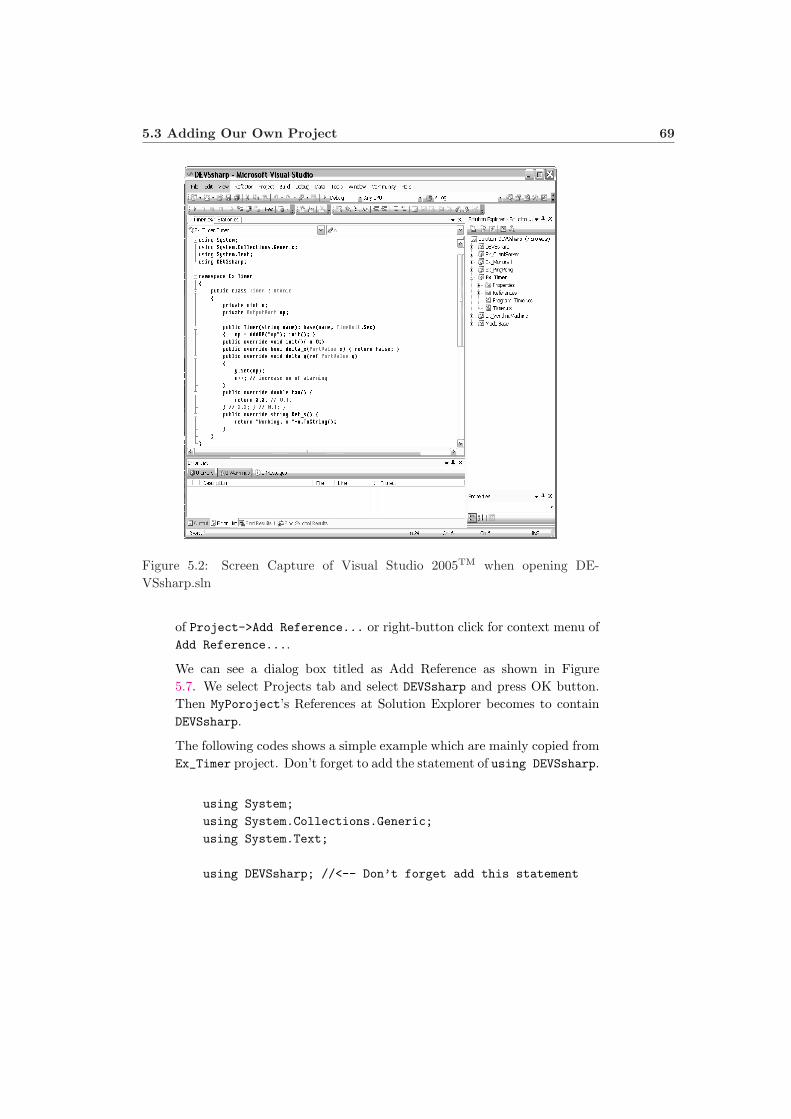
5.3 Adding Our Own Project 69
Figure 5.2: Screen Capture of Visual Studio 2005TM when opening DE-VSsharp.sln
of Project->Add Reference... or right-button click for context menu ofAdd Reference....
We can see a dialog box titled as Add Reference as shown in Figure5.7. We select Projects tab and select DEVSsharp and press OK button.Then MyPoroject’s References at Solution Explorer becomes to containDEVSsharp.
The following codes shows a simple example which are mainly copied fromEx_Timer project. Don’t forget to add the statement of using DEVSsharp.
using System;
using System.Collections.Generic;
using System.Text;
using DEVSsharp; //<-- Don’t forget add this statement

70 Appendix: Building Projects using DEVS#
Figure 5.3: New Project Dialog
namespace MyProject
{
public class Timer : Atomic
{
private OutputPort op;
public Timer(string name)
: base(name, TimeUnit.Sec)
{ op = AddOP("op"); init(); }
public override void init() { }
public override double tau() { return 3.3; }
public override bool delta_x(PortValue x) { return false; }
public override void delta_y(ref PortValue y) { y.Set(op); }
public override string Get_s() { return "Working"; }
}
class Program
{
static void Main(string[] args)
{
Timer timer = new Timer("STimer");
SRTEngine Engine = new SRTEngine(timer, 10000, null);

5.3 Adding Our Own Project 71
Figure 5.4: My Project
Engine.RunConsoleMenu();
}
}
}
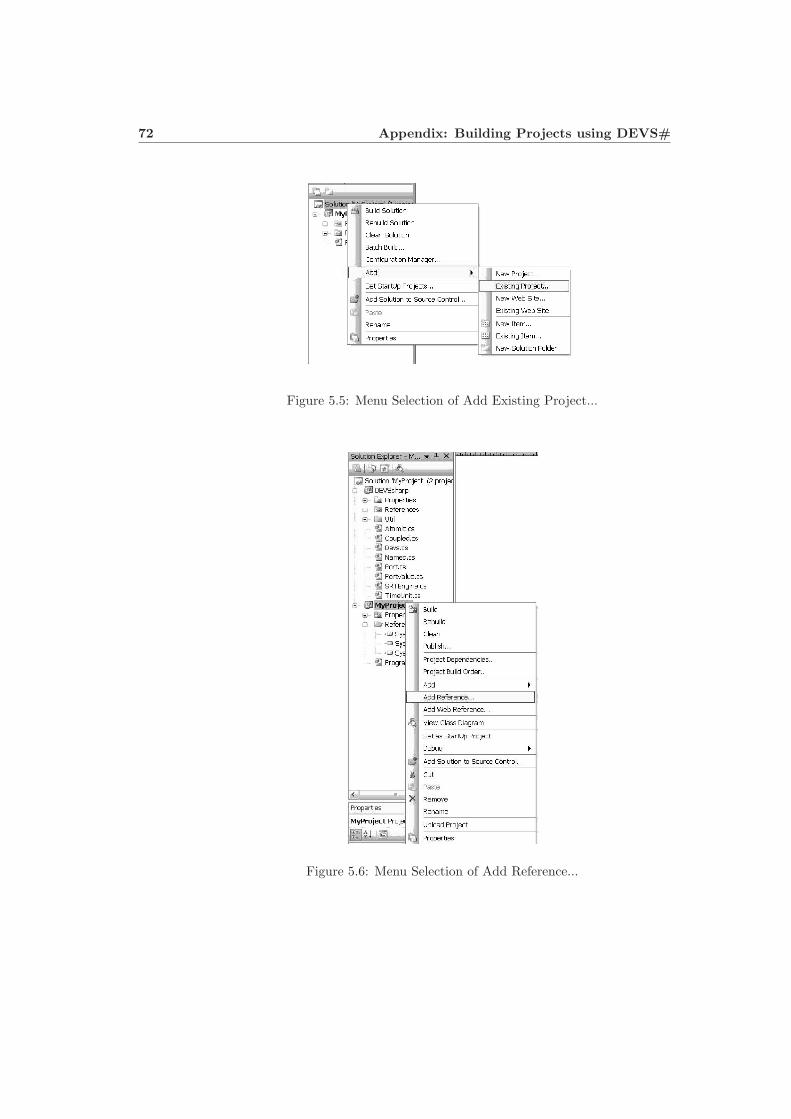
72 Appendix: Building Projects using DEVS#
Figure 5.5: Menu Selection of Add Existing Project...
Figure 5.6: Menu Selection of Add Reference...

5.3 Adding Our Own Project 73
Figure 5.7: Dialog of Add Reference


Bibliography
[Hwa07] Moon Ho Hwang. DEVS++: C++ Open Source Library of DEVSFormalism. http://odevspp.sourceforge.net/, first edition, Apr 2007.
[LK91] Averill M. Law and W. David Kelton. Simulation Modeling and Analy-sis. McGraw-Hill, New York, second edition, 1991.
[Zei76] Bernard P. Zeigler. Theory of Modelling and Simulation. Wiley Inter-science, New York, first edition, 1976.
[Zei87] Bernard P. Zeigler. Hierarchical, modular discrete-event modelling inan object-oriented environment. SIMULATION, 49(5):219–230, 1987.
[ZPK00] B. P. Zeigler, H. Praehofer, and T. G. Kim. Theory of Modellingand Simulation: Integrating Discrete Event and Continuous ComplexDynamic Systems. Academic Press, London, second edition, 2000.