General Physics Lab Department of PHYSICS YONSEI University

Lab Manual (Lite)

Momentum and Impulse Ver.20180328

Momentum and Impulse

Experiment 1:

Impulse-Momentum Theorem

(1) Set up equipment. (1-1) Install Universal Bracket at the left end of the track. (You will use this accessory in experiment 2.)

NOTICE This LITE version of manual includes only experimental procedures for easier reading on your smartphone. For more information and full instructions of the experiment, see the FULL version of manual.

Procedure

NOTE To mount any accessory to the track, ① Slide the tap and square nut of the accessory into the T-slot of the track. ② Tighten thumbscrew (clockwise) to secure it. To demount it, ① Loosen the thumbscrew (counterclockwise). ② Remove it with care.

When you loosen thumbscrew, NEVER try to completely unscrew it. (It won’t be reassembled again!)

(1-2) Install Photogate Bracket at the right end of the track. (You will use this accessory in experiment 2.)

(1-3) Mount the Motion Sensor. ① Mount the Motion Sensor on the left end of the track. ② Aim the sensor’s transducer at the cart (slightly up to avoid detecting the track-top). ③ Set the range switch to the short range ( ) setting.

(1-4) Install the Force Sensor. ① Install the End Stop at the right end of the track.

② Using FS thumbscrew, attach the Force sensor. ③ Screw the spring bumper into the Force Sensor.

(1-5) Connect the sensors to the interface.

(1-6) Adjust the inclination of the track. Use track feet to raise the Motion Sensor end of the track.

Do not raise the Motion Sensor end of the track too high. The faster the cart moves, the more likely that it may move to one side or the other during the collision. A smooth but slow collision is better than a fast, jerky one.

CAUTION Do not touch the mesh cover of the

Motion Sensor. Deformation of the cover could cause the sensor to fail.

CAUTION Do not tighten the bumper spring too hard. It could cause the Force sensor to fail. Treat it with care.

(2) Set up Capstone software. (2-1) Add [Motion Sensor] and [Force Sensor]. The interface automatically recognizes the Motion Sensor and the Force Sensor. (2-2) Configure the Force Sensor. Click the Force Sensor icon in the [Hardware Setup] panel

and then click the properties button (☼) in the lower right cor-ner. In the [Properties] window, Uncheck [Change Sign]. The sign of collected data of the Force sensor is initially positive for the pushing force.

(2-3) Adjust the sample rate of measurements. Select [1.00 kHz] for [High Resolution Force Sensor], and

[20.00 Hz] for [Motion Sensor] in the [Controls] palette.

(2-4) Add graph displays. ① Click and drag the [Graph] icon from the [Displays] palette into the workbook page. ② Click [Add new plot area … ] of the tool bar to add a 𝑥𝑥-axis synchronized graph. ③ Select [Time(s)] for the 𝑥𝑥-axis, and [Force(N)] and [Veloci-ty(m/s)] for each 𝑦𝑦-axis.

(3) Measure the mass of the Cart. 𝑚𝑚 = _________ (kg) (4) Mount the Cart on the Track. Place the cart in front of the Motion Sensor at least 15cm away. (The sensor cannot measure the distance closer than 15cm.) (5) Zero the Force Sensor. Press [ZERO] button on the sensor. You should zero the sensor prior to each data run.

(6) Begin recording data.

Click the [Record] button at the left end of the [Controls] palette to begin collecting data. The Motion Sensor starts clicking. If a target is in range, the target indicator flashes with each click. (7) Release the cart.

(8) Stop data collection. Wait until the cart stops after collision. When the cart stops, click [Stop].

(9) Analyze the data. ① Scaling and Panning graphs.

② Area under a curve Click [Select range(s) …] icon and then drag the data range

of interest.

Click [Display area …] icon to measure the area under the

curve.

NOTE The Motion Sensor uses an electrostatic transducer as

both a speaker and a microphone. For each sample, the transducer transmits a burst of 16 ultrasonic pluses. The ultrasonic pulses reflect off an object and return to the sensor. The sensor measures the time between the trig-ger rising edge and the echo rising edge. It uses this time and the speed of sound to calculate the distance to the object. You should remove objects that may interfere with the measurement. These include objects, and also your hand, between the sensor and target object, either direct-ly in front of the sensor or to the sides.

③ Data point Use [Show coordinates … ] icon to read off the data point.

④ Fit Function Because the Force Sensor (1kHz) and the Motion Sensor (20Hz) sample at the different rate, as you set in step (2-3), the resultant time intervals of measurements are different, as shown below.

The measured velocities are average velocities during each time interval so they could be quite different from the real instantaneous velocities in the region of sudden change. To find the velocity just before the collision and the velocity just after the collision, we need to find the fit function of the 𝑣𝑣-𝑡𝑡 graph. ① Using 𝐹𝐹-𝑡𝑡 graph, find the time just before the collision and the time just after the collision. ② Find the linear fits for the before-collision region and the after-collision region of 𝑣𝑣-𝑡𝑡 graph. ③ Calculate the instantaneous velocities by substituting ① into ②. Follow the steps below to find the linear fit for 𝑣𝑣-𝑡𝑡 graph. Click [Select range(s) …] icon and then drag the data range

of interest.

Click [Select curve fits … ] and select [Linear: mt+b] to find linear fit for selected data points.

(10) Verify impulse-momentum theorem. Find the experimental values of following equations by read-ing off the graphs, and verify impulse-momentum theorem.

𝒑𝒑��⃗ = 𝑚𝑚𝒗𝒗��⃗ (2)

𝑱𝑱��⃗ = � ∑ 𝑭𝑭��⃗ 𝑑𝑑𝑡𝑡𝑡𝑡2

𝑡𝑡1 (9)

𝑱𝑱��⃗ = 𝒑𝒑��⃗ 2 − 𝒑𝒑��⃗ 1 (7)

(11) Repeat measurement. ① Vary the collision speed by adjusting the inclination of the track or by adjusting the starting position of the cart. ② Change the bumper spring with different spring constant.

�𝐹𝐹𝑑𝑑𝑡𝑡 𝑝𝑝2 − 𝑝𝑝1

1

2

3

…

Experiment 2. Impulse

(1) Set up equipment. Follow the setup of experiment 1, and then, (1-1) Remove the Motion Sensor. (1-2) Install the Photogate. Attach the photogate on the bracket using a thumbscrew.

NOTE In this experiment, the Photogate works as an optical switch so that you can automatically start or stop data collection. The automatic measurement method is very helpful in easy analysis. However, if it looks complicated to use automatic meas-urement method, then you don’t have to use the Photo-gate. In this case, skip steps (1-2)~(1-4) and (2-2)~(2-5).

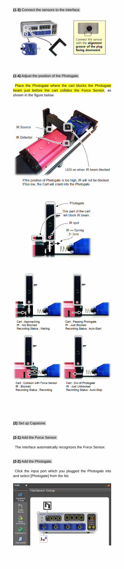
(1-3) Connect the sensors to the interface.

(1-4) Adjust the position of the Photogate. Place the Photogate where the cart blocks the Photogate beam just before the cart collides the Force Sensor, as shown in the figure below.

(2) Set up Capstone. (2-1) Add the Force Sensor. The interface automatically recognizes the Force Sensor. (2-2) Add the Photogate. Click the input port which you plugged the Photogate into

and select [Photogate] from the list.

(2-3) Create and configure a timer. Create a timer and configure automatic recording conditions.

① Click [Timer Setup] in the [Tools] palette, and then select [Pre-Configured Timer].

② Check [Photogate, Ch1].

③ Select [One Photogate (Single Flag)].

④ Check [State], which outputs the value of state of the

photogate. The photogate generates ‘1’ while it is blocked, and ‘0’ while open.

⑤ Skip steps ⑤ to ⑥ and finish the timer setup.

(2-4) Configure automatic recording conditions. ① Start Condition The cart approaches and blocks the IR of the photogate. The state value of the Photogate changes from ‘0’ to ‘1’. Start data collection

② Stop Condition The cart comes out of the Photogate after colliding with the

Force Sensor. (IR unblocked) The state value of the Photogate changes from ‘1’ to ‘0’. Stop data collection.

Click [Recording Conditions] in the [Controls] palette.

Select [Measurement Based] for [Condition Type] of [Start

Condition].

Set the parameters of [Start Condition] as below. [Condition Type] : Measurement Based [Data Source] : State() [Condition] : Is Above [Value] : 0.5

Set the parameters of [Stop Condition] as below.

[Condition Type] : Measurement Based [Data Source] : State() [Condition] : Is Below [Value] : 0.5

(2-5) Check the automatic recording configuration. You can see the [Record] button at the beginning.

If you click [Record], Capstone waits until the start condition

is achieved. ([Record] toggles to [Stop] and recording status display indicates [Waiting].) Even if the timer is ticking, no data is recorded.

If you block the photogate (start condition) using your finger,

data recording starts automatically. The recording status dis-play indicates [Recording].

If you open the photogate (stop condition), data recording

stops automatically. The status display indicates [Ready].

(2-6) Adjust the sample rate of measurements. Select [1.00 kHz] for [High Resolution Force Sensor].

(2-7) Create a graph display. Click and drag the [Graph] icon from the [Displays] palette

into the workbook page. Select [Time(s)] for the 𝑥𝑥-axis and [Force(N)] for the 𝑦𝑦-axis.

(3) Mount the cart on the track. Place the cart on the track at the starting position. Use the Universal Bracket so you can release the cart at the same position for all trials.

(4) Zero the Force Sensor. Press the [Zero] button on the sensor (5) Begin recording data. (6) Release the cart. Re-adjust the angle of the track, if required.

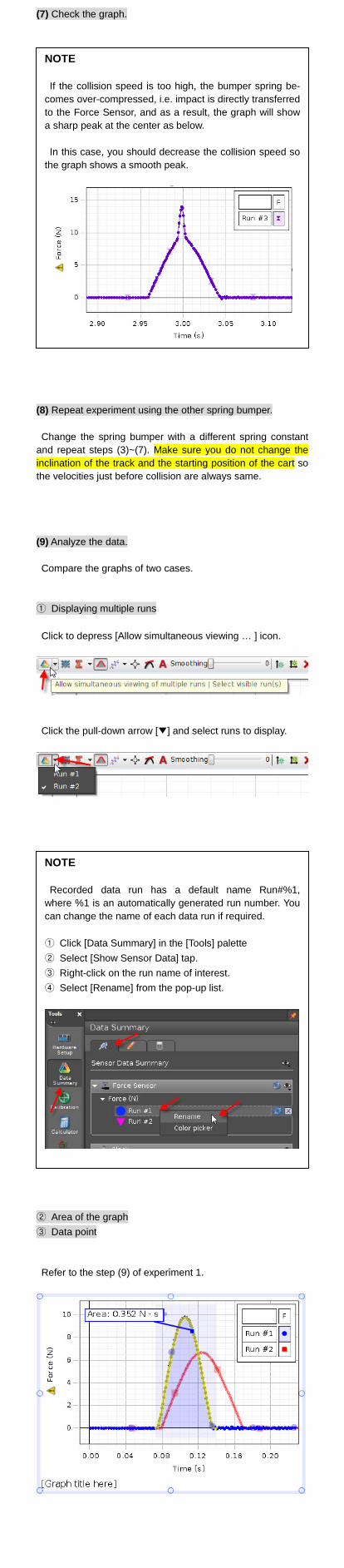
(7) Check the graph.

(8) Repeat experiment using the other spring bumper. Change the spring bumper with a different spring constant and repeat steps (3)~(7). Make sure you do not change the inclination of the track and the starting position of the cart so the velocities just before collision are always same. (9) Analyze the data. Compare the graphs of two cases.

① Displaying multiple runs Click to depress [Allow simultaneous viewing … ] icon.

Click the pull-down arrow [▼] and select runs to display.

② Area of the graph ③ Data point Refer to the step (9) of experiment 1.

NOTE If the collision speed is too high, the bumper spring be-comes over-compressed, i.e. impact is directly transferred to the Force Sensor, and as a result, the graph will show a sharp peak at the center as below. In this case, you should decrease the collision speed so the graph shows a smooth peak.

NOTE Recorded data run has a default name Run#%1,

where %1 is an automatically generated run number. You can change the name of each data run if required. ① Click [Data Summary] in the [Tools] palette ② Select [Show Sensor Data] tap. ③ Right-click on the run name of interest. ④ Select [Rename] from the pop-up list.

(10) Repeat measurement. Vary the collision speed by adjusting the inclination of the track or the starting position of the cart. Repeat steps (3)~(9). (11) Analyze your result. You do not measure the speed of the cart in this experiment. However, it is reasonable that the change in momentum is same for each run if you release the cart in the same position.

𝐽𝐽spring1 𝐽𝐽spring2

1st

2nd

3rd

Please put your equipment in order as shown below.

□ Delete your data files from your lab computer. □ Turn off the Computer and the Interface. □ Keep the Track Feet attached to the track. □ Assemble the Universal Bracket and Spring Bumper as shown below. □ Tighten all thumbscrews in position. □ Do not try to completely unscrew the thumbscrew and nut assembly of Track Feet, End Stops, and Brackets.

End of LAB Checklist