DC and AC Circuits - Yonseiphylab.yonsei.ac.kr/exp_ref/207_Circuit_ENG.pdf · DC and AC Circuits...

General Physics Lab (International Campus) Department of PHYSICS YONSEI University

Lab Manual

DC and AC CircuitsVer.20160901

Lab Office (Int’l Campus)

Room 301, Building 301 (Libertas Hall B), Yonsei University 85 Songdogwahak-ro, Yeonsu-gu, Incheon 21983, KOREA (☏ +82 32 749 3430) / 22

[International Campus Lab]

DC and AC Circuits

Determine the behavior of resistors, capacitors, and inductors in DC and AC circuits.

Symbols:

: Resistance (or resistor)

: Capacitance (or capacitor)

: Inductance (or inductor)

: Emf of the power source

: Instantaneous terminal voltage or potential difference

: Maximum terminal voltage (or voltage amplitude)

: Instantaneous current

: Maximum current (or current amplitude)

: Instantaneous charge on the capacitor

: Maximum charge on the capacitor

: Frequency

: Angular frequency, 2

: Reactance

: Impedance

1. Direct Current (DC) R-C Circuit

A circuit that has a resistor and a capacitor in series, as

shown in Fig.1, is called an R-C circuit. We idealize the bat-

tery to have a constant emf and zero internal resistance.

We begin with the capacitor initially uncharged (Fig.1a). At

some initial time 0 we close the switch, permitting cur-

rent around the loop to begin charging the capacitor (Fig.1b).

The potential differences across the capacitor and the

resistor are 0 and at 0

respectively. The initial current through the circuit is giv-

en by Ohm’s law: ⁄ ⁄ .

Fig. 1 Charging a capacitor. (a) Just before the switch is closed, the charge is zero. (b) When the switch closed (at 0), the current jumps from zero to / . As time passes, approaches and the

current approaches zero.

Objective

Theory

----------------------------- Reference --------------------------

Young & Freedman, University Physics (14th ed.), Pearson, 2016

26.4 R-C Circuit (p.886~890)

30.4 The R-L Circuit (p.1024~1028)

31.3 The L-R-C Series Circuit (p.1052~1056)

31.5 Resonance in AC Circuits (p.1060~1062)

-----------------------------------------------------------------------------


Lab Manual




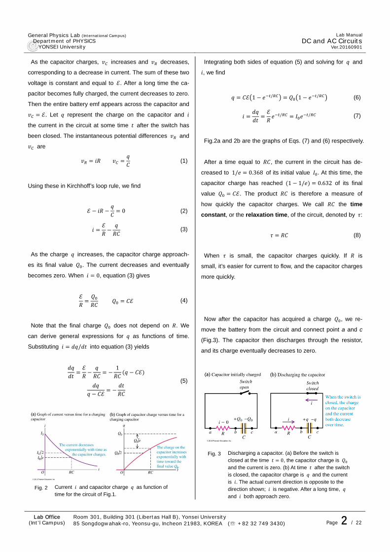
As the capacitor charges, increases and decreases,

corresponding to a decrease in current. The sum of these two

voltage is constant and equal to . After a long time the ca-

pacitor becomes fully charged, the current decreases to zero.

Then the entire battery emf appears across the capacitor and

. Let represent the charge on the capacitor and

the current in the circuit at some time after the switch has

been closed. The instantaneous potential differences and

are

(1)

Using these in Kirchhoff’s loop rule, we find

0 (2)

(3)

As the charge increases, the capacitor charge approach-

es its final value . The current decreases and eventually

becomes zero. When 0, equation (3) gives

(4)

Note that the final charge does not depend on . We

can derive general expressions for as functions of time.

Substituting / into equation (3) yields

1

(5)

Fig. 2 Current and capacitor charge as function of

time for the circuit of Fig.1.

Integrating both sides of equation (5) and solving for and

, we find

1 / 1 / (6)

/ / (7)

Fig.2a and 2b are the graphs of Eqs. (7) and (6) respectively.

After a time equal to , the current in the circuit has de-

creased to 1/ 0.368 of its initial value . At this time, the

capacitor charge has reached 1 1/ 0.632 of its final

value . The product is therefore a measure of

how quickly the capacitor charges. We call the time

constant, or the relaxation time, of the circuit, denoted by :

(8)

When is small, the capacitor charges quickly. If is

small, it’s easier for current to flow, and the capacitor charges

more quickly.

Now after the capacitor has acquired a charge , we re-

move the battery from the circuit and connect point a and c

(Fig.3). The capacitor then discharges through the resistor,

and its charge eventually decreases to zero.

Fig. 3 Discharging a capacitor. (a) Before the switch is closed at the time 0, the capacitor charge is and the current is zero. (b) At time after the switch is closed, the capacitor charge is and the current is . The actual current direction is opposite to the direction shown; is negative. After a long time, and both approach zero.


Lab Manual




In Fig.3 we make the same choice of the positive direction

for current as in Fig.1. Then Kirchhoff’s loop rule gives equa-

tion (3) but 0; that is,

(9)

The current is now negative; this is because positive charge

is leaving the left-hand capacitor plate in Fig.3b, so the

current is in the opposite to that shown in the figure.

At 0, when , the initial current is / . To

find , we rearrange and integrate equation (9), then we find

/ (10)

⁄ / (11)

We graph the current and the charge in Fig.4.

Substituting equations (6), (7), (10), (11) and ⁄

into equation (1) yields the terminal voltages across the ca-

pacitor and resistor as functions of time:

1 chargingcapacitor (12)

chargingcapacitor (13)

dischargingcapacitor (14)

dischargingcapacitor (15)

Fig. 4 Current and capacitor charge as function of time for the circuit of Fig.3.

2. Direct Current (DC) R-L Circuit

A circuit that includes both a resistor and an inductor, and

possibly a source of emf, is called an R-L circuit, as shown in

Fig.5. The inductor helps to prevent rapid changes in current.

Let be the current at some time after switch S is closed,

and let / be its rate of change at that time. The potential

differences and across the resistor

and the inductor at that time are

(16)

Using these in Kirchhoff’s loop rule, we find

0 (17)

1 ⁄ (18)

Fig. 5 An R-L circuit.

Fig. 6 (a) Graph of versus for growth of current in an

R-L circuit with and emf in series. The final current is ⁄ ; after one time constant , the current is

1 1/ of this value. (b) Graph of versus for decay of current in an R-L circuit. After one time constant , the current is 1/ of its initial value.


Lab Manual




As Fig.6a shows, the instantaneous current first rises rap-

idly, then increases more slowly and approaches the final

value / asymptotically. At a time equals to / , the

current has risen to 1 1/ 0.632 of its final value. The

quantity / is therefore a measure of how quickly the cur-

rent builds toward its final value; this quantity is called the

time constant for the circuit, denoted by :

(19)

Now suppose switch S in Fig.5 has been closed for a while

and the current has reached the value . We open S and

close S at the same time. Then the current through and

decays smoothly, as shown in Fig.6b. The Kirchhoff’s-rule

loop equation is obtained from equation (17) with 0, then

the current varies with time according to

⁄ (20)

The terminal voltages across the capacitor and resistor are

1 ⁄ 0 → (21)

⁄ 0 → (22)

⁄ → 0 (23)

⁄ → 0 (24)

3. Resistor in an AC Circuit

When a sinusoidal current cos flows through , as

shown in Fig.7a, the instantaneous voltage across is

cos (31)

The maximum voltage , the voltage amplitude, is the co-

efficient of the cosine function:

(32)

Hence we can also write

cos (33)

The current and voltage are both proportional to

cos , so the current is in phase with the voltage. Equation

(32) shows that the current and voltage amplitudes are relat-

ed in the same way as in a DC circuit. Fig.7b shows graphs

of and as functions of time. The vertical scales for cur-

rent and voltage are different, so the relative heights of the

two curves are not significant. The corresponding phasor

diagram is given in Fig.7c. Because and are in phase

and have the same frequency, the current and voltage phas-

ors rotate together; they are parallel at each instant. Their

projections on the horizontal axis represent the instantaneous

current and voltage, respectively.

Fig. 7 Resistance connected across an ac source.

Note

Equations (16)-(24) is valid only for an idealized inductor

which has negligible resistance. A real inductor generally

has resistance due to the resistance of a long fine

wire. Thus an inductor can be considered as L-RL combi-

nation in series. Then equations (21)~(24) become

⁄ 1 ⁄ 0 → (25)

⁄ ⁄ 0 → (26)

⁄ ⁄ → 0 (27)

⁄ ⁄ → 0 (28)


Lab Manual




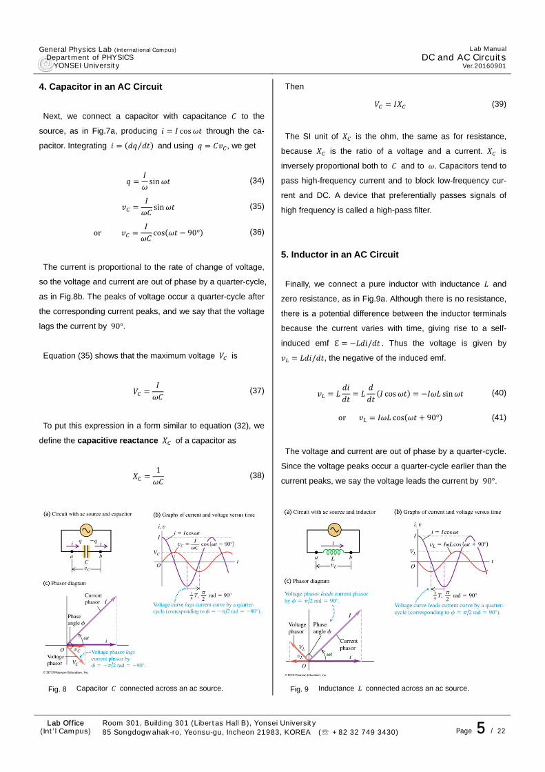
4. Capacitor in an AC Circuit

Next, we connect a capacitor with capacitance to the

source, as in Fig.7a, producing cos through the ca-

pacitor. Integrating ⁄ and using , we get

sin (34)

sin (35)

or cos 90° (36)

The current is proportional to the rate of change of voltage,

so the voltage and current are out of phase by a quarter-cycle,

as in Fig.8b. The peaks of voltage occur a quarter-cycle after

the corresponding current peaks, and we say that the voltage

lags the current by 90°.

Equation (35) shows that the maximum voltage is

(37)

To put this expression in a form similar to equation (32), we

define the capacitive reactance of a capacitor as

1

(38)

Fig. 8 Capacitor connected across an ac source.

Then

(39)

The SI unit of is the ohm, the same as for resistance,

because is the ratio of a voltage and a current. is

inversely proportional both to and to . Capacitors tend to

pass high-frequency current and to block low-frequency cur-

rent and DC. A device that preferentially passes signals of

high frequency is called a high-pass filter.

5. Inductor in an AC Circuit

Finally, we connect a pure inductor with inductance and

zero resistance, as in Fig.9a. Although there is no resistance,

there is a potential difference between the inductor terminals

because the current varies with time, giving rise to a self-

induced emf / . Thus the voltage is given by

/ , the negative of the induced emf.

cos sin (40)

or cos 90° (41)

The voltage and current are out of phase by a quarter-cycle.

Since the voltage peaks occur a quarter-cycle earlier than the

current peaks, we say the voltage leads the current by 90°.

Fig. 9 Inductance connected across an ac source.


Lab Manual




From equation (40), the amplitude is

(42)

We define the inductive reactance of an inductor as

(43)

Using , we can write equation (42) in a form similar to (32)

(44)

The inductive reactance is a description of the self-

induced emf that opposes any change in the current through

the inductor. Thus, according to equation (43), the inductive

reactance and self-induced emf increase with more rapid

variation in current (that is, increasing angular frequency )

and increasing inductance .

Since is proportional to frequency, a high-frequency

voltage applied to the inductor gives only a small current.

Inductors are used in some circuit applications to block high

frequencies while permitting lower frequencies or DC to pass

through. A circuit device that uses an inductor for this purpose

is called a low-pass filter.

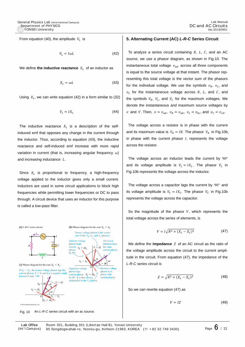
Fig. 10 An L-R-C series circuit with an ac source.

5. Alternating Current (AC) L-R-C Series Circuit

To analyze a series circuit containing , , , and an AC

source, we use a phasor diagram, as shown in Fig.10. The

instantaneous total voltage across all three components

is equal to the source voltage at that instant. The phasor rep-

resenting this total voltage is the vector sum of the phasors

for the individual voltage. We use the symbols , , and

for the instantaneous voltage across , , and , and

the symbols , , and for the maximum voltages. We

denote the instantaneous and maximum source voltages by

and . Then, , , , and .

The voltage across a resistor is in phase with the current

and its maximum value is . The phasor in Fig.10b,

in phase with the current phasor , represents the voltage

across the resistor.

The voltage across an inductor leads the current by 90°

and its voltage amplitude is . The phasor in

Fig.10b represents the voltage across the inductor.

The voltage across a capacitor lags the current by 90° and

its voltage amplitude is . The phasor in Fig.10b

represents the voltage across the capacitor.

So the magnitude of the phasor , which represents the

total voltage across the series of elements, is

(47)

We define the impedance of an AC circuit as the ratio of

the voltage amplitude across the circuit to the current ampli-

tude in the circuit. From equation (47), the impedance of the

L-R-C series circuit is

(48)

So we can rewrite equation (47) as

(49)


Lab Manual




Equation (49) has a form similar to , with impedance

in an AC circuit playing the role of resistance in a DC

circuit. Just as direct current tends to flow the path of least

resistance, so alternating current tends to follow the path of

lowest impedance.

We can see the meaning of impedance for a series circuit by

substituting and 1⁄ into equation (48).

1 (50)

Impedance is actually a function of , , , as well as of

the angular frequency . Hence for a given amplitude of

the source voltage applied to the circuit, the amplitude of

the resulting current will be different at different frequencies.

In the phasor diagram shown in Fig.10b, the angle be-

tween the voltage and current phasors is the phase angle of

the source voltage with respects to the current .

tan1⁄

(51)

If the current is cos , then the source voltage is

cos (52)

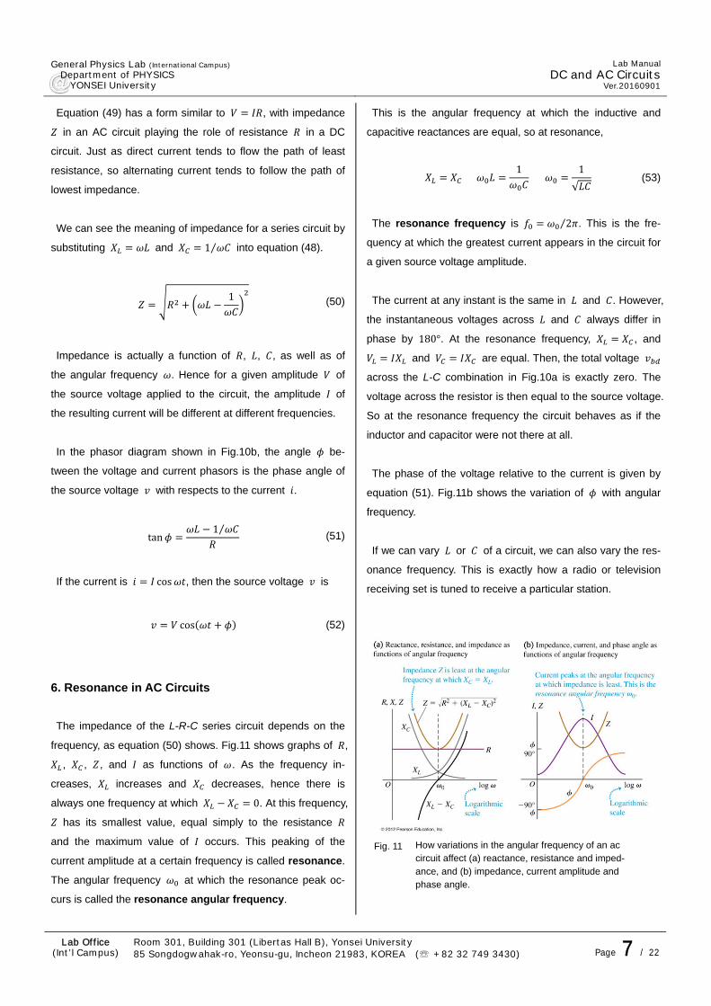
6. Resonance in AC Circuits

The impedance of the L-R-C series circuit depends on the

frequency, as equation (50) shows. Fig.11 shows graphs of ,

, , , and as functions of . As the frequency in-

creases, increases and decreases, hence there is

always one frequency at which 0. At this frequency,

has its smallest value, equal simply to the resistance

and the maximum value of occurs. This peaking of the

current amplitude at a certain frequency is called resonance.

The angular frequency at which the resonance peak oc-

curs is called the resonance angular frequency.

This is the angular frequency at which the inductive and

capacitive reactances are equal, so at resonance,

1

1

√ (53)

The resonance frequency is 2⁄ . This is the fre-

quency at which the greatest current appears in the circuit for

a given source voltage amplitude.

The current at any instant is the same in and . However,

the instantaneous voltages across and always differ in

phase by 180°. At the resonance frequency, , and

and are equal. Then, the total voltage

across the L-C combination in Fig.10a is exactly zero. The

voltage across the resistor is then equal to the source voltage.

So at the resonance frequency the circuit behaves as if the

inductor and capacitor were not there at all.

The phase of the voltage relative to the current is given by

equation (51). Fig.11b shows the variation of with angular

frequency.

If we can vary or of a circuit, we can also vary the res-

onance frequency. This is exactly how a radio or television

receiving set is tuned to receive a particular station.

Fig. 11 How variations in the angular frequency of an ac

circuit affect (a) reactance, resistance and imped-ance, and (b) impedance, current amplitude and phase angle.


Lab Manual




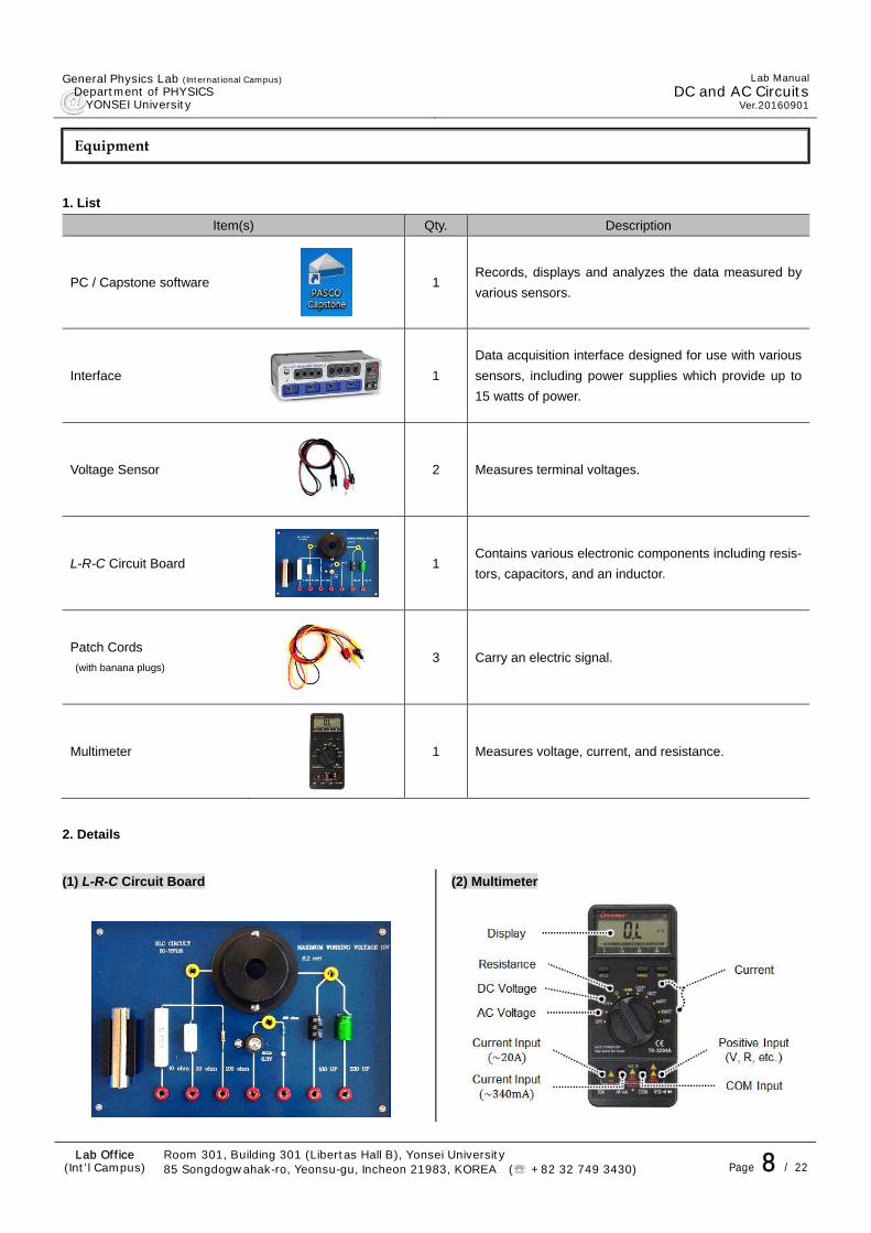
1. List

Item(s) Qty. Description

PC / Capstone software

1 Records, displays and analyzes the data measured by

various sensors.

Interface

1

Data acquisition interface designed for use with various

sensors, including power supplies which provide up to

15 watts of power.

Voltage Sensor

2 Measures terminal voltages.

L-R-C Circuit Board

1 Contains various electronic components including resis-

tors, capacitors, and an inductor.

Patch Cords

(with banana plugs)

3 Carry an electric signal.

Multimeter

1 Measures voltage, current, and resistance.

2. Details

(1) L-R-C Circuit Board

(2) Multimeter

Equipment


Lab Manual




Experiment 1. DC R-C Circuit

(1) Build an R-C circuit and connect the circuit to the interface.

① Connect the red banana plug patch cord from the red

[OUTPUT1] port of the interface to the bottom jack of the

330μF capacitor on the L-R-C circuit board.

② Connect the black patch cord from the black [OUTPUT1]

port of the interface to the bottom jack of 100Ω resistor.

③ Connect the yellow patch cord across the inductor.

④ Connect one voltage sensor to [Analog input A] on the

interface and attach the leads across the capacitor, making

sure the red cable of the voltage sensor is connected to the

bottom jack of the capacitor.

⑤ Connect the other voltage sensor to [Analog input B] on

the interface and attach the leads across the resistor, making

sure the black cable of the voltage sensor is connected to the

bottom jack of the resistor.

(2) Set up the PASCO Capstone program.

(2-1) Add sensors.

Click the ports which you plugged the sensors or patch

cords into and select [Voltage Sensor] or [Output Voltage

Current Sensor] from the list.

Procedure


Lab Manual




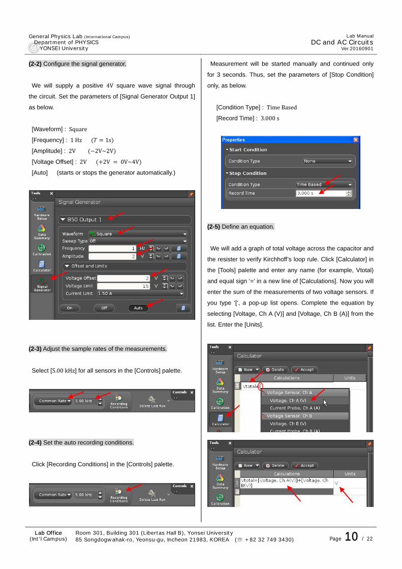
(2-2) Configure the signal generator.

We will supply a positive 4V square wave signal through

the circuit. Set the parameters of [Signal Generator Output 1]

as below.

[Waveform] : Square

[Frequency] : 1Hz 1s

[Amplitude] : 2V 2V~2V

[Voltage Offset] : 2V 2V 0V~4V

[Auto] (starts or stops the generator automatically.)

(2-3) Adjust the sample rates of the measurements.

Select [5.00kHz] for all sensors in the [Controls] palette.

(2-4) Set the auto recording conditions.

Click [Recording Conditions] in the [Controls] palette.

Measurement will be started manually and continued only

for 3 seconds. Thus, set the parameters of [Stop Condition]

only, as below.

[Condition Type] : TimeBased

[Record Time] : 3.000s

(2-5) Define an equation.

We will add a graph of total voltage across the capacitor and

the resister to verify Kirchhoff’s loop rule. Click [Calculator] in

the [Tools] palette and enter any name (for example, Vtotal)

and equal sign ‘=’ in a new line of [Calculations]. Now you will

enter the sum of the measurements of two voltage sensors. If

you type ‘[‘, a pop-up list opens. Complete the equation by

selecting [Voltage, Ch A (V)] and [Voltage, Ch B (A)] from the

list. Enter the [Units].


Lab Manual




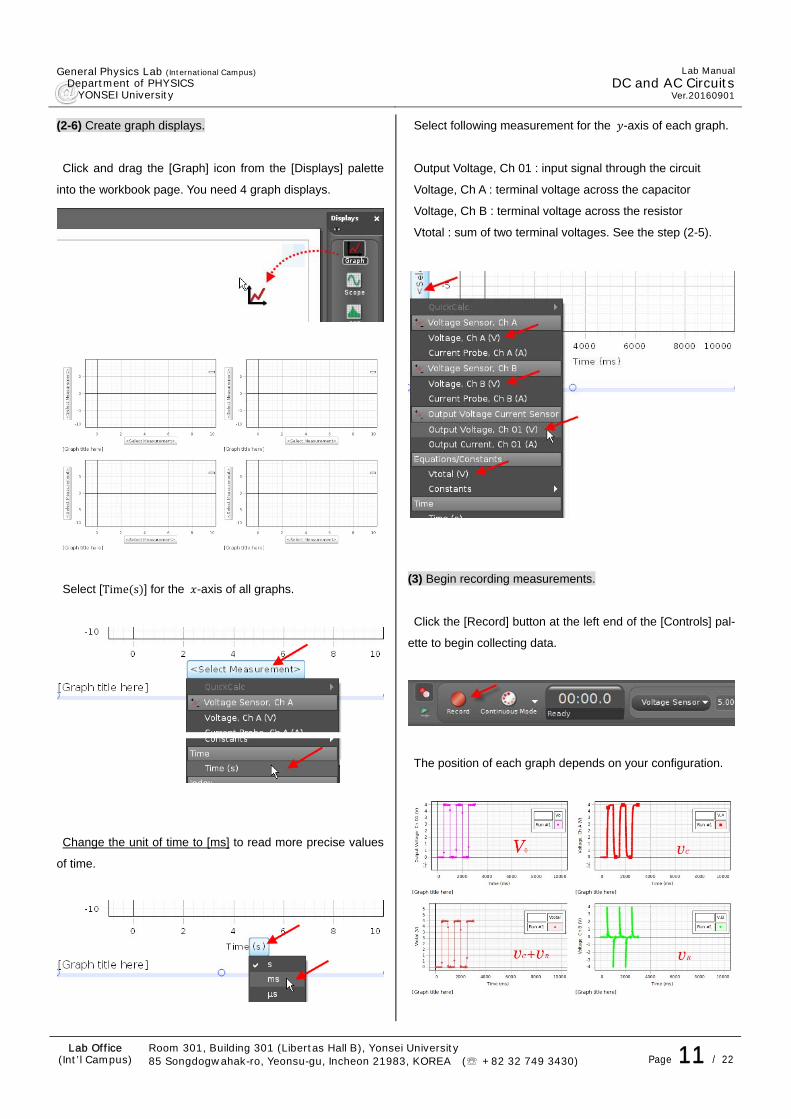
(2-6) Create graph displays.

Click and drag the [Graph] icon from the [Displays] palette

into the workbook page. You need 4 graph displays.

Select [Time s ] for the -axis of all graphs.

Change the unit of time to [ms] to read more precise values

of time.

Select following measurement for the -axis of each graph.

Output Voltage, Ch 01 : input signal through the circuit

Voltage, Ch A : terminal voltage across the capacitor

Voltage, Ch B : terminal voltage across the resistor

Vtotal : sum of two terminal voltages. See the step (2-5).

(3) Begin recording measurements.

Click the [Record] button at the left end of the [Controls] pal-

ette to begin collecting data.

The position of each graph depends on your configuration.


Lab Manual




(4) Analyze the graphs.

Adjust the scale of the graph. You can read off the coordi-

nates of the data using [Show coordinate…] icon.

(5) Analyze your results.

(5-1) Current through the R-C circuit

The graph of [Voltage, Ch B (A)], which is the terminal volt-

age across the resistor, represents through the

circuit, since is proportional to .

If you want to plot the graph of , you can use [Calculator].

Enter the equation ⁄ 100Ω in a new line of

[Calculations] and add one more graph of .

The graph of [Voltage, Ch A (A)], which is the terminal volt-

age / across the capacitor, represents on the

capacitor, since is proportional to . (You can also add

the graph of as explained above.)

Attach the graphs to the table below and compare them with

Fig.2 and Fig.4 of the [Theory].

Charging Discharging

or

or

(5-2) Kirchhoff’s loop rule

The graph of [Output Voltage, Ch 01] shows the emf

of the power source.

The graphs of [Voltage, Ch A (V)] and [Voltage, Ch B (A)]

show / and respectively.

Measure the voltages from the graphs for any 5 points of

time and verify Kirchhoff’s loop rule.

0 (2)

/ ⁄

The graph of [Vtotal] shows the sum of and . Com-

pare it with the graph of and verify the rule is always

valid.


Lab Manual




(5-3) Capacitance of the capacitor

Equations (12) and (14) represent the terminal voltage of the

charging or discharging capacitor.

1 / chargingcapacitor (12)

/ dischargingcapacitor (14)

If you know , you can find using your result and the

equations above.

After a time equal to , the capacitor charge has risen to

1 1/ 0.632 of its final value, i.e. the terminal voltage

across the capacitor reaches 63.2% of the input voltage

. Find the time from the graph, and then calculate the

capacitance of the capacitor using following equations.

1 1/ 1 / or ⁄

Similarly, find the time at which the charge of discharg-

ing capacitor reaches 1/ 36.8% of the initial value. Calcu-

late using following equations.

1/ / or ⁄ .

charging discharging

result

average

marked

(6) Repeat the experiment with 100μF capacitor.

Using 100μF and 100Ω, repeat the steps (3)-(5).

(7) Compare the results.

Compare the graphs of the terminal voltages across 330μF

and 100μF capacitors.

[…viewing of multiple runs | Select …] or [▼] activates view-

ing multiple runs together.

Attach the graphs and answer the following questions.

Q

Describe the difference of the graphs.

What is the physical meaning of the difference?

Explain your result using the time constant

A

Note

Most resistors and capacitors have a tolerance rating

expressed as a percentage. The tolerance value is the

extent to which the actual value is allowed to vary from its

nominal value. The tolerance is usually indicated by col-

ored stripes or codes on the surface. The most common

tolerance variation is 1~10% for resistors and 5~20% for

capacitors.


Lab Manual




Experiment 2. DC R-L Circuits

(1) Build an R-L circuit and connect the circuit to the interface.

① Connect the red banana plug patch cord from the red

[OUTPUT1] port of the interface to the right jack of the

8.2mH inductor on the L-R-C circuit board.

② Connect the black patch cord from the black [OUTPUT1]

port of the interface to the bottom jack of 100Ω resistor.

③ Connect one voltage sensor to [Analog input A] on the

interface and attach the leads across the inductor, making

sure the red cable of the voltage sensor is connected to the

right jack of the inductor.

④ Connect the other voltage sensor to [Analog input B] on

the interface and attach the leads across the resistor, making

sure the black cable of the voltage sensor is connected to the

bottom jack of the resistor.

⑤ Insert the iron core inside the inductor.


Follow the steps of the previous experiment, EXCEPT NEXT.

(Before you modify configuration, you should save your data

of the R-C experiment with a different file name!)

(2-1) Configure the signal generator.

[Waveform] : Square

[Frequency] : 0.01s


[Voltage Offset] : 2V 2V 0V~4V

[Auto] (starts or stops the generator automatically.)

If the input voltage alternates before the terminal voltage

approaches a certain value, set [Frequency] at 50Hz.

(2-2) Adjust the sample rates of the measurements.

Select [ . ] for all sensors in the [Controls] palette.

If you set the sample rates too high, the computer system

may stop with an error message. If you have any problem

proceeding the experiment with 50kHz, decrease the sample

rates. However, remember that too low rate precludes the

accurate analysis of the result.


Lab Manual




(2-3) Set the auto recording conditions.

Click [Recording Conditions] in the [Controls] palette.

The measurements will be started manually and continued

for only 0.03 seconds. Set the parameters of [Stop Condition]

as below. (The computer system may stop if the measuring

time is too long.)

[Condition Type] : TimeBased

[Record Time] : .

(3) Begin recording measurements.

The position of each graph depends on your configuration.

(If the input voltage alternates before the terminal voltage

approaches a certain value, set [Frequency] at 50Hz. See

step (2-1))

(4) Analyze the graphs.


(5-1) [Optional] Internal resistance of an inductor

The graphs show that the terminal voltages across the in-

ductor and the resistor do not approach the values as we

predicted.

These result from the internal resistance of the inductor.

For more accurate observations, we should consider .

Measure the asymptotic values of and and calculate

using ⁄ ⁄ .

Note

The terminal voltage across the inductor theoretically

decreases from the input voltage, 4V , however, your

graph will probably not, since the interface cannot detect

the sudden change of voltage.


Lab Manual




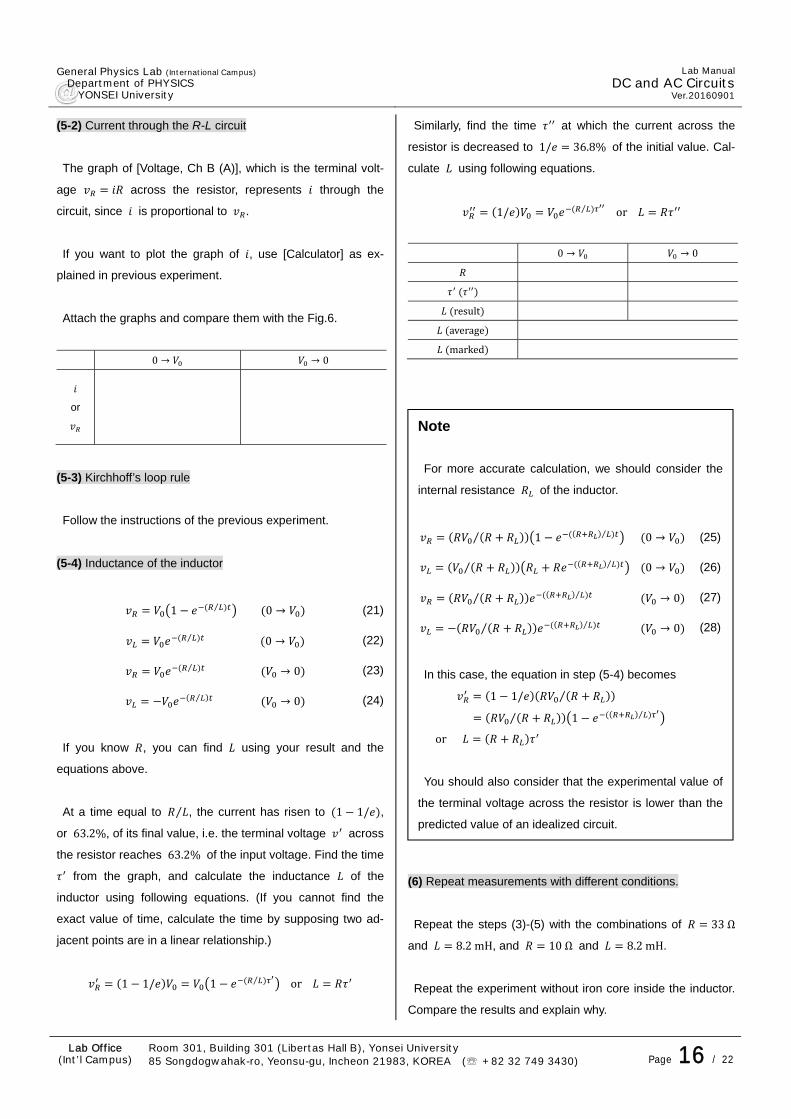
(5-2) Current through the R-L circuit

The graph of [Voltage, Ch B (A)], which is the terminal volt-

age across the resistor, represents through the

circuit, since is proportional to .

If you want to plot the graph of , use [Calculator] as ex-

plained in previous experiment.

Attach the graphs and compare them with the Fig.6.

0 → → 0

or

(5-3) Kirchhoff’s loop rule

Follow the instructions of the previous experiment.

(5-4) Inductance of the inductor

1 ⁄ 0 → (21)

⁄ 0 → (22)

⁄ → 0 (23)

⁄ → 0 (24)

If you know , you can find using your result and the

equations above.

At a time equal to ⁄ , the current has risen to 1 1/ ,

or 63.2%, of its final value, i.e. the terminal voltage across

the resistor reaches 63.2% of the input voltage. Find the time

from the graph, and calculate the inductance of the

inductor using following equations. (If you cannot find the

exact value of time, calculate the time by supposing two ad-

jacent points are in a linear relationship.)

1 1/ 1 ⁄ or

Similarly, find the time at which the current across the

resistor is decreased to 1/ 36.8% of the initial value. Cal-

culate using following equations.

1/ ⁄ or

0 → → 0

result

average

marked

(6) Repeat measurements with different conditions.

Repeat the steps (3)-(5) with the combinations of 33Ω

and 8.2mH, and 10Ω and 8.2mH.

Repeat the experiment without iron core inside the inductor.

Compare the results and explain why.

1 1/ ⁄

⁄ 1 ⁄

or

Note

For more accurate calculation, we should consider the

internal resistance of the inductor.

⁄ 1 ⁄ 0 → (25)

⁄ ⁄ 0 → (26)

⁄ ⁄ → 0 (27)

⁄ ⁄ → 0 (28)

In this case, the equation in step (5-4) becomes

You should also consider that the experimental value of

the terminal voltage across the resistor is lower than the

predicted value of an idealized circuit.


Lab Manual




Experiment 3. Resistor in an AC Circuit

(1) Connect 10Ω to the interface signal output.


(2-1) Add an [Output Voltage Current Sensor].

(2-2) Configure [Signal generator].

[Waveform] : Sine

[Frequency] : 100Hz 0.01s


[Auto]

(2-3) Create a scope display.

Click and drag the [Scope] icon from the [Displays] palette

into the workbook page.

(2-4) Add an independent -axis on the right of the graph.

(2-5) Define the axes.

-axis: Time(s)

-axis(left): Output Voltage (V)

-axis(right): Output Current (A)


Lab Manual




(2-6) Select [Fast Monitor Mode] in the controls palette.

[Fast Monitor Mode] displays data without recording. Check

that [Recode] button is changed to [Monitor] button.

(3) Start monitoring data.

(3-1) Click [Monitor] in the controls palette.

(3-2) Click [Activate … trigger] in the toolbar to horizontally

align repetitions of the signal.

Color in legend matches plot color.


Measure the phase difference between cos

and cos . Compare your result with Fig.7 in [Theory].

Experiment 4. Capacitor in an AC Circuit

Connect 100μF to the interface signal output.

[Waveform] : Sine

[Frequency] : 100Hz 0.01s





Lab Manual




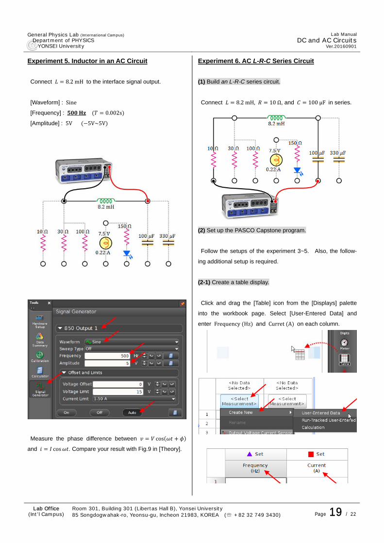
Experiment 5. Inductor in an AC Circuit

Connect 8.2mH to the interface signal output.

[Waveform] : Sine

[Frequency] : 0.002s




Experiment 6. AC L-R-C Series Circuit

(1) Build an L-R-C series circuit.

Connect 8.2mH, 10Ω, and 100μF in series.


Follow the setups of the experiment 3~5. Also, the follow-

ing additional setup is required.

(2-1) Create a table display.

Click and drag the [Table] icon from the [Displays] palette

into the workbook page. Select [User-Entered Data] and

enter Frequency Hz and Curret A on each column.


Lab Manual




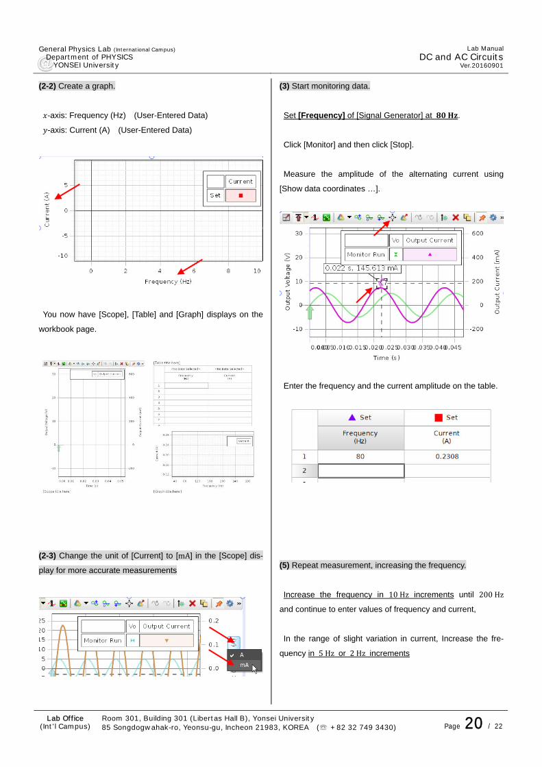
(2-2) Create a graph.

-axis: Frequency (Hz) (User-Entered Data)

-axis: Current (A) (User-Entered Data)

You now have [Scope], [Table] and [Graph] displays on the

workbook page.

(2-3) Change the unit of [Current] to [mA] in the [Scope] dis-

play for more accurate measurements

(3) Start monitoring data.

Set [Frequency] of [Signal Generator] at .

Click [Monitor] and then click [Stop].

Measure the amplitude of the alternating current using

[Show data coordinates …].

Enter the frequency and the current amplitude on the table.

(5) Repeat measurement, increasing the frequency.

Increase the frequency in 10Hz increments until 200Hz

and continue to enter values of frequency and current,

In the range of slight variation in current, Increase the fre-

quency in 5Hz or 2Hz increments


Lab Manual




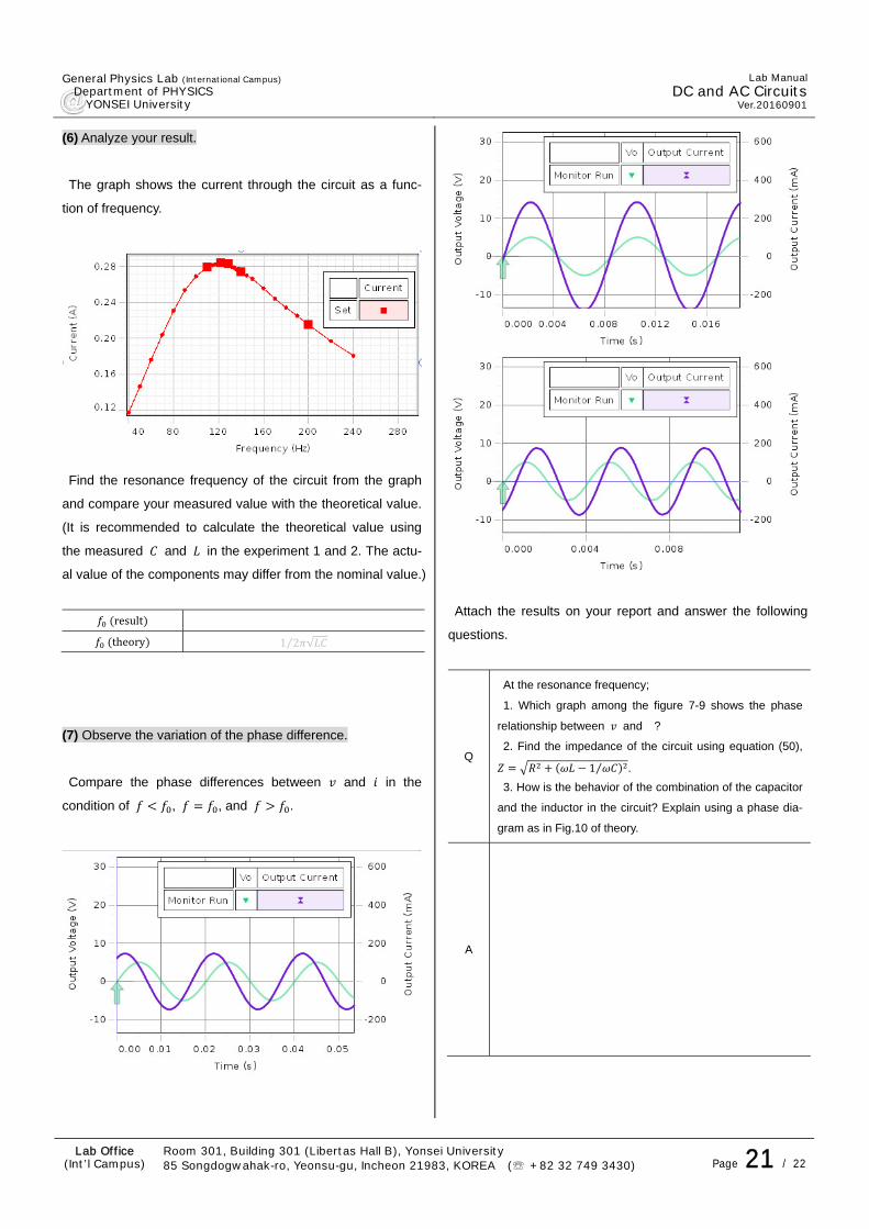
(6) Analyze your result.

The graph shows the current through the circuit as a func-

tion of frequency.

Find the resonance frequency of the circuit from the graph

and compare your measured value with the theoretical value.

(It is recommended to calculate the theoretical value using

the measured and in the experiment 1 and 2. The actu-

al value of the components may differ from the nominal value.)

result

theory 1 2 √⁄

(7) Observe the variation of the phase difference.

Compare the phase differences between and in the

condition of , , and .

Attach the results on your report and answer the following

questions.

Q

At the resonance frequency;

1. Which graph among the figure 7-9 shows the phase

relationship between and ?

2. Find the impedance of the circuit using equation (50),

1⁄ .

3. How is the behavior of the combination of the capacitor

and the inductor in the circuit? Explain using a phase dia-

gram as in Fig.10 of theory.

A


Lab Manual




Your TA will inform you of the guidelines for writing the laboratory report during the lecture.

Please put your equipment in order as shown below.

□ Delete your data files and empty the trash can from the lab computer.

□ Turn off the Computer and the Interface.

□ Return the Iron Core of the inductor to its storage location on the L-R-C circuit board.

□ Handle the L-R-C Circuit Board with care. The plastic case is fragile.

□ Turn off the Multimeter.

Result & Discussion

End of Lab Checklist

DC and AC Circuits - Yonseiphylab.yonsei.ac.kr/exp_ref/207_Circuit_ENG.pdf · DC and AC Circuits...

Documents

Transcript of DC and AC Circuits - Yonseiphylab.yonsei.ac.kr/exp_ref/207_Circuit_ENG.pdf · DC and AC Circuits...