Spot Image, 1999, with shellfish leases and polders represented (GIS in development)

MODELLING THE GROWTH OF MYTILUS EDULIS (L.) BY COUPLING A DYNAMIC ENERGY BUDGET MODEL WITH SATELLITE DERIVED ENVIRONMENTAL DATA

Yoann Thomas, Joseph Mazurié, StéphanePouvreau, Cédric Bacher, Francis Gohin,

Caroline Struski, Patrick Le Mao

Ifremer Brest, La Trinité/mer, Saint-Malo

Ackowledgments to the SRC-BN (Section Régionale de la Conchyliculture de Bretagne Nord)

fot its support

Sedimentary enclave of 500 km2

intertidal zone of 240 km2

Bed communities dominated by suspension feeders, both natural, cultivated and invasive

Mont Saint-Michel bay

The site and shellfish farming

Yoann Thomas

Oyster O. edulisStock 3000 tonsProduction 1500 tons

Oyster C. gigasStock 8000 tonsProduction 5000 tons

Mussel M. edulisStock 10-12000 tonsProduction 10-12000 tons (~320,000 poles)

2003->2006 :spatial reorganisation of shellfish leases

1- 150 000 mussel poles ->Easward (more productive ?)

1

2- 150 ha of oyster leases -> Eastward (less muddy)

2

=> Questions about Carrying Capacity of the Bay ?

Objective of the study

develop a growth model of Mytilus edulis based on Dynamic Energy Budget Theory (Kooijman, 2000)

Within the framework of

Assess the variability of mussel growth with respect to spatial and temporal variability of environmental parameters

Use Satellite data as forcing variables (spatially available)

Summary

1. Growth data (sampling strategy, variables)

2. Satellite data(Sources, data, validation, images…)

3. Model implementation(assumptions, calibration, application at two scales)

4. Discussion-Conclusion

I- Growth data acquisitionSAMPLING 3x5 Poles from 5 zones (A, B, C, D, E) harvested every 2 month, (april to dec. 2004) and then sub-sampled for measurements

A B

C

D

E

extension

1 km

Mussel growth april to oct 2004

0.0

2.0

4.0

6.0

8.0

10.0

12.0

1/6

1/8

1/10

1/12

31/1 1/4

1/6

1/8

1/10

1/12

31/1

who

le w

eigh

t per

mus

sell

(g) E

D

B

C

A

=> Growth exhibits a positive gradientbetween ancient area (A, B, C)

and new area (D, E)(mainly acquired during the 1st year 2003)

GROWTH VARIABLES Whole, shell, meat weights…(2nd year of growth)

1st year 2003

2nd year2004

II- Satellite Imagery : (1) Sources

ftp://ftp.ifremer.fr/ifremer/cersat/products/gridded/ocean-color/

Data (Geotiff, NetCdf)

http://www.ifremer.fr/nausicaa/marcoast/index.htm /roses/index.htm

/gascogne/index.htm/medit/index.htm

Maps(on simple registration)

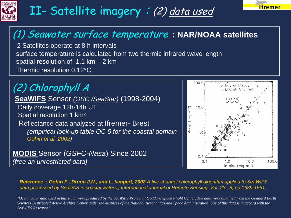
II- Satellite imagery : (2) data used

(1) Seawater surface temperature : NAR/NOAA satellites 2 Satellites operate at 8 h intervals surface temperature is calculated from two thermic infrared wave length spatial resolution of 1.1 km – 2 kmThermic resolution 0.12°C:

(2) Chlorophyll ASeaWIFS Sensor (OSC /SeaStar) (1998-2004) Daily coverage 12h-14h UT Spatial resolution 1 km²Reflectance data analyzed at Ifremer- Brest

(empirical look-up table OC 5 for the coastal domain Gohin et al. 2002)

MODIS Sensor (GSFC-Nasa) Since 2002 (free an unrestricted data)

"Ocean color data used in this study were produced by the SeaWiFS Project at Goddard Space Flight Center. The data were obtained from the Goddard Earth Sciences Distributed Active Archive Center under the auspices of the National Aeronautics and Space Administration. Use of this data is in accord with the SeaWiFS Research"

Reference : Gohin F., Druon J.N., and L. lampert, 2002 A five channel chlorophyll algorithm applied to SeaWiFSdata processed by SeaDAS in coastal waters,, International Journal of Remote Sensing, Vol. 23 , 8, pp 1639-1661,

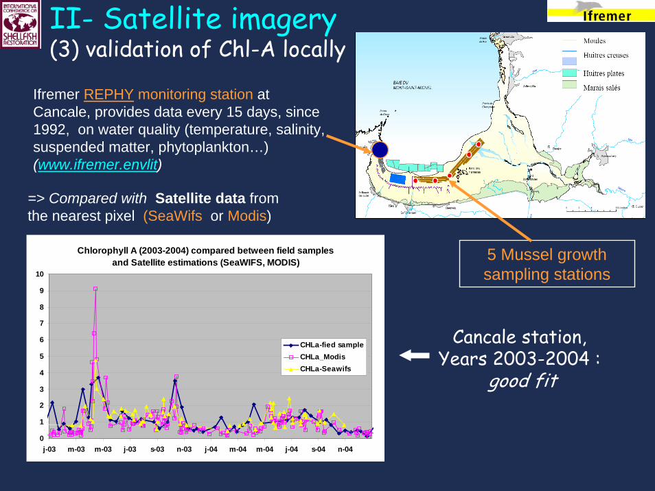
II- Satellite imagery(3) validation of Chl-A locally

Cancale station, Years 2003-2004 :

good fit

Chlorophyll A (2003-2004) compared between field samples and Satellite estimations (SeaWIFS, MODIS)

0

1

2

3

4

5

6

7

8

9

10

j-03 m-03 m-03 j-03 s-03 n-03 j-04 m-04 m-04 j-04 s-04 n-04

CHLa-fied sampleCHLa_ModisCHLa-Seawifs

Ifremer REPHY monitoring station at Cancale, provides data every 15 days, since1992, on water quality (temperature, salinity, suspended matter, phytoplankton…) (www.ifremer.envlit)

5 Mussel growth sampling stations

=> Compared with Satellite data from the nearest pixel (SeaWifs or Modis)

Modis OC5 IFR Choro 02/08/2003

Modis OC5 IFR Choro 04/10/2003

Modis OC5 IFR Choro 24/01/2003

Modis OC5 IFR Choro 06/05/2003

II-Satellite imagery : (3) Typical Chl-A images, per season

III Growth model (1) experimental sources for main assumptions

Food source = phytoplankton

(Chl-a)

Isotopic markers : Mussels food : 80 % ocean POM (mainly Phytoplankton)

Riera (2007)

Food ingestion = Maximum ingestion rate : experimental (Pouvreau, Ifremer)

Reproduction period and

effort

From histology (Donval, Brest Un.) => Spawnings in march-april

0.40

0.50

0.60

0.70

0.80

INIT-2ans PONDU-2ans

TDW

(g)

perte = 34%

Experimental spawnings at lab =>34% weight loss

0123456789

101112

j j a s o n d j f m a m j j a s o n d j

Poid

s en

tier (

g)

HoLesimulé-Hermelles

Growth data

The DEB Modeldetailed in next presentations

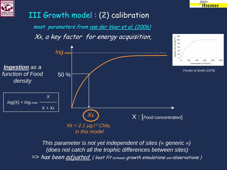
III Growth model : (2) calibration

Ingestion as a function of Food

density

Ing.max

50 %

Xk X : [Food concentration]

This parameter is not yet independent of sites (« generic »)(does not catch all the trophic differences between sites)

=> has been adjusted ( best fit between growth simulations and observations )

Xk = 2.1 µg.l-1 Chla, in this model

0

20

40

60

80

100

120

0 200 400 600 800 1000

Concentration (10-3cell.ml-1)

Inge

stio

n ra

te (1

0-6ce

lls.h

-1)

Ing(X) = Ing.max

X + Xk

Forster & Smith (1975)

X

Xk, a key factor for energy acquisition,most parameters from van der Veer et al. (2006)

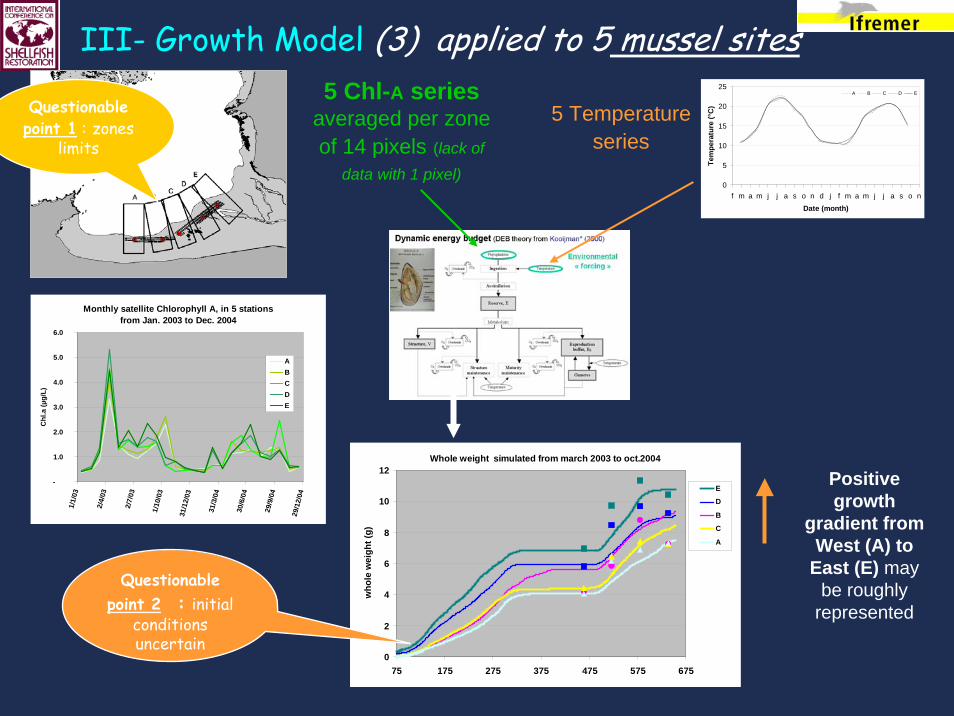
III- Growth Model (3) applied to 5 mussel sites

0

5

10

15

20

25

f m a m j j a s o n d j f m a m j j a s o n

Date (month)

Tem

pera

ture

(°C

)

A B C D E

5 Temperature series

5 Chl-A series averaged per zone of 14 pixels (lack of

data with 1 pixel)

Monthly satellite Chlorophyll A, in 5 stations from Jan. 2003 to Dec. 2004

-

1.0

2.0

3.0

4.0

5.0

6.0

1/1/

03

2/4/

03

2/7/

03

1/10

/03

31/1

2/03

31/3

/04

30/6

/04

29/9

/04

29/1

2/04

Chl

.a (µ

g/L)

ABCDE

Whole weight simulated from march 2003 to oct.2004

0

2

4

6

8

10

12

75 175 275 375 475 575 675

who

le w

eigh

t (g)

E

D

B

C

A

Positive growth

gradient from West (A) to

East (E) may be roughly

represented

Questionable point 1 : zones

limits

Questionablepoint 2 : initial

conditions uncertain

III Growth Model : (4) applied at bay scale

378 pixels of Chla monthly

averages

378 pixels of Temperature

monthly averages

Simulated Weight at harvest

Final whole weight as a function of mean Chl- A

y = 9.4x - 3.6R2 = 0.85

0

5

10

15

20

25

0.00 0.50 1.00 1.50 2.00 2.50 3.00

mean Chl-A over growth period

Fina

l Who

le W

eigh

t (g)

Mean Chl-A => Weight at harvest (after 18 month growth)

Conclusion : Main Results

1- Temperature, Chl-A (and suspended matter) appear to be fairly estimated by existing treatments of satellite seawater reflectance data.

2- Ecophysiological models (specially of DEB type) establish the relationship between these environmental parameters and Growth of various species

=> Forcing of ecophysiological Growth Models with satellite environmental data broadens their field to application (habitat suitability, aquaculture potential, GIS…)

Discussion : limits of the study, perspectives

1. Limits of the growth data useduncontrolled initial conditions, sampling variations…=> (use of experimental standard mesh bags…)

2. Spatial & temporal resolution of satellite images• Spatial resolution 1 km unsufficient for small scale studies : improved in future satellite-

sensors

• Moreover, In the intertidal area (border of images), temporal series have to be completedfrom neighbour pixels => grouping to be optimized

3. Effectiveness of Chl-a as food indicator ?Seasonal variations in Chl-a content of Phytoplankton (photo-adaptation)Phytoplankton cell size and qualitydetritic food…

4. Unability to answer to carrying capacity evaluations that require dynamic modellingnot only of energy budgets, but also ofhydrodynamics and primary production

Hydro-Sediment

Model

Primary Production

Model

Molluscs Bioenergetics

Model