Modelling the effects of childcare policy changes ... · PDF fileExpenditure on formal ......
60
Modelling the Effects of Childcare Policy Changes Childcare and Early Childhood Learning Technical Supplement to the Final Report October 2014
Transcript of Modelling the effects of childcare policy changes ... · PDF fileExpenditure on formal ......

Modelling the Effects of Childcare Policy Changes
Childcare and Early Childhood LearningTechnical Supplement to the Final Report
October 2014

Commonwealth of Australia 2014
Except for the Commonwealth Coat of Arms and content supplied by third parties, this copyright work is licensed under a Creative Commons Attribution 3.0 Australia licence. To view a copy of this licence, visit http://creativecommons.org/licenses/by/3.0/au. In essence, you are free to copy, communicate and adapt the work, as long as you attribute the work to the Productivity Commission (but not in any way that suggests the Commission endorses you or your use) and abide by the other licence terms.
Use of the Commonwealth Coat of Arms For terms of use of the Coat of Arms visit the ‘It’s an Honour’ website: http://www.itsanhonour.gov.au
Third party copyright Wherever a third party holds copyright in this material, the copyright remains with that party. Their permission may be required to use the material, please contact them directly.
Attribution This work should be attributed as follows, Source: Productivity Commission, ‘Modelling the Effects of Childcare Policy Changes’.
If you have adapted, modified or transformed this work in anyway, please use the following, Source: based on Productivity Commission data, ‘Modelling the Effects of Childcare Policy Changes’.
An appropriate reference for this publication is: Productivity Commission 2014, ‘Modelling the Effects of Childcare Policy Changes’, Technical Supplement to the Draft Report Childcare and Early Childhood Learning, Canberra, October.
Publications enquiries Media and Publications, phone: (03) 9653 2244 or email: [email protected]
The Productivity Commission The Productivity Commission is the Australian Government’s independent research and advisory body on a range of economic, social and environmental issues affecting the welfare of Australians. Its role, expressed most simply, is to help governments make better policies, in the long term interest of the Australian community.
The Commission’s independence is underpinned by an Act of Parliament. Its processes and outputs are open to public scrutiny and are driven by concern for the wellbeing of the community as a whole.
Further information on the Productivity Commission can be obtained from the Commission’s website (www.pc.gov.au).

MODELLING THE EFFECTS OF CHILDCARE POLICY CHANGES 1
Modelling the effects of childcare policy changes
The Childcare and Early Childhood Learning inquiry terms of reference require the Commission to assess the contribution that access to affordable, quality childcare can make to child development and increased participation in the workforce. The Commission has been requested to consider new policy options within the current government funding parameters.
In addressing its task, the Commission has developed a model — referred to as the Productivity Commission Micro-simulation (PCMC) model — to gauge the potential impacts of policy scenarios recommended in the inquiry report. This technical supplement presents the final version of this model and results used for the inquiry report. It also outlines some caveats and limitations to bear in mind when interpreting the results.
The main results show that the recommended simplification of the existing childcare arrangements — while remaining in the same budget envelope — could increase demand for childcare and labour supply from parents. The changes are likely to benefit low- and middle-income households and increase workforce participation in these groups.
This paper is divided into 5 sections:
• The first provides a broad overview of the Commission’s approach to the modelling task and the framework adopted.
• The second highlights the assumptions, caveats and limitations that are important when considering the results and implications of the Commission’s modelling.
• The third details the policy changes contained in the Commission’s recommended policy.
• The fourth explains the illustrative results, as well as the intuition behind them.
• The fifth section explains the sensitivity of model results to alternative policy specifications.
The paper also includes appendixes — on model data sources and preparation; a detailed model specification, and an explanation and presentation of the econometric estimations used to parameterise the model.
The Commission conducted a modelling workshop on 6 August 2014, seeking input on refining the modelling for the inquiry final report. The Commission also appointed Professor Guyonne Kalb, Director of the Labour Economics and Social Policy Program at

2 CHILDCARE AND EARLY CHILDHOOD LEARNING - TECHNICAL SUPPLEMENT
the Melbourne Institute (University of Melbourne) to review the modelling approach. Professor Kalb’s report on the version of the Commission’s model used for the draft report, as well as a list of the attendees at the workshop, are included in appendix D. The final version of the model documented in this paper incorporates improvements relative to the draft version based on the comments received from Professor Kalb and at the workshop.
1 The Commission’s approach
The Commission has developed a behavioural micro-simulation model to understand/explain the effects of the Commission’s recommended policy, and to examine the sensitivity of the effects to alternative policy specifications.
Behavioural micro-simulation models — models that simulate individual-level decisions and sometimes the interaction of individual decision makers — are commonly used within an economic framework to assess the impact of government policy changes, such as changes in tax and benefits, on governments’ fiscal position and on aggregate labour supply. They are particularly useful where there is a wide variety in decision makers and complex policy changes are likely to impact these decision makers in different ways. Micro-simulation models can incorporate information from large data sets that reflect the heterogeneity found in the population and generate disaggregated results to facilitate a detailed analysis of how a policy might affect particular groups (Creedy et al. 2004).
The simplest micro-simulation models are used to calculate, for example, changes in tax bills and net incomes that arise from changing eligibility for a benefit, assuming no behavioural responses of those affected by the policy. These types of models, so-called static micro-simulation models, are designed to capture ‘morning after’ effects. More sophisticated models contain an additional behavioural component, designed to model the effects of policy changes on the decisions of households.
Several researchers have used behavioural micro-simulation models to estimate the effects on labour markets from changes in Australian childcare policy1 The Commission’s model draws on features of two previous models (Box 1).
1 Note that this labour supply change is referring to the change in labour supply from households, some of
which use ECEC services, not any changes in the ECEC workforce that could be induced by changes in the childcare market.
MODELLING THE EFFECTS OF CHILDCARE POLICY CHANGES 3
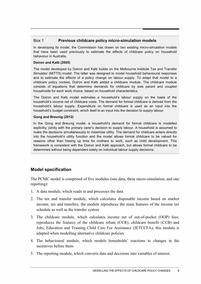
Box 1 Previous childcare policy micro-simulation models In developing its model, the Commission has drawn on two existing micro-simulation models that have been used previously to estimate the effects of childcare policy on household behaviour in Australia.
Doiron and Kalb (2005)
The model developed by Doiron and Kalb builds on the Melbourne Institute Tax and Transfer Simulator (MITTS) model. The latter was designed to model household behavioural responses and to estimate the effects of a policy change on labour supply. To adapt that model to a childcare policy context, Doiron and Kalb added a childcare module. The childcare module consists of equations that determine demands for childcare by sole parent and coupled households for each work choice, based on household characteristics.
The Doiron and Kalb model estimates a household’s labour supply on the basis of the household’s income net of childcare costs. The demand for formal childcare is derived from the household’s labour supply. Expenditure on formal childcare is used as an input into the household’s budget constraint, which itself is an input into the decision to supply labour.
Gong and Breunig (2012)
In the Gong and Breunig model, a household’s demand for formal childcare is modelled explicitly, jointly with the primary carer’s decision to supply labour. A household is assumed to make the decisions simultaneously to maximise utility. The demand for childcare enters directly into the household’s utility function and the model allows formal childcare to be valued for reasons other than freeing up time for mothers to work, such as child development. This framework is consistent with the Doiron and Kalb approach, but allows formal childcare to be determined without being dependent solely on individual labour supply decisions.
Model specification
The PCMC model is comprised of five modules (one data, three micro-simulation, and one reporting):
1. A data module, which reads in and processes the data
2. The tax and transfer module, which calculates disposable income based on market income, tax and transfers; the module reproduces the main features of the income tax schedule as well as the transfer system
3. The childcare module, which calculates income net of out-of-pocket (OOP) fees; reproduces the features of the childcare rebate (CCR), childcare benefit (CCB) and Jobs, Education and Training Child Care Fee Assistance (JETCCFA); this module is adapted when modelling alternative childcare policies
4. The behavioural module, which models households’ reactions to changes in the incentives before them
5. The reporting module, which converts data and decisions into variables of interest.

4 CHILDCARE AND EARLY CHILDHOOD LEARNING - TECHNICAL SUPPLEMENT
Tax and transfer module
The tax and transfer module calculates net income given the rules of the Australian tax and transfer system, based on gross income and household characteristics. The income tax schedule, all aspects of income support for working age families (including, for example, Newstart Allowance, the Parenting Payment and the Disability Support Pension), Medicare Levy, Commonwealth Rent Assistance and Family Tax Benefit A and B2 are accounted for in this module. This module serves as an input into the behavioural module.
Childcare module
The module includes the rules that govern the existing CCB, CCR and JETCCFA, including the current income and activity tests for CCB and the annual per child cap on CCR. It also enables alternative income and activity tests for the recommended new single child-based payment, Early Care and Learning Subsidy (ECLS). Income net of out-of-pocket childcare costs to families is calculated based on family labour income and transfers, net of income taxes, for given household characteristics.3 This module also serves as an input into the household behavioural module.
Behavioural module
The model represents household decisions about work and childcare in response to a change in out-of-pocket childcare fees for sole parent and coupled households where the youngest child is aged between 0 and 12 years. The main results consist of a projected choice, for each household of:
• the number of hours of work supplied by the primary care giver (including whether to enter or leave the workforce)
• the number of hours of formal childcare demanded.
The decisions are modelled simultaneously, consistent with the methodology developed in Gong and Breunig (2012). The manner in which these decisions are made, and the constraints facing households, are described in appendix B.
The results at the household level are aggregated to obtain estimates of shifts in labour supply and demand for formal childcare at an aggregate level, and for particular demographic groups. Combined with a demand for labour and a supply for childcare services, the results can be used to estimate fiscal costs.
The behavioural module is specified to generate a decision that maximises each household’s utility. A household’s utility is assumed to be quadratic and driven by the 2 Using pre-2014 Budget parameter values. 3 The model holds constant income from sources other than hours worked (e.g. capital income is assumed
not to change as a result of childcare policies).
MODELLING THE EFFECTS OF CHILDCARE POLICY CHANGES 5
following variables (which are included in the utility function): household disposable income net of out-of-pocket childcare expenses; labour supply; childcare from the primary care giver; and use of formal and informal childcare. The exact terms in the household utility functions are detailed in appendix B.
Net disposable income after out-of-pocket childcare expenses
Households are modelled to derive utility from income, as it can be spent on goods and services. The model uses the household income from labour and transfers net of taxes and out-of-pocket childcare fees as the input into the utility function.
For tractability, the model only estimates the impact of a change in the net income of the primary carer; the hours worked and wage rate of the primary earner are assumed to be exogenous. Although the primary earner could reduce their hours worked as their partner increases them, simulations not detailed in this document (where the hours of the primary earner were allowed to vary) indicated that this effect is small.
Hours of labour supplied
Some households derive utility from reducing the hours worked by the primary carer, because that time can be used in other ways, including for leisure, caring for children, or other home production. Households derive utility from labour supplied by the primary carer (where the primary carer enjoys working, but the household can also derive disutility from hours working). Households are assumed to derive utility from working zero hours. The model includes a fixed cost associated with supplying labour (regardless of the hours chosen)4, such as travel and other costs (aside from childcare costs) associated with working.
Leisure and home production are not explicitly represented in the household utility function. However, households derive utility from income and from time spent caring for children directly. Given that each member of the household is subject to a 24 hours a day time constraint, leisure and home production are valued implicitly.
Childcare from the primary care giver
Households derive utility from caring for children at home. The amount of childcare provided by the primary carer appears directly in the household’s utility function.
4 This is represented by the intercept utility parameter associated with zero work.

6 CHILDCARE AND EARLY CHILDHOOD LEARNING - TECHNICAL SUPPLEMENT
Formal childcare
The number of hours of formal childcare used by a household appears indirectly in the utility function (representing, for example, the household’s valuation of educational or social development of childcare). This means that use of formal childcare can provide households with benefits beyond those from enabling the primary carer to work. For this reason, formal childcare and the income that it enables households to earn appear separately in the utility function.
The model contains three broad forms of childcare: formal childcare; maternal childcare; and informal childcare. Only two of the three forms are directly incorporated into the objective function, as the third would be superfluous. For the purposes of this model, formal childcare is determined by the other two forms of care (maternal and informal), a binding time constraint for the primary carer, a binding time constraint for care of the child, and the cost of formal childcare (which enters through the income term). The model could be respecified to include any pair of forms of care, and produce identical results.
Behaviour of households with multiple children
Households with multiple children are assumed to base labour supply and childcare hours demand decisions on the caring needs of the youngest child. That is, childcare for school age children mirrors the decision for the youngest child. For example, for a family with one pre-school- and one school-age child, if the younger child requires 40 hours per week of non-parental childcare, the older child would also require 40 hours of non-parental supervision/care (consisting of a combination of school, outside school hours care (OSHC) and informal care).
Substitution between formal and informal childcare
Formal childcare is specified as the residual care required, net of the household’s use of informal childcare and of the time spent with the primary carer. Informal care can come from a range of sources not explicitly represented in the model, including care by the primary earner, other family members, neighbours and friends. The costs associated with informal care are not observed, but must be accounted for. If no utility parameters governed the relative value placed on the different forms of care, households would source all non-maternal care from informal care (since maternal care is bound by the primary carer’s total time, and formal childcare has a financial cost). Constraints on maternal time and required total childcare, combined with utility parameters for maternal and informal childcare, ensure the model reproduces the observed data. Observed data show that as people work more, their use of formal care increases.
Figure 1 provides a stylised representation of the model at the household level. It breaks down the model into the separate modules detailed above. It also shows the components generated in each module, that are inputs to other modules, and how each of those inputs is calculated.

Figure 1 Stylised Productivity Commission Micro-simulation Childcare Modela
a The model contains 8 work choices (each in 8 hour increments) and 6 formal childcare choices (each in 10 hour increments) giving each household up to 48 (8x6) possible choices. OOP stands for ‘out-of-pocket’, fcc for ‘formal childcare’, mcc for ‘maternal childcare’, and icc for ‘informal childcare’.

8 CHILDCARE AND EARLY CHILDHOOD LEARNING - TECHNICAL SUPPLEMENT
The framework adopted
Rather than specify labour supply and childcare demand as a continuous range, where primary carers could adjust those decisions in infinitely small increments, care and work choices in the model are divided into blocks approximating observed values (for example, an individual is assumed to choose to work 8 or 16 hours, not 10.71 hours). Under this approach, primary carers can make a choice from a limited set of combinations of labour and childcare hours.
This approach has practical, computational advantages, does not compromise materially the accuracy of results, and offers a tractable way to model policies and outcomes that involve ‘discontinuities’ or non-linear relationships that would be challenging to specify and estimate in a model with continuous variables (Creedy and Kalb 2006). In the case of childcare policy and workforce participation, the tax and transfer system (as well as the CCB and CCR rules), are characterised by complex sliding scales and eligibility thresholds.
Furthermore, the characteristics of the labour and childcare markets mean that there is typically a limited number of part-time work and formal childcare combinations that the primary carer would be able to secure.
Labour supply and childcare demand options available to primary carers
Households are assumed to choose a level of the primary carer’s weekly supply of labour within the range of 0–56 hours, in 8-hour increments. That is, they can choose from eight options, including 0 hours. They can also choose one of six 10-hour increment options of formal childcare demanded in the range of 0–50 hours, including 0 hours. OSHC care is divided into 4-hour increments (up to a total of 20 hours per week), which is used in conjunction with 6 hours of school per day. Households can elect from 48 combinations of hours of labour supplied and formal childcare demanded.
Households can choose between long day care, family day care, OSHC, nannies and pre-school (where they do not already use pre-school for a 4 year old child). Under the base case of current childcare assistance arrangements, the choice of childcare type is determined by a household’s initial choice as described in the database; for new users, 98 per cent of households are randomly assigned to a care type, based on shares observed in the administrative data (by income group), and 2 per cent are assumed to use nannies.
While the introduction of subsidies for approved nannies would increase the use of nannies, the extent to which households entering the childcare market would start choosing to use nannies is unclear. The 2 per cent figure was chosen in the absence of any information about household response; it is larger than the proportion of nanny use observed in the Survey of Income and Housing. Due to the relatively high hourly cost of nannies, results show that nannies are typically chosen by families with 2 or more children.

MODELLING THE EFFECTS OF CHILDCARE POLICY CHANGES 9
In the model, a nanny can take care of up to four children under 5 years old at one time (mirroring the existing staff-to-child ratio for family day care). Only households where the youngest child was under 5 were assigned the option of using nannies (appendix B).
The full technical specification of the model is detailed in appendix B.
Data set and estimation
In addition to the administrative rules governing the CCB, CCR, JETCCFA and the broader tax and transfer system, the model integrates two data sets to establish the baseline, and obtain weights for subsequent aggregation of results:
• data from the ABS Survey of Income and Housing 2011-12 (SIH)
• administrative data about childcare fees by type of care used and location for 2011-12 which has been supplied by the Department of Education.
The SIH includes data for over 3000 households representative of sole and couple parent households in Australia.5 The data for each observation were combined with administrative childcare fee data for 1.29 million children, based on location. The procedures used to produce the model database are summarised in appendix A. A brief overview of the data sources is included in box 2.
Utility function and wage equation parameters were estimated for the PCMC model using the Commission’s database (appendix C). These parameter estimates reflect the latest data available to the Commission (2011-12), and match the PCMC model specification. The approach adopted in the estimation follows the approach used in Doiron and Kalb (2005).
5 The SIH covers urban and rural areas (excluding very remote areas) of Australia covering about
97 per cent of the population (ABS 2013a). The ABS (2013a) noted that while excluding very remote areas only has a minor impact on aggregate estimates, nearly a quarter of all households in the Northern Territory live in very remote areas.

10 CHILDCARE AND EARLY CHILDHOOD LEARNING - TECHNICAL SUPPLEMENT
Box 2 Data sources The micro-simulation model uses two data sources:
• The 2011-12 Survey of Income and Housing (ABS 2013b) contains key demographic and economic characteristics of residents in private dwellings across Australia. The model database focuses on a subsample of the survey describing lone and coupled parents. All variables except childcare price are derived from this subsample.
• An unpublished administrative childcare database (Department of Education 2011-12), which provides a comprehensive description of childcare use, price, location of service and subsidies (including CCR and CCB). The administrative database was used to provide the mean and standard deviation of childcare prices by geographic location and type of care.
Several observations were excluded from the model database. Specifically, observations that reported positive employee income and zero labour supply were removed. Similarly, observations that reported parents with no children were also removed. Following consultation with the ABS, observations that reported zero employee income and positive labour supply were attributed an imputed wage using the estimated wage equation (appendix C), because it was felt that the absence of a wage could be explained without assuming the household’s response to the survey was invalid.
The final model database contains 3030 households (comprising 628 lone parent and 2402 coupled parent families). The database contains variables describing income, labour supply, number of children, age of parents, occupation, industry of employment, location, educational attainment, transfer payments received, hours of childcare used and childcare prices faced for each household. Some households are dropped as part of the model calibration, where their behaviour is particularly inconsistent with the model theory (appendix B).
2 Assumptions, caveats and limitations
There are important caveats that need to be remembered when interpreting the results from the PCMC model. Among others, the following issues are most prominent.
1. Data: responses in the SIH might not be internally consistent, or questions could be misunderstood or answered incorrectly by participants. For example, some observations included zero hours worked and non-zero labour income (appendix A). The data were reconciled with the administrative data. However, these data too, could contain inaccuracies, in particular, where people are incentivised to overstate the number of hours worked, or to overstate the amount of childcare they use.
2. Unemployment benefits: The model assumes that people who stop working as a result of the policy change will claim the NewStart Allowance. In the SIH data, a number of seemingly eligible people do not claim unemployment benefits; as such, the assumed behaviour could overstate the number of people who claim NewStart.
3. Childcare demand: the childcare hour result is best interpreted as a shift in the demand for childcare. The model assumes that each individual can obtain as many hours of childcare as they want at the supply price they currently face. There is no representation of childcare supply response: there is no increasing cost of childcare, nor any capacity

MODELLING THE EFFECTS OF CHILDCARE POLICY CHANGES 11
constraints. To the extent that childcare availability is constrained at current supply prices, the labour supply response could be smaller than projected. If childcare prices were to increase, the returns to labour net of taxes and out-of-pocket costs would decrease and the labour supply response and childcare demand response would reduce accordingly.
4. Labour supply: the labour hour results represent a shift in the supply of labour from households included in the model. This is equivalent to assuming that each individual can work as many hours as they want at the current wage. There is no representation of the demand for labour from workers with children, or of the labour response of those outside the PCMC model (workers without children). Any employment projection is likely to be smaller than the projected labour supply shifts. To the extent that labour supply increases, the real wage might fall, which could reduce the quantity of labour supplied by other individuals in the economy (i.e. individuals not included in the PCMC model).
5. Tax impacts: There is no representation of the potential reductions in labour supply if taxes have to be increased to fund any increases in fiscal cost. To the extent that additional funding is required through additional taxes, labour supply responses among those modelled could be lower than in the model results, and could be negative from individuals not included in the model (those without children). Given the Commission’s recommended approach is within the same fiscal envelope (i.e. the net fiscal impact for government is small or zero) this impact is expected to be small.
6. Broader economic impacts: the projected shifts in labour supply and childcare demand can be interpreted as upper bounds on the estimated effects on employment and childcare use. Any GDP extrapolation based on these shifts is therefore best interpreted as an upper bound on the possible effects on GDP.6
3 Policy simulations
For each policy scenario, the model produces results that include:7
1. net change in the supply of labour
2. net change in demand for formal childcare
6 Further, GDP is not a measure of social welfare. Important components of social welfare that are relevant
to this policy are excluded from GDP. In particular, while formal childcare contributes to GDP as part of economic activity, informal and parental care (valued by households) are not accounted for, and nor is the value of home production or that of leisure, or the possible longer term benefits of improved child development associated with participation in some types of formal childcare. Similarly, GDP will include a measurable increase in those who move from the cash economy to the measured economy. Some of the longer-term benefits might appear as positive GDP effects in the long run, which is not reflected in the micro-simulation model.
7 Conditional on assuming no changes in wages and no changes in childcare fees, and that childcare services and employment are available at any quantity at current prices.

12 CHILDCARE AND EARLY CHILDHOOD LEARNING - TECHNICAL SUPPLEMENT
3. ECEC costs to government, changes in income tax collections, changes in transfer payments, and the net impact on the government’s fiscal position
4. a range of aggregations for the impacts on various cohorts for labour supply, childcare demand, out-of-pocket expenses, effective subsidy rates.
Given the uncertainty surrounding the data and parameter values, results include ranges. The sensitivity tests varied the utility parameters based on the distributions from the econometric estimations and the variance-covariance matrixes (appendix B). Sensitivity ranges were constructed based on 1000 simulations.
The Commission has used the micro-simulation model to examine several alternative variants of early childhood subsidy arrangements recommended in the inquiry report. Each of these ECLS variants include:
1. A simplified assistance scheme replacing existing childcare subsides with a single payment (means tested against household income), calculated as a percentage of a benchmark price of childcare.
2. The benchmark price is set per hour of childcare.8 The benchmark price varies by type of care (long day care, home based care (including family day care and approved nannies), and OSHC). For long day care, the benchmark price also varies with the child age — 0 to 35 months and 36 months to primary school age. A household cannot receive a subsidy in excess of childcare fees.9
3. A new activity test for childcare assistance eligibility. At present, the CCB has no activity test for households claiming 24 hours or less of childcare a week; households must meet an activity test (15 hours a week) to receive a subsidy for childcare hours in excess of 24 hours per week. The CCR simply requires that each parent be working/training/studying/seeking work/volunteering to be eligible. The scenarios institute a single fortnightly activity test on each parent in the household to be eligible for formal childcare assistance (not including pre-school).10
8 The benchmark price was set such that it is less/more than the actual childcare fees paid by approximately
50 per cent of the households in the population. 9 Two possible specifications were examined for subsidy payments relative to the benchmark price for the
case where the dollar subsidy (subsidy rate applied to the benchmark price) exceeds childcare fees. In the first case, the dollar subsidy is reduced to 100 per cent of the childcare fee. In the second case, the subsidy is calculated on the basis of the scheduled rate. The ‘scheduled rate’ refers to the rate of the benchmark price that would be subsidised, as opposed to the share of the childcare fee that is actually subsidised.
10 The activity test is applied for all families other than for grandparents or other non-parental primary carers, when parents receive a Disability Support Pension or Carer Payment (other than for the child using the ECEC service), when children are assessed to be at risk, or in exceptional circumstances including due to a loss of a job for a short period. These exemptions to the activity test were not included in the draft report modelling. Variations of activity tests that were modelled include a 16 hour fortnightly test, a 24 hour fortnightly test, as well as either a 10 hour or complete exemption for households receiving the Parenting Payment.

MODELLING THE EFFECTS OF CHILDCARE POLICY CHANGES 13
The policy recommendations in the inquiry report examined in this technical supplement includes (figure 2):
1. A 24-hour fortnightly activity test for all members of a household enabling the household to receive up to 100 hours per fortnight of subsidised care. Households receiving the Parenting Payment can access up to 20 hours per fortnight of subsidised care without passing the activity test.
2. Assistance at 85 per cent of the benchmark price for households with gross income less than $60 000.
3. Assistance at 20 per cent of the benchmark price for households with gross income at or above $250 000
4. Subsidy rates for households with a gross income between $60 000 and $250 000 are calculated using a linear taper rate. For example, a household with an income of $100 000 would receive 71 per cent of the benchmark price.
5. The benchmark price is set equal to the median fee paid as reported in the administrative data. Households can receive, at most, a 100 per cent subsidy where their subsidy rate times the benchmark price exceeds the childcare price they face.
Figure 2 Schedule of subsidy rates under ECLSa
a ECLS replaces existing childcare subsidies with a single means tested subsidy rate applied to a benchmark price base.
0
20
40
60
80
100
0 100000 200000 300000 400000 500000
Perc
enta
ge o
f ben
cham
ark
pric
e pa
id a
s su
ibsi
dy
Household income range ($/year)

14 CHILDCARE AND EARLY CHILDHOOD LEARNING - TECHNICAL SUPPLEMENT
4 Model results, mechanisms and drivers
Table 1 presents illustrative results ranges, as well as the ‘central’ result for the simulation based on the estimated parameters (appendix C). The ranges were constructed by defining ranges around these parameters based on the variance-covariance matrixes taken from the econometric estimation of the model utility functions (appendix B). Simulations were completed with different parameter values — 1000 simulations, drawing parameter value sets using the variance-covariance matrixes from the estimation. The ‘lower bounds’ and ‘upper bounds’ cover 95 per cent of the results obtained from the 1000 simulations.
Unless stated otherwise, model results for labour supply are couched in terms of shifts in aggregate national labour supply — that is, the increase in total hours (or FTEs) in the economy from those primary carers changing their labour supply decision in the PCMC model.
Table 1 shows that the results are sensitive to parameter values. Results for childcare demand are somewhat more sensitive than those for labour supply. Total ECEC cost is largely driven by childcare demand, while changes in government transfers and tax receipts are driven by labour response, making the net fiscal implications more complex to analyse, but still close to neutral.
In general, increasing subsidy payments increases demand for childcare, and the supply of labour hours. Higher income households who receive reduced subsidies tend not to change their behaviour much — to an extent, high income households (as shown in the data) are willing to fund childcare out-of-pocket, and make a labour supply decision that is not heavily dependent on their level of childcare subsidy. Low- and middle-income households who receive higher subsidy rates respond by increasing their demand for childcare and their supply of labour. Households that are impacted by the activity test tend to either increase their labour supply, or stop demanding care; in aggregate, they increase labour supply and reduce net fiscal costs.
There is potentially a small net fiscal cost for government associated with the Commission’s recommendations as a whole, as income tax and transfer payment changes from increased labour supply do not completely offset the additional childcare subsidy expense. However, the range indicates that the net fiscal impact is likely to be close to zero.
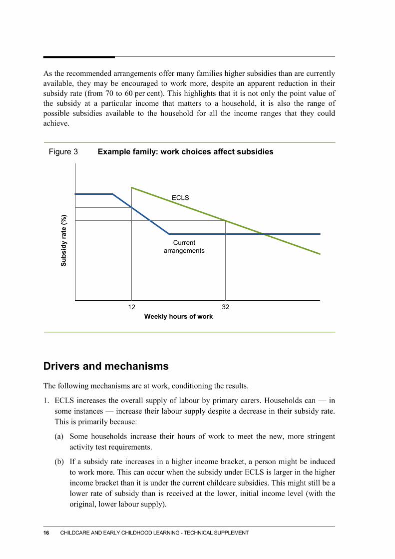
It is also worth noting that for some individuals, it can appear that despite an apparent reduction in their rate of childcare subsidy their childcare demand and labour supply can increase. This is because people shift between income groups — reporting is based on initial income, but some households will supply more labour and earn more post-policy change — as illustrated using an example family (figure 3). A primary carer may initially choose to work 12 hours per week and be eligible for a subsidy rate of 70 per cent (when CCB and CCR entitlements are combined). Alternatively, they could work for 32 hours a week. Under the current CCB and CCR arrangements, due to the means testing of the CCB
MODELLING THE EFFECTS OF CHILDCARE POLICY CHANGES 15
subsidy rate, they would only receive the 50 per cent CCR subsidy if they worked 32 hours a week (assuming they have not reached the CCR cap). Under ECLS, the subsidy rate at 32 hours could be 60 per cent for this person.
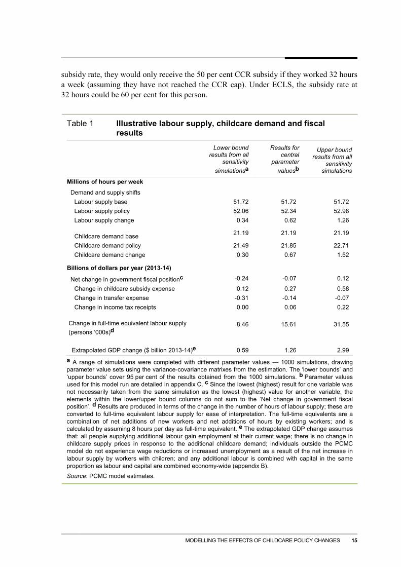
Table 1 Illustrative labour supply, childcare demand and fiscal
results
Lower bound results from all
sensitivity simulationsa
Results for central
parameter valuesb
Upper bound results from all
sensitivity simulations
Millions of hours per week Demand and supply shifts
Labour supply base 51.72 51.72 51.72 Labour supply policy 52.06 52.34 52.98 Labour supply change 0.34 0.62 1.26
Childcare demand base 21.19 21.19 21.19
Childcare demand policy 21.49 21.85 22.71 Childcare demand change 0.30 0.67 1.52
Billions of dollars per year (2013-14)
Net change in government fiscal positionc -0.24 -0.07 0.12
Change in childcare subsidy expense 0.12 0.27 0.58 Change in transfer expense -0.31 -0.14 -0.07 Change in income tax receipts 0.00 0.06 0.22
Change in full-time equivalent labour supply (persons ‘000s)d
8.46 15.61 31.55
Extrapolated GDP change ($ billion 2013-14)e 0.59 1.26 2.99
a A range of simulations were completed with different parameter values — 1000 simulations, drawing parameter value sets using the variance-covariance matrixes from the estimation. The ‘lower bounds’ and ‘upper bounds’ cover 95 per cent of the results obtained from the 1000 simulations. b Parameter values used for this model run are detailed in appendix C. c Since the lowest (highest) result for one variable was not necessarily taken from the same simulation as the lowest (highest) value for another variable, the elements within the lower/upper bound columns do not sum to the ‘Net change in government fiscal position’. d Results are produced in terms of the change in the number of hours of labour supply; these are converted to full-time equivalent labour supply for ease of interpretation. The full-time equivalents are a combination of net additions of new workers and net additions of hours by existing workers; and is calculated by assuming 8 hours per day as full-time equivalent. e The extrapolated GDP change assumes that: all people supplying additional labour gain employment at their current wage; there is no change in childcare supply prices in response to the additional childcare demand; individuals outside the PCMC model do not experience wage reductions or increased unemployment as a result of the net increase in labour supply by workers with children; and any additional labour is combined with capital in the same proportion as labour and capital are combined economy-wide (appendix B).
Source: PCMC model estimates.
16 CHILDCARE AND EARLY CHILDHOOD LEARNING - TECHNICAL SUPPLEMENT
As the recommended arrangements offer many families higher subsidies than are currently available, they may be encouraged to work more, despite an apparent reduction in their subsidy rate (from 70 to 60 per cent). This highlights that it is not only the point value of the subsidy at a particular income that matters to a household, it is also the range of possible subsidies available to the household for all the income ranges that they could achieve.
Figure 3 Example family: work choices affect subsidies
Drivers and mechanisms
The following mechanisms are at work, conditioning the results.
1. ECLS increases the overall supply of labour by primary carers. Households can — in some instances — increase their labour supply despite a decrease in their subsidy rate. This is primarily because:
(a) Some households increase their hours of work to meet the new, more stringent activity test requirements.
(b) If a subsidy rate increases in a higher income bracket, a person might be induced to work more. This can occur when the subsidy under ECLS is larger in the higher income bracket than it is under the current childcare subsidies. This might still be a lower rate of subsidy than is received at the lower, initial income level (with the original, lower labour supply).
Subs
idy
rate
(%)
ECLS
Current arrangements
12 32Weekly hours of work
MODELLING THE EFFECTS OF CHILDCARE POLICY CHANGES 17
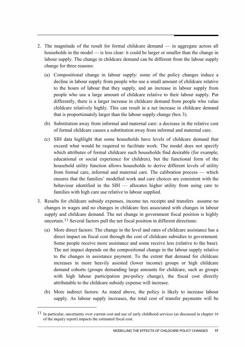
2. The magnitude of the result for formal childcare demand — in aggregate across all households in the model — is less clear: it could be larger or smaller than the change in labour supply. The change in childcare demand can be different from the labour supply change for three reasons:
(a) Compositional change in labour supply: some of the policy changes induce a decline in labour supply from people who use a small amount of childcare relative to the hours of labour that they supply, and an increase in labour supply from people who use a large amount of childcare relative to their labour supply. Put differently, there is a larger increase in childcare demand from people who value childcare relatively highly. This can result in a net increase in childcare demand that is proportionately larger than the labour supply change (box 3).
(b) Substitution away from informal and maternal care: a decrease in the relative cost of formal childcare causes a substitution away from informal and maternal care.
(c) SIH data highlight that some households have levels of childcare demand that exceed what would be required to facilitate work. The model does not specify which attributes of formal childcare such households find desirable (for example, educational or social experience for children), but the functional form of the household utility function allows households to derive different levels of utility from formal care, informal and maternal care. The calibration process — which ensures that the families’ modelled work and care choices are consistent with the behaviour identified in the SIH — allocates higher utility from using care to families with high care use relative to labour supplied.
3. Results for childcare subsidy expenses, income tax receipts and transfers assume no changes in wages and no changes in childcare fees associated with changes in labour supply and childcare demand. The net change in government fiscal position is highly uncertain.11 Several factors pull the net fiscal position in different directions:
(a) More direct factors: The change in the level and rates of childcare assistance has a direct impact on fiscal cost through the cost of childcare subsidies to government. Some people receive more assistance and some receive less (relative to the base). The net impact depends on the compositional change in the labour supply relative to the changes in assistance payment. To the extent that demand for childcare increases in more heavily assisted (lower income) groups or high childcare demand cohorts (groups demanding large amounts for childcare, such as groups with high labour participation pre-policy change), the fiscal cost directly attributable to the childcare subsidy expense will increase.
(b) More indirect factors: As stated above, the policy is likely to increase labour supply. As labour supply increases, the total cost of transfer payments will be
11 In particular, uncertainty over current cost and use of early childhood services (as discussed in chapter 16
of the inquiry report) impacts the estimated fiscal cost.

18 CHILDCARE AND EARLY CHILDHOOD LEARNING - TECHNICAL SUPPLEMENT
reduced (for example, means-tested family tax benefits are reduced as earnings increase). Further, as people work more, income tax collections increase.
Box 3 Illustrations of compositional change and aggregate results The micro-simulation model aggregates heterogeneous household level responses to produce aggregate results. In a number of cases, this aggregation can produce results that appear counter intuitive. In particular, this occurs where there are either (a) changes in the patterns of childcare use among workers; or (b) differential responses within a group.
(a) Changes in patterns of childcare use among workers
Assume person A is initially supplying 16 labour hours and demanding 10 childcare hours per week, while person B is initially out of the labour force. Further assume that a policy change causes person A to drop out of the labour force (and cease demanding childcare), while person B starts working. Person B starts supplying 24 labour hours and demanding 20 childcare hours.
The aggregate change (across person A and B) is an additional 8 hours (24 – 16) of labour supply with an additional 10 hours (20 – 10) of childcare demand per week. In aggregate, it appears that a large amount of additional childcare is required to induce a relatively small amount of additional labour supply.
(b) Differential responses within a group
If individuals within a group experience different changes, the aggregate results can exhibit counter intuitive results. Person C might get a large reduction in their childcare subsidy ($1000), but might only reduce their labour supply by a small amount (8 hours per week). Person D might get only a small increase in their subsidy ($200), but increase their labour supply by a larger amount (16 hours per week).
The aggregate change (across persons C and D) is an aggregate decrease in $800 subsidy ($1000 – $200) and an aggregate 8 hour increase in labour supply. While this aggregate result may appear counter intuitive, it is based on expected behaviour at the household level.
Understanding the following interactions in the model can help explain the results:
1. The activity test has a positive impact on labour supply. The database contains a number of people (about 2.5 per cent of households) who initially work fewer hours than required under the proposed activity test, use some childcare, and are not exempted from the proposed activity test for reasons such as pursuing education. These households face an incentive to increase their work hours to meet the activity test (or lose their childcare subsidy). This incentive exists even for households where the subsidy rate (once the activity test is met) is reduced. For this reason, the labour supply response for households that face a lower subsidy rate can be positive — this effect is driven by the activity test. The work test causes an increased concentration of subsidies accruing to those using childcare for work purposes, and encourages those working fewer hours to increase their work hours or drop out of the childcare market entirely (or reduce their childcare demand to 10 hours per week if they receive the Parenting Payment).

MODELLING THE EFFECTS OF CHILDCARE POLICY CHANGES 19
2. Relatively high income groups receive less assistance and their disposable income net of out-of-pocket fees is reduced. This is because the CCR subsidy (50 per cent of childcare costs, up to $7500 per child per year) is replaced by the lower subsidy of 20 per cent of the benchmark price. Some work less as a result, although some substitute towards/using more informal care or increasing out-of-pocket expenditure on formal childcare and maintaining hours worked. The utility of this group is reduced: high income households are relatively unresponsive to reduced assistance (compared to other income groups), opting to fund their relatively fixed use of childcare through increased out-of-pocket spending.
3. Half of families have childcare fees that exceed the benchmark price. For these families, the effective subsidy rate is lower than it appears from the rate schedule, because the benchmark price to which the rate applies is below the childcare fee they face. This increases the possibility that the effective subsidy rate is lower than under current arrangements. Such households typically reduce their childcare demand and labour supply. Note that the micro-simulation framework does not account for any supply-side changes that could be induced by reduced subsidies, so any changes in out-of-pocket childcare fees brought about by switching to the benchmark price approach are assumed to be borne by — or to benefit — households.12
4. The primary financial beneficiaries of the policy change are low- and middle-income households. While the simplified system tends to cut assistance to the upper-income groups (and some people affected by the new activity test), payments to the low- and middle-income groups tend to increase relative to current arrangements. While some households experience a decrease in other transfers as they increase their labour supply, the new childcare subsidies more than compensate for this loss, resulting in a net increase in government payments to that group. Some middle- and high- income households who would hit the $7500 CCR cap if they worked more than 2-3 days per week could also benefit financially from the policy change as the net return from working more than 2-3 days may be higher under the new subsidy arrangements. The new arrangements are not capped.
5. There is a substitution away from non-market childcare (parental and informal) in favour of formal childcare. Not all increases in childcare demand are driven by increased labour supply. As the out-of-pocket costs of childcare decrease for some households (mainly low- and middle-income), they increase their use of childcare. This means that there is not a one-to-one correspondence between increases in childcare hours and increases in labour supply hours for all groups in the model. The relative price decrease of formal childcare causes a substitution away from informal care and towards formal care.
12 It can be argued that the benchmark price could place downwards pressure on prices charged by higher
cost providers. Similarly, the benchmark price could provide incentives for lower cost providers to increase their prices to the benchmark price.
20 CHILDCARE AND EARLY CHILDHOOD LEARNING - TECHNICAL SUPPLEMENT
Decomposition of model results
This section illustrates the intuition behind the micro-level responses seen in the model. This is followed by a decomposition of model results. The section concludes with the utility payoff matrixes for an example household under the current arrangements and under the Commission’s recommended policy to illustrate the mechanisms at work.
Intuition underlying the micro-level behaviour
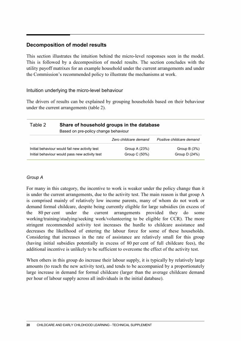
The drivers of results can be explained by grouping households based on their behaviour under the current arrangements (table 2).
Table 2 Share of household groups in the database
Based on pre-policy change behaviour
Zero childcare demand Positive childcare demand
Initial behaviour would fail new activity test Group A (23%) Group B (3%) Initial behaviour would pass new activity test Group C (50%) Group D (24%)
Group A
For many in this category, the incentive to work is weaker under the policy change than it is under the current arrangements, due to the activity test. The main reason is that group A is comprised mainly of relatively low income parents, many of whom do not work or demand formal childcare, despite being currently eligible for large subsidies (in excess of the 80 per cent under the current arrangements provided they do some working/training/studying/seeking work/volunteering to be eligible for CCR). The more stringent recommended activity test increases the hurdle to childcare assistance and decreases the likelihood of entering the labour force for some of these households. Considering that increases in the rate of assistance are relatively small for this group (having initial subsidies potentially in excess of 80 per cent of full childcare fees), the additional incentive is unlikely to be sufficient to overcome the effect of the activity test.
When others in this group do increase their labour supply, it is typically by relatively large amounts (to reach the new activity test), and tends to be accompanied by a proportionately large increase in demand for formal childcare (larger than the average childcare demand per hour of labour supply across all individuals in the initial database).
MODELLING THE EFFECTS OF CHILDCARE POLICY CHANGES 21
Group B
Individuals in group B tend to respond in one of two ways: they either increase their labour supply hours to meet the new activity test level (or higher); or remain at low/zero labour supply and cut their childcare demand.
Despite its small size (3 per cent of households), this group makes a large contribution to overall outcomes in terms of labour supply and of net fiscal impacts. In particular, those who increase their labour supply to meet (or exceed) the number of working hours required to satisfy the new activity test are significant contributors to the total increase in labour supply.
Since nearly everyone in group B has access to childcare subsidies in the initial data, the activity test makes those who do not change their behaviour unambiguously worse off (because they will be working and using the same amount of childcare, but will be paying more for that care if they are not eligible for ECLS).
However, those who receive a higher rate of assistance than before and change their behaviour (this is, allowing other factors besides the activity test to vary) can experience either an increase or decrease in their utility. In particular, utility can increase for a household if subsidy rates have become more favourable by sufficient magnitude that the rate change alone would have been sufficient to induce them to their higher level of activity (i.e. the new activity test is not what is changing their behaviour). To the extent that any subsidy increase (or, considering the new benchmark price arrangements, subsidy decrease) is not sufficient to induce additional labour supply, these households will experience a decrease in utility if the activity test induces them to supply additional labour.
Individual characteristics (such as education, age and current wage) are important for this group, and influence the nature of the tradeoff between childcare and work for the household. The tradeoff between maintaining the pre-policy level of childcare and working (governed by utility parameters) plays a key role in determining their decision.
This is the group most likely to improve the government’s net fiscal position. Either they:
• increase labour supply while maintaining a relatively stable level of childcare demand. In this case transfers decrease, income tax receipts increase and subsidy costs remain relatively stable, or
• maintain a low level of labour supply and reduce their demand for childcare services (since they are no longer eligible for the subsidy). In this case, transfers and income tax collections remain relatively unchanged and the subsidy cost is reduced.
The activity test is a significant contributor to labour supply and the improvement in the net fiscal position (this is illustrated quantitatively below). In scenarios where the fiscal position improves, it is because the fiscal savings from the activity test combined with savings from reduced payments to high income earners more than offset any increases in childcare subsidies to other groups. To the extent that the activity test hours are reduced or

22 CHILDCARE AND EARLY CHILDHOOD LEARNING - TECHNICAL SUPPLEMENT
more exemptions are granted beyond those on a parenting payment, the cost of any scheme increases.
The 10-hour per week childcare exemption for Parenting Payment recipients reduces the negative impact on low income households that do not change their hours of work to meet the activity test. However, this also mutes the labour supply response from the lowest income households.13
Groups C and D
Groups C and D are the most responsive to changes in the rate of assistance and are largely unaffected by the activity test. For those households who experience cuts in their rate of assistance, they typically:
1. do not change their choices but experience lower utility (due to lower income net of taxes and out-of-pocket fees), or
2. use more informal care, or
3. reduce their hours of labour supply to be at or slightly above the activity test.
Households that experience an increase in the rate of assistance tend not to be a large source of additional labour supply compared with groups A and B. In general, households in groups C and D already supply labour under the current arrangements (some pass the activity test by studying). Decreasing out-of-pocket fees increases net returns to labour, which (other things equal) will increase the supply of labour. However, because they are already supplying labour, their marginal change is unlikely to be as large as a primary carer making the decision to start supplying labour.
Many in group D are already at the CCR cap under the current arrangements. For some, the new arrangements increase the rate of assistance they receive, which increases childcare subsidy expenses to government. For example, a high income household that spends a very large amount on childcare could hit the $7500 CCR cap, but this could be a smaller amount than their total hours of care multiplied by 20 per cent (the new, lowest rate) of the benchmark price.
Illustrative decomposition of model results
This section uses the four groups and intuition in the previous section to explain the illustrative results for the recommended subsidy arrangements detailed in section 3 above. Given the parameter and data limitations discussed previously these results should be considered illustrative of the potential impacts of ECLS.
13 The impact of the Parenting Payment activity test exemption, as well as the activity test more broadly, is
covered in greater detail in the section 5.

MODELLING THE EFFECTS OF CHILDCARE POLICY CHANGES 23
In order to illustrate the impact of the activity test separately from the changes in the subsidy rates, it is useful to first decompose the aggregate model results by the four groups discussed above (table 3).
Table 3 Contribution to illustrative results by each group
Group A Group B Group C Group D Total
Initial childcare demand Zero Non-zero Zero Non-zero Pass or fail new activity test based on original behaviour
Fail Fail Pass Pass
Mean annual income net of taxes and out-of-pocket childcare fees ($) 85 169 75 321 80 613 78 588
Mean weekly hours worked by the primary carer (hours) 2.57 3.51 19.66 23.25
Millions of hours per week
Initial demand and supply (hours) Labour supply 1.89 0.28 31.50 18.05 51.72 Childcare demand 0.00 1.52 0.00 19.67 21.19
Demand and supply shifts (hours) Labour supply 0.21 0.31 0.10 0.00 0.62 Childcare demand 0.33 -0.11 0.71 -0.27 0.67
Billions of dollars per year (2013-14)
Contributions to fiscal positiona
Childcare subsidy expense 0.10 -0.17 0.20 0.14 0.27 Transfer expenses -0.04 -0.07 -0.02 -0.01 -0.14 Income tax receipts 0.01 0.04 0.00 0.01 0.06
Change in fiscal positionb -0.05 0.29 -0.18 -0.13 -0.07
Change in full-time equivalent labour supply (persons ‘000s)
5.36 7.69 2.60 -0.03 15.61
a Holding wages and childcare fees constant. b May not add up due to rounding.
Source: PCMC model estimates.
Table 3 shows that the majority of the aggregate labour supply increase comes from people who initially supply low levels of labour and would initially fail the new activity test (groups A and B, increasing labour supply by 0.21 and 0.31 million hours per week respectively), and that the majority of the fiscal savings comes from people who are affected by the new activity test and initially use childcare (group B, with a net fiscal position improvement of $0.29 billion per year).
People with no initial childcare demand benefit from the subsidy rate increases and changes to the activity test (groups A and C, receiving additional ECEC subsidies of 0.10 billion and 0.20 billion per year). This is reflected in their large increase in childcare
24 CHILDCARE AND EARLY CHILDHOOD LEARNING - TECHNICAL SUPPLEMENT
demand (0.33 and 0.71 million hours per week respectively). While there are reductions in other transfer payments ($0.04 and $0.02 billion per year for group A and B respectively), net government transfers to both groups increase (by $0.05 and 0.18 billion per year respectively).
Group B reduce their aggregate childcare demand under the recommended arrangements. As discussed above, the new activity test makes people in this group either (i) start working/work more to satisfy the activity test or (ii) reduce their childcare demand. Both choices improve the government’s fiscal position, by respectively (i) reducing transfer payments ($0.07 billion per year) and increasing income tax revenue slightly ($0.04 billion per year) or (ii) decreasing childcare subsidy payments ($0.17 billion per year).
Groups C and D contribute to increasing fiscal costs ($0.18 and $0.13 billion per year respectively). The drivers of these expenses are different for the two groups.
• Group C — who increase their labour supply (0.10 million hours per week) by a small proportion compared to their childcare demand increase (0.71 million hours per week) — substitute towards formal care and away from informal care due to the relative decrease in the out-of-pocket prices they face. Since this is not driving a large labour supply response, the government ECEC expense is not materially offset by any increases in income tax revenue collections or transfer payments savings.
• Group D have two compositional effects. First, high income households reduce their demand for childcare (see next section). Second, households that already use childcare and receive more favourable subsidy rates under the new arrangements receive higher subsidies on their base-level demand for childcare. Neither group changes their labour supply in any material way as a result of the policy change.
• In general, the results indicate that a large share of additional labour supply comes from people with no or low initial labour supply (groups A and B), while a large share of the fiscal costs comes from households with pre-existing labour supply (groups C and D).
Impacts by income groups
The impact of ECLS can be disaggregated based on the income ranges of households pre-policy (table 4).

MODELLING THE EFFECTS OF CHILDCARE POLICY CHANGES 25
Table 4 Illustrative impacts on labour supply, childcare demand, and
childcare subsidy cost by gross household income
Household income range
Share of households
(%)
Change in full time
equivalent workersa
(‘000s)
Change in labour
supply (millions of hours per
week)
Change in childcare demand
(millions of hours per
week)
Change in total childcare
subsidyb,c ($m per
week)
Under 40 000 21.99 3.22 0.13 0.12 1.94 40 000 to 60 000 14.73 3.86 0.15 0.05 -0.30 60 000 to 80 000 11.33 5.61 0.22 0.18 1.18 80 000 to 100 000 12.24 3.74 0.15 0.14 0.84 100 000 to 130 000 15.10 0.82 0.03 0.19 4.69 130 000 to 160 000 10.92 -0.33 -0.01 0.09 0.53 160 000 to 200 000 7.20 -0.29 -0.01 0.04 -0.70 200 000 to 300 000 4.90 -0.58 -0.02 -0.10 -1.92 Above 300 000 1.60 -0.41 -0.02 -0.04 -1.14
a Full-time equivalent workers is calculated by assuming 8 hours per day as full-time equivalent. b Holding wages and childcare fees constant. c Note that it is possible for there to be large changes in childcare subsidies but small changes in the quantity demanded due to compositional shifts within the group (box 3).
Source: PCMC model estimates.
Table 4 illustrates impacts in three broad categories:
1. Households with gross incomes above $160 000 decrease their labour supply by a small amount in response to the policy change. However, they contribute fiscal savings from reduced childcare subsidies ($3.76 million per week).14
2. Some low income households (with incomes between $40 000 and $60 000) increase their labour supply slightly (0.15 million hours per week) and cause a government childcare expenditure saving ($0.30 million per week). This effect is driven largely by the new activity test, which causes some people to cut their demand for formal childcare. This group is most affected by the activity test because (a) there are many households in the group who do not work enough to qualify for assistance and (b) a lower proportion are eligible for the Parenting Payment activity test exemption relative to the lowest income group.
3. Other households produce an aggregate increase in labour supply (summing to 0.52 million hours per week) and a large increase in formal childcare demand
14 The labour supply decrease in the top two income brackets are driven by two factors: 1) a small number of
observations in that cohort; 2) compositional change, as some within the group receive less favourable subsidies and decrease labour supply (typically households hitting the $7500 CCR limit under current arrangements who receive a subsidy rate of at least 20 per cent of the benchmark price under the new arrangements), while others within the group receive lower rates of assistance, but do not reduce work (instead funding formal childcare out-of-pocket).

26 CHILDCARE AND EARLY CHILDHOOD LEARNING - TECHNICAL SUPPLEMENT
(summing to 3.9 million hours per week). This group is the major source of increased fiscal expenditure (having an additional childcare subsidy cost of $9.18 million per week). The groups that contribute the largest increases in ECEC expenditure are:
(a) Households with an income between $100 000 and $130 000, because they are likely to pass the activity test (many households in this class are couples with two working parents), and benefit from increased subsidy rates in the middle of the decreasing taper under ECLS.
(b) Households with incomes under $40 000, who receive larger subsidies, and typically are exempt from the activity test by reason of Parenting Payment or other exemptions (such as, receiving a Disability Support Pension or studying).
An illustration example of the decision making process in the model
While it is not possible to investigate the responses by all households, it is instructive to analyse how incentives change for an example observation. Table 5 shows some characteristics for an example household from group D, both pre- and post-policy change. This household is assumed to face relatively low fees (below the benchmark price), and therefore receives an effective subsidy of 100 per cent under the recommended arrangements. Note that this household is just an example, and not representative of all responses in the model. The purpose of micro-simulation is to represent population heterogeneity, as such, no one agent is representative of the behaviour of any other agent in the data.
Table 5 Illustrative results for an example household
Primary carer’s hours of
labour supply per week
Childcare hours demanded per week
Subsidy rate as a
proportion of unit childcare
cost
Gross labour income per
week
Income net of tax and transfers
per week
Pre-policy 32 20 88% $692 $826 Post-policy 48 40 100%a $1 039 $1 026
a. This household is paying childcare fees (pre-subsidy) below the benchmark price. This is why their subsidy rate (100%) is larger than the upper bound on rate (85%) shown in figure 2.
Source: PCMC model estimates.
Increasing the subsidy decreases out-of–pocket childcare fees. For a given level of labour supply, the household’s utility level has increased (due to the larger amount of income net of taxes and out-of-pocket fees). Reduced out-of-pocket fees also reduce the costs of working and increases labour supply, along with the demand for childcare services.
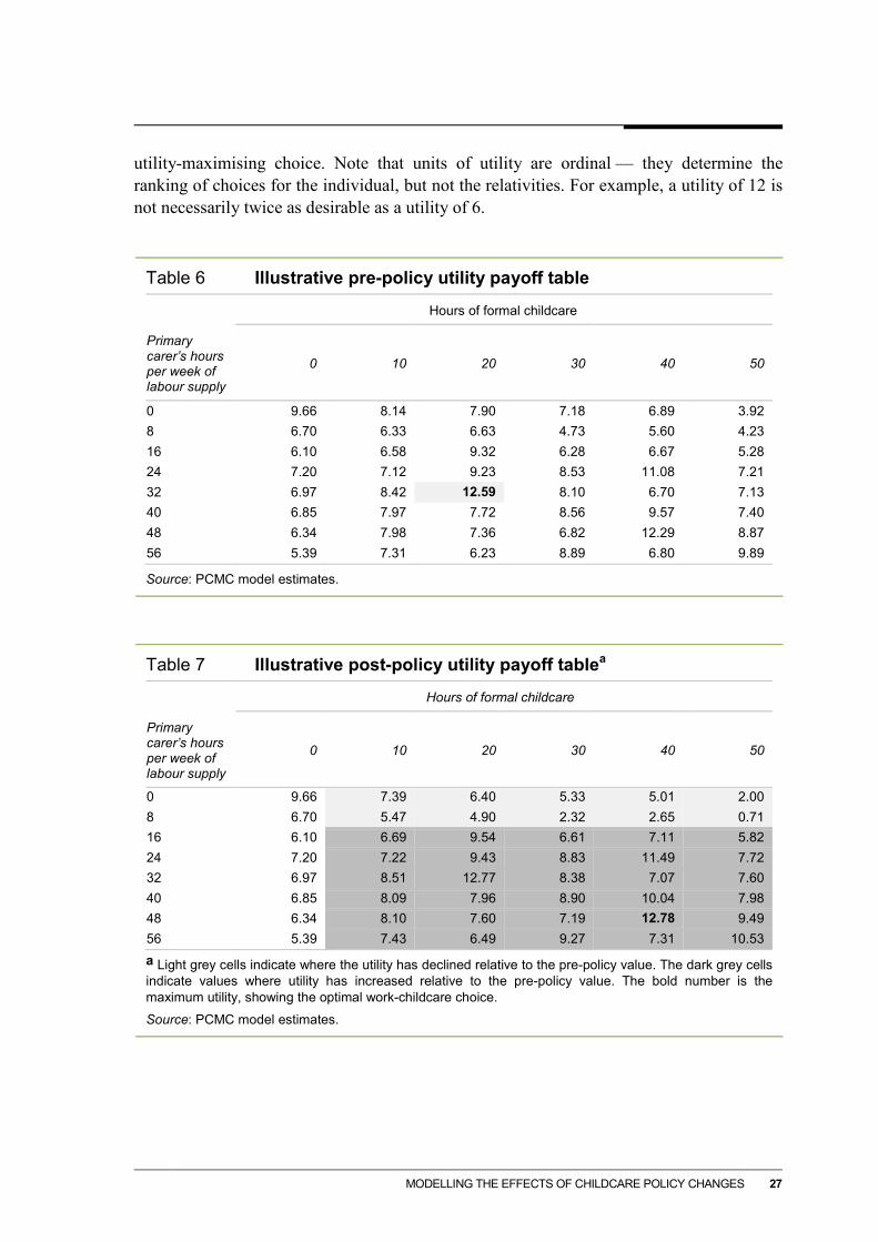
The utility the household derives from all possible work/childcare decisions pre- and post-policy change are shown in tables 6 and 7. The cells with bold text indicate the
MODELLING THE EFFECTS OF CHILDCARE POLICY CHANGES 27
utility-maximising choice. Note that units of utility are ordinal — they determine the ranking of choices for the individual, but not the relativities. For example, a utility of 12 is not necessarily twice as desirable as a utility of 6.
Table 6 Illustrative pre-policy utility payoff table
Hours of formal childcare
Primary carer’s hours per week of labour supply
0 10 20 30 40 50
0 9.66 8.14 7.90 7.18 6.89 3.92 8 6.70 6.33 6.63 4.73 5.60 4.23 16 6.10 6.58 9.32 6.28 6.67 5.28 24 7.20 7.12 9.23 8.53 11.08 7.21 32 6.97 8.42 12.59 8.10 6.70 7.13 40 6.85 7.97 7.72 8.56 9.57 7.40 48 6.34 7.98 7.36 6.82 12.29 8.87 56 5.39 7.31 6.23 8.89 6.80 9.89
Source: PCMC model estimates.
Table 7 Illustrative post-policy utility payoff tablea
Hours of formal childcare
Primary carer’s hours per week of labour supply
0 10 20 30 40 50
0 9.66 7.39 6.40 5.33 5.01 2.00 8 6.70 5.47 4.90 2.32 2.65 0.71 16 6.10 6.69 9.54 6.61 7.11 5.82 24 7.20 7.22 9.43 8.83 11.49 7.72 32 6.97 8.51 12.77 8.38 7.07 7.60 40 6.85 8.09 7.96 8.90 10.04 7.98 48 6.34 8.10 7.60 7.19 12.78 9.49 56 5.39 7.43 6.49 9.27 7.31 10.53
a Light grey cells indicate where the utility has declined relative to the pre-policy value. The dark grey cells indicate values where utility has increased relative to the pre-policy value. The bold number is the maximum utility, showing the optimal work-childcare choice.
Source: PCMC model estimates.

28 CHILDCARE AND EARLY CHILDHOOD LEARNING - TECHNICAL SUPPLEMENT
The individual has higher utility as a result of the policy even assuming no behavioural change (at 32 hours of labour supply, 20 hours of childcare demand per week). However, a higher ranking level of utility can be obtained by supplying 48 hours of labour, and using 40 hours of childcare.
5 Sensitivity of model results to alternative policy settings
As part of the inquiry process the Commission examined a range of alternative policy settings, including variations to the activity test and eligibility criteria, maximum subsidy payments with respect to the benchmark price, how the benchmark price is determined, as well as variation of the maximum and minimum subsidy rates. This section illustrates the impacts of alternative policy settings on aggregate results, and for different demographic groups. Different cut-offs15 were also examined, but are not illustrated here, as the insights from these variations are similar to those from other policy alternatives.
Activity test
The recommended subsidy arrangements include an activity test requiring at least 24 hours of work, study or training per fortnight (modelled as 12 hours per week) from each parent for a household to be eligible for assistance, with an exemption for up to 20 hours of subsidies care per fortnight (modelled as 10 hours of subsidised care per week) for households receiving the Parenting Payment. The Commission also examined scenarios without an activity test, with an 16 hour per fortnight activity test (modelled as 8 hours per week), as well as alternative levels of exemption for households receiving the parenting payment.
The impact of varying the activity test and eligibility criteria is shown in table 8.
The effect of an activity test is to encourage formal childcare use in those households which use childcare while working, but not in those households which consume it for other, non-work driven reasons. As a result, increasing the activity test hour requirement reduces total demand for childcare, and makes the policy cheaper for government (as fewer households receive assistance). This can be seen in that increasing the activity test from zero, to 8 hours and 12 hours per week decreases formal childcare demand from 1.70 to 1.07 and to 0.67 million hours per week respectively. This brings the policy closer to fiscal neutrality.
15 The household income levels at which rates change — for the recommended policy, $60 000 for the
maximum subsidies rate, $250 000 for the minimum subsidy rate.

MODELLING THE EFFECTS OF CHILDCARE POLICY CHANGES 29
Table 8 Illustrative impacts of alternative activity testsa
Activity test (hours per week)
Change in labour supply
(millions of hours per
week)
Change in childcare demand
(millions of hours per
week)
Net fiscal position
(millions of dollars per
week)
Share of additional
labour from households
under $60 000
Per cent of households
under $60 000 with
lower utility
Per cent of households
under $60 000 with higher utility
0 hours 0.12 1.70 -20.05 0.60 8 22 8 hours 0.52 1.07 -7.67 0.53 10 20
12 hoursb 0.62 0.67 -1.30 0.45 10 19
40 hoursc 0.50 -3.00 50.21 0.07 16 13
a Results are shown for ECLS varying only the hours of labour supply required to pass the activity test. All other policy settings remain unchanged. b The bold row is the recommended policy. c Note that this policy was not considered by the Commission for implementation, but is included in this table to provide an insight into the mechanisms driving model results.
Source: PCMC model estimates.
Higher activity test hour requirements — in general — increase labour supply. As discussed above, some households who receive CCB for up to 24 hours of care under current arrangements increase their hours to meet the new activity test. They do this if the benefit that they derive from assisted care exceeds the disutility costs associated with working and forgoing maternal care. A relatively small activity test increases labour supply — no activity test gives only 0.12 million hours per week; while 8 and 12 hour tests increase labour supply by 0.52 and 0.62 million hours per week respectively.
However, if the activity test requirements are too onerous, fewer households will meet it and labour supply will not be increased. For example, increasing an activity test from 8 to 12 hours per week increases labour supply by an additional 0.10 million hours per week; while moving from a 12 hours to a 40 hours per week activity test would decrease labour supply by 0.12 million hours per week.
Activity tests disproportionately affect households that work less than full time (and consequently, those that have lower income levels). Some low income households work more to meet the activity test, but they often move to a childcare–work decision that they find less desirable than their situation under current arrangements (either working more to receive assisted care; or cease receiving assisted care). These households are often financially better off, but this does not mean they prefer this outcome (typically because they are forgoing maternal childcare, which they derive utility from). Activity tests impose proportionately larger utility costs on low income households, as these are the households most likely impacted by stricter tests. This is illustrated in the results, where the proportion of households earning under $60 000 with lower utility increases as the activity test increases (no activity test decreases utility for 8 per cent of households and a 40 hour per week test decreases utility for 16 per cent of households).
30 CHILDCARE AND EARLY CHILDHOOD LEARNING - TECHNICAL SUPPLEMENT
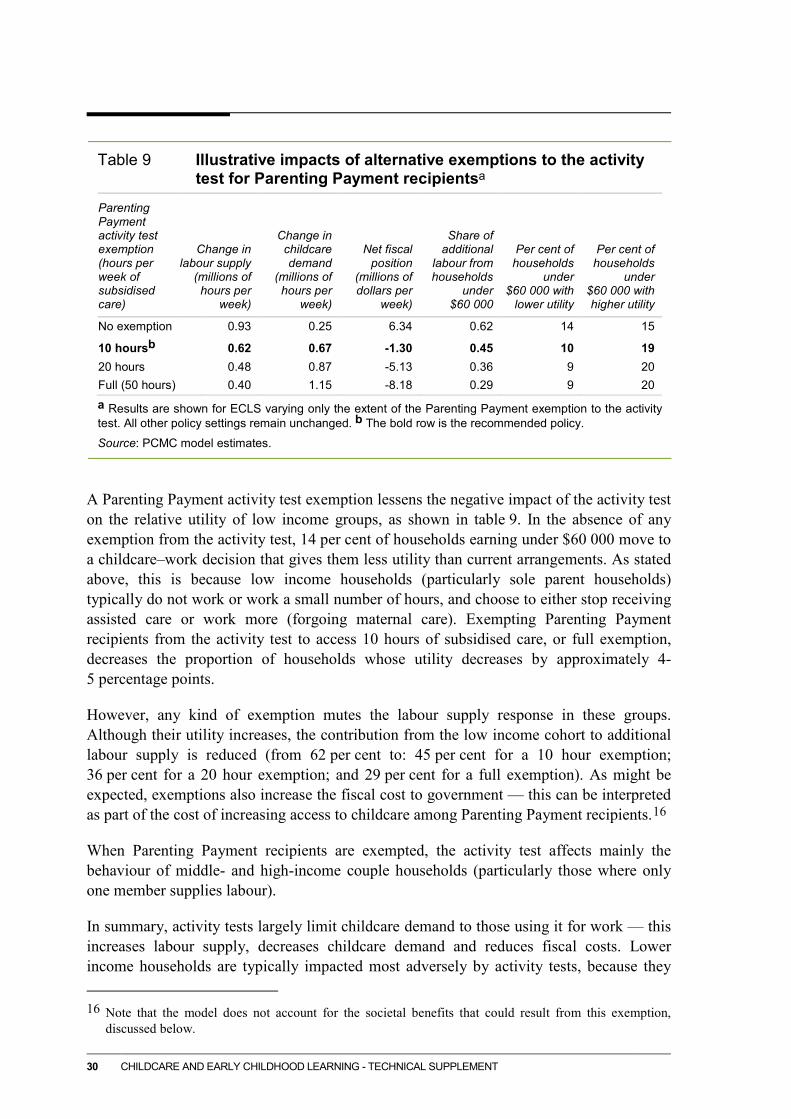
Table 9 Illustrative impacts of alternative exemptions to the activity
test for Parenting Payment recipientsa
Parenting Payment activity test exemption (hours per week of subsidised care)
Change in labour supply
(millions of hours per
week)
Change in childcare demand
(millions of hours per
week)
Net fiscal position
(millions of dollars per
week)
Share of additional
labour from households
under $60 000
Per cent of households
under $60 000 with
lower utility
Per cent of households
under $60 000 with higher utility
No exemption 0.93 0.25 6.34 0.62 14 15
10 hoursb 0.62 0.67 -1.30 0.45 10 19 20 hours 0.48 0.87 -5.13 0.36 9 20 Full (50 hours) 0.40 1.15 -8.18 0.29 9 20
a Results are shown for ECLS varying only the extent of the Parenting Payment exemption to the activity test. All other policy settings remain unchanged. b The bold row is the recommended policy.
Source: PCMC model estimates.
A Parenting Payment activity test exemption lessens the negative impact of the activity test on the relative utility of low income groups, as shown in table 9. In the absence of any exemption from the activity test, 14 per cent of households earning under $60 000 move to a childcare–work decision that gives them less utility than current arrangements. As stated above, this is because low income households (particularly sole parent households) typically do not work or work a small number of hours, and choose to either stop receiving assisted care or work more (forgoing maternal care). Exempting Parenting Payment recipients from the activity test to access 10 hours of subsidised care, or full exemption, decreases the proportion of households whose utility decreases by approximately 4-5 percentage points.
However, any kind of exemption mutes the labour supply response in these groups. Although their utility increases, the contribution from the low income cohort to additional labour supply is reduced (from 62 per cent to: 45 per cent for a 10 hour exemption; 36 per cent for a 20 hour exemption; and 29 per cent for a full exemption). As might be expected, exemptions also increase the fiscal cost to government — this can be interpreted as part of the cost of increasing access to childcare among Parenting Payment recipients.16
When Parenting Payment recipients are exempted, the activity test affects mainly the behaviour of middle- and high-income couple households (particularly those where only one member supplies labour).
In summary, activity tests largely limit childcare demand to those using it for work — this increases labour supply, decreases childcare demand and reduces fiscal costs. Lower income households are typically impacted most adversely by activity tests, because they 16 Note that the model does not account for the societal benefits that could result from this exemption,
discussed below.

MODELLING THE EFFECTS OF CHILDCARE POLICY CHANGES 31
typically work fewer hours, and have greater need for financial assistance to obtain care. Exempting Parenting Payment recipients reduces the negative impact of an activity test on low income households, but also reduces the labour supply gain and increases net fiscal cost.
The model does not take into account the child development benefits of ECEC, and these benefits are not reflected in the metrics showing the impact in the model from the Parenting Payment activity test exemption. There is strong evidence that children facing disadvantage benefit developmentally from early exposure and attendance at high quality ECEC and the additional income generated by parental employment (chapter 5 of the inquiry report).
The results from the 2012 Australian Early Development Index indicate that although children assessed as being developmentally vulnerable when commencing formal schooling are over represented in disadvantaged or lower socioeconomic groups (Department of Education 2013). Children from higher socioeconomic backgrounds who performed poorly in early standardised tests or commenced school with poor development indicators had a tendency to ‘catch up’ academically, whereas similar children from low socioeconomic backgrounds were more likely to remain on a low educational trajectory through school (chapter 5).
Moreover, children from disadvantaged backgrounds are less likely to attend ECEC and preschool in particular than the wider population (chapter 12 of the inquiry report).
Subsidy payments and the benchmark price
A benchmark price arrangement (with the benchmark price set at a value less than the maximum fees observed) to calculate the subsidy introduces the possibility that households facing supply prices below the benchmark price could be eligible for subsidies greater than the fees they face. The recommended policy in the inquiry report caps the payment at 100 per cent of the supply price (‘high’ subsidy rule). However, an alternative was also examined where a households’ rate of assistance is capped at the maximum scheduled rate17 (‘low’ subsidy rule). The impact of both arrangements on the PCMC model results are illustrated in table 10.
17 The ‘scheduled rate’ refers to the rate that the household would receive, paid on the benchmark price, as
opposed to the actual share of the total supply price that is subsidised. For example, a household earning $50 000 would have a scheduled rate of 85 per cent, despite the fact that it’s actual subsidy rate might be higher if the supply price is below the benchmark price.

32 CHILDCARE AND EARLY CHILDHOOD LEARNING - TECHNICAL SUPPLEMENT
Table 10 Illustrative impacts of alternative ‘high’ and ‘low’ subsidy
payment rulesa
Subsidy rule
Change in labour supply
(millions of hours per
week)
Change in childcare demand
(millions of hours per
week)
Net fiscal position
(millions of dollars per
week)
Share of additional
labour from households
under $60 000
Per cent of households
under $60 000 with
lower utility
Per cent of households
under $60 000 with higher utility
High ruleb 0.62 0.67 -1.30 0.45 10 19 Low rule 0.37 -0.15 7.00 0.25 14 14
a Results are shown for ECLS varying only the subsidy payment rule — the ‘high’ rule allows a household to receive a subsidy of up to 100% of the supply price; the ‘low’ rule caps assistance at the maximum scheduled rate. All other policy settings remain unchanged. b The bold row is the recommended policy.
Source: PCMC model estimates.
The low subsidy rule reduces assistance and the incentive to work for many low income households. Low income households (who tend to live in cheaper areas) typically face lower supply price care (potentially below the benchmark price). Receiving the highest rates of assistance under the Commission’s recommended scheme, these households (a) are most likely to hit the 100 per cent assistance cap with the high rule and (b) are (in many cases) eligible for high rates of assistance under current arrangements (upwards of 85 per cent). For many poorer households the low subsidy rule reduces their incentive to work compared to current arrangements. For example, while the 45 per cent of the additional labour supply from the Commission’s recommended scheme comes from households earning under $60 000 initially, they supply only 25 per cent of the increase under a low subsidy rule policy.
The low rule decreases the cost to government. Since a large proportion of childcare used by households earning under $60 000 (approximate 36 per cent of households), and these households receive the highest rates of assistance per hour, capping their subsidies at a low level reduces fiscal cost (saving the government $8.3 million per week relative to the high subsidy rule).
Defining the benchmark price
Alternative definitions of the benchmark price were also examined by the Commission. In the Commission’s recommended policy, the benchmark price is defined as the median price paid for all hours of childcare by type (varying by age for LDC). The Commission explored (a) setting the benchmark price at the 75th percentile of supply prices and (b) calculating subsidies based on actual fees paid (no benchmark price). The impact of these alternative treatments on model results is shown in table 11.
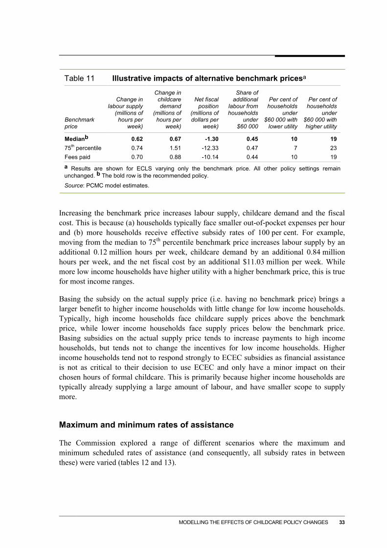
MODELLING THE EFFECTS OF CHILDCARE POLICY CHANGES 33
Table 11 Illustrative impacts of alternative benchmark pricesa
Benchmark price
Change in labour supply
(millions of hours per
week)
Change in childcare demand
(millions of hours per
week)
Net fiscal position
(millions of dollars per
week)
Share of additional
labour from households
under $60 000
Per cent of households
under $60 000 with
lower utility
Per cent of households
under $60 000 with higher utility
Medianb 0.62 0.67 -1.30 0.45 10 19 75th percentile 0.74 1.51 -12.33 0.47 7 23 Fees paid 0.70 0.88 -10.14 0.44 10 19
a Results are shown for ECLS varying only the benchmark price. All other policy settings remain unchanged. b The bold row is the recommended policy.
Source: PCMC model estimates.
Increasing the benchmark price increases labour supply, childcare demand and the fiscal cost. This is because (a) households typically face smaller out-of-pocket expenses per hour and (b) more households receive effective subsidy rates of 100 per cent. For example, moving from the median to 75th percentile benchmark price increases labour supply by an additional 0.12 million hours per week, childcare demand by an additional 0.84 million hours per week, and the net fiscal cost by an additional $11.03 million per week. While more low income households have higher utility with a higher benchmark price, this is true for most income ranges.
Basing the subsidy on the actual supply price (i.e. having no benchmark price) brings a larger benefit to higher income households with little change for low income households. Typically, high income households face childcare supply prices above the benchmark price, while lower income households face supply prices below the benchmark price. Basing subsidies on the actual supply price tends to increase payments to high income households, but tends not to change the incentives for low income households. Higher income households tend not to respond strongly to ECEC subsidies as financial assistance is not as critical to their decision to use ECEC and only have a minor impact on their chosen hours of formal childcare. This is primarily because higher income households are typically already supplying a large amount of labour, and have smaller scope to supply more.
Maximum and minimum rates of assistance
The Commission explored a range of different scenarios where the maximum and minimum scheduled rates of assistance (and consequently, all subsidy rates in between these) were varied (tables 12 and 13).
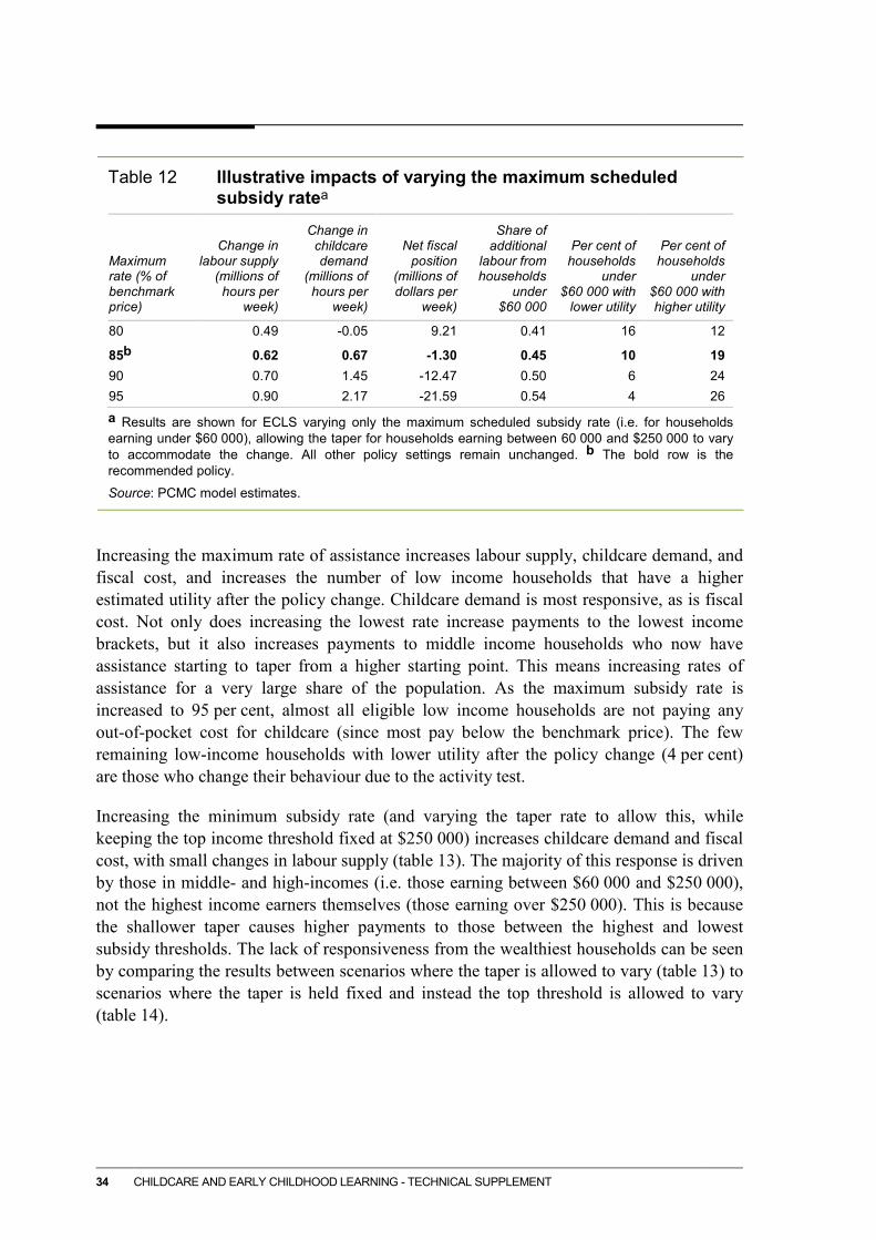
34 CHILDCARE AND EARLY CHILDHOOD LEARNING - TECHNICAL SUPPLEMENT
Table 12 Illustrative impacts of varying the maximum scheduled
subsidy ratea
Maximum rate (% of benchmark price)
Change in labour supply
(millions of hours per
week)
Change in childcare demand
(millions of hours per
week)
Net fiscal position
(millions of dollars per
week)
Share of additional
labour from households
under $60 000
Per cent of households
under $60 000 with
lower utility
Per cent of households
under $60 000 with higher utility
80 0.49 -0.05 9.21 0.41 16 12
85b 0.62 0.67 -1.30 0.45 10 19 90 0.70 1.45 -12.47 0.50 6 24 95 0.90 2.17 -21.59 0.54 4 26
a Results are shown for ECLS varying only the maximum scheduled subsidy rate (i.e. for households earning under $60 000), allowing the taper for households earning between 60 000 and $250 000 to vary to accommodate the change. All other policy settings remain unchanged. b The bold row is the recommended policy.
Source: PCMC model estimates.
Increasing the maximum rate of assistance increases labour supply, childcare demand, and fiscal cost, and increases the number of low income households that have a higher estimated utility after the policy change. Childcare demand is most responsive, as is fiscal cost. Not only does increasing the lowest rate increase payments to the lowest income brackets, but it also increases payments to middle income households who now have assistance starting to taper from a higher starting point. This means increasing rates of assistance for a very large share of the population. As the maximum subsidy rate is increased to 95 per cent, almost all eligible low income households are not paying any out-of-pocket cost for childcare (since most pay below the benchmark price). The few remaining low-income households with lower utility after the policy change (4 per cent) are those who change their behaviour due to the activity test.
Increasing the minimum subsidy rate (and varying the taper rate to allow this, while keeping the top income threshold fixed at $250 000) increases childcare demand and fiscal cost, with small changes in labour supply (table 13). The majority of this response is driven by those in middle- and high-incomes (i.e. those earning between $60 000 and $250 000), not the highest income earners themselves (those earning over $250 000). This is because the shallower taper causes higher payments to those between the highest and lowest subsidy thresholds. The lack of responsiveness from the wealthiest households can be seen by comparing the results between scenarios where the taper is allowed to vary (table 13) to scenarios where the taper is held fixed and instead the top threshold is allowed to vary (table 14).
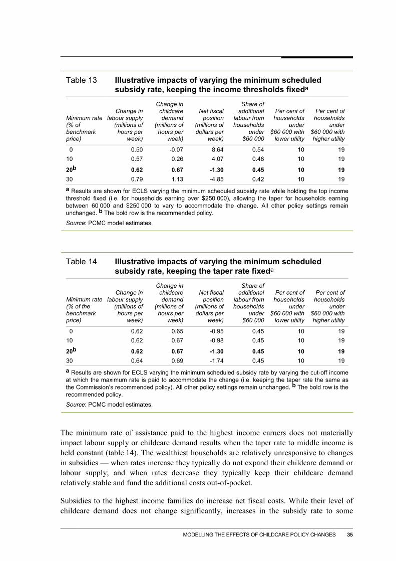
MODELLING THE EFFECTS OF CHILDCARE POLICY CHANGES 35
Table 13 Illustrative impacts of varying the minimum scheduled
subsidy rate, keeping the income thresholds fixeda
Minimum rate (% of benchmark price)
Change in labour supply
(millions of hours per
week)
Change in childcare demand
(millions of hours per
week)
Net fiscal position
(millions of dollars per
week)
Share of additional
labour from households
under $60 000
Per cent of households
under $60 000 with
lower utility
Per cent of households
under $60 000 with higher utility
0 0.50 -0.07 8.64 0.54 10 19 10 0.57 0.26 4.07 0.48 10 19
20b 0.62 0.67 -1.30 0.45 10 19 30 0.79 1.13 -4.85 0.42 10 19
a Results are shown for ECLS varying the minimum scheduled subsidy rate while holding the top income threshold fixed (i.e. for households earning over $250 000), allowing the taper for households earning between 60 000 and $250 000 to vary to accommodate the change. All other policy settings remain unchanged. b The bold row is the recommended policy.
Source: PCMC model estimates.
Table 14 Illustrative impacts of varying the minimum scheduled
subsidy rate, keeping the taper rate fixeda
Minimum rate (% of the benchmark price)
Change in labour supply
(millions of hours per
week)
Change in childcare demand
(millions of hours per
week)
Net fiscal position
(millions of dollars per
week)
Share of additional
labour from households
under $60 000
Per cent of households
under $60 000 with
lower utility
Per cent of households
under $60 000 with higher utility
0 0.62 0.65 -0.95 0.45 10 19 10 0.62 0.67 -0.98 0.45 10 19
20b 0.62 0.67 -1.30 0.45 10 19 30 0.64 0.69 -1.74 0.45 10 19
a Results are shown for ECLS varying the minimum scheduled subsidy rate by varying the cut-off income at which the maximum rate is paid to accommodate the change (i.e. keeping the taper rate the same as the Commission’s recommended policy). All other policy settings remain unchanged. b The bold row is the recommended policy.
Source: PCMC model estimates.
The minimum rate of assistance paid to the highest income earners does not materially impact labour supply or childcare demand results when the taper rate to middle income is held constant (table 14). The wealthiest households are relatively unresponsive to changes in subsidies — when rates increase they typically do not expand their childcare demand or labour supply; and when rates decrease they typically keep their childcare demand relatively stable and fund the additional costs out-of-pocket.
Subsidies to the highest income families do increase net fiscal costs. While their level of childcare demand does not change significantly, increases in the subsidy rate to some

36 CHILDCARE AND EARLY CHILDHOOD LEARNING - TECHNICAL SUPPLEMENT
households in this bracket (where those households have high levels of initial formal childcare demand) result in large additional government payments on pre-existing formal childcare demand. This cost is limited by the fact that very few households (approximately 1.6 per cent) are in the highest income brackets.
It is worth noting that the responses from households in the highest income brackets are the most uncertain of the model results. There are a small number of households in the model (approximately 20) being used to represent population-wide behaviour.

MODELLING THE EFFECTS OF CHILDCARE POLICY CHANGES 37
Appendix A — Data
The Commission’s micro-simulation model uses data from two sources:
– The basic confidential unit record file (CURF) version of the 2011-12 Survey of Income and Housing (SIH) (ABS 2013b). This survey captures key demographic and economic characteristics of individuals residing in private dwellings across Australia.
– An unpublished administrative childcare dataset (Department of Education 2011-12). This dataset provides a comprehensive description of childcare use, childcare prices18, location of services and childcare benefits received.
After considering multiple sources, the basic SIH was adopted as a starting point, since it contained most of the variables necessary for calibrating the model.
Processing the source data
The model’s database includes two samples extracted from the basic SIH — a household sample representing lone parents and a household sample representing coupled parents. When extracting samples, a parent was defined as an adult member of a household who — for the relevant variable — identified as a parent or guardian of a child under 12 years.19
Variables describing parent’s characteristics were extracted from the basic SIH and assigned to the relevant household. Specifically, variables capturing income sources, employment status, number of children, age, occupation, industry of employment, location, educational attainment and hours of childcare use were extracted.
Inconsistent responses
In the basic SIH, several households report inconsistent combinations ‘total current weekly employee income’ and ‘number of hours usually worked per week in main and second jobs’. Specifically, some individuals report no labour income and positive employment, or positive labour income and no employment. If any person in the household reported inconsistent combinations, the household was removed.20 Additionally, any household with no children was removed. In total, 172 households were removed from the model’s database prior to calibration (table A.1).
18 Childcare price was derived by dividing total fees by the number of hours charged for childcare. 19 For a couple with dependent children, it was sufficient for either member of the couple to identify as a
parent or guardian of a child under 12 years. 20 For some households, the primary earner reported working no hours but earning wage income. As these
households were dropped, any work reported by the primary carer would be excluded.
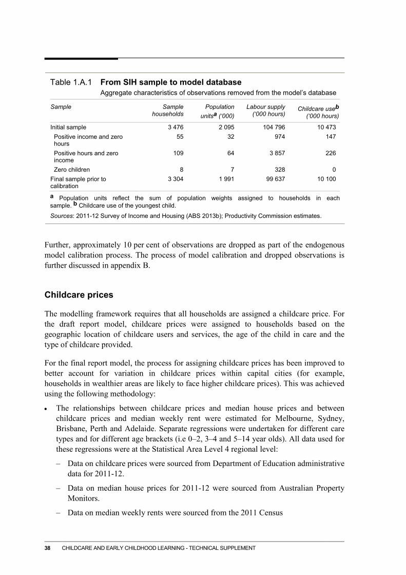
38 CHILDCARE AND EARLY CHILDHOOD LEARNING - TECHNICAL SUPPLEMENT
Table 1.A.1 From SIH sample to model database
Aggregate characteristics of observations removed from the model’s database
Sample Sample households
Population unitsa (‘000)
Labour supply (‘000 hours)
Childcare useb (‘000 hours)
Initial sample 3 476 2 095 104 796 10 473 Positive income and zero hours
55 32 974 147
Positive hours and zero income
109 64 3 857 226
Zero children 8 7 328 0 Final sample prior to calibration
3 304 1 991 99 637 10 100
a Population units reflect the sum of population weights assigned to households in each sample. b Childcare use of the youngest child.
Sources: 2011-12 Survey of Income and Housing (ABS 2013b); Productivity Commission estimates.
Further, approximately 10 per cent of observations are dropped as part of the endogenous model calibration process. The process of model calibration and dropped observations is further discussed in appendix B.
Childcare prices
The modelling framework requires that all households are assigned a childcare price. For the draft report model, childcare prices were assigned to households based on the geographic location of childcare users and services, the age of the child in care and the type of childcare provided.
For the final report model, the process for assigning childcare prices has been improved to better account for variation in childcare prices within capital cities (for example, households in wealthier areas are likely to face higher childcare prices). This was achieved using the following methodology:
• The relationships between childcare prices and median house prices and between childcare prices and median weekly rent were estimated for Melbourne, Sydney, Brisbane, Perth and Adelaide. Separate regressions were undertaken for different care types and for different age brackets (i.e 0–2, 3–4 and 5–14 year olds). All data used for these regressions were at the Statistical Area Level 4 regional level:
– Data on childcare prices were sourced from Department of Education administrative data for 2011-12.
– Data on median house prices for 2011-12 were sourced from Australian Property Monitors.
– Data on median weekly rents were sourced from the 2011 Census

MODELLING THE EFFECTS OF CHILDCARE POLICY CHANGES 39
• Households in the SIH who reside in one of the five aforementioned capital cities were assigned three predicted childcare prices (one each for children aged 0–2, 3–4 and 5–14) based on the value of their house (or their weekly rent if they do not own a house) and the type of care they use. Households who reside in one of the remaining capital cities (Darwin, Canberra or Hobart) or who did not reside in a capital city were assigned the average childcare price of that region based on the 2011–12 administrative data supplied by the Department of Education.
• Nanny prices were calculated by taking the estimated family daycare price and adding $20 (creating a price range of between approximately $25 and $30). This total was then divided by the number of children in a household to obtain a per child per hour cost.
Post simulation calculations
Weighting the SIH
The SIH incorporates population weights for each household. These weights were amended so that the SIH database (after difficult to calibrate observations were dropped, table A.1) reproduced administrative data on the total hours of care used and total ECEC subsidies.
First, population weights in the SIH were adjusted so that the number of hours of care (disaggregated by care type, income level and whether or not the household passed the current CCB activity test) were consistent with Department of Education administrative data for 2013-14. Households that did not used childcare initially were given the average population weight of households that did use childcare initially. These population weights were used to weight the majority of the model outputs.
A set of financial population weights were calculated to weight childcare cost and ECEC subsidy model outputs (after they had been converted to 2013-14 prices). These weights were calculated by adjusting the population weights discussed in the previous section that replicate hours of care, so that the total level of ECEC subsidy (disaggregated by care type, income level and whether or not the household passed the CCB activity test) matched administrative data for 2013-14.
Calculating GDP effects
GDP was calculated by taking the sum of labour incomes and assuming that additional labour supply will be matched by new capital in proportion to the 2013-14 economy-wide average labour–capital ratio. This GDP calculation therefore assumes that there will be:

40 CHILDCARE AND EARLY CHILDHOOD LEARNING - TECHNICAL SUPPLEMENT
• zero unemployment in those people entering the labour market as a result of the policy change, and zero underemployment of those increasing their hours of work in response to the policy change
• zero change in wages and childcare supply prices faced by households within the PCMC model
• no impact on the wages of those households not included in the PCMC model as a result of the modelled labour supply expansion.
Sensitivity analysis
The commission undertook a sensitivity analysis to assess how the model results change when the estimated utility parameters are varied. 1000 Monte Carlo simulations were generated where the utility parameters were assumed vary in a manner consistent with a multinomial normal distribution. The variance-covariance matrix of the multinomial normal distribution was sourced from the multinomial logit estimation process.
None of the other assumptions implicit in the Commission’s modelling framework were varied as part of the sensitivity analysis. These assumptions include that:
• the population weights required to hit the 2013-14 fiscal cost totals contained in the Department of Education administrative data are accurate (as opposed to the SIH population weights, or some combination of the two)
• there were no changes in preferences other than those reflected in variability in the 2011-12 SIH data.

MODELLING THE EFFECTS OF CHILDCARE POLICY CHANGES 41
Appendix B — Model specification
The PCMC model is comprised of three modules:
1. tax and transfer module
2. childcare module
3. decision module.
This appendix presents additional detail on the decision module.
Decision module framework
In the PCMC model, primary care givers have 120 hours in a working week to spend on various activities. It is assumed that 40 of these hours are spent sleeping. Of the remaining 112 hours, primary care givers can choose to work, look after their child(ren), or enjoy leisure, home production or other activities.
Children are also assumed to have 120 hours in the week. They are assumed to sleep for 50 of those hours, and their remaining hours can be spent being minded by the primary care giver, being minded in formal childcare, being minded at school (for school-aged children) or being minded in informal care.
A number of simplifying assumptions are made regarding when these activities can occur.
• If a child is at home and the primary caregiver is at home (and they are both awake), the primary care giver is assumed to care for the child.
• If the child is in formal care (or at school) and the primary care giver is at home, the primary care giver is assumed to undertake leisure/home production.
• If the primary care giver is at work, and the child is not in formal care, the child is assumed to be in informal care (this includes care by the secondary care giver in a couple).
Households are assumed to make two choices simultaneously:
• the number of hours that the primary care giver works
• the number of hours that the youngest child is in formal child care.
Households must choose from a set of discrete options for these two choices:
• labour supply can be 0, 8, 16, 24, 32, 40, 48 or 56 hours a week
• formal child care can be 0, 10, 20, 30, 40 or 50 hours a week.21
21 OSHC care can be 0,4,8,12,16 or 20 hours. This is equal to two fifths of the formal child care choices.

42 CHILDCARE AND EARLY CHILDHOOD LEARNING - TECHNICAL SUPPLEMENT
Households with multiple children are assumed to base labour supply and childcare decisions on the caring needs of the youngest child. That is, childcare for older children mirrors the decision for the youngest child. For example, for a family with one pre-school and one school-age child, if the younger child requires 40 hours per week of non-primary-carer childcare, the older child would also require 40 hours of care (comprising of school and OSHC). The costs associated with the formal care of all children in a household factor in the estimate of a household’s net income and its decisions (that is, households have to pay for and receive utility from care for all children, but the nature of the care decision is driven by the youngest).
Households are permitted to use one type of formal care for children aged 0 to 4 years old. The types of care available for 0 to 4 year olds are: LDC, FDC, qualified nannies, and up to 15 hours per week of preschool. Households who do not use a type of care in the base case, are assigned a childcare type for children aged 0 to 4, based on their income and childcare administrative data to inform the underlying probability distribution. All children aged 5 to 12 years old are assumed to use OSHC if any formal care is required, and receive the same amount of informal care as younger children.
All households are assigned childcare prices using the methodology presented in Appendix A.
The utility function
Households are assumed to choose the combination of the number of hours of work supplied by the primary care giver and the number of hours of formal childcare demanded that maximises household utility.
Primary carers can make a choice from the limited set of discrete combinations of labour and childcare hours mentioned above.
Households derive utility (u) (or disutility) from:
• household income net of taxes and transfers less out-of-pocket childcare costs (y)
• the labour supply of adult members of the household (h)22
• childcare provided by the primary care giver (m)
• childcare provided informally (i).
Like MITTS, the model uses a quadratic utility function. This function consists of squared terms, linear terms for all inputs and cross product terms for all inputs into the utility function.
22 Note that labour supply is also driving the level of income.
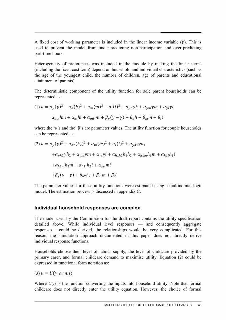
MODELLING THE EFFECTS OF CHILDCARE POLICY CHANGES 43
A fixed cost of working parameter is included in the linear income variable (𝛾). This is used to prevent the model from under-predicting non-participation and over-predicting part-time hours.
Heterogeneity of preferences was included in the module by making the linear terms (including the fixed cost term) depend on household and individual characteristics (such as the age of the youngest child, the number of children, age of parents and educational attainment of parents).
The deterministic component of the utility function for sole parent households can be represented as:
(1) 𝑢 = 𝛼𝑦(𝑦)2 + 𝛼ℎ(ℎ)2 + 𝛼𝑚(𝑚)2 + 𝛼𝑖(𝑖)2 + 𝛼𝑦ℎ𝑦ℎ + 𝛼𝑦𝑚𝑦𝑚 + 𝛼𝑦𝑖𝑦𝑖
𝛼ℎ𝑚ℎ𝑚 + 𝛼ℎ𝑖ℎ𝑖 + 𝛼𝑚𝑖𝑚𝑖 + 𝛽𝑦(𝑦 − 𝛾) + 𝛽ℎℎ + 𝛽𝑚𝑚 + 𝛽𝑖𝑖
where the ‘α’s and the ‘β’s are parameter values. The utility function for couple households can be represented as:
(2) 𝑢 = 𝛼𝑦(𝑦)2 + 𝛼ℎ2(ℎ2)2 + 𝛼𝑚(𝑚)2 + 𝛼𝑖(𝑖)2 + 𝛼𝑦ℎ1𝑦ℎ1
+𝛼𝑦ℎ2𝑦ℎ2 + 𝛼𝑦𝑚𝑦𝑚 + 𝛼𝑦𝑖𝑦𝑖 + 𝛼ℎ1ℎ2ℎ1ℎ2 + 𝛼ℎ1𝑚ℎ1𝑚 + 𝛼ℎ1𝑖ℎ1𝑖
+𝛼ℎ2𝑚ℎ2𝑚 + 𝛼ℎ2𝑖ℎ2𝑖 + 𝛼𝑚𝑖𝑚𝑖
+𝛽𝑦(𝑦 − 𝛾) + 𝛽ℎ2ℎ2 + 𝛽𝑚𝑚 + 𝛽𝑖𝑖
The parameter values for these utility functions were estimated using a multinomial logit model. The estimation process is discussed in appendix C.
Individual household responses are complex
The model used by the Commission for the draft report contains the utility specification detailed above. While individual level responses — and consequently aggregate responses — could be derived, the relationships would be very complicated. For this reason, the simulation approach documented in this paper does not directly derive individual response functions.
Households choose their level of labour supply, the level of childcare provided by the primary carer, and formal childcare demand to maximise utility. Equation (2) could be expressed in functional form notation as:
(3) 𝑢 = 𝑈(𝑦,ℎ,𝑚, 𝑖)
Where U(.) is the function converting the inputs into household utility. Note that formal childcare does not directly enter the utility equation. However, the choice of formal

44 CHILDCARE AND EARLY CHILDHOOD LEARNING - TECHNICAL SUPPLEMENT
childcare (in conjunction with the primary carers labour supply) does determine the use of informal childcare and the use of maternal childcare which are in the utility function.23
This utility function can be re-expressed as a function of only h and f by substituting other functions into (3)24:
• Reflecting constraints on the total available hours of the primary carer, and the total required time of care for children, the amount of care provided by the primary carer (m) and the amount of informal childcare (i) can be thought of as a function C(.) of household labour supply (h) and formal childcare demand (f).
• Similarly, assuming a fixed price of childcare and a fixed wage for each household, household income net of taxes and transfers less childcare costs can be thought of as a function T(.) of the tax and transfer system, household labour supply (h) and formal childcare demand (f).
These substitutions allow the household utility function to be simplified to:
(4) 𝑢 = 𝑈�𝑇(ℎ,𝑓),ℎ,𝑓,𝐶(ℎ,𝑓)� = 𝑉(ℎ,𝑓)
where V(.) is defined for a given wage, childcare price, total hours for the primary carer, total required care for the children, and a given tax and transfer system.
Assuming differentiability, taking the total differential of (4) with respect to h and setting it equal to zero:
(5) 𝑑𝑢𝑑ℎ
= 𝜕𝑉(ℎ,𝑓)𝜕ℎ
+ 𝜕𝑉(ℎ,𝑓)𝜕𝑓
. 𝑑𝑓𝑑ℎ
= 0
Solving equation (5) for h will give the household supply of labour, for given parameters, policy environment and formal childcare demand. A similar relationship can be derived for formal childcare demand as a function of given parameters, policy environment and labour supply, taking the total differential of (4) with respect to f:
(6) 𝑑𝑢𝑑𝑓
= 𝜕𝑉(ℎ,𝑓)𝜕𝑓
+ 𝜕𝑉(ℎ,𝑓)𝜕ℎ
. 𝑑ℎ𝑑𝑓
= 0
These two relationships could be used to derive an individual household’s childcare demand and labour supply as a function of parameters (utility coefficients, wages, childcare prices) and the policy environment (tax, transfer and childcare subsidy system).
23 Informal care is defined as a residual, such that informal childcare equals the minimum of either (a)
formal care less primary-carer labour supply or (b) zero. Informal childcare can be treated as a residual because it is assumed that any formal childcare used by a household will be used while the primary carer is working, unless the formal childcare hours are greater than hours of labour supply. This is consistent with the approach adopted by Gong and Breunig (2012).
24 Note that the model used by the Commission does not substitute out these terms. This substitution is made for illustrative purposes in this section only.
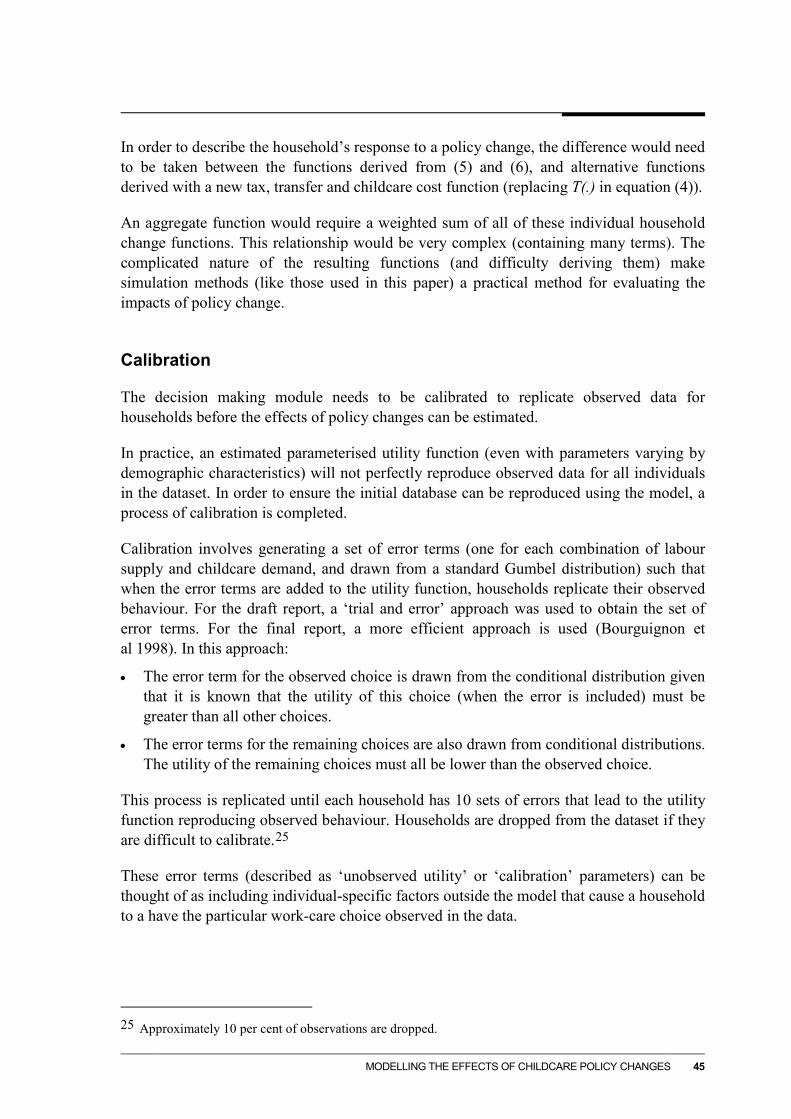
MODELLING THE EFFECTS OF CHILDCARE POLICY CHANGES 45
In order to describe the household’s response to a policy change, the difference would need to be taken between the functions derived from (5) and (6), and alternative functions derived with a new tax, transfer and childcare cost function (replacing T(.) in equation (4)).
An aggregate function would require a weighted sum of all of these individual household change functions. This relationship would be very complex (containing many terms). The complicated nature of the resulting functions (and difficulty deriving them) make simulation methods (like those used in this paper) a practical method for evaluating the impacts of policy change.
Calibration
The decision making module needs to be calibrated to replicate observed data for households before the effects of policy changes can be estimated.
In practice, an estimated parameterised utility function (even with parameters varying by demographic characteristics) will not perfectly reproduce observed data for all individuals in the dataset. In order to ensure the initial database can be reproduced using the model, a process of calibration is completed.
Calibration involves generating a set of error terms (one for each combination of labour supply and childcare demand, and drawn from a standard Gumbel distribution) such that when the error terms are added to the utility function, households replicate their observed behaviour. For the draft report, a ‘trial and error’ approach was used to obtain the set of error terms. For the final report, a more efficient approach is used (Bourguignon et al 1998). In this approach:
• The error term for the observed choice is drawn from the conditional distribution given that it is known that the utility of this choice (when the error is included) must be greater than all other choices.
• The error terms for the remaining choices are also drawn from conditional distributions. The utility of the remaining choices must all be lower than the observed choice.
This process is replicated until each household has 10 sets of errors that lead to the utility function reproducing observed behaviour. Households are dropped from the dataset if they are difficult to calibrate.25
These error terms (described as ‘unobserved utility’ or ‘calibration’ parameters) can be thought of as including individual-specific factors outside the model that cause a household to a have the particular work-care choice observed in the data.
25 Approximately 10 per cent of observations are dropped.

46 CHILDCARE AND EARLY CHILDHOOD LEARNING - TECHNICAL SUPPLEMENT
The wage equation
There is no wage reported in the database for individuals who do not work (and thus do not earn a salary). However, to model the impact of changes in childcare prices, wages are required for all individuals. A wage equation was estimated to provide wages for individuals who do not work initially. Details of this estimation process are presented in appendix C.
MODELLING THE EFFECTS OF CHILDCARE POLICY CHANGES 47
Appendix C — Wage equation and utility function parameter estimation
The Productivity Commission Micro-simulation Childcare (PCMC) model simulates household decisions about labour supply and childcare demand in response to changing childcare subsidies. The decision module within the model controls the manner in which individual households respond to those changing incentives.
Modelling changes in behaviour requires a parameterised household utility function, and the potential wages of those who might choose to enter the labour force. Parameters for behavioural micro-simulation models that consider both labour supply and childcare demand have been estimated by Doiron and Kalb (2005) and Gong and Breunig (2012) — and were used in a preliminary version of the PCMC. However, these papers do not use recent data, and have micro-simulation model specifications that are not identical to the specification adopted by the Commission for the inquiry (appendix B). For these reasons, the Commission estimated new parameters that fit the model and data at hand.
The Commission has followed the econometric approaches documented in Kalb and Scutella (2002), Doiron and Kalb (2005) and Gong and Breunig (2012). This approach involves a two-stage estimation:
• in the first stage, wages for those not participating in the labour market are imputed, based on an equation which corrects for the likelihood of people not participating
• in the second stage, utility parameters are estimated that describe household decisions with respect to labour supply and childcare demand for given wages.
This appendix is divided into three sections. The first section describes the data used for the regressions. The second section describes the wage imputation regression, and the estimated wage equation parameters. The third section details the process of estimating household utility functions, and presents results for the estimated parameters.
C.1 Data description
The data are from the ABS Survey of Income and Housing 2011–12, which is described in appendix A. For the purposes of estimation, the data were split into two broad samples: one for sole parent households; and another for couple households. The data included variables for age, educational attainment, the number of children (and age of youngest child), as well as information on income, hours worked and childcare hours.
The means for some variables of interest are in table C.1. Each observation relates to a coupled or single parent household.

48 CHILDCARE AND EARLY CHILDHOOD LEARNING - TECHNICAL SUPPLEMENT
Table C.1 Mean of key variablesa
Variable Couples Single parents
Age of mother (years) 36.60 36.45 Number of children 1.91 1.80 Youngest child aged 0–2 0.41 0.22 Youngest child aged 3–4 0.15 0.18 Youngest child aged 5–9 0.29 0.34
Youngest child aged 10–14 (omitted)b 0.15 0.26
Work experience 0.74 0.63 Vocational education 0.17 0.24 Degree or higher 0.33 0.15
Diploma or lower education (omitted) b 0.50 0.61
Number of observations 2498 685
a With the exception of ‘age’ and ‘number of children’ all variables are binary – the values represent therefore the proportion of observations that include this characteristic. b Variables are omitted to ensure there is no collinearity. Regressions results should be interpreted as being relative to the omitted category.
Source: Productivity Commission estimates.
C.2 Estimating parameters for an imputed wage equation
Information is required about the financial returns to work (specifically each individual’s wage) in order to model the impact of changes in childcare policies on households decisions — in particular whether a parent will choose to supply (additional) labour as a result of a change to out-of-pocket childcare costs. However, wages are only observed for people who are employed. For this reason, wages have to be imputed for those not currently working.
There is the potential for sample selection bias in those observed to be working, since people are self-selecting into the labour market. To the extent that — for example — people who have higher wages are more likely to choose to work, uncorrected regressions would produce biased wage predictions.
To account for sample selection bias a wage equation was estimated using the approach proposed by Heckman (1979). This involves estimating two equations. First, a ‘selection’ equation estimates the likelihood that a person with a given set of characteristics will self-select into the labour market. Second, a ‘wage’ equation that includes an ‘adjustment factor’ obtained from the selection equation is used to estimate a wage for everybody in the sample, including those not observed to be working.

MODELLING THE EFFECTS OF CHILDCARE POLICY CHANGES 49
The selection equation is estimated as:
𝑃𝑟𝑜𝑏(L = 1 | Z) = Φ(Zγ)
where: L = 1 if employed, 0 otherwise
Z = a vector of explanatory variables
Φ = the cumulative distribution function of the standard normal distribution
γ = parameters to be estimated.
The wage equation is then estimated:
𝑤∗ = X𝛽 + 𝑢
where : w* = a wage, which is only observed if the person is working
The predicted wage, conditional on a person working is:
E[w|X, L = 1] = X𝛽 + E[𝑢|X, L = 1]
where: u = the unobserved determinants of wage offers. Unlike standard ordinary least squares regressions, this is not assumed to be zero.
The above predicted wage equation can be rewritten as:
E[w|X, L = 1] = X𝛽 + 𝜌𝜎uλ(Zγ)
where: ρ = correlation between error terms in the first and second equations
σu = standard deviation of u
λ = inverse mills ratio
Again the predicted wage equation can be expressed as:
E[w|X, L = 1] = X𝛽 + 𝑐λ(Zγ)
where: c = ρσu
When the estimate of c (the coefficient of λ –– the inverse mills ratio) is different from zero a ‘selection effect’ is present. Controlling for the selection effect leads to unbiased estimates in the wage equation for those both with and without jobs in the data. To accurately measure if a selection effect is present, a reliable instrument is needed. An instrument is a variable that affects the likelihood of being employed, but does not affect wages. In practice it can be difficult to find a suitable instrument. The presence of children is often used, and is also used here.

50 CHILDCARE AND EARLY CHILDHOOD LEARNING - TECHNICAL SUPPLEMENT
Results from the estimated wage equation
Coefficient estimates for the selection and wage equations are presented in table C.2.
The inverse mills ratio is statistically significant for partnered women, meaning that there is a positive selection effect for this group.
The presence of children is included in the selection equation, but not the wage equation. This is because it is assumed that having children is likely to have an effect on employment (by potentially decreasing the probability of labour market participation), but not wages. Having children has a negative effect on the likelihood of participating, in particular having a younger child (aged 0–2 years).
Work experience has a positive effect on the probability of employment. Education is also included in the selection equation. As expected, having a degree has a positive effect on employment.
In the wage equation, the coefficient for degree is positive (and statistically significant for partnered women) meaning that a degree (relative to having diploma or lower education) is associated with higher expected wages. Sector and state of residence are also included in the wage equation. Working in the mining sector has the largest positive coefficient.
C.3 Estimating parameters for the utility function
In the behavioural micro-simulation model, household utility is affected by levels of:
• household income including transfers, net of taxes, and net of out-of-pocket costs of childcare
• labour supply (hours worked)
• formal, informal and sole parent/maternal childcare use.
The household utility function is documented in more detail in appendix B.
There are three different types of childcare in the PCMC model: formal childcare, informal childcare and maternal childcare. In the estimation, both informal childcare and maternal childcare enter the utility function. Formal childcare is omitted as including all three forms of childcare would result in an over-specified model.

MODELLING THE EFFECTS OF CHILDCARE POLICY CHANGES 51
Table C.2 Wage equation parameter estimates
Variable Couples, female Single parents
Selection equation Female na -0.78 ** Age -0.15 *** -0.08 *** Age squared/100 0.20 *** 0.09 ** Capital city 0.07 0.14 Number of children 0.01 -0.14 Child aged 0-2 -0.96 *** -0.82 *** Child aged 3-4 -0.36 ** -0.70 *** Child aged 5-9 -0.33 ** -0.32 Work experience 3.94 *** 3.91 *** Vocational education 0.02 -0.26 Degree or higher 0.36 *** 0.30 Wage equation Female na -0.01 Constant 2.00 *** 2.96 *** Age 0.03 * -0.01 Age squared/100 -0.03 0.02 Vocational education 0.05 -0.01 Degree or higher 0.19 *** 0.08 Professional 0.28 *** 0.31 *** Paraprofessional -0.05 0.09 Clerical 0.08 * 0.17 ** Mining 0.69 *** 0.70 ** Manufacturing 0.22 * 0.28 Construction 0.34 ** 0.49 ** Utilities 0.43 ** 0.65 *** Retail/Wholesale 0.02 0.15 Transport 0.07 0.34 Communications 0.34 ** 0.27 Financial business services 0.26 ** 0.25 Other sector 0.18 * 0.25 * South Australia -0.06 0.01 Queensland -0.01 -0.17 ** Victoria -0.06 -0.11 Western Australia -0.04 -0.01 ACT/Northern Territory 0.09 * 0.09 Tasmania -0.09 * -0.06 Capital city 0.08 ** 0.04 Inverse Mills ratio 0.48 *** -0.20 Sigma 0.58 0.45 Rho 0.82 -0.45
*** significant at 1 per cent, ** 5 per cent and * 10 per cent.
Source: Productivity Commission estimates.
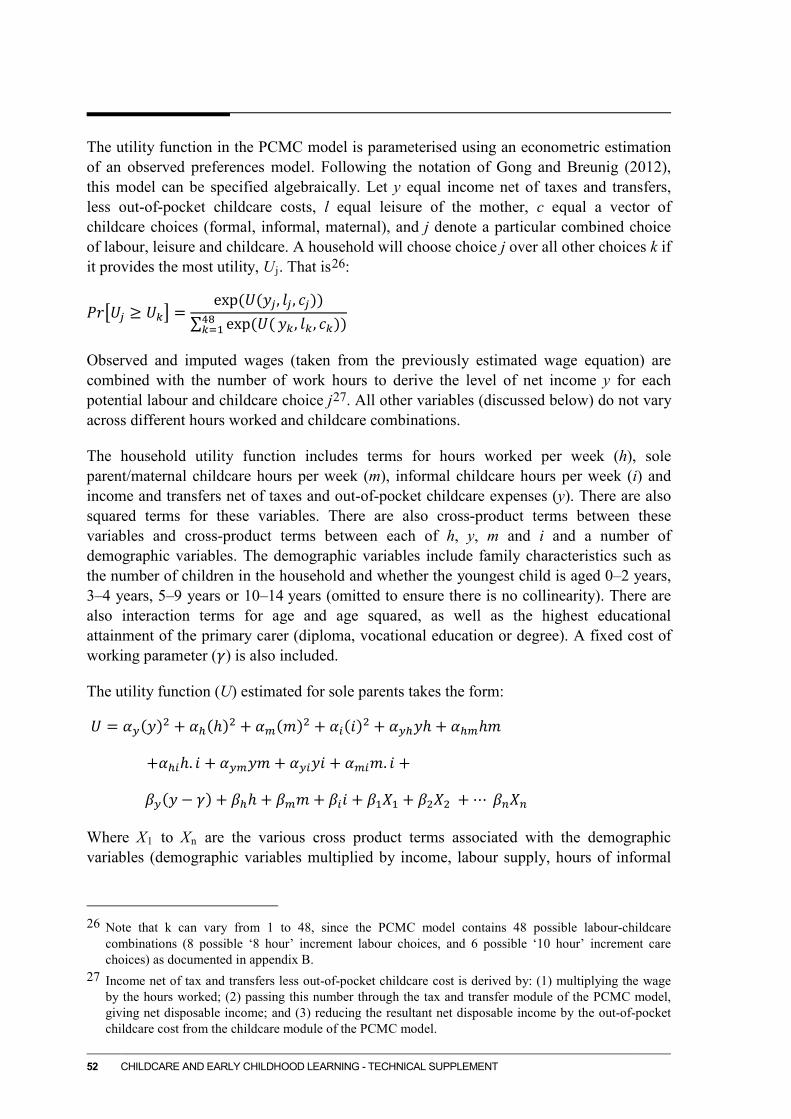
52 CHILDCARE AND EARLY CHILDHOOD LEARNING - TECHNICAL SUPPLEMENT
The utility function in the PCMC model is parameterised using an econometric estimation of an observed preferences model. Following the notation of Gong and Breunig (2012), this model can be specified algebraically. Let y equal income net of taxes and transfers, less out-of-pocket childcare costs, l equal leisure of the mother, c equal a vector of childcare choices (formal, informal, maternal), and j denote a particular combined choice of labour, leisure and childcare. A household will choose choice j over all other choices k if it provides the most utility, Uj. That is26:
𝑃𝑟�𝑈𝑗 ≥ 𝑈𝑘� =exp (𝑈(𝑦𝑗, 𝑙𝑗 , 𝑐𝑗))
∑ exp (𝑈(48𝑘=1 𝑦𝑘, 𝑙𝑘, 𝑐𝑘))
Observed and imputed wages (taken from the previously estimated wage equation) are combined with the number of work hours to derive the level of net income y for each potential labour and childcare choice j27. All other variables (discussed below) do not vary across different hours worked and childcare combinations.
The household utility function includes terms for hours worked per week (h), sole parent/maternal childcare hours per week (m), informal childcare hours per week (i) and income and transfers net of taxes and out-of-pocket childcare expenses (y). There are also squared terms for these variables. There are also cross-product terms between these variables and cross-product terms between each of h, y, m and i and a number of demographic variables. The demographic variables include family characteristics such as the number of children in the household and whether the youngest child is aged 0–2 years, 3–4 years, 5–9 years or 10–14 years (omitted to ensure there is no collinearity). There are also interaction terms for age and age squared, as well as the highest educational attainment of the primary carer (diploma, vocational education or degree). A fixed cost of working parameter (𝛾) is also included.
The utility function (U) estimated for sole parents takes the form:
𝑈 = 𝛼𝑦(𝑦)2 + 𝛼ℎ(ℎ)2 + 𝛼𝑚(𝑚)2 + 𝛼𝑖(𝑖)2 + 𝛼𝑦ℎ𝑦ℎ + 𝛼ℎ𝑚ℎ𝑚
+𝛼ℎ𝑖ℎ. 𝑖 + 𝛼𝑦𝑚𝑦𝑚 + 𝛼𝑦𝑖𝑦𝑖 + 𝛼𝑚𝑖𝑚. 𝑖 +
𝛽𝑦(𝑦 − 𝛾) + 𝛽ℎℎ + 𝛽𝑚𝑚 + 𝛽𝑖𝑖 + 𝛽1𝑋1 + 𝛽2𝑋2 + ⋯ 𝛽𝑛𝑋𝑛
Where X1 to Xn are the various cross product terms associated with the demographic variables (demographic variables multiplied by income, labour supply, hours of informal
26 Note that k can vary from 1 to 48, since the PCMC model contains 48 possible labour-childcare
combinations (8 possible ‘8 hour’ increment labour choices, and 6 possible ‘10 hour’ increment care choices) as documented in appendix B.
27 Income net of tax and transfers less out-of-pocket childcare cost is derived by: (1) multiplying the wage by the hours worked; (2) passing this number through the tax and transfer module of the PCMC model, giving net disposable income; and (3) reducing the resultant net disposable income by the out-of-pocket childcare cost from the childcare module of the PCMC model.

MODELLING THE EFFECTS OF CHILDCARE POLICY CHANGES 53
childcare, and hours of sole parent/maternal childcare). For couples, there are additional cross product terms for the husband.
Table C.3 lists all utility function variables used.
Table C.3 Variables included in the utility function regressions
Variable Couples Single parents
Income, linear and squared Yes Yes Labour supply, linear and squared Yes Yes Maternal childcare, linear and squared Yes Yes Informal childcare, linear and squared Yes Yes Income × Hours worked by husband Yes No Labour supply × Income Yes Yes Labour supply × Hours worked by husband Yes No Maternal childcare × Hours worked by husband Yes No Labour supply × maternal childcare Yes Yes Income × maternal childcare Yes Yes Informal childcare × hours worked by husband Yes No Labour supply × Informal childcare Yes Yes Income × informal childcare Yes Yes Maternal childcare × informal childcare Yes Yes Other cross product terms: Income, labour supply, maternal childcare, informal childcare ×
Youngest child aged 0–2 Yes Yes Youngest child aged 3–4 Yes Yes Youngest child aged 5–9 Yes Yes Number of children Yes Yes Age of woman, squared Yes Yes Vocational education woman Yes Yes Diploma woman Yes Yes Degree woman Yes Yes Female No Yes
Fixed cost of working Yes Yes × female No Yes
A multinomial logit model is used because the dependent variable is a discrete choice outcome (1 of 48 possible discrete labour-childcare choice combinations), and the utility term is an unobserved variable. (See appendix B for a more detailed description of the choices available to households in the model.)
Results from the estimation of the utility function
The estimated parameters for the utility function are presented in table C.4.
54 CHILDCARE AND EARLY CHILDHOOD LEARNING - TECHNICAL SUPPLEMENT
The estimated linear term for income is positive, and the squared term parameter estimate is negative (these coefficients are significant for females with partners), consistent with decreasing marginal utility.
Table C.4 Utility function parameter estimates
Variable Couples Single parents
Income squared × 100 000 -0.05 *** -0.02 Labour supply squared × 100 -0.24 *** -0.24 ** Maternal childcare squared × 100 0.03 -0.06 Informal childcare squared × 100 0.17 *** 0.09 Income × Hours worked by husband 10 000 0.08 na Labour supply × Income × 100 000 0.03 -6.20 Labour supply × Hours worked by husband × 100 0.03 na Maternal childcare × Hours worked by husband × 100 0.04 na Labour supply × maternal childcare × 100 -0.26 *** -0.59 *** Income × maternal childcare × 10 000 0.07 2.26 *** Informal childcare × hours worked by husband × 100 0.01 na Labour supply × Informal childcare × 100 0.58 *** 1.29 *** Income × informal childcare × 10 000 -0.14 *** -0.14 Maternal childcare × informal childcare × 100 0.83 *** 1.29 *** Income 0.02 *** 0.005
Youngest child aged 0–2 × 100 0.10 * 0.40 Youngest child aged 3–4 × 100 0.09 0.15 Youngest child aged 5–9 × 100 -0.02 0.13 Number of children × 100 -0.02 -0.03 Age of woman × 100 -0.07 *** 0.03 Age of woman squared × 10 000 0.10 *** -0.03 Vocational education woman × 100 -0.24 *** 0.08 Diploma woman × 100 -0.22 *** -0.31 Degree woman × 100 -0.19 *** -0.54 *** Female × 100 na -0.58 **
Labour supply -0.12 0.38 ** Youngest child aged 0–2 × 100 -0.60 -8.79 *** Youngest child aged 3–4 × 100 1.87 -4.38 Youngest child aged 5–9 × 100 -1.44 -1.88 Number of children × 100 -0.04 0.47 Age of woman × 100 1.87 *** 0.24 Age of woman squared × 10 000 -2.67 *** -0.67 Vocational education woman × 100 4.19 *** -0.41 Diploma woman × 100 3.91 *** 1.75 Degree woman × 100 4.07 *** 5.75 ** Female × 100 na -2.06
(continued next page…)

MODELLING THE EFFECTS OF CHILDCARE POLICY CHANGES 55
Table C.4 (continued)
Variable Couples Single parents
Maternal childcare 0.52 *** 0.56 *** Youngest child aged 0–2 -0.54 *** -0.45 *** Youngest child aged 3–4 -0.53 *** -0.44 *** Youngest child aged 5–9 -0.27 *** -0.20 *** Number of children × 100 1.18 *** -2.72 Age of woman × 100 0.40 -0.08 Age of woman squared × 10 000 -0.59 -0.03 Vocational education woman × 100 1.29 -3.04 * Diploma woman × 100 0.01 -5.77 *** Degree woman × 10 000 -0.16 -5.73 *** Female × 100 na -0.37
Informal childcare 0.02 -0.68 *** Youngest child aged 0–2 -0.53 *** -0.32 *** Youngest child aged 3–4 -0.54 *** -0.34 *** Youngest child aged 5–9 -0.26 *** -0.18 *** Number of children × 100 0.98 *** 1.63 ** Age of woman × 100 -0.44 -0.32 Age of woman squared × 10 000 0.56 0.53
Fixed cost of working -1.86 *** -4.88 *** Female na 1.86 ***
*** significant at 1 per cent, ** 5 per cent and * 10 per cent.
Source: Productivity Commission estimates.
Labour supply could be expected to have a positive or negative effect on utility: increasing hours worked can be a source of utility for those who enjoy work, but it reduces the amount of time spent on leisure or caring for children. In the model, the linear term for labour supply is negative for females with partners, but positive (and statistically significant) for single parents. The squared term parameter estimate for labour supply is negative for both couples and sole parents.
Households also derive utility from spending time with children and from informal childcare (for example, children spending time with grandparents or with the partner in partnered households). The results include a positive parameter estimate for the linear maternal childcare term for couples and sole parents. The squared term parameter estimate is positive for couples and negative for sole parents. For informal childcare, the linear term is close to zero for couples and negative (and statistically significant) for sole parents. Quadratic terms for informal childcare are positive for both couples and sole parents.
The many interaction terms account for the potential diversity in effects across different demographic groups.
56 CHILDCARE AND EARLY CHILDHOOD LEARNING - TECHNICAL SUPPLEMENT
Appendix D — Workshop and referee’s report
In accordance with the Productivity Commission Act 1998 (Cwlth), the Commission appointed as referee Professor Guyonne Kalb, Director of the Labour Economics and Social Policy Program at the Melbourne Institute (University of Melbourne) and conducted a workshop on 6 August 2014 for the purpose of reporting on the modelling. A list of participants at the Commission’s modelling workshop is presented in appendix A of the inquiry report.
Comments from Professor Guyonne Kalb
Overall the technical paper is easy to read, and provides good intuition behind some of the anticipated effects, which is useful for understanding the impact of the proposed policy change.
Simulation results by subgroups
Detailing the differential impacts that the policy may have on different groups of families is an important feature of this paper. Grouping families by whether they use formal childcare and whether the primary carer supplies labour in the base case provides useful insights. However, I would suggest an additional separate set of results by whether the family is a single-parent family or a two-parent family. Given the different circumstances of single parents compared to couples with children, and the importance of supporting single-parent families particularly with regard to labour force participation, it would be important to assess the effects of a policy change on each group separately.
The number of separate models, two vs four
I agree with the authors of the report that estimating separate models for single parents and couple families is essential. However, I would probably not further divide these two groups in a subgroup with a youngest child of pre-school age and a subgroup with a youngest child of school age. Especially, since this would only be feasible for couple families, given the small sample size of single parents, whereas the distinction is probably more important for single parents who do not have a “back-up” carer at home.
Using parameters from previous studies vs estimation
I also agree with the authors that the simulation results presented here are preliminary, and need to be redone after estimating the suggested model on recent data. Should this not be feasible within the time available, then I suggest to check the appropriateness of the current parameter values by carrying out a simulation without calibrating to the observed labour supply and formal childcare demand. This would allow you to compute the expected

MODELLING THE EFFECTS OF CHILDCARE POLICY CHANGES 57
proportions working at each of the discretised hours points and using each of the discretised hours of formal childcare. The expected proportions could then be compared to the actual observed proportions at each hours point. If these proportions are reasonably similar, it would suggest that the chosen parameters are a reasonable fit to the observed data. I am making this suggestion, because I am not sure that the sensitivity testing is enough. I may misunderstand what is done, but it seems as if all parameters are just increased/decreased across the board by a certain percentage, whereas the key issue may be how the parameters relate to each other.
When using parameters from previous studies, additional information on where each parameter has come from would be useful. Perhaps a few notes could be added to the tables presented in Appendix C to indicate where each coefficient has come from.
Model specification
I do like the way in which the model is specified, allowing labour supply by the primary carer (h), net household income (y), formal care (f) and care by the primary carer (m) to influence the household’s utility. However, there is an inconsistency between the model specification and how it is described. On p.6 the paper states “Households derive utility from caring for children directly” and on p.34 the utility function in equations 1, 2 and 3 includes m (childcare provided by the primary care giver). From these functions, the authors go on to derive a utility function just depending on hours of work and formal childcare demand. They argue that m is still part of this, but is substituted out by replacing m by a function of h and f. However this does not take into account the informal care that may be used by the family, and so h and f are not sufficient to determine m. Therefore the resulting model does not implicitly take into account the utility of m, but is just based on the utility derived from net income, labour supply and formal childcare. There is no way to distinguish m from informal care; both types of care would be equally valued.
Informal care and m can only be distinguished if we observe how many hours of either informal care or m are used. Is this observed in SIH? I am assuming the answer is yes, given that ‘primary carer childcare’ terms are included in the tables in Appendix C. To enable estimation of such terms using recent data, the choice for primary carer childcare hours needs to be endogenous in the model. That is in addition to choosing labour supply and formal childcare hours, the hours of childcare by the primary carer also need to be chosen.
The utility functions presented in equations 1 and 2 are not quite complete as some linear, quadratic and interaction terms are missing from both equations, whereas in equation 2, the terms including h1 should be left out since hours of the primary earner are assumed to be exogenous. However, h1 could enter preference parameters β as an explanatory variable influencing the hours worked by the primary carer and the demand for formal childcare. The income earned from labour supply by the primary earner would enter y as other household income.
Before estimating the specified models, the utility functions need to be properly defined.

58 CHILDCARE AND EARLY CHILDHOOD LEARNING - TECHNICAL SUPPLEMENT
References
ABS (Australian Bureau of Statistics) 2013a, Information Paper: Survey of Income and Housing, User Guide, Australia, August, Cat. no. 6553.0, Canberra.
—— 2013b, Microdata: Income and Housing, Australia, 2011-12, http://www.abs.gov.au /AUSSTATS/[email protected]/Lookup/6541.0.30.001Main+Features12011-12?OpenDocument (accessed 26 June 2014).
Bourguignon, F., Fournier, M. and Gurgand, M. 1998, Distribution, Development and Education: Taiwan, 1979-1994, http://ssrn.com/abstract=587202 orhttp://dx.doi.org /10.2139/ssrn.587202.
Breunig, R. and Gong, X. 2011, Estimating net child care price elasticities of partnered women with pre-school children using a discrete structural labour supply-child care model, Discussion Paper, Centre for Economic Policy Research.
——, —— and King, A. 2010, How responsive is female labour supply to child care costs - new Australian estimates, Working Paper, The Treasury.
Creedy, J., Duncan, A., Kalb, G., Kew, H. and Scutella, R. 2004, The Melbourne Institute Tax and Transfer Simulator (MITTS), The Melbourne Institute of Applied Economic and Social Research.
Creedy, J. and Kalb, G. 2005, Discrete Hours Labour Supply Modelling: Specification, Estimation and Simulation. Journal of Economic Surveys, 19(5), 697–734.
Creedy, J. and Kalb, G. 2006, Labour Supply and Micro-simulation: The Evaluation of Tax Policy Reforms, Cheltenham: Edward Elgar.
Doiron, D. and Kalb, G. 2005, Demands for childcare and household labour supply in Australia, Economic Record, vol. 81, 215–236.
Gong, X. and Breunig, R. 2012, Estimating Net Child Care Price Elasticities of Partnered Women with Pre-school Children Using a Discrete Structural Labour Supply-Child Care Model, November, Working Paper, Australian Treasury, Canberra.
Heckman, J. 1979, ‘Sample Selection Bias as a Specification Error’, Econometrica, vol. 47, no. 1, pp. 153–61.
Household, Income and Labour Dynamics in Australia (HILDA) 2013, 2013 Annual Report.
Kalb, G. and Scutella, R. 2002, Estimation of Wage Equations in Australia: Allowing for Censored Observations of Labour Supply, May, Working Paper No. 8/02, Melbourne Institute.
Summerfield, M., Freidin, S., Hahn, M., Ittak, P., Li, N., Macalalad, N., Watson, N., Wilkins, R. and Wooden, M. 2014, HILDA User Manual, Release 12 June, The Melbourne Institute of Applied Economic and Social Research.