Modelling and simulation of laser chemical processing (LCP ...
167
MODELLING AND SIMULATION OF LASER CHEMICAL PROCESSING (LCP) FOR THE MANUFACTURING OF SILICON SOLAR CELLS DISSERTATION zur Erlangung des akademischen Grades des Doktors der Naturwissenschaften (Dr. rer. nat.) an der Universität Konstanz Fachbereich Physik vorgelegt von Andreas Fell Fraunhofer Institut für Solare Energiesysteme Freiburg im Breisgau 2010
Transcript of Modelling and simulation of laser chemical processing (LCP ...

i
MODELLING AND SIMULATION OF LASER CHEMICAL PROCESSING (LCP) FOR THE
MANUFACTURING OF SILICON SOLAR CELLS
DISSERTATION
zur Erlangung des akademischen Grades des Doktors der Naturwissenschaften
(Dr. rer. nat.)
an der Universität Konstanz Fachbereich Physik
vorgelegt von
Andreas Fell
Fraunhofer Institut für Solare Energiesysteme Freiburg im Breisgau
2010

i
Table of contents
Table of contents........................................................................................................................i
1 Introduction .......................................................................................................................1
1.1 Motivation ..................................................................................................................1
1.2 LCP – status of research .............................................................................................3
1.3 Literature review ........................................................................................................7
1.4 Aims and scopes .........................................................................................................7
2 Mathematical modelling ...................................................................................................9
2.1 Overview of physical effects in LCP..........................................................................9
2.2 Optics........................................................................................................................11
2.2.1 Complex refraction index of silicon .....................................................................12
2.2.2 Absorption ............................................................................................................13
2.2.3 Reflection .............................................................................................................15
2.3 Thermodynamics ......................................................................................................19
2.3.1 Heat transport .......................................................................................................19
2.3.2 Phase change solid – liquid ..................................................................................21
2.3.3 Evaporation...........................................................................................................23
2.3.4 Species transport...................................................................................................25
2.4 Fluid dynamics .........................................................................................................27
2.4.1 Basic fluid flow ....................................................................................................28
2.4.2 Multiphase flow....................................................................................................28
2.4.3 Melting and solidification.....................................................................................29
2.5 Chemistry .................................................................................................................30
2.5.1 Photochemical radical generation.........................................................................30
2.5.2 Reactions ..............................................................................................................31
3 Fundamentals of the simulation methods .....................................................................32
3.1 PDE solving by finite differences.............................................................................32
TABLE OF CONTENTS
ii
3.1.1 Spatial discretization............................................................................................ 33
3.1.2 Time integration................................................................................................... 36
3.1.3 Alternating direction explicit (ADE) method ...................................................... 38
3.2 Fluent ....................................................................................................................... 39
3.2.1 Solver basics ........................................................................................................ 40
3.2.2 User defined code – UDS and UDF..................................................................... 41
3.2.3 Multiphase flow ................................................................................................... 42
4 Implementation............................................................................................................... 43
4.1 Heating and radical generation in the liquid jet ....................................................... 43
4.2 LCPSim: optics and thermodynamics at the reaction spot ...................................... 47
4.2.1 Solving of the heat transport equation ................................................................. 48
4.2.2 Implementation of the ADE method.................................................................... 51
4.2.3 Treatment of the surface geometry ...................................................................... 55
4.2.4 Intensity distribution, surface reflections and raytracing..................................... 56
4.2.5 Semi analytical heat sources ................................................................................ 61
4.2.6 Surface recession due to evaporation................................................................... 61
4.2.7 Diffusion of impurity atoms in silicon melt......................................................... 64
4.2.8 Multilayer implementation................................................................................... 66
4.2.9 Grid generation and adaptation ............................................................................ 67
4.2.10 User settings and program structure................................................................. 71
4.2.11 Verification ...................................................................................................... 73
4.3 Adaption of Fluent ................................................................................................... 78
4.3.1 Separate temperature fields.................................................................................. 78
4.3.2 Melting / solidification and density change ......................................................... 79
4.3.3 Free surface heat transfer ..................................................................................... 81
4.3.4 Verification .......................................................................................................... 83
4.4 Coupling of LCPSim and Fluent.............................................................................. 87
4.4.1 Coupling algorithm .............................................................................................. 88

TABLE OF CONTENTS
iii
4.4.2 Verification...........................................................................................................90
5 Simulation results............................................................................................................92
5.1 Heating and radical generation in the liquid jet........................................................92
5.2 Influence of basic parameters in silicon laser processing.........................................95
5.3 Dry laser ablation......................................................................................................99
5.3.1 Silicon...................................................................................................................99
5.3.2 Silicon nitride layer ............................................................................................101
5.4 Ablation of silicon by LCP.....................................................................................102
5.4.1 Evaporation.........................................................................................................102
5.4.2 Melt expulsion by the liquid jet..........................................................................104
5.4.3 Cooling effect .....................................................................................................109
5.5 Dry laser doping .....................................................................................................111
5.6 LCP doping.............................................................................................................112
5.6.1 Simulations with flat top profile.........................................................................113
5.6.2 Influence of inhomogeneous intensity profile ....................................................115
6 Summary........................................................................................................................122
7 Deutschsprachige Zusammenfassung..........................................................................127
A Program code and settings ...........................................................................................132
A.1 LCPSim: start.m .....................................................................................................132
A.2 LCPSim: gridadapt_2d.m .......................................................................................135
A.3 LCPSim: ade_2d.m.................................................................................................139
A.4 LCPSim: sims.m.....................................................................................................142
A.5 Fluent: Fluent C-code for UDFs.............................................................................143
A.6 Fluent: solver settings.............................................................................................147
B List of symbols and abbreviations ...............................................................................149
C Publications....................................................................................................................156
References .............................................................................................................................158
Danksagung...........................................................................................................................161


1
1 Introduction
1.1 Motivation
A major part of the current threats to the human civilisation originates from the world energy system, which is based mainly on fossil fuels. On the one hand, the limited amount of fossil and nuclear resources will lead to a dramatic increase of energy cost in the mid term, the effects of which are already clearly visible, which will have an unforeseeably great impact on world poverty and social stability. On the other hand, the air pollution by burning fossil fuels affects seriously the world’s flora and fauna, mainly due to climate change by the greenhouse effect. The greenhouse gases emitted up to now are already high enough to possibly heat up the world’s average temperature by over 2 degrees, which is treated as a critical value for non-healable climate change [1] with strongly increased weather extremes, dessert spreading, sea-level rise and so on.
Therefore one of the biggest tasks for mankind is to strongly reduce and finally completely eliminate the amount of fossils and nuclear power as primary energy in a very fast way. Besides energy savings the highest effort has to be made to develop cost efficient renewable energy usage, because only then is a rapid worldwide market introduction possible. The example of Germany showed that with a suitable political frameset, namely the EEG [2], extremely high growth rates of installed renewable power capacities can be achieved. This strong market growth at the same time increases research and development efforts, which leads to a decreasing cost of the installations. For wind power, grid parity has already been reached, even in moderately windy regions. This is now the reason for its worldwide rapid market growth even without high political support and there will be a significant contribution to world energy production in the near future.
Another promising renewable energy source is photovoltaics. The potential of usable solar radiation on earth is much greater than world energy consumption. Also, photovoltaics have shown rapid growth rates of %50 since 2003 [3], as shown in Fig. 1-1. Currently, grid parity
has only been reached in very sunny regions. Therefore political support is still needed to ensure further cost reductions. In addition to cost reductions by large scale manufacturing, an important key is to introduce new technologies to increase the light conversion efficiency of a solar cell, which directly improves the cost per WattPeak ratio of the final power plant.

INTRODUCTION
2
Fig. 1-1: World PV module production from 1990 to 2007 taken from [3]
This work was done in the field of crystalline silicon solar cells, which have the biggest market share, because of technology transfer from semiconductor industry and the higher efficiency compared to thin film technologies. It is quite well known, how to manufacture a highly efficient crystalline silicon solar cell, for example the PERC cell [4] or the back-contact cell [5]. But a great deal of necessary manufacturing steps, mainly consisting of photolithography, are too cost intensive for an industrial application. Thus world research activities in this field currently focus on the development of new cheap processes to introduce high efficiency cell structures in industry.
Within this scope lasers offer a variety of new promising applications. They work maskless, contact-free and are able to process arbitrary geometries with very high speed. A special laser application, called laser chemical processing (LCP), is currently being developed at Fraunhofer ISE. Here a laser and a liquid jet containing suitable chemicals are combined to trigger different thermochemical processes at the reaction spot. With this technique, it is for example possible to create local phosphorous doping underneath the front metal contact fingers in just one process step, which can significantly increase the efficiency of the solar cell.
This work contributes to the development of LCP by gaining an understanding of the process physics. The use of simulations enables a better interpretation of experimental results leading to more efficient selection of parameters and optimization.

INTRODUCTION
3
1.2 LCP – status of research
Fig. 1-2: Sketch of the LCP principle
LCP is based on the LaserMicroJet™ (LMJ) technology by Synova S.A. and was developed by Richerzhagen in 1994 [6, 7]. A hair thin jet is generated by pumping water through a tiny sharp edged nozzle. Applying the correct pressures on the order of 100 bar, a constricted jet is formed, which is stable up to 1000 times the nozzle diameter and can in this way act as an optical waveguide. LMJ is mainly used for the cutting of different materials with pulsed or continuous wave (CW) high power lasers. The laser heats, melts and evaporates the work piece and the high velocity liquid jet carries away the ablated material.
LCP was introduced by Willeke and Kray [8, 9] by replacing water with solvents containing suitable chemicals, which enables a variety of combined thermal, hydrodynamic and chemical processes at the reaction spot. Since 2003 the Fraunhofer Institute for Solar Energy Systems (ISE) is the only institution developing different LCP applications for the manufacturing of crystalline silicon solar cells. Possible applications range from microstructuring, for example the opening of passivation layers or edge isolation, to wafering, which aims to cut wafers from an ingot, to local doping and metallization, which enables selective emitter and local back surface field (LBSF) formation. Two examples, the wafering and the local doping, will be discussed in the following.
Wafering
Wafering is the process of cutting wafers out of a crystalline silicon ingot. This is usually done by a multi wire slurry saw (MWSS), where thousands of parallel wires abrasively cut an
laser beam
focusing lens
nozzle hole
window
pressure chamber
liquid jet
reaction spot
processed region

INTRODUCTION
4
ingot. The MWSS is able to produce wafers with a thickness down to 150 µm, having a kerf loss of at least the same amount. The surface of the wafers is highly damaged and contaminated especially by metals from the wire. Therefore wet chemical etching and cleaning steps are needed afterwards which further increases the overall loss of silicon. This loss is very critical considering the high price of crystalline silicon.
Because in LCP the laser is focused over the whole stable jet length in the centimetre range, very deep grooves with high aspect ratios can be processed. This makes it suitable for a wafering application. Advantages in regard to the MWSS are the potential of smaller kerfs and a better surface quality, which in overall reduces the loss of silicon significantly and makes additional etching and cleaning unnecessary. LCP wafering also has the potential of silicon recycling by using suitable reactants, namely chlorine, which would further reduce the loss of silicon.
The research in this field is focused on searching for suitable laser parameters and chemical additives to achieve deep cuts with good surface quality. Progress has been published by Hopman, Mayer and Fell [10, 11]. The ability of 7 cm cutting depth has been proven and the ablation efficiency and ablation mechanism of different laser systems has been discussed in detail. Chlorine is shown to have a very high etch rate on molten and evaporated silicon but shows no etching on solid silicon, which makes it suitable to support the thermal ablation. More recently, Mayer [12] proved a positive influence on cut quality and groove shape by adding chlorine to Fluorinert FC-770 as a solvent, see Fig. 1-3. Wafering with LCP is still in the stage of fundamental research, therefore increasing understanding of the process is necessary for further development. For this the simulation results of the present work contribute to the understanding of different ablation mechanisms like evaporation and melt expulsion.
Fig. 1-3: Influence of chlorine in the liquid jet on the groove shape after LCP line scans; left: low chlorine concentration; right: High chlorine concentration [12]
little Cl much Cl

INTRODUCTION
5
Doping
Doping with LCP is already close to an industrial application. Most relevant is the selective emitter formation on p-type solar cells. For high efficiency, a lowly doped emitter with a high “blue response” is needed. But a high surface doping is needed to ensure a good contact resistance to the metal contacts. The selective emitter combines these two issues by having a lowly doped emitter and local high doping underneath the front metal contact fingers. The high doping also reduces recombination losses in the contact area, which means neutralization of electrons and holes. Therefore the high doping increases the overall efficiency significantly and cheap processes for the manufacturing of selective emitters are of great industrial interest.
Fig. 1-4: High efficiency p-type silicon solar cell structure (PERC) with selective emitter and local back surface field (LBSF)
Usually selective emitters are produced by photolithography with a lot of masking and etching steps, which is much too cost intensive for an industrial application. With LCP, a technique is proposed that can achieve local high doping in a fast single step. For n-doping, phosphoric acid is used as a liquid medium which acts as a phosphorus dopant source. The laser power melts the silicon at the reaction spot, the phosphorus is thermally atomized and it then diffuses into the silicon melt. Because the phosphorus diffusion coefficient in the silicon melt is several orders of magnitude higher than in solid silicon, precise local doping in very short melt times is possible. Pulsed lasers with pulse durations down to a few nanoseconds are sufficient to create appropriate doping. Advantages to dry laser doping processes are the nearly infinite doping source which does not have to be placed in an extra step and enables grooving and doping at the same time. A disadvantage is that melt flow by the liquid jet can
p doped base
front metal contact passivation and antireflection layer
n-doped emitter
rear metal contact
passivation layer
local high p doping
local high n doping

INTRODUCTION
6
create a bad crystal quality, whereas in dry laser doping with low power, the melt resolidificates without much movement.
Solar cell results with LCP doping have been published in [13] and [14], where it is shown that with low power nanosecond laser pulses a proper selective emitter is produced. For increasing laser power, solar cell efficiency drops rapidly above a fluence threshold of
225.1 cmJ as shown in Fig. 1-5. Also, for longer pulse durations no acceptable solar
efficiencies can be reached. Here simulations can help to explain these phenomena by having a close look at the physical effects taking place during LCP doping.
0 0.5 1 1.5 2 2.5 30
2
4
6
8
10
12
14
16
18
20
fluence [J/cm²]
sola
r ce
ll ef
ficie
ncy
[%]
60 µm nozzle, 35 kHz60 µm nozzle, 80 kHz80 µm nozzle, 35 kHz
Fig. 1-5: Solar cell efficiencies with selective emitter produced with LCP for different parameters [14]
In addition to the selective emitter, local doping can also be applied to create a local back surface field (LBSF). As on the front side, high doping underneath the metal contacts decreases contact resistance and recombination losses. If the back side of the solar cell is contacted only locally, an appropriate passivation and reflection layer can be introduced, which reduces back side recombination losses and increases effective absorption for long wavelengths. For a standard p-type solar cell, p-type doping is needed for creating a LBSF. Boron doping is known to show the best performance, but because of low diffusion coefficients, the commonly used furnace diffusion takes very long and is therefore not industrially feasible. With LCP using a boron-containing liquid, fast local p-doping with a passivation layer opening can be achieved in a single step. First results have proven the ability of LCP to create local boron doping [15].

INTRODUCTION
7
1.3 Literature review
For modelling and simulation of material processing using a liquid jet guided laser the only work found in literature was published by Li et al. [16]. They presented a model for laser heating, melting, surface cooling and ablation of silicon by the water jet. Rather than solving fluid flow equations for melt expulsion, they assume that the melt is completely and instantaneously removed.
The basic thermal effects of LCP also occur in dry laser processing. Therefore an overview of published research in this field is given. Because in LCP laser pulse durations have to be greater than roughly one nanosecond, the reason for this is discussed later in this work, modelling of shorter laser pulses is excluded in this overview.
The simulation of laser material interaction started in the early eighties for semiconductor applications. Wood, Grigoropoulus et al. presented models for laser heating and melting of silicon combined with dopant diffusion, see [17-21]. The one dimensional models were solved by finite difference methods. Later additional effects like evaporation, gas dynamics and plasma yielding were incorporated mainly for the application of aluminium sputtering. Here several publications with finite differences methods exist for one dimensional models [22-25], and for two dimensional models with axial symmetry [26]. Ren et al. [27] presented similar modelling applied to silicon micromachining.
One step further was taken in the modelling of laser welding. For this application mostly long pulse or continuous wave lasers are used, which cause high melt flow. Thus, free surface flow of the melt is incorporated here in contrast to the publications listed above. A good overview of this field is given by Mackwood and Craver [28]. For example, Mazumder et al. developed a fully three dimensional simulation model for all relevant effects in laser keyhole welding [29]. Mazumder et al. also presented a good review of modelling of laser processing up to 1996 [30].
For the simulation of melt flow caused by a liquid jet no literature was found and is assumed to be done for the first time in the present work.
1.4 Aims and scopes
Up to the beginning of this work, development of LCP was mainly done by trial and error. LCP owns a big amount of parameters, because of the laser – liquid jet coupling. Laser parameters like wavelength, pulse duration, power and repetition rate are combined with the jet parameters pump pressure, nozzle diameter and fluid properties, and other process parameters such as working distance and pulse overlap. The quantity already shows that trial and error is not an appropriate way to search for suitable parameters. Therefore a fundamental understanding of LCP physics is necessary for efficient parameter location and optimization.

INTRODUCTION
8
Looking carefully at experimental results to gain an understanding of the process quickly leads to the insight that the quantity and complexity of the physical effects is much too great to get conclusive and correct interpretations. Also, analytical estimations are only applicable with strong simplifications, and neglect the high degree of coupling of the different physical effects, like the interaction between thermal melting and fluid flow.
This insight was the motivation to start numerical simulation of LCP. Multiphysics simulations give the unique possibility to observe arbitrary quantities during the process at arbitrary points in time. The present work aims to describe the coupled physical effects not in an exact quantitative, but more qualitative and efficient way. This means basically looking at the interaction of different physical effects, identifying dominating effects and observing the influence of process parameters. Although some effects can be described precisely, especially because silicon is a well known material, at very high temperatures the applied models are not fully valid and the material properties can only be estimated. Therefore using simulations for accurate quantitative forecasts is too challenging at least for moderate to high laser power.
The first step for building simulation code is to choose proper mathematical models for the physical effects. Solving the resulting equations is not trivial, because of the high degree of interaction and the extreme scales of the corresponding physical quantities. For example laser light absorption can occur on a scale of a few nanometres, resulting in very high temperature gradients at the free surface of the melt. Currently no commercial simulation software is known to solve all of the relevant effects simultaneously. Therefore self programmed code is necessary to implement adopted solvers and enable transient coupling of the equations. However, the commercial software Fluent is used for simulation of fluid flow. Basic programming of a suitable fluid flow solver would have been too extensive for the timeframe of this work, whereas the use of Fluent enables a fast and efficient problem setup.
LCP can be seen as an extension of dry laser processing, because the basic effects of dry laser processing take place in LCP in rather the same way. This means that simulation of LCP can benefit from previous work done in the field of dry laser simulation, as discussed above, and that the simulation code generated in this work can widely be applied to dry laser processing.
The thesis consists of four main chapters following this introduction. In the next one the theory of the physical effects taking place in LCP is described and the corresponding mathematical models are shown. The third chapter deals with the fundamentals of the numerical methods used in this work. A detailed description of the implementation of the mathematical models to program code is given in chapter four. Finally simulation results are shown for comparison with experiments and for interpretation of LCP results with respect to solar cell manufacturing.

9
2 Mathematical modelling
This chapter deals with the mathematical description of the physical effects in LCP. The effects are summarized in optics, thermodynamics, fluid dynamics and chemistry. Suitable models are taken from literature and are applied to the silicon case. The material properties of silicon used in the simulations are also given within the description of the corresponding models.
2.1 Overview of physical effects in LCP
Fig. 2-1: Effects at the beginning of the laser pulse before the onset of melting and evaporation
laser coupling
total reflection,
absorption heating,
photochemical reactions
reflection
absorption heating silicon
liquid
nozzle body

MATHEMATICAL MODELLING
10
Fig. 2-2: Effects during the laser pulse after the onset of evaporation
Fig. 2-3: Effects after the laser pulse and after reattaching of the liquid to the silicon
In Fig. 2-1 to Fig. 2-3 the important effects occurring in LCP during one typical laser pulse are illustrated. First of all the liquid jet is generated by a sharp edged nozzle and shows a typical diameter of 0.83 times the nozzle opening diameter [11], confirmed by Fluent simulations performed for the present work. A laser beam is focused on the nozzle opening plane and is guided within the liquid jet via total reflections. The laser light already interacts with the jet, either by absorption heating or by photochemical reactions. This could be potentially used for generating radicals, which are generally much more reactive. The jet acts as an optical multimode waveguide. Therefore the intensity distribution in the cross section is not flat, but shows several interference peaks depending on nozzle diameter and coupling optics [31]. Reaching the surface, the laser light is partly reflected and the remaining intensity is absorbed by the silicon and acts this way as a volumetric heat source. Once the melting temperature is reached, a phase change to liquid takes place. Upon further heating, the silicon starts to evaporate. For fast evaporation, a dense vapour plume is produced, which exerts a
heated zone melt
vapour / plasma plume evaporation,
recoil pressure
Etching of vapour,
plasma shielding,
thermal decomposition
liquid jet driven melt flow
heat conduction solidification
decomposition and diffusion of impurity atoms, melt etching, surface cooling
MATHEMATICAL MODELLING
11
recoil pressure to the melt and possibly shields the liquid jet from the silicon melt. For even higher power, the dense vapour is ionized into a plasma phase, which shields significantly the laser power. After the laser pulse, the vapour partly condenses and is carried away by the liquid jet. Because the melt time is much longer than the pulse durations typically used in LCP, the liquid jet attaches again to the melt after the laser pulse and starts expelling it by the liquid jet pressure and viscous drag. At the interface to the silicon melt also evaporation of the liquid takes place resulting in a small vapour film. This film reduces the viscous forces between the silicon melt and the liquid and acts as a thermal insulation layer. Chemical reactions can take place in the liquid jet as well as at the reaction spot. In the case of silicon etching by chlorine the highest etch rates are assumed for silicon vapour, and still significant etching on silicon melt, whereas the etching of heated solid silicon is negligible [10].
The present work deals mainly with low to mid laser intensities not much above the melting threshold, so plasma effects do not have to be considered. In addition, the expansion of the vapour plume and the resulting recoil pressure and condensation effects are not yet considered. This is reasonable at least for fairly long pulse durations, because the liquid jet pressure is exerted much longer on the melt than the recoil pressure and therefore dominates the movement of the melt. For shorter pulse durations in the low nanosecond scale, the laser intensity and therefore the evaporation velocity and the recoil pressure is very high, whereas the melt time is too short for significant expulsion by the liquid jet. This means that for higher power nanosecond laser pulses the vapour phase has to be considered for a correct modelling of the ablation mechanism.
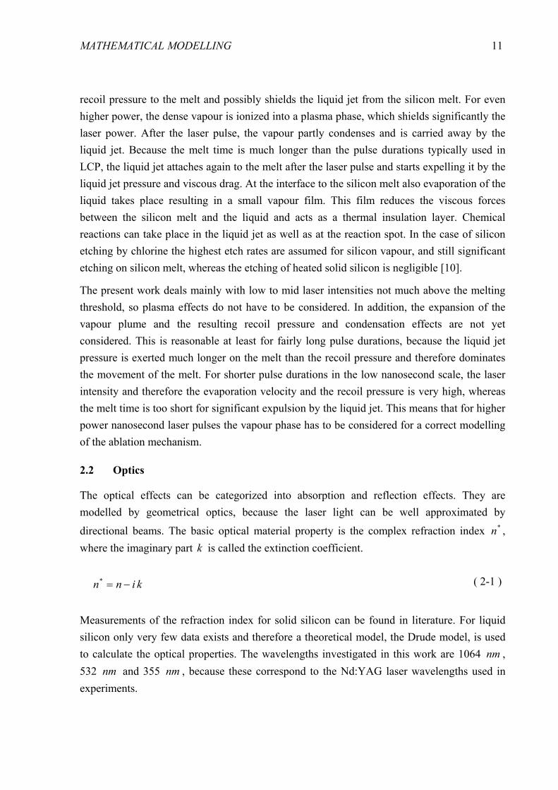
2.2 Optics
The optical effects can be categorized into absorption and reflection effects. They are modelled by geometrical optics, because the laser light can be well approximated by
directional beams. The basic optical material property is the complex refraction index *n , where the imaginary part k is called the extinction coefficient.
kinn −=* ( 2-1 )
Measurements of the refraction index for solid silicon can be found in literature. For liquid silicon only very few data exists and therefore a theoretical model, the Drude model, is used to calculate the optical properties. The wavelengths investigated in this work are 1064 nm , 532 nm and 355 nm , because these correspond to the Nd:YAG laser wavelengths used in experiments.

MATHEMATICAL MODELLING
12
2.2.1 Complex refraction index of silicon
For solid silicon, measured data for the optical properties has been taken from literature [32-34] and have been fitted to the expressions shown in Tab. 2-1.
λ [nm] n [33] k [32, 34]
1064 ][142.356.3 4 KTe−+ 414 ][27.1 KTe−
532 ][68.595.3 4 KTe−+ ⎟⎠⎞
⎜⎝⎛−
KTe
430exp1252.2 2
355 ][263.8856.5 4 KTe−− 2.9
Tab. 2-1: Solid silicon refraction index calculated from literature data
For liquid silicon no suitable measurements for the optical properties were found, therefore the Drude model is used as described in [35]. Liquid silicon can electronically be treated as a metal, because the same characteristic free electron gas exists. The optical properties are strongly dependent on the electrical ones, because incoming photons are mainly absorbed by the free carriers. Drude gave an expression for the frequency dependent complex permittivity of a free electron gas.
( ) ( )22
2
22
2* 1
γωωωγ
γωω
ε+
++
−= plpl if ( 2-2 )
The plasma frequency plω is a material specific constant value and the collision rate γ is a
temperature dependent value as proposed in [36].
λπω c2
=
mm T
Tγγ =
( 2-3 )
This results in a permittivity dependent on temperature and frequency. The required optical properties are related to the permittivity by the complex equation ( 2-4 ).
( ) *2* ε=n ( 2-4 )

MATHEMATICAL MODELLING
13
For the calculation of n and k by the Drude model data for liquid silicon is taken from [37]
to 11650.2 −= sepω and 1157170.4 −= semλ .
2.2.2 Absorption
Laser light absorption occurs due to excitation of atoms or molecules by the photon energy. For the laser wavelengths used, photons interact most dominantly with electrons. This means that one photon gives all its energy to one electron. For non-free electrons not all energy levels are allowed, therefore the absorption coefficient is strongly dependent on the electronic structure of the material and the wavelength. For example for the semiconductor silicon wavelengths near or above the band gap are weakly absorbed. Increasing temperature increase also the amount of free electrons, therefore the absorption coefficient is strongly increased, which can be seen in [32].
For high laser intensities, i.e. for high photon densities, the probability that more than one photon hits an electron is increased. This is called multiphoton absorption. The absorption coefficient is then dependent on the laser intensity. Further increase of the intensity leads to more free electrons, which absorb more laser light, leading to a further ionization. At a certain intensity level this ends up in avalanche ionization, called optical breakdown, where suddenly all of the light is absorbed. It is obvious that for LCP the optical breakdown has to be avoided in the liquid jet. Therefore only laser intensities can be used in LCP, which are below the optical breakdown threshold. For the wavelengths 1064 nm and 532 nm , this threshold in
water is at roughly 2100 cmGW [38]. For a µm50 jet diameter and a typical pulse energy of
mJ1 this would mean a critical pulse duration of roughly one nanosecond. Generally spoken
for LCP applications the laser pulse durations have to be at least in the nanosecond scale. Because of this restriction, multiphoton absorption in the silicon can also be neglected. It shows neglibible absorption coefficents for the allowed intensities, which can be derived from [39].
The basic quantity for modelling absorption effects is the absorption coefficient α , which can be calculated out of extinction coefficient and the wavelength of the light.
λπα k4
= ( 2-5 )
Laser light can be seen as unidirectional light. Even after crossing the surface and diffusing the light this approximation is feasible, because the absorption length is much smaller than the typical lateral width of the spatial intensity distribution. Therefore the absorption equation can be expressed in one dimension.

MATHEMATICAL MODELLING
14
IdzdI α−= ( 2-6 )
If the absorption coefficient is constant over the z -coordinate, equation ( 2-6 ) can be solved analytically. The solution shown in equation ( 2-7 ) is called the Lambert-Beer law.
( ) ( )zIzIz
α−==
exp0
( 2-7 )
In Fig. 2-4 the temperature dependent absorption coefficient of solid and liquid silicon at various wavelengths is shown.
0 1000 2000 3000 4000 500010
1
102
103
104
105
106
107
temperature [K]
abso
rptio
n co
effic
ient
[cm
−1 ]
355 nm532 nm1064 nm
Fig. 2-4: Absorption coefficient of silicon for different wavelengths as used in the simulations

MATHEMATICAL MODELLING
15
Fig. 2-5: Path enlargement by total reflection in the liquid jet
In the liquid jet another effect has to be considered. Because the laser light is coupled under an angle determined by the coupling optics, it partly travels not directly through the liquid jet as illustrated in Fig. 2-5. This results in an optical path enlargement depending on the angle between the actual light beam and the z - coordinate beamϕ . The relative path enlargement δ
is calculated by equation ( 2-8 ).
beamϕ
δcos
1= ( 2-8 )
The maximum angle allowed is determined by the critical angle to ensure total reflection. For water as surrounding medium the maximum relative path enlargement is 335.1max, =waterδ .
In the simulations the path enlargement is implemented by an effective absorption coefficient.
αδα =eff ( 2-9 )
2.2.3 Reflection
Reflection on the surface plays an important role in modelling of LCP, because it determines how much energy is coupled into the material. The amount of the non reflected laser light intensity is defined by the reflectivity R .
beamϕ
lens
nozzle opening
z

MATHEMATICAL MODELLING
16
( ) incsurf IRI −= 1 ( 2-10 )
A general beam reflection at an interface between material 1 and 2 is illustrated in Fig. 2-6. For a general angular reflection, the light beam has to be distinguished in a vertically and horizontally polarized part. The regarding reflectivity is then calculated by the Fresnel formulas ( 2-11 ) and ( 2-12 ) [40].
Fig. 2-6: Beam reflection at a flat interface between material 1 and material 2
( ) ( )( ) ( )
2
*2
*1
*2
*1
coscoscoscos
refrinc
refrinc
nnnn
Rϕϕϕϕ
+
−=⊥ ( 2-11 )
( ) ( )( ) ( )
2
*1
*2
*1
*2
|| coscoscoscos
refrinc
refrinc
nnnn
Rϕϕϕϕ
+
−= ( 2-12 )
The angle of refraction refrϕ is defined by the refraction indices and the incident angle incϕ .
⎟⎟⎠
⎞⎜⎜⎝
⎛= −
increfr nn
ϕϕ sinsin *2
*11 ( 2-13 )
For an arbitrary incident beam direction and an arbitrary surface normal direction the direction of the reflected beam can be calculated by the vector equation ( 2-14 ).
incϕ
refrϕ
*1n
*2n
incb
reflb
n

MATHEMATICAL MODELLING
17
( )nbnbb incincrefl ⋅−= 2 ( 2-14 )
In this case the incident angle is defined by the scalar product of surface normal and incident beam direction.
( )incinc bn ⋅−= −1cosϕ ( 2-15 )
In many cases the incident laser beam can be treated as perpendicular to the surface, i.e. when the ablated geometry shows no significant steepness. Furthermore, the surrounding medium is in our case transparent, which means that the extinction coefficient of the surrounding medium can be set to zero. The general Fresnel formulas then simplify to the well known reflectivity equation ( 2-16 ) independent of polarization.
( )( ) 2
22
21
22
221
knnknnR
+++−
= ( 2-16 )
The resulting perependicular reflectivity for silicon is plotted in Fig. 2-7 for air and water as surrounding medium.
0 1000 2000 3000 4000 50000.2
0.3
0.4
0.5
0.6
0.7
0.8
temperature [K]
refle
ctiv
ity
355 nm
532 nm
1064 nm
Fig. 2-7: Reflectivity of silicon for air (solid line) and water (dashed line) as surrounding medium

MATHEMATICAL MODELLING
18
A special treatment is needed for reflection at small films, like passivation layers on the front side of a silicon solar cell. Here multi-reflections between the material interfaces take place, which can be calculated for perpendicular incident light and a non-absorptive film material to an effective reflectivity [41].
( )( )
2
*2,
*,1
*2,
*,1
exp1exp
⎟⎟⎠
⎞⎜⎜⎝
⎛
+
+=
fff
ffff irr
irrR
δδ
( 2-17 )
1
1*,1 nn
nnr
f
ff −
−=
f
ff nn
nnr
−
−= *
2
*2*
2,
( 2-18 )
Here fδ is the optical path difference depending on wavelength, film refraction index and
film thickness fd .
λ
πδ ff
f
dn4= ( 2-19 )
Fig. 2-8: Sketch of multiple reflections at thin films.
1n
*2n
fn *,1 fr
*2,fr fd

MATHEMATICAL MODELLING
19
2.3 Thermodynamics
The modelling of thermodynamic effects in LCP incorporates heat transport, phase changes and species transport due to evaporation or diffusion.
2.3.1 Heat transport
As described before in section 2.2.2 the laser power is dominantly absorbed by the electrons. Before a uniform temperature for the electrons and the lattice is reached, the excited electrons have to transfer energy to the lattice. This relaxation happens on a picosecond timescale [35], which is much shorter than the used laser pulse durations of at least a few nanoseconds. So for simulation of LCP only one equal electron-lattice temperature field needs to be considered.
The general partial differential equation for transient heat transport ( 2-20 ) consists of a transient, a convection, a conduction and a source term. The convection term takes into account transport of heat due to material movement like the melt flow. The source term corresponds to the absorbed laser power, see equation ( 2-21 ).
( ) ( ) ( ) hpp STKTcvTcdtd
+∇∇=∇+ ρρ ( 2-20 )
ISh α= ( 2-21 )
For the description of heat transport in the liquid jet the spatial distribution of the temperature in the cross section area is approximated to be constant, so equation ( 2-20 ) can be reduced to the jet direction, i.e. the z -coordinate. This is feasible because of the high length to width ratio of the liquid jet on the order of a thousand, which leads to relatively high lateral heat conduction and temperature homogenization. Also the intensity profile is varying with jet length, which results in lateral homogenization by averaging. Furthermore, the velocity profile of the liquid jet is approximately flat [42] and so the velocity is only dependent on the z -coordinate. The heat capacity pc , the density ρ and the heat conductivity K are assumed
to be constant, so they can be placed in front of the derivatives resulting in equation ( 2-22 ).
hzpp Sdz
TdKdzdTvc
dtdTc +=+ 2
2
ρρ ( 2-22 )
The heat transport in silicon is described by the enthalpy-based heat transport equation ( 2-23 ), where the enthalpy is the inner energy density in units of energy per volume. This formulation is used as proposed, for example, by Grigoropoulus et al. [21]. During phase

MATHEMATICAL MODELLING
20
changes the temperature stays constant whereas the enthalpy is steadily changing, which is beneficial for implementation of a stable numerical time integration. Furthermore, for the implementation of the heat transport equation in silicon, no movement of silicon, i.e. melt flow, is considered, so the convection term can be removed.
( ) hSTKdt
dH+∇∇= ( 2-23 )
In equation ( 2-23 ) the temperature needs to be calculated from the enthalpy values. This dependency is defined by the integral ( 2-24 ) for arbitrary temperature dependent thermal properties.
( ) ∫=T
p dTcTH0ρ ( 2-24 )
Due to phase changes, this integral is defined only stepwise. For solid silicon the temperature dependent heat capacity and density is taken from [43]. The data has been extrapolated to show a zero enthalpy value at the absolute zero point. This dependency is not physically correct, but does not affect the calculation of the temperature field above room temperature. Additionally, this formulation shows a better numerical convergence than setting the enthalpy to zero at room temperature. A fit was performed to achieve a second order polynomial for the
temperature enthalpy relation of solid silicon with 26171 375.2 JmKec −−= ,
JmKec 372 512.5 −= and Kc 06.983 = . A plot of the relation ( 2-25 ) is shown in Fig. 2-10.
322
1 cHcHcTs ++= ( 2-25 )
Another heat transport effect is the surface cooling, which can occur by radiation and combined conductive and convective cooling. At the hot silicon surface, the radiation heat loss is determined by the Stefan-Boltzmann law neglecting the incoming radiation ( 2-26 ).
( )44envsurfTsurf TTJ −= σε ( 2-26 )
For conductive cooling or combined conductive and convective cooling, the surface heat transfer is approximately linearly dependent on the temperature difference of the two neighbouring materials. This can described by the heat transfer coefficient ht .
MATHEMATICAL MODELLING
21
( )envsurfsurf TThtJ −= ( 2-27 )
The heat transfer coefficient is dependent on the thermal material properties, and for convection cooling, also on the velocity field of the cooling fluid. This means that for a specific setup the unknown heat transfer coefficient has to be derived either from measurements or calculations. In the case of cooling by a liquid impinging jet, some data can be found in literature [44], but can not be applied to the LCP case because of different jet types and different parameter values, especially Reynolds numbers.
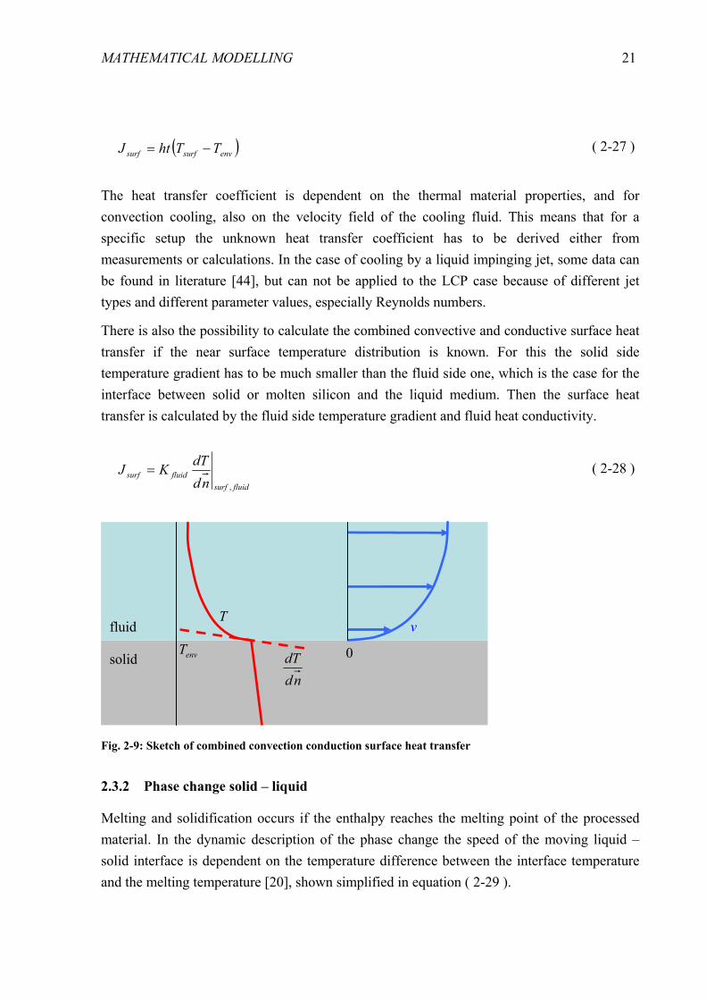
There is also the possibility to calculate the combined convective and conductive surface heat transfer if the near surface temperature distribution is known. For this the solid side temperature gradient has to be much smaller than the fluid side one, which is the case for the interface between solid or molten silicon and the liquid medium. Then the surface heat transfer is calculated by the fluid side temperature gradient and fluid heat conductivity.
fluidsurf
fluidsurfnd
dTKJ,
= ( 2-28 )
Fig. 2-9: Sketch of combined convection conduction surface heat transfer
2.3.2 Phase change solid – liquid
Melting and solidification occurs if the enthalpy reaches the melting point of the processed material. In the dynamic description of the phase change the speed of the moving liquid – solid interface is dependent on the temperature difference between the interface temperature and the melting temperature [20], shown simplified in equation ( 2-29 ).
v T
nddT
0 envT fluid
solid

MATHEMATICAL MODELLING
22
( ) ⎟⎟⎠
⎞⎜⎜⎝
⎛⎟⎟⎠
⎞⎜⎜⎝
⎛ −−−Κ=
sl
msl
mB
mslsl T
TTTk
LTv exp1 ( 2-29 )
This means, that the phase change takes place not exactly at the melting temperature, but some superheating or undercooling is needed. The kinetic rate constant Κ for melting is generally much higher than for solidification, because of the high activation energy for crystallization. In the simulations of the present work solidification velocities show values not higher than sm5 . Using the data reported in [45] results in a maximum undercooling of
K75 . This work aims to approximately describe the physical effects rather than giving highly
exact solutions, so this amount of undercooling is feasible to neglect. The superheating for melting is even lower, so for the present work the phase change solid – liquid is assumed to take place exactly at phase change temperature. In addition, the solidification speeds are lower than the critical value for amorphization of silicon of sm15 reported in [45]. This ensures
that the silicon solidifies to a crystal rather than to an amorphous state for any LCP parameters.
Assuming a defined melting point, the phase change can be described by an enthalpy based approach. Once the melting temperature mT is reached, the temperature stays constant while
the enthalpy further in- or decreases until the latent heat of melting mL has been overcome.
For silicon the latent heat of melting is taken from [46] to molkJL mmol 50, = . Because the
variable to be solved for heat transport is the enthalpy in units of energy per volume, the latent heat has to be adopted according to equation ( 2-30 ).
M
LL molρ
= ( 2-30 )
In the liquid state the product of heat capacity and density of silicon shows a constant value of 36432.2 mJec p =ρ [21]. This results in the linear relation ( 2-31 ) between enthalpy and
temperature with pcc ρ14 = and pmmm cLHTc ρ)(5 +−= , shown in Fig. 2-10. mH is the
enthalpy where melting starts, and is calculated by inserting mT in equation ( 2-25 ).
54 cHcT += ( 2-31 )

MATHEMATICAL MODELLING
23
2.3.3 Evaporation
For the second phase change liquid – vapour of silicon two different models are used, mainly dependent on the speed of evaporation. For low evaporation speed, i.e. for relatively low laser intensities, the material evaporates by so called normal boiling [47]. Here the evaporation takes place exactly at the boiling temperature, so an enthalpy based description as discussed above can be used. This means that the material is assumed to be fully evaporated if the boiling point at vH is reached and additionally the latent heat of vaporization vL has been
overcome. According to [47], this model is valid for laser pulse duration of greater than roughly one microsecond.
For higher laser light intensities, significant superheating occurs and can no longer be neglected. Therefore a dynamical description of the phase change is required, which means a calculation of the evaporation speed. For nanosecond laser pulses usually the Hertz-Knudsen equation ( 2-32 ) is used. Here the evaporation rate of atoms is set to the effusion rate derived from statistical thermodynamics [48].
lvBa
sat
Tkmp
nπ2
=& ( 2-32 )
To calculate the surface recession velocity lvv , equation ( 2-32 ) has to be divided by the atom
density of the liquid al mρ . In addition it is assumed that the material does not evaporate
into vacuum, but directly above the liquid surface a small layer of pure vapour exists, which is feasible within the laser pulse duration. The evaporation speed is then approximately calculated by the difference of saturation pressure and partial pressure at the surface. In this work no vapour dynamics are modelled and the partial pressure is set to an externally calculated value extp . This way an environmental pressure or a pressure distribution caused
by the impinging jet can be taken into account.
a
lvBl
extsatlv
mTk
ppv
πρ
2−
= ( 2-33 )
Equation ( 2-33 ) results generally in an increasing evaporation speed with temperature, because the saturation pressure is strongly dependent on temperature. For the case of silicon no measured data for the saturation pressure above the boiling point exists, so the Clausius-Clapeyron equation ( 2-34 ) is used assuming a constant molar latent heat of vaporization

MATHEMATICAL MODELLING
24
vmolL , . For silicon vmolL , is calculated by the data given in [49] to molkJ400 at the boiling
point.
⎟⎟⎠
⎞⎜⎜⎝
⎛⎟⎟⎠
⎞⎜⎜⎝
⎛−−=
b
vmolsat TTR
Lpp 11exp ,
0 ( 2-34 )
For reasons of energy conservation, the latent heat of vaporization has to be considered additionally as a surface heat flux during evaporation.
vLq vlv = ( 2-35 )
In Fig. 2-10 the entire relation of temperature and enthalpy for silicon as used in the present work is shown. Beyond the boiling point the horizontal curve corresponds to the normal boiling model, whereas for the Knudsen evaporation the further increasing curve illustrates the effect of superheating.
Fig. 2-10: Temperature – enthalpy relation as used in the simulations; the dashed curve corresponds to the superheating for the Knudsen evaporation model and the solid one to the enthalpy based model
The Knudsen evaporation as described above is still a quite simplified model, because the influence of the surrounding vapour is not considered. Especially for higher laser intensities the generated vapour plume results in high recoil pressures and directly influences the evaporation speed. A good model would be the so called Knudsen layer as proposed by Knight [50]. Here it is considered that the temperature and the pressure in a small layer above
solid
liqui
d
0 10 20 30 40 500
500
1000
1500
2000
2500
3000
3500
4000
4500
5000
enthalpy [J/mm³]
tem
pera
ture
[K]

MATHEMATICAL MODELLING
25
the surface are not in thermodynamic equilibrium, which can be treated as a jump condition. But using this model would require a coupled solving of gas dynamics, which is not done within the present work. Also condensation can not be calculated without gas dynamics, because the actual partial pressure at the surface has to be known.
2.3.4 Species transport
Two different effects of species transport are modelled. One is the transport of chemical additives in the liquid jet. Here mainly the light induced generation and transport of chlorine radicals is of interest. At the reaction spot the diffusion of impurity atoms in the liquid silicon is modelled, because this is the basic mechanism for the doping process.
The general transient species transport equation ( 2-36 ) includes similar to the heat transport equation a convection, a conduction and a source term. The variable to be solved is the concentration of species particles C .
spSCDCvdtdC
+Δ=∇+ ( 2-36 )
In solid silicon the diffusion coefficient is strongly temperature dependent. Usually time scales of hours are needed to diffuse a typical phosphorous emitter for silicon solar cells. For liquid silicon an increase of the diffusion coefficient of several orders of magnitude takes place, which is shown for phosphorous in Fig. 2-11 with data taken from [51] for solid silicon and [19] for liquid silicon respectively. This jump is the reason why even within the very short melt times below one microsecond produced by laser pulses, a usable amount of impurity atoms diffuses into the silicon. On the other hand, this jump clearly allows for the solid state diffusion to be neglected in the modelling of laser doping. The liquid silicon diffusion coefficient is assumed to be constant. Because liquid phase diffusion is dominated by the size of the impurity atom [48], which is temperature independent, this approximation is feasible. The melt is during its lifetime dominantly at melting temperature as shown later in this work. This further reduces the error of the final species distribution introduced by the simplified temperature independent diffusion coefficient.

MATHEMATICAL MODELLING
26
1000 1500 2000 2500 300010
−14
10−12
10−10
10−8
10−6
10−4
10−2
temperature [°C]
diffu
sion
coe
ffici
ent [
cm²/
s]
Fig. 2-11: Temperature dependent diffusion coefficient of phosphorous in solid and liquid silicon
If flow is not considered, the convection term in equation ( 2-36 ) can be removed. Also in the material volume no sources for impurity atoms are present. These simplifications result in the well known Fick’s law ( 2-37 ), which is used to calculate impurity atom diffusion in silicon melt.
CDdtdC
Δ= ( 2-37 )
Different boundary conditions for species transport are used in this work. They can be divided into isolating, infinite source and finite source. For the isolating case no species flux over the boundary is allowed, which is for example the case at the liquid – solid interface in silicon.
0=surfnd
dC ( 2-38 )
The infinite source boundary condition is used at the liquid jet outlet and at the silicon surface if an unlimited dopant source is assumed.
bcsurfCC = ( 2-39 )

MATHEMATICAL MODELLING
27
In dry laser doping a phosphorous containing precursor layer is used as the dopant source, see section 5.5. This has to be modelled by a finite source boundary condition. Here a surface concentration dependent on the loading Θ , which transiently decreases by the dopant flux through the surface, is used. Because no suitable physical model was found, a linear relationship starting from saturation concentration in silicon melt at full loading and decreasing to zero at zero loading is assumed, see equation ( 2-40 ). Comparing the simulation with experimental results shows that this approximation describes the doping by a precursor layer source in a reasonable way.
0=Θ
Θ=
tsatsurf
CC ( 2-40 )
For doping with LCP an infinite source boundary condition is used. The surface concentration is a free parameter and is adjusted in the simulation to fit the experimental results. Much better would be a boundary condition which can be calculated by the dopant concentration in the liquid jet. The first idea, that this surface concentration is equal or proportional to the dopant concentration in the liquid jet, gives no suitable results. Here the surface concentration of the measured doping profiles should be proportional to the dopant concentration of the solvent, which is not the case for the different measured doping profiles. Therefore, the processes at the solvent – silicon interface has to be modelled in more detail. This means considering the thermal atomization of the dopant and the dopant transport by diffusion and convection in the near interface region. This could not be done within the timeframe of the present work, so the surface concentration remains as a free parameter for LCP doping simulations.
The optical properties of silicon are generally influenced by the doping level. This is not considered in the present work, because no data has been found in literature which covers the needed concentration and temperature range. This is assumed to introduce a negligible error, because the laser light interacts mainly with the lowly doped silicon bulk, and in the liquid phase the absorption is nevertheless very high.
2.4 Fluid dynamics
For simulation of fluid flow the commercial software Fluent is used. The models and regarding equations shown in this section are taken from the Fluent manual [52], where references to literature are included.
MATHEMATICAL MODELLING
28
2.4.1 Basic fluid flow
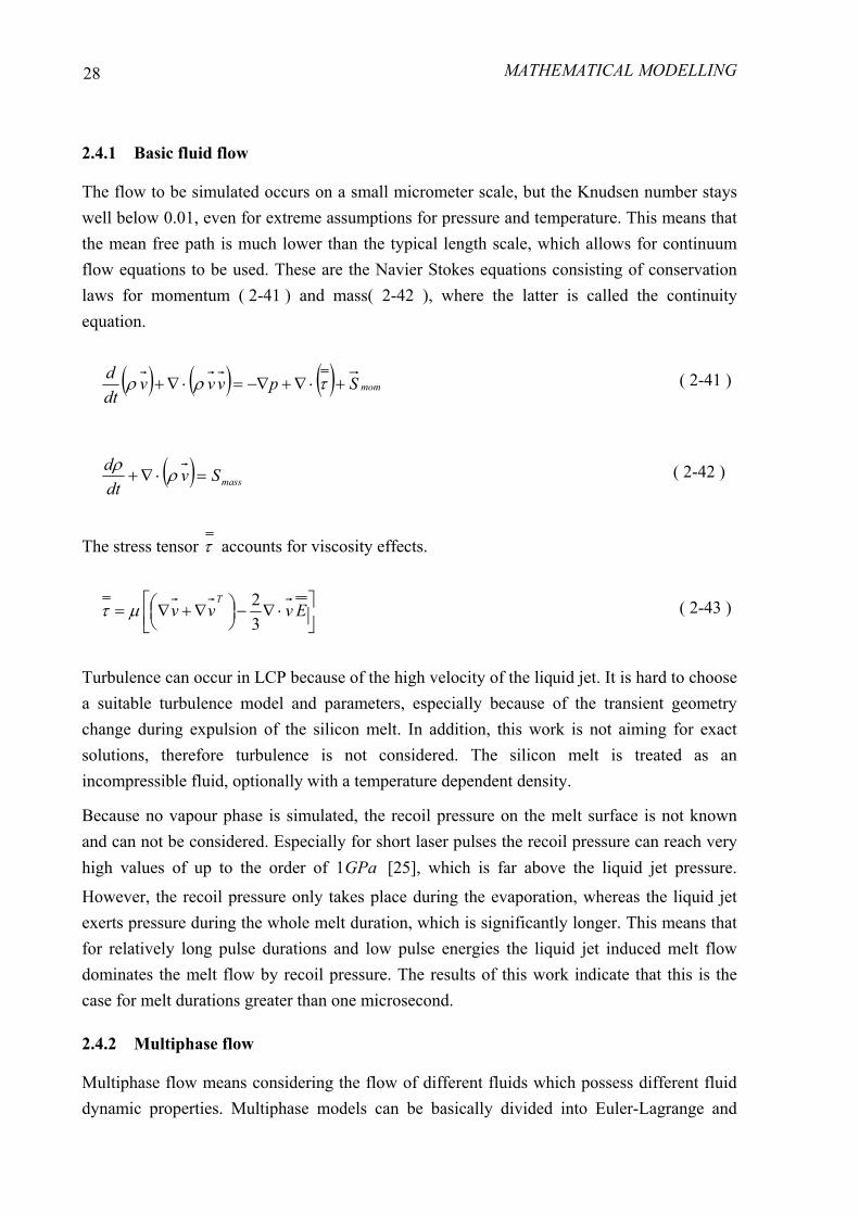
The flow to be simulated occurs on a small micrometer scale, but the Knudsen number stays well below 0.01, even for extreme assumptions for pressure and temperature. This means that the mean free path is much lower than the typical length scale, which allows for continuum flow equations to be used. These are the Navier Stokes equations consisting of conservation laws for momentum ( 2-41 ) and mass( 2-42 ), where the latter is called the continuity equation.
( ) ( ) ( ) momSpvvvdtd
+⋅∇+−∇=⋅∇+ τρρ ( 2-41 )
( ) massSvdtd
=⋅∇+ ρρ ( 2-42 )
The stress tensor τ accounts for viscosity effects.
⎥⎦⎤
⎢⎣⎡ ⋅∇−⎟
⎠⎞⎜
⎝⎛ ∇+∇= Evvv
T
32μτ ( 2-43 )
Turbulence can occur in LCP because of the high velocity of the liquid jet. It is hard to choose a suitable turbulence model and parameters, especially because of the transient geometry change during expulsion of the silicon melt. In addition, this work is not aiming for exact solutions, therefore turbulence is not considered. The silicon melt is treated as an incompressible fluid, optionally with a temperature dependent density.
Because no vapour phase is simulated, the recoil pressure on the melt surface is not known and can not be considered. Especially for short laser pulses the recoil pressure can reach very high values of up to the order of GPa1 [25], which is far above the liquid jet pressure.
However, the recoil pressure only takes place during the evaporation, whereas the liquid jet exerts pressure during the whole melt duration, which is significantly longer. This means that for relatively long pulse durations and low pulse energies the liquid jet induced melt flow dominates the melt flow by recoil pressure. The results of this work indicate that this is the case for melt durations greater than one microsecond.
2.4.2 Multiphase flow
Multiphase flow means considering the flow of different fluids which possess different fluid dynamic properties. Multiphase models can be basically divided into Euler-Lagrange and
MATHEMATICAL MODELLING
29
Euler-Euler models. In the Euler-Lagrange approach, algebraic equations of motion are solved for discrete particles interacting with a continuous flow field. In the Euler-Euler model, two or more interpenetrating continuous flow fields are considered. In LCP mainly the flow of the liquid jet interacting with the silicon melt is of interest, which corresponds to the Euler-Euler model. Silicon melt and liquid solvents are treated as immiscible fluids, therefore a sharp interface exists and surface tension has to be taken into account.
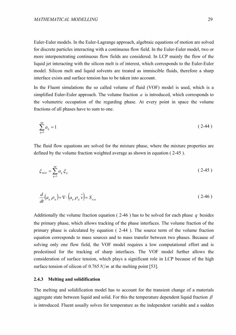
In the Fluent simulations the so called volume of fluid (VOF) model is used, which is a simplified Euler-Euler approach. The volume fraction a is introduced, which corresponds to the volumetric occupation of the regarding phase. At every point in space the volume fractions of all phases have to sum to one.
∑=
=np
qqa
11 ( 2-44 )
The fluid flow equations are solved for the mixture phase, where the mixture properties are defined by the volume fraction weighted average as shown in equation ( 2-45 ).
∑=
=np
qqqmixt a
1ξξ ( 2-45 )
( ) ( ) qaqqqq Svaadtd
,=⋅∇+ ρρ ( 2-46 )
Additionally the volume fraction equation ( 2-46 ) has to be solved for each phase q besides
the primary phase, which allows tracking of the phase interfaces. The volume fraction of the primary phase is calculated by equation ( 2-44 ). The source term of the volume fraction equation corresponds to mass sources and to mass transfer between two phases. Because of solving only one flow field, the VOF model requires a low computational effort and is predestined for the tracking of sharp interfaces. The VOF model further allows the consideration of surface tension, which plays a significant role in LCP because of the high surface tension of silicon of mN765.0 at the melting point [53].
2.4.3 Melting and solidification
The melting and solidification model has to account for the transient change of a materials aggregate state between liquid and solid. For this the temperature dependent liquid fraction β
is introduced. Fluent usually solves for temperature as the independent variable and a sudden

MATHEMATICAL MODELLING
30
solidification at the exact melting temperature would cause numerical problems. Therefore a mushy region mTΔ is defined around the melting point, where the material is linearly
changing from solid to liquid.
⎟⎟⎟⎟
⎠
⎞
⎜⎜⎜⎜
⎝
⎛
⎟⎟⎟⎟
⎠
⎞
⎜⎜⎜⎜
⎝
⎛
Δ
Δ−−
= 0,1,2minmaxm
mm
T
TTT
β ( 2-47 )
To hinder movement in the solid state, a very high momentum sink is added to equation ( 2-48 ). The sink is dependent on the liquid fraction in such a way that for a liquid fraction of one, the value of the sink is zero. The nonlinear expression is optimized for numerical stability.
( ) veS mom
53
2
1001.0
1+−
=β
β ( 2-48 )
2.5 Chemistry
Chemical effects modelled in the present work comprise photochemical decomposition of molecules and reaction kinetics. The focus is on effects in the liquid jet, mainly the generation and recombination of chlorine radicals. At the reaction spot extreme conditions in terms of time scale and temperature occur. Here no suitable data for surface reaction kinetics exists, which makes a quantitative simulation impossible.
2.5.1 Photochemical radical generation
If photon energies are high enough, the laser light is able to crack molecule bonds. This can be used to produce chlorine radicals out of molecular chlorine in the liquid jet. The amount of radicals generated equals the product of quantum efficiency dΦ and the amount of photons
absorbed by the molecular chlorine, which is the absorbed laser power divided by the photon energy [54].
chI
S CldCl
λα2Φ=⋅ ( 2-49 )
The absorption coefficient of molecular chlorine is calculated by the collision cross section
cσ .

MATHEMATICAL MODELLING
31
cClCl C σα22
= ( 2-50 )
Data for chlorine radical generation with nm355=λ has been taken from [54] to 35.0=Φ d
and 21994.1 cmec−=σ .
2.5.2 Reactions
Many reactions can take place during LCP, for example etching and oxidation of hot silicon, thermal decomposition of dopant sources and reactions of chemical active additives in the liquid jet. At the reaction spot mainly interfacial reactions occur, which are more complex to model than volumetric reactions. Additionally, for the extreme scales of temperature and time no suitable literature data for reaction kinetics can be found. Therefore no attempt was made within the present work for quantitative modelling of the reaction kinetics at the reaction spot.
In contrast to the reaction spot the conditions in the liquid jet are much easier. Here the generation of chlorine radicals is modelled as mentioned in the previous section. Once created, the radicals show a high recombination rate, which can be described by a basic
reaction with the kinetic rate constant )(1.1 10, smollek ClClr =⋅−⋅ [54]. Furthermore, the
radicals can react with the solvent used as the liquid media. For the solution of gases organic solvents are usually the first choice. In [55] kinetic rate constants for the reaction of chlorine radicals with different organic solvents are shown to be in the region of
)(10..10 97, smollk solvClr =−⋅ . This is somewhat below the radical recombination rate, but still
has to be considered. In [10] it has been shown that the best suitable solvents are the perflourinated carbon compounds, not least because of their chemical stability. In this case the reaction of the solvent and the chlorine radicals can be readily neglected. The recombination is treated as a sink of radical concentration, which is calculated by equation ( 2-51 ).
2,2 ⋅⋅−⋅⋅ −= ClClClrACl CkNS ( 2-51 )
The reactions regarded in this work are exothermal and have to be considered as heat sources. The heat source is calculated by the reaction enthalpy HΔ of reactants 1 and 2, as shown in equation ( 2-52 ). In case of chlorine radical recombination the reaction enthalpy corresponds to the enthalpy of formation of molecular chlorine molkJH Clr 243
2, =Δ [48].
rrAh HCCkNS Δ= − 2121,2 ( 2-52 )

32
3 Fundamentals of the simulation methods
In this work essentially two different ways of solving the mathematical models are used. One way is the programming of a finite differences solver. The advantage over commercial software is the ability to change and extend the program code, which enables the possibility of basic solver customization and adaption to the regarding models. Arbitrary equations of different kinds, like for example the equation of laser light absorption and the heat transport equation, can be implemented and simultaneously solved. This results in an overall high problem adaption and speed of the simulation code. The theory of finite differences described in this section is taken from [56].
The second way to simulate LCP is by using the commercial software Fluent by Ansys, Inc. Fluent is a powerful tool basically for solving fluid flow equations, but has also implemented models for other physics like heat transport, species transport etc. Implementing an efficient solver code for the complex fluid flow equations by basic programming requires high effort, so using the highly developed Fluent solver is a reasonable way for the simulation of fluid flow in LCP. Fluent also offers the possibility of customization by adding user defined C code, which is used for example for the transient coupling of Fluent with Matlab.
3.1 PDE solving by finite differences
The basic transient equations to be solved in this work by finite differences show the form of the general transport partial differential equation (PDE) for a scalar Ψ with diffusion term and source term S .
( ) Sdtd
+Ψ∇Γ∇=Ψ
( 3-1 )
Rewriting the equation in Cartesian coordinates yields equation ( 3-2 ).
Sdzd
dzd
dyd
dyd
dxd
dxd
dtd
+⎟⎠⎞
⎜⎝⎛ ΨΓ+⎟⎟
⎠
⎞⎜⎜⎝
⎛ ΨΓ+⎟
⎠⎞
⎜⎝⎛ ΨΓ=
Ψ ( 3-2 )
The diffusion term can be approximated by finite differences for a known spatial distribution of Ψ at time t . The sources have also to be computable by Ψ and t . Equation ( 3-1 ) can
FUNDAMENTALS OF THE SIMULATION METHODS
33
then be solved by choosing proper starting values for Ψ and t followed by numerical time integration.
3.1.1 Spatial discretization
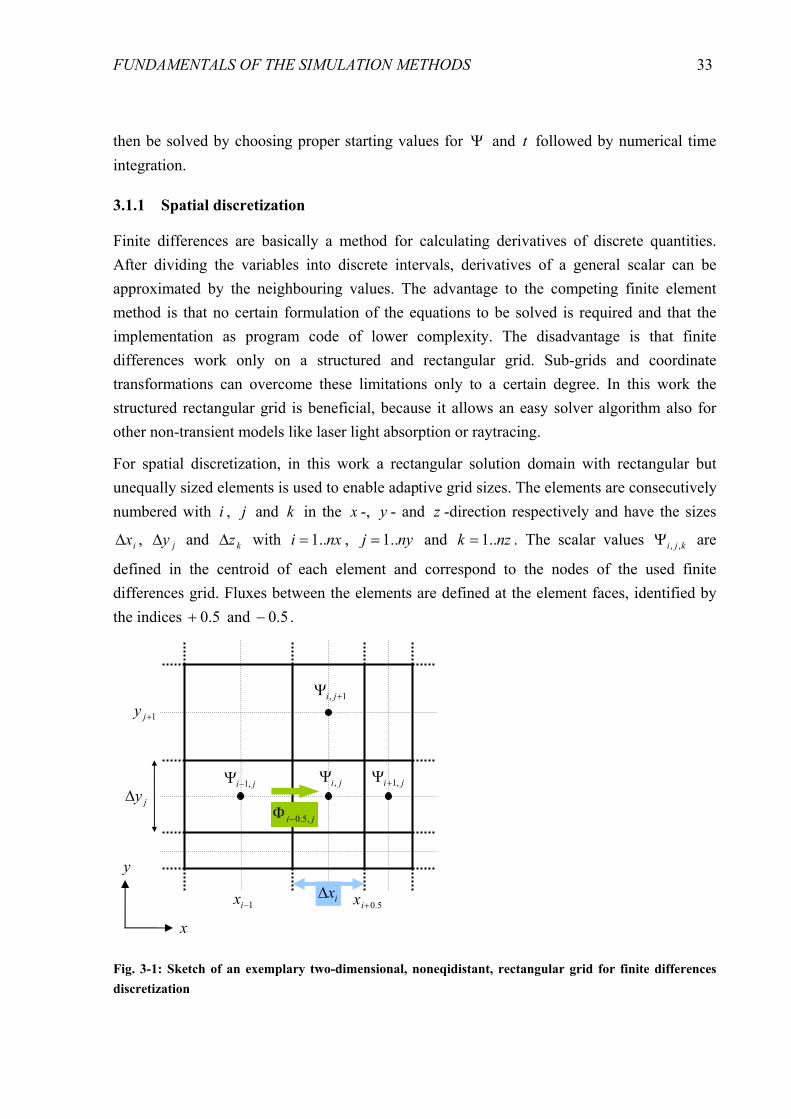
Finite differences are basically a method for calculating derivatives of discrete quantities. After dividing the variables into discrete intervals, derivatives of a general scalar can be approximated by the neighbouring values. The advantage to the competing finite element method is that no certain formulation of the equations to be solved is required and that the implementation as program code of lower complexity. The disadvantage is that finite differences work only on a structured and rectangular grid. Sub-grids and coordinate transformations can overcome these limitations only to a certain degree. In this work the structured rectangular grid is beneficial, because it allows an easy solver algorithm also for other non-transient models like laser light absorption or raytracing.
For spatial discretization, in this work a rectangular solution domain with rectangular but unequally sized elements is used to enable adaptive grid sizes. The elements are consecutively numbered with i , j and k in the x -, y - and z -direction respectively and have the sizes
ixΔ , jyΔ and kzΔ with nxi ..1= , nyj ..1= and nzk ..1= . The scalar values kji ,,Ψ are
defined in the centroid of each element and correspond to the nodes of the used finite differences grid. Fluxes between the elements are defined at the element faces, identified by the indices 5.0+ and 5.0− .
Fig. 3-1: Sketch of an exemplary two-dimensional, noneqidistant, rectangular grid for finite differences discretization
y
x
ji,Ψ ji ,1+Ψ ji ,1−Ψ
1, +Ψ ji
ixΔ
jyΔ
1−ix
1+jy
5.0+ix
ji ,5.0−Φ

FUNDAMENTALS OF THE SIMULATION METHODS
34
Defined by which neighbouring values are used, different discretization schemes, namely forward, backward and central differences exist. A higher order of difference expressions can be applied, which improves the accuracy and is achieved by taking a higher number of neighbouring scalar values into account. For a second order expression for example, the neighbouring values of a neighbour are additionally taken into account. In this work mostly first order formulations were chosen, because it is best suitable if some unsteadiness of a scalar occurs, like e.g. for the temperature at the liquid – solid interface.
Formulations of finite difference derivatives are shown in examples for the positive x -direction only. If the first derivative of an element is needed, the central difference scheme ( 3-3 ) is used. The gradient in x -direction at jy , 5.0+ix , which is the element face between
element ji, and ji ,1+ , is calculated by the forward scheme ( 3-4 ).
11
,,1,,1
,, −+
−+
−
Ψ−Ψ=
Ψ
ii
kjikji
kji xxdxd
( 3-3 )
ii
kjikji
kji xxdxd
−
Ψ−Ψ=
Ψ
+
+
+ 1
,,,,1
,,5.0
( 3-4 )
Multiplication of the gradient and the diffusivity results in the flux Φ through the corresponding element face.
kji
kjikji dxd
,,5.0,,5.0,,5.0
+++
ΨΓ=Φ ( 3-5 )
kjikji
kjikjikji
,,,,1
,,,,1,,5.0
2Γ+Γ
ΓΓ=Γ
+
++ ( 3-6 )
As proposed in [16], the diffusivity at the element faces are calculated according to equation ( 3-6 ) by so called harmonic averaging rather than arithmetic averaging, because this formulation best ensures conservation of the scalar. The diffusion term is then calculated by the flux differences according to equation ( 3-7 ). This further ensures the conservation of Ψ , which was identified to be more essential in laser heating than having a possibly higher accuracy approximation by applying a different discretization scheme of the diffusion term.

FUNDAMENTALS OF THE SIMULATION METHODS
35
i
kjikji
kji xdxd
dxd
Δ
Φ−Φ=⎟
⎠⎞
⎜⎝⎛ ΨΓ −+ ,,5.0,,5.0
,,
( 3-7 )
In this work problems with axial symmetry have to be solved, therefore cylindrical coordinates neglecting the azimuth coordinate are used. For simplicity and following the program code, no new coordinate names are introduced. y is handled as the azimuth
coordinate, which is neglected, and z as the height coordinate. x has the same direction of the radial coordinate r with an offset 0x , which corresponds to the centre of the axial symmetry,
i.e. where the radius equals zero, 0xxr −= . This allows changing the centre of axial
symmetry while keeping the same grid. The formulas for the spatial derivatives in the z -coordinate are not affected by going to cylindrical coordinates, whereas the diffusion term for the x -coordinate has to be adopted according to equation ( 3-8 ).
( )k
kiki
ii
kiikiikji zxr
rrΔ
Φ−Φ+
Δ
Φ−Φ=Ψ∇Γ∇ −+−−++ 5.0,5.0,,5.05.0,5.05.0
,, ( 3-8 )
Boundary conditions are applied by setting suitable values outside the boundary. For 1=i and nxi = , the values at 1−i and 1+i do physically not exist and are set to boundary values
bcΨ defined by the boundary conditions. For example an isolating boundary condition, which
corresponds to a zero value of the Neumann boundary condition, is applied by setting the outside values equal to the inside values. This boundary condition is also applied on a symmetrical plane within a 3d domain.
0
,5.0
=Ψ
= jidxd
⇒ jibcj ,1,0 =Ψ=Ψ=Ψ
( 3-9 )
Also Dirichlet boundary conditions are used, which means a constant scalar value on the boundary surface.
surfjnxi
Ψ=Ψ+= ,5.0
⇒ surfbcjnx Ψ=Ψ=Ψ + ,1 ( 3-10 )

FUNDAMENTALS OF THE SIMULATION METHODS
36
3.1.2 Time integration
Once the right hand side of equation ( 3-1 ) is expressed by Ψ and t , the time derivative in each element of the solution domain can be calculated. The time is divided into discrete time steps. After choosing proper starting values, the new values for Ψ and t after the first time step can be evaluated by different methods out of the time derivative. The new values are then used for calculation of the next time step and so on. This way a defined time span can be solved iteratively, which is called numerical integration.
The simplest numerical integration method is the Euler explicit or forward Euler method. Here the time derivative is calculated from the scalar values at time n and is multiplied by the time step size. The scalar values at the updated time 1+n are then simply calculated by adding.
tdt
d nnn Δ
Ψ+Ψ=Ψ +1 ( 3-11 )
The term „explicit“ means that the updated scalar values can be explicitly calculated from the previous ones, and no iterations are needed. Because of this, explicit time integration is very fast in calculating one time step. However, a strict limitation exists for the upper size of the time step size to ensure convergence of the finite difference algorithm. This maximum time step size can be derived from the Cauchy criterion ( 3-12 ).
( )
ΓΔΔΔ
≤Δ6
,,min 2
expzyxt l ( 3-12 )
Here the minimum size of all grid elements decides the limit of the time step size. The dependency on the grid size is quadratic, so by using finer grids, much more time steps are needed for the integration over a specific time span, which increases the overall computing time.
An improved explicit time integration method is the Runge-Kutta method. Here the time derivatives for several different time steps are averaged in a special way. In this work the fourth order Runge-Kutta method is used, which is defined in equations ( 3-13 ). In comparison to the first order Euler explicit method the accuracy of the solution is improved significantly, but is in the same way restricted to the maximum explicit time step size.
FUNDAMENTALS OF THE SIMULATION METHODS
37
21, t
dtd n
nn ΔΨ+Ψ=Ψ
2
1,2, t
dtd n
nn ΔΨ+Ψ=Ψ
tdt
d nnn Δ
Ψ+Ψ=Ψ
2,3,
tdt
ddt
ddt
ddt
d nnnnnn Δ⎟⎟
⎠
⎞⎜⎜⎝
⎛ Ψ+
Ψ+
Ψ+
Ψ+Ψ=Ψ +
3,2,1,1 22
61
( 3-13 )
Aside from explicit time integration, implicit schemes can be used. Implicit means that the updated scalar values can not be explicitly calculated, because the time derivative is dependent on the unknown updated instead of the previous scalar values. The resulting implicit equations have to be solved by numerical iteration. The advantage of implicit integration is that no mathematical restriction as to the time step size exists. Especially for small grids much greater time step sizes compared to the explicit ones can be applied, which can result in an overall lower computation time.
The most simple implicit time integration method is the Euler implicit or backward Euler method. Equation ( 3-14 ) has to be solved iteratively in each time step.
tdt
d nnn Δ
Ψ+Ψ=Ψ
++
11 ( 3-14 )
The first order methods, both explicit and implicit, show a numerical error because they use for evaluation of the time derivative either the scalar values at the beginning or the end of a time step. A more accurate approximation is to use the scalar values in the middle of the time step, which can be calculated by averaging the implicit and explicit time derivative, see equation ( 3-15 ). This is called the Crank-Nicolson method. It shows no time step size limitation and the effort for iterative solving is the same as for the Euler implicit method.
tdt
ddt
d nnnn Δ⎟⎟
⎠
⎞⎜⎜⎝
⎛ Ψ+
Ψ+Ψ=Ψ
++
11
21
( 3-15 )
FUNDAMENTALS OF THE SIMULATION METHODS
38
3.1.3 Alternating direction explicit (ADE) method
For finite differences a special time integration method, the alternating direction explicit method (ADE), exists, which combines the advantages of the explicit and implicit integration [56]. With this method an explicit calculation without time step restriction is possible. Therefore the ADE method has a big potential to speed up the time integration, especially for fine grids where the explicit time step would be very small.
The basic ADE formulas for solving equation ( 3-1 ) are shown below for two dimensions, a constant diffusivity Γ and an equidistant grid. They are derived from the so-called multilevel discretization of equation ( 3-1 ). Two different scalars U and V are introduced, which equal
Ψ at time n, nji
nji
nji VU ,,, Ψ== .
5.0,2
11,
1,,1,
2
1,1
1,,,1,
1, +
+−
++
+−
++
+
+Δ
+−−Γ+
Δ
+−−Γ=
Δ
− nji
nji
nji
nji
nji
nji
nji
nji
nji
nji
nji S
yUUUU
xUUUU
tUU
5.0,2
1,,1
,11,
2,1,
1,
1,1,
1, +−
+++−
+++
+
+Δ
+−−Γ+
Δ
+−−Γ=
Δ
− nji
nji
nji
nji
nji
nji
nji
nji
nji
nji
nji S
yVVVV
xVVVV
tVV
( 3-16 )
Equations ( 3-16 ) can be solved for 1,+njiU and 1
,+njiV . Starting from 1=i and 1=j by
consecutive increment of i and j , the calculation of 1,+njiU in each element uses the
previously updated values 1,1
+−n
jiU and 11,
+−
njiU . The same is done for V by starting at nxi = and
nyj = , following the opposite direction. Fig. 3-2 illustrates the meaning of the directions
used by the ADE algorithm.

FUNDAMENTALS OF THE SIMULATION METHODS
39
Fig. 3-2: Illustration of opposite calculation directions by ADE method
Using both previous and updated values for the calculation of the updated ones shows the mixed explicit and implicit character of the ADE method and explains the abolition of the time step restriction. Finally the updated scalar value is calculated by averaging U and V .
2
1,
1,1
,
+++
+=Ψ
nji
njin
ji
VU ( 3-17 )
3.2 Fluent
The reason for using the commercial software Fluent is because it is one of most highly developed solvers for fluid flow available. This ensures on the one hand an accurate and efficient simulation of fluid flow. On the other hand, the user interface enables a much faster and flexible method of grid generation and problem setup than could be accomplished by basic programming. Various additional models are available and selectable through the user interface. Especially the ability of simulating multiphase flow with free surfaces, considering compressible and incompressible fluids at the same time, is essentially what is needed for the simulation of LCP.
An advantage of Fluent over other commercial solvers is the ability of adding user defined program code. With this it is for example possible to adjust physical quantities during iteration, to use user defined functions for calculating material properties and to solve user defined scalar equations coupled with fluid flow.
j
i 1 nx
1
ny
ji ,Ψ
U
V

FUNDAMENTALS OF THE SIMULATION METHODS
40
This section explains Fluent’s basic abilities and implemented numerical methods that are applied in the present work. The information is taken from the Fluent manual [52], where all corresponding literature references can also be found.
3.2.1 Solver basics
Fluent solves the fluid flow and additional equations via the finite volume method. Here the solution domain is made into discrete volumetric elements and the physical quantities are defined in the centroid of each element. The concerning conservation laws are integrated over each element volume by using an interpolation function for the variable in question, namely velocity components and pressure in the case of fluid flow. The resulting algebraic equations are then linearized and solved iteratively. The advantage of this discretization method is that the conservation laws are exactly fulfilled for each element, even for rough discretization. This allows for a stable calculation of the occurrence of discontinuities as well, which exist in our case for example at the free surface between silicon melt and water.
In this work the so-called pressure based segregated solver is used, because this is best to handle free surface flow. The algorithm starts with sequentially solving the momentum equation for the velocity components xv , yv and zv . Afterwards a pressure correction is
calculated by solving a pressure equation satisfying the continuity equation. This correction is used to update the pressure and velocity field. Additional equations like heat transport or user defined scalars are solved afterwards. After checking convergence, all physical quantities are updated and the next iteration starts. There is also the possibility to solve all fluid flow equations in a coupled way. The advantage would be better convergence behaviour, but the system of linear equations to be solved is greatly increased in size, resulting in an overall increased memory requirement and computing time.
Mainly used in this work is the 2D axial symmetry solver, which is available for all implemented models. Fluent also has the possibility of using parallel computing. For this the solution domain is internally divided into subdomains solved on different processors. Because of high data exchange at the subdomain boundaries, an increase of computing speed can only be achieved for quite high numbers of elements. Because the LCP simulation model is highly transient, a large number of time steps are needed. To reach acceptable computing times, the number of spatial elements has to be quite small, which is the reason that parallel computing is not suitable and is therefore not used in the present work.
Fluent offers many options to customize the solver, like setting discretization schemes, under relaxation factors and multigrid options. Explaining the theory behind all of these settings has been left out of this thesis and can be looked up in detail in the Fluent manual [52]. Suitable settings for the simulations done in this work are shown in A.6.
FUNDAMENTALS OF THE SIMULATION METHODS
41
3.2.2 User defined code – UDS and UDF
As mentioned before, Fluent is able to solve so called user defined scalar (UDS) equations. The general equation to be solved corresponds to equation ( 3-1 ), extended by a convection term, which accounts for transport of the scalar by the flow field.
( ) ( ) ( ) Svdtd ρρρρ +Ψ∇Γ∇=Ψ∇+Ψ ( 3-18 )
The density is considered in all terms for mass based scalar transport, because it can not be eliminated in problems with changing density, e.g. compressible flow. Equation ( 3-18 ) is solved with the finite volume method in the same way as described in the previous section. Because it is solved in each iteration together with the fluid flow equations, the interaction of the UDS with fluid flow is fully considered. Multiple UDS can simply be set by the user interface. The user must define the diffusivity and the source term. Note that Fluent expects both the diffusivity and the source term to be already multiplied by the density.
A useful feature of the UDS functionality is the possibility to solve the UDS on a per-phase basis. This means that a UDS is only defined for one phase in multiphase flows, and is not solved in regions where the phase does not exist. This enables, for example, that the UDS is exactly conserved within a phase, especially at the phase interface, and no numerical diffusion to the neighbouring phase occurs.
Fluent further offers a high potential for customization by so called user defined functions (UDFs). They are written in conventional C code, extended by a library containing functions and definitions for access and manipulation of solver data. For example functions to loop over all elements within a defined zone, or to access different physical quantities of an element are provided.
Different types of UDFs exist, which can be compiled and hooked to the solver by the user interface. One type is the adjust-UDF, which can be used to set any physical quantity to user defined values before each iteration. Arbitrary material properties can be defined by different property-UDFs. Widely used in this work is the source-UDF, in which source terms are calculated. Through the user interface the source-UDFs are hooked to the corresponding physical quantity, like mass or a UDS.
The UDF technology was further used in this work to couple the Fluent solver with Matlab by conventional C code.
FUNDAMENTALS OF THE SIMULATION METHODS
42
3.2.3 Multiphase flow
Several multiphase models are implemented in Fluent including the VOF model, which is used for the simulation of the free surface liquid jet and melt flow. As mentioned in section 2.4.2, the VOF model is best suited for the tracking of sharp interfaces. For this Fluent provides the so-called geometric reconstruction scheme. This is a discretization scheme for the volume fraction, where the interface between two phases is always ensured to be sharp. Standard discretization schemes like first order upwind always show significant numerical diffusion, which means that the interface would spread out and several elements around the physical interface would be occupied by both phases. Especially if interface transfer mechanisms like heat or mass transfer have to be simulated, a one element sharp interface is required.
Within the VOF model and the geometric reconstruction scheme the surface tension is considered. Furthermore, it is possible to simulate compressible and incompressible phases at the same time. This allows a simulation considering gas dynamics and the effect of recoil pressure on the melt flow. This is not done within the present work but is considered for further development of LCP simulation.
To apply user defined code within a multiphase simulation, it is necessary to understand the data structures implemented in Fluent. The sum of elements within a geometrically defined zone is called a thread. For multiphase flow several threads for one zone exist, one for each phase and one mixture thread. The mixture level is organized above the phase level. To access element data like material properties and flow quantities, the correct thread has to be used. For example the volume fraction values are stored within each phase thread, whereas the pressure values are only available within the mixture thread.

43
4 Implementation
As mentioned previously, the mathematical models are solved by a finite differences scheme on the one hand and by using Fluent, mainly for fluid flow, on the other hand. In this chapter details of the implemented codes and the use of Fluent are given. In addition, the coupling algorithm of Matlab and Fluent is described. At the end of every section some results are shown for verification of the correct implementation.
4.1 Heating and radical generation in the liquid jet
The heat transport in the liquid jet is described by equation ( 2-22 ) in the z-direction. The heat source is determined by the absorption of laser light ( 2-6 ) and the reaction enthalpies ( 2-52 ). The Lambert-Beer law can generally not be applied, because the absorption coefficient is dependent on the changing chlorine concentration according to equation ( 2-50 ). Only the absorbed laser power not leading to radical generation acts as a heat source. Furthermore, the species transport equation for radicals ( 2-36 ) has to be solved, which is expressed in one dimension. The diffusion term can be neglected because of the high velocity resulting in a dominating convection term. The resulting equations to be solved are equations ( 4-1 ) to ( 4-5 ).
( )IdzdI
Clsolv 2ααδ +−= ( 4-1 )
( )( )dzdTvHCkNI
dzTdK
cdtdT
zClClClClrAsolvdClp
−⎟⎟⎠
⎞⎜⎜⎝
⎛Δ++Φ−+= ⋅⋅−⋅ 22
2,
22
2
11 ααδρ
( 4-2 )
dzdCvCkN
chI
dtdC
ClClClrACl
dCl −−Φ= ⋅⋅−⋅⋅ 2
,22λαδ
( 4-3 )
The reaction of chlorine with the solvent is neglected, so the concentrations of molecular chlorine and chlorine radicals have to sum up to the molecular chlorine concentration at the inlet 0,2ClC as in equation ( 4-4 ). The inlet radical concentration is zero.
IMPLEMENTATION
44
⋅−= ClClCl CCC 5.00,22 ( 4-4 )
For the absorption equation an arbitrary time dependent laser intensity can be applied which is related to the laser power by the jet diameter.
( )
( )20 83.02)(
nozzleinz d
tPtIIπ
=== ( 4-5 )
A finite differences method with an equidistant grid programmed in Matlab was applied to solve the equations above. Basically the right hand side of equations ( 4-2 ) and ( 4-3 ) are calculated for numerical time integration as described in section 3.1.
In the Matlab code, all spatially dependent variables like temperature T or chlorine absorption coefficient
2Clα are stored in vectors. The indices of the vector correspond to the
element number in z -direction. For the construction of the finite differences derivatives, shifted vectors are used, which is described for the example of the temperature vector T and is illustrated in Fig. 4-1. The shifted vectors +zT and −zT in positive and negative z -direction
are calculated by the simple vector assignments ( 4-6 ) and ( 4-7 ).
1++ = k,kz TT ( 4-6 )
1−− = k,kz TT ( 4-7 )
Here one value in each shifted vector is not defined, namely nzkzT =+, and 1, =− kzT . They are set
to the boundary condition value, in this case a constant temperature at the inlet and a zero gradient at the end of the jet.
inkz TT ==− 1, ( 4-8 )
nzknzkz TT ==+ =, ( 4-9 )

IMPLEMENTATION
45
Fig. 4-1: Sketch of shifted vectors with boundary condition values (grey)
Once the shifted vectors are fully assigned, the vectors representing the first and second spatial derivates are calculated by the vector expressions ( 4-10 ) and ( 4-11 ) respectively.
zdz
d zz
Δ−
= −+
2TTT
( 4-10 )
22
2 2zdz
d zz
Δ−+
= −+ TTTT ( 4-11 )
For the spatial discretization of the liquid jet an equidistant grid is used, therefore the denominator in equations ( 4-10 ) and ( 4-11 ) simplifies to a constant element size zΔ . The element size is calculated by the liquid jet length jetl divided by the number of elements nz .
nzl
z jet=Δ ( 4-12 )
The time integration for temperature and radical concentration is performed by a Matlab built in ODE (ordinary differential equation) solver. Here time step guessing and different integration methods are already implemented, which makes it easy to use. The ODE solver requires a function which calculates the time derivatives, i.e. the right hand sides of equations
0
z
1T inbc TT =
2T
nzbc TT = nzT
T +zT −zT
zΔ
jetl

IMPLEMENTATION
46
( 4-2 ) and ( 4-3 ). In this function first the intensity distribution is calculated. This is done by starting with inII =1 in the first element and iteratively calculating the intensity of the next
element by equation ( 4-13 ), a discrete approximation of equation ( 2-6 ). Here the intensity is treated as a constant value over each element, which is feasible for small element sizes.
( )( )zII solvClkk Δ+−=+ αα2
11 ( 4-13 )
With the intensity distribution and the current values for temperature and radical concentration, the time derivatives can be calculated explicitly.
If no chlorine is added to the liquid jet, no species transport has to be solved and the heat source expression reduces to absorption by the solvent. The absorption can then be described by the Lambert-Beer law ( 2-7 ). The conductive term has shown to be negligible and can therefore be removed. If, in addition, a constant laser light intensity over time is assumed, the steady state equation ( 4-14 ) is achieved. This can be solved analytically to equation ( 4-15 ).
( )p
solvsolvin
czI
dzdTv
ραδαδ −
=exp
( 4-14 )
( ) ( )( )zvc
ITzT solv
p
inin αδ
ρ−−+= exp1 ( 4-15 )
The analytical solution is used to verify the finite differences implementation. In Fig. 4-2 very good agreement of both curves can be seen, which proves the proper implementation and a precise numerical solution of the liquid jet heating. Two curves were calculated numerically, with and without a conduction term, and were observed to be identical. Therefore the neglecting of the heat conduction for the analytical expression is correct.

IMPLEMENTATION
47
0 2 4 6 8 1020
30
40
50
60
70
80
90
100
jet length [cm]
tem
pera
ture
[°C
]
numerical solutionanalytical solution
Fig. 4-2: Heating of a water jet with dnozzle = 50 µm, v = 150 m/s, P = 80 W and λ = 1064 nm
4.2 LCPSim: optics and thermodynamics at the reaction spot
In this section the LCPSim program code is described. It intention is to simulate optical and thermodynamic effects at the reaction spot for dry laser processing and LCP of silicon and also of multilayer systems. It includes absorption in the liquid jet, raytracing and reflection at the arbitrary surface geometry, absorption in processed material, phase changes, evaporation models and impurity atom diffusion. Not considered are melt flow, density changes and vapour effects. LCPSim can therefore be applied for low laser light intensities causing evaporation with low recoil pressures. The density change of silicon melt is significant, but the energy balance is maintained also for the assumption of constant density. Therefore the resulting melt depths and melt times after cooling down to melting temperature should be correct. For high laser intensities, the results should not be taken quantitatively, because temperatures far above the boiling point are reached and the implemented models and material properties are no longer valid. Nevertheless, the energy balance remains correct, therefore the results can feasibly be seen as rough approximations.
LCPSim is implemented in Matlab by a finite differences scheme and was first published in [57]. A non-equidistant grid is used, which is adapted during each iteration. This ensures an efficient grid for every time step, leading to low computational effort and at the same time a good spatial resolution in the regions of interest. A sketch of a sample discretization is shown in Fig. 4-3. Here it can be further seen that the laser light travels in the positive z -direction and that linear line scans are implemented in the x -direction. All models are implemented as

IMPLEMENTATION
48
a 3d version with or without mirror symmetry and an axial symmetric 2d version. A further intention of LCPSim was to create a rudimentary user interface for fast model switching, parameter changing and result plotting. In the following subsections, details of the implemented code and the usage of LCPSim are given.
Fig. 4-3: Sketch of an exemplary 3d solution domain within LCPSim
4.2.1 Solving of the heat transport equation
In LCPSim basically the enthalpy based heat transport equation ( 2-23 ) is solved by finite differences and numerical time integration. The discretization of the heat conduction term is implemented according to equations ( 3-4 ) to ( 3-7 ), and equation ( 3-8 ) for the 2d axial symmetric version. All spatially dependent quantities like enthalpy, temperature or material properties are stored in 2d or 3d arrays respectively. The array indices correspond to the element locations within the structured grid.
Because the material properties are defined piecewise in the solid and liquid state, a phase array ph is introduced to easily differ between the aggregate states. The value for ph is
determined by the enthalpy in each element and is defined to be zero in the solid state and one in the liquid state. Within the region of enthalpy based phase changes ph is linearly changed.
If an element is fully evaporated, the phase array value jumps to three for numerical stability issues. In Fig. 4-4 the dependency of ph on the enthalpy is plotted for the case of enthalpy
based evaporation. For the case of Knudsen evaporation, ph stays at one for enthalpies higher
than vH and jumps directly to three if the corresponding element is fully evaporated. The
phase array value is for example used to calculate the material properties according to equation ( 4-16 ).
laser beam scan direction

IMPLEMENTATION
49
( ) liquidsolid phph ξξξ +−= 1 ( 4-16 )
H H H +L
0
0.5
1
1.5
2
2.5
3
enthalpy [J/mm³]
phas
e ar
ray
valu
e
vv v v
Fig. 4-4: Relation between enthalpy and the phase array value ph corresponding to the aggregate states; 0 = solid state, 1 = liquid state, 3 = fully evaporated / empty
As described in section 4.1, shifted arrays are assigned for every positive and negative coordinate direction. Next, the heat transport equations for all elements can be expressed by the single array equation ( 4-17 ), shown for the 2d axial symmetric case. Note because of the non-equidistant grid r , x , z , xΔ and zΔ are not constant and are also stored as arrays. The heat conductivity at the element faces is calculated according to equation ( 3-6 ) to ensure conservation of enthalpy. This conservative formulation is especially needed for the case of large size differences of neighbouring elements, as can occur during the grid adaption. At the lateral solution domain boundaries a constant temperature equal to environmental temperature is applied, whereas at the top and bottom an isolating boundary condition is used. Additional surface heat flux at the laser affected top surface is implemented by heat sources, see section 4.2.5.

IMPLEMENTATION
50
hz
zz
z
zz
x
xxx
x
xxx
dtd
Sz
zzTT
KzzTT
K
xrxxTT
KrxxTT
KrH
+Δ
−−
−−−
+
Δ−−
−−−
=
−
−+
+
++
−
−−−
+
+++
5.05.0
15.05.05.05.0
( 4-17 )
The calculation of the temperature from the enthalpy values is accomplished using the explicit relationship shown in Fig. 2-10. Once the temperature values are known, all temperature dependent properties are calculated and the optical effects are solved, as described in sections 4.2.4 and 4.2.5. With the resulting heat source array, the right hand side of equation ( 4-17 ) is fully determined.
For numerical time integration the Euler explicit, fourth order Runge-Kutta, Euler implicit, Crank-Nicolson and ADE methods are programmed rather than using Matlab’s built in ode solvers. The reason for this is that the built in ode solvers use quite complex algorithms for stability and accuracy, which results in highly increased calculation effort compared to the rudimental time integration methods. All methods besides the ADE method require the calculation of the right hand side in each element, and could therefore be directly implemented as described in section 3.1.2. For this the corresponding time integration equations are used as array equations. The ADE method had to be adapted to a non-equidistant grid and to consider temperature dependent material properties and phase changes, which is described in detail in section 4.2.2.
An adaptive time stepping is performed in LCPSim for lowering the overall computation time. The suitable size of the time step is determined mainly by the explicit or implicit character of the time integration method. For the Euler-explicit and Runge-Kutta method, the time step size is restricted according to equation ( 3-12 ). In the case of the heat transport equation, the heat capacity is infinite during the phase changes and is therefore approximated by the ratio of temperature and enthalpy, resulting in equation ( 4-18 ). Here the time step size for every element is calculated and the minimum value is used for integration.
( )
KTzyxHt l 6
,,min 2
expΔΔΔ
=Δ ( 4-18 )
A second criterion, mainly restricting the implicit time step size, is used to allow only a certain amount of enthalpy change in each element. This is needed for reducing the approximation error and to ensure numerical stability. Good experience during the

IMPLEMENTATION
51
simulations was made by limiting the enthalpy change to 20 % of the absolute enthalpy. This results in equation ( 4-19 ), where the denominator is prevented from reaching zero. Note that for the calculation of the implicit or ADE time step, one explicit calculation of the right hand side has to be performed to get the current enthalpy time derivatives.
⎟⎟⎠
⎞⎜⎜⎝
⎛=Δ
1,max
2.0
dtdHHtimpl
( 4-19 )
If the Knudsen evaporation model is used, the time step size is further restricted in such a way, that not more than one element is evaporated during one time step. The formulation in equation ( 4-20 ) is applied to every surface element and ensures a positive value.
( )lvkn ve
zt,1max 12−
Δ=Δ ( 4-20 )
4.2.2 Implementation of the ADE method
As discussed in section 3.1.3 the ADE method combines an explicit calculation effort with no time step limitation. Because of this high potential for calculation speed improvement, the ADE method is implemented in LCPSim for the 2d and 3d versions. The basic ADE expressions taken from literature [56] are only valid for constant material properties and an equidistant grid. Therefore they had to be adapted to the stepwise defined temperature – enthalpy relation and to the non-equidistant grid. For this the multilevel discretization equations ( 3-16 ) are rewritten to equations ( 4-21 ) and ( 4-22 ). The expressions presented in this section correspond to the 2d axial symmetric version. The implementation of the 3d version was done in principle in the same way.
( ) ( )
( ) ( )5.0
,
15.0,
1
11,
1,
5.0,
1
1,1
1,1
,5.05.0
,5.0,
1,
+
+−
−
+−
+
+
−
+−
++−
−++
+Δ−
−−
+
Δ+
−−
=Δ
−
nki
k
nki
kk
nki
nkin
ki
i
ii
nki
nkin
kii
inkin
kinki
Sz
Kzz
UTUTJ
xxx
UTUTK
rr
J
tUU
( 4-21 )

IMPLEMENTATION
52
( ) ( )
( ) ( )5.0
,
5.0,1
5.0,1
1,
11,
,5.01
1,
1,11
,5.05.0
,1
,
+−
++
+
+++
−+
++++
++
+
+Δ
−−
−
+
Δ
−−
−
=Δ
−
nki
k
nki
nki
kk
nki
nki
i
nki
ii
nki
nkin
kii
inki
nki
Sz
JKzz
VTVT
x
Jxx
VTVTK
rr
tVV
( 4-22 )
Here the heat fluxes between the elements are calculated by expressions ( 4-23 ).
( ) ( )ii
nki
nkin
kii
inki xx
UTUTK
rrJ
−−
=+
++
++
1
,,1,5.0
5.0,5.0
( ) ( )kk
nki
nkin
kinki zz
UTUTKJ
−
−=
+
+++
1
,1,5.0,5.0,
( ) ( )1
,1,,5.0
5.0,5.0
−
−−
−− −
−=
ii
nki
nkin
kii
inki xx
VTVTK
rr
J
( ) ( )1
1,,5.0,5.0,
−
−−− −
−=
kk
nki
nkin
kinki zz
VTVTKJ
( 4-23 )
The heat conductivity and the heat sources at time 5.0+n are approximated by the current
values. For the different aggregate states of silicon different expressions after solving for 1,+nkiU
and 1,+n
kiV are derived. For solid silicon the temperature – enthalpy relation ( 2-25 ) is used,
which results in equations ( 4-24 ) and ( 4-25 ).
( )
( ) ( )1
5.0,11,
1
,5.01,15.0
,5.0,,5.0,2
1
5.0,
1
,5.05.01
11
1221311
2
121
, 2
4
−
−+−
−
−+−−
++
−
−
−
−−
+
−
Δ+
−
Δ−
ΔΔ−Δ−Δ−ΔΔΔ
−=
−
Δ+
−
Δ=
−ΔΔΔ
−+−⎟⎠⎞
⎜⎝⎛ +
ΔΔΔ
=
kk
inki
nki
ii
kn
kin
ki
i
i
kinkii
nkik
nki
kinkiU
kk
inki
ii
kn
ki
i
iU
U
Uki
UUUUki
nki
zzxKUT
xxzKUT
rr
zxSxJzJtzx
UC
zzxK
xxzK
rr
C
Cc
Cctzx
CCcCcCctzx
U
( 4-24 )

IMPLEMENTATION
53
( )
( ) ( )kk
inki
nki
ii
kn
kin
ki
i
i
kinkii
nkik
nki
kinkiV
kk
inki
ii
kn
ki
i
iV
V
Vki
VVVVki
nki
zzxKVT
xxzKVT
rr
zxSxJzJtzx
VC
zzxK
xxzK
rr
C
Cc
Cctzx
CCcCcCctzx
V
−
Δ+
−
Δ−
ΔΔ−Δ+Δ+ΔΔΔ
−=
−
Δ+
−
Δ=
−ΔΔΔ
−+−⎟⎠⎞
⎜⎝⎛ +
ΔΔΔ
=
+
+++
+
++
++
−−
+
+
+
++
+
1
5.0,11,
1
,5.01,15.0
,5.0,,5.0,2
1
5.0,
1
,5.05.01
11
1221311
2
121
, 2
4
( 4-25 )
For liquid silicon the expressions are simpler because of the linear temperature – enthalpy relation ( 2-31 ), resulting in equations ( 4-26 ) and ( 4-27 ).
14
2151,
Uki
UUnki
Cctzx
CCcU
+ΔΔΔ
+=+ ( 4-26 )
14
2151,
Vki
VVnki
Cctzx
CCcV
+ΔΔΔ
+=+ ( 4-27 )
In the phase change state, the equations simplify further because of the constant phase change temperature to equations ( 4-28 ) and ( 4-29 ).
( )21/1
, UUvmki
nki CCT
zxtU +ΔΔΔ
=+ ( 4-28 )
( )21/1
, VVvmki
nki CCT
zxtV +ΔΔΔ
=+ ( 4-29 )
A special treatment is needed when the enthalpy passes within a time step a critical enthalpy
critH , which separates sections of different temperature – enthalpy relations. For example, if
the enthalpy exceeds mH , the expression has to be switched from the solid one to that of the
phase change. In this case the time step for the current element is split into one which reaches

IMPLEMENTATION
54
exactly the critical enthalpy crittΔ and the residual time step crittt Δ−Δ . This way the enthalpy
change is calculated in both partial time steps with valid expressions. The critical time step for
U and V is calculated by equations ( 4-30 ) and ( 4-31 ) setting critnki
nki HVU =++ 1
,1
, , .
( ) ( )
( ) ( )nki
k
kk
nkicritn
kinki
i
ii
nkicritn
kii
inki
nkicrit
kiUcrit
Sz
zzUTHT
KJ
xxx
UTHTK
rr
J
UHt
,1
11,
5.0,5.0,
1
1,1
,5.05.0
,5.0
,,,
+Δ
−
−−
+
Δ−
−−
−=Δ
−
+−
−+
−
+−
−−
+
( 4-30 )
( ) ( )
( ) ( )nki
k
nki
kk
critnkin
ki
i
nki
ii
critn
kinki
i
i
nkicrit
kiVcrit
Sz
Jzz
HTVTK
x
Jxx
HTVTK
rr
VHt
,
5.0,1
11,
5.0,
,5.01
1,1
,5.05.0
,,,
+Δ
−−
−
+
Δ
−−
−
−=Δ
−+
++
+
−+
++
++
( 4-31 )
The calculation of U and V is done by looping over all elements in the corresponding direction and using the correct expression or an expression splitting in each single element. The updated enthalpy values are then calculated by averaging according to equation ( 3-17 ).
For the ADE method, the implicit time step size ( 4-19 ) is used. However, with this time step size numerical stability problems are observed in the solidification regime. Therefore the time step size is limited in such a way, that the enthalpy can pass the melting enthalpy mH only
slightly in every element, see equation ( 4-32 ). A value of 381 mJe below the melting
enthalpy has been observed to show good numerical stability. Note that equation ( 4-32 ) is only applied if an element passes and undergoes mH in the current time step.

IMPLEMENTATION
55
⎟⎟⎠
⎞⎜⎜⎝
⎛
−−=Δ
1,max
1 38
dtdH
mJeHH
tm
ADE ( 4-32 )
4.2.3 Treatment of the surface geometry
The material surface geometry changes during the process due to evaporation and melt flow. The surface has to be tracked within the simulation code to apply the boundary conditions. This is done by using the phase array value ph , which is assigned the value 3 for evaporated
or generally empty elements. The surface is identified by all occupied elements 3≠ph with
an empty neighbouring element 3,,,,, =−+−+−+ zzyyxxph and by all occupied elements at the
solution domain boundary. The values of the surroundings are then set to the corresponding boundary values. For example the isolating boundary condition in negative z -surface is set by reassigning the shifted temperature array according to equation ( 4-33 ). Corresponding equations are used for every coordinate direction. This means that the surface geometry is approximated by a staircase profile due to the rectangular grid. Note that for the ADE method, only an isolating boundary condition is implemented for reasons of consistent looping over the ablated region as well. For the consideration of surface heat flux within the ADE method an additional surface heat source is used, see section 4.2.5.
( )( )−−−− −==∩=+= zzzzz TTphphTT 33! ( 4-33 )
The element numbers in the z -direction of the surface elements are stored in an array surfk
for easy access to the surface geometry within the code. This is done by counting the empty elements in the z -direction for every array point i , j . Note that this formulation is restricted
to a surface without “overhangs”, which would mean multiple surfaces crossed by a line at one x , y position. In LCPSim such overhangs can not occur in contrast to the coupled code
with the consideration of melt flow, where this formulation can not be used.
( ) 13sum ,,..1,, +==== kjinzkjisurf phk ( 4-34 )
The empty elements need not be solved, but are still included in the array expressions. Therefore the time derivative in the empty elements is set to zero, which ensures no impact on the time integration algorithm as for example the time step size guessing.
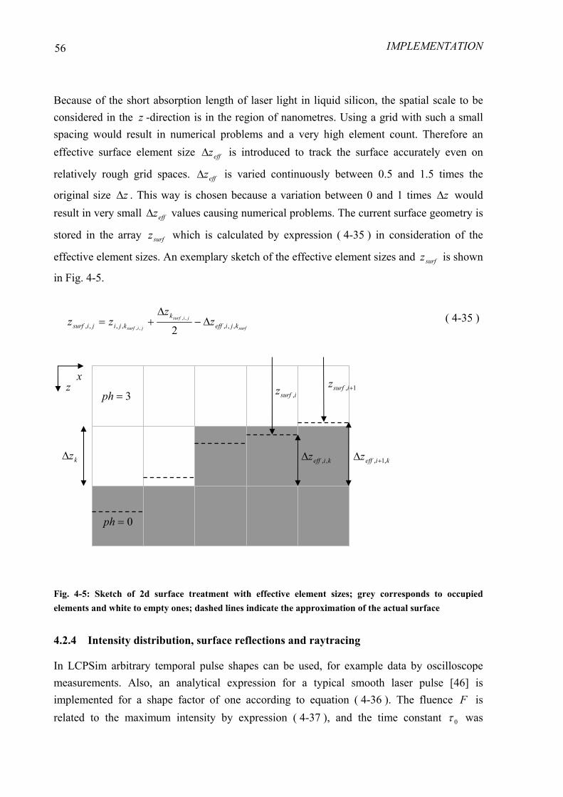
IMPLEMENTATION
56
Because of the short absorption length of laser light in liquid silicon, the spatial scale to be considered in the z -direction is in the region of nanometres. Using a grid with such a small spacing would result in numerical problems and a very high element count. Therefore an effective surface element size effzΔ is introduced to track the surface accurately even on
relatively rough grid spaces. effzΔ is varied continuously between 0.5 and 1.5 times the
original size zΔ . This way is chosen because a variation between 0 and 1 times zΔ would result in very small effzΔ values causing numerical problems. The current surface geometry is
stored in the array surfz which is calculated by expression ( 4-35 ) in consideration of the
effective element sizes. An exemplary sketch of the effective element sizes and surfz is shown
in Fig. 4-5.
surf
jisurf
jisurf kjieffk
kjijisurf zz
zz ,,,,,,, 2,,
,,Δ−
Δ+= ( 4-35 )
Fig. 4-5: Sketch of 2d surface treatment with effective element sizes; grey corresponds to occupied elements and white to empty ones; dashed lines indicate the approximation of the actual surface
4.2.4 Intensity distribution, surface reflections and raytracing
In LCPSim arbitrary temporal pulse shapes can be used, for example data by oscilloscope measurements. Also, an analytical expression for a typical smooth laser pulse [46] is implemented for a shape factor of one according to equation ( 4-36 ). The fluence F is related to the maximum intensity by expression ( 4-37 ), and the time constant 0τ was
x z
kzΔ kieffz ,,Δ
1, +isurfz isurfz ,
0=ph
3=ph
kieffz ,1, +Δ
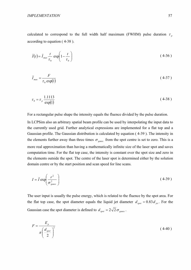
IMPLEMENTATION
57
calculated to correspond to the full width half maximum (FWHM) pulse duration pτ
according to equation ( 4-38 ).
( ) ⎟⎟⎠
⎞⎜⎜⎝
⎛−=
00
1expττttItI max ( 4-36 )
( )1exp0τFI max = ( 4-37 )
( )1exp1113.1
0 pττ = ( 4-38 )
For a rectangular pulse shape the intensity equals the fluence divided by the pulse duration.
In LCPSim also an arbitrary spatial beam profile can be used by interpolating the input data to the currently used grid. Further analytical expressions are implemented for a flat top and a Gaussian profile. The Gaussian distribution is calculated by equation ( 4-39 ). The intensity in the elements further away than three times gaussσ from the spot centre is set to zero. This is a
more real approximation than having a mathematically infinite size of the laser spot and saves computation time. For the flat top case, the intensity is constant over the spot size and zero in the elements outside the spot. The centre of the laser spot is determined either by the solution domain centre or by the start position and scan speed for line scans.
⎟⎟⎠
⎞⎜⎜⎝
⎛= 2
2
expgauss
rIIσ
( 4-39 )
The user input is usually the pulse energy, which is related to the fluence by the spot area. For the flat top case, the spot diameter equals the liquid jet diameter jetspot dd 83.0= . For the
Gaussian case the spot diameter is defined to gaussspotd σ22= .
2
2 ⎟⎟⎠
⎞⎜⎜⎝
⎛=
spot
p
d
EF
π
( 4-40 )

IMPLEMENTATION
58
If the average laser power P is given, the pulse energy is determined by the repetition rate
pf .
p
p fPE = ( 4-41 )
Before the laser light reaches the surface, absorption in the liquid jet is considered in LCPSim. For this the Lambert Beer law including the path enlargement is considered to calculate the intensity reaching the surface incI . Here the length of the liquid jet corresponds
to the working distance, i.e. nozzle outlet to original material surface.
( )( )surfjetsolvininc l zII +−= αδexp ( 4-42 )
For shallow ablation craters and grooves the laser light can be approximated to be perpendicular to the surface. Then the intensity coupled into the material is described by equations ( 2-16 ) and ( 2-10 ) applied to the surface elements. Thin film reflection is also implemented for perpendicular light. The equation ( 2-17 ) is optionally applied if the surface elements correspond to the original surface. Otherwise the thin film is assumed to be ablated and the standard reflectivity is used.
If the laser light can not be approximated to be perpendicular, a raytracing algorithm is implemented to account for multiple reflections and an angular dependent reflectivity. For this the slope of the surface geometry has to be determined. During the simulations, it has been observed that for stability reasons a special second order gradient scheme is best suitable for the 2d case. Here the gradient is calculated from the difference between slightly off centred values according to equation ( 4-43 ), illustrated in Fig. 4-6. This formulation shows a smoother slope and damps the developing of an observed numerical self focusing effect leading to tiny deep holes.
( )−+
−−−
−−−−−
+++
+++++
Δ+Δ+Δ
−
−Δ+−
−
−Δ+
=∇
xx
xx
xsurfxsurfxxsurf
xx
xsurfxsurfxxsurf
surf
xxx
xxzzx
zxxzzx
zz
65
33,,
,,,
,
( 4-43 )
From the gradient, the surface normal vector is calculated.

IMPLEMENTATION
59
( )( )( )( )⎟⎟⎠
⎞⎜⎜⎝
⎛
∇∇
= −
−
surf
surf
zz
n 1
1
tansintancos
( 4-44 )
Fig. 4-6: Illustration of smoothed surface slope and ray reflection for the 2d case
For the 3d case a regression plane is calculated using the eight surrounding surface points
jisurfz ,1, + , jisurfz ,1, − , 1,, +jisurfz , 1,, −jisurfz , 1,1, ++ jisurfz , 1,1, +− jisurfz , 1,1, −+ jisurfz and 1,1, −− jisurfz . The
corresponding formulas are taken from [58]. Taking into account eight rather than the minimum required four points has the same reasons for stability and accuracy as mentioned for the 2d case. Out of the plane equation the normal vector can be easily derived.
The incoming laser beam is divided into one discrete ray for every grid element in the x – y
plane with the corresponding intensity. To save computing time, the raytracing is performed only for elements where the intensity is greater than zero. The ray at ji, is assumed to be
directed in the positive z -coordinate. The total intensity of the ray is split into a parallel and a vertically polarized component. Every component has an initial value equal to the half of the total intensity 2|| incIII == ⊥ . The first reflection occurs at the surface element jisurfkji ,,,,
resulting in an arbitrary ray direction b calculated by equation ( 2-14 ). From this point the ray is traced by iteratively identifying the neighbouring element to which the ray travels. If the ray reaches a surface element, the ray direction changes again by reflection. The tracing is stopped if the ray reaches the solution domain boundary. If the mirror symmetry is applied, the y -component of the direction of a ray which reaches the mirror plane is changed in sign.
This reflected ray corresponds to the ray coming from the other side of the symmetry plane. In
x z
i
isurfz ,∇
n
linearly interpolated surface laser ray
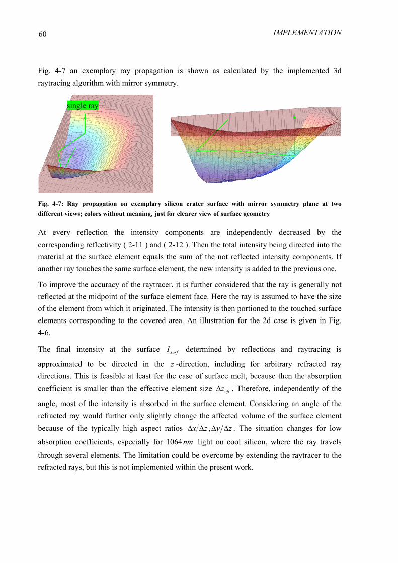
IMPLEMENTATION
60
Fig. 4-7 an exemplary ray propagation is shown as calculated by the implemented 3d raytracing algorithm with mirror symmetry.
Fig. 4-7: Ray propagation on exemplary silicon crater surface with mirror symmetry plane at two different views; colors without meaning, just for clearer view of surface geometry
At every reflection the intensity components are independently decreased by the corresponding reflectivity ( 2-11 ) and ( 2-12 ). Then the total intensity being directed into the material at the surface element equals the sum of the not reflected intensity components. If another ray touches the same surface element, the new intensity is added to the previous one.
To improve the accuracy of the raytracer, it is further considered that the ray is generally not reflected at the midpoint of the surface element face. Here the ray is assumed to have the size of the element from which it originated. The intensity is then portioned to the touched surface elements corresponding to the covered area. An illustration for the 2d case is given in Fig. 4-6.
The final intensity at the surface surfI determined by reflections and raytracing is
approximated to be directed in the z -direction, including for arbitrary refracted ray directions. This is feasible at least for the case of surface melt, because then the absorption coefficient is smaller than the effective element size effzΔ . Therefore, independently of the
angle, most of the intensity is absorbed in the surface element. Considering an angle of the refracted ray would further only slightly change the affected volume of the surface element because of the typically high aspect ratios zyzx ΔΔΔΔ , . The situation changes for low
absorption coefficients, especially for nm1064 light on cool silicon, where the ray travels
through several elements. The limitation could be overcome by extending the raytracer to the refracted rays, but this is not implemented within the present work.
single ray

IMPLEMENTATION
61
4.2.5 Semi analytical heat sources
Once the intensity at each surface element jisurfkjiI
,,,, is determined, the absorption equation
( 2-6 ) has to be solved. This is done by looping over the element column at ji, starting at the
surface element nzkk jisurf ..,,= . For every element the absorbed intensity is calculated and the
not absorbed part is given to the next element. The absorption coefficient is considered to be constant over one element, so the Lambert-Beer law can be applied. This gives a much more accurate solution than assuming a constant intensity over the element, in case the absorption coefficient is significantly smaller than the element size effzΔ . This is the case especially for
the surface elements, as illustrated in Fig. 4-8. Using equations ( 2-7 ) and ( 2-21 ) results in the intensity decrease ( 4-45 ) and heat source ( 4-46 ).
( )kjieffkjikjikji zII ,,,,,,,1,, exp Δ−=+ α ( 4-45 )
( )( )effeff
h zαzIS Δ−−
Δ= exp1 ( 4-46 )
Surface heat flux due to radiation ( 2-26 ) or heat transfer ( 2-27 ) is implemented for the ADE method by heat source terms in the surface elements. The corresponding heat sink is generally calculated by expression ( 4-47 )
jisurf
jisurf
jisurfkjieff
kjisurfkjih z
JS
,,
,,
,,,,,
,,,,,, Δ
−= ( 4-47 )
4.2.6 Surface recession due to evaporation
For both evaporation models the latent heat of evaporation is a decisive factor. In LCPSim no density changes are considered, therefore equation ( 2-30 ) is applied using the density of liquid silicon at the melting point of lkg54.2 , which results in ³286.36 mmJLv = .
For the enthalpy based evaporation, a semi analytical model is used where the enthalpy distribution in the z -direction of the surface elements is not treated as a constant value but calculated by analytical equations. This gives a more accurate solution of the evaporation speed and of the average enthalpy in the surface elements, including for rather large element sizes. This model has been published in [57] and was further improved within the present work. During evaporation the enthalpy distribution near the surface is dominated by the heat
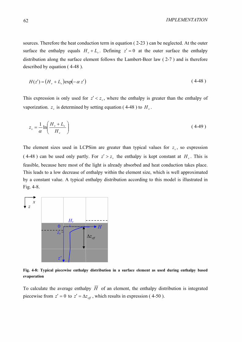
IMPLEMENTATION
62
sources. Therefore the heat conduction term in equation ( 2-23 ) can be neglected. At the outer surface the enthalpy equals vv LH + . Defining 0=′z at the outer surface the enthalpy
distribution along the surface element follows the Lambert-Beer law ( 2-7 ) and is therefore described by equation ( 4-48 ).
( ) ( )zLHzH vv ′−+=′ αexp)( ( 4-48 )
This expression is only used for vzz <′ , where the enthalpy is greater than the enthalpy of
vaporization. vz is determined by setting equation ( 4-48 ) to vH .
⎟⎟⎠
⎞⎜⎜⎝
⎛ +=
v
vvv H
LHz ln1
α ( 4-49 )
The element sizes used in LCPSim are greater than typical values for vz , so expression
( 4-48 ) can be used only partly. For vzz >′ the enthalpy is kept constant at vH . This is
feasible, because here most of the light is already absorbed and heat conduction takes place. This leads to a low decrease of enthalpy within the element size, which is well approximated by a constant value. A typical enthalpy distribution according to this model is illustrated in Fig. 4-8.
Fig. 4-8: Typical piecewise enthalpy distribution in a surface element as used during enthalpy based evaporation
To calculate the average enthalpy H of an element, the enthalpy distribution is integrated piecewise from 0=′z to effzz Δ=′ , which results in expression ( 4-50 ).
x z
effzΔ
HHv
z'
zv
0

IMPLEMENTATION
63
( )( ) vvv
vvH
eff
Hv
zHzLH
C
zCHH
−−−+
=
Δ+=
αα
exp1 ( 4-50 )
If the average enthalpy nH is above the vaporization point vH and increases during one time
step about HΔ the surface element size is reduced due to evaporation. The new effective
element size 1+Δ neffz and the new average enthalpy 1+nH are then derived from the energy
balance ( 4-51 ) to the formulas ( 4-52 ) and ( 4-53 ).
( )( ) ( ) neff
nneff
nvv
neff
neff zHHzHLHzz ΔΔ+=Δ++Δ−Δ +++ 111 ( 4-51 )
( )
v
Hn
vvneffn
eff LCHHLHz
z+Δ−−+Δ
=Δ +1 ( 4-52 )
11
++
Δ+= n
eff
Hv
n
zC
HH ( 4-53 )
Note that this model is only applied during evaporation for positive enthalpy changes. After evaporation, i.e. if the average enthalpy falls below vH , the enthalpy is again assumed to be
equally distributed over the effective element size.
For the Knudsen evaporation no similar semi analytical model has been derived, because the equations are more complex than can be solved analytically. Due to the negative surface heat flux by the latent heat, the outer surface is not necessarily hotter than the average element temperature. Therefore the assumption of an equally distributed enthalpy in the surface elements is a better approximation than in the case of enthalpy based evaporation.
The change of the effective element size within the Knudsen model is calculated by the evaporation velocity ( 2-33 ) and the current time step according to equation ( 4-54 ). The surface heat flux is considered by updating the current element enthalpy corresponding to the latent heat of the evaporated volume, see equation ( 4-55 ).
tvzz lvneff
neff Δ−Δ=Δ +1 ( 4-54 )

IMPLEMENTATION
64
( ) vneff
neff
nn LzzHH 111 +++ Δ−Δ−= ( 4-55 )
Note that for the Knudsen evaporation the time step has to be restricted as discussed before according to equation ( 4-20 ).
If the element size kjieffz ,,,Δ falls below 2,, kjizΔ during one time step, the element is
assumed to be fully evaporated by setting 3,, =kjiph . The underlying element in the positive
z -direction is treated as the new surface element. For conservation of mass and energy the element size and the average enthalpy of the underlying element have to be updated according to equations ( 4-56 ) and ( 4-57 ).
kjieffkkjieff zzz ,,,11,,, Δ+Δ=Δ ++ ( 4-56 )
1,,,
,,,,,1,,11,,
+
+++ Δ
Δ+Δ=
kjieff
kjikjieffkjikkji z
HzHzH ( 4-57 )
Because the effective surface element sizes are independently calculated, neighbouring surface elements in the x - and y -directions have generally different element sizes. Therefore
the heat flux between two neighbouring elements is adjusted by the minimum of both element sizes. An example for the positive x -direction is given in equation ( 4-58 ).
( )
k
kjieffkjieffkjikjieff z
zzJJ
Δ
ΔΔ= +
++,,1,,,,
,,5.0,,5.0,
,min ( 4-58 )
4.2.7 Diffusion of impurity atoms in silicon melt
The diffusion coefficient of impurity atoms in silicon melt can be approximated by a constant value as discussed in section 2.3.4. Furthermore, no melt movement is considered in LCPSim, therefore Fick’s Law ( 2-37 ) can be applied. The implementation is done in the same way for the concentration C as described in section 4.2.1 for the enthalpy H . The resulting finite differences expressions, shown in equation ( 4-59 ) for 2d axial symmetry, are much simpler.

IMPLEMENTATION
65
⎟⎟⎟⎟
⎠
⎞
⎜⎜⎜⎜
⎝
⎛
Δ−−
−−−
+Δ
−−
−−−
= −
−
+
+
−
−−
+
++
zzzCC
zzCC
xrxxCC
rxxCC
rC z
z
z
z
x
xx
x
xx
Ddtd 5.05.0
( 4-59 )
If diffusion is switched on in LCPSim, for every element two equations, heat transport and dopant diffusion, have to be numerically integrated. For the implicit methods and the ADE method this is done in a segregated way by first solving for the enthalpy and afterwards for the concentration. This is reasonable because the dopant concentration does not influence the heat transport equation. The ADE implementation is done according to section 4.2.2. The same time step size can be used as for the single heat transport time integration, because the diffusion occurs on significantly greater time scales than the heat transport. Therefore no error is introduced by way of insufficiently large time step size.
Similar to the heat transport equation, a non isolating boundary condition at the surface is implemented by a dopant source term. It is determined by the surface concentration according to equation ( 4-60 ).
2,,,
,,,,,,,,
,,
,,,,
,,
jisurf
jisurfjisurf
jisurfkjieff
kjikjisurfkjisp z
CCDS
Δ
−= ( 4-60 )
For the infinite source boundary condition the surface concentration surfC is set to a constant
value. In the case of the finite source boundary condition the decrease of loading over time has to be considered. For this a loading array ji ,Θ is used where values are updated after
every time step according to expression ( 4-61 ). The current surface concentration is then calculated by equation ( 2-40 ).
jisurf
jisurfjisurf
kjieff
kjikjisurfnji
nji z
CCDt
,,
,,,,
,,,
,,,,,,
1, Δ
−Δ−Θ=Θ + ( 4-61 )
In the solid silicon region the concentration change is set to zero because the solid state diffusion is neglected as discussed in section 2.3.4. To hinder a numerical dopant sink at the solid – liquid interface, an isolating boundary condition is applied. This is done in a similar way as for the surface boundary conditions. Equation ( 4-62 ) gives an example for the positive z -direction.

IMPLEMENTATION
66
( )( )++++ −≤∩>+= zzzz CCphphCC 5.05.0 ( 4-62 )
A special analyzing feature was implemented in LCPSim to get the doping profile in a way that corresponds to the secondary ion mass spectroscopy (SIMS) measurement technique. Here the ion beam targeting on the sample has a diameter of usually greater than µm10 and
gives therefore a doping profile which is averaged over the spot size. In LCPSim a corresponding algorithm was implemented which performs the averaging of the concentration over a defined spot size. It also considers an arbitrary surface geometry as illustrated in Fig. 4-9. The program code is given in A.4.
Fig. 4-9: Illustration of SIMS method as implemented in LCPSim
4.2.8 Multilayer implementation
LCPSim focuses on silicon processing, but the code is basically able to calculate other materials by adjusting the material properties. Furthermore, a multilayer implementation was performed to simulate multiple layers of materials. This is done by introducing a VOF model similar to the fluid flow multiphase model described in section 2.4.2. For each material a volume fraction array a is assigned. The material properties, namely the enthalpy – temperature relation and the optical properties, are calculated in every time step according to equation ( 2-45 ). Also, the constant material properties like the latent heat are stored in arrays assigned to the actual material property. The time integration is then performed on the mixture level.
In LCPSim up to three layers with time independent interfaces at user defined z -values can be applied, see Fig. 4-10. The element faces are ensured to fit exactly the interface position. In
ion beam diameter
averaged region groove cross section

IMPLEMENTATION
67
this way, in no element are different materials shared. Especially the piecewise defined temperature – enthalpy relation can then be directly applied instead of having a more complex formulation for mixed elements. This actually is no restriction, because no flow, i.e. change of the material distribution over time, is considered in LCPSim.
Fig. 4-10: Exemplary material distribution for three layers as used in LCPSim
For the upper layer the thin film reflectivity ( 2-17 ) is implemented for optional use and takes into account the current thickness of the layer.
Within this work only a 2d solver for the multilayer model is implemented. An implementation in 3d would be quite straight forward, but was not done within the timeframe of the present work.
4.2.9 Grid generation and adaptation
Besides the ADE implementation, an adaptive grid possesses great potential to reduce the computing time compared to an overall fine grid. Laser processing shows large differences in spatial scales. For example, doping has to be calculated on the scale of several tens of nanometers, whereas the solution domain should be several hundred micrometers. Therefore adapting the grid to the regions of interest greatly reduces the overall element count.
The grid adaptation is applied in every time step. The basic strategy differs between the pulse and the pulse pause, which is typically many times longer than the pulse. During the pulse a finer grid is used, which is stored at the point of full solidification. Also, the dopant distribution is stored because it does not change during the pulse pause. After solidification a much coarser grid is allowed as well with a coarsening of the surface geometry. This increases the possible time step size and reduces the element count, resulting in highly
material 1
0,0,1 321 === aaa
x z
material 2
0,1,0 321 === aaa
material 3
1,0,0 321 === aaa
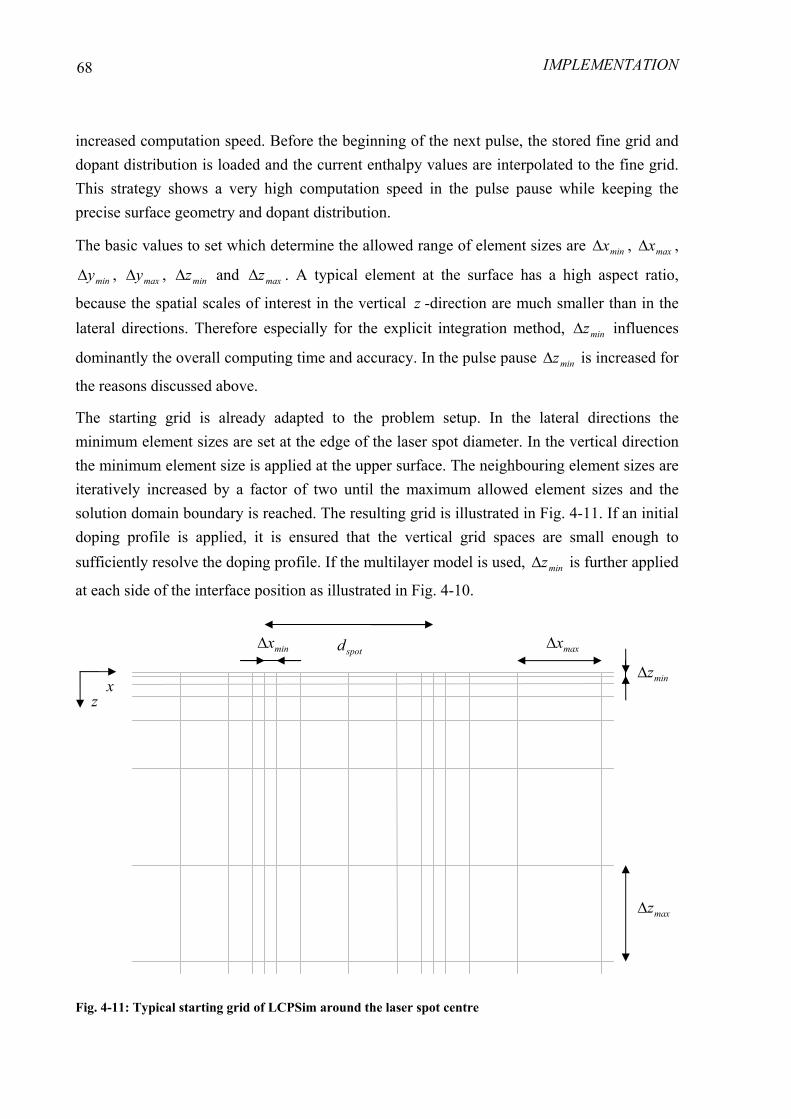
IMPLEMENTATION
68
increased computation speed. Before the beginning of the next pulse, the stored fine grid and dopant distribution is loaded and the current enthalpy values are interpolated to the fine grid. This strategy shows a very high computation speed in the pulse pause while keeping the precise surface geometry and dopant distribution.
The basic values to set which determine the allowed range of element sizes are minxΔ , maxxΔ ,
minyΔ , maxyΔ , minzΔ and maxzΔ . A typical element at the surface has a high aspect ratio,
because the spatial scales of interest in the vertical z -direction are much smaller than in the lateral directions. Therefore especially for the explicit integration method, minzΔ influences
dominantly the overall computing time and accuracy. In the pulse pause minzΔ is increased for
the reasons discussed above.
The starting grid is already adapted to the problem setup. In the lateral directions the minimum element sizes are set at the edge of the laser spot diameter. In the vertical direction the minimum element size is applied at the upper surface. The neighbouring element sizes are iteratively increased by a factor of two until the maximum allowed element sizes and the solution domain boundary is reached. The resulting grid is illustrated in Fig. 4-11. If an initial doping profile is applied, it is ensured that the vertical grid spaces are small enough to sufficiently resolve the doping profile. If the multilayer model is used, minzΔ is further applied
at each side of the interface position as illustrated in Fig. 4-10.
Fig. 4-11: Typical starting grid of LCPSim around the laser spot centre
minzΔ
maxzΔ
minxΔ maxxΔ
x z
spotd

IMPLEMENTATION
69
The adaption algorithm checks the enthalpy, heat source and concentration differences between neighbouring elements. If they are above a critical value, the elements are considered for refinement, and if they are below another critical value they are considered for coarsening. Because of the structured grid the adaption is applied to an element row for 2d and an element plane for 3d. The algorithm is explained in the following for the element sizes in the z -direction for the 2d case.
For every kz -value, the maximum difference to the neighbouring elements is evaluated
according to expression ( 4-63 ) for the enthalpy case. This is done in the same way for the heat source and concentration.
( )1,,..1, max += −=Δ kikinxikmax HHH ( 4-63 )
If one difference is above the critical value, critmax HH Δ>Δ or crithmaxh SS ,, Δ>Δ or
critmax CC Δ>Δ , and if the element size kzΔ is greater than two times minzΔ , a refinement step
is performed for both rows at k and 1+k in the same way. The element size is divided in such a way that the new size is not greater than the neighbouring element size in the negative z -direction, see expressions ( 4-64 ) and ( 4-65 ) for the 1+k row. The reason for this is that typically the gradients to be resolved increase for decreasing distance to the surface affected by the laser.
⎟⎠⎞
⎜⎝⎛ ΔΔ
=Δ ++ k
knewk z
zz ,
2min 1
,1 ( 4-64 )
newkknewk zzz ,11,2 +++ Δ−Δ=Δ ( 4-65 )
Once the element sizes are determined, values for enthalpy and concentration have to be assigned to the new elements. For the concentration, simply the value of the old elements is assigned. For the enthalpy a more accurate interpolation is applied. Here the slope of the enthalpy between the elements k and 1+k is used to set the new enthalpy values according to equations ( 4-66 ) to ( 4-68 ). This formulation ensures conservation of energy and gives a better approximation to the actual enthalpy distribution.
kk
kikiki zz
HHH
−
−=∇
+
++
1
,1,5.0, ( 4-66 )

IMPLEMENTATION
70
2
,25.0,1,,1,
newkkikinewki
zHHH +
+++
Δ∇−= ( 4-67 )
2
,15.0,1,,2,
newkkikinewki
zHHH +
+++
Δ∇+= ( 4-68 )
If all differences for enthalpy, heat source and concentration are below a critical value, the element rows k and 1+k are considered for coarsening. Several restrictions for coarsening are implemented. At the beginning of the laser pulse no coarsening is allowed to ensure “catching” of the laser spot with a suitable grid. Merging of surface elements with empty elements is not allowed during the pulse. During the pulse pause it is allowed, but only to a certain amount to keep roughly the surface geometry. Furthermore, the merged element size must be smaller than two times the neighbouring element sizes and smaller than maxzΔ . For
the explicit time integration methods, a coarsening step is performed only once for every 50 time steps. This is done to hinder grid oscillations as observed for small time step sizes. For the implicit and ADE methods, in every second time step coarsening was shown to be practical.
If all restrictions are checked, the element rows or planes are merged. The enthalpy and concentration values are calculated by size weighted averages according to equation ( 4-70 ) for the enthalpy case.
1, +Δ+Δ=Δ kknewk zzz ( 4-69 )
newk
kkikkinewki z
zHzHH
,
11,,,1, Δ
Δ+Δ= ++
+ ( 4-70 )
The same algorithm is performed for the lateral coordinate directions. The only difference is that the enthalpy is equally distributed during a refinement step, rather than using the slope method described above. This is because especially for flat top laser profiles, quite sharp jumps of enthalpy are observed in the lateral direction. Therefore the approximation of a continuous slope of enthalpy is bad and leads to numerical problems.
The programming of a consistent and stable adaption algorithm was not straightforward, especially because of the arbitrary surface geometry and the coarsening of the surface

IMPLEMENTATION
71
geometry during the pulse pause. Care had to be taken to the looping orders and to ensure consideration of all rows to be refined. For more details the program code is given in A.2.
The refinement and coarsening thresholds of enthalpy, source and concentration were derived empirically by comparing the simulation results for different settings. A good choice for the
refinement thresholds was observed to be ³2 15, mWeS crith =Δ , ³5 8 mJeH crit =Δ and
3183 −=Δ meCcrit . The coarsening thresholds are set to 0.3 times the refinement thresholds.
4.2.10 User settings and program structure
A rudimentary text based user interface is implemented by summarizing all parameters and other applicable settings like graphical output into one file named start.m. Each temperature dependent material property is set in an extra file, because this file has to be loaded during every time step. The constant material properties and the parameters for the temperature – enthalpy relation are set in one extra file. For the multilayer simulation, separate files for each material are used.
An example for the file start.m can be looked up in A.1. In the first section the models to be considered can be switched. This is namely 2d or 3d with corresponding symmetries, dopant diffusion, evaporation model, raytracing and laser type. The laser type is either a dry laser or LCP, where the latter takes into account absorption in the liquid jet and the pressure induced by the liquid jet impingement on a flat surface. The next section provides settings for the laser parameters like wavelength, pulse duration, spot diameter etc. In case of diffusion switched on, an initial doping profile from a data file and the parameters for the boundary conditions can be applied. Furthermore, the dimensions of the solution domain and the grid adaptation parameters are set. The time integration method can be switched between the implemented models for the evaporation and non evaporation regime independently. The simulation time is the physical time the simulation will run, determined either by the time span itself, the scan length or the number of pulses.
A flexible function for graphical output has been programmed, which is controlled also by settings in start.m. Basically a figure with four axes is plotted, where every plot can be defined independently. Predefined surface and curve plots are assigned by a number for each axis. For every plot the axis scales can be set, otherwise the whole solution domain is plotted. Multiple curves can be plotted on one axis by assigning multiple numbers to one plot. Next, the cut coordinates and the surface plot direction are set to determine the position and orientation of the plots in the solution domain. The graphical output is performed at defined time intervals during the simulation, where also the current grid and solution values are stored. Optionally, videos of each axis can be stored with the frames corresponding to the

IMPLEMENTATION
72
output time intervals. An exemplary output of a 3d simulation including dopant diffusion is given in Fig. 4-12.
Fig. 4-12: Exemplary output of LCPSim corresponding the settings of start.m as shown in A.1
At the end of start.m a parameter sweep is implemented. Here any parameter defined above can be used for sweeping and the results are automatically stored in separate folders. For a better understanding of LCPSim a program flow chart is shown in Fig. 4-13 for the standard ADE solver.

IMPLEMENTATION
73
Fig. 4-13: Program flow chart of LCPSim for the case of the ADE solver
4.2.11 Verification
To verify the basic solver for the heat transport equation, an analytic solution for a simplified case is derived. Assuming time and spatially independent constant laser intensity, a one dimensional steady state problem with a constant surface recession speed lvv is achieved. For
a moving frame of reference with 0=z fixed at the surface, the heat transport equation can be expressed by equation ( 4-71 ). In addition, a constant absorption coefficient and heat conductivity are assumed here.
( )zIdzdHv
dzHd
cK
surflvp
ααρ
−++= exp0 2
2
( 4-71 )
For enthalpy based evaporation the surface recession speed is given by vsurflv LIv = , and the
enthalpy value at the surface equals the sum of the enthalpy of vaporization and the latent heat of vaporization, ( ) vv LHzH +== 0 . In a defined region vzz < , the enthalpy is above vH
and the temperature is constant at the vaporization temperature. Therefore the heat conduction term can be neglected. This gives a simple exponential solution of equation ( 4-71 ).
tCH nn ,,
11 , ++ nn CH

IMPLEMENTATION
74
( ) ( ) ( )zLHzzH vvv α−+=< exp ( 4-72 )
This expression is equal to equation ( 4-48 ), therefore vz is calculated according to equation
( 4-49 ). For vzz > the solution is given by the sum of two exponential functions.
( ) ( ) ( ) ( ) ( )( )
( )
surfpvv
v
vvvv
surfpvv
IcK
LH
zC
zzCzzLHK
IcCHzzH
ρα
α
αρ
−+
−=
−−+⎟⎟⎠
⎞⎜⎜⎝
⎛−
+−−=>
1exp
expexp
1
11
( 4-73 )
In Fig. 4-14 the comparison of 2d simulation results and the analytical solution is shown. The laser spot diameter in the simulation is chosen high enough to ensure that no lateral effects influence the enthalpy distribution at the laser spot centre. Typical properties for liquid silicon
are used with 161 −= cmeα and KmWK 70= . A very good agreement can be seen, proving
the correct implementation and a good numerical accuracy of the basic code for different grid sizes as well. Note that the symbols left of the sharp bend at vzz = do not correspond to
element centres, but are calculated by equation ( 4-72 ) for illustration of the semianalytical enthalpy distribution.
0 0.2 0.4 0.6 0.8 1 1.20
2
4
6
8
10
12
14
16
18
20
distance to surface [µm]
enth
alpy
[J/m
m³]
analytic solutionsimulation, Δzmin = 50 nmsimulation, Δzmin = 20 nm
Fig. 4-14: Comparison of analytic solution and simulation results for two different grid settings and a not reflected laser intensity of 55 MW/cm²; dotted line corresponds to the onset of solid – liquid phase change
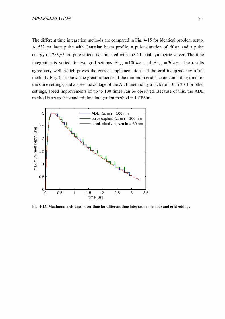
IMPLEMENTATION
75
The different time integration methods are compared in Fig. 4-15 for identical problem setup. A nm532 laser pulse with Gaussian beam profile, a pulse duration of ns50 and a pulse
energy of µJ283 on pure silicon is simulated with the 2d axial symmetric solver. The time
integration is varied for two grid settings nmzmin 100=Δ and nmzmin 30=Δ . The results
agree very well, which proves the correct implementation and the grid independency of all methods. Fig. 4-16 shows the great influence of the minimum grid size on computing time for the same settings, and a speed advantage of the ADE method by a factor of 10 to 20. For other settings, speed improvements of up to 100 times can be observed. Because of this, the ADE method is set as the standard time integration method in LCPSim.
0 0.5 1 1.5 2 2.5 3 3.50
0.5
1
1.5
2
2.5
3
time [µs]
max
imum
mel
t dep
th [µ
m]
ADE, Δzmin = 100 nmeuler explicit, Δzmin = 100 nmcrank nicolson, Δzmin = 30 nm
Fig. 4-15: Maximum melt depth over time for different time integration methods and grid settings

IMPLEMENTATION
76
0 20 40 60 80 100 12010
0
101
102
103
minimum element size [nm]
com
putin
g tim
e [m
in]
euler explicitcrank nicolsonADE
Fig. 4-16: Dependency between computing time and grid size for different time integration methods for a typical laser pulse
Further verification is done by reproducing measured and calculated melt durations presented by Lowndes et al. [59]. One simulation was performed using the optical properties suggested in [59], mainly a constant reflectivity of 0.7 of molten silicon, and the other one with the models as described in this work. A second set of measurements is shown as derived from [60]. The results in Fig. 4-17 show a good agreement with the data of Lowndes et al., using the reported settings. For the standard settings, the simulation is still well within the measured data. The differences between the curves near the melting threshold could be due to different grids used, because here the melt depth is smaller than the minimum element size of LCPSim. This is also the reason for the step at roughly nm20 , where the surface element is fully
molten.

IMPLEMENTATION
77
0 0.2 0.4 0.6 0.8 1 1.20
0.02
0.04
0.06
0.08
0.1
0.12
0.14
fluence [J/cm²]
mel
t dur
atio
n [µ
s]
Auston et. al. (smoothed)Lowndes et. al.LCPSim, settings according to Lowndes et. al.LCPSim, standard settings
Fig. 4-17: Comparison of simulation results with measured data from literature, [59] and [60]
To verify the implementation of the diffusion equation, the phosphorous diffusion by an unlimited source in silicon melt was simulated and compared with the analytical solution ( 4-74 ). The results by the analytical solution and the ADE solver in Fig. 4-18 show excellent agreement and prove the correct implementation off the diffusion equation in LCPSim.
( )⎟⎟
⎠
⎞
⎜⎜
⎝
⎛⎟⎟⎠
⎞⎜⎜⎝
⎛−=
tD2zerf1surfCzC ( 4-74 )
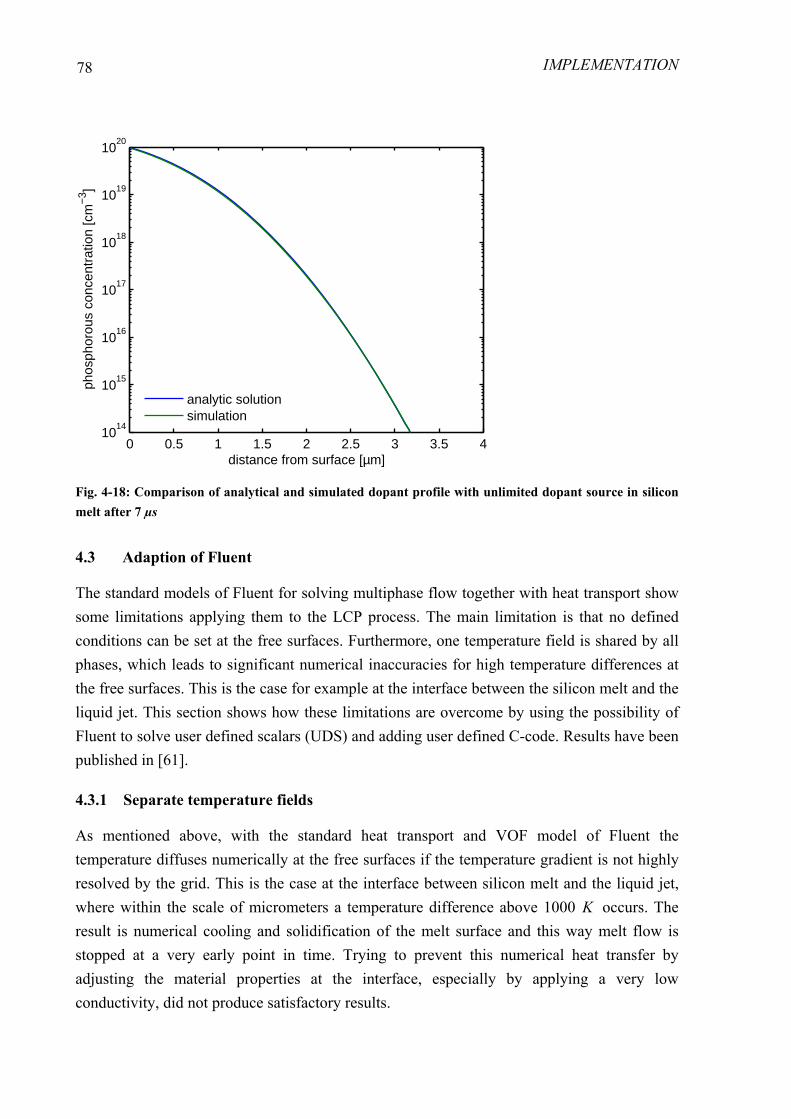
IMPLEMENTATION
78
0 0.5 1 1.5 2 2.5 3 3.5 410
14
1015
1016
1017
1018
1019
1020
distance from surface [µm]
phos
phor
ous
conc
entr
atio
n [c
m−
3 ]
analytic solutionsimulation
Fig. 4-18: Comparison of analytical and simulated dopant profile with unlimited dopant source in silicon melt after 7 µs
4.3 Adaption of Fluent
The standard models of Fluent for solving multiphase flow together with heat transport show some limitations applying them to the LCP process. The main limitation is that no defined conditions can be set at the free surfaces. Furthermore, one temperature field is shared by all phases, which leads to significant numerical inaccuracies for high temperature differences at the free surfaces. This is the case for example at the interface between the silicon melt and the liquid jet. This section shows how these limitations are overcome by using the possibility of Fluent to solve user defined scalars (UDS) and adding user defined C-code. Results have been published in [61].
4.3.1 Separate temperature fields
As mentioned above, with the standard heat transport and VOF model of Fluent the temperature diffuses numerically at the free surfaces if the temperature gradient is not highly resolved by the grid. This is the case at the interface between silicon melt and the liquid jet, where within the scale of micrometers a temperature difference above 1000 K occurs. The result is numerical cooling and solidification of the melt surface and this way melt flow is stopped at a very early point in time. Trying to prevent this numerical heat transfer by adjusting the material properties at the interface, especially by applying a very low conductivity, did not produce satisfactory results.
IMPLEMENTATION
79
To solve this problem, one UDS for each phase corresponding to the temperature of the regarding phase is applied. As discussed in section 3.2.2, this ensures that the temperature is conserved within the phase boundaries, including for large differences between the separate temperature fields. For solving the heat transport equation ( 2-20 ) by the UDS equation ( 3-18 ), the general diffusivity has to be set to pcK=Γ and the heat sources have to be
divided by the heat capacity. A diffusivity – UDF is used for adjusting the temperature dependent diffusivity during each iteration.
The UDS under relaxation factor in Fluent has to be set to 0.9, which has been observed to be a suitable value for good convergence behaviour.
4.3.2 Melting / solidification and density change
In Fluent a melting / solidification model is implemented by an enthalpy based phase change approach. However, it requires the standard temperature to be solved, which is not the case if separate temperature fields via UDS are solved instead. Therefore the melting solidification model is additionally implemented by UDF using the silicon UDS temperature field. For this a momentum source UDF for radial and axial momentum is applied according to equations ( 2-47 ) and ( 2-48 ), using the UDS for the silicon phase rather than the standard Fluent temperature. For a fast convergence and numerical stability, and also for relatively large time step sizes, it is important to assign also the derivative of the momentum sources according to equation ( 4-75 ). This user defined melting / solidification model, combined with the UDS temperature fields, is numerically not as stable as the standard models. Especially a high grid quality is required to hinder inaccuracies and divergence of the pressure field at the free surface. Therefore in this work only rectangular structured grids are used in the region of the free surface.
( ) 53
2
1001.0
1 edv
dSmom
+−
=β
β ( 4-75 )
If heat transport is simulated in Fluent by UDS temperature fields, the latent heat of melting has to be considered during the phase change. This is done by implementing a user defined source to the UDS. The phase change takes place within a defined temperature interval mTΔ
as mentioned in section 2.4.3. If during one time step the temperature change of an element nn TTT −=Δ +1 intersects with this phase change interval, the latent heat has to be partly
released as a heat source according to the amount of intersection. The simplest formulation is to use an equally distributed temperature specific latent heat as illustrated in Fig. 4-19. The absolute latent heat to be applied is calculated by the integral over the intersected temperature
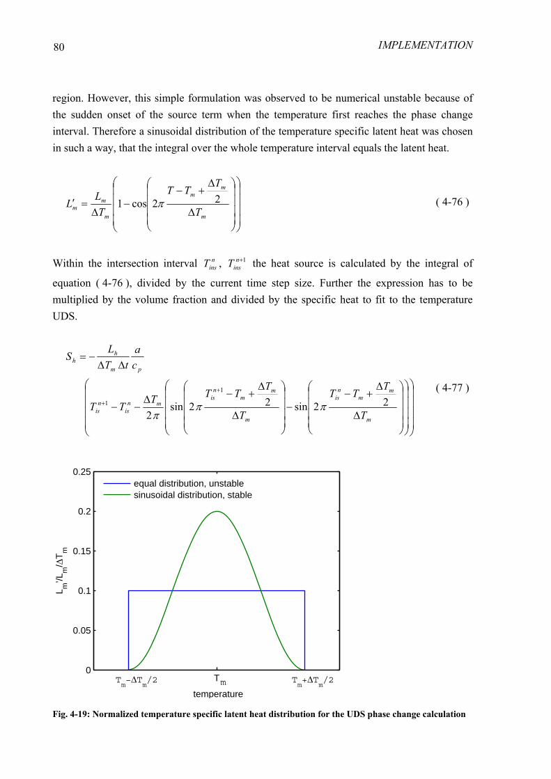
IMPLEMENTATION
80
region. However, this simple formulation was observed to be numerical unstable because of the sudden onset of the source term when the temperature first reaches the phase change interval. Therefore a sinusoidal distribution of the temperature specific latent heat was chosen in such a way, that the integral over the whole temperature interval equals the latent heat.
⎟⎟⎟⎟
⎠
⎞
⎜⎜⎜⎜
⎝
⎛
⎟⎟⎟⎟
⎠
⎞
⎜⎜⎜⎜
⎝
⎛
Δ
Δ+−
−Δ
=′m
mm
m
mm T
TTT
TL
L 22cos1 π ( 4-76 )
Within the intersection interval ninsT , 1+n
insT the heat source is calculated by the integral of
equation ( 4-76 ), divided by the current time step size. Further the expression has to be multiplied by the volume fraction and divided by the specific heat to fit to the temperature UDS.
⎟⎟⎟⎟
⎠
⎞
⎜⎜⎜⎜
⎝
⎛
⎟⎟⎟⎟
⎠
⎞
⎜⎜⎜⎜
⎝
⎛
⎟⎟⎟⎟
⎠
⎞
⎜⎜⎜⎜
⎝
⎛
Δ
Δ+−
−⎟⎟⎟⎟
⎠
⎞
⎜⎜⎜⎜
⎝
⎛
Δ
Δ+−Δ
−−
ΔΔ−=
+
+
m
mm
nis
m
mm
nis
mnis
nis
pm
hh
T
TTT
T
TTTT
TT
ca
tTL
S
22sin22sin2
1
1 πππ
( 4-77 )
T0
0.05
0.1
0.15
0.2
0.25
temperature
L m’/L
m/Δ
Tm
equal distribution, unstablesinusoidal distribution, stable
Tm−ΔT
m/2 T
m+ΔT
m/2m
Fig. 4-19: Normalized temperature specific latent heat distribution for the UDS phase change calculation

IMPLEMENTATION
81
Fluent is able to consider temperature dependent density changes within incompressible flow when solving of the temperature. Using the UDS temperature fields, the adjusting of the density is also done by Fluent but no volume change is calculated. This corresponds to a numerical mass source which is compensated by a UDF mass sink according to expression ( 4-78 ).
t
Snn
mass Δ−
−=+ ρρ 1
( 4-78 )
4.3.3 Free surface heat transfer
Introducing the independent temperature fields results in no heat transfer between the phases. To consider physical heat transfer without numerical diffusion, the model according to Fig. 2-9 is applied to the free surface between solid or molten silicon and the liquid media. This is possible, because the liquid side temperature gradient is satisfactorily resolved by a typically used grid. To apply equation ( 2-28 ), the directional derivative of the liquid side temperature has to be evaluated. Additionally, the heat flux has to be multiplied by the surface area density, i.e. the surface area per volume, to yield heat source terms that can be given to Fluent. The implemented algorithm for the free surface heat transfer model is explained in the following.
A loop over all faces of the current element is performed to identify the neighbouring elements. The element is treated as a surface element, if the liquid volume fraction is greater than 0.53 and at least one neighbouring element shows a silicon volume fraction greater than 0.47. Then the face with the highest scalar product of volume fraction gradient and face are
vector ( ) faceface aA ∇⋅ is determined to identify the neighbouring element located closest in
the direction of the surface normal. The surface is now approximated to be located parallel to the element face, which ends up in the situation illustrated in Fig. 4-20 for a 2d rectangular grid.

IMPLEMENTATION
82
Fig. 4-20: Sketch of approximated volume fraction and temperature distribution at the phase interface
The temperature of the surface is approximated to equal the temperature of the silicon in the neighbouring element and the liquid temperature is defined in the centre of the current element. For calculating the liquid side temperature gradient, the distance between surface and current element centre has to be used, which is calculated by the volume fractions according to the denominator in expression ( 4-79 ). Here it is further considered that the actual distance is decreased if the face normal is not in the direction of the surface normal by using the scalar product of the normalized vectors. To hinder a zero denominator, the liquid volume fraction has to be greater than 0.5, which explains the threshold value of 0.53 as mentioned above.
( ) ( ) ( ) ( )normnormliquidnbliquidnbnb
liquidnbsilicon
aAaayyxx
TT
nddT
∇⋅−+−+−
−=
5.0,22
, ( 4-79 )
For calculation of the heat sources, expression ( 4-79 ) has to be multiplied by the liquid heat conductivity and the surface area density, which equals the norm of the volume fraction
gradient a∇ . For numerical reasons, the volume fraction gradient is not one element sharp
but is spread over the neighbours of the element containing the actual interface. Therefore the volume fraction gradient of the current and the neighbouring element is added, which has been observed to approximate the real surface area density satisfactorily. The heat source term for the liquid temperature field is then given by equation ( 4-80 ). For the silicon temperature field, the heat source is applied to the neighbouring element and has to be adjusted by the element volumes to ensure conservation of energy.
liquid silicon
neighbouring element current element
possible interface location
elem
ent f
ace
temperature
IMPLEMENTATION
83
( )nbliquidliquidh aa
nddTKS ∇+∇=, ( 4-80 )
nb
liquidhnbsiliconh VVSS ,,, = ( 4-81 )
The algorithm is implemented by source UDFs and is applied within Fluent to the UDS temperature fields. Details can be looked up in A.4.
The basic algorithm for the interfacial heat transfer can be also adapted to arbitrary interfacial models like mass transfer due to surface reactions or diffusion, which is not possible with the standard models of Fluent.
4.3.4 Verification
Even in the very small spatial and temporal scales of LCP Fluent produces accurate simulation results for the basic fluid flow. This can be derived from published simulation results for similar scales. For example in [62] the liquid jet generation in different nozzles comparable to the LCP setup was succesfully simulated by Fluent.
To verify the free surface heat transfer between the UDS temperature fields a steady test case was simulated. A jet impingingment on silicon with a slightly angled surface and a constant temperature of K1000 is calculated in such a way that the height difference of the surface at
the outer solution domain boundaries is in the range of several element depths. This way the heat transfer is calculated for different volume fractions of water at the surface elements. As a reference, the jet impingement on an even wall with a temperature of K1000 is simulated
using the standard heat transport model of Fluent. The axial symmetric simulation setups are illustrated in Fig. 4-21. In both setups a µm50 wide water jet with a velocity of roughly
sm150 is used. The minimum grid size of the rectangular grid region as illustrated in Fig.
4-27 is nm100 in axial and nm250 in radial direction.

IMPLEMENTATION
84
Fig. 4-21: Jet impingement setups for heat transfer calculations; Left: reference setup for Fluent’s standard temperature model; Right: slightly angeled silicon surface within the solution domain for UDS temperature fields and UDF surface heat transfer
The calculated heat transfer coefficients at the surface are compared in Fig. 4-22. The implementation of the free surface heat transfer shows no accurate results compared to the reference setup. The main reason for this is that the temperature distribution is only roughly resolved as shown in Fig. 4-23. Therefore the UDS derivatives show significant approximation errors depending on the actual volume fraction values, which cause the high spatial variations of the resulting surface heat flux. But nevertheless the average heating of the water jet agrees with an error well below 10 %, namely K7 for the UDS setup and K5.7 for
the reference setup. Therefore it is feasible to use this implementation to get a feeling of the amount and the influence of the liquid jet cooling.
water jet
300 K
water jet
300 K
even wall at 1000 K
10 µm
silicon at 1000 K

IMPLEMENTATION
85
0 10 20 30 40 500
0.5
1
1.5
2
2.5
radial coordinate [µm]
heat
tran
sfer
coe
ffici
ent [
MW
/(m
²K)]
impinging jet on wall, standard modelsimpinging jet on angled surface, UDS + UDF
0
1
wat
er v
olum
e fr
actio
n
Fig. 4-22: Heat transfer coefficients calculated at the surface for the two setups illustrated in Fig. 4-21
−1 −0.5 0 0.5300
400
500
600
700
800
900
1000
distance to surface [µm]
tem
pera
ture
[K]
Fig. 4-23: Exemplary temperature distribution at the water – silicon interface at a radial distance of 30 µm; markers correspond to element centroids
Because of the small temporal and spatial scales and the resulting rough discretization of the temperature and velocity gradients, it is important to proof that the solution is independent on the grid. For this, the melt expulsion by an exemplary LCP laser pulse is simulated on two different grids. A rectangular grid is used for both cases in the region of possible melt expulsion. For the rough grid the element size in axial direction is set to nm100 and in the
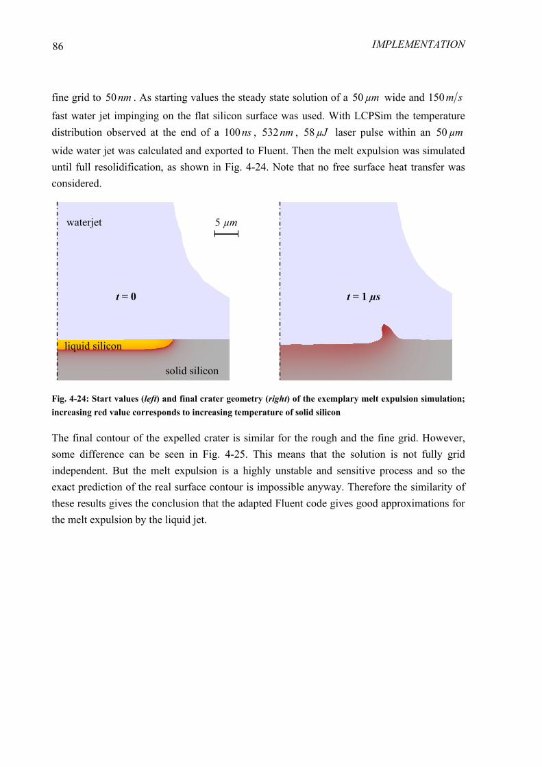
IMPLEMENTATION
86
fine grid to nm50 . As starting values the steady state solution of a µm50 wide and sm150
fast water jet impinging on the flat silicon surface was used. With LCPSim the temperature distribution observed at the end of a ns100 , nm532 , µJ58 laser pulse within an µm50
wide water jet was calculated and exported to Fluent. Then the melt expulsion was simulated until full resolidification, as shown in Fig. 4-24. Note that no free surface heat transfer was considered.
Fig. 4-24: Start values (left) and final crater geometry (right) of the exemplary melt expulsion simulation; increasing red value corresponds to increasing temperature of solid silicon
The final contour of the expelled crater is similar for the rough and the fine grid. However, some difference can be seen in Fig. 4-25. This means that the solution is not fully grid independent. But the melt expulsion is a highly unstable and sensitive process and so the exact prediction of the real surface contour is impossible anyway. Therefore the similarity of these results gives the conclusion that the adapted Fluent code gives good approximations for the melt expulsion by the liquid jet.
waterjet
solid silicon
liquid silicon
t = 0 t = 1 µs
5 µm

IMPLEMENTATION
87
0 5 10 15 20 25 30
−6
−4
−2
0
2
4
6
radial coordinate [µm]
axia
l coo
rdin
ate
[µm
]
100 nm grid50 nm grid
Fig. 4-25: Silicon surface position after 1 µs melt expulsion for different element sizes
Besides evaporation of silicon also evaporation of the liquid jet media is not yet considered within the developed Fluent code. This means that no vapour film at the hot silicon surface is formed. This vapour film is assumed to significantly reduce the visous forces between the liquid jet and the silicon melt. However, the pressure forces exerted by the liquid jet impinginment dominate the visous forces by far. To proof this fact, identical melt expulsion simulations with different viscosities of the liquid jet, smPa8.0 and smPa2.2 , where carried
out, showing no differences of the resulting silicon surface after resolidification. Therefore the decrease of viscous forces due to a vapour layer would not influence the final simulation results and is thus feasible to neglect.
The evaporation of the liquid jet media at the silicon surface additionally changes the pressure forces by recoil pressure and compressibility effects. However, it is assumed that the vapour layer forms smoothly at the beginning of the laser pulse and that it shows a quasi steady state behaviour during the relative long melt duration at constant surface temperature after the laser pulse. This is indicated by the quasi steady state behaviour of the liquid jet temperature during simulations including for surface heat transfer. Furthermore, the thickness of the film should be small in the order of well below one micron, as can be deduced from the sharp temperature drop in Fig. 4-23. So pressure changes are also feasible to negelect as a first approximation.
4.4 Coupling of LCPSim and Fluent
As mentioned before, LCPSim is an efficient simulation program for the thermodynamic and optical effects in laser processing but neglects any fluid dynamical effects. For this Fluent was

IMPLEMENTATION
88
adapted to cope with melt expulsion and by the liquid jet. However, Fluent’s implemented optics models are not suitable for the corresponding optical effects in laser processing. A principal problem is that the simulation of laser light absorption and silicon melting requires a much smaller time step size than the simulation of melt flow, but Fluent is not able to use different time step sizes for different models. For these reasons a transient coupling of LCPSim and Fluent was programmed [61]. This way each physical effect is solved separately and efficiently with suitable time step sizes and grids.
4.4.1 Coupling algorithm
Within the coupled code, LCPSim calculates all effects as usual. However, surface recession due to evaporation is not calculated, i.e. assuming a constant material distribution during each time step. Surface recession corresponds to a movement of the surface and has to be considered within Fluent. Without consideration of a vapour phase, this would mean a mass sink leading to incorrect results for fluid flow. Therefore the coupled code is currently limited to laser pulses which cause no evaporation.
Fluent calculates the fluid flow and heat convection by UDS temperature fields for silicon and water. For the silicon UDS the enthalpy rather than the temperature is used as the scalar, in order to allow a direct exchange of data with LCPSim. Furthermore, interfacial heat transfer can be calculated within Fluent. The heat conduction is calculated by LCPSim rather than by Fluent, because the fast laser heating process has to be resolved by the smaller time step sizes of LCPSim.
Fluent is used as the main program responsible for initialization and controlling of the coupling. It starts by setting the initial values and performing the first time step. Then the data, namely the current time, the current time step size, the silicon distribution silicona and the
silicon enthalpy, is exported to text files via an UDF. Afterwards, Fluent is paused and LCPSim is started. LCPSim reads and interpolates the data and performs time integration over the current Fluent time step size by several smaller time steps. The resulting enthalpy is exported to Fluent and the next time step is calculated by Fluent. Both LCPSim and Fluent watch a file containing an execution flag within an endless loop until the right flag is recognized and each changes the flag after calculation respectively. This workaround is needed, because there is no possibility for external control of Matlab and Fluent during the run. Completely starting and closing Matlab or Fluent during each time step would mean wasting most of the overall computing time. A flow chart explaining the coupling algorithm is given in Fig. 4-26.

IMPLEMENTATION
89
Fig. 4-26: Program flow charts for the coupling algorithm of Fluent and LCPSim; data exchange illustrated by red arrows
The big advantage of the coupled code is the possibility to use different time step sizes and even different grids for optics and thermodynamics on the one hand, and for fluid flow on the other hand. This enables the simultaneous simulation of laser heating and melt expulsion. A disadvantage is that in every time step data exchange and interpolation have to be performed. For typical settings, however, it has been observed that still the dominating part of the computing time is spent for solving rather than data exchange. Keeping in mind the highly customization and adaptation to the problem of the coupled code, this means that the regarding effects are solved very efficiently.
Special care has to taken to the data interpolation between the different grids of Fluent and LCPSim. Here it has to be ensured that the arbitrary silicon surface is always one element sharp. For the enthalpy export to Fluent, the empty elements of LCPSim near the surface are set to the surface enthalpy values. This hinders an interpolation error by Fluent leading to significantly wrong values at the surface. To minimize the error by the multiple interpolations, data exchange is only performed in a predefined region, where liquid silicon could be present. For the regions where only solid silicon is present, no Fluent simulation is necessary, whereas in the region where no silicon is present at all, LCPSim is not applied. The different regions

IMPLEMENTATION
90
are illustrated in Fig. 4-27. In the intersecting region, where the data interpolation occurs, an identical rectangular grid is used both by Fluent and LCPSim.
Fig. 4-27: Illustration of coupled Fluent and LCPSim solution domains with region of identical grid for 2d axial symmetry
4.4.2 Verification
The grid independency of the coupled code is already proven by the grid independency of Fluent and LCPSim. What has to be verificated is the sufficient degree of coupling. To proof this, an exemplary melt expulsion simulation was carried out using different coupling time step sizes. Simulations were performed with Fluent time step sizes of ns2.0 and ns3.0 .
Additionally a data exchange only every two Fluent time steps was applied. In Fig. 4-28 the expelled silicon volume over time is shown. The different curves agree within an error, which is not significant for the interpretation of the results within this work. Also considering the high physical sensitivity of the expulsion process to small changes, this agreement proves the error introduced by the discrete coupling to be small.
LCPSim
data exchange only on identical grid
Fluent
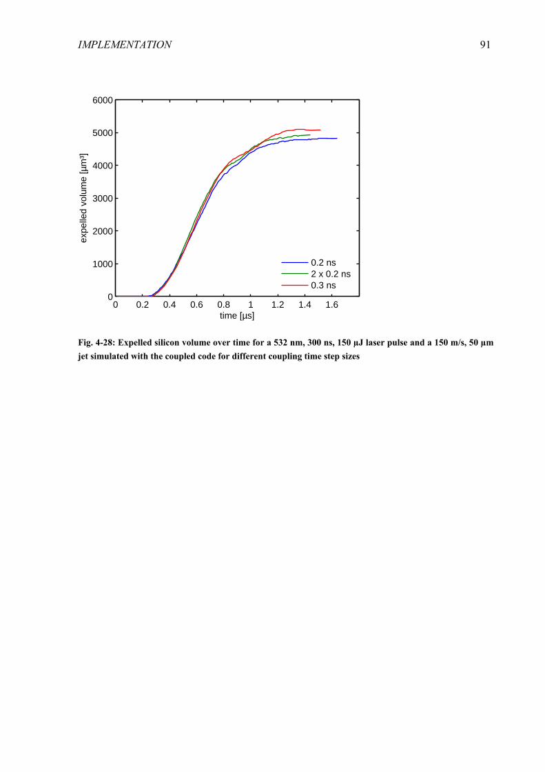
IMPLEMENTATION
91
0 0.2 0.4 0.6 0.8 1 1.2 1.4 1.60
1000
2000
3000
4000
5000
6000
time [µs]
expe
lled
volu
me
[µm
³]
0.2 ns2 x 0.2 ns0.3 ns
Fig. 4-28: Expelled silicon volume over time for a 532 nm, 300 ns, 150 µJ laser pulse and a 150 m/s, 50 µm jet simulated with the coupled code for different coupling time step sizes
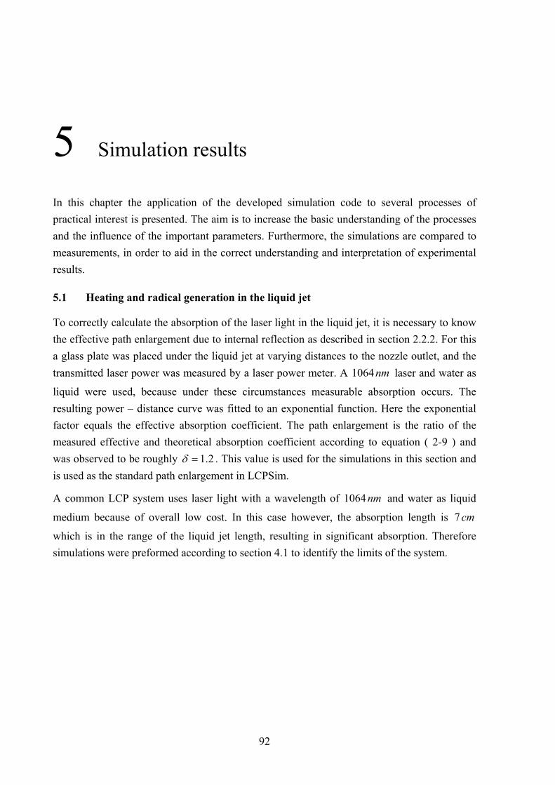
92
5 Simulation results
In this chapter the application of the developed simulation code to several processes of practical interest is presented. The aim is to increase the basic understanding of the processes and the influence of the important parameters. Furthermore, the simulations are compared to measurements, in order to aid in the correct understanding and interpretation of experimental results.
5.1 Heating and radical generation in the liquid jet
To correctly calculate the absorption of the laser light in the liquid jet, it is necessary to know the effective path enlargement due to internal reflection as described in section 2.2.2. For this a glass plate was placed under the liquid jet at varying distances to the nozzle outlet, and the transmitted laser power was measured by a laser power meter. A nm1064 laser and water as
liquid were used, because under these circumstances measurable absorption occurs. The resulting power – distance curve was fitted to an exponential function. Here the exponential factor equals the effective absorption coefficient. The path enlargement is the ratio of the measured effective and theoretical absorption coefficient according to equation ( 2-9 ) and was observed to be roughly 2.1=δ . This value is used for the simulations in this section and is used as the standard path enlargement in LCPSim.
A common LCP system uses laser light with a wavelength of nm1064 and water as liquid
medium because of overall low cost. In this case however, the absorption length is cm7
which is in the range of the liquid jet length, resulting in significant absorption. Therefore simulations were preformed according to section 4.1 to identify the limits of the system.

SIMULATION RESULTS
93
Fig. 5-1: Exemplary intensity loss (left) and heating (right) in the water jet
In Fig. 5-1 the average intensity loss and the temperature distribution over the jet length for pulsed and CW laser power are shown. A water jet produced by a µm50 nozzle with a
velocity of sm150 was used and the applied laser power was W80 with a repetition rate of
kHz13 and a pulse duration of µs1 for the pulsed case. This corresponds to the standard
nm1064 laser used at Fraunhofer ISE for LCP. It can clearly be seen that not only is the
power loss a problem, but also the boiling temperature of water can be reached, which would lead to jet breakup. The temperature peaks induced by the single pulses are equalized over the jet length because of heat conductivity and overlapping of several pulses. Therefore the jet heating by laser pulses is well approximated by considering only the average power and applying the analytical equation ( 4-15 ). This was observed to be true as well for shorter pulse durations down to ns1 .
As a conclusion it is important that for choosing a well suited LCP system, absorption and heating in the liquid jet should be considered. This is especially true for the wafering application, where cuts with high power lasers are performed over several centimetres jet length range, as discussed in [10].
Another effect investigated here is the possibility to generate chlorine radicals by light induced dissociation of chlorine molecules. As mentioned before these radicals are generally much more reactive and should therefore increase the etch rate on silicon. Their presence could improve the speed and quality of etching assisted processes e.g. in the wafering application. One possible approach for this idea is based on coupling a laser into a liquid jet containing chlorine for both silicon heating and radical generation at the same time. The laser wavelength has to be short enough to allow for dissociation of a molecule by the energy of a single photon. This is the case for ultra violet (UV) light, see [63].
0 2 4 6 8 100
0.2
0.4
0.6
0.8
1
jet length [cm]
rela
tive
inte
nsity
0 2 4 6 8 10
20
40
60
80
100
jet length [cm]
tem
pera
ture
[°C
]
pulsed, simulationcw, analytic solution

SIMULATION RESULTS
94
This setup was simulated by the 1d simulation code as described in section 4.1. CW laser light with a wavelength of nm355 and a power of W15 in a liquid jet with a diameter of µm41
and a velocity of sm150 was assumed. As a low reactive and absorptive solvent the
properties of Fluorinert FC770 with 31793 mkg=ρ and KkgJc p 1038= were applied for
the simulations. The inlet molecular chlorine concentration was varied between lmol01.0
and lmol1 .
In Fig. 5-2 the resulting intensity and radical distribution over the jet length are shown. For the highest molecular chlorine concentration the laser intensity drops to zero within the first few millimetres. The radicals generated in this region can not be further transported significantly by the jet flow because of the high radical recombination rate. So for working distances of several centimetres, nearly no laser light or radicals are present. For the low chlorine concentration, the laser light is transmitted significantly to several centimetres, but the generated radical concentration is far too low for practical relevance. There exists no optimum of the molecular chlorine concentration in between where both significant laser power and radical concentration are observed in the several centimetres range. Considering that in current LCP machines the minimum working distance is at least one to two centimetres for technical reasons, the simulation results show that the coupling of an UV laser for radical generation is not applicable. The alternative of a side UV light is also challenging, because the light has to be directed very close to the reaction spot to hinder recombination of the radicals. For the cutting of deep grooves these issues become even more problematic.
Fig. 5-2: Simulated intensity drop and radical concentration for different molecular chlorine concentrations within the liquid
0 0.2 0.4 0.6 0.8 10
0.2
0.4
0.6
0.8
1
jet length [cm]
rela
tive
inte
nsity
0.01 mol/l0.1 mol/l1 mol/l
0 0.2 0.4 0.6 0.8 10
0.5
1
1.5
2
jet length [cm]
radi
cal c
once
ntra
tion
[mm
ol/l]
0.01 mol/l0.1 mol/l1 mol/l

SIMULATION RESULTS
95
5.2 Influence of basic parameters in silicon laser processing
This section aims to gain an understanding of the influence of the basic laser parameters with the restriction to low to medium laser power. As mentioned earlier, for high laser power the models are not sufficiently valid. The parameters of greatest influence in pulsed laser processing are the fluence, the pulse length and the wavelength. There are further parameters like repetition rate, spatial beam profile and pulse shape. But a general influence of these parameters can hardly be obtained because it strongly depends on the individual case. The results of most interest for low to medium power laser processes are the melt depth and the melt duration. Furthermore, the melting and evaporation thresholds are determined so that the relevant parameter regions, for laser doping processes for example, can be identified.
For the parameter study, single pulses have been simulated with the 2d axial symmetric solver of LCPSim. A flat top profile with a relatively large diameter was used, so that lateral effects do not influence the result near the spot centre. Thus the simulation results correspond to a 1d solution.
In Fig. 5-3 and Fig. 5-4 the simulation results for the different wavelengths are shown. The 2d colour plots show the influence of the fluence and the pulse length over several orders of magnitude on the melt duration and melt depth. In addition, the evaporation threshold is indicated, which corresponds to the fluence value where the boiling temperature is overcome. For fluences significantly above the evaporation threshold, the implemented models lose their validity and the results should be taken only as rough approximations. Note that the colour spikes occurred due to converging problems and are not physical.
It has been observed that the wavelengths nm355 and nm532 show nearly the same results
and are therefore not differentiated. This can be explained by the relatively high absorption coefficients for solid silicon in both cases. Thus the non-reflected part of the pulse energy is deposited near to the surface within a distance smaller than the final melting depth. Although the absorption coefficient for nm355 is much higher than for nm532 , see Fig. 2-4, the same
amount of absorbed energy is available for surface melting and evaporation and therefore no significant differences are observed.
The observations using the laser wavelength of nm1064 differ considerably from the
wavelengths nm355 and nm532 . Here the absorption coefficient is relatively low for low
temperatures, which leads to deposition of the pulse energy within a depth much greater than the final melting depth. This energy is not fully available for melting and evaporation at the surface and therefore much higher fluences are needed for the onset of melting. Because the energy is more widely deposited for the wavelength of nm1064 , the resulting temperature

SIMULATION RESULTS
96
gradients after the pulse are lower. This results in lower resolidification speeds, which explains the somewhat higher melt durations and melt depths for equal pulse durations.
Fig. 5-3: Simulated melt durations [µs] for 532 nm (left) and 1064 nm (right) single laser pulses; dashed line corresponds to the evaporation threshold
Fig. 5-4: Simulated melt depths [µm] for 532 nm (left) and 1064 nm (right) single laser pulses
In Fig. 5-5 the melting and evaporation thresholds are plotted against the pulse duration, as they were observed by the single pulse simulations. The thresholds were evaluated also for water with a pressure of bar140 as a typical LCP environment. The melting thresholds are
lowered because the higher refraction index decreases the reflectivity at the silicon surface, see Fig. 2-7. Because of the higher increased surrounding pressure the boiling point is increased according to equation ( 2-34 ), which explains the increased evaporation thresholds.
As explained above, using the wavelength of nm1064 requires more energy to achieve onset
of melting. The melting threshold remains similar for all pulse durations. In contrast to this, the melting threshold for a shorter wavelength is much lower and strongly dependent on pulse duration. The reason for this is the increasing amount of energy conducted away from the
fluence [J/cm²]
puls
e du
ratio
n [µ
s]
5 10 15 2010
−3
10−2
10−1
100
fluence [J/cm²]
puls
e du
ratio
n [µ
s]
25 30 35 4010
−3
10−2
10−1
100
101
100
10−1
fluence [J/cm²]
puls
e du
ratio
n [µ
s]
5 10 15 2010
−3
10−2
10−1
100
fluence [J/cm²]
puls
e du
ratio
n [µ
s]
25 30 35 4010
−3
10−2
10−1
100
0
2 µ
4 µ
6 µ
8 µ
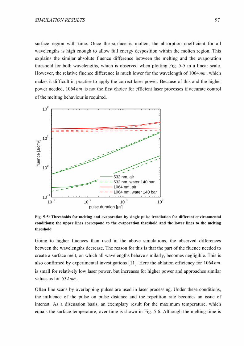
SIMULATION RESULTS
97
surface region with time. Once the surface is molten, the absorption coefficient for all wavelengths is high enough to allow full energy desposition within the molten region. This explains the similar absolute fluence difference between the melting and the evaporation threshold for both wavelengths, which is observed when plotting Fig. 5-5 in a linear scale. However, the relative fluence difference is much lower for the wavelength of nm1064 , which
makes it difficult in practise to apply the correct laser power. Because of this and the higher power needed, nm1064 is not the first choice for efficient laser processes if accurate control
of the melting behaviour is required.
10−3
10−2
10−1
100
10−1
100
101
102
pulse duration [µs]
fluen
ce [J
/cm
²]
532 nm, air532 nm, water 140 bar1064 nm, air1064 nm, water 140 bar
Fig. 5-5: Thresholds for melting and evaporation by single pulse irradiation for different environmental conditions; the upper lines correspond to the evaporation threshold and the lower lines to the melting threshold
Going to higher fluences than used in the above simulations, the observed differences between the wavelengths decrease. The reason for this is that the part of the fluence needed to create a surface melt, on which all wavelengths behave similarly, becomes negligible. This is also confirmed by experimental investigations [11]. Here the ablation efficiency for nm1064
is small for relatively low laser power, but increases for higher power and approaches similar values as for nm532 .
Often line scans by overlapping pulses are used in laser processing. Under these conditions, the influence of the pulse on pulse distance and the repetition rate becomes an issue of interest. As a discussion basis, an exemplary result for the maximum temperature, which equals the surface temperature, over time is shown in Fig. 5-6. Although the melting time is

SIMULATION RESULTS
98
much longer than the pulse duration, the temperature drops nearly to room temperature within a few microseconds. Typical laser pulse frequencies are below kHz100 . This means that the
time between the laser pulses are longer than µs10 , so that for most cases the laser pulses can
be assumed to be thermally independent. This agrees also with experimental results. For example, Rodofili showed that LCP doping line scans produce identical results for pulse frequencies of kHz2 and kHz35 if the pulse overlap and pulse energy are kept constant [64].
0 2 4 6 8 100
500
1000
1500
2000
2500
3000
3500
4000
4500
time [µs]
tem
pera
ture
[K]
0
10
20
30
40
50
60
70
80
90
100
inte
nsity
[MW
/cm
²]
Fig. 5-6: Cooling curve after a 532 nm, 30 ns, 5 J/cm² laser pulse irradiation
Special care in this case has to be taken when using the wavelength of nm1064 . There the
absorption coefficient depends strongly on temperature. That means that the amount of lost pulse energy as discussed above is very sensitive to the initial temperature of the affected silicon volume. In Fig. 5-7 a significant lowering of the melting threshold for higher initial temperatures of the silicon bulk can clearly be seen. Thus, for a nm1064 laser with high
repetition rates, the remaining heat of the previous pulse is able to influence the impact of the following pulse.

SIMULATION RESULTS
99
300 350 400 450 5000
2
4
6
8
10
12
14
16
18
20
22
temperature [K]
fluen
ce [J
/cm
²]
Fig. 5-7: Simulated dependency between melting threshold and initial silicon temperature for a 1064 nm, 30 ns laser pulse
5.3 Dry laser ablation
5.3.1 Silicon
The first quantitative comparisons of simulation and experiment were performed for dry laser scans. A nm1064 laser with a maximum average power of W70 and a pulse length of ns70
was used to cut lines at different scan speeds, average power and repetition rate. After breaking the processed wafer, cross section scanning electron microscope (SEM) pictures were made to measure the groove depth. The Gaussian width of the laser spot could not be determined precisely, and was therefore varied to fit the experimental data, resulting in
µmgauss 30=σ . Simulations were carried out for the same laser parameters using the enthalpy
based evaporation model. Because this is hardly allowed for the applied pulse durations, the resulting transient results have to be taken with care. The high laser power used limits the validity of the results further. However, just by looking at the evaporation depth the simulation should be a feasible approximation, because the energy balance is kept.
Early results were published in [57], where a 2d axial symmetric version model was used for the simulations. This method introduces an error in heat conduction, because the groove geometry is not axially symmetric. However, the heat transport taking place on a spatial scale greater than the groove depth is still well described by the axial symmetric model.

SIMULATION RESULTS
100
3 3.5 4 4.50
10
20
30
40
50
60
70
80
90
100
pulse energy [mJ]
cutti
ng d
epth
[μm
]
60% overlap80% overlap93% overlap
Fig. 5-8: Measured (squares) and simulated (lines) groove depth for different pulse energies and pulse overlaps
Fig. 5-9: Scanning electron microscope (SEM) picture of a groove cross section compared to the simulated groove shape (red line) corresponding to a pulse energy of 4.4 mJ and an pulse overlap of 93 %
Nevertheless the results show good agreement with the experimental data as illustrated in Fig. 5-8 and Fig. 5-9. Also, the evaporated contour is in good agreement with the SEM pictures and follows basically the Gaussian intensity distribution. A lot of particles can be seen lying on the groove surface. They consist of redeposited silicon from the vapour and the liquid phase. This indicates that melt flow and vapour dynamics play a significant role during the ablation process, which is not considered within the simulations. Despite all of these simplifications, the good agreement with the simulation results allows the conclusion, that the

SIMULATION RESULTS
101
dry laser ablation depth quite linearly follows the locally deposited energy, i.e. the fluence. But this can only be stated if pulse energy and pulse length do not differ greatly from the parameters investigated here. From the simulation experience and literature [47] it can be assumed that this linear relation stays true for higher pulse lengths if the process parameters assure staying well above the melting threshold, whereas for shorter pulse lengths vapour dynamics significantly influence the process results.
5.3.2 Silicon nitride layer
A topic of great interest currently in solar cell manufacturing is the local opening of antireflection and passivation coatings by laser ablation. At Fraunhofer ISE a process is investigated where a nm355 laser with pulse lengths around ns130 is used to ablate an anti-
reflection silicon nitride (SiNx) layer. Single pulse experiments were performed by Knorz [65] on a nm280 and nm350 thick SiNx layer on a silicon wafer. The pulse energy was varied
between µJµJ 24.0 − . With a confocal microscope the contour and the depth of the ablation
crater was determined.
For the simulation of the single pulses the 2d axial symmetric multilayer model was used. Most critical was the selection of suitable material properties, because precise data for the required temperature range is not given in current literature. Some temperature dependent data were found in [66] for the heat capacity and the heat conductivity, which were fitted and used as extrapolations up to the boiling point.
[ ]Kkg
JKTc p263.026.59=
[ ]Km
WKTK 3979.032.0=
( 5-1 )
The extinction coefficient was taken from [67] to 21.0=k . The real part of the refraction
index was measured at Fraunhofer ISE as 1.2=n and the density as 3376.2 mkge . Because
SiNx is amorphous, no defined melting point exists, and it can be treated as a liquid at any temperature. Therefore no phase change is considered by setting the latent heat of melting to zero. No data for the boiling point and the latent heat of vaporization has been found in literature. Therefore the average bond energy of SiNx was calculated and assumed to equal the enthalpy needed for full evaporation starting from zero Kelvin. The boiling point was estimated to be K3000 , similar to pure silicon. From these assumptions the enthalpy at the
boiling point was calculated according to equation ( 2-24 ). The latent heat of vaporization is then derived by the difference between the average bond energy and the calculated enthalpy at

SIMULATION RESULTS
102
the boiling point to be 3107.1 mJeLv = . With this calculation, the energy balance is
somewhat independent of the not precisely known boiling temperature. The Gaussian width of the laser spot was derived from experiments to µmgauss 02.2=σ .
In Fig. 5-10 the results are compared, showing good agreement between the simulated and measured curves despite of the rough approximations as discussed above. Note that the parameters were not changed from the original settings to fit the simulation results. This leads to the conclusion that the ablation mechanism is well described by the simulation models. This means that the SiNx is directly thermally ablated, and other mechanisms like lift off or indirect heating play a minor role.
Fig. 5-10: Comparison of simulation and experiment for single pulse ablation of a 350 nm SiNx layer
5.4 Ablation of silicon by LCP
In contrast to dry laser ablation, additional effects have to be considered for ablation by LCP. The impingement of the liquid jet results in increased surrounding pressure at the surface and in melt expulsion. This section shows simulations with LCPSim for ablation by evaporation on the one hand, and with Fluent to account for melt expulsion on the other hand to improve the understanding of the LCP ablation mechanism.
5.4.1 Evaporation
Simulations were carried out with LCPSim to calculate the groove depth for different LCP parameters. As described in section 5.3.1, the 2d axial symmetric solver was used to get approximated results within an acceptable computing time. A flat top profile within the liquid jet diameter is assumed. This is feasible for grooving because of the averaging effect due to the pulse overlap. Furthermore, the increased environmental pressure and refractive index caused by the liquid jet are taken into account. As discussed before, LCPSim does not allow
0 0.5 1 1.50
2
4
6
8
10
12
14
pulse energy [µJ]
crat
er v
olum
e [µ
m³]
simulationexperiment
0 0.5 1 1.50
0.1
0.2
0.3
pulse energy [µJ]
crat
er d
epth
[µm
]
simulationexperiment

SIMULATION RESULTS
103
for the simulation of melt flow. Therefore evaporation is the only considered ablation mechanism for the simulation results shown in this section.
The ablation process was investigated for the high power laser commonly used at Fraunhofer ISE for the wafering application. This laser has a wavelength of nm1064 , a maximum
average power of W80 , a repetition rate of kHz13 and a pulse duration of approximately
µs1 . A parameter study was performed where the nozzle diameter and the scan speed was
varied in such a way that a constant pulse overlap of %75 was achieved. Here the pulse
overlap is defined as the ratio of the liquid jet diameter and the pulse to pulse distance. The resulting groove depths were measured from microscope images of the groove cross section.
0 50 100 150 200 250 300 350 4000
10
20
30
40
50
60
70
80
90
100
fluence [J/cm²]
groo
ve d
epth
[µm
]
experimentsimulation without raytracingsimulation with raytracing
Fig. 5-11: Comparison of measured groove depths with the simulation results; dashed line corresponds to the linear fit of the simulations without consideration of raytracing
In Fig. 5-11 the measured and simulated groove depths are plotted over the laser fluence. With raytracing switched off, i.e. multiple reflections are ignored, the simulated groove depth shows a linear relationship to the laser fluence. This means that using different liquid jet diameters results in the same groove depth if the scan speed and the laser power are chosen in such way that an identical pulse overlap and laser fluence is achieved. For the experimental data no linear relationship can be perceived, but a significant curvature is observed. Furthermore, the measured groove depths for nearly identical fluences vary stronger than could be explained by measurement inaccuracies. This indicates that even at the same laser fluence, the liquid jet diameter has a significant influence on the groove depth. Nevertheless,
SIMULATION RESULTS
104
the ablation threshold agrees very well with the simulations at approximately 240 cmJ as
can be derived from Fig. 5-11.
One possibility to explain the differences of simulated and experimental values is the not considered effect of angular dependent multiple reflection. These effects should be dependent on the groove geometry and therefore on the liquid jet diameter. Therefore the same simulations were carried out using the raytracing feature of LCPSim and the results are also plotted in Fig. 5-11. It can be seen that some scattering is observed, which corresponds to the expected dependency on the liquid jet diameter. A slight curvature is achieved as well.
Although the consideration of raytracing gives qualitatively better agreement of the simulated results with the measurements, the correlation with the experimental results is still low. This means that other physical effects, like melt flow and vapour dynamics, play a significant role. In the low fluence region the liquid jet is assumed to expel the molten silicon, which results in deeper grooves than predicted by evaporation only. For increasing fluences, redeposition of melt and recondensation of silicon vapour takes place and could explain the decreasing slope in Fig. 5-11. Therefore the next step was the investigation of melt flow.
5.4.2 Melt expulsion by the liquid jet
The ablation mechanism of LCP especially for comparably long laser pulse durations is assumed to be dominated by liquid jet driven melt expulsion. Thus, this effect will be investigated here. The first simple model for melt expulsion was implemented in LCPSim by adding an additional constant surface recession speed of sm4.1 if the surface is molten,
derived from a fit to the experimental data. For this the Knudsen evaporation model is used and the additional surface recession speed is added in equation ( 4-54 ). As you can see in Fig. 5-12, this simple model gives already a much better agreement with the experimental results, but is still not satisfactory. This indicates that melt flow induced by the liquid jet plays rather a decisive role and will therefore be investigated in more detail.

SIMULATION RESULTS
105
0 50 100 150 200 250 300 350 4000
10
20
30
40
50
60
70
80
90
100
fluence [J/cm²]
groo
ve d
epth
[µm
]
experimentsimulation with simple melt expulsion model
Fig. 5-12: Measured and simulated groove depths with simple melt expulsion model as described in the text; LCP parameters as described in previous section
Generally, the liquid is not able to accelerate the silicon melt instantaneously due to momentum forces, meaning that it takes some time until significant melt expulsion occurs. To understand the dependence of the ablation mechanism on the laser parameters, it is important to know the time scale for melt expulsion. For this, a simple melt expulsion simulation was carried out using Fluent. First, the steady state jet impingement on a flat silicon surface was calculated. Next, an exemplary melting volume with a depth of µm10 at the silicon surface
was instantaneously set to a liquid phase having the properties of silicon melt. With this state the transient simulation was started as shown in Fig. 5-13. No heat transport is considered and therefore no resolidification of the melt occurs. However, by just looking at the start of the melt expulsion, where no significant solidification takes place, this simplification is feasible.

SIMULATION RESULTS
106
Fig. 5-13: Expulsion of a typical molten volume by the liquid jet without consideration of heat transport and resolidification
The expelled melt volume was plotted against time and was observed to follow an exponential increase as can be seen in Fig. 5-14. The exponential factor represents the characteristic time for significant melt expulsion and is evaluated by an exponential fit. The simulation was performed for a nozzle size of µm100 and for different jet velocities. In Fig. 5-15 the
resulting characteristic time is plotted versus the jet velocity, corresponding well to a reciprocal relationship. This means that the speed of melt expulsion pretty much linearly scales with the jet velocity rather than with jet pressure. If it is necessary to hinder melt flow by the liquid jet, the melting time caused by one laser pulse should be significantly lower than the characteristic expulsion time.
0 0.2 0.4 0.6 0.8 1 1.20
0.1
0.2
0.3
0.4
0.5
time [µs]
expe
lled
volu
me
frac
tion
simulation result−0.0258+0.0229*exp(t/0.3411)
Fig. 5-14: Ratio of expelled volume to initial liquid volume over time for a liquid jet velocity of 100 m/s
water jet
liquid silicon
t = 0 t = 1.5 µs
15 µm

SIMULATION RESULTS
107
0 50 100 150 200 250 3000
0.05
0.1
0.15
0.2
0.25
0.3
0.35
0.4
0.45
jet velocity [m/s]
char
acte
ristic
exp
ulsi
on ti
me
[µs]
simulationinversely proportional fit
Fig. 5-15: Characteristic time for silicon melt expulsion derived from an exponential fit to the simulated expelled volume over time
To further understand the ablation by melt expulsion, simulations with consideration of laser light absorption and resolidification were performed. Here the coupled code as described in section 4.4 was applied to two different single laser pulses that can be generated in the LCP systems available in laboratory. The first pulse has a wavelength of nm532 and a pulse
duration of ns15 and is called “short pulse” in the following. The second pulse, called “long
pulse”, has a pulse duration of µs3.1 and a wavelength of nm1064 . Because the coupled
code is not able to consider evaporation, the pulse energy was chosen just below the evaporation threshold. The same water jet properties with a velocity of sm140 and a
diameter of µm83 , corresponding to a nozzle diameter of µm100 , were used in both cases. A
flat top intensity profile within the liquid jet was assumed.
Fig. 5-16: Melt expulsion dynamics for the long pulse setup simulated with the coupled code; increasing red value corresponds to increasing temperature of solid silicon
t = 1.2 µs t = 2.1 µs t = 3.6 µs
15 µm

SIMULATION RESULTS
108
In Fig. 5-16 simulation results at different points in time for the long pulse are shown. The cooling of the silicon melt due to heat conduction leads to resoldification around the edges of the reaction spot. Moreover, some droplets detaching from the silicon melt and taken away by the liquid jet can be seen, which corresponds to the silicon particles in the waste water observed in experiment. Full resolidification is reached after µs3.5 , which is significant
lower than the melt duration of above µs10 as predicted without considering melt flow, see
Fig. 5-3. The reason for this is that heat is spread over a large volume by the melt flow, thus increasing the overall cooling speed. This means that the melt durations and melt depths shown in Fig. 5-3 and Fig. 5-4 are overestimated for the case of LCP using pulses which cause a melt duration above the characteristic expulsion time of Fig. 5-15.
The final contour in the simulation after resolidification for both laser pulses is shown in Fig. 5-17. Because of the smaller melt duration for the short pulse, only little movement of the melt takes place and results in a hump looking like a small wave with a size of a few micrometers. The long pulse induces much more melt expulsion and ends up in a hump with a lateral size on the order of µm10 . These hump sizes are in good agreement with the
experimentally observed melt flow structures shown in Fig. 5-18. Here LCP lines with overlapping pulses corresponding to the simulated pulses were processed. The reason for the virtually smaller laser spot size of about one third of the liquid jet diameter is the inhomogeneous intensity profile within the jet. It shows somewhat higher intensities near the centre and decreasing intensities to the edges. The inhomogeneities in the intensity profile are also the reason for the randomly located melt waves observed for the short pulse, rather than having one ring as in the simulation result.
Fig. 5-17: 3d view of simulated silicon surface after full resolidification for the long pulse (left) and the short pulse (right) setup

SIMULATION RESULTS
109
Fig. 5-18: Scanning electron microscope (SEM) pictures of LCP processed silicon surfaces by overlapping laser pulses corresponding to the long pulse (left) and the short pulse (right) setup; note the different scales
In conclusion, the size of the experimental melt flow structures can be explained by the melt expulsion simulations. For nanosecond laser pulses the melt flow induced by the liquid jet is only small. This is assumed to introduce minor crystal damage and is therefore suitable for LCP applications where a good quality has to be achieved, e.g. the doping processes. The longer the pulse durations, which result in longer melt durations, the higher is the amount of melt expulsion. For a pulse duration of around µs1 , significant melt movement was observed
in the simulations and is identified as the main ablation mechanism for low pulse energies. This agrees with the relatively large experimental groove depths for low fluences in Fig. 5-11 and Fig. 5-12. Because melting and melt removal requires less energy than evaporation, the melt expulsion ablation mechanism is more efficient and therefore suitable for wafering applications.
5.4.3 Cooling effect
It is often mentioned that a big advantage of the liquid jet guided laser is the high insitu cooling effect, which reduces the thermal impact and therefore produces clean cuts with low damage in the processed material [7, 68]. Especially for silicon solar cell manufacturing crystal damage caused by thermal stress is a very important issue in laser processing as it can seriously decrease the solar cell efficiency. Therefore it is worthwhile to have a closer look at the cooling effect in LCP.
A high indirect cooling effect takes place if the ablation mechanism is dominated by melt removal. Here the heat is removed together with the melt and is this way transported away from the reaction zone. This is an advantage to dry laser processing, where a high fraction of the expelled and evaporated silicon is redeposited around the reaction spot. Thus for long pulse duration or CW, LCP is assumed to introduce less, but still significant, remaining heat and thermal stress.
SIMULATION RESULTS
110
Another cooling mechanism is radiation from the silicon melt surface. This effect is included into the simulations according to equation ( 2-26 ) and was observed to be not relevant at all.
The second direct cooling mechanism is the heat transfer to the liquid jet at the melt surface. The high speed impinging jet shows a very high heat transfer coefficient around
)(10 26 KmW , as derived from the Fluent simulations, see for example Fig. 4-22. Besides,
the heat conduction into the silicon bulk is also quite fast because of the high heat conductivity of silicon. Typically the temperature below the surface changes about K1000
over a spatial scale of a few micrometers. This results in a corresponding heat transfer
coefficient for heat conduction into the silicon bulk of around )(10 27 KmW , which is
somewhat larger than the surface heat transfer coefficient, but can be on the same order of magnitude. To estimate the influence of this direct cooling effect, melt expulsion simulations were carried out with consideration of surface heat transfer as described in section 4.3.3. The same parameters as for the “long pulse” of the previous section were applied. Only the pulse energy was slightly increased to have comparable values for the final melt duration and melt depth. This was achieved by increasing the pulse energy by approximately %9 . This small
increase shows that only a small amount of the totally absorbed heat is transferred to the liquid jet. Evaporation of the liquid was not considered in the simulations. Because the liquid is in contact with the silicon at melt temperature, a small vapour film is supposed to be formed in real world conditions, acting as a thermal insulation layer. Therefore the cooling effect is even smaller than predicted by the simulations.
Nevertheless cooling takes place and influences the melt expulsion behaviour. In Fig. 5-19 the simulation results for the long pulse including free surface heat transfer is shown. The main difference to the previously shown simulation is that no smooth solid hump forms at the edge of the reaction spot. Because of the cooling of the melt, resolidification takes place before reattaching to the silicon surface. This results in several overlapping layers of resolidified silicon. These layers correspond to the melt flow structures observed in experiments, as shown in detail in Fig. 5-20.
For significantly shorter laser pulses without notable melt expulsion, the direct cooling effect is even smaller because of shorter cooling time and is therefore negligible.

SIMULATION RESULTS
111
Fig. 5-19: Melt expulsion dynamics for the long pulse with consideration of free surface heat transfer
Fig. 5-20: SEM picture of the flow structure detail corresponding to the left image of Fig. 5-18
5.5 Dry laser doping
A promising process under development at Fraunhofer ISE is local doping by dry laser processing [69]. Here the phosphorous silicate glass (PSG) remaining after the high temperature emitter diffusion process acts as a finite dopant source. The laser locally melts the silicon surface und the phosphorous diffuses out of the PSG into the melt. The laser intensities must not be too high to hinder evaporation of the dopant source layer. Because the laser intensities are only slightly above the melting threshold and no melt movement by external forces takes place, dry laser doping is supposed to be well approximated by the models implemented in LCPSim.
Experiments and simulations with LCPSim for dry laser doping were performed by Wühterich [70]. A nm355 laser with a pulse energy of µJ8.3 and a pulse duration of ns40
was used to process line scans with different scan speeds. The Gaussian width of the laser profile in the focal plane was hard to determine precisely in the experiment and was therefore used as a fit parameter for the simulations. In LCPSim the finite source boundary condition is most appropriate to the doping process out of the PSG. Here the initial loading could also not be measured and was used as a second fit parameter. Note that the same values for the fit parameters were used for all simulations.
t = 1.2 µs t = 2.64 µs t = 3.6 µs
15 µm
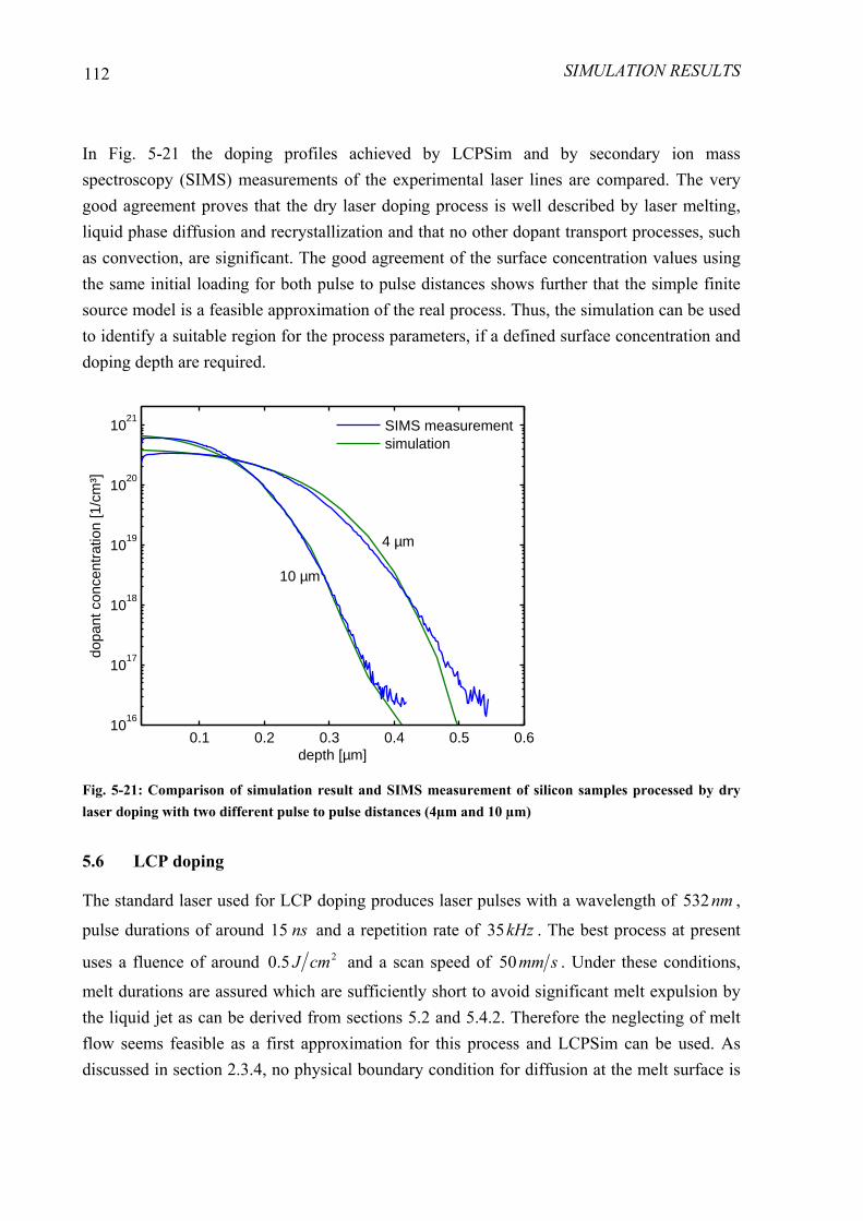
SIMULATION RESULTS
112
In Fig. 5-21 the doping profiles achieved by LCPSim and by secondary ion mass spectroscopy (SIMS) measurements of the experimental laser lines are compared. The very good agreement proves that the dry laser doping process is well described by laser melting, liquid phase diffusion and recrystallization and that no other dopant transport processes, such as convection, are significant. The good agreement of the surface concentration values using the same initial loading for both pulse to pulse distances shows further that the simple finite source model is a feasible approximation of the real process. Thus, the simulation can be used to identify a suitable region for the process parameters, if a defined surface concentration and doping depth are required.
0.1 0.2 0.3 0.4 0.5 0.610
16
1017
1018
1019
1020
1021
depth [µm]
dopa
nt c
once
ntra
tion
[1/c
m³]
SIMS measurementsimulation
4 µm
10 µm
Fig. 5-21: Comparison of simulation result and SIMS measurement of silicon samples processed by dry laser doping with two different pulse to pulse distances (4µm and 10 µm)
5.6 LCP doping
The standard laser used for LCP doping produces laser pulses with a wavelength of nm532 ,
pulse durations of around ns15 and a repetition rate of kHz35 . The best process at present
uses a fluence of around 25.0 cmJ and a scan speed of smm50 . Under these conditions,
melt durations are assured which are sufficiently short to avoid significant melt expulsion by the liquid jet as can be derived from sections 5.2 and 5.4.2. Therefore the neglecting of melt flow seems feasible as a first approximation for this process and LCPSim can be used. As discussed in section 2.3.4, no physical boundary condition for diffusion at the melt surface is

SIMULATION RESULTS
113
applied. Therefore the surface concentration surf
C within the infinite source boundary
condition is set to the surface concentration of the corresponding measured doping profiles.
5.6.1 Simulations with flat top profile
Due to the spatial averaging of the inhomogeneous intensity profile by the high pulse overlap applied in the standard doping process, it is feasible to use a flat top intensity profile as a first approximation. To simulate several overlapping pulses within practicable computing times, the 2d axial symmetric version of LCPSim was used. This is correct for the heat transfer with shallow grooves, as discussed in section 5.3.1. The dopant distribution after several pulses is not axially symmetric. However, most of the diffusion takes place in z -direction and the lateral diffusion affected by the axial symmetric formulation plays only a minor role, especially for the flat top case. Thus, the results for temperature and dopant distribution are well approximated by the axial symmetric model. To consider evaporation, the Knudsen model was chosen due to the relatively short pulse duration.
In Fig. 5-22 two different doping profiles of LCP lines achieved by SIMS measurements are shown as dopant concentration values over the depth from the surface. One SIMS profile corresponds to the best LCP solar cell processed so far with %4.20 efficiency [13]. The
doping profile produced with the same laser parameters, but a higher fluence is also given. Furthermore, the simulation result for the %4.20 parameters is plotted. Both the simulated
and the measured profile for the %4.20 parameters show a similar smooth decrease of dopant
concentration within µm1 to µm5.1 . This indicates that the dopant transport process is well
described by laser melting and liquid phase diffusion as implemented in LCPSim. The differences between the simulated and the measured profile are due to the inhomogeneous intensity profile within the liquid jet, as discussed in detail in section 5.6.2. For the higher pulse energy, a different shape of the doping profile is achieved. The doping depth is increased and a strongly varying curvature is observed, which is not achievable by simulations with LCPSim. This means that for the higher pulse energy, other transport processes besides liquid phase diffusion must play a significant role. For LCP doping experiments with higher pulse duration, similar non smooth doping profiles were measured. Here it is obvious that due to significant melt flow induced by the liquid jet, convectional transport of the dopant takes place. This is assumed to be the reason for the different curve shape in comparison to the pure liquid phase diffusion process. For the shorter pulse durations but higher pulse energies, it is assumed that melt flow induced by evaporation and recoil pressure leads to convectional transport processes.

SIMULATION RESULTS
114
0 0.5 1 1.510
16
1017
1018
1019
1020
1021
depth [µm]
phos
phor
ous
conc
entr
atio
n [1
/cm
³]
simulation, 20.4 % solar cellSIMS, 20.4 % solar cellSIMS, high pulse energy
Fig. 5-22: Doping profiles after LCP doping derived from SIMS measurements and simulation results
The interpretation of the dopant transport mechanisms can be applied to the measured solar cell efficiencies. For the LCP doping parameters using high pulse energies or high pulse durations, no reasonable solar cell efficiencies have yet been achieved at Fraunhofer ISE. Recombination in the space charge region was identified as the primary reason for this, see [14]. Furthermore, Rodofili showed that for the high fluences a great fraction of the phosphorous is electrically inactive [64]. This leads to the conclusion that melt movement and convectional dopant transport reduces the overall doping quality with respect to solar cell efficiency. Considering the small pulse to pulse distance of µm4.1 for the standard scan
speed of smm50 , the final line consists only of the outer regions of a single pulse impact as
illustrated in Fig. 5-23. The outer regions are much more affected by melt flow than the inner region and are therefore assumed to show a worse doping quality. Using lower pulse overlaps, the inner region of a single pulse impact becomes more dominant and should in this way significantly increase the overall doping quality. Unpublished experiments at Fraunhofer ISE showed an improvement of the electrical characteristics of LCP processed silicon samples using higher pulse energies with lower pulse overlap and confirm this theory.

SIMULATION RESULTS
115
Fig. 5-23: Illustration of the influence of the pulse overlap on the surface quality
5.6.2 Influence of inhomogeneous intensity profile
Some experimental observations using low pulse energies could not be described by the simulations with the flat top intensity profile. For example, microscope pictures of LCP processed silicon samples show structures with a size much smaller than the liquid jet diameter, see Fig. 5-24. Furthermore, in experiments an LCP doping effect is observed even for average fluences significantly below the melting threshold. For example in [64] a change
in electrical properties starts at around 21.0 cmJ , although simulations predict a melting
threshold of 235.0 cmJ for the corresponding pulse duration. The reason for this was
assumed to be the inhomogeneous intensity profile within the liquid jet cross section and was therefore investigated in more detail.
Fig. 5-24: Microscope images of LCP processed silicon samples using the standard doping parameters with low fluences; left: 9 single pulses; right: four lines produced by high pulse overlap
First, measurements of the intensity profile were carried out. For this aim a glass plate was placed in such a way that the liquid jet impinges normally onto it. The plate was imaged onto a CCD camera using a microscope objective. Very low laser intensities had to be used to
high overlap low overlap
„good“ doping quality „bad“ doping quality
50 µm 50 µm
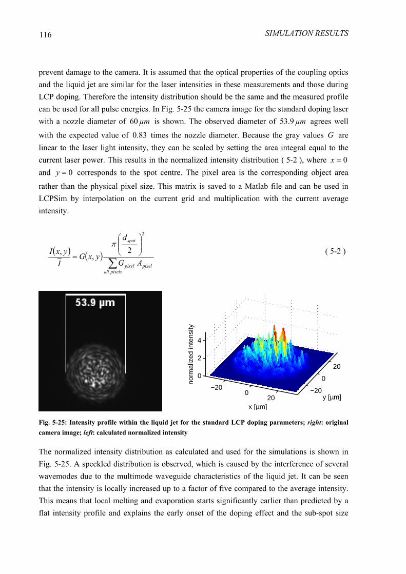
SIMULATION RESULTS
116
prevent damage to the camera. It is assumed that the optical properties of the coupling optics and the liquid jet are similar for the laser intensities in these measurements and those during LCP doping. Therefore the intensity distribution should be the same and the measured profile can be used for all pulse energies. In Fig. 5-25 the camera image for the standard doping laser with a nozzle diameter of µm60 is shown. The observed diameter of µm9.53 agrees well
with the expected value of 83.0 times the nozzle diameter. Because the gray values G are linear to the laser light intensity, they can be scaled by setting the area integral equal to the current laser power. This results in the normalized intensity distribution ( 5-2 ), where 0=x and 0=y corresponds to the spot centre. The pixel area is the corresponding object area
rather than the physical pixel size. This matrix is saved to a Matlab file and can be used in LCPSim by interpolation on the current grid and multiplication with the current average intensity.
( ) ( )∑
⎟⎟⎠
⎞⎜⎜⎝
⎛
=
pixelsallpixelpixel
spot
AG
d
yxGI
yxI
2
2,,
π ( 5-2 )
Fig. 5-25: Intensity profile within the liquid jet for the standard LCP doping parameters; right: original camera image; left: calculated normalized intensity
The normalized intensity distribution as calculated and used for the simulations is shown in Fig. 5-25. A speckled distribution is observed, which is caused by the interference of several wavemodes due to the multimode waveguide characteristics of the liquid jet. It can be seen that the intensity is locally increased up to a factor of five compared to the average intensity. This means that local melting and evaporation starts significantly earlier than predicted by a flat intensity profile and explains the early onset of the doping effect and the sub-spot size
−200
20−20
0
200
2
4
norm
aliz
ed in
tens
ity
x [µm]y [µm]

SIMULATION RESULTS
117
structures. Note that this intensity profile was observed to be constant with time and is therefore assumed to be also constant during LCP processing.
Simulations with flat top and the measured intensity profile were used to get quantitative information on the influence of the local intensity peaks. For the case of the real intensity profile, the full 3d version of LCPSim has to be used with a sufficiently small lateral grid size to approximate the profile adequately. This results in computing times for single pulses on the order of hours to days. Therefore mainly single pulses and only few line scans could be simulated.
In Fig. 5-26 the maximum melt depth and evaporation depth are shown as functions of the average laser fluence with the standard LCP doping parameters applied. The pulse duration varies between ns13 and ns20 , depending on the pulse energy, and was set to experimentally
measured values. Note that in the case of the real intensity profile the maximum melt and evaporation depth is only reached locally at the intensity peaks. It can be seen that the curve with the real profile is roughly shifted to fluence values of a fifth of the flat top ones. This is explained by the local intensity superelevation of a factor of five. Furthermore, the saturation melt depth is only slightly lower than in the flat top case. This means that lateral heat transfer does not significantly reduce the impact of the intensity peaks.
Next, LCP line scans with smm50 scan speed and real intensity profile were simulated with
a more rough grid in the z -direction than for the single pulses. This reduces the computing time significantly but does not sufficiently resolve the molten layer. Therefore no melt depth data for low fluences is plotted in Fig. 5-26. However, the melt depth is close to the value of the corresponding single pulse. Comparison of the results with the fluence threshold of
225.1 cmJ shown in Fig. 1-5 indicates that the emitter quality drops rapidly if the
evaporation depth approaches the range of the initial emitter doping, which was in this case roughly µm5.1 . This could be explained by crystal damage introduced into the space charge
region. For low fluences, the crystal damage is located above the space charge region, and is therefore efficiently shielded.
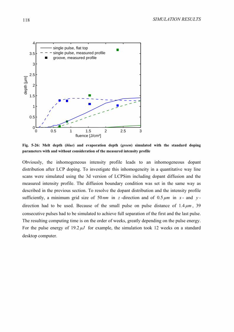
SIMULATION RESULTS
118
0 0.5 1 1.5 2 2.5 30
0.5
1
1.5
2
2.5
3
3.5
4
fluence [J/cm²]
dept
h [µ
m]
single pulse, flat topsingle pulse, measured profilegroove, measured profile
Fig. 5-26: Melt depth (blue) and evaporation depth (green) simulated with the standard doping parameters with and without consideration of the measured intensity profile
Obviously, the inhomogeneous intensity profile leads to an inhomogeneous dopant distribution after LCP doping. To investigate this inhomogeneity in a quantitative way line scans were simulated using the 3d version of LCPSim including dopant diffusion and the measured intensity profile. The diffusion boundary condition was set in the same way as described in the previous section. To resolve the dopant distribution and the intensity profile sufficiently, a minimum grid size of nm50 in z -direction and of µm5.0 in x - and y -
direction had to be used. Because of the small pulse on pulse distance of µm4.1 , 39
consecutive pulses had to be simulated to achieve full separation of the first and the last pulse. The resulting computing time is on the order of weeks, greatly depending on the pulse energy. For the pulse energy of µJ2.19 for example, the simulation took 12 weeks on a standard
desktop computer.

SIMULATION RESULTS
119
Fig. 5-27: Simulated phosphorous surface concentration [log10(cm-3)] for the standard LCP doping parameters with a pulse energy of 8.4 µJ; left: after first pulse; right: after 15 pulses
In Fig. 5-27 the surface dopant concentration after the first and after 15 pulses for relatively low pulse energy is shown. After the first pulse the dopant distribution follows the intensity distribution. Because of the low pulse energy, the threshold fluence for melting is reached only at the intensity peaks and widely non-doped areas exist. After multiple pulses the doping distribution is well homogenized, i.e. a continuous doped line with a width of about µm40 is
achieved. For higher pulse energies even a higher degree of homogeneity is observed as the melting threshold is reached in a greater area.
Fig. 5-28: Simulated phosphorous concentration [log10(cm-3)] in a cross section at x = 125 µm after 15 pulses with a pulse energy of 30 µJ
80 100 120 140 160
60
80
100
120
140
x [µm]
y [µ
m]
16
17
18
19
20
21
80 100 120 140 160
60
80
100
120
140
x [µm]
y [µ
m]
70 80 90 100 110 120 130
0
5
10
15
y [µm]
z [µ
m]
16
17
18
19
20
21

SIMULATION RESULTS
120
70 80 90 100 110 120 1300
0.2
0.4
0.6
0.8
1
1.2
1.4
1.6
1.8
2
y [µm]
z [µ
m]
groove depthdoping depth
Fig. 5-29: Simulated groove depth and doping depth underneath the surface for the same cross section as in Fig. 5-28; doping depth corresponds to the distance between the groove surface and the 1e16 cm-3 isosurface of the dopant concentration
In Fig. 5-28 the cross section of a LCP groove is shown in the real aspect ratio. A pulse
energy of µJ30 was used, which corresponds to an average fluence of 254.1 cmJ and a bad
solar cell efficiency in experiment, see Fig. 1-5. Because of the high simulation time, only 15 pulses could be simulated. This means that the first and the last pulse are still overlapping and therefore the cross section is not fully developed. But it can be used as a first approximation, and basic conclusions can already be derived. Furthermore, it has been observed that the results are only weakly dependent on the x -position of the cross section. This is due to the low pulse on pulse distance of µm4.1 .
The dopant distribution shows a significant doping everywhere underneath the groove
surface. In Fig. 5-29 the doping depth is plotted, which is defined by the 3161 −cme isosurface
of the concentration. The doping depth varies between µm6.0 and µm5.1 underneath the
groove and is more flat directly underneath the groove peaks. Note that outside of the groove an additional doping exists by the initial emitter, which is not shown in the Figure. The final doping distribution is sufficient to prevent shunting of the silicon bulk with the surface metallization. This leads to the conclusion that the inhomogeneity of the dopant distribution should not be a major problem for the resulting doping quality and can not explain the bad solar cell efficiency. It is rather assumed that the intensity peaks locally introduce crystal damage, for example by recoil pressure induced melt flow. For this pulse energy the damage

SIMULATION RESULTS
121
depth reaches deeper than the created doping depth. This leads to recombination in the space charge region, as mentioned before.
For the pulse energy of µJ2.19 , the SIMS measurement of the corresponding experiment is
compared with the simulated doping profile. For the experimental SIMS measurement and the doping profile calculation as described in section 4.2.7, an ion beam with µm10 diameter was
used. The good agreement shown in Fig. 5-30 proves that the LCP doping process is very well described by LCPSim with consideration of the measured intensity profile. Note that the only adjusted parameter was the dopant surface concentration and all other parameters were used as originally implemented. The remaining differences can be explained primary by the use of an exemplary intensity profile in the simulations, which is different from the actual profile during the experiment. Also slight melt flow could have influenced the measured doping profile.
0 0.5 1 1.510
16
1017
1018
1019
1020
1021
depth [µm]
dopa
nt c
once
ntra
tion
[1/c
m³]
simulationSIMS measurement
Fig. 5-30: Simulated and measured doping profile for the standard LCP doping parameters with a pulse energy of 19.2 µJ and consideration of real intensity profile
122
6 Summary
The aim of this work was to develop multiphysics simulation capabilities to describe the effects in LCP for silicon processing and gain in this way an understanding of the general process underlying them. The high degree of coupling of optics, thermodynamics and fluid dynamics exceeds the capabilities of available commercial simulation tools. Therefore great effort had to be undertaken to implement individual solutions on the one hand and extend commercial software, namely Fluent, on the other hand for solving the corresponding mathematical models.
The investigation started with phenomena taking place in the liquid jet before impinging on the silicon surface. Here the physics are not that complex and could be described by analytical equations and a simple finite differences code. By the calculations it has been observed that using a significantly absorbing liquid media, for example water at a laser wavelength of
nm1064 , does not only result in high laser power loss, but can also heat up the jet to critical
temperatures. This has to be considered especially for the wafering application, where the working distance varies in the range of several centimetres.
To enhance the etching of silicon during LCP by generating chlorine radicals within the jet, which are much more reactive, an idea was to couple a laser with a sufficiently short wavelength into a liquid jet to decompose dissolved molecular chlorine. Simulations were carried out by applying a nm355 laser and a nonreactive and non-absorbing solvent
containing different molecular chlorine concentrations. In no case was it possible to have a significant radical concentration at a practical working distance, mainly because of the high recombination rate. Therefore this idea was shown to be not applicable.
The main effort within this work was done to develop LCPSim, a finite differences code programmed in Matlab. LCPSim is able to simulate optical effects like laser light absorption and reflection, and thermodynamic effects, namely heat transport, phase changes, evaporation and dopant diffusion. An algorithm for adaption of a non equidistant grid in every time step was implemented as well as the alternating direction explicit (ADE) time integration method. Furthermore, a semi-analytic treatment of the surface elements and an additional grid coarsening within the time between the laser pulses was introduced. All these techniques result in a very efficient and therefore fast simulation code, which enables even full 3d
SUMMARY
123
simulations of several overlapping pulses, as it occurs in most laser processes for solar cell manufacturing.
The main simplification of LCPSim is the neglecting of fluid dynamics and a vapour phase. So no melt flow and interaction with silicon vapour, as for example recondensation or recoil pressure, can be considered. Furthermore, the evaporation of the liquid jet media and its impact to the melt expulsion dynamics are neglected. However, this was discussed to be a feasible approximation. The development of a self programmed Navier Stokes solver including a suitable multiphase model would have been far too much effort within the frame of this work, so the powerful commercial software Fluent was chosen for simulation of fluid dynamics. Fluent also provides additional models for heat transport and optics, but these were observed to show some limitations for the case of LCP. These limitations have been overcome by using the C-interface of Fluent for customization and implementation of additional models. Separate temperature fields have been implemented to hinder numerical heat diffusion at the free surface between the silicon melt and the liquid media. Furthermore, a transient coupling with LCPSim was developed, which enables the fully coupled simulation of optics, thermodynamics and fluid dynamics in an efficient and numerically stable way. The major restriction of this coupled code is that evaporation can not be considered without an additional vapour phase, which was not yet implemented up to the end of this work.
The simulation capabilities were then applied to practical processes, as they are under development for the manufacturing of silicon solar cells. First of all, a general parameter study was performed to show the influence of the basic laser parameters, namely fluence, pulse duration and wavelength, on the melting and evaporation behaviour. It has been observed that when using a wavelength of nm1064 with moderate fluences, the results are
very sensitive to parameter changes and a practical process is therefore more critical to control than for example with a wavelength of nm532 .
To gain an understanding of different ablation mechanisms, simulation results were compared with experimental data for grooving of silicon by pulsed laser line scans. For dry laser processing an approximately linear relationship between laser fluence and groove depth has been observed, which is in reasonable agreement with the simulation using the enthalpy based evaporation model. Even for silicon nitride, for which it was not possible to determine exact material properties, a good agreement of the ablation threshold and the crater depths has been achieved. This means that in the investigated parameter region, the amount of ablated material follows quite linearly the induced energy.
This linear relation has not been observed for ablation by LCP using laser pulses with a pulse duration of around µs1 , which is currently favoured for the wafering application. Here, the
experimentally observed groove depths are underpredicted by simulations with LCPSim at
SUMMARY
124
low fluences, and overpredicted at high fluences. One major reason for these differences was identified to be melt flow induced by the liquid jet. Multiphase fluid flow simulations were used to calculate a characteristic expulsion time, which is the time scale on which expulsion dynamics takes place. If melt durations are lower than this characteristic time, no significant melt flow induced by the liquid jet takes place. For a more detailed investigation of the expulsion dynamics, the coupled code was used to simulate the final crater contour after resolidification for two different typical LCP laser pulses. The size of the melt flow structures agree well with the experimentally observed ones. Furthermore, a simulation including free surface heat transfer has shown even better agreement of the melt flow structures, although the total heat transferred to the liquid jet is much smaller than the heat conducted into the silicon bulk.
Because laser doping for the manufacturing of selective emitters is currently under intensive research, LCPSim was applied to the different doping processes investigated at Fraunhofer ISE. For the dry laser doping, where a phosphorous containing layer on the silicon surface is used as the dopant source, a very good agreement of the experimentally measured and simulated doping profile has been achieved. This proves that this process is well described by liquid phase diffusion as it is implemented in LCPSim and that no other transport processes for phosphorous play a significant role.
The most promising LCP application is a single step doping by using a phosphorous containing liquid, typically phosphoric acid. The simulations were applied to LCP doping to understand the process and give explanations for the observed results. For the current best process parameters, where a nm532 , ns15 pulsed laser with pulse energies just above the
melting threshold is used, melt flow has been observed to play a minor role. Therefore good agreement of the shape of the doping profile can be achieved by LCPSim. For higher pulse energies and higher pulse durations, the measured doping profiles are very different from the simulated ones. Convective dopant transport by melt flow is proposed to be the reason for the differently shaped doping profiles.
For LCP doping the inhomogeneous intensity profile in the liquid jet cross section was assumed to have great influence on the doping process and was therefore investigated in detail. First, the intensity profile for the standard doping parameters was measured. The normalized profile showed peaks up to a factor of five above the average intensity. This intensity distribution was imported into LCPSim and 3d simulations at different fluences were carried out. The results show much earlier local onset of melting and evaporation than for the flat top case, which explains the experimentally observed early onset of an LCP doping effect. Furthermore, the simulated fluence threshold, where the groove depth reaches the initial emitter depth, correlates with the threshold of solar cell efficiency. So the crystal damage,

SUMMARY
125
which is thermally introduced underneath the emitter depth and therefore also in the space charge region, could be an explanation for the efficiency drop.
For one good quality standard doping process, a 3d simulation considering the real intensity profile and a full line scan was carried out. This 12 week simulation would have been impossible without the efficient programming of LCPSim. The resulting doping profile shows excellent agreement with the measured one. Considering that the surface dopant concentration was the only fit parameter, the standard LCP doping process is very well described by LCPSim and can be simulated without major simplifications.
The main conclusions for LCP doping are listed in the following points:
• For the standard parameters, the single pulse does the doping. The pulses are thermally independent from each other up to several hundreds of kilohertz repetition rate.
• For the standard pulse durations, the melt time is short enough to hinder significant melt flow induced by the liquid jet. Furthermore, evaporation and therefore melt flow induced by the recoil pressure is not significant for the standard pulse energy.
• Melt flow caused by higher pulse energy or higher pulse duration than for the standard doping parameters seems to introduce a bad quality doping. This could be due to crystal damage and inactive phosphorous.
• The intensity profile created by the multimode waterjet shows peaks with intensity values up to five times above the average intensity. This has great impact on the thresholds of melting and evaporation, as well as on the spatial melt and dopant distribution.
• The LCP doping process with the standard parameters is very well described by LCPSim considering the measured intensity profile. This means that aside from liquid phase diffusion no other transport mechanisms contribute significantly to the final dopant distribution.
• The pulse overlap equals out the final doping inhomogeneities, so no poorly or very flat doped regions within the processed line width exist.
• Thermally induced crystal damage is assumed to reach the space charge region when the evaporation depth locally comes in the range of the initial emitter depth. This could be a reason for the experimentally observed drop of solar cell efficiency.
• The parameter window for achieving good quality doping should be enhanced, if the inhomogeneities in the intensity profile are reduced.

SUMMARY
126
To further improve the simulation capabilities, the next important step should be to implement a vapour phase in Fluent and apply an evaporation model at the free melt surface. Because Fluent is able to simulate combined compressible and incompressible multiphase flow and a method to apply transfer mechanisms at the free surface was developed already for the heat transfer, the incorporation of the vapour phase should be in principle possible. Then the effects of recondensation and recoil pressure can be considered additionally. Furthermore, a physical model of the diffusion boundary condition for LCP doping should be developed, because here at present the surface concentration has to be set to an arbitrary value.
In conclusion, basic simulations capabilities for LCP have been successfully developed. They are able to describe and explain a variety of experimentally observed effects and have the potential for further extensions.
127
7 Deutschsprachige Zusammenfassung
Ziel der Arbeit war es, eine Multiphysik Simulationsumgebung zu schaffen um die verschiedenen Effekte beim LCP zur Bearbeitung von Silicium zu beschreiben und auf diesem Wege das Verständnis dieses Prozesses zu vertiefen. Aufgrund der starken Kopplung von optischen, thermodynamischen und strömungsmechanischen Effekten übersteigt die Simulation von LCP die Möglichkeiten kommerziell verfügbarer Software. Daher war die Hauptaufgabe dieser Arbeit einen eigenen Simulationscode zu entwickeln sowie die kommerzielle Software Fluent anzupassen und zu erweitern.
Zunächst wurden Effekte im Flüssigkeitsstrahl untersucht, welche noch vor dem Auftreffen auf das Werkstück stattfinden. Hier sind die Vorgänge noch nicht sehr komplex und konnten durch analytische Lösungen oder einem einfachen finite Differenzen Programm berechnet werden. Es stellte sich heraus, dass bei Verwendung einer nennenswert absorbierenden Flüssigkeit, z.B. Wasser bei einer Wellenlänge von nm1064 , nicht nur die Leistungsverluste,
sondern auch die Erwärmung des Flüssigkeitsstrahls bis zur Verdampfungstemperatur ein Problem darstellen kann. Dies muss im speziellen beim Wafering Prozess beachtet werden, da hier hohe Laserleistungen und Arbeitsabstände von vielen Zentimetern erforderlich sind.
Um den Ätzabtrag von Silicium in LCP zu verbessern, entstand die Idee, kurzwelliges Laserlicht in einen chlorhaltigen Flüssigkeitsstrahl zu koppeln, um auf diese Weise Chlorradikale durch photochemische Spaltung zu erzeugen. Hierzu wurden Simulationen mit verschiedenen Chlorkonzentrationen im Strahl durchgeführt, bei denen nm355 Laserlicht und
ein nicht reaktives und nicht absorbierendes Lösemittel verwendet wurde. Für keinen Konzentrationswert war es möglich, eine nennenswerte Radikalkonzentration nach einer praktisch verwendbaren Strahllänge von wenigen Zentimetern zu erhalten. Damit wurde gezeigt, dass die Idee nicht umsetzbar ist, besonders im Hinblick auf die Anforderungen beim Erzeugen tiefer Gräben.
Der Großteil der Arbeit bestand darin das Programm LCPSim zu entwickeln, ein in Matlab implementiertes finite Differenzen Verfahren. Mit LCPSim können optische Effekte wie Absorption und Reflexion, sowie thermodynamische Effekte, namentlich Wärmetransport, Phasenübergänge, Verdampfung und Fremdstoffdiffusion, simuliert werden. Ein Algorithmus zur Anpassung des nicht äquidistanten Gitters in jedem Zeitschritt und die alternating direction explicit (ADE) Methode zur Zeitintegration wurden implementiert. Weiterhin

DEUTSCHSPRACHIGE ZUSAMMENFASSUNG
128
wurden eine semianalytische Behandlung der Oberflächenelemente und eine zusätzliche Gittervergröberung während der relativ langen Pulspause eingeführt. Durch diese Maßnahmen stellt LCPSim ein sehr effizientes und schnelles Simulationstool dar. Dies ermöglicht volle 3d Simulationen von mehreren überlappenden Pulsen, wie sie in vielen Laserprozessen zur Solarzellenherstellung vorkommen.
Die Haupteinschränkung von LCPSim ist die Vernachlässigung von strömungsmechanischen Effekten und der Dampfphase. Daher können Schmelzfluss und Interaktion mit der Dampfphase, wie z.B. Rekondensation und Rückstossdruck, in den Simulationen nicht berücksichtigt werden. Weiterhin werden die Verdampfung des Flüssigkeitsstrahls und deren Einfluss auf den Schmelzaustrieb vernachlässigt. Es wurde jedoch gezeigt, dass dies als eine sinnvolle erste Näherung betrachtet werden kann. Die aufwändige Programmierung eines Lösers für die Navier Stokes Gleichungen mit einem passenden Mehrphasenmodell war im Zeitrahmen dieser Arbeit nicht durchführbar, daher wurde die kommerzielle Software Fluent für die strömungsmechanischen Berechnungen verwendet. In Fluent sind neben der Strömungsmechanik auch weitere Modelle unter anderem zur Simulation von Wärmetransport und Optik vorhanden. Diese Modelle stellten sich jedoch als nur eingeschränkt anwendbar für die Simulation von LCP heraus. Um diese Einschränkungen zu überwinden, wurde die C Schnittstelle von Fluent zur Anpassung und Implementierung zusätzlicher Modelle benutzt. Es wurden separate Temperaturfelder für jede Phase eingeführt, um den numerischen Wärmeübergang an der Phasengrenzfläche zwischen Flüssigkeit und Siliciumschmelze zu verhindern. Weiterhin wurde eine transiente Kopplung von Fluent und LCPSim entwickelt, mit der eine stabile gekoppelte Simulation von Optik, Thermodynamik und Strömungsmechanik möglich ist. Bis zur Beendigung dieser Arbeit wurde in den gekoppelten Simulationen noch keine Gasphase berücksichtigt. Dadurch konnten nur Laserpulse untersucht werden, welche vernachlässigbare Verdampfung verursachen.
Mit den entwickelten Simulationsmöglichkeiten wurden Prozesse untersucht, wie sie für die Herstellung kristalliner Silicium-Solarzellen verwendet werden. Zunächst wurde eine allgemeine Parameterstudie durchgeführt, um den Einfluss der grundlegenden Parameter, namentlich Energiedichte, Pulsdauer und Wellenlänge, auf das Schmelz- und Verdampfungsverhalten aufzuzeigen. Es stellte sich unter anderem heraus, dass bei Verwendung einer Wellenlänge von nm1064 und moderaten Energiedichten die Ergebnisse
sehr sensitiv auf kleine Parameteränderungen reagieren. Daher sind reale Prozesse deutlich schwieriger einzustellen als zum Beispiel bei Verwendung einer Wellenlänge von nm532 .
Um die verschiedenen Ablationsmechanismen besser zu verstehen, wurden Simulationsergebnisse mit experimentell ermittelten Daten für die Ablation mit gepulstem Laserlicht verglichen. Im Falle des trockenen Lasers und Pulsdauern um eine Mikrosekunde ergab sich experimentell ein näherungsweise linearer Zusammenhang zwischen Energiedichte

DEUTSCHSPRACHIGE ZUSAMMENFASSUNG
129
und Grabentiefe, in Übereinstimmung mit dem enthalpiebasierten Verdampfungsmodell. Sogar für die Ablation von Siliciumnitrid, für welches eine genaue Bestimmung der Materialeigenschaften nicht möglich war, wurde eine gute Übereinstimmung zwischen Simulation und Experiment bezüglich Ablationsschwellwert und Kratertiefen festgestellt. Das bedeutet, dass im untersuchten Parameterbereich das ablatierte Volumen linear von der eingetragenen Energie abhängt.
Dieser lineare Zusammenhang konnte bei der Ablation mittels LCP und einem Laser mit einer Pulsdauer um eine Mikrosekunde nicht beobachtet werden. Die mit LCPSim simulierten Gräben sind für niedrige Energiedichten zu flach, und für hohe Energiedichten zu tief. Als eine Hauptursache für diese Abweichungen wurde der Schmelzfluss durch den Flüssigkeitsstrahl identifiziert. Multiphasen Strömungssimulationen wurden durchgeführt um eine charakteristische Austriebszeit zu bestimmen, welche die Zeitskala der Schmelzbeschleunigung darstellt. Für Schmelzdauern kleiner als diese charakteristische Austriebszeit findet kein nennenswerter Schmelzaustrieb durch den Flüssigkeitsstrahl statt. Für eine mehr detaillierte Untersuchung des Austriebsverhaltens wurde der gekoppelte Simulationscode verwendet um die Kraterform nach vollständiger Wiedererstarrung zweier typischer LCP Einzelpulse zu berechnen. Die Strukturen des Schmelzaustriebs stimmen in ihrer Größe gut mit den Experimenten überein. Zudem wird die Ähnlichkeit der Kratergeometrie mit Berücksichtigung des Wärmeübergangs an der Phasengrenzfläche weiter verbessert, obwohl die an den Flüssigkeitsstrahl übertragene Wärme deutlich kleiner als die ins Silicium abgeleitete Wärme ist.
Da das Laserdotieren zur Herstellung eines selektiven Emitters ein aktuelles Forschungsthema ist, wurde LCPSim auf Dotierprozesse angewandt, die am Fraunhofer ISE in der Entwicklung stehen. Im Falle des trockenen Laserdotierens, bei dem eine phosphorhaltige Schicht auf der Siliciumoberfläche als Dotierquelle verwendet wird, konnte eine sehr gute Übereinstimmung zwischen dem simulierten und dem gemessenen Dotierprofil erreicht werden. Dies belegt, dass dieser Prozess sehr gut durch reine Flüssigphasendiffusion beschreibbar ist und keine weiteren Transportprozesse in einem nennenswerten Umfang stattfinden.
Die aussichtsreichste LCP Anwendung ist das Dotieren in einem Schritt mittels einer phosphorhaltigen Flüssigkeit, typischerweise Phosphorsäure. Die Simulationsmöglichkeiten wurden auf das LCP Dotieren angewandt um das Prozessverständnis zu erhöhen und experimentelle Befunde zu erklären. Für die bisher besten Parameter, bei denen ein nm532 ,
ns15 gepulster Laser mit Pulsenergien knapp über dem Schmelzschwellwert verwendet wird,
findet laut Simulation und Experiment nur sehr wenig Schmelzbewegung statt. Daher konnte mit LCPSim eine gute Übereinstimmung der Form des Dotierprofils mit dem Experiment erreicht werden. Für höhere Pulsenergien und längere Pulsdauern weisen die gemessenen Dotierprofile eine von der Simulation stark abweichende Form auf. Dies wurde auf

DEUTSCHSPRACHIGE ZUSAMMENFASSUNG
130
zusätzlichen konvektiven Transport des Dotiermediums durch Schmelzbewegung zurückgeführt.
Die inhomogene Intensitätsverteilung im Querschnitt des Flüssigkeitsstrahls besitzt einen großen Einfluss auf den LCP Dotierprozess und wurde daher im Detail untersucht. Zunächst wurde die Intensitätsverteilung für die besten Dotierparameter gemessen. Die auf die mittlere Intensität normierte Verteilung zeigt bis zu fünffache Überhöhungen. Diese Intensitätsverteilung wurde in LCPSim importiert und es wurden 3d Simulationen mit verschiedenen Pulsenergien durchgeführt. Die Ergebnisse zeigen ein deutlich früheres Einsetzen von Schmelzen und Verdampfen im Vergleich zum Fall einer homogenen Intensitätsverteilung, was den experimentell beobachteten Dotiereffekt schon bei geringen Pulsenergien erklärt. Weiterhin stimmt der Schwellwert der Energiedichte, bei dem die Grabentiefe die Tiefe des Flächenemitters erreicht, mit dem plötzlichen Abfall der entsprechend LCP prozessierten Solarzelleneffizienz überein. Dies ist ein Indiz dafür, dass thermische Kristallschäden, welche bis unter den Flächenemitter und damit in die Raumladungszone reichen, der Grund für die stark abnehmende Solarzelleneffizienz sind.
Für einen LCP Dotierprozess, welcher im Experiment einen elektrisch guten Emitter produziert, wurde eine 3d Simulation einer ganzen Laserlinie unter Berücksichtigung der gemessenen Intensitätsverteilung durchgeführt. Aufgrund der hohen Pulsüberlappung mussten ca. 30 Pulse gerechnet werden. Diese 12-wöchige Simulation wäre ohne die effiziente Programmierung von LCPSim nicht möglich gewesen. Das simulierte Dotierprofil zeigt eine sehr gute Übereinstimmung mit der Messung. Bedenkt man, dass die Oberflächenkonzentration des Phosphors der einzige frei eingestellte Parameter war, ist der Standard LCP Dotierprozess mit den in LCPSim implementierten Modellen sehr gut beschreibbar und kann ohne größere Vereinfachungen simuliert werden.
Für den LCP Dotierprozess sind im Folgenden die wichtigsten Erkenntnisse festgehalten:
• Für die Standard Parameter wird die Dotierung durch das Verhalten der Einzelpulse bestimmt. Die einzelnen Pulse sind thermisch voneinander unabhängig.
• Für die Pulsdauern beim Standard Prozess ist die Schmelzdauer ausreichend kurz um eine nennenswerte Bewegung der Schmelze durch den Flüssigkeitsstrahl zu verhindern. Weiterhin findet wenig Verdampfung des Siliciums und damit keine nennenswerte Schmelzbewegung durch Rückstossdruck statt.
• Für höhere Pulsenergien und Pulsdauern als bei den Standard Parametern scheint Schmelzbewegung die Hauptursache für eine stark abnehmende Dotierqualität zu sein. Als mögliche Ursachen für die schlechte Dotierqualität wurden inaktiver Phosphor und Kristallschädigungen identifiziert.
DEUTSCHSPRACHIGE ZUSAMMENFASSUNG
131
• Die Intensitätsverteilung im Querschnitt des Flüssigkeitsstrahls zeigt Überhöhungen von bis zu Faktor 5 über der mittleren Intensität. Dies hat großen Einfluss sowohl auf die Schwellwerte für Schmelzen und Verdampfen als auch auf die örtliche Verteilung der Schmelze und des Dotierstoffs.
• Der Dotierprozess mit den Standard Parametern ist sehr genau mit LCPSim unter Berücksichtigung des gemessenen Intensitätsprofils beschreibbar. Das bedeutet, dass neben Flüssigphasendiffusion kein anderer Transportmechanismus nennenswert zur resultierenden Dotierstoffverteilung beiträgt.
• Der hohe Pulsüberlapp gleicht die Inhomogenitäten der Einzelpulse soweit aus, dass in der Simulation keine nur schwach oder flach dotierten Bereiche innerhalb der Linienbreite vorhanden sind.
• Als mögliche Ursache für den Abfall der Solarzelleneffizienz oberhalb eines Schwellwerts in der Energiedichte wurde in die Raumladungszone hineinreichende Kristallschädigung identifiziert. Der Schwellwert korreliert mit dem simulierten Wert, bei dem die Grabentiefe die Tiefe des Flächenemitters erreicht und damit die darunter liegende Schädigung nicht mehr vom Flächenemitter abgeschirmt werden kann.
• Das Parameterfenster für eine qualitativ gute Dotierung sollte durch eine Verminderung der Inhomogenitäten in der Intensitätsverteilung vergrößert werden können.
Um die Simulationsmöglichkeiten zu erweitern, ist der nächste wichtige Schritt die Berücksichtigung der Dampfphase und die Implementierung eines Verdampfungsmodells an der freien Schmelzoberfläche in Fluent. Die Vorrausetzungen dafür sind gegeben, da zum einen Fluent fähig ist kompressible und inkompressible Phasen gleichzeitig in einer Mehrphasensimulation zu berechnen und zum anderen ein Algorithmus für einen Transfermechanismus an der freien Oberfläche bereits für den Wärmeübergang in dieser Arbeit entwickelt wurde. Mit dieser Erweiterung können zusätzlich Effekte wie Rekondensation und Rückstossdruck berücksichtigt werden. Weiterhin sollte ein physikalisches Modell für den Übergang des Dotierstoffes aus dem Flüssigkeitsstrahl in die Siliciumschmelze entwickelt werden, da bis jetzt die Oberflächenkonzentration frei eingestellt werden muss.
Abschließend lässt sich festhalten, dass grundlegende Simulationsmöglichkeiten für LCP erfolgreich entwickelt wurden. Mit ihnen kann bereits eine Vielzahl von experimentellen Beobachtungen erklärt werden und besitzen Potential für weitere Verbesserungen.

132
A Program code and settings
In this Appendix, selected parts of the code implemented in Matlab and C are shown as used for LCPSim and the coupling algorithm. Furthermore, suitable settings for LCPSim and the adapted Fluent code are given.
A.1 LCPSim: start.m
In the file start.m the models, parameters and outputs for LCPSim are defined. The start.m presented here corresponds to the output as shown in Fig. 4-12.
clear all; global system modus laser_profile pulse_shape pulse_length frequency wavelength diameter ... nozzle_diameter working_distance pulse_energy fluence average_power intensity ... scan_speed raytracing diffusion doping diffusion_boundary precursor C_surface ... Lx Ly Lz dxmin dymin dzmin dxmax dymax dzmax integrate X0 scan_length ... simulation_time pulses dim Tenv Tstart Tjet Hcrit Hcrit2 Scrit ... Scrit2 contour_max plot1 plot2 plot3 plot4 axis1 axis2 axis3 axis4 caxis1 ... caxis2 caxis3 caxis4 deltat_melt deltat_solid movies Ccrit2 plot_cut ... groove_depth groove_area per sigma_gauss p_jet0 plot_orientation melt_duration ... figure_size evap_model mov density_change d_layer n_layer plot_only % -------- models ------- dim='3d'; % dimensions: '2d', '2d_pseudo_axial_sym', '3d' or '3d_mirror_sym' evap_model='knudsen'; % evaporation model. 'knudsen' or 'enthalpy' raytracing=0; % switch raytracer on / off diffusion=1; % switch diffusion on / off system='jet'; % 'jet' or 'dry'. 'jet' consideres absorption losses and liquid jet pressure % -------- Laser -------- modus='pulsed'; % 'pulsed' or 'cw' laser_profile='profile_hippo_60um.mat'; % 'gaussian', 'flat_top' or ''filename'' pulse_shape='smooth'; % 'rectangle', 'smooth' or ''filename'' pulse_length=17.3e-9; % full width half maximum (FWHM) pulse duration [s] frequency=35e3; % repetition rate [Hz] wavelength=532; % wavelength [nm] scan_speed=0; % velocity for line scans [m/s] % dry Laser only: diameter=150e-6; % spot diameter for flat_top [m] sigma_gauss=30e-6; % standard deviation for gaussian [m] % liquid jet guided laser only: nozzle_diameter=60e-6; % [m] working_distance=3.5e-2; % distance between nozzle window and workpiece [m] p_jet0=158*1e5; % maximum pressure of liquid jet [pa] % Energy/Power, give only one value and set others to 0 pulse_energy=0; % [J] fluence=0; % pulse energy density [J/m²] average_power=0.8*0.84; % for cw or pulsed [W] intensity=0; % intensity for cw, peak intensity for pulsed [W/m²] % -------- Diffusion --------
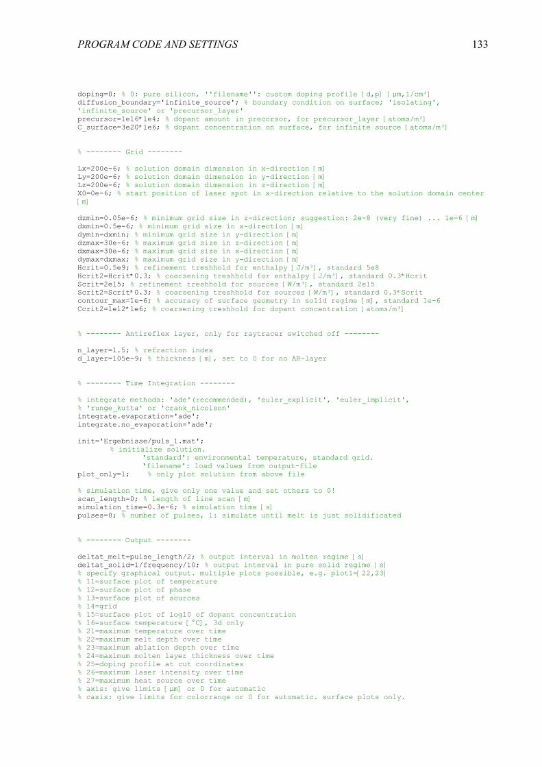
PROGRAM CODE AND SETTINGS
133
doping=0; % 0: pure silicon, ''filename'': custom doping profile [d,p] [µm,1/cm³] diffusion_boundary='infinite_source'; % boundary condition on surface; 'isolating', 'infinite_source' or 'precursor_layer' precursor=1e16*1e4; % dopant amount in precorsor, for precursor_layer [atoms/m²] C_surface=3e20*1e6; % dopant concentration on surface, for infinite source [atoms/m³] % -------- Grid -------- Lx=200e-6; % solution domain dimension in x-direction [m] Ly=200e-6; % solution domain dimension in y-direction [m] Lz=200e-6; % solution domain dimension in z-direction [m] X0=0e-6; % start position of laser spot in x-direction relative to the solution domain center [m] dzmin=0.05e-6; % minimum grid size in z-direction; suggestion: 2e-8 (very fine) ... 1e-6 [m] dxmin=0.5e-6; % minimum grid size in x-direction [m] dymin=dxmin; % minimum grid size in y-direction [m] dzmax=30e-6; % maximum grid size in z-direction [m] dxmax=30e-6; % maximum grid size in x-direction [m] dymax=dxmax; % maximum grid size in y-direction [m] Hcrit=0.5e9; % refinement treshhold for enthalpy [J/m³], standard 5e8 Hcrit2=Hcrit*0.3; % coarsening treshhold for enthalpy [J/m³], standard 0.3*Hcrit Scrit=2e15; % refinement treshhold for sources [W/m³], standard 2e15 Scrit2=Scrit*0.3; % coarsening treshhold for sources [W/m³], standard 0.3*Scrit contour_max=1e-6; % accuracy of surface geometry in solid regime [m], standard 1e-6 Ccrit2=1e12*1e6; % coarsening treshhold for dopant concentration [atoms/m³] % -------- Antireflex layer, only for raytracer switched off -------- n_layer=1.5; % refraction index d_layer=105e-9; % thickness [m], set to 0 for no AR-layer % -------- Time Integration -------- % integrate methods: 'ade'(recommended), 'euler_explicit', 'euler_implicit', % 'runge_kutta' or 'crank_nicolson' integrate.evaporation='ade'; integrate.no_evaporation='ade'; init='Ergebnisse/puls_1.mat';
% initialize solution. 'standard': environmental temperature, standard grid. 'filename': load values from output-file
plot_only=1; % only plot solution from above file % simulation time, give only one value and set others to 0! scan_length=0; % length of line scan [m] simulation_time=0.3e-6; % simulation time [s] pulses=0; % number of pulses, 1: simulate until melt is just solidificated % -------- Output -------- deltat_melt=pulse_length/2; % output interval in molten regime [s] deltat_solid=1/frequency/10; % output interval in pure solid regime [s] % specify graphical output. multiple plots possible, e.g. plot1=[22,23] % 11=surface plot of temperature % 12=surface plot of phase % 13=surface plot of sources % 14=grid % 15=surface plot of log10 of dopant concentration % 16=surface temperature [°C], 3d only % 21=maximum temperature over time % 22=maximum melt depth over time % 23=maximum ablation depth over time % 24=maximum molten layer thickness over time % 25=doping profile at cut coordinates % 26=maximum laser intensity over time % 27=maximum heat source over time % axis: give limits [µm] or 0 for automatic % caxis: give limits for colorrange or 0 for automatic. surface plots only.

PROGRAM CODE AND SETTINGS
134
% upper left axis: plot1=[22,23]; axis1=[]; caxis1=[]; % upper right axis: plot2=31; axis2=[70 130 70 130 -2 2]; caxis2=[]; % lower left axis: plot3=12; axis3=[70 130 0 3]; caxis3=[]; % lower right axis: plot4=15; axis4=[70 130 0 3]; caxis4=[16 21]; plot_cut=[100,100,0]; % cut coordinates for graphical output [X Y Z] [µm] plot_orientation='y'; % 3d only: specify coordinates of plot surface normal 'x', 'y' or 'z' % make movies from the following plots, [] means no movies movies=[]; % figure width x height. Standard [998 786], [1265 1050]. [1586 1405] for 480x480 nodisplay video; figure_size=[998 786]; % temperatures Tenv=300; % environmental temperature [K] Tstart=Tenv; % starting temperature [K] Tjet=Tenv; % temperature of liquid jet [K] % -------- Start parameter sweep -------- param=[]; % parameter values, [] means no parameter sweep parameter_plot=[]; for i_param=1:max(1,length(param)) if length(param)>0 fluence=param(i_param); % identify parameter here mkdir(['Ergebnisse/',num2str(param(i_param))]); end simulate; parameter_plot=[parameter_plot,melt_duration]; % output variable to plot over parameter for i=movies for p=1:per save Ergebnisse/movie_number.mat i p !./make_mpg end !cat Ergebnisse/*.mpg >Ergebnisse/out.mpg movefile('Ergebnisse/out.mpg',['Ergebnisse/movie',num2str(i),'.mpg2']); delete('Ergebnisse/*.mpg'); end for i=movies movefile(['Ergebnisse/movie',num2str(i),'.mpg2'],['Ergebnisse/movie',num2str(i),'.mpg']); end if length(param)>0 movefile('Ergebnisse/*.mat',['Ergebnisse/',num2str(param(i_param))]); movefile('Ergebnisse/*.fig',['Ergebnisse/',num2str(param(i_param))]); if length(movies)>0 movefile('Ergebnisse/*.mov',['Ergebnisse/',num2str(param(i_param))]); movefile('Ergebnisse/*.mpg',['Ergebnisse/',num2str(param(i_param))]); end end end if length(param)>1 figure; plot(param,parameter_plot); end
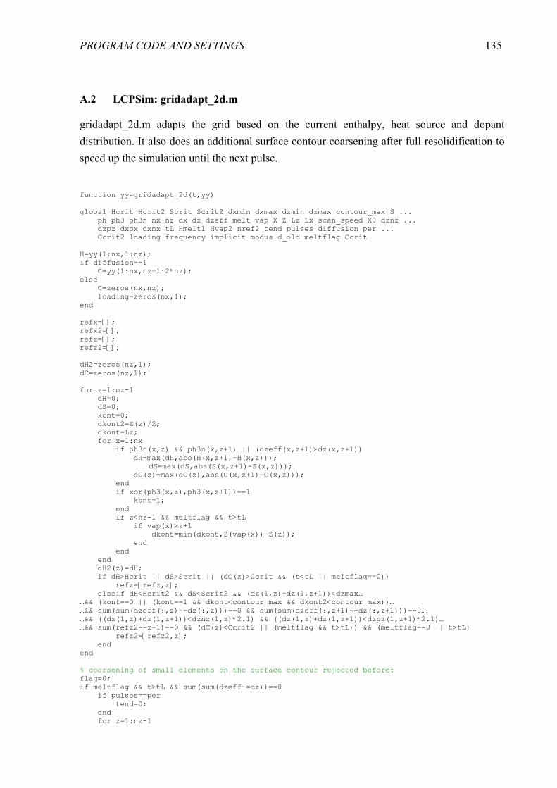
PROGRAM CODE AND SETTINGS
135
A.2 LCPSim: gridadapt_2d.m
gridadapt_2d.m adapts the grid based on the current enthalpy, heat source and dopant distribution. It also does an additional surface contour coarsening after full resolidification to speed up the simulation until the next pulse.
function yy=gridadapt_2d(t,yy) global Hcrit Hcrit2 Scrit Scrit2 dxmin dxmax dzmin dzmax contour_max S ... ph ph3 ph3n nx nz dx dz dzeff melt vap X Z Lz Lx scan_speed X0 dznz ... dzpz dxpx dxnx tL Hmelt1 Hvap2 nref2 tend pulses diffusion per ... Ccrit2 loading frequency implicit modus d_old meltflag Ccrit H=yy(1:nx,1:nz); if diffusion==1 C=yy(1:nx,nz+1:2*nz); else C=zeros(nx,nz); loading=zeros(nx,1); end refx=[]; refx2=[]; refz=[]; refz2=[]; dH2=zeros(nz,1); dC=zeros(nz,1); for z=1:nz-1 dH=0; dS=0; kont=0; dkont2=Z(z)/2; dkont=Lz; for x=1:nx if ph3n(x,z) && ph3n(x,z+1) || (dzeff(x,z+1)>dz(x,z+1)) dH=max(dH,abs(H(x,z+1)-H(x,z))); dS=max(dS,abs(S(x,z+1)-S(x,z))); dC(z)=max(dC(z),abs(C(x,z+1)-C(x,z))); end if xor(ph3(x,z),ph3(x,z+1))==1 kont=1; end if z<nz-1 && meltflag && t>tL if vap(x)>z+1 dkont=min(dkont,Z(vap(x))-Z(z)); end end end dH2(z)=dH; if dH>Hcrit || dS>Scrit || (dC(z)>Ccrit && (t<tL || meltflag==0)) refz=[refz,z]; elseif dH<Hcrit2 && dS<Scrit2 && (dz(1,z)+dz(1,z+1))<dzmax… …&& (kont==0 || (kont==1 && dkont<contour_max && dkont2<contour_max))… …&& sum(sum(dzeff(:,z)~=dz(:,z)))==0 && sum(sum(dzeff(:,z+1)~=dz(:,z+1)))==0… …&& ((dz(1,z)+dz(1,z+1))<dznz(1,z)*2.1) && ((dz(1,z)+dz(1,z+1))<dzpz(1,z+1)*2.1)… …&& sum(refz2==z-1)==0 && (dC(z)<Ccrit2 || (meltflag && t>tL)) && (meltflag==0 || t>tL) refz2=[refz2,z]; end end % coarsening of small elements on the surface contour rejected before: flag=0; if meltflag && t>tL && sum(sum(dzeff~=dz))==0 if pulses==per tend=0; end for z=1:nz-1

PROGRAM CODE AND SETTINGS
136
if dz(1,z)<contour_max && flag==0 if z>1 if dz(1,z-1)<dz(1,z+1) if sum(refz2==z-2)==0 && sum(refz==z-2)==0 && sum(refz==z-1)==0… … && dH2(z-1)<Hcrit2 refz2=[refz2,z-1]; flag=1; end elseif sum(refz2==z-1)==0 && sum(refz==z-1)==0 && sum(refz==z)==0… … && dH2(z)<Hcrit2 refz2=[refz2,z]; flag=1; end elseif sum(refz2==z-1)==0 && sum(refz==z-1)==0 && sum(refz==z)==0 && dH2(z)<Hcrit2 refz2=[refz2,z]; flag=1; end end end end refz=sort(refz); refz2=sort(refz2); for i=length(refz2):-1:1 if sum(refz2(i)==refz+1)~=0 || sum(refz2(i)==refz-1)~=0 || sum(refz2(i)==refz2)>1 refz2(i)=[]; end end if strcmp(modus,'cw') nxm=sum(X<(Lx/2+scan_speed*t)); else nxm=sum(X<(Lx/2+scan_speed*(per-1)/frequency+X0)); end for x=[nxm-1:-1:1,nxm:nx-1] dH=0; dS=0; dC=0; kont=0; for z=1:nz if ph3n(x,z) && ph3n(x+1,z) dH=max(dH,abs(H(x+1,z)-H(x,z))); dS=max(dS,abs(S(x+1,z)-S(x,z))); dC=max(dC,abs(C(x+1,z)-C(x,z))); end if xor(ph3(x,z),ph3(x+1,z))==1 || dzeff(x,z)~=dz(x,z) || dzeff(x+1,z)~=dz(x+1,z) kont=1; end end if dH>Hcrit || dS>Scrit || (dC>Ccrit && (t<tL || meltflag==0)) refx=[refx,x]; elseif (dH<Hcrit2 && dS<Scrit2) && (dx(x,1)+dx(x+1,1))<dxmax && kont==0… … && sum(refx2==x-1)==0 && sum(refx2==x+1)==0 && (dx(x,1)+dx(x+1,1))<dxnx(x,1)*2.1… … && (dx(x,1)+dx(x+1,1))<dxpx(x+1,1)*2.1 && dC<Ccrit2 && (meltflag==0 || t>tL) refx2=[refx2,x]; end end refx=sort(refx); refx2=sort(refx2); for i=length(refx2):-1:1 if sum(refx2(i)==refx+1)~=0 || sum(refx2(i)==refx-1)~=0 refx2(i)=[]; end end %%%%%%%%%%%%%%%%%%%%%%%%%%%%%%%%%%%%%%%%%%% if (nref2==50 && implicit==0) || (nref2==2 && implicit==1) refx=[]; nref2=0; else refx2=[];

PROGRAM CODE AND SETTINGS
137
nref2=nref2+1; end if t>tL && meltflag %sum(sum((H.*ph3n)>Hvap1))==0 for z=1:nz-1 if (sum(sum(dzeff(:,z)~=dz(:,z)))>0) for x=1:nx if dzeff(x,z)<dz(x,z)/2 H(x,z)=2*Hvap2; C(x,z)=1; else H(x,z)=H(x,z)*dzeff(x,z)/dz(x,z); end end dzeff(:,z)=dz(:,z); end end end for i=length(refz2):-1:1 z=refz2(i); for x=1:nx if ph3(x,z) && ph3n(x,z+1) && dz(1,z)>=dz(1,z+1) H(x,z)=2*Hvap2; C(x,z)=1; elseif ph3(x,z) && ph3n(x,z+1) && dz(1,z)<dz(1,z+1) H(x,z)=H(x,z+1); C(x,z)=C(x,z+1); else H(x,z)=(H(x,z)*dz(x,z)+H(x,z+1)*dz(x,z+1))/(dz(x,z)+dz(x,z+1)); C(x,z)=(C(x,z)*dz(x,z)+C(x,z+1)*dz(x,z+1))/(dz(x,z)+dz(x,z+1)); end end H(:,z+1)=[]; C(:,z+1)=[]; dz(:,z)=dz(1,z)+dz(1,z+1); dz(:,z+1)=[]; dx(:,z+1)=[]; dzeff(:,z+1)=[]; dzeff(:,z)=dz(:,z); nz=nz-1; refz=refz-(refz>=z); end for i=length(refz):-1:1 z=refz(i)+1; st=zeros(nx,1); st=(H(:,z)-H(:,z-1))/(dz(1,z-1)+dz(1,z))*2; st_d=(d_old(:,z)-d_old(:,z-1))/(dz(1,z-1)+dz(1,z))*2; st=st.*(H(:,z)<Hvap2).*(H(:,z-1)<Hvap2); st_d=st_d.*(H(:,z)<Hvap2).*(H(:,z-1)<Hvap2); if dz(1,z)/2>dzmin && dzeff(1,z)==dz(1,z) dz(:,z+2:nz+1)=dz(:,z+1:nz); dz(:,z+1)=dz(1,z)-min(dz(1,z)/2,dz(1,z-1)); dz(:,z)=dz(1,z)-dz(1,z+1); H(:,z+2:nz+1)=H(:,z+1:nz); Halt=H(:,z); H(:,z)=Halt-dz(1,z+1)/2*st; H(:,z+1)=Halt+dz(1,z)/2*st; C(:,z+2:nz+1)=C(:,z+1:nz); Calt=C(:,z); C(:,z)=Calt; C(:,z+1)=Calt; if (sum(H(:,z)<0)+sum(H(:,z+1)<0))~=0 H(:,z)=Halt; H(:,z+1)=Halt; end dx(:,nz+1)=dx(:,1); dzeff(:,z+2:nz+1)=dzeff(:,z+1:nz); dzeff(:,z:z+1)=dz(:,z:z+1); nz=nz+1; end z=z-1; if dz(1,z)/2>dzmin && dzeff(1,z)==dz(1,z) && sum(refz==z-1)==0 dz(:,z+2:nz+1)=dz(:,z+1:nz);

PROGRAM CODE AND SETTINGS
138
dz(:,z+1)=min(dz(1,z)/2,dz(1,z+1)); dz(:,z)=dz(1,z)-dz(1,z+1); H(:,z+2:nz+1)=H(:,z+1:nz); Halt=H(:,z); d_oldalt=d_old(:,z); H(:,z)=Halt-dz(1,z+1)/2*st; H(:,z+1)=Halt+dz(1,z)/2*st; C(:,z+2:nz+1)=C(:,z+1:nz); Calt=C(:,z); C(:,z)=Calt; C(:,z+1)=Calt; if (sum(H(:,z)<0)+sum(H(:,z+1)<0))~=0 H(:,z)=Halt; H(:,z+1)=Halt; end dx(:,nz+1)=dx(:,1); dzeff(:,z+2:nz+1)=dzeff(:,z+1:nz); dzeff(:,z:z+1)=dz(:,z:z+1); nz=nz+1; end end for i=length(refx2):-1:1 x=refx2(i); H(x,:)=(H(x,:)*dx(x,1)+H(x+1,:)*dx(x+1,1))/(dx(x,1)+dx(x+1,1)); H(x+1,:)=[]; C(x,:)=(C(x,:)*dx(x,1)+C(x+1,:)*dx(x+1,1))/(dx(x,1)+dx(x+1,1)); C(x+1,:)=[]; loading(x)=(loading(x)*dx(x,1)+loading(x+1)*dx(x+1,1))/(dx(x,1)+dx(x+1,1)); loading(x+1)=[]; dx(x,:)=dx(x,1)+dx(x+1,1); dx(x+1,:)=[]; dz(x+1,:)=[]; dzeff(x,:)=(dzeff(x,:)+dzeff(x+1,:))/2; dzeff(x+1,:)=[]; nx=nx-1; refx=refx-(refx>=x); end for i=length(refx):-1:1 x=refx(i)+1; if dx(x,1)/2>dxmin dx(x+2:nx+1,:)=dx(x+1:nx,:); dx(x+1,:)=dx(x,1)-min(dx(x,1)/2,dx(x-1,1)); dx(x,:)=dx(x,1)-dx(x+1,1); H(x+2:nx+1,:)=H(x+1:nx,:); Halt=H(x,:); H(x,:)=Halt;%-dx(x+1,1)/2*st; H(x+1,:)=Halt;%+dx(x,1)/2*st; loading(x+2:nx+1)=loading(x+1:nx); loadingold=loading(x); loading(x)=loadingold; loading(x+1)=loadingold; C(x+2:nx+1,:)=C(x+1:nx,:); Calt=C(x,:); C(x,:)=Calt; C(x+1,:)=Calt; dz(nx+1,:)=dz(1,:); dzeff(x+2:nx+1,:)=dzeff(x+1:nx,:); dzeff(x+1,:)=dzeff(x,:); nx=nx+1; end x=x-1; if dx(x,1)/2>dxmin && sum(refx==x-1)==0 dx(x+2:nx+1,:)=dx(x+1:nx,:); dx(x+1,:)=min(dx(x,1)/2,dx(x+1,1)); dx(x,:)=dx(x,1)-dx(x+1,1); H(x+2:nx+1,:)=H(x+1:nx,:); Halt=H(x,:); H(x,:)=Halt;%-dx(x+1,1)/2*st; H(x+1,:)=Halt;%+dx(x,1)/2*st; loading(x+2:nx+1)=loading(x+1:nx); loadingold=loading(x); loading(x)=loadingold; loading(x+1)=loadingold;

PROGRAM CODE AND SETTINGS
139
C(x+2:nx+1,:)=C(x+1:nx,:); Calt=C(x,:); C(x,:)=Calt; C(x+1,:)=Calt; dz(nx+1,:)=dz(1,:); dzeff(x+2:nx+1,:)=dzeff(x+1:nx,:); dzeff(x+1,:)=dzeff(x,:); nx=nx+1; end end %%%%%%%%%%%%%%%%%%%%%%%%%%%%%%%%%% X=dx(1,1)/2; for x=2:nx X=[X,X(length(X))+(dx(x,1)+dx(x-1,1))/2]; end Z=dz(1,1)/2; for z=2:nz Z=[Z,Z(length(Z))+(dz(1,z)+dz(1,z-1))/2]; end if diffusion==0 yy=H; else yy=[H,C]; end
A.3 LCPSim: ade_2d.m
This is the 2d axial symmetric version of the ADE algorithm to integrate over one time step.
function yy=ade_2d(t,yy) global T ph ph3 ph3n Hmelt1 Hmelt2 nx nz Tmelt Tenv dt dzeff dx dz dzmax ... H surfx surfz melt vap S Sneu qz qznx qzpx Tvap1 Hvap11 Hvap21 r ... rnx rpx dxnx dxpx dznz dzpz lanx2 lapx2 lanz2 lapz2 Tnx Tpx Tnz Tpz ... temperature Hvap2 Hvap1 LHvap Tvap dtalt evap_model p_jet rcl aT bT ... cT dT eT H_old T_old ph_old d_old meltflag X Z density_change H=yy; Sneu=S.*dx.*dzeff; T_old=T; ph_old=ph; lanx2=lanx2.*(surfx~=-1); lapx2=lapx2.*(surfx~=1); lanz2=lanz2.*(surfz~=-1); lapz2=lapz2.*(surfz~=1); Jpx=min(1,qzpx./qz)*2.*(Tpx-T)./(dx+dxpx).*lapx2.*rpx./r.*dzeff; Jnx=min(1,qznx./qz)*2.*(T-Tnx)./(dx+dxnx).*lanx2.*rnx./r.*dzeff; Jpz=2*(Tpz-T)./(dzeff+dzpz).*lapz2.*dx; Jnz=2*(T-Tnz)./(dzeff+dznz).*lanz2.*dx; U=H; T1nx=Tnx; T1nz=Tnz; T1px=Tpx; T1pz=Tpz; stab=1e-1; stab2=1e-1; stab3=1e-1; lazx=lanz2.*dx./(dzeff+dznz); laxz=min(1,qznx./qz).*lanx2.*dzeff./(dx+dxnx).*rnx./r; for x=1:nx for z=1:nz
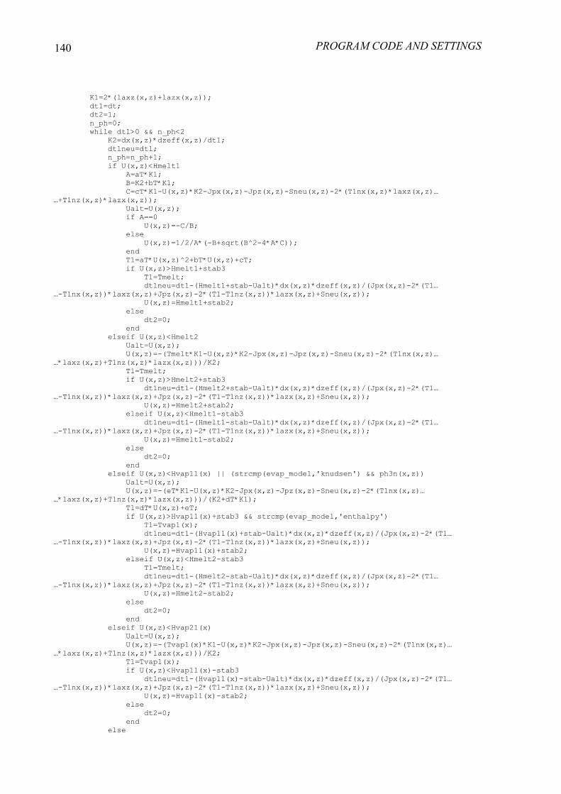
PROGRAM CODE AND SETTINGS
140
K1=2*(laxz(x,z)+lazx(x,z)); dt1=dt; dt2=1; n_ph=0; while dt1>0 && n_ph<2 K2=dx(x,z)*dzeff(x,z)/dt1; dt1neu=dt1; n_ph=n_ph+1; if U(x,z)<Hmelt1 A=aT*K1; B=K2+bT*K1; C=cT*K1-U(x,z)*K2-Jpx(x,z)-Jpz(x,z)-Sneu(x,z)-2*(T1nx(x,z)*laxz(x,z)… …+T1nz(x,z)*lazx(x,z)); Ualt=U(x,z); if A==0 U(x,z)=-C/B; else U(x,z)=1/2/A*(-B+sqrt(B^2-4*A*C)); end T1=aT*U(x,z)^2+bT*U(x,z)+cT; if U(x,z)>Hmelt1+stab3 T1=Tmelt; dt1neu=dt1-(Hmelt1+stab-Ualt)*dx(x,z)*dzeff(x,z)/(Jpx(x,z)-2*(T1… …-T1nx(x,z))*laxz(x,z)+Jpz(x,z)-2*(T1-T1nz(x,z))*lazx(x,z)+Sneu(x,z)); U(x,z)=Hmelt1+stab2; else dt2=0; end elseif U(x,z)<Hmelt2 Ualt=U(x,z); U(x,z)=-(Tmelt*K1-U(x,z)*K2-Jpx(x,z)-Jpz(x,z)-Sneu(x,z)-2*(T1nx(x,z)… …*laxz(x,z)+T1nz(x,z)*lazx(x,z)))/K2; T1=Tmelt; if U(x,z)>Hmelt2+stab3 dt1neu=dt1-(Hmelt2+stab-Ualt)*dx(x,z)*dzeff(x,z)/(Jpx(x,z)-2*(T1… …-T1nx(x,z))*laxz(x,z)+Jpz(x,z)-2*(T1-T1nz(x,z))*lazx(x,z)+Sneu(x,z)); U(x,z)=Hmelt2+stab2; elseif U(x,z)<Hmelt1-stab3 dt1neu=dt1-(Hmelt1-stab-Ualt)*dx(x,z)*dzeff(x,z)/(Jpx(x,z)-2*(T1… …-T1nx(x,z))*laxz(x,z)+Jpz(x,z)-2*(T1-T1nz(x,z))*lazx(x,z)+Sneu(x,z)); U(x,z)=Hmelt1-stab2; else dt2=0; end elseif U(x,z)<Hvap11(x) || (strcmp(evap_model,'knudsen') && ph3n(x,z)) Ualt=U(x,z); U(x,z)=-(eT*K1-U(x,z)*K2-Jpx(x,z)-Jpz(x,z)-Sneu(x,z)-2*(T1nx(x,z)… …*laxz(x,z)+T1nz(x,z)*lazx(x,z)))/(K2+dT*K1); T1=dT*U(x,z)+eT; if U(x,z)>Hvap11(x)+stab3 && strcmp(evap_model,'enthalpy') T1=Tvap1(x); dt1neu=dt1-(Hvap11(x)+stab-Ualt)*dx(x,z)*dzeff(x,z)/(Jpx(x,z)-2*(T1… …-T1nx(x,z))*laxz(x,z)+Jpz(x,z)-2*(T1-T1nz(x,z))*lazx(x,z)+Sneu(x,z)); U(x,z)=Hvap11(x)+stab2; elseif U(x,z)<Hmelt2-stab3 T1=Tmelt; dt1neu=dt1-(Hmelt2-stab-Ualt)*dx(x,z)*dzeff(x,z)/(Jpx(x,z)-2*(T1… …-T1nx(x,z))*laxz(x,z)+Jpz(x,z)-2*(T1-T1nz(x,z))*lazx(x,z)+Sneu(x,z)); U(x,z)=Hmelt2-stab2; else dt2=0; end elseif U(x,z)<Hvap21(x) Ualt=U(x,z); U(x,z)=-(Tvap1(x)*K1-U(x,z)*K2-Jpx(x,z)-Jpz(x,z)-Sneu(x,z)-2*(T1nx(x,z)… …*laxz(x,z)+T1nz(x,z)*lazx(x,z)))/K2; T1=Tvap1(x); if U(x,z)<Hvap11(x)-stab3 dt1neu=dt1-(Hvap11(x)-stab-Ualt)*dx(x,z)*dzeff(x,z)/(Jpx(x,z)-2*(T1… …-T1nx(x,z))*laxz(x,z)+Jpz(x,z)-2*(T1-T1nz(x,z))*lazx(x,z)+Sneu(x,z)); U(x,z)=Hvap11(x)-stab2; else dt2=0; end else

PROGRAM CODE AND SETTINGS
141
dt2=0; T1=Tvap1(x); end dt1=dt1neu; if dt2==0 dt1=0; end end if x~=nx T1nx(x+1,z)=T1; end if z~=nz T1nz(x,z+1)=T1; end end end V=H; lazx=lapz2.*dx./(dzeff+dzpz); laxz=min(1,qzpx./qz).*lapx2.*dzeff./(dx+dxpx).*rpx./r; for x=nx:-1:1 for z=nz:-1:1 K1=2*(laxz(x,z)+lazx(x,z)); dt1=dt; dt2=1; n_ph=0; while dt1>0 && n_ph<2 K2=dx(x,z)*dzeff(x,z)/dt1; dt1neu=dt1; n_ph=n_ph+1; if V(x,z)<Hmelt1 A=aT*K1; B=K2+bT*K1; C=cT*K1-V(x,z)*K2+Jnx(x,z)+Jnz(x,z)-Sneu(x,z)-2*(T1px(x,z)*laxz(x,z)… …+T1pz(x,z)*lazx(x,z)); Valt=V(x,z); if A==0 V(x,z)=-C/B; else V(x,z)=1/2/A*(-B+sqrt(B^2-4*A*C)); end T1=aT*V(x,z)^2+bT*V(x,z)+cT; if V(x,z)>Hmelt1+stab3 T1=Tmelt; dt1neu=dt1-(Hmelt1+stab-Valt)*dx(x,z)*dzeff(x,z)/(-Jnx(x,z)-2*(T1… …-T1px(x,z))*laxz(x,z)-Jnz(x,z)-2*(T1-T1pz(x,z))*lazx(x,z)+Sneu(x,z)); V(x,z)=Hmelt1+stab2; else dt2=0; end elseif V(x,z)<Hmelt2 Valt=V(x,z); V(x,z)=-(Tmelt*K1-V(x,z)*K2+Jnx(x,z)+Jnz(x,z)-Sneu(x,z)-2*(T1px(x,z)… …*laxz(x,z)+T1pz(x,z)*lazx(x,z)))/K2; T1=Tmelt; if V(x,z)>Hmelt2+stab3 dt1neu=dt1-(Hmelt2+stab-Valt)*dx(x,z)*dzeff(x,z)/(-Jnx(x,z)-2*(T1… …-T1px(x,z))*laxz(x,z)-Jnz(x,z)-2*(T1-T1pz(x,z))*lazx(x,z)+Sneu(x,z)); V(x,z)=Hmelt2+stab2; elseif V(x,z)<Hmelt1-stab3 dt1neu=dt1-(Hmelt1-stab-Valt)*dx(x,z)*dzeff(x,z)/(-Jnx(x,z)-2*(T1… …-T1px(x,z))*laxz(x,z)-Jnz(x,z)-2*(T1-T1pz(x,z))*lazx(x,z)+Sneu(x,z)); V(x,z)=Hmelt1-stab2; else dt2=0; end elseif V(x,z)<Hvap11(x) || (strcmp(evap_model,'knudsen') && ph3n(x,z)) Valt=V(x,z); V(x,z)=-(eT*K1-V(x,z)*K2+Jnx(x,z)+Jnz(x,z)-Sneu(x,z)-2*(T1px(x,z)… …*laxz(x,z)+T1pz(x,z)*lazx(x,z)))/(K2+dT*K1); T1=dT*V(x,z)+eT; if V(x,z)>Hvap11(x)+stab3 && strcmp(evap_model,'enthalpy') T1=Tvap1(x); dt1neu=dt1-(Hvap11(x)+stab-Valt)*dx(x,z)*dzeff(x,z)/(-Jnx(x,z)-2*(T1… …-T1px(x,z))*laxz(x,z)-Jnz(x,z)-2*(T1-T1pz(x,z))*lazx(x,z)+Sneu(x,z)); V(x,z)=Hvap11(x)+stab2;
PROGRAM CODE AND SETTINGS
142
elseif V(x,z)<Hmelt2-stab3 T1=Tmelt; dt1neu=dt1-(Hmelt2-stab-Valt)*dx(x,z)*dzeff(x,z)/(-Jnx(x,z)-2*(T1… …-T1px(x,z))*laxz(x,z)-Jnz(x,z)-2*(T1-T1pz(x,z))*lazx(x,z)+Sneu(x,z)); V(x,z)=Hmelt2-stab2; else dt2=0; end elseif V(x,z)<Hvap21(x) Valt=V(x,z); V(x,z)=-(Tvap1(x)*K1-V(x,z)*K2+Jnx(x,z)+Jnz(x,z)-Sneu(x,z)-2*(T1px(x,z)… …*laxz(x,z)+T1pz(x,z)*lazx(x,z)))/K2; T1=Tvap1(x); if V(x,z)<Hvap11(x)-stab3 dt1neu=dt1-(Hvap11(x)-stab-Valt)*dx(x,z)*dzeff(x,z)/(-Jnx(x,z)-2*(T1… …-T1px(x,z))*laxz(x,z)-Jnz(x,z)-2*(T1-T1pz(x,z))*lazx(x,z)+Sneu(x,z)); V(x,z)=Hvap11(x)-stab2; else dt2=0; end else dt2=0; T1=Tvap1(x); end dt1=dt1neu; if dt2==0 dt1=0; end end if x~=1 T1px(x-1,z)=T1; end if z~=1 T1pz(x,z-1)=T1; end end end H=(U+V)/2; [T,H,ph,dzeff]=temperature(H,nx,nz,dzeff,ph,dz,t); melt=max(melt,vap); ph3=ph==3; ph3n=ph<3; H=H.*ph3n+2*Hvap2*ph3; yy=H;
A.4 LCPSim: sims.m
This post processing algorithm corresponds to the SIMS measurement method, where the atom concentration is averaged over the ion beam diameter.
clear all; load('Ergebnisse/puls_39.mat'); % Define centre, diameter and depth of SIMS Xsims=130e-6; Ysims=100e-6; Dsims=10e-6; tsims=3e-6; nsims=100; A=zeros(nx,ny); Zsims=zeros(nx,ny,nz); Zmin=1; for x=1:nx for y=1:ny if abs(X(x)-Xsims)<Dsims/2 && abs(Y(y)-Ysims)<Dsims/2

PROGRAM CODE AND SETTINGS
143
A(x,y)=dx(x,1,1)*dy(1,y,1); z=sum(ph(x,y,:)==3)+1; Z1=Z(z)+dz(1,1,z)/2-dzeff(x,y,z); Zmin=min(Zmin,Z1); for z=1:nz Zsims(x,y,z)=Z(z)-dz(1,1,z)/2-Z1; end Zsims(x,y,z)=0; end end end Csims=ones(1,nz); for z=1:nz Csims(z)=sum(sum(C(:,:,z).*A.*dzeff(:,:,z)))/dz(1,1,z)/sum(sum(A)); end Zsims2=0:tsims/nsims:tsims; Csims2=ones(1,nsims+1); for i=1:nsims+1 Zs=Zsims2(i); Csum=0; for x=1:nx for y=1:ny if abs(X(x)-Xsims)<Dsims/2 && abs(Y(y)-Ysims)<Dsims/2 Csum=Csum+A(x,y)*C(x,y,sum(Zsims(x,y,:)<=Zs)); end end end Csims2(i)=Csum/sum(sum(A)); end Cs=ones(1,nz); xcut=sum(X<Xsims); ycut=sum(Y<Ysims); z=sum(ph(xcut,ycut,:)==3)+1; Zsmin=Z(z)+dz(1,1,z)/2-dzeff(xcut,ycut,z); Cs(1:nz)=C(xcut,ycut,:); semilogy(Zsims2*1e6,Csims2*1e-6); xlabel('distance to surface [µm]'); ylabel('C [atoms/m³]'); axis([0 1.5 1e16 1e21]);
A.5 Fluent: Fluent C-code for UDFs #define min(x1,x2) ((x1) > (x2))? (x2):(x1) #define max(x1,x2) ((x1) > (x2))? (x1):(x2) #define Tmelt1 1680 #define Tmelt2 1690 #define Hmelt1 3.3678e9 #define Hmelt2 7.4978e9 int melt = 0; DEFINE_ADJUST(uds_temperature_mixture,d) { Thread *t,*t1,*t2,*t0; cell_t c; real TS, HS; Domain *pDomain = DOMAIN_SUB_DOMAIN(d,2); { Alloc_Storage_Vars(pDomain,SV_VOF_RG,SV_VOF_G,SV_NULL); Scalar_Reconstruction(pDomain, SV_VOF,-1,SV_VOF_RG,NULL); Scalar_Derivatives(pDomain,SV_VOF,-1,SV_VOF_G,SV_VOF_RG,Vof_Deriv_Accumulate); } melt = 0; thread_loop_c(t,d) { t0 = THREAD_SUB_THREAD(t,0); t1 = THREAD_SUB_THREAD(t,1);

PROGRAM CODE AND SETTINGS
144
t2 = THREAD_SUB_THREAD(t,2); begin_c_loop(c,t) C_UDMI(c,t,0) = C_VOF_G(c,t2)[0]; C_UDMI(c,t,1) = C_VOF_G(c,t2)[1]; C_UDMI(c,t,6) = 0; HS = C_UDSI(c,t2,1); if (HS<Hmelt1) { TS = min(Tmelt1,98.06+5.512e-7*HS-2.375e-17*pow(HS,2)); C_UDMI(c,t,6) = 5.512e-7-2*2.375e-17*HS; } else if (HS<Hmelt2) { TS = Tmelt1+(Tmelt2-Tmelt1)*(HS-Hmelt1)/(Hmelt2-Hmelt1); melt = 1; C_UDMI(c,t,6) = (Tmelt2-Tmelt1)/(Hmelt2-Hmelt1); } else { TS = max(Tmelt2,HS*4.1118e-7-1.3980e+3); melt = 1; C_UDMI(c,t,6) = 4.1118e-7; } C_T(c,t) = C_UDSI(c,t1,0)*C_VOF(c,t1)+TS*C_VOF(c,t2)+(1-C_VOF(c,t1)-C_VOF(c,t2))*300; if (C_VOF(c,t2)>0) { C_T(c,t) = TS; } C_UDMI(c,t,2) = 0; C_UDMI(c,t,3) = 0; C_UDMI(c,t,4) = 0; C_UDMI(c,t,5) = 0; end_c_loop(c,t) } Free_Storage_Vars(pDomain,SV_VOF_RG,SV_VOF_G,SV_NULL); } DEFINE_DIFFUSIVITY(uds_diffusity,c,t,i) { return C_K_L(c,t)/C_CP(c,t); } DEFINE_SOURCE(radial_solidfication_velocity,c,t,dS,eqn) { real source, b = 1, vof2; Thread *ts; ts = THREAD_SUB_THREAD(t,2); if (C_T(c,t)<Tmelt2 && C_VOF(c,ts)>0) { vof2 = min(1,10*C_VOF(c,ts)); if (C_T(c,t)>Tmelt1) { b = 1-vof2*(1-(C_T(c,t)-Tmelt1)/(Tmelt2-Tmelt1)); } else { b = 1-vof2; } source = -pow((1-b),2)/(pow(b,3)+0.001)*1e10*C_V(c,t); } else { source = 0; } dS[eqn] = source/C_V(c,t); return source; } DEFINE_SOURCE(axial_solidfication_velocity,c,t,dS,eqn) { real source, b = 1, vof2; Thread *ts; ts = THREAD_SUB_THREAD(t,2);

PROGRAM CODE AND SETTINGS
145
if (C_T(c,t)<Tmelt2 && C_VOF(c,ts)>0) { vof2 = min(1,10*C_VOF(c,ts)); if (C_T(c,t)>Tmelt1) { b = 1-vof2*(1-(C_T(c,t)-Tmelt1)/(Tmelt2-Tmelt1)); } else { b = 1-vof2; } source = -pow((1-b),2)/(pow(b,3)+0.001)*1e10*C_U(c,t); } else { source = 0; } dS[eqn] = source/C_U(c,t); return source; } DEFINE_SOURCE(latent_heat,c,t,dS,eqn) { real source = 0; real LH = 4.13e9; real Tmin, Tmax, T1, T2, Talt; dS[eqn] = 0; T2 = C_UDSI(c,t,1); T1 = C_UDSI_M1(c,t,1); if ((T2<=Tmelt2 && T2>=Tmelt1) || (T1<=Tmelt2 && T1>=Tmelt1) || (max(T1,T2)>Tmelt2… …&& min(T1,T2)<Tmelt1)) { Tmin = min(max(T2,Tmelt1),Tmelt2); Talt = T1; Tmax = min(max(Talt,Tmelt1),Tmelt2); source = -LH/(Tmelt2-Tmelt1)/C_CP(c,t)/CURRENT_TIMESTEP*(Tmin-Tmax-(Tmelt2-Tmelt1)/… …2/M_PI*(sin(2*M_PI*(Tmin-Tmelt1)/(Tmelt2-Tmelt1))-sin(2*M_PI*(Tmax-Tmelt1)/(Tmelt2… …-Tmelt1))))*C_VOF(c,t); dS[eqn] = -LH/(Tmelt2-Tmelt1)/CURRENT_TIMESTEP/C_CP(c,t)*(1-cos(2*M_PI*(Tmin-Tmelt1)… …/(Tmelt2-Tmelt1)))*C_VOF(c,t); } return source; } DEFINE_SOURCE(density_change,c,t2,dS,eqn) { real rho1 = 1430, rho2 = 1430, T1, T2; real Tm1, Tm2; real source; Thread *t = THREAD_SUPER_THREAD(t2); T1 = C_T_M1(c,t); T2 = C_T(c,t); Tm1 = Tmelt1; Tm2 = Tmelt2; if (T1<Tm1) { rho1 = 2330; } else if (T1<Tm2) { rho1 = 2330+210*(T1-Tm1)/(Tm2-Tm1); } else if (T1<4690) { rho1 = 2540-1110*(T1-Tm2)/(4690-Tm2); } if (T2<Tm1) {

PROGRAM CODE AND SETTINGS
146
rho2 = 2330; } else if (T2<Tm2) { rho2 = 2330+210*(T2-Tm1)/(Tm2-Tm1); } else if (T2<4690) { rho2 = 2540-1110*(T2-Tm2)/(4690-Tm2); } dS[eqn] = 0; source = (rho1-rho2)/CURRENT_TIMESTEP*C_VOF(c,t2); return source; } DEFINE_SOURCE(water_interface_heat_transfer,c,t2,dS,eqn) { real grad_vof, source, derivate, Ts, n1, n2; real dist, x1[ND_ND], x2[ND_ND], sp1, sp2, NV_VEC(A); Thread *t = THREAD_SUPER_THREAD(t2); Thread *t3 = THREAD_SUB_THREAD(t,2); Thread *tf, *tc1, *tc2, *tc13, *tc23, *tc12, *tc22, *tcx, *tcx2, *tcx3; face_t f; cell_t c1, c2, cx; int n; source = 0; derivate = 0; sp1 = 0; if (C_VOF(c,t2)>0.53) { C_CENTROID(x1,c,t); c_face_loop(c,t,n) { f = C_FACE(c,t,n); tf = C_FACE_THREAD(c,t,n); c1 = F_C0(f,tf); c2 = F_C1(f,tf); tc1 = THREAD_T0(tf); tc2 = THREAD_T1(tf); tc13 = THREAD_SUB_THREAD(tc1,2); tc12 = THREAD_SUB_THREAD(tc1,1); F_AREA(A,f,tf); n1 = pow(pow(C_UDMI(c,t,0),2)+pow(C_UDMI(c,t,1),2),0.5); n2 = pow(pow(A[0],2)+pow(A[1],2),0.5); sp2 = fabs(C_UDMI(c,t,0)*A[0]+C_UDMI(c,t,1)*A[1])/n1/n2; if (C_VOF(c1,tc13)>=0.47 && sp2>C_UDMI(c,t,4)) { tcx = THREAD_T0(tf); tcx2 = THREAD_SUB_THREAD(tc1,1); tcx3 = THREAD_SUB_THREAD(tc1,2); cx = F_C0(f,tf); C_UDMI(c,t,4) = sp2; sp1 = 1; } if (NULL != tc2) { tc23 = THREAD_SUB_THREAD(tc2,2); tc22 = THREAD_SUB_THREAD(tc2,1); if (C_VOF(c2,tc23)>=0.47 && sp2>C_UDMI(c,t,4)) { tcx = THREAD_T1(tf); tcx2 = THREAD_SUB_THREAD(tc2,1); tcx3 = THREAD_SUB_THREAD(tc2,2); cx = F_C1(f,tf); C_UDMI(c,t,4) = sp2; sp1 = 1; } } } if (sp1==1) { grad_vof = pow(pow(C_UDMI(c,t,0),2)+pow(C_UDMI(c,t,1),2),0.5)… …+pow(pow(C_UDMI(cx,tcx,0),2)+pow(C_UDMI(cx,tcx,1),2),0.5);

PROGRAM CODE AND SETTINGS
147
C_CENTROID(x2,cx,tcx); dist = pow(pow(x1[0]-x2[0],2)+pow(x1[1]-x2[1],2),0.5)*C_UDMI(c,t,4); Ts = C_T(cx,tcx); source = C_K_L(c,t2)*(Ts-C_UDSI(c,t2,0))*grad_vof/dist/(C_VOF(c,t2)-0.5+C_VOF(cx,tcx2)); derivate = -C_K_L(c,t2)*grad_vof/dist/(C_VOF(c,t2)-0.5+C_VOF(cx,tcx2)); C_UDMI(cx,tcx,2) = C_UDMI(cx,tcx,2)+source*C_VOLUME(c,t)/C_VOLUME(cx,tcx); C_UDMI(cx,tcx,3) = C_UDMI(cx,tcx,3)+derivate*C_VOLUME(c,t)/C_VOLUME(cx,tcx); C_UDMI(c,t,5) = source/grad_vof/(Ts-300); C_UDMI(cx,tcx,5) = source/grad_vof/(Ts-300); } } dS[eqn] = derivate/C_CP(c,t2); return source/C_CP(c,t2); } DEFINE_SOURCE(silicon_interface_heat_transfer,c,t3,dS,eqn) { Thread *t = THREAD_SUPER_THREAD(t3); dS[eqn] = C_UDMI(c,t,3)*C_R(c,t3)*C_UDMI(c,t,6); return -C_UDMI(c,t,2)*C_R(c,t3); } DEFINE_ON_DEMAND(run_matlab) { int flag = 0, step; real tim, offset, tim2; FILE *fp; char cp[FILENAME_MAX]; offset = RP_Get_Real("time_offset"); tim2 = CURRENT_TIME-offset; Message("offset = %e\nexport = %e\n",offset,tim2); getcwd(cp, sizeof(cp)); fp = fopen(strcat(cp,"/current_time.dat"),"w"); fprintf(fp,"%e\n",tim2); fclose(fp); step = RP_Get_Integer("time-step"); getcwd(cp, sizeof(cp)); fp = fopen(strcat(cp,"/current_step.dat"),"w"); fprintf(fp,"%d\n",step); fclose(fp); getcwd(cp, sizeof(cp)); fp = fopen(strcat(cp,"/current_timestep.dat"),"w"); fprintf(fp,"%e\n",CURRENT_TIMESTEP); fclose(fp); getcwd(cp, sizeof(cp)); fp = fopen(strcat(cp,"/fluent_status.dat"),"w"); fprintf(fp,"%d\n",1); fclose(fp); while (flag<2) { usleep(100000); getcwd(cp, sizeof(cp)); fp = fopen(strcat(cp,"/fluent_status.dat"),"r"); fscanf (fp,"%d",&flag); fclose(fp); } getcwd(cp, sizeof(cp)); fp = fopen(strcat(cp,"/current_time.dat"),"r"); fscanf(fp,"%lg",&tim); fclose(fp); tim2=tim+offset; RP_Set_Real("flow-time",tim2); Message("CURRENT_TIME = %e\n",CURRENT_TIME); }
A.6 Fluent: solver settings
The used solver settings for Fluent v. 6.3 are given for those different from the standard settings. These settings are also used for the coupled code.

PROGRAM CODE AND SETTINGS
148
description setting remarks
fixed time step size ns3.02.0 −
volume fraction discretization scheme
geometric reconstruction
to ensure the free surface to be one element sharp
water UDS discretization scheme third order muscle
lower order discretization gives bad results for free surface heat transfer
all other discretization schemes second order
UDS under relaxation factor 0.9
UDS convergence residual 75 −e similar to the energy residual
silicon viscosity for silicon below melting temperature sm
kg07.0 higher values causes divergence of pressure; lower values increase numerical movement of solid silicon

149
B List of symbols and abbreviations
symbol unit description
a volume fraction
A 2m area
b beam direction vector with unit length
c coefficients of the temperature – enthalpy relation
lc sm speed of light
pc )( KkgJ specific heat capacity
C 3−m species concentration
HC 2mJ constant for semi analytic surface enthalpy distribution
UC , VC constants for ADE expressions
d m thickness or diameter
D sm2 diffusion coefficient
E unit tensor
E J energy
f 1−s frequency or repetition rate
F 2mJ laser fluence
G gray value of CCD image
h sJ Planck constant
ht )( 2 KmW heat transfer coefficient
H 3mJ enthalpy
i imaginary unit
I 2mW laser light intensity

LIST OF SYMBOLS AND ABBREVIATIONS
150
symbol unit description
I 2mW spatial averaged laser light intensity
J 2mW heat flux
k negative imaginary part of refraction index, extinction coefficient
rk )(3 smolm kinetic rate constant
Bk KJ Boltzmann constant
K )( KmW heat conductivity
l m length
L 3mJ latent heat
molL molJ molar latent heat
am kg atom mass
M molkg molar mass
n real part of refraction index
*n complex refraction index
n surface normal vector with unit length
n& 1−s removal rate
np multiphase phase count
nx element count in x coordinate
ny element count in y coordinate
nz element count in z coordinate
AN 1−mol Avogadro constant
p 2mN static pressure
P W laser power
r m radial coordinate, distance from centre of axial symmetry
*r complex amplitude reflectivity

LIST OF SYMBOLS AND ABBREVIATIONS
151
symbol unit description
R reflectivity
mR )( molKJ molar gas constant
S source term, unit with respect to the corresponding equation
t s time
T K temperature
U ( )3mJ forward part in ADE algorithm, unit of enthalpy for heat transport equation
v sm velocity vector
V 3m ; ( )3mJ volume; backward part in ADE algorithm, unit of enthalpy for heat transport equation
α 1−m absorption coefficient
β liquid fraction
δ relative path enlargement
fδ optical path difference
rHΔ molJ reaction enthalpy
tΔ s time step size
xΔ m element size in x coordinate
yΔ m element size in y coordinate
zΔ m element size in z coordinate
ε relative permittivity
*ε complex relative permittivity
0ε )( mVsA dielectric constant
Tε relative emissivity
Φ sm general flux
dΦ quantum efficiency

LIST OF SYMBOLS AND ABBREVIATIONS
152
symbol unit description
ϕ ° angle
Γ sm2 general diffusivity
γ 1−s collision rate
Κ sm kinetic rate constant
λ m wavelength
μ 2msN molecular viscosity
ρ 3mkg density
σ )( 42 KmW Stefan-Boltzmann constant
cσ 2m collision cross section
gaussσ m Gaussian standard deviation
Θ 2−m dopant loading
τ 2mN stress tensor
0τ s smooth pulse time constant
pτ s pulse duration
Ψ general scalar
ω 1−s angular frequency
ξ arbitrary fluid property
index description
+ shifted element value in positive coordinate direction
++ two times shifted element value in positive coordinate direction
5.0+ face value in positive coordinate direction
– shifted element value in negative coordinate direction
– – two times shifted element value in negative coordinate direction

LIST OF SYMBOLS AND ABBREVIATIONS
153
index description
5.0− face value in negative coordinate direction
b boiling
bc boundary condition
beam light beam
crit critical
eff effective
expl explicit
f film
h heat
i element number in x coordinate
in inlet
inc incident
ins intersection
imag imaginary part
impl implicit
j element number in y coordinate
jet liquid jet
k element number in z coordinate
kn Knudsen evaporation
l liquid phase
lv liquid – vapour interface
m melting
mass mass
mixt mixture phase
mom momentum
n time step number
nb neighbouring element

LIST OF SYMBOLS AND ABBREVIATIONS
154
index description
p laser pulse
pl plasma
q multiphase phase number
real real part
refl reflection
refr refraction
s solid phase
sp species
sat saturation
sl solid – liquid interface
solv solvent
surf surface
v vaporization
abbreviation description
ADE alternating direction explicit
CCD charge-coupled device
CW continuous wave
EEG Erneuerbare Energien Gesetz
FWHM full width half maximum
ISE Institute for Solar Energy Systems
LBSF local back surface field
LCP laser chemical processing
LMJ LaserMicroJet™
MWSS multi wire slurry saw
Nd:YAG neodymium-doped yttrium aluminium garnet

LIST OF SYMBOLS AND ABBREVIATIONS
155
abbreviation description
ODE ordinary differential equation
PDE partial differential equation
PERC passivated emitter and rear cell
PSG phosphorous silicate glass
PV photovoltaic
SEM scanning electron microscope
SIMS secondary ion mass spectroscopy
UDF user defined functions
UDS user defined scalar
UV ultra violet
VOF volume of fluid
156
C Publications
Journal articles:
• Fell, A. and G.P. Willeke, Fast simulation code for heating, phase changes and dopant diffusion in silicon laser processing using the alternating direction explicit (ADE) method. Applied Physics A, 2009. 98(2): p. 435-440.
• Fell, A., K. Mayer, S. Hopman, and D. Kray, Potential and limits of chemical enhanced deep cutting of silicon with a coupled laser-liquid jet. Journal of Laser Applications, 2009. 21(1): p. 27-31.
• Fell, A., D. Kray, and G.P. Willeke, Transient 3D/2D simulation of laser-induced ablation of silicon. Applied Physics A, 2008. 92(4): p. 987-91.
• Hopman, S., A. Fell, K. Mayer, M. Mesec, A. Rodofili, and D. Kray, Comparison of Laser Chemical Processing and LaserMicroJet for structuring and cutting silicon substrates. Applied Physics A, 2009. 95: p. 857-866.
• Kray, D., A. Fell, S. Hopman, K. Mayer, S.W. Glunz, and G.P. Willeke, Laser Chemical Processing (LCP) – A versatile tool for microstructuring applications. Applied Physics A, 2008. 93(1): p. 99-103.
Conference contributions:
• Fell, A., F. Granek, and G.P. Willeke. Simulation of Laser Melting of Silicon and Silicon Melt Expelling by Liquid Jet using Transient Coupling of Fluent with a Finite Differences Code in Matlab. in 10th Conference on Laser Ablation. 2009. Singapore.
• Fell, A., D. Kray, T. Wütherich, M. R., G.P. Willeke, and S.W. Glunz. Simulation of phase changes and dopant diffusion in silicon for the manufacturing of selective phosphorous emitters via laser chemical processing. in Proceedings of the 23rd European Photovoltaic Solar Energy Conference. 2008. Valencia, Spain.
• Fell, A., S. Hopman, D. Kray, and G.P. Willeke. Transient 3d-simulation of laser-induced ablation of silicon. in Proceedings of the 22nd European Photovoltaic Solar Energy Conference 2007. Milan, Italy.

PUBLICATIONS
157
• Hopman, S., A. Fell, K. Mayer, C. Fleischmann, D. Kray, and F. Granek. Study on Laser Parameters for Silicon Solar Cells with LCP Selective Emitters. in Proceedings of the 24th European Photovoltaic Solar Energy Conference. 2009. Hamburg.
• Rodofili, A., S. Hopman, A. Fell, K. Mayer, M. Mesec, F. Granek, and S.W. Glunz. Characterization of doping via laser chemical processing (LCP). in Proceedings of the 24th European Photovoltaic Solar Energy Conference. 2009. Hamburg, Germany.
• Kray, D., M. Alemán, A. Fell, S. Hopman, K. Mayer, M. Mesec, R. Müller, G.P. Willeke, S.W. Glunz, B. Bitnar, D.-H. Neuhaus, R. Lüdemann, T. Schlenker, D. Manz, A. Bentzen, E. Sauar, A. Pauchard, and B. Richerzhagen. Laser-doped silicon solar cells by laser chemical processing (LCP) exceeding 20% efficiency. in Proceedings of the 33rd IEEE Photovoltaic Specialists Conference. 2008. San Diego, USA.
• Hopman, S., A. Fell, K. Mayer, M. Mesec, G.P. Willeke, and D. Kray. First results of wafering with laser chemical processing. in Proceedings of the 23rd European Photovoltaic Solar Energy Conference. 2008. Valencia, Spain.
• Rodofili, A., A. Fell, S. Hopman, K. Mayer, G.P. Willeke, D. Kray, and S.W. Glunz. Local p-type back surface fields via laser chemical processing (LCP): first experiments. in Proceedings of the 23rd European Photovoltaic Solar Energy Conference. 2008. Valencia, Spain.
• Kray, D., A. Fell, S. Hopman, K. Mayer, M. Mesec, S.W. Glunz, and G.P. Willeke. Progress in laser chemical processing (LCP) for innovative solar cell microstructuring and wafering applications. in Proceedings of the 22nd European Photovoltaic Solar Energy Conference 2007. Milan, Italy.
• Hopman, S., A. Fell, K. Mayer, M. Aleman, M. Mesec, R. Müller, D. Kray, and G.P. Willeke. Characterization of laser doped silicon wafers with laser chemical processing. in Proceedings of the 22nd European Photovoltaic Solar Energy Conference 2007. Milan, Italy.

158
References
1. IPCC, Fourth Assessment Report (AR4). 2007, IPCC: Cambridge, United Kindom and New York, USA. p. 996.
2. Erneuerbare-Energien-Gesetz (EEG), in BGBl. 2004. p. 1918 ff.
3. Jäger-Waldau, A., PV Status Report 2008. 2008, JRC - European Commision.
4. Blakers, A.W., et al., Applied Physics Letters, 1989. 55(13): p. 1363-5.
5. De Ceuster, D., et al. in Proceedings of the 22nd European Photovoltaic Solar Energy Conference. 2007. Milan, Italy.
6. Richerzhagen, B., Entwicklung und Konstruktion eines Systems zur Übertragung von Laserenergie für die Laserzahnbehandlung, in Département de Microtechnique. 1994, École Polytechnique Fédérale de Lausanne: Lausanne. p. 102.
7. Richerzhagen, B., DEVICE FOR MACHINING MATERIAL WITH A LASER. 2003, SYNOVA S.A. (Parc Scientifique d'EPFL, Ecublens, 1024, CH).
8. Willeke, G.P. and D. Kray. in Proceedings of the 17th European Photovoltaic Solar Energy Conference. 2001. Munich, Germany: WIP-Munich and ETA-Florence.
9. Kray, D., et al., Applied Physics A, 2008. 93(1): p. 99-103.
10. Fell, A., et al., Journal of Laser Applications, 2009. 21(1): p. 27-31.
11. Hopman, S., et al., Applied Physics A, 2009. 95: p. 857-866.
12. Mayer, K., Chemische Ansätze zur Neuordnung des Solarzellenprozesses ausgehend vom Wafering bis hin zur Emitterdiffusion. 2009, Johann Wolfgang Goethe - Universität: Frankfurt.
13. Kray, D., et al. in Proceedings of the 33rd IEEE Photovoltaic Specialists Conference. 2008. San Diego, USA.
14. Hopman, S., et al. in Proceedings of the 24th European Photovoltaic Solar Energy Conference. 2009. Hamburg.
15. Rodofili, A., et al. in Proceedings of the 23rd European Photovoltaic Solar Energy Conference. 2008. Valencia, Spain.
16. Li, C.F., D.B. Johnson, and R. Kovacevic, International Journal of Machine Tools & Manufacture, 2003. 43: p. 925-936.
17. Wood, R.F. and G.E. Giles, Physical Review B, 1981. 23(6): p. 2923-42.
18. Wood, R.F., J.R. Kirkpatrick, and G.E. Giles, Physical Review B, 1981. 23(10): p. 5555-69.
19. Wood, R.F., Physical Review B, 1982. 25(4): p. 2786-811.
20. Wood, R.F. and G.A. Geist, Physical Review B, 1986. 34(4): p. 2606-20.

REFERENCES
159
21. Grigoropoulos, C.P., R.H. Buckholz, and G.A. Domoto, Journal of Applied Physics, 1986. 60(7): p. 2304-9.
22. Peterlongo, A., A. Miotello, and R. Kelly, Physical Review E, 1994. 50: p. 4716-27.
23. Jeong, S.H., R. Greif, and R.E. Russo, Applied Surface Science, 1998. 127-129: p. 177-183.
24. Ho, J.R., C.P. Grigoropoulos, and J.A.C. Humphrey, Journal of Applied Physics, 1995. 78: p. 4696.
25. Gusarov, A.V. and I. Smurov, Journal of Applied Physics, 2005. 97: p. 014307.
26. Ho, J.R., C.P. Grigoropoulus, and J.A.C. Humphrey, Journal of Applied Physics, 1996. 79(9): p. 7205-7215.
27. Ren, J., et al. in Photon Processing in Microelectronics and Photonics III. 2004: SPIE.
28. Mackwood, A.P. and R.C. Crafer, Optics & Laser Technology, 2005. 37: p. 99-115.
29. Ki, H., J. Mazumder, and P.S. Mohanty, Journal Metallurgical and Materials Transactions A, 2002. 33(6): p. 1817-1830.
30. Mazumder, J., M.P. S., and A. Kar, International Journal of Materials and Product Technology, 1996. 11(3-4): p. 193-252.
31. Couty, P., F. Wagner, and P. Hoffmann, Optical Engineering, 2005. 44(6): p. 068001-1-8.
32. Jellison, G.E., Jr. and D.H. Lowndes, Applied Physics Letters, 1982. 41(7): p. 594-6.
33. Sik, J., J. Hora, and J. Humlıček, Journal of Applied Physics, 1998. 84(11): p. 6291-8.
34. Jellison, G.E., Jr. and F.A. Modine, Applied Physics Letters, 1982. 41(2): p. 180-2.
35. Ehrlich, D.J. and J.Y. Tsao. 1989, San Diego, California, USA: Academic Press Inc. 587.
36. Gusakov, G.M., A.A. Komarnitskii, and A.S. Em, Phys. Stat. Sol. (a), 1988. 107: p. 261-271.
37. Li, K.D. and P.M. Fauchet, Applied Physics Letters, 1987. 51(21): p. 1747-9.
38. Vogel, A., et al., IEEE Journal of Selected Topics in Quantum Electronics, 1996. 2(4): p. 847-860.
39. Bristow, A.D., N. Rotenberg, and H.M. van Driel, Applied Physics Letters, 2007. 90: p. 191104.
40. Shamir, J. 1999, Washington: SPIE.
41. MacLeod, H.A. 3 ed. 2001: Inst of Physics Pub.
42. Couty, P., et al., Experiments in Fluids, 2004. 36: p. 919-927.
43. Glazov, V.M. and A.S. Pashinkin, High Temperature, 2001. 39(3): p. 413-419.
44. Polat, S., et al., Annual review of numerical fluid dynamics and heat transfer, 1989. 2: p. 157-197.
45. Galvin, G.J., J.W. Mayer, and P.S. Peercy, Applied Physics Letters, 1985. 46(7): p. 644-646.
REFERENCES
160
46. Bäuerle, D. 2000, Berlin: Springer.
47. Miotello, A. and R. Kelly, Applied Physics Letters, 1995. 67(24): p. 3535-7.
48. Atkins, P.W., Physikalische Chemie, A. Höpfner, Editor. 1996, VCH Verlagsgesellschaft: Weinheim. p. 772-774.
49. Yaws, C.L., et al., Solid State Technology, 1981. 24(1): p. 87-92.
50. Knight, C.J., AIAA journal, 519. 17(5): p. 519-523.
51. Weber, E.R., Applied Physics A, 1983. 30: p. 1-22.
52. Fluent, I. 2006.
53. Rhim, W. and K. Ohsaka, Journal of Crystal Growth, 2000. 208: p. 313-321.
54. Cambron, R.T. and J.M. Harris, J. Phys. Chem., 1995. 99: p. 695-706.
55. Buxton, G.V., et al., Phys. Chem. Chem. Phys., 2000. 2: p. 237-245.
56. Ozisik, M.N., Finite difference methods in heat transfer 1994, CRC Press Inc: Boca Raton, Florida. p. 170-173.
57. Fell, A., D. Kray, and G.P. Willeke, Applied Physics A, 2008. 92(4): p. 987-91.
58. Fahrmeir, L., T. Kneib, and S. Lang. 1. A. ed. 2007, Berlin: Springer.
59. Lowndes, D.H., R.F. Wood, and R.D. Westbrook, Applied Physics Letters, 1983. 43(1): p. 258-60.
60. Auston, D.H., et al., AIP Conf. Proc., 1979. 50: p. 11-26.
61. Fell, A., F. Granek, and G.P. Willeke. in 10th Conference on Laser Ablation. 2009. Singapore.
62. Anantharamaiah, N., H.V. Tafreshi, and B. Pourdeyhimi, Chemical Engineering Research and Design, 2006. 84(A3): p. 231-238.
63. Maric, D., et al., J. Photochem. Photobiol. A: Chem., 1992. 70: p. 205 - 214.
64. Rodofili, A., Charakterisierung der Dotierung mittels Laser Chemical Processing (LCP). 2009, Albert Ludwigs Universität: Freiburg.
65. Knorz, A., Modellierung und Charakterisierung schädigungsarmer Laserablationsprozesse für kristalline Silizium-Solarzellen, in Fakultät für Physik und Mathematik. 2007, Albert-Ludwigs-Universität Freiburg: Freiburg im Breisgau. p. 135.
66. Zink, B.L. and F. Hellman, Solid State Communications, 2003. 129: p. 199-204.
67. Nagel, H., A.G. Aberle, and R. Hezel. in Proceedings of the 2nd World Photovoltaic Solar Energy Conference. 1998. Vienna: IEEE.
68. Perrottet, D., et al., Ceramic Industry, 2004. 154(12): p. 14-18.
69. Grohe, A., et al. in Photonics West. 2009. San Jose: SPIE.
70. Wütherich, T., Entwicklung und Charakterisierung eines Laserprozesses zum selektiven Dotieren von kristallinen Silizium-Solarzellen, in Kirchhoff-Institut für Physik. 2007, Universität Heidelberg: Freiburg im Breisgau. p. 101.

161
Danksagung
An dieser Stelle möchte ich mich bei allen bedanken, die zum Gelingen dieser Arbeit beigetragen haben und mit denen ich in den letzten Jahren sehr gut zusammengearbeitet habe, insbesondere
Herrn Prof. Dr. Gerhard Willeke für die Vergabe und Betreuung dieser Arbeit,
Herrn Prof. Dr. Peter Nielaba für die Übernahme des Koreferrats und zusammen mit Herrn Prof. Dr. Alfred Leitenstorfer für die Bereitschaft meine Prüfer zu sein,
meinen Mit-Doktoranden Sybille Hopman und Dr. Kuno Mayer für zahlreiche wertvolle Diskussionen, eine sehr gute Zusammenarbeit auf engem Raum und vor allem für die Verwendung eurer experimentellen Ergebnisse,
Andreas Rodofili für das ausführliche Testen der Simulationsprogramme und der (unfreiwilligen) Fehlersuche,
Matthias Mesec und Christoph Fleischmann für das Durchführen von Experimenten und Messungen,
meinen Gruppenleitern Dr. Daniel Kray und Dr. Filip Granek sowie meinem Abteilungsleiter Dr. Stefan Glunz für den guten organisatorischen Rahmen und die weitgehende wissenschaftliche Freiheit dieser Arbeit,
Annerose Knorz, Tobias Wütherich und Jan Nekarda für wertvolle Zusammenarbeit und experimentelle Ergebnisse auf dem Gebiet der trockenen Laserprozessierung,
Markus Fratz für die umfangreichen und sehr hilfreichen Korrekturen der Dissertation,
Meiner Familie, insbesondere meinen Eltern Annemarie und Hans-Josef und Großeltern Anna und Karl für die Sicherheit, mich auf Eure uneingeschränkten Unterstützung jeder Art und während meiner gesamten Ausbildung verlassen zu können,
und nicht zuletzt meiner kleinen Familie Sarah und Frieda, für ein liebevolles Zuhause und die Geduld besonders während der intensiven Endphase.