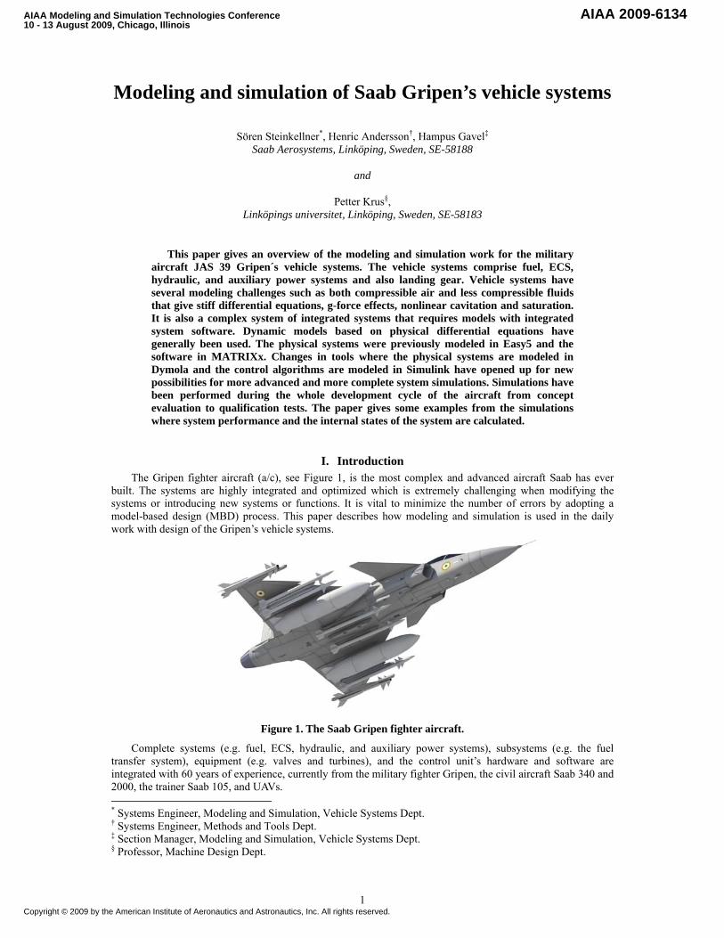
1

Modeling and simulation of Saab Gripen’s vehicle systems

Sören Steinkellner*, Henric Andersson†, Hampus Gavel‡ Saab Aerosystems, Linköping, Sweden, SE-58188

and

Petter Krus§, Linköpings universitet, Linköping, Sweden, SE-58183

This paper gives an overview of the modeling and simulation work for the military aircraft JAS 39 Gripen´s vehicle systems. The vehicle systems comprise fuel, ECS, hydraulic, and auxiliary power systems and also landing gear. Vehicle systems have several modeling challenges such as both compressible air and less compressible fluids that give stiff differential equations, g-force effects, nonlinear cavitation and saturation. It is also a complex system of integrated systems that requires models with integrated system software. Dynamic models based on physical differential equations have generally been used. The physical systems were previously modeled in Easy5 and the software in MATRIXx. Changes in tools where the physical systems are modeled in Dymola and the control algorithms are modeled in Simulink have opened up for new possibilities for more advanced and more complete system simulations. Simulations have been performed during the whole development cycle of the aircraft from concept evaluation to qualification tests. The paper gives some examples from the simulations where system performance and the internal states of the system are calculated.

I. Introduction The Gripen fighter aircraft (a/c), see Figure 1, is the most complex and advanced aircraft Saab has ever

built. The systems are highly integrated and optimized which is extremely challenging when modifying the systems or introducing new systems or functions. It is vital to minimize the number of errors by adopting a model-based design (MBD) process. This paper describes how modeling and simulation is used in the daily work with design of the Gripen’s vehicle systems.

Figure 1. The Saab Gripen fighter aircraft.

Complete systems (e.g. fuel, ECS, hydraulic, and auxiliary power systems), subsystems (e.g. the fuel transfer system), equipment (e.g. valves and turbines), and the control unit’s hardware and software are integrated with 60 years of experience, currently from the military fighter Gripen, the civil aircraft Saab 340 and 2000, the trainer Saab 105, and UAVs. * Systems Engineer, Modeling and Simulation, Vehicle Systems Dept. † Systems Engineer, Methods and Tools Dept. ‡ Section Manager, Modeling and Simulation, Vehicle Systems Dept. § Professor, Machine Design Dept.

AIAA Modeling and Simulation Technologies Conference10 - 13 August 2009, Chicago, Illinois

AIAA 2009-6134

Copyright © 2009 by the American Institute of Aeronautics and Astronautics, Inc. All rights reserved.

2

In order to achieve cost-effectiveness, modeling and simulation have been used since 1968 to develop the most complex vehicle systems. Generally speaking, modeling and simulation within vehicle systems are used today for

• Total system specification and design, e.g. functionality on the ground and in the air • Equipment specification and design • Software specification and design • Various simulators • Test rig design.

Vehicle aircraft systems are complex systems. Complex systems require complex test rigs and complex installation of the equipment in test aircraft. Simulation reduces the risk of detecting design faults late in the development work. Research has shown that early detection and correction of design faults cost 200-1,000 times less than at later stages5, see Figure 2.

Figure 2. Cost to correct design faults during the planning, development, production and customer usage

phases.

The paper begins with a background that describes modeling and simulation of a/c vehicle systems in general. This is followed by a section that describes how modeling and simulation have been implemented in the design process for development of the Gripen a/c vehicle systems. The paper ends with a summarizing paragraph containing a discussion and some conclusions.

II. Background Engineering design is a way to solve problems where a set of often unclear objectives have to be balanced without violating a set of constraints. Based on this statement, it might be said that design is essentially an optimization process, as stated by Herbert Simon18 as long ago as 1969. By employing modern modeling, simulation and optimization techniques, vast improvements can be achieved in the all parts of the design process. It is, however, recognized that for the foreseeable future there will be parts of the design process that require human or unquantifiable judgment and are thus not suitable for automation.

A great deal of research has been done in the field of engineering design and has led to different design processes and methods. Various authors present different models of the design process, such as for example Cross4, Pahl & Beitz14, Suh20, Ullman21 and Ulrich and Eppinger22. They all describe a phase-type process of different granularity with phases such as Specification, Concept Design, Preliminary Design, Detail Design, Prototype Development, Redesign, and Production (using the names along the bottom of Figure 3). One main focus of the work presented in this paper is to support the conceptual, preliminary, and detailed design phase. Ullman21 speaks of the design paradox, where very little is known about the design problem at the beginning but we have full design freedom. As time in the design process increases, knowledge about the problem is gained but the design freedom is lost due to the design decisions made during the process. To further stress the importance of the early phases of the design process, it is here that most of the cost is committed. To summarize: at the beginning of the design process of a new product, we have little knowledge of the problem, but great freedom in decision making, and the decisions we make determine much of the cost induced later in the design process. However, one would wish to be able to obtain more knowledge early on, to maintain the same high degree of design freedom and postpone the commitment of costs, as illustrated in Figure 3. The work presented in this thesis addresses, among other things, the issue of gaining knowledge early at low cost.

10: 1 Development

1:1 Planning

100:1 Production

1000:1 Usage

3

Cost Com

mitted

Cost C

ommitte

d

Freedom

Freedom

Kno

wle

dge

Know

ledge

100%

50%

0%

Today’s Design Process Future Design Process

Kno

wle

dge

Abo

ut D

esig

n D

esig

n Fr

eedo

m

Cos

t Com

mitt

ed

Con

cept

Prel

imin

ary

Des

ign

Analysisand Detail

Design

PrototypeDevelopment

Redesign Product Release

Figure 3. A paradigm shift in the design process. When knowledge about design is enhanced at an early stage, design freedom increases and cost committal is postponed. Illustration from Fabrycky7, Mavris12

and NSF13.

A. Aircraft vehicle systems In general terms, an a/c comprises three major sub-parts or sub-systems: the fuselage, the engine, and the

systems. In medium-range civil transport, the systems account for about a third of the aircraft’s empty mass as well as a third of the development and production costs17. This ratio is substantially higher (and increasing) for military aircraft.

In military a/c, the systems may then be divided into three-sub parts: the avionics, the tactical systems, and the vehicle systems. It might also be argued that the vehicle systems in a modern military a/c account for up to a third of the aircraft’s empty mass as well as a third of the development and production costs. As defined here, the vehicle systems consist of:

• fuel system • hydraulic system • environmental control systems • electrical supply system • auxiliary power system • landing gear • braking systems • escape system • de-icing system.

B. Computational design In this section some aspects of computational design are described. Computational design is a growing field

whose development is coupled to the rapid improvement of computer performance and their computational capability. There is no clear definition of the term computational design, and it is interpreted differently in different engineering domains due its broad implication. However, computational design methods are characterized by operating on computer models in different ways in order to extract information. Described here are “modeling” and “simulation”, which undoubtedly qualify as computational design activities. 1. Systems modeling

How a model may be defined in a broader sense is described by Reynolds 15 as: “A model is a representation of a system that replicates part of its form, fit, function, or a mix of the three, in order to predict how the system might perform or survive under various conditions”.

Another explanation is given by Fritzon 8, who begins by defining an experiment as extracting information about a system by exercising its inputs. A model may then be defined as something that answers questions about the system without performing experiments on the real system. Models may be mental, verbal, physical, or

4

mathematical. A simulation is then defined as an experiment performed on a model. However, this paper is limited to exploitation of mathematical models, typically those implemented in a computer environment for simulation purposes. In fact, part of this paper targets computer modeling of large physical systems specifically, which could generally be described by a mix of differential and algebraic equations.

Models easily become complex and unstructured without an appropriate tool. There are several modeling-and-simulation tools on the market today that have a graphical user interface that gives a good overview of the model. These are most often of the drag-and-drop type; this makes the modeling tool easy to use, thus minimizing the number of errors. The tools currently available include component-based tools such as Dymola, Flowmaster, Easy5, HOPSAN and AMEsim, and more equation-based tools such as Simulink and SystemBuild, among many others.

Causality is the property of cause and effect in the system and is an important condition for the choice of modeling technique and tool. For information flow or models of sensors or a CPU, the system’s inputs and outputs decide the causality. For physical systems with energy and mass flows, the causality is a question of modeling techniques/tools. In non-causal (or acausal) models, the causality is not explicitly stated, so the simulation tool has to sort the equations from the non-causal model to the simulation code. When creating a causal model of a typical energy intensive system, the modeler has to choose what is considered to be a component’s input and output, and then the bond graph modeling technique is a method that aids transformation from non-causal to causal models. Bond graph is an energy-based graphical technique for building mathematical models of dynamic systems3.

Thus, there are basically two representations, as shown in Figure 4: the signal flow/port approach using block diagrams suited for causal parts of the system and the power port approach, suitable for the non-causal parts. The chosen approach should be based on the dominating causality characteristics of the system, but is sometimes an outcome of the tool available. For instance, Simulink uses signal port and Dymola uses power port. The signal port approach clearly shows all variable couplings in the system. This is very useful for systems analysis and is therefore suitable for representing control systems and systems connected to them. However, a drawback is that the model may become complex and difficult to overview. In this case, power port modeling is more appropriate for the physical system. In power port modeling, there are bi-directional nodes that contain the transfer of several variables. Power port is more compact and closely matches the real physical connection that by nature is bi-directional. The power port technique is therefore more suitable for modeling of physical systems.

C-component,volume

Eq Eq

Pressure, p

Flow, q

Q-component,flow restrictive

p and q

Power Port(Power = p*q)

Signal Port

p and q

C/Q-component, C/Q-component,

C-component,volume

Eq Eq

Pressure, p

Flow, q

Q-component,flow restrictive

p and q

Power Port(Power = p*q)

Signal Port

p and q

C/Q-component, C/Q-component,

Figure 4. Signal flow and power port modeling.

Most simulation packages come with predefined libraries with sets of equations representing physical components. One of the major reasons for choosing a particular tool is whether a suitable component library already exists. Even so, it is not uncommon that some components may need to be tailored and added in order to simulate a specific system. When the detailed design of a library is studied more deeply, it may be found that every component is a set of equations that have to be solved. When choosing a library, it is important to know to what levels of accuracy and bandwidth the equations are valid. An example of different ways to describe a hydraulic pipe is shown in Figure 5.

5

t

qKc

Frictionq = Kc (p1-p2)0.5

p1 p2

Friction + conservation of mass + conservation of momentum + conservation of energy

temperature

Friction + Capacitance C= V/β = (q1-q2) / p (conservation of mass)

q1 q2

t

q

63%

t = C/Kc

Kc KcV

Friction +Capacitance + Inductance (L)L = (ρ*V) / A2 = (p1-p2) / q (conservation of momentum)

t

q

V m

q

tLumped Line

V m V m V m V m

t

qKc

Frictionq = Kc (p1-p2)0.5

p1 p2

qKc

Frictionq = Kc (p1-p2)0.5

p1 p2

Friction + conservation of mass + conservation of momentum + conservation of energy

temperature

Friction + conservation of mass + conservation of momentum + conservation of energy

temperature

Friction + Capacitance C= V/β = (q1-q2) / p (conservation of mass)

q1 q2

t

q

63%

t = C/Kc

Kc KcV

Friction + Capacitance C= V/β = (q1-q2) / p (conservation of mass)

q1 q2

t

q

63%

t = C/Kc

Kc KcV

Friction +Capacitance + Inductance (L)L = (ρ*V) / A2 = (p1-p2) / q (conservation of momentum)

t

q

V m

q

Friction +Capacitance + Inductance (L)L = (ρ*V) / A2 = (p1-p2) / q (conservation of momentum)

t

q

V m

q

tLumped Line

V m V m V m V m

tLumped Line

V m V m V m V m

Figure 5. Different levels of how to describe a hydraulic pipe.

2. Simulators and simulation models Simulation is an important activity for system level analysis/verification with the main objective to reduce

risk and cost. At component or sub-system level, desktop simulations in the modeling tool or in specific mid-scale-simulation software/environments add understanding and confidence to the system’s design. For a whole aircraft system, this activity is characterized as large-scale-simulation with specific prerequisites. Some definitions related to simulation are provided below:

Mid-scale simulation: The activity performed when some simulation models of aircraft subsystems, developed with different modeling techniques, are integrated into a larger model, complex enough to not be simulatable in a desktop modeling and simulation tool.

Large-scale simulation: The activity performed when several simulation models of the aircraft subsystems are integrated and specific arrangements for performance or interoperability exist. Examples of such arrangements are real-time execution, “pilot in-the-loop simulation” or “hardware in-the-loop simulation” (HILS) configurations.

Batch mode simulation: Batch analyses are performed by running the simulation in a specified set of operating points (automatically, by means of scripts). A set of scenarios are created in the same way as described for mid-scale simulations. It is also possible to introduce failures in the steady state or during the dynamic simulation. The efficiency depends on the time taken to get the stationary operating point in advance of each simulation. One way of increasing the efficiency is to calculate and save steady-state solutions to a library in advance and use these to initiate the simulation model during the batch run. For efficient batch mode simulation, a mechanism to initiate the model with predefined or previously stored states is vital.

Fault injection: Models are developed for different kinds of fault conditions that need to be simulated and analyzed, but also those for which pilot training should be carried out. What faults to model is, of course, dependent on the system concerned, but a rule of thumb is that sensors in a system are error-prone. How to model faulty conditions of a sensor is important and there are different ways to do it. A few examples are listed below:

• An intermittent fault is a fault that occurs and disappears repeatedly. Example: loose connectors. • An incipient fault is a fault that gradually develops from no fault to a larger and larger one.

Example: Slow degradation of a component. • An abrupt change is a fault that appears as a very quick change in a variable. Example: Sudden

breakdown of a component.

6

For general handling of faults in a sensor or in its connection, it is convenient to build a fault injection feature into the modeling framework. Every sensor model is then enhanced with extra output settings1. 3. Verification and validation

The general definitions of verification and validation are: • Verification. Did I build the thing right? • Validation. Did I build the right thing?

The definitions of the activities in Figure 6 according to Sargent16 are: • “Conceptual model validation is defined as determining that the theories and assumptions

underlying the conceptual model are correct and that the model representation of the problem entity is “reasonable” for the intended purpose of the model.

• Computerized model verification is defined as ensuring that the computer programming and implementation of the conceptual model is correct.

• Operational validation is defined as determining that the model’s output behavior has sufficient accuracy for the model’s intended purpose over the domain of the model’s intended applicability.”

With modeling and simulation tools, such Dymola and Simulink, the number of computer programming and implementation errors has been reduced. The activity model verification then primarily ensures that an error-free simulation language has been used, that the simulation language has been properly implemented on the computer, and the model has been programmed correctly in the simulation language16.

Problem Entity (System)

Computerized model

Conceptual model

Computerized model verification

Computer programming and implementation

Experimentation Analysis and Modeling

Operational validation Concept model validation

Figure 6. Verification and validation in the modeling process.

The activity operation validation cannot be performed in early development phases such as the concept phase due to the need for system experiment data. However, sensitivity analyses can still be done that point out model component parameters that have a strong influence on the simulation result.

III. The Gripen vehicle system development Modeling and simulation has in the past been somewhat of an activity that has been performed when

problems have been anticipated, or worse, when a problem has already occurred. Today, modeling and simulation are integrated into design process. This section describes how modeling and simulation are today a natural part of the design process and how modeling and simulation activities are exploited in the devolvement of vehicle systems for the next generation Gripen. First, the modeling and system simulation is described. This is followed by a description of the test rigs and the simulators and how the models and test facilities fit into the design process.

A. Gripen vehicle system models 1. The models

Within vehicle systems, at present, Saab AB has developed six major total system models for Gripen: • Environmental control system (ECS) • Secondary environmental control system (S-ECS) • Hydraulic supply system (HSS)

7

• Fuel system (FS) • Auxiliary power system (APESS) • Landing gear

The models are complex aircraft system models that include both the equipment and the software controlling and monitoring each system. Aircraft systems present several modeling challenges such as modeling g-force effects, mixing fuel and air in fuel systems, and flight envelope and environmental dependency of the ECS. A system model is a mix of a physical model (pumps, valves, gears, turbines, etc, i.e. machined metal or fluids that move), and software models (models of the ADA code that controls the system).

Most of the physical modeling was initially done in Easy5. The fuel system, the ECS, and the landing gear model have since been migrated into Dymola when the systems were subjected to major modifications, while the S-ECS system, which is a late addition, was modeled directly in Dymola.

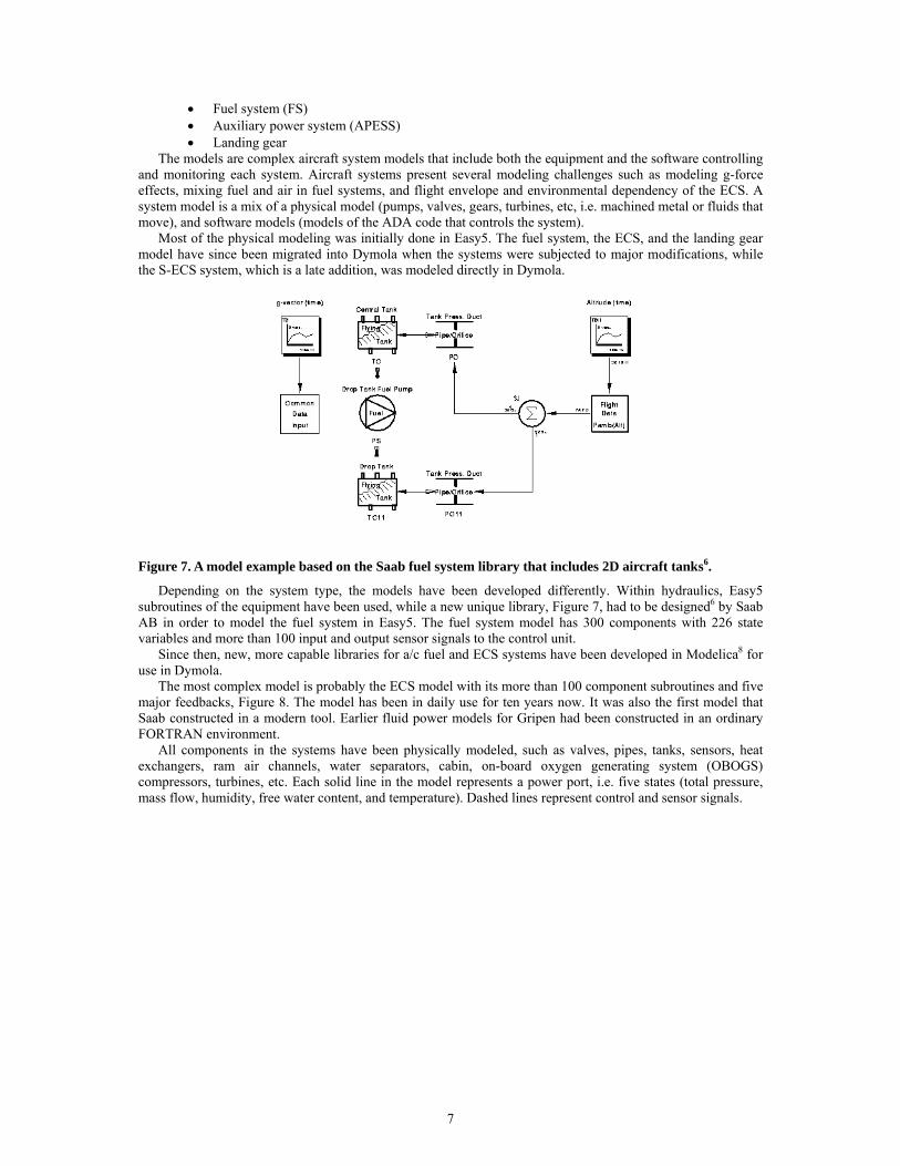
Figure 7. A model example based on the Saab fuel system library that includes 2D aircraft tanks6.

Depending on the system type, the models have been developed differently. Within hydraulics, Easy5 subroutines of the equipment have been used, while a new unique library, Figure 7, had to be designed6 by Saab AB in order to model the fuel system in Easy5. The fuel system model has 300 components with 226 state variables and more than 100 input and output sensor signals to the control unit.

Since then, new, more capable libraries for a/c fuel and ECS systems have been developed in Modelica8 for use in Dymola.

The most complex model is probably the ECS model with its more than 100 component subroutines and five major feedbacks, Figure 8. The model has been in daily use for ten years now. It was also the first model that Saab constructed in a modern tool. Earlier fluid power models for Gripen had been constructed in an ordinary FORTRAN environment.

All components in the systems have been physically modeled, such as valves, pipes, tanks, sensors, heat exchangers, ram air channels, water separators, cabin, on-board oxygen generating system (OBOGS) compressors, turbines, etc. Each solid line in the model represents a power port, i.e. five states (total pressure, mass flow, humidity, free water content, and temperature). Dashed lines represent control and sensor signals.

8

Figure 8. The ECS model of Gripen.

The system context, such as flight conditions (speed, altitude, humidity, temperature, etc.), is input to the model. So also are the interfaces to other systems where energy is transferred into the system. If necessary, the different system models are co-simulated11 or host simulated19. Dynamic models based on physical differential equations have generally been used. Black-box models have been used for some equipment of minor interest such as sensors. Tables have only been used for highly nonlinear equipment such as compressors and turbines.

Figure 9. SystemBuild model example of system software.

The control unit is represented by the system software model. The system software model is hosted as a sub-routine automatically generated from the software model, Figure 9. Integrating new code takes four hors after a minor software redesign. The control units’ hardware is partly modeled in the physical models. 2. Simulation examples

Engineers are often focused on reducing simulation times. However, experience shows that it is no less important to reduce the number of errors when complex models are to be used on a daily basis, for example:

• A system schematic’s representation of the system model on the screen with components and power ports reduces errors

• It must be user-friendly to o Change system parameters and input data – and to immediately see what has been changed o Distinguish between different plot variables o Make minor changes in the model.

T1_T(G)

NO_TANK(G)

=

=

OR

SOURCEABLE

SOURCEABLE

8

15

8

8

=4

99

BAD_TRANSF15

STATPRESS9

VOL_COR_CT1F14

TP_CMD_pp

5Select_Speed

SUPERBLOCK

Procedure 4

90

6

REG_ON

Find_TargetTARGET_p

2

9

Systems, ground supply units, and test rigs are simulated. The four major fluid power system models of Gripen can be simulated where input data such as operation conditions (e.g. altitude, speed), system conditions (e.g. defroster on or off) and equipment parameters (e.g. valve size) are changed

It is also easy to make minor changes in the model, e.g. add new components to the systems. The following is generally simulated: • Total system functionality, e.g. ECS cooling supply to avionics and cabin pressurization • Internal states such as flows, pressures, temperatures, cylinder speed, control signals, sensor signals,

etc • Function of control algorithms, e.g. if the tanks are emptied in the correct order during a mission

Figure 10. Simulated fuel tank content (right) during a flight mission (left).

Simulations have for example been used for • Evaluation of new systems’ concepts

o New system based on off-the-shelf aircraft equipment for the trainer Saab 105 o Hydraulic test set-up for dynamic testing of hydraulic connections

• System’s detailed design and redesign o Redesign of ECS from Swedish climate to world wide climate o Redesign of fuel system for air-to-air-refueling o Check of software functionality for fuel system, Figure 9. o Support for test department during fault localization, etc.

• Simulations that complete qualification tests o Simulations complement ECS tests for world wide climate when tests are conducted in test

rigs indoors or in flight tests in normal Swedish climate. o Auxiliary power system is simulated to complement tests during qualification, e.g. main

engine start on the ground and in the air, Figure 11.

9

10

Figure 11. Simulation of the auxiliary power system at engine emergency start.

B. Simulators and test rigs There are different types of simulation facilities for mid- to large-scale simulations:

• Desktop simulation tools, easy and cheap to access. • Software-based, handling qualities simulator with or without pilot in-the-loop. • Presentation and maneuvering simulator with Human-Machine-Interaction in focus. • System simulator with a large amount of target hardware and other product-equivalent equipment

present. This type of simulation is characterized as large-scale. • Test rigs including some or all of the vehicle system equipments (for a specific system e.g. fuel or

hydraulic) for system validation purpose. The list is ordered from soft to hard content.

1. Software-based simulation environments A software-based simulation model is easy to execute with a range of different user scenarios, and this can

also be done in “batch mode”, preferably distributed during “non-working hours”, to maximize the usage of the company’s computational resources. A set of scenarios is created with selected values of parameters, states, and inputs (e.g. load configuration, fuel content, speed, and altitude). Out of several simulated scenarios/maneuvers, including degraded modes, there is a selection of critical maneuvers to further verify. For each payload combination, the most severe and critical scenarios are selected for rig test or pilot-in-the-loop simulations and maybe also flight tests.

One drawback of relying on software models and simulation tools is that some aspects are difficult to cover, so a test rig with the system’s real components has to be built anyway. For example, when verifying the integrated system (hardware, software, and the environment together), aspects such as redundancy policy, timing, and performance have to be tested separately in a hardware-based rig, Figure 12. 3. Large-scale simulation

When integrating several vehicle systems, their ECUs, data buses, and other parts of the avionics system, simulation has in Saab Aerosystems’ long-term experience, proven to be an efficient method and is the most used means of system verification, e.g. before first flight. A simulation system consists of both hardware and software, but the trend is to rely more on software models of equipment that was earlier either a prototype of the production set or a simplified (hardware) equivalent. The introduction of software-based simulation systems enables more flexible and versatile usage, such as analysis through batch simulations. But new challenges in terms of for example configuration management also appear, as described below. 4. Scale-up issues

Development projects generally try to minimize the number of models of a system due to the significant administration effort that is needed and the risk of needing to handle errors following from multi-model handling. The challenge is to reuse and combine component models in a system-of-systems context, without requiring too many parameter settings and may lead to longer execution times. So, on the one hand there should be reusable and configurable (detailed) models, appropriate for both small- and large-scale usage, and on the other a sufficiently detailed, or dedicated, model that makes it easier for the user to set up and execute the simulation at a certain level.

One way to avoid several different models is to use the Multi-Level Approach reported by Kuhn10. The Multi-Level Approach allows switching between models with different levels of detail, for example:

• a simple, fast model for energy consumption design • a detailed model for fast analysis of network stability

Speed ATSSpeed Engine

Main engine restartAPU start No1

Main engine retardationWindmilling activeIgnition failure

11

• a detailed model for network quality assessment by increasing the equation complexity in the model components.

There are of course constraints to using the Multi Level Approach: for instance, the interface definitions for a model must be the same at all levels of detail (viewed as a black box).

5. Configuration handling

Challenges concerning configuration management are somewhat different and in some ways more difficult for a simulation system than for the product the simulation model represents. This is due to the possibilities to let every sub-model be configurable to represent several variants of the real component. Example: In the Gripen case, a module for calculation of weight, center of gravity and inertia has to manage data for both the one-seater and the two-seater versions as well as all possible payload configurations. Configuring is managed in several stages and there are typically some mechanisms for (variants’) configuration in simulation environment. Predefined rules exist to support variant handling and on-board configuration of the system software according to the type of equipment installed.

The need is resolved by means of switching techniques: model-time switch, compile-time switch or run-time switches. Switching during model-time creates different source code variants, and switching during compile-time creates different object codes. Run-time switching is the most flexible alternative and enables the simulation engineer to change configuration “during flight”. Which type of switching technique to use for a particular selection case depends, for example, on safety, security, and maintainability factors. For all those techniques, structured configuration tables improve the efficiency and quality of scalability in the simulation/development process.

Figure 12. The upper three photos show the rotational fuel system rig with an Air-to-Air probe. The two

lower photos show an auxiliary power system performance rig.

12

C. The model-based design process Initially, when the design of a completely new vehicle system is begun, there is conceptual design.

Conceptual design is divided into two principally different activities: concept generation and concept selection. Concept selection may then again be separated into screening the inferior concepts and identifying the superior concepts. Ultimately, one or perhaps two concept proposals are pursued into embodiment design, see Figure 13.

Time

Num

bero

f con

cept

s

Time

Screening

Scoring

Time

Num

bero

f con

cept

s

Time

Screening

Scoring

Figure 13. Concept generation and selection according to Ulrich and Eppinger22.

Computer models are a vital tool when evaluating the performance of the concept proposals. Most often, the modeling activities begin with simple stationary models of the systems, perhaps in MS Excel or equivalent9. At the end of the conceptual phase, when the number of concept proposals has decreased, more refined models are required, and dynamic models of the systems are built, at present preferably in Dymola. At this point in the evolution of the systems there is no detailed picture of the software, such as control algorithms and operating modes etc, so these are roughly modeled in the same tool. As the system goes into embodiment design, the software is modeled in a separate model with signal port technique (preferably in Simulink), which is then co-simulated or host-simulated with the physical system model.

However, most designs are actually modifications of already existing systems, if so, all the required models are present already in the early stages of the design process and relatively easy to modify for reuse. This also applies to other test facilities, such as test rigs, simulators, and test a/c, with the exception that these are not always so easy to modify

If desk top simulations do not give the complete picture, the next step is to build simulators and test rigs. The main purpose is to integrate and test the electronic control unit hardware and interface to components and systems. The amount of hardware is kept to a minimum with software-in-the-loop and desktop simulations.

Finally, flight critical functions are verified and validated with flight tests.

13

Flight test

First Loop

SecondLoop

ThirdLoop

Model of the physical system

Actual Codes/w model

M

u y

M

u y

Test rigSimulator

Figure 14. The vehicle system design process.

1. First loop, desk top simulations The first loop consists of two phases: with and without a correct software model. As mentioned earlier, a

simplified software model is implemented in the same tool as the physical system due to the later need for software details relative to the physical system development1.

In the loop without a correct software model, the physical system performance, (e.g. cooling effect, flow and maximum temperature/pressure), and dimensions, (e.g. pipe diameter and heat exchanger size), is specified for system components and to confirm the design choices in the concept phase. For some systems, the influence of the surrounding airframe on the system must also be taken into consideration, e.g. the layout of the fuel tanks.

In the loop with a correct software model, a closed loop verification (software and hardware models simulated together) can be done by co-simulation or by hosted simulation. The closed loop verification reduces the workload in simulators, rigs, and flight tests, and leads to better understanding of the impact of the software on the hardware. The major development of the software takes place in this phase. Failure mode and effect analysis (FMEA) and load analysis can also be begun late in this phase because much of the purchased system components and airframe structure design has already been frozen. In the remaining loops the major focus is on tuning, verification, and validation. 2. Second loop, simulator and rig tests The software model from the first loop is converted to actual code via autocode generation or by hand. By separating software functions according to safety criticality defined by Design Assurance Level (DAL)1 and usage of ARINC-6532 partitioning, the software functions can be safely separated so software functions of different criticality/DAL level may be hosted in the same physical computer resource. This gives major simplification of the choice of workflow, tools and verification/validation process. Examples of functions with different DAL: Critical: -Display of speed information

-Sensing and calculation of remaining fuel quantity Non-critical: -Recording of operational data for tactical evaluation Complying with the objectives according to a higher DAL is of course more costly than to a lower level and software updates of non-critical functions can be done without interfering with critical functions.

14

One purpose of the simulation activity is to verify the software algorithm and its software interface with other systems. Typical errors concern units and interfaces that are difficult to cover in loop one. A first partial validation can be done in the test rig, where the influence on the system of for example wiring and fluid dynamic, which are seldom modeled, can be analyzed. To provide some degree of flexibility in the software, the concept of Flight Test Functions (FTF) is used; system software parameters have been listed in text files so that they can be changed without re-compiling the software. An important part of the rig test activity is to feed the models with measurement data to improve the model’s accuracy. 3. Third loop, flight tests If all modified software functions are non-critical, flight tests are not considered mandatory. Some flight testing can perhaps nonetheless be conducted in parts of the flight envelope where the system model is not valid. If it is later shown in the aircraft that the software needs to be updated, this can be easily accomplished due to the separation from critical functions. If modified software functions are critical, flight tests are considered mandatory in order to secure airworthiness. The flight test should also provide the models with measurement data.

IV. Discussion and conclusions In the past, before the 1980s, new aircraft (a/c) types were developed just a couple of years apart. This was

true of both civil and military combat a/c. In those days, there was no shortage of experienced engineers in design of a new a/c. Today, 20-30 years between new a/c models is not unusual, at least not in the military industry. Although well-educated engineers are available, lack of experience in a/c specific supply systems is becoming an increasing problem for a/c system design. Therefore, methods such as the one presented in this paper are very valuable because it might be argued that a model-based approach enhances, and thus accelerates, the process of gaining experience.

References 1 Andersson, H., “Aircraft systems modeling - model based systems engineering in avionics design and aircraft

simulation.” Linköping Studies in Science and Technology, Licentiate Thesis No. 1394, ISBN 978-91-7393-692-7, Liu-Tryck Linköping 2009.

2 ARINC 653, (2006). “Avionics Application Software Standard Interface”, ARINC 653, Specification, Part 1-3, Aeronautical Radio Incorporated, Annapolis, Maryland, USA.

3 Cellier, F.E., Otter, M. and Elmqvist, H., (1995). “Bond Graph Modeling of Variable Structure Systems,” Proceedings of Second International Conference on Bond Graph Modeling and Simulation ICBGM'95, Las Vegas, USA, 1995, pages 49-55.

4 Cross, N., Engineering Design Methods, 3rd edition, John Wiley & sons, Chichester, England, 2000. 5 Backlund, G. “The Effects of Modelling Requirements in Early Phases of Buyer-Supplier Relation,”

Linköping Studies in Science and Technology, Thesis No. 812, Linköping, 2000. 6 Ellström, H., and Steinkellner, S., “Modelling of pressurized fuel systems in military aircrafts,” Proceedings

of Simulation of Onboard systems, Royal Aeronautical Society, London, 2004. 7 Fabrycky, W.J., and Blanchard, B.S., “Life-Cycle Cost and Economic Analysis,” Prentice Hall, Englewood

Cliffs, NJ, 1991. 8 Fritzson, P., Principles of Object-Oriented Modeling and Simulation with Modelica 2.2, John Wiley & sons,

USA, 2004. 9 Gavel, H., “On Aircraft Fuel Systems– Conceptual Design and System modeling,” Linköping Studies in

Science and Technology. Dissertations No. 1067, ISBN 978-91-85643-04-2, Liu-Tryck Linköping 2007. 10 Kuhn, R., ”A multi level approach for aircraft electrical systems design,” Sixth International Modelica

Conference, Vol. 1, Bielefeld, Germany, 2008, pp 95-101. 11 Larsson, J., and Krus, P., “Stability analysis of coupled simulation,” ASME International Mechanical

Engineering Congress, Vol. 1, Washington D.C., 2003, pp 861-868. 12 Mavris, D. N. and DeLaurentis, D. A., A probabilistic approach for examining aircraft concept feasibility and

viability, Aircraft Design, 2000, 3 pp.79-101. 13 National Science Foundation, “Research Opportunities in Engineering Design”. NSF Strategic Planning

Workshop Final Report (NSF Grant DMI-9521590), USA, 1996. 14 Pahl, G., and Beitz, W., Engineering Design – A Systematic Approach, Springer-Verlag, London, 1996. 15 Reynolds, M. T., Test and Evolution of Complex Systems. John Wiley & sons, 1996.

15

16 Sargent, R. G., “Verification and validation of simulation models,” 2007 Winter Simulation Conference, 2007, pp 124-37.

17 Scholtz, D., Aircraft Systems – Reliability, mass Power and Costs, European Workshop on Aircraft Design Education, 2002.

18 Simon, H., The Sciences of the Artificial, MIT Press, 1969. 19 Steinkellner, S., Andersson, H., Lind, I, and Krus, P., “Hosted simulation for heterogeneous aircraft system

development,” 26th International Congress of the Aeronautical Sciences, Anchorage, USA, ICAS2008-6.2 ST. 2008.

20 Suh, N., Axiomatic Design – Advances and Applications, Oxford University Press, 2001. 21 Ullman, D., The Mechanical Design Process, McGraw-Hill Inc. New York, 1992. 22 Ulrich, K.T., and Eppinger, S.D., Product Design and Development, 2nd Edition, McGraw-Hill, Inc., New

York, 2000.