Modeling and control of surge and rotating stall in ...
152
Transcript of Modeling and control of surge and rotating stall in ...

Modeling and Control of Surge and
Rotating Stall in Compressors
Dr.ing. thesis
Jan Tommy Gravdahl
Report 98-6-WDepartment of Engineering Cybernetics
Norwegian University of Science and TechnologyN-7034 Trondheim, Norway
1998
Abstract
This thesis contains new results in the �eld of modeling and control of rotatingstall and surge in compressors.
A close coupled valve is included in the Moore-Greitzer compression system modeland controllers for both surge and rotating stall is derived using backstepping.Disturbances, constant and time varying, are then taken into account, and non-linear controllers are derived. Stability results are given. Then, passivity is usedto derive a simple surge control law for the close coupled valve. This proportionalcontrol law is shown to stabilize the system even in the presence of time varyingdisturbances in mass ow and pressure.
A novel model for an axial compression system with non-constant compressorspeed is derived by extending the Moore-Greitzer model. Rotating stall and surgeis studied in connection with acceleration of the compressor.
Finally, a model for a centrifugal compression system with time varying compres-sor speed is derived. The variable speed compressor characteristic is derived basedon energy losses in the compressor components. Active control of surge in con-nection with varying speed is studied. Semi-global exponential stability of thecompression system with both surge and speed control is proven.
The main results of this thesis have been presented at international conferences.Parts of the thesis has also been submitted for publication in international journals.

ii Abstract
Preface and
Acknowledgments
This thesis is submitted in partial ful�llment of the requirements for the degree ofdoktor ingeni�r at the Norwegian University of Science and Technology (NTNU).The thesis is based on research done at the Department of Engineering Cybernet-ics during the period January 1995 through January 1998. It has been �nancedby a scholarship from the Research Council of Norway, under grant 107467/410.
I am grateful to my supervisor, Professor Dr.ing. Olav Egeland, for introducingme to the �eld of compressor control and control of mechanical systems in general.He has been a source of valuable advice, comments and inspiration throughout thework on this thesis and the papers on which it is based.
The sta� at the department and my colleagues are acknowledged for creating avery pleasant environment in which to do research.
I would like to thank Dr.ing. Trygve Lauvdal with whom I shared an o�ce for thepast three years. Our o�ce has been a very pleasant place to work, and we havehad numerous useful and not-so-useful discussions. Trygve is also acknowledgedfor his proofreading of this thesis.
The help of Dr.ing. Erling Aarsand Johannesen, in the form of many constructivecomments and proofreading, is greatfully acknowledged.
Finally, I would like to express my love and deepest gratitude to the three girlsin my life: To my wife G�ril for her love, continued encouragement and supportduring the work on this thesis, and to my daughters Irja and Mina for their un-conditional love.
Jan Tommy Gravdahl
March 1998, Trondheim, Norway

iv Preface and Acknowledgments
Contents
Abstract i
Preface and Acknowledgments iii
List of Figures x
1 Introduction 1
1.1 Introduction . . . . . . . . . . . . . . . . . . . . . . . . . . . . . . . 11.2 Background . . . . . . . . . . . . . . . . . . . . . . . . . . . . . . . 11.3 Stability of Compression Systems . . . . . . . . . . . . . . . . . . . 2
1.3.1 Surge . . . . . . . . . . . . . . . . . . . . . . . . . . . . . . 21.3.2 Rotating Stall . . . . . . . . . . . . . . . . . . . . . . . . . . 31.3.3 Stability Analysis . . . . . . . . . . . . . . . . . . . . . . . . 5
1.4 Modeling of Compression Systems . . . . . . . . . . . . . . . . . . 61.5 Control of Surge and Rotating Stall . . . . . . . . . . . . . . . . . 7
1.5.1 Surge/Stall Avoidance . . . . . . . . . . . . . . . . . . . . . 71.5.2 Active Surge/Stall Control . . . . . . . . . . . . . . . . . . 7
1.6 Contributions of this Thesis . . . . . . . . . . . . . . . . . . . . . . 81.7 Outline of the Thesis . . . . . . . . . . . . . . . . . . . . . . . . . . 9
2 Close Coupled Valve Control of Surge and Rotating Stall for the
Moore-Greitzer Model 11
2.1 Introduction . . . . . . . . . . . . . . . . . . . . . . . . . . . . . . . 112.2 Preliminaries . . . . . . . . . . . . . . . . . . . . . . . . . . . . . . 13
2.2.1 The Model of Moore and Greitzer . . . . . . . . . . . . . . 132.2.2 Close Coupled Valve . . . . . . . . . . . . . . . . . . . . . . 162.2.3 Equilibria . . . . . . . . . . . . . . . . . . . . . . . . . . . . 182.2.4 Change of Variables . . . . . . . . . . . . . . . . . . . . . . 192.2.5 Disturbances . . . . . . . . . . . . . . . . . . . . . . . . . . 22
2.3 Surge Control . . . . . . . . . . . . . . . . . . . . . . . . . . . . . . 242.3.1 Undisturbed Case . . . . . . . . . . . . . . . . . . . . . . . 242.3.2 Determination of �0 . . . . . . . . . . . . . . . . . . . . . . 262.3.3 Time Varying Disturbances . . . . . . . . . . . . . . . . . . 292.3.4 Adaption of Constant Disturbances . . . . . . . . . . . . . . 34
2.4 Control of Rotating Stall . . . . . . . . . . . . . . . . . . . . . . . . 382.4.1 Undisturbed Case . . . . . . . . . . . . . . . . . . . . . . . 39
vi CONTENTS
2.4.2 Disturbed Case . . . . . . . . . . . . . . . . . . . . . . . . . 442.5 Simulations . . . . . . . . . . . . . . . . . . . . . . . . . . . . . . . 45
2.5.1 Surge Control . . . . . . . . . . . . . . . . . . . . . . . . . . 462.5.2 Rotating Stall Control . . . . . . . . . . . . . . . . . . . . . 48
2.6 Conclusion . . . . . . . . . . . . . . . . . . . . . . . . . . . . . . . 50
3 Passivity Based Surge Control 51
3.1 Introduction . . . . . . . . . . . . . . . . . . . . . . . . . . . . . . . 513.1.1 Motivation . . . . . . . . . . . . . . . . . . . . . . . . . . . 513.1.2 Notation . . . . . . . . . . . . . . . . . . . . . . . . . . . . . 52
3.2 Model . . . . . . . . . . . . . . . . . . . . . . . . . . . . . . . . . . 523.3 Passivity . . . . . . . . . . . . . . . . . . . . . . . . . . . . . . . . . 53
3.3.1 Passivity of Flow Dynamics . . . . . . . . . . . . . . . . . . 533.3.2 Passivity of Pressure Dynamics . . . . . . . . . . . . . . . . 533.3.3 Control Law . . . . . . . . . . . . . . . . . . . . . . . . . . 54
3.4 Disturbances . . . . . . . . . . . . . . . . . . . . . . . . . . . . . . 563.5 Simulations . . . . . . . . . . . . . . . . . . . . . . . . . . . . . . . 573.6 Concluding Remarks . . . . . . . . . . . . . . . . . . . . . . . . . . 58
4 A Moore-Greitzer Type Model for Axial Compressors with Non-
constant Speed 61
4.1 Introduction . . . . . . . . . . . . . . . . . . . . . . . . . . . . . . . 614.2 Preliminaries . . . . . . . . . . . . . . . . . . . . . . . . . . . . . . 634.3 Modeling . . . . . . . . . . . . . . . . . . . . . . . . . . . . . . . . 64
4.3.1 Spool Dynamics . . . . . . . . . . . . . . . . . . . . . . . . 644.3.2 Compressor . . . . . . . . . . . . . . . . . . . . . . . . . . . 664.3.3 Entrance Duct and Guide Vanes . . . . . . . . . . . . . . . 674.3.4 Exit Duct and Guide Vanes . . . . . . . . . . . . . . . . . . 674.3.5 Overall Pressure Balance . . . . . . . . . . . . . . . . . . . 694.3.6 Plenum Mass Balance . . . . . . . . . . . . . . . . . . . . . 704.3.7 Galerkin Procedure . . . . . . . . . . . . . . . . . . . . . . . 714.3.8 Final Model . . . . . . . . . . . . . . . . . . . . . . . . . . . 72
4.4 Simulations . . . . . . . . . . . . . . . . . . . . . . . . . . . . . . . 744.4.1 Unstable Equilibrium, = 0:5 . . . . . . . . . . . . . . . . . 744.4.2 Stable Equilibrium = 0:65 . . . . . . . . . . . . . . . . . . 78
4.5 Concluding Remarks . . . . . . . . . . . . . . . . . . . . . . . . . . 79
5 Modelling and Control of Surge for a Centrifugal Compressor
with Non-constant Speed 81
5.1 Introduction . . . . . . . . . . . . . . . . . . . . . . . . . . . . . . . 815.2 Model . . . . . . . . . . . . . . . . . . . . . . . . . . . . . . . . . . 82
5.2.1 Impeller . . . . . . . . . . . . . . . . . . . . . . . . . . . . . 845.2.2 Di�user . . . . . . . . . . . . . . . . . . . . . . . . . . . . . 86
5.3 Energy Transfer, Compressor Torque and E�ciency . . . . . . . . 865.3.1 Ideal Energy Transfer . . . . . . . . . . . . . . . . . . . . . 865.3.2 Compressor Torque . . . . . . . . . . . . . . . . . . . . . . . 875.3.3 Incidence Losses . . . . . . . . . . . . . . . . . . . . . . . . 885.3.4 Frictional Losses . . . . . . . . . . . . . . . . . . . . . . . . 91
CONTENTS vii
5.3.5 E�ciency . . . . . . . . . . . . . . . . . . . . . . . . . . . . 925.4 Energy Transfer and Pressure Rise . . . . . . . . . . . . . . . . . . 945.5 Choking . . . . . . . . . . . . . . . . . . . . . . . . . . . . . . . . . 965.6 Dynamic Model . . . . . . . . . . . . . . . . . . . . . . . . . . . . . 975.7 Surge Control Idea . . . . . . . . . . . . . . . . . . . . . . . . . . . 985.8 Controller Design and Stability Analysis . . . . . . . . . . . . . . . 995.9 Simulations . . . . . . . . . . . . . . . . . . . . . . . . . . . . . . . 1045.10 Conclusion . . . . . . . . . . . . . . . . . . . . . . . . . . . . . . . 107
6 Conclusions 109
Bibliography 118
A Nomenclature 119
A.1 Acronyms . . . . . . . . . . . . . . . . . . . . . . . . . . . . . . . . 119A.2 Subscripts . . . . . . . . . . . . . . . . . . . . . . . . . . . . . . . . 119A.3 Superscripts . . . . . . . . . . . . . . . . . . . . . . . . . . . . . . . 119A.4 Mathematical Symbols and De�nitions . . . . . . . . . . . . . . . . 120A.5 Symbols . . . . . . . . . . . . . . . . . . . . . . . . . . . . . . . . . 121
B Some Thermodynamic and Fluid Mechanical Relations 127
B.1 Flow and Pressure Coe�cients . . . . . . . . . . . . . . . . . . . . 127B.2 Isentropic Processes . . . . . . . . . . . . . . . . . . . . . . . . . . 128B.3 Mass Balance of the Plenum . . . . . . . . . . . . . . . . . . . . . . 129B.4 Flow through a Nozzle . . . . . . . . . . . . . . . . . . . . . . . . . 130B.5 Compressor Pressure Rise . . . . . . . . . . . . . . . . . . . . . . . 131
C Including a Close Coupled Valve in the Moore-Greitzer Model 133
D Numerical Values Used in Simulations 137
E Bounds on the Controller Parameters of Theorem 2.5 139

viii CONTENTS
List of Figures
1.1 Compressor characteristic with deep surge cycle, de Jager (1995). . 3
1.2 Physical mechanism for inception of rotating stall, Emmons et.al.
(1955). . . . . . . . . . . . . . . . . . . . . . . . . . . . . . . . . . . 4
1.3 Schematic drawing of hysteresis caused by rotating stall. . . . . . . 5
2.1 Compression system. Figure taken from Moore and Greitzer (1986) 13
2.2 Cubic compressor characteristic of Moore and Greitzer (1986). The
constants W and H are known as the semi width and semi height,
respectively. . . . . . . . . . . . . . . . . . . . . . . . . . . . . . . . 16
2.3 Compression system with CCV . . . . . . . . . . . . . . . . . . . . 17
2.4 Compressor and throttle characteristics. . . . . . . . . . . . . . . . 19
2.5 Change of variables, principal drawing . . . . . . . . . . . . . . . . 20
2.6 Negative feedback interconnection of strictly passive system with pas-
sive system . . . . . . . . . . . . . . . . . . . . . . . . . . . . . . . 38
2.7 Upper plot illustrates that _V2 + _V3 < 0 for � > ��m. Lower plot
illustrates that detP > 0 for � < �choke. . . . . . . . . . . . . . . . 43
2.8 The throttle gain is set to = 0:61, and the compressor is surging.
The controllers are switched on at � = 200. . . . . . . . . . . . . . 47
2.10 Disturbance induced surge stabilized by the adaptive controller (2.122). 47
2.9 Same situation as in Figure 2.8. However, here disturbances are
taken into account. The pressure and the mass ow disturbances
are both white noise varying between �0:05. . . . . . . . . . . . . . 48
2.11 Stabilization of rotating stall . . . . . . . . . . . . . . . . . . . . . . 49
2.12 Same simulation as in Figure 2.11, superimposed on the compressor
characteristic and in-stall characteristic . . . . . . . . . . . . . . . 49
2.13 Stabilization of rotating stall with pressure disturbances . . . . . . . 50
3.1 The closed loop system �G1;G2 . . . . . . . . . . . . . . . . . . . . . 56
3.2 The closed loop system �G1;G2 with disturbances . . . . . . . . . . . 56
3.3 Comparison of closed loop response with passivity based (solid lines)
and backstepping based (dashed lines) controllers. The controllers
were switched on at � = 400. . . . . . . . . . . . . . . . . . . . . . . 58
4.1 Principal drawing of the compression system of (Moore and Greitzer
1986). The station numbers are used as subscripts in the following. 63
x LIST OF FIGURES
4.2 Simulation of the system (4.68)-(4.71). Low B leads to rotating
stall, and high B leads to surge. . . . . . . . . . . . . . . . . . . . . 764.3 Simulations result superimposed on the compression system char-
acteristics. The compressor characteristic, the in-stall characteris-
tic and the throttle characteristic are drawn with solid, dashed and
dash-dot lines respectively. . . . . . . . . . . . . . . . . . . . . . . . 764.4 The three �rst harmonics of rotating stall. The �rst harmonic J1
has the highest maximum value. This maximum value decreases with
mode number du to the e�ect of viscosity. The lower plot shows that
J2 dominates J1 during stall inception. . . . . . . . . . . . . . . . . 774.5 System response with low Ud, resulting in the compressor being stuck
in rotating stall. . . . . . . . . . . . . . . . . . . . . . . . . . . . . 774.6 Stable equilibrium with and without B-dynamics . . . . . . . . . . . 78
5.1 Compression system with CCV. . . . . . . . . . . . . . . . . . . . . 825.2 Diagrammatic sketch of a radially vaned centrifugal compressor.
Shown here with a vaned di�user. . . . . . . . . . . . . . . . . . . . 835.3 Diagrammatic sketch of centrifugal compressor �tted with a volute. 845.4 Velocity triangle at inducer. Section through inducer at radius r1 =
D1=2. . . . . . . . . . . . . . . . . . . . . . . . . . . . . . . . . . . 855.5 Velocity triangle at impeller tip. . . . . . . . . . . . . . . . . . . . . 855.6 Incidence angles at inducer. . . . . . . . . . . . . . . . . . . . . . . 895.7 Incidence angles at di�user. . . . . . . . . . . . . . . . . . . . . . . 905.8 E�ciencies for compressor with vaned (upper plot) and annular
(lower plot) di�user. . . . . . . . . . . . . . . . . . . . . . . . . . . 935.9 Energy transfer for N = 35; 000 rpm. Compressor with annular
di�user. . . . . . . . . . . . . . . . . . . . . . . . . . . . . . . . . . 955.10 Centrifugal compressor characteristic. The left plot is for an annu-
lar di�user, and the right for a vaned di�user. The dashed lines to
the right are choke lines, also known as stone walls. . . . . . . . . 965.11 Transient response of centrifugal compression system with annular
di�user. Without surge control, the compressor goes into surge,
shown with solid lines. The system response with the surge con-
troller is shown with dashed lines. . . . . . . . . . . . . . . . . . . . 1055.12 (m(t); p(t)=p01)-trajectories plotted together with the compressor char-
acteristic. N is the compressor speed in rpm. In the case of no surge
control, the surge cycle is clearly visible, but with surge control the
state converges to the intersection of the throttle and the compressor
characteristic. . . . . . . . . . . . . . . . . . . . . . . . . . . . . . . 1065.13 Transient response of centrifugal compression system with vaned dif-
fuser. Without surge control, the compressor goes into surge. This
is plotted with a solid line. The dashed lines is the system response
when the CCV surge controller is in use. . . . . . . . . . . . . . . . 107
Chapter 1
Introduction
1.1 Introduction
This thesis presents results from an investigation on nonlinear compressor controlwhere feedback is used to stabilize the compressor to the left of the surge line. Thework is motivated by the fundamental instability problem of surge and rotatingstall which limits the range of operation for compressors at low mass ows.
This instability problem has been extensively studied and industrial solutionsbased on surge avoidance are well established. These solutions are based on keep-ing the operating point to the right of the compressor surge line using a surgemargin. There is a potential for 1) increasing the e�ciency of compressors byallowing for operation closer to the surge line than what is the case in currentsystems, and 2) increasing the range of mass ows over which the compressor canoperate stably. The increase in e�ciency and mass ow range is in particularpossible with compressor designs where the design is done with such controllersin mind. This, however, raises the need for control techniques, which stabilize thecompressor also to the left of the surge line, as disturbances or set point changesmay cause crossing of the surge line. This approach is known as active surge con-trol. Active surge control is presently an area of very intense research activity, andis also the topic of this thesis.
1.2 Background
Compressors are used in a wide variety of applications. These includes turbo-jet engines used in aerospace propulsion, power generation using industrial gasturbines, turbocharging of internal combustion engines, pressurization of gas and uids in the process industry, transport of uids in pipelines and so on.
There are four general types of compressors: reciprocating, rotary, centrifugal and
2 Introduction
axial. Some authors use the term radial compressor when refering to a centrifu-gal compressor. Reciprocating and rotary compressors work by the principle ofreducing the volume of the gas, and will not be considered further in this thesis.Centrifugal and axial compressors, also known as turbocompressors or continuous ow compressors, work by the principle of accelerating the uid to a high veloc-ity and then converting this kinetic energy into potential energy, manifested byan increase in pressure, by decelerating the gas in diverging channels. In axialcompressors the deceleration takes place in the stator blade passages, and in cen-trifugal compressor it takes place in the di�user. One obvious di�erence betweenthese two types of compressors is, in axial compressors, the ow leaves the com-pressor in the axial direction, whereas, in centrifugal compressors, the ows leavesthe compressor in a direction perpendicular to the axis of the rotating shaft. Inthis thesis both types of continuous ow compressor will be studied. The litera-ture on compressors in general is vast, and a basic introduction is given by e.g.Ferguson (1963) or Cohen et al. (1996), and more advanced topics are covered bye.g. Cumpsty (1989).
The useful range of operation of turbocompressors is limited, by choking at highmass ows when sonic velocity is reached in some component, and at low mass owsby the onset of two instabilities known as surge and rotating stall. Traditionally,these instabilities have been avoided by using control systems that prevent theoperating point of the compressions system to enter the unstable regime to theleft of the surge line, that is the stability boundary. A fundamentally di�erentapproach, known as active surge/stall control, is to use feedback to stabilize thisunstable regime. This approach will be investigated in this thesis, and it will allowfor both operation in the peak e�ciency and pressure rise regions located in theneighborhood of the surge line, as well as an extension of the operating range ofthe compressor.
1.3 Stability of Compression Systems
Compression systems such as gas turbines can exhibit several types of instabil-ities: combustion instabilities, aeroelastic instabilities such as utter and �nallyaerodynamic ow instabilities, which this study is restricted to.
Two types of aerodynamic ow instabilities can be encountered in compressors.These are known as surge and rotating stall. The instabilities limits the owrange in which the compressor can operate. Surge and rotating stall also restrictthe performance (pressure rise) and e�ciency of the compressor. According tode Jager (1995) this may lead to heating of the blades and to an increase in theexit temperature of the compressor.
1.3.1 Surge
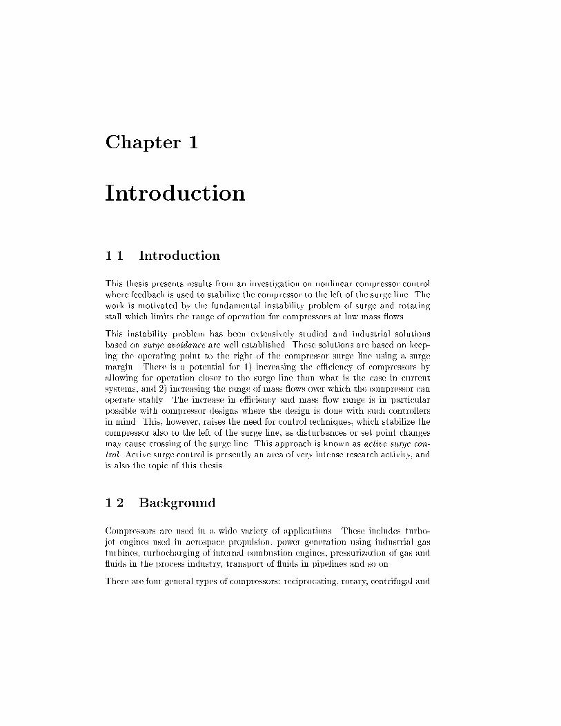
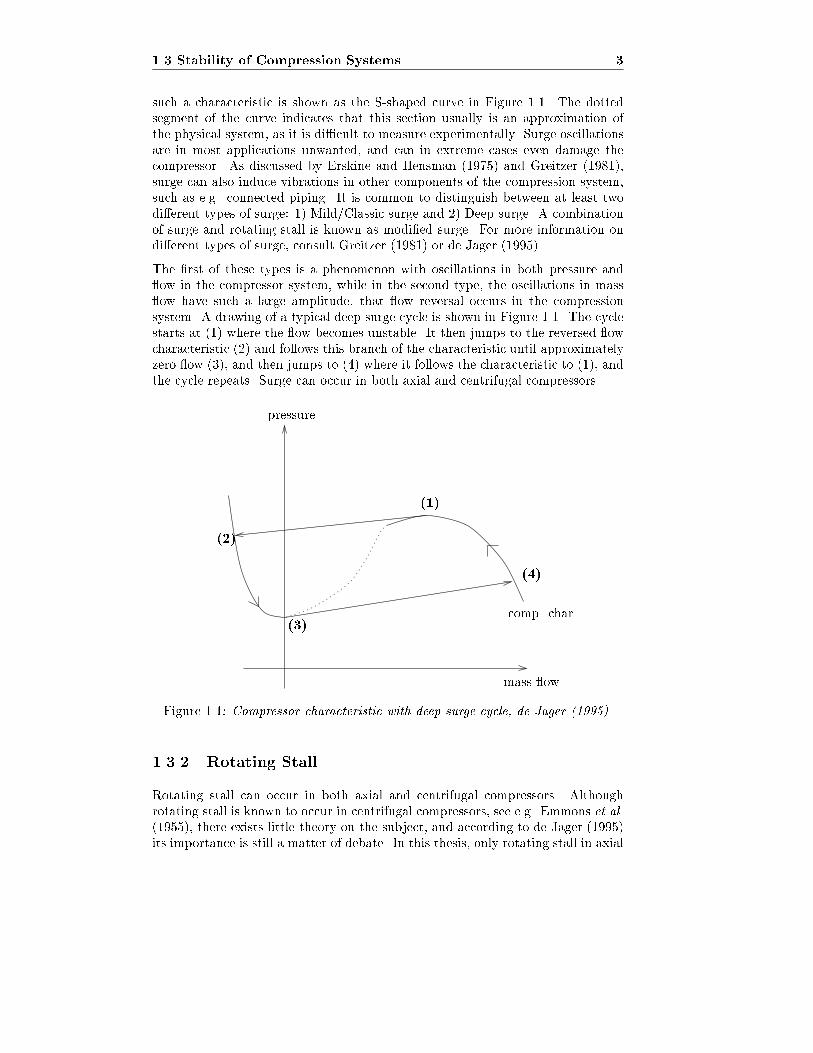
Surge is an axisymmtrical oscillation of the ow through the compressor, and ischaracterized by a limit cycle in the compressor characteristic. An example of
1.3 Stability of Compression Systems 3
such a characteristic is shown as the S-shaped curve in Figure 1.1. The dottedsegment of the curve indicates that this section usually is an approximation ofthe physical system, as it is di�cult to measure experimentally. Surge oscillationsare in most applications unwanted, and can in extreme cases even damage thecompressor. As discussed by Erskine and Hensman (1975) and Greitzer (1981),surge can also induce vibrations in other components of the compression system,such as e.g. connected piping. It is common to distinguish between at least twodi�erent types of surge: 1) Mild/Classic surge and 2) Deep surge. A combinationof surge and rotating stall is known as modi�ed surge. For more information ondi�erent types of surge, consult Greitzer (1981) or de Jager (1995).
The �rst of these types is a phenomenon with oscillations in both pressure and ow in the compressor system, while in the second type, the oscillations in mass ow have such a large amplitude, that ow reversal occurs in the compressionsystem. A drawing of a typical deep surge cycle is shown in Figure 1.1. The cyclestarts at (1) where the ow becomes unstable. It then jumps to the reversed owcharacteristic (2) and follows this branch of the characteristic until approximatelyzero ow (3), and then jumps to (4) where it follows the characteristic to (1), andthe cycle repeats. Surge can occur in both axial and centrifugal compressors.
(1)
(2)
(3)
(4)
pressure
comp. char.
mass ow
Figure 1.1: Compressor characteristic with deep surge cycle, de Jager (1995).
1.3.2 Rotating Stall
Rotating stall can occur in both axial and centrifugal compressors. Althoughrotating stall is known to occur in centrifugal compressors, see e.g. Emmons et al.(1955), there exists little theory on the subject, and according to de Jager (1995)its importance is still a matter of debate. In this thesis, only rotating stall in axial
4 Introduction
compressors will be considered, and when it is referred to rotating stall it is to beunderstood that a axial compressor is considered.
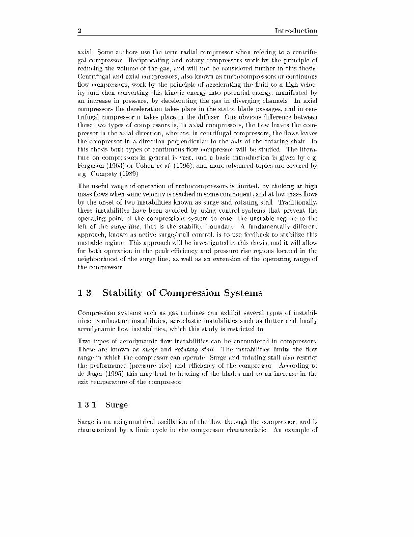
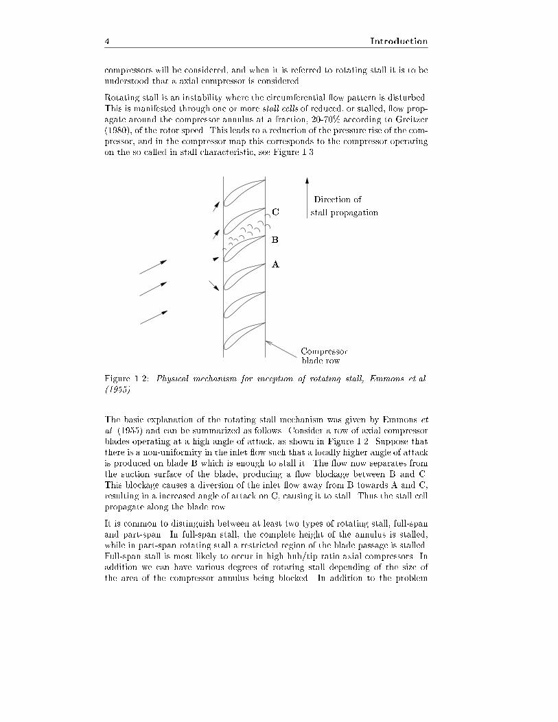
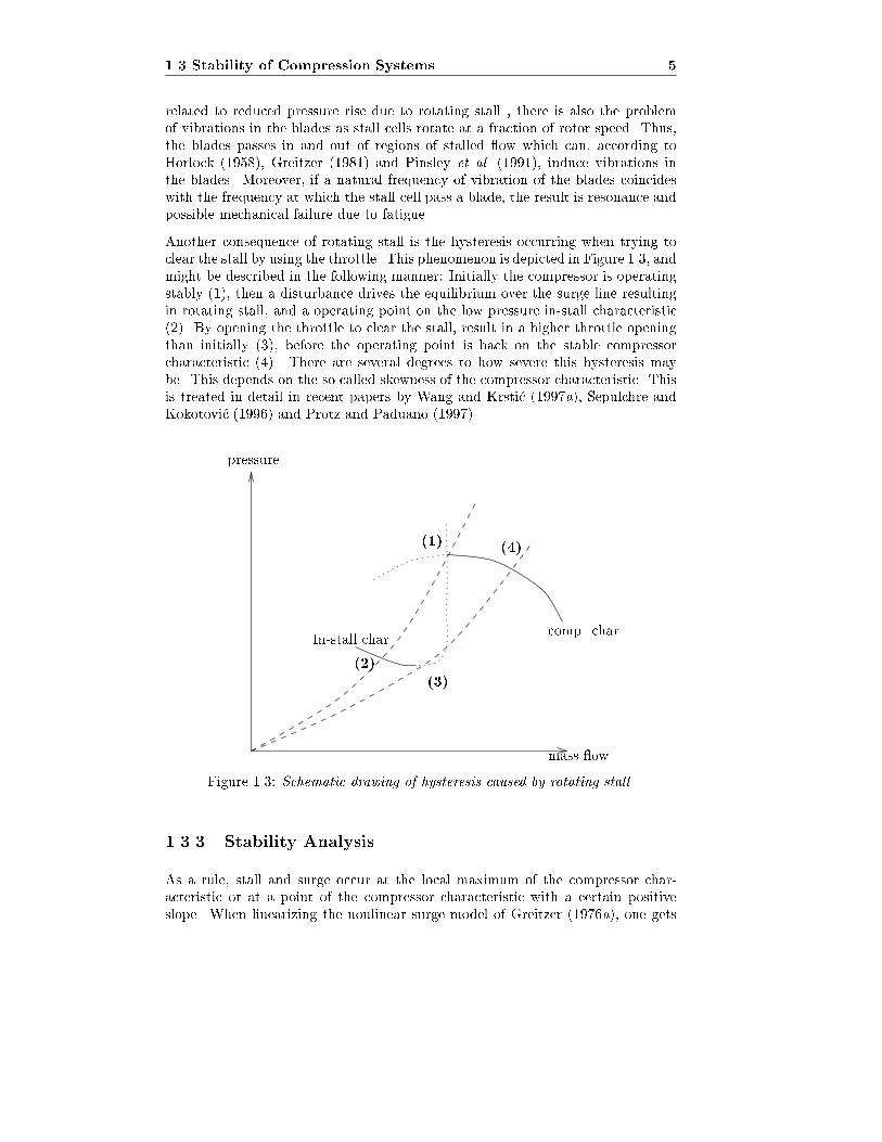
Rotating stall is an instability where the circumferential ow pattern is disturbed.This is manifested through one or more stall cells of reduced, or stalled, ow prop-agate around the compressor annulus at a fraction, 20-70% according to Greitzer(1980), of the rotor speed. This leads to a reduction of the pressure rise of the com-pressor, and in the compressor map this corresponds to the compressor operatingon the so called in-stall characteristic, see Figure 1.3.
A
B
C
Direction of
stall propagation
Compressorblade row
Figure 1.2: Physical mechanism for inception of rotating stall, Emmons et.al.
(1955).
The basic explanation of the rotating stall mechanism was given by Emmons etal. (1955) and can be summarized as follows. Consider a row of axial compressorblades operating at a high angle of attack, as shown in Figure 1.2. Suppose thatthere is a non-uniformity in the inlet ow such that a locally higher angle of attackis produced on blade B which is enough to stall it. The ow now separates fromthe suction surface of the blade, producing a ow blockage between B and C.This blockage causes a diversion of the inlet ow away from B towards A and C,resulting in a increased angle of attack on C, causing it to stall. Thus the stall cellpropagate along the blade row.
It is common to distinguish between at least two types of rotating stall, full-spanand part-span. In full-span stall, the complete height of the annulus is stalled,while in part-span rotating stall a restricted region of the blade passage is stalled.Full-span stall is most likely to occur in high hub/tip ratio axial compressors. Inaddition we can have various degrees of rotating stall depending of the size ofthe area of the compressor annulus being blocked. In addition to the problem
1.3 Stability of Compression Systems 5
related to reduced pressure rise due to rotating stall , there is also the problemof vibrations in the blades as stall cells rotate at a fraction of rotor speed. Thus,the blades passes in and out of regions of stalled ow which can, according toHorlock (1958), Greitzer (1981) and Pinsley et al. (1991), induce vibrations inthe blades. Moreover, if a natural frequency of vibration of the blades coincideswith the frequency at which the stall cell pass a blade, the result is resonance andpossible mechanical failure due to fatigue.
Another consequence of rotating stall is the hysteresis occurring when trying toclear the stall by using the throttle. This phenomenon is depicted in Figure 1.3, andmight be described in the following manner: Initially the compressor is operatingstably (1), then a disturbance drives the equilibrium over the surge line resultingin rotating stall, and a operating point on the low pressure in-stall characteristic(2). By opening the throttle to clear the stall, result in a higher throttle openingthan initially (3), before the operating point is back on the stable compressorcharacteristic (4). There are several degrees to how severe this hysteresis maybe. This depends on the so called skewness of the compressor characteristic. Thisis treated in detail in recent papers by Wang and Krsti�c (1997a), Sepulchre andKokotovi�c (1996) and Protz and Paduano (1997).
(1)
(2)
(3)
(4)
pressure
In-stall char.comp. char.
mass ow
Figure 1.3: Schematic drawing of hysteresis caused by rotating stall.
1.3.3 Stability Analysis
As a rule, stall and surge occur at the local maximum of the compressor char-acteristic or at a point of the compressor characteristic with a certain positiveslope. When linearizing the nonlinear surge model of Greitzer (1976a), one gets
6 Introduction
a model similar to that of a damped linear oscillator. This surge model was alsostudied by Stenning (1980). Calculating the eigenvalues of the oscillator system,as done by Willems (1996) , reveals that the stability boundary is set by a relationbetween the slope of the compressor characteristic, the slope of the load line, andthe Greitzer B-parameter. The surge point will be located some small distance tothe left of the peak. According to Cumpsty (1989), the peak of the compressorcharacteristic provides a convenient working approximation for the surge point.The same conclusion is drawn by Stenning (1980), where it is also pointed outthat rotating stall occurs at the peak of the compressor characteristic.
Another approach frequently used to investigate stability of compression systemsis bifurcation analysis. For studies on this topic, consult McCaughan (1989), Liawand Abed (1992) or Abed et al. (1993).
1.4 Modeling of Compression Systems
Low order models for surge in compression systems, both axial and centrifugal,have been proposed by many authors. A classical reference is Emmons et al.
(1955). In the following, a compression system will refer to a system consisting ofa compressor pressurizing incompressible uid, which is discharged into a plenumvolume which discharges via a throttle valve.
The compression system model of Greitzer (1976a) has been widely used for surgecontrol design. It was derived for axial compression systems, but Hansen et al.
(1981) showed that it is also applicable to centrifugal compressors. The model hastwo states, normalized mass ow and normalized pressure, and the compressor istreated as an actuator disc, with a third order polynomial ow/pressure rise char-acteristic. Other assumptions of this model are: one dimensional incompressible ow in the ducts, isentropic compression process in the plenum and no spatialvariations of pressure in the plenum. Extensive experiments by Greitzer (1976b)and Hansen et al. (1981) con�rm that although it is of low order compared to thecomplex phenomenon it models, the model is capable of describing both the qual-itative and quantitative aspects of surge. The model was extended for centrifugalcompressors with varying rotor speed by Fink et al. (1992). Many other models ofcompression systems have been presented in the literature, for an overview consultWillems (1996).
Based on the work of Moore (1984b), the Moore-Greitzer model was derived inMoore and Greitzer (1986). In developing this model, some of the assumptionsmade were: Large hub/tip ratio, irrotational and inviscid ow in the inlet duct,incompressible compressor mass ow, short throttle duct, small pressure rise com-pared to ambient conditions and constant rotor speed. A Galerkin procedure wasused to approximate the PDEs describing the system dynamics by three ODEs.This three state model is capable of describing both surge and rotating stall, thethird state being the stall amplitude. Many authors have extended and modi-�ed the model. Inclusion of higher order harmonics was studied by Mansoux et
al. (1994), and other types of compressor characteristics was used by Wang and
1.5 Control of Surge and Rotating Stall 7
Krsti�c (1997a).
An alternative model of rotating stall was presented by Paduano et al. (1995),where rotating stall was described as a traveling wave, and spatial Fourier analysiswas used. Other models that are capable of demonstrating rotating stall arethose of Eveker and Nett (1991) and Badmus et al. (1995), but these models donot include the stall amplitude as a state, but the presence of rotating stall ismanifested as a pressure drop.
1.5 Control of Surge and Rotating Stall
1.5.1 Surge/Stall Avoidance
As mentioned above, the state of art in control of compressors was until about adecade ago, the method of surge avoidance, which is usually an open loop strategyaccording to de Jager (1995). The compressor is prevented from operating in aregion near and beyond the surge line. This is achieved by e.g. recirculation of the ow or blowing o� ow through a bleed valve. As the compressor characteristicand thus the surge line may be poorly known, it will often be necessary to havea fairly conservative surge margin between the surge line and the surge avoidanceline. The compressor is then not allowed to operate between these two lines in thecompressor map. Accounting for possible disturbances also a�ects the size of thesurge margin.
The drawbacks of surge avoidance schemes are several: (1) Recycling and bleedingof compressed ow lower the e�ciency of the system, (2) maximum e�ciencyand pressure rise may not be achievable at all, as they usually are achieved formass ows close to the surge line and (3) the surge margin limits the transientperformance of the compressor as acceleration of the machine tends to drive thestate of the system towards the surge line.
An alternative to surge avoidance is surge detection and avoidance. Using thisstrategy, the drawbacks of the surge margin can be avoided by the activation ofthe controller if the onset of instabilities is detected. De Jager (1995) concludesthat the main disadvantages of this strategy are problems associated with thedetection of the instability onset and the necessity of large control forced andfast-acting control systems.
1.5.2 Active Surge/Stall Control
The approach of active surge/stall control aims at overcoming the drawbacks ofsurge avoidance, by stabilizing some part of the unstable area in the compressormap using feedback. This approach was introduced in the control literature byEpstein et al. (1989). In the last decade, the literature on feedback stabilization ofcompression systems has become extensive. This is partly due to the introduction,and success, of the Moore-Greitzer model.
8 Introduction
In the literature on developments in the �eld of jet engines for aircraft propulsion,active stall/surge control is often said to become an important part of futureengines. For details see e.g. Covert (1995), Ru�es (1996) or DeLaat et al. (1996).The term \smart engines" is often used when refering to these engines. Brownet al. (1997) reports of successfull in- ight experiments on a F-15 aircraft withactive stall control on one engine. Experimental results on laboratory engines arereported by Paduano et al. (1993), Ffowcs Williams et al. (1993), Hynes et al.
(1994) and Behnken and Murray (1997).
Among several possible actuators for stabilizing compression systems, the throttlevalve as studied by Krsti�c et al. (1995b) and Badmus et al. (1996), or bleed valves asstudied by Eveker and Nett (1991) or Murray (1997) has been the most commonlyused, at least in the control literature. Other possibilities are variable inlet guidevanes as in Paduano et al. (1993), loudspeaker as in Ffowcs Williams and Huang(1989), tailored structures as in Gysling et al. (1991), recirculation as in Balchenand Mumm�e (1988), movable wall as in Epstein et al. (1989) or air injection as inDay (1993) and Behnken and Murray (1997). However, the use of a close-coupledvalve (hereafter named CCV) was claimed by Simon et al. (1993) and van de Wal etal. (1997) to be among the most promising actuators for compressor surge control.
The methods used for designing surge and stall controllers vary. Linearization andcomplex-valued proportional control was used by Epstein et al. (1989), bifurcationtheory by Liaw and Abed (1996), feedback linearization by Badmus et al. (1996),Lyapunov methods by Simon and Valavani (1991), backstepping by Krsti�c et al.(1995b) and H1 by van de Wal et al. (1997) and Weigl and Paduano (1997). Inthis thesis, backstepping, which is Lyapunov based, and passivity will be used.
Another important aspect of active surge and stall control is the disturbance rejec-tion capabilities and robustness of the proposed controllers. Greitzer and Moore(1986) recognized that research is needed on modeling of disturbances in compres-sion systems. The reason for this being that disturbances may initiate surge orrotating stall. Surge controllers with disturbance rejection was presented by Si-mon and Valavani (1991) and stall/surge controllers by Haddad et al. (1997), andstall/surge controllers for compressors with uncertain compressor characteristicwas studied by Leonessa et al. (1997b).
1.6 Contributions of this Thesis
The contributions of this thesis can be summarized as follows:
� Close coupled valve control of the Moore-Greitzer model: Con-trollers for a close coupled valve in a Moore-Greitzer type compression sys-tem have been derived. The controllers allow for stabilization of rotating stalland surge to the left of the compressors surge line. The e�ect of constant andtime varying disturbances has also been studied, and controllers have beenderived that ensures avoidance of stall and surge when these disturbances arepresent in the compression system. The theory used is backstepping. This
1.7 Outline of the Thesis 9
work has been published in Gravdahl and Egeland (1997c) and Gravdahland Egeland (1997d), and is also reported in Gravdahl and Egeland (1998a).
� Passivity based surge control: A surge control law has been derived forthe Greitzer model using passivity and a input-output model. The resultingcontroller is very simple and is shown to render the system L2-stable alsowhen disturbances are taken into account. Parts of this work has beenpublished in Gravdahl and Egeland (1997f) and submitted in Gravdahl andEgeland (1998c).
� Post stall modeling of axial compression systems with non-constant
speed: An extension of the Moore-Greitzer model has been derived to takenon-constant compressor speed into account. This new model also includeshigher harmonics of rotating stall. The work is published in Gravdahl andEgeland (1997a) and is also reported in Gravdahl and Egeland (1997e)
� Centrifugal compressor modeling and control: A speed dependentcompressor characteristic for a centrifugal compressor has been derived bythe use of energy transfer and losses in the compressor components. Thischaracteristic has been used in a dynamic model of a compression systemwith time varying compressor speed, to derive controllers that simultaneouslysuppress surge and ensures that desired speed is reached. This work hasbeen published in Gravdahl and Egeland (1997g) and Gravdahl and Egeland(1998b), and is also under consideration for publication in Gravdahl andEgeland (1997b).
The results reported of in this Thesis is also accepted for publication in Gravdahl(1998).
1.7 Outline of the Thesis
The outline of this thesis is as follows
� Chapter 2: The Moore-Greitzer model and the actuator used in this thesesfor surge/stall control, the close coupled valve, are presented. Using back-stepping, various controllers are derived. These includes controllers for surgewith time varying and constant disturbances (in the later case an adaptivecontroller is derived) and controllers for rotating stall with time varying dis-turbances. Stability results are given for each controller.
� Chapter 3: Passivity is used to derive a surge control law. The controlleris shown to maintain certain stability properties even if disturbances areconsidered.
� Chapter 4: An extension of the familiar Moore-Greitzer model is presented.This model includes Greitzer's B-parameters as a state, which is a conse-quence of relaxing the assumption of constant compressor speed.
10 Introduction
� Chapter 5: Here a novel model for a compression system with a variablespeed centrifugal compressor is derived. Using Lyapunov theory, controllersare derived that ensures suppression of surge and regulation of speed. Theclosed loop system is shown to be semi globally exponentially stable.
� Chapter 6: Conclusions
� Finally, references and �ve appendices are given at the end of the thesis.A nomenclature is given in Appendix A.
Chapter 2
Close Coupled Valve Control
of Surge and Rotating Stall
for the Moore-Greitzer
Model
2.1 Introduction
In this chapter controllers for surge and rotating stall using a CCV is derived.Several possible actuators exists for stabilizing compression systems. Krsti�c et al.(1995b), Badmus et al. (1996) and others suggest using a variable throttle valve,Eveker and Nett (1991), Murray (1997) and others use bleed valves. These twoactuators have been the most commonly used, at least in the control literature.However, there are many other possibilities: Paduano et al. (1993) use variableinlet guide vanes, a loudspeaker is used by Ffowcs Williams and Huang (1989),tailored structures in Gysling et al. (1991), recirculation is studied by Balchen andMumm�e (1988), a movable wall in Epstein et al. (1989) and �nally Day (1993) andBehnken and Murray (1997) employ air injection. However Simon et al. (1993)claimed that the use of a close-coupled valve (hereafter named CCV) is among themost promising actuators for active surge control.
The use of a CCV for control of compressor surge was studied by Dussourd et al.
(1976), Greitzer (1981), Pinsley et al. (1991), Simon and Valavani (1991), Simon etal. (1993) and Jungowski et al. (1996). Experimental results of compressor surgecontrol using a CCV was reported by Erskine and Hensman (1975) and Dussourdet al. (1977). Simon (1993) and Simon et al. (1993) compared, using linear theory,this strategy to a number of other possible methods of actuation and sensing. Theconclusion was that the most promising method of surge control is to actuate thesystem with feedback from the mass ow measurement to a CCV or an injector. In
12
Close Coupled Valve Control of Surge and Rotating Stall for the
Moore-Greitzer Model
line with this conclusion are the recent results of van de Wal and Willems (1996)and van de Wal et al. (1997), where nonlinear controllers were derived based onH1 performance speci�cations.
Dussourd et al. (1976), Greitzer and Griswold (1976), Dussourd et al. (1977),Greitzer (1977) and Greitzer (1981) conclude that downstream components incompression systems have an impact on the onset of rotating stall. Dussourd et
al. (1977) used a CCV to achieve a signi�cant extension of ow range, and it wasconcluded that the CCV also a�ected the onset of rotating stall as well as surge.Osborn and Wagner (1970) report of experiments where rotating stall in an axial- ow fan rotor was suppressed, at the cost of a drop in e�ciency, by a movable\door" close coupled downstream of the rotor. The door had a similar geometryto that of a axisymmetric nozzle, and the experimental setup simulated a turbofanengine. Greitzer (1977) found that a downstream nozzle shifted the point of onsetof rotating stall to lower mass ows, however the e�ect was strongest for singlecell, full span stall. The Moore-Greitzer model, which is going to be used in thischapter, assumes a high hub to tip ratio compressor, which is likely to exhibit fullspan stall. Moreover, Greitzer (1977) found that the stabilizing e�ect of the nozzlefalls rapidly with increasing distance between compressor and nozzle, and therebyemphasizing the importance of close coupling between compressor and actuator,a point also made by Hendricks and Gysling (1994). Based on this, the CCV willin this thesis not only be used as an actuator to stabilize surge, but also rotatingstall.
Simon and Valavani (1991) studied the stability of a compressor with CCV con-trol by using a Lyapunov function termed the incremental energy. The controllaw developed by Simon and Valavani (1991) requires knowledge of the compres-sor characteristic, and additional adjustments to the controller dictated by theLyapunov analysis is performed in order to avoid a discontinuous controller.
Here we will use the backstepping methodology of Krsti�c et al. (1995a) to derivea control law for a CCV which gives a GAS equilibrium beyond the original surgeline. Simon and Valavani (1991) studied the e�ect on stability of disturbances inpressure rise. This will be considered also here, and in addition we will also considerdisturbances in the plenum out ow. In the case of only pressure disturbances, wewill derive a controller that only requires knowledge of an upper bound on the slopeof the compressor characteristic in order to guarantee stability. Discontinuity isnot a problem with this controller. Under mild assumptions on the disturbances,global uniform boundedness and convergence will be proven in the presence ofboth pressure and mass ow disturbances. Constant disturbances or o�sets willalso be considered.
Krsti�c and Kokotovi�c (1995) and Krsti�c et al. (1995b) used backstepping to designanti surge and anti stall controllers. The actuator used was a variable throttle.Here, we use the pressure drop across the CCV as the control variable. Pinsleyet al. (1991) pointed out that in compression systems with large B-parameter (tobe de�ned), the use of a CCV is expected to be more e�ective than the use of thethrottle in control of surge. In this case the ow through the throttle is less coupledwith the ow through the compressor than is the case when the B-parameter is
2.2 Preliminaries 13
small. Pinsley et al. (1991), Krsti�c and Kokotovi�c (1995) and Krsti�c et al. (1995b)use feedback from mass ow and pressure. As will be shown, the application of thebackstepping procedure to CCV surge and stall control, in the case of no mass owdisturbances, results in a control law which uses feedback from mass ow only.
As opposed to throttle control, CCV control modi�es the compressor character-istic. This allows for, at the cost of a pressure loss over the valve, recovery fromrotating stall beyond the surge line. Although the pressure rise achieved in thecompression system with a steady pressure drop across the CCV is comparablewith the pressure rise achieved when the machine is in rotating stall, the CCVapproach is to prefer as the possibility for blade vibration and high temperaturesis avoided.
2.2 Preliminaries
2.2.1 The Model of Moore and Greitzer
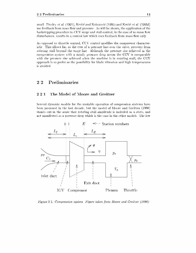
Several dynamic models for the unstable operation of compression systems havebeen proposed in the last decade, but the model of Moore and Greitzer (1986)stands out in the sense that rotating stall amplitude is included as a state, andnot manifested as a pressure drop which is the case in the other models. The low
HHHHH
�����
AAA���
Station numbersE10
LI
Lc
LE
�
�
pTCx
ps
pT
Vp
ThrottlePlenum
Exit duct
CompressorIGV
Inlet duct
Figure 2.1: Compression system. Figure taken from Moore and Greitzer (1986)
14
Close Coupled Valve Control of Surge and Rotating Stall for the
Moore-Greitzer Model
order1 model of Moore and Greitzer (1986) captures the post stall transients ofa low speed axial compressor-plenum-throttle (see Figure 2.1) system. The mainassumptions made by Moore and Greitzer (1986) in deriving the model are: largehub-to-tip ratio so that a two-dimensional description seems reasonable, incom-pressible compressor mass ow, compressible ow in the plenum, spatially uniformplenum pressure and short throttle duct. The three di�erential equations of themodel arises from a Galerkin approximation of the local momentum balance, theannulus-averaged momentum balance and the mass balance of the plenum. Acubic compressor characteristic is assumed. The model is given by:
_ =W=H
4B2
��
W� 1
W�T ()
�H
lc
_� =H
lc
� � c0
H� 1
2
��
W� 1
�3+ 1 +
3
2
��
W� 1
��1� J
2
�!(2.1)
_J = J
1�
��
W� 1
�2� J
4
!%
where
� � is the annulus averagedmass ow coe�cient (axial velocity divided by com-
pressor speed), where the annulus average is de�ned as 12�
R 2�0
�(�; �)d�4=
�(�), and �(�; �) is the local mass ow coe�cient,
� is the non dimensional plenum pressure or pressure coe�cient (pressuredivided by density and the square of compressor speed),
� J is the squared amplitude of rotating stall amplitude
� �T () is the throttle mass ow coe�cient and
� lc is the e�ective ow-passage nondimensional length of the compressor andducts de�ned as
lc4= lI +
1
a+ lE ; (2.2)
where the positive constant a is the reciprocal time-lag parameter of theblade passage,
For a discussion of the employed nondimensionalization, consult Appendix B. Theconstant B > 0 is Greitzer's B-parameter de�ned by Greitzer (1976a) as
B4=
U
2as
rVp
AcLc; (2.3)
where U is the constant compressor tangential speed (in m/s) at mean diameter,as is the speed of sound, Vp is the plenum volume, Ac is the ow area and Lc is
1\Low order" refers to the simplicity of the model, three states, compared to the complex
uid dynamic system it models
2.2 Preliminaries 15
the length of ducts and compressor. The constant % > 0 is de�ned as
% =3aH
(1 +ma)W; (2.4)
where m is the compressor-duct ow parameter, H is the semi-height of the com-pressor characteristic and W is the semi-width of the compressor characteristic.The time variable � used throughout this chapter is also nondimensional, and isde�ned as
�4= Ut=R (2.5)
where t is the actual time and R is the mean compressor radius. The notation _�is to be understood as the derivative of � with respect to �, that is _� = d�
d�.
Relaxing the constant speed assumption is important for studying e�ects of setpoint changes, acceleration, deceleration, etc. A model taking variable speed intoaccount will be developed in Chapter 4, but will not be considered further here.
In the case of pure surge, that is when J � 0, the model reduces to that of Greitzer(1976a):
_� =1
lc(c(�)�) (2.6)
_ =1
4B2lc(���T ()):
In Greitzer (1976a), the model was written
_� = B(c(�)�)
_ =1
B(���T ()):
The discrepancy in the constants is due to Greitzer (1976a) de�ning nondimen-sional time as � = t!H where !H is the Helmholtz frequency. Here, nondimensionaltime is de�ned according to (2.5), as was also done by Moore and Greitzer (1986).The model (2.6) was derived for axial compression systems, but it was demon-strated by Hansen et al. (1981) that the model also is applicable to centrifugalsystems.
The pressure rise of the compressor is a nonlinear function of the mass ow. Thisfunction, c(�), is known as the compressor characteristic. Di�erent expressionsfor this characteristic have been used, but one that has found widespread accep-tance in the control literature is the cubic characteristic of Moore and Greitzer(1986):
c(�) = c0 +H
1 +
3
2
��
W� 1
�� 1
2
��
W� 1
�3!; (2.7)
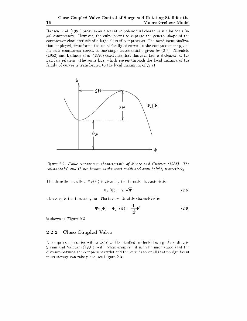
where the constant c0 > 0 is the shut-o� value of the compressor character-istic. The cubic characteristic with the parameters c0, W and H is shown inFigure 2.2. Mansoux et al. (1994), Sepulchre and Kokotovi�c (1996) and Wang andKrsti�c (1997a) suggest other compressor characteristics for axial compressors, and
16
Close Coupled Valve Control of Surge and Rotating Stall for the
Moore-Greitzer Model
Hansen et al. (1981) presents an alternative polynomial characteristic for centrifu-gal compressors. However, the cubic seems to capture the general shape of thecompressor characteristic of a large class of compressors. The nondimensionaliza-tion employed, transforms the usual family of curves in the compressor map, onefor each compressor speed, to one single characteristic given by (2.7). Nisenfeld(1982) and Badmus et al. (1996) concludes that this is in fact a statement of theFan law relation. The surge line, which passes through the local maxima of thefamily of curves is transformed to the local maximum of (2.7).
�
c(�)2H
2W
c0
Figure 2.2: Cubic compressor characteristic of Moore and Greitzer (1986). The
constants W and H are known as the semi width and semi height, respectively.
The throttle mass ow �T () is given by the throttle characteristic
�T () = Tp (2.8)
where T is the throttle gain. The inverse throttle characteristic
T (�) = ��1T(�) =
1
2T
�2 (2.9)
is shown in Figure 2.5.
2.2.2 Close Coupled Valve
A compressor in series with a CCV will be studied in the following. According toSimon and Valavani (1991), with \close-coupled" it is to be understood that thedistance between the compressor outlet and the valve is so small that no signi�cantmass storage can take place, see Figure 2.3.
2.2 Preliminaries 17
������
PPPP
PP
��@@
��@@
Compressor
CCV
c(�)
v(�)
Throttle�T ()
Plenum
�
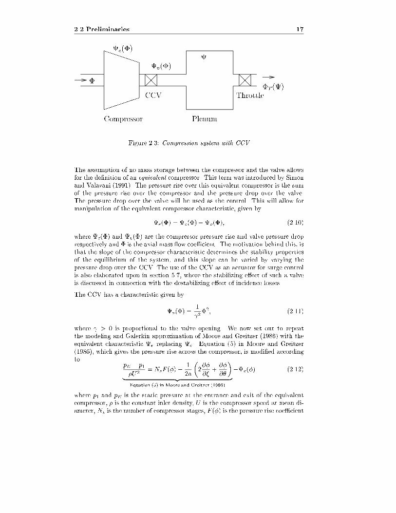
Figure 2.3: Compression system with CCV
The assumption of no mass storage between the compressor and the valve allowsfor the de�nition of an equivalent compressor. This term was introduced by Simonand Valavani (1991). The pressure rise over this equivalent compressor is the sumof the pressure rise over the compressor and the pressure drop over the valve.The pressure drop over the valve will be used as the control. This will allow formanipulation of the equivalent compressor characteristic, given by
e(�) = c(�)�v(�); (2.10)
where c(�) and v(�) are the compressor pressure rise and valve pressure droprespectively and � is the axial mass ow coe�cient. The motivation behind this, isthat the slope of the compressor characteristic determines the stability propertiesof the equilibrium of the system, and this slope can be varied by varying thepressure drop over the CCV. The use of the CCV as an actuator for surge controlis also elaborated upon in section 5.7, where the stabilizing e�ect of such a valveis discussed in connection with the destabilizing e�ect of incidence losses.
The CCV has a characteristic given by
v(�) =1
2�2; (2.11)
where > 0 is proportional to the valve opening. We now set out to repeatthe modeling and Galerkin approximation of Moore and Greitzer (1986) with theequivalent characteristic e replacing c. Equation (5) in Moore and Greitzer(1986), which gives the pressure rise across the compressor, is modi�ed accordingto
pE � p1
�U2= NsF (�)� 1
2a
�2@�
@�+@�
@�
�| {z }
Equation (5) in Moore and Greitzer (1986)
�v(�) (2.12)
where p1 and pE is the static pressure at the entrance and exit of the equivalentcompressor, � is the constant inlet density, U is the compressor speed at mean di-ameter, Ns is the number of compressor stages, F (�) is the pressure rise coe�cient
18
Close Coupled Valve Control of Surge and Rotating Stall for the
Moore-Greitzer Model
in the blade passage, and � is the angular coordinate around the wheel. Equation(2.12) now gives the pressure rise over the equivalent compressor.
Using (2.12) as a starting point and following the derivation of Moore and Greitzer(1986), the following model is found2:
_ =W=H
4B2
��
W� 1
W�T ()
�H
lc
_� =H
lc
� � c0
H� 1
2
��
W� 1
�3+ 1
+3
2
��
W� 1
��1� J
2
�� 1
2
�W 2J
2H+�2
H
�!(2.13)
_J = J
1�
��
W� 1
�2� J
4� 1
24W�
3H
!%;
which will be used in design of stall/surge controllers in this chapter. In the simplercase of pure surge, J is set to zero, and we are left with the model
_ =1
4B2lc(���T ( )) (2.14)
_� =1
lc(c(�)�v(�)�)
which will used in the study of surge control.
2.2.3 Equilibria
The compressor is in equilibrium when _� = _ = _J = 0. If J(0) = 0 then J � 0and the equilibrium values �0 and 0 are given by the intersection of e(�) andthe throttle characteristic. If J(0) > 0, and the throttle characteristic crossese to the left of the local maximum, the compressor may3 enter rotating stalland the equilibrium values �0 and 0 are given by the intersection of the throttlecharacteristic and the stall characteristic es(�) which is found by analyzing the_J-equation of (2.13). It is seen that _J = 0 is satis�ed for J = 0 or
J = Je = 4
1�
��
W� 1
�2� 1
24W�
3H
!: (2.15)
Inserting (2.15) in the _�-equation of (2.13) and setting _� = 0 gives the expressionfor es(�) :
es(�) = s(�) +5
Hv(�)� 8W
H 2
�1� W 2
3H2 2
��; (2.16)
2The complete derivation is shown in Appendix C.3This depends on the numerical value of B. Greitzer and Moore (1986) showed that small B
gives rotating stall, and large B gives surge.
2.2 Preliminaries 19
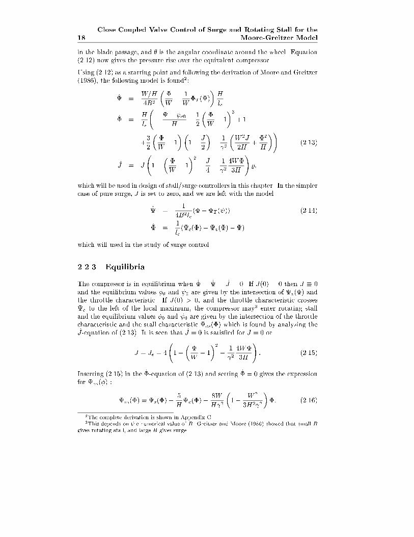
where
s(�) = c0 +H
1� 3
2
��
W� 1
�+5
2
��
W� 1
�3!(2.17)
is the stall characteristic found when the CCV is not present. In Figure 2.4 thevarious characteristics are shown. As can be seen, the throttle line intersects c ina point of positive slope, that is in the unstable area of the compressor map, andthe compressor would go into rotating stall or surge. By introducing the CCV, thethrottle line crosses the equivalent characteristic e in an area of negative slope.This new equilibrium is thus stable.
−0.2 −0.1 0 0.1 0.2 0.3 0.4 0.5 0.6 0.7 0.80
0.1
0.2
0.3
0.4
0.5
0.6
0.7
0.8
�
c(�)
e(�)
v(�)
s(�)
es(�)
��1(�)
Figure 2.4: Compressor and throttle characteristics.
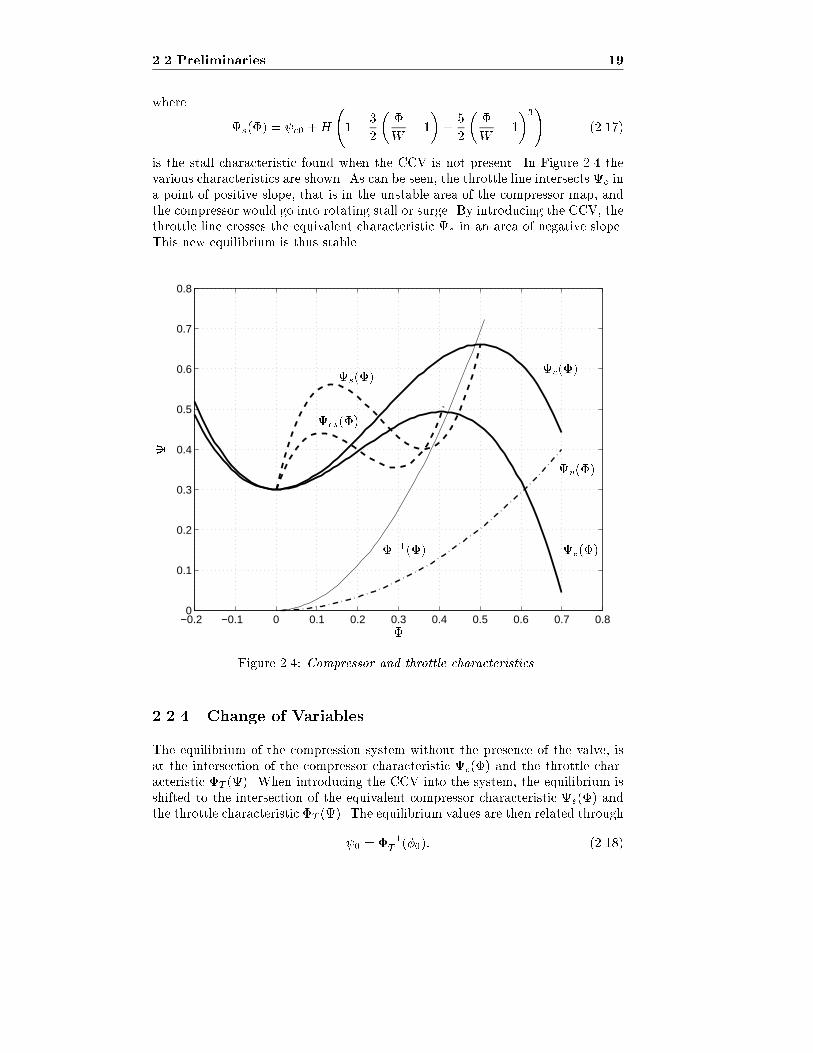
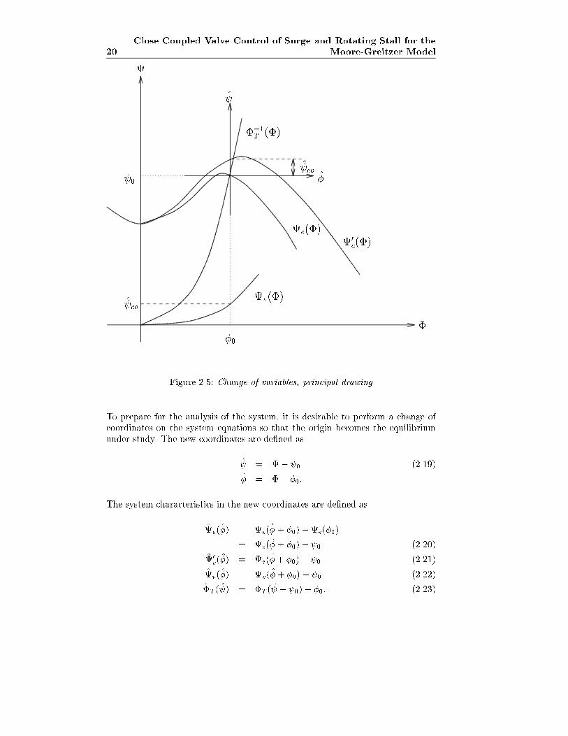
2.2.4 Change of Variables
The equilibrium of the compression system without the presence of the valve, isat the intersection of the compressor characteristic c(�) and the throttle char-acteristic �T (). When introducing the CCV into the system, the equilibrium isshifted to the intersection of the equivalent compressor characteristic e(�) andthe throttle characteristic �T (). The equilibrium values are then related through
0 = ��1T(�0): (2.18)
20
Close Coupled Valve Control of Surge and Rotating Stall for the
Moore-Greitzer Model
�
0
�0
�
v(�)
0c(�)
e(�)
��1T (�)
co
co
Figure 2.5: Change of variables, principal drawing
To prepare for the analysis of the system, it is desirable to perform a change ofcoordinates on the system equations so that the origin becomes the equilibriumunder study. The new coordinates are de�ned as
= � 0 (2.19)
� = �� �0:
The system characteristics in the new coordinates are de�ned as
e(�) = e(� + �0)�e(�0)
= e(� + �0)� 0 (2.20)
0c(�) = c(�+ �0)� 0 (2.21)
v(�) = v(�+ �0)� 0 (2.22)
�T ( ) = �T ( + 0)� �0: (2.23)
2.2 Preliminaries 21
Using (2.7), the transformed compressor characteristic (2.21) can be calculated as
0c(�) = co � k3�
3 � k2�2 � k1�; (2.24)
where
co = co � 0 � �20H
2W 2
��0
W� 3
�; (2.25)
k1 =3H�02W 2
��0
W� 2
�; (2.26)
k2 =3H
2W 2
��0
W� 1
�; (2.27)
k3 =H
2W 3: (2.28)
It can be recognized that k3 > 0, while k1 � 0 if the equilibrium is in the unstableregion of the compressor map and k1 > 0 otherwise. The sign of k2 may vary. If�0 > W then k2 > 0, and if �0 < W then k2 < 0.
Using the de�nition of the equivalent compressor (2.10) and the de�nition of 0in (2.18), it can be shown that
0 = co � �20H
2W 2
��0
W� 3
��v(�0): (2.29)
Combining (2.29) with (2.25) we get the simple result
co = v(�0); (2.30)
which could have been seen directly from Figure 2.5.
The Moore-Greitzer model (2.13) can now be written in the new coordinates as
_ =
1
4B2lc
��� �T ( )
�(2.31)
_� =
1
lc
�0c(�)� � v(�)� 0 � 3H
4J
��
W� 1
�� W 2J
2 2
�
_J = %J
"1�
��
W� 1
�2� J
4
#� 4W%
3H 2J�;
By de�ning0c(�) = v(�0) + c(�); (2.32)
where
c(�)4= �k3�3 � k2�
2 � k1�; (2.33)
the model (2.31) can be written
22
Close Coupled Valve Control of Surge and Rotating Stall for the
Moore-Greitzer Model
_ =
1
4B2lc
��� �T ( )
�(2.34)
_� =
1
lc
�c(�)� � u� 3H
4J
��
W� 1
�� W 2J
2 2
�
_J = %J
"1�
��
W� 1
�2� J
4
#� 4W%
3H 2J�;
where the control u has been selected as
u = v(�) + 0 �v(�0) = v(�)�v(�0): (2.35)
In the case of pure surge, the model (2.34) reduces to
_ =
1
4B2lc(�� �T ( )) (2.36)
_� =
1
lc(c(�)� u� )
Simon and Valavani (1991) suggested using the pressure drop across the valve asthe control variable u. This approach will also be taken here. Our aim will be todesign a control law u for the valve such that the compressor can be operated alsoon the left side of the original surge line without going into surge or rotating stall.That is, we are going to use feedback to move the surge line towards lower valuesof �, and thus expand the useful range of mass ows over which the compressorcan be safely operated.
As the pressure di�erence across the valve always will be a pressure drop, thevalve must be partially closed during stable operation in order for the control u toattain both positive and negative values. It is also evident that there must exista pressure drop over the valve when the compressor is operated in a previouslyunstable area. The price paid for a larger operating range, is some pressure lossat low mass ows. A further discussion of the steady state pressure loss can befound in Simon and Valavani (1991).
2.2.5 Disturbances
As in all types of physical systems, disturbances will occur in the compressionsystem. Greitzer and Moore (1986) stated that this is a topic that need morestudy, at least in the case of the disturbances initiating stall and surge. Someresearch have been done in this area. Hynes and Greitzer (1987), DeLaat et al.(1996) and others have studied the e�ect of circumferential inlet distortion on thestability properties, and Simon and Valavani (1991), Haddad et al. (1997) andothers studied mass ow and pressure disturbances. From a control theory pointof view it is also important to investigate what performance the closed loop systemwill have when disturbances is taken into account.
2.2 Preliminaries 23
As in Simon and Valavani (1991), the e�ect of a pressure disturbance d(�), anda ow disturbance �d(�) will be considered here. The pressure disturbance, whichmay arise from combustion induced uctuations when considering the model of agas turbine, will accelerate the ow. As pointed out by van de Wal and Willems(1996), the ow disturbances may arise from processes upstream of the compressor,other compressors in series or an air cleaner in the compressor duct. In the caseof an aircraft jet engine, large angle of attack or altitude variations may causemass ow disturbances according to van de Wal and Willems (1996) and DeLaatet al. (1996). Also, DeLaat et al. (1996) reports of a number of aircraft maneuvers(full-rudder sideslips, wind-up turns, etc.) causing inlet air ow disturbances inthe jet engine of a F-15 �ghter.
In the analysis of Simon and Valavani (1991) �d(�) is set to zero. Disturbancesin stall/surge control is also studied by Haddad et al. (1997), with disturbancesassumed to converge to zero. Here, both types of disturbances, mass ow andpressure, will be considered. The disturbances are time varying, and the onlyassumption made at this point is boundedness, that is k�dk1 and kdk1 exists.In addition to time varying disturbances, constant, or slow varying, o�sets will beintroduced into the model. This is of particular interest when e.g. a constant neg-ative mass ow disturbance pushes the equilibrium over the surge line, initiatingsurge or rotating stall. The o�sets in mass ow and pressure rise is termed d� andd , respectively. The constant bias d in pressure can also be thought of as re-
ecting some uncertainty in the compressor characteristic c(�), and likewise andthe mass ow bias d� can be thought of as re ecting a uncertainty in the throttle
characteristic �( ). A study of surge/stall control for compressors with uncertaincompressor characteristic was also done by Leonessa et al. (1997b). With thesedisturbances the model becomes:
_ =
1
4B2lc
��� �T ( )� �d(�)� d�
�(2.37)
_� =
1
lc
�� + c(�)� v(�) + d(�) + d
�3HJ
4
��
W� 1
�� W 2J
2 2
�
_J = %J
1�
��
W� 1
�2� J
4
!� 4W%
3H 2J�;
and in the case of pure surge
_ =
1
4B2lc
��� �T ( )� �d(�) � d�
�(2.38)
_� =
1
lc
�� + c(�)� v(�) + d(�) + d
�: (2.39)
24
Close Coupled Valve Control of Surge and Rotating Stall for the
Moore-Greitzer Model
2.3 Surge Control
In this section controllers will be designed for the pure surge case. First theundisturbed case is studied, then disturbances are added, and �nally adaption willbe used to stabilize the system in the presence of constant disturbances.
2.3.1 Undisturbed Case
Theorem 2.1 The controller
u = c2(�� �0); (2.40)
where c2 > am and am is the maximum positive slope of the compressor charac-
teristic c(�), renders the equilibrium (�0; 0) of (2.14) GAS. �
Proof: The backstepping methodology of Krsti�c et al. (1995a) will be employedin deriving the control law.
Step 1. Two error variables are de�ned as z1 = and z2 = � � �. The controlLyapunov function (clf) for this step is chosen as
V1 = 2B2lcz21 (2.41)
with time derivative along the solution trajectories of (2.36) given by
_V1 = z1
���T (z1) + z2 + �
�: (2.42)
The throttle is assumed passive, that is �T ( ) � 0 8 . We have
�T ( ) � 0 ) �z1�T (z1) � 0 (2.43)
As it is desirable to avoid cancelation of useful nonlinearities in (2.42), the stabi-lizing function � is not needed and accordingly � = 0, which gives
_V1 = ��T (z1)z1 + z1z2: (2.44)
Although the virtual control � is not needed here, in the interest of consistencywith the following sections, this notation is kept.
Step 2.The derivative of z2 is
_z2 =1
lc
�c(z2)� z1 � u
�: (2.45)
The clf for this step is
V2 = V1 +lc
2z22 (2.46)
2.3 Surge Control 25
with time derivative
_V2 = �z1�T (z1) + z2
�c(z2)� u
�: (2.47)
Notice that V2 as de�ned by (2.46) is similar to the incremental energy of Simonand Valavani (1991).
Control law. The control variable u will be chosen so that (2.47) is made negativede�nite. To this end we de�ne the linear control law
u = c2z2; (2.48)
where the controller gain c2 > 0 is chosen so that
z2c(z2)� c2z22 < 0: (2.49)
Using (2.33) this implies that c2 must satisfy
�k3z22�z22 +
k2
k3z2 +
k1 + c2
k3
�< 0: (2.50)
Finding the roots of the above bracketed expression, it is seen that (2.50) is satis�edif c2 is chosen according to
c2 >k224k3
� k1: (2.51)
Although (2.51) implies that the compressor characteristic must be known in orderto determine c2, it can be shown that the knowledge of a bound on the positiveslope of the characteristic is su�cient. Di�erentiating (2.33) twice with respect to
�, reveals that the maximum positive slope occurs for
� = �m = � k2
3k3(2.52)
and is given by
a =dc(�)
d�
������=�m
=k223k3
� k1 =3H
2W: (2.53)
Assuming that only an upper bound am on the positive slope of c(�) is known,a conservative condition for c2 is
c2 > am � a >k224k3
� k1: (2.54)
Thus the price paid for not knowing the exact coe�cients of the compressor char-acteristic is a somewhat conservative condition for the controller gain c2. Noticealso that no knowledge of Greitzer's B-parameter or its upper bound is requiredin formulating the controller. The �nal expression for _V2 is then
_V2 = �z1�T (z1) + c(z2)z2 � c2z22 = �W (z1; z2) � 0: (2.55)
26
Close Coupled Valve Control of Surge and Rotating Stall for the
Moore-Greitzer Model
The closed loop system can be written as
_z1 =1
4B2lc(��T (z1) + z2) (2.56)
_z2 =1
lc(�z1 + (z2)� c2z2): (2.57)
It follows that the equilibrium point z1 = z2 = 0 is GAS, and the same resultholds for the equilibrium (�0; 0). �
Remark 2.1 By combining (2.82) and (2.48), the following control law for the
CCV gain is found:
c2(�� �0) = v(�)�v(�0) (2.58)
+
=
r�+ �0
c2: (2.59)
Notice that this control law requires measurement of mass ow only. �
Remark 2.2 Although not showing stability, Bendixon's criterion can be used to
show that the controller (2.48) guarantees that no limit cycles (surge oscillations)
exists. Bendixon's criterion states (somewhat simpli�ed) that no limit cycles ex-
ists in a dynamical system de�ned on a simply connected region D � IIR2 if the
divergence of the system is not identically zero and does not change sign in D. For
an exact statement of Bendixon's criterion and the proof, see any textbook on dy-
namical systems, e.g. Perko (1991). The divergence r �f of the system _x = f (x)de�ned by (2.14) is
r � f = � 1
4B2lc
@�T ( )
@ +
1
lc
@ c(�)
@�� @u
@�
!: (2.60)
The slope of the throttle is always positive, so the �rst term in (2.60) is always
negative. To make the second term also negative, it is su�cient that @u@�
dominates
@ c(�)
@�, which is exactly what is ensured by the controller in Theorem 2.1. Thus,
according to Bendixon's criterion, no surge oscillations can exist for the closed
loop system. �
2.3.2 Determination of �0
As a consequence of the controller (2.40) being designed after the system equationsare transformed to the new coordinates, its implementation depends on knowledgeof the equilibrium value �0. The equilibrium is located at the intersection of the
2.3 Surge Control 27
equivalent compressor characteristic e(�) and the throttle characteristic ��1T.
By combining (2.82), (2.40) and (2.59), it is seen that
v(�0) = (u+v(�0))j�=�0=
�c2(�� �0) +
c2
�+ �0�20
������=�0
=c2�0
2: (2.61)
At the equilibrium, we have
c(�0)�v(�0) =1
2�20; (2.62)
or by using (2.61), �0 is found by solving the following 3rd order equation
co +H
1 +
3
2
��0
W� 1
�� 1
2
��0
W� 1
�3!� c2�0
2=
2
2�20; (2.63)
with respect to �0, and its value is to be used in the control law (2.40). Solving(2.63) requires knowledge of the compressor characteristic. If this is not the case,alternatives to �nding �0 explicitly is, using an adaption scheme like the onesuggested by Bazanella et al. (1997) or it is possible to use throttle control inaddition to the CCV control to control � using �0 as the reference. If none ofthese alternatives are attractive, an approximation for �0 can be used. In this case,asymptotic stability cannot be shown, but convergence to a set and avoidance ofsurge is easily shown. De�ning �� as
�� = �0 � �aprx; (2.64)
where �aprx is the approximation used for feedback, and �0 is the actual andunknown value of the equilibrium. By using the same Lyapunov function as isTheorem 2.1, and
u = c2(�� �aprx) = c2(�� �0 +��); (2.65)
the time derivative of V2 is found and upper bounded by
_V2 � �z1�(z1) + z2(c(z2)� c2z2)z2 � z2c2��: (2.66)
Application of Young's inequality4 to the last term in (2.66) gives
�z2c2�� � c2
2
�z22�0
+ (��)2�0
�; (2.67)
4In its simplest form Young's inequality states that
8a; b : ab �1
2(a2
c+ cb2) 8c > 0:
28
Close Coupled Valve Control of Surge and Rotating Stall for the
Moore-Greitzer Model
where �0 is a constant, and it follows that
_V2 � �z1�T (z1) + z2(c(z2)� c2(1� 1
2�0)z2)z2 + �0(��)
2
= �W (z1; z2) + �0(��)2; (2.68)
where the de�nition of W is obvious. By choosing �0 and c2 such that
c2(1� 1
2�0) > am; (2.69)
is satis�ed, it can be shown thatW (z1; z2) is radially unbound and positive de�nite.Thus, _V2 < 0 outside a set R�. This set can be found in the following manner:According to Krsti�c et al. (1995a), the fact that V2(z1; z2) andW (z1; z2) is positivede�nite and radially unbounded, and V2(z1; z2) is smooth, implies that there existsclass-K1 functions �1, �2 and �3 such that
�1(jzj) � V2(z) � �2(jzj) (2.70)
�3(jzj) � W (z) (2.71)
where z = (z1 z2)T. Following the proof of Lemma 2.26 in Krsti�c et al. (1995a),
we have that the states of the model are uniformly ultimately bounded, and thatthey converge to the residual set
R� =
(z : jzj � ��11 � �2 � ��13
��(��)2
�): (2.72)
From (2.68) it follows that _V2 is negative whenever W (z) > �0(��)2. Combining
this with (2.71) it can be concluded that
jz(�)j > ��13
��(��)2
� ) _V2 < 0: (2.73)
This means that if jz(0)j � ��13
��(��)2
�, then
V2(z(�)) � �2 � ��13
��(��)2
�; (2.74)
which in turn implies that
jz(�)j � ��11 � �2 � ��13
��(��)2
�: (2.75)
If, on the other hand jz(0)j > ��13
��(��)2
�, then V2(z(�)) � V2(z(0)), which
impliesjz(�)j � ��11 � �2(jz(0)j): (2.76)
Combining (2.75) and (2.76) leads to the global uniform boundedness of z(�):
kzk1 � max���11 � �2 � ��13
��(��)2
�; ��11 � �2(jz(0)j)
; (2.77)
while (2.73) and (2.70) prove the convergence of z(�) to the residual set de�nedin (2.72).
It is trivial to establish the fact that no limit cycles, and hence surge oscillations,can exist inside this set using Bendixon's criterion. It is seen from (2.72), that thesize of the set R� is dependent on the square of the equilibrium estimate error ��and the parameter �0. A more accurate estimate �aprx, or a smaller value of �0,both implies a smaller set. A smaller value of �0 will, by equation (2.69), requirea larger controller gain c2, which is to be expected.
2.3 Surge Control 29
2.3.3 Time Varying Disturbances
First, time varying pressure disturbances will be considered. That is, �d(�), d�and d are set to zero as in Simon and Valavani (1991).
Theorem 2.2 (Time varying pressure disturbances)
The controller
u = (c2 + d2)(�� �0); (2.78)
where c2 is chosen as in Theorem 2.1, and d2 > 0 guarantees that the states of themodel (2.38) are globally uniformly bounded, and that they converge to a set. �
Proof: The controller will be derived using backstepping.
Step 1. Identical to Step 1 in proof of Theorem 2.1.
Step 2. The derivative of z2 is
_z2 =1
lc
�c(�)� z1 + d(�)� u
�: (2.79)
V2 is chosen as
V2 = V1 +lc
2z22 (2.80)
where _V2 can be bounded according to
_V2 = ��T (z1)z1 + z2
�c(�) + d(�)� u
�: (2.81)
Control law. To counteract the e�ect of the disturbance, a damping factor d2 > 0is included and u is chosen as
u = c2z2 + d2z2: (2.82)
c2 is chosen so that (2.54) is satis�ed. Inserting (2.82) in (2.81) gives
_V2 = �z1�T (z1) + c(z2)z2 � c2z22 + d(�)z2 � d2z
22 : (2.83)
Use of Young's inequality gives
z2d(�) � d2z22 +
2d(�)
4d2� d2z
22 +
kdk214d2
; (2.84)
and _V2 can be bounded according to
_V2 � �W (z1; z2) +2d(�)
4d2� �W (z1; z2) +
1
4d2kdk21 (2.85)
30
Close Coupled Valve Control of Surge and Rotating Stall for the
Moore-Greitzer Model
whereW (z1; z2) = z1�(z1)� (c(z2)z2 � c2z
22) (2.86)
is radially unbounded and positive de�nite. This implies that _V2 < 0 outside a setR1 in the z1z2 plane.
By using (2.70) and (2.71) again, it follows from similar calculations as in (2.73)-(2.77), that z(�) is globally uniformly bounded and that z(�) converges to theresidual set
R1 =
(z : jzj � ��11 � �2 � ��13
kdk214d2
!): (2.87)
�
Remark 2.3 Notice that the controller (2.82) is essentially the same as (2.48),
with the only di�erence being that (2.82) requires a larger gain in order to suppress
the disturbance. Consequently, Remark 2.1 also applies here. �
It is now shown that an additional assumption on the disturbance ensures thatthe controller (2.82) not only makes the states globally uniformly bounded, butalso guarantees convergence to the origin.
Corollary 2.1 (Convergence to the origin)
If the disturbance term d(�) is upper bounded by a monotonically decreasing
non-negative function d(�) such that
jd(�)j � d(�) 8� � 0 (2.88)
and
lim�!1
d(�) = 0; (2.89)
the controller (2.82) ensures that the states of the model (2.38), with pressure dis-
turbances, converge to the origin. �
Proof: Inspired by the calculations for a simple scalar system starting on page 75in Krsti�c et al. (1995a) , we introduce the signal
s(z; �) = V2(z)ec�; (2.90)
where c > 0 is a constant, for use in the proof:
d
dts(z; �) =
d
dt
�V2(z)e
c�
=�_V2(z) + cV2(z)
�ec�
� �W (z) +
2d(�)
4d2+ cV2(z)
!ec�
� (��3(jzj) + c�2(jzj)) ec� + 2d(�)
4d2ec�: (2.91)
2.3 Surge Control 31
By choosing c according to
c � ��12 � �3(jzj) � ��12 � �3(kzk1); (2.92)
where the existence of kzk1 follows from (2.87), (2.91) gives
d
dt
�V2(z)e
c� � 2
d(�)
4d2ec�: (2.93)
By integrating (2.93) and using an argument similar to the one in the proof oflemma 2.24 in Krsti�c et al. (1995a), it can be shown that
V2(z(�)) � V2(z(0))e�c� +
1
4cd2
�d
2(0)e�
c�
2 +d2(�=2)
�: (2.94)
Since lim�!1d2(�=2) = 0 it follows that
lim�!1
V2(z(�)) = 0: (2.95)
As V2 is positive de�nite it follows that
lim�!1
z(�) = 0: (2.96)
Thus we have shown that under the additional assumptions (2.88) and (2.89) on
the disturbance term, z(�) converges to the origin. This also implies that � and converge to the origin and that �(�) and (�) converge to the point of intersectionof the compressor and throttle characteristic. �
Notice that the positive constant c introduced in (2.90) is used for analysis only,and is not included in the implementation of the control law.
At this point we include the ow disturbance �d(�) in the analysis.
Theorem 2.3 (Time varying pressure and ow disturbances)
The controller
u = c2z2 � k3��3 + 3�z22
�� k2�2 � k1�
+d1
4B2
���T (z1) + �
�+ d2z2
�1 +
d214B2
�; (2.97)
where c2 > jk1j guarantees that the states of the model (2.37) with both mass ow
disturbances and pressure disturbances is globally uniformly bounded and that they
converge to a set. �
Proof: The backstepping procedure is as follows:
32
Close Coupled Valve Control of Surge and Rotating Stall for the
Moore-Greitzer Model
Step 1. As before two error variables z1 and z2 are de�ned as z1 = and z2 = ���.Again, V1 is chosen as
V1 = 2B2lcz21 ; (2.98)
with time derivative
_V1 = z1
���T (z1) + z2 � �d(�) + �
�; (2.99)
where (2.37) is used. The virtual control � is chosen as
� = �d1z1; (2.100)
where �d1z1 is a damping term to be used to counteract the disturbance �d(�)._V1 can now be written as
_V1 = �d1z21 + z1z2 � �d(�)z1 � �T (z1)z1; (2.101)
and upper bounded according to
_V1 � ��T (z1)z1 + z1z2 +k�dk214d1
: (2.102)
To obtain the bound in (2.102), Young's inequality has been used to obtain
��d(�)z1 � d1z21 +
�2d(�)
4d1� d1z
21 +
k�dk214d1
: (2.103)
Step 2. The derivative of z2 is
_z2 =1
lc
�c(�)� z1 + d(�)� @�
@z1
1
4B2lc
���T (z1) + �
�
+1
4B2lc
@�
@z1�d(�)� u
�: (2.104)
From (2.100) it is seen that@�
@z1= �d1: (2.105)
V2 is chosen as
V2 = V1 +lc
2z22 : (2.106)
Using (2.102) and (2.104), an upper bound on _V2 is
_V2 � ��T (z1)z1 + k�dk214d1
+ z2
�c(�) + d(�)
+d1
4B2
���T (z1) + �
�� d1
4B2�d(�)� u
�: (2.107)
Control law. To counteract the e�ect of the disturbances, a damping factor d2must be included and u is chosen as
u = c2z2 � k3��3 + 3�z22
�� k2�2 � k1�
+d1
4B2
���T (z1) + �
�+ d2z2
�1 +
d214B2
�: (2.108)
2.3 Surge Control 33
The parameter c2 is now chosen according to
c2 > jk1j: (2.109)
Inserting (2.97) in (2.107) gives
_V2 � �(c2 + k1)z22 � k3(z
42 + 3�2z22)� �T (z1)z1 +
k�dk214d1
�d2z22 + jz2jkdk1 +d1
4B2jz2jk�dk1 � d21
4B2d2z
22 : (2.110)
Using Young's inequality twice gives
jz2jkdk1 � d2z22 +
kdk214d2
(2.111)
d1
4B2jz2jk�dk1 � 1
4B2
d21d2z
22 +
k�dk214d2
!: (2.112)
The �nal upper bound for V2 can now be written as
_V2 � �W (z1; z2) +1
�1k�dk21 +
1
�2kdk21 (2.113)
where1
�1=
�1
4d1+
1
16B2d2
�;1
�2=
1
4d2(2.114)
andW (z1; z2) = (c2 + k1)z
22 + k3(z
42 + 3�2z22) + �(z1)z1 (2.115)
is radially unbounded and positive de�nite. This implies that _V2 < 0 outside a setR2 in the z1z2 plane. As in section 6.1, the functions V2(z) and W (z) exhibit theproperties in (2.70). Again, it can be shown that this implies that z(�) is globallyuniformly bounded and that z(�) converges to the residual set
R2 =
(z : jzj � ��11 � �2 � ��13
kdk21�1
+k�dk21�2
!): (2.116)
�
Remark 2.4 Notice that the control law (2.97), as opposed to (2.82), requires
knowledge of the coe�cients in the compressor characteristic, the throttle charac-
teristic and the B-parameter. �
Remark 2.5 Once the bounds on the disturbances k�dk1 and kdk1 are known,
the size of the set R2 in the z1z2 plane can be made arbitrary small by choosing
the damping factors d1 and d2 su�ciently large. The same comment applies to the
set R1 de�ned in (2.87). �
34
Close Coupled Valve Control of Surge and Rotating Stall for the
Moore-Greitzer Model
Corollary 2.2 (Convergence to the origin)
If the assumptions on d(�) in equations (2.117) and (2.118) hold, and the fol-
lowing assumption on �d(�) is made:
j�d(�)j � �d(�) 8� � 0 (2.117)
and
lim�!1
�d(�) = 0; (2.118)
where �d(�) is a monotonically decreasing non-negative function. Then, the statesof the model (2.38) converge to the origin. �
Proof: By using the same arguments as in the proof of Corollary 2.1, but withtwo disturbance terms, it can be shown that
V2(z(�)) � V2(z(0))e�c� +
1
c�1
��d
2(0)e�
c�
2 +�d2(�=2)
�+
1
c�2
�d
2(0)e�
c�
2 +d2(�=2)
�: (2.119)
Now lim�!1d2(�=2) = 0 and lim�!1 �d
2(�=2) = 0 implies that
lim�!1 V2(z(�)) = 0 and by the positive de�niteness of V2 it follows that
lim�!1
z(�) = 0: (2.120)
Thus we have shown that under the assumptions (2.88), (2.89), (2.117) and (2.118)
on the disturbance terms, z(�) converge to the origin. This also implies that �(�)
and (�) converges to the origin and that �(�) and (�) converge to the point ofintersection of the compressor and throttle characteristic. �
A simulation of the response of the control law (2.97) with both mass ow andpressure disturbances is presented in Chapter 3, where it is compared to a passivitybased controller.
2.3.4 Adaption of Constant Disturbances
A constant or slow varying disturbance in mass ow can cause the equilibriumof the compression system to be moved into the unstable area of the compressormap. Therefore, the problem of being able to stabilize the system in this case isa very important one. In addition constant disturbances in pressure is consideredsimultaneously. Consider the following model
_ =
1
4B2lc
��� �T ( )� d�
�_� =
1
lc
�c(�)� + d � u
�; (2.121)
2.3 Surge Control 35
where d� and d are constant and unknown disturbances in mass ow and pres-sure, respectively. Godhavn (1997) used adaptive backstepping for adaption ofconstant or slow varying sea current disturbances in a surface ship model. Thesame approach will now be employed here to stabilize (2.121). Two adaption lawswill be designed in order to estimate the unknown disturbances and allow themto be counteracted by the control.
Theorem 2.4 The controller
u =lc
#1z1 + c2z2 � k3
�d3
�+ 3d�z
22
�� k2�
2 � k1d� + d ; (2.122)
where the estimates d� and d are updated with
_d� = � 1
#1z1 (2.123)
_d = � 1
#2z2; (2.124)
where 1#1
and 1#2
are adaption gains, makes the equilibrium of (2.121) globally
asymptotically stable. The states of the model converge to their equilibrium values
and the parameter error dynamics are GAS. asymptotically stable. �
Proof: Backstepping is used
Step 1. The error variables z1 and z2 are de�ned as z1 = and z2 = � � �. The�rst clf, V1, is chosen as
V1 = 2B2lcz21 +
#1
2~d2�; (2.125)
where~d�
4= d� � d�; (2.126)
is the parameter error and d� is an estimate of d�. The time derivative of V1 nowis
_V1 = z1
���T (z1) + z2 � d� + �
�� #1 ~d�
_d�; (2.127)
where (2.121) is used. Let the virtual control � be chosen as
� = d�; (2.128)
and the estimate d� be updated as
_d� = � 1
#1z1: (2.129)
Thus, the terms including ~d� in (2.127) are cancelled out, and _V1 can now bewritten as
_V1 = z1z2 � �T (z1)z1: (2.130)
36
Close Coupled Valve Control of Surge and Rotating Stall for the
Moore-Greitzer Model
Step 2. The second clf is chosen as
V2 = V1 +lc
2z22 +
#2
2~d2 =
1
2zTPz +
1
2~dT��1~d; (2.131)
where~d
4= d � d ; (2.132)
is the parameter error, d is an estimate of d ,
~d = ( ~d� ~d ); P =
�4B2lc 00 lc
�; and ��1 =
�#1 00 #2
�: (2.133)
Using (2.121), _V2 is calculated as
_V2 = ��(z1)z1 + z2(c(�)� u+lc
#1z1 + d )� #2 ~d
_d : (2.134)
Let the estimate d be updated as
_d =1
#2z2; (2.135)
and the control be chosen as
u =lc
#1z1 + c2z2 � k3
��3 + 3�z22
�� k2�2 � k1�+ d : (2.136)
Using the calculations from the case of time varying disturbances it can be shownthat _V2 can be upper bounded as
_V2 � �(c2 + k1)z22 � k3(z
42 + 3�2z22)� �T (z1)z1 (2.137)
By inserting the update laws (2.129) and (2.135) and the control (2.136) in equa-tions (2.121), it can be shown that the error dynamics get the following form
_z = P�1�Az(z;d) +P zz + ~d
�(2.138)
_~d = ��z; (2.139)
where
Az(z;d) =
���T (z1)
�c2z2 � k3(z32 + 3�2z2)
�and P z =
�0 1�1 0
�: (2.140)
The stability result follows from application of LaSalle's theorem. From (2.137) itis seen that
_V2 � 0) z � 0) _z � 0: (2.141)
Inserting (2.141) into (2.138) we �nd that ~d � 0. Thus the origin of (2.138) isGAS. �
This result could also have been stated by using the more general Theorem 4.12in Krsti�c et al. (1995a) or the results in Krsti�c (1996).
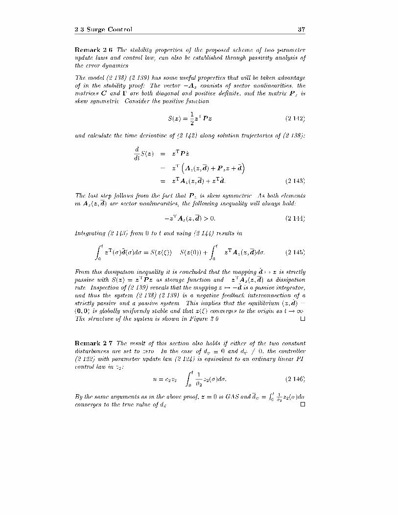
2.3 Surge Control 37
Remark 2.6 The stability properties of the proposed scheme of two parameter
update laws and control law, can also be established through passivity analysis of
the error dynamics.
The model (2.138)-(2.139) has some useful properties that will be taken advantage
of in the stability proof: The vector �Az consists of sector nonlinearities, the
matrices C and � are both diagonal and positive de�nite, and the matrix P z is
skew symmetric. Consider the positive function
S(z) =1
2zTPz (2.142)
and calculate the time derivative of (2.142) along solution trajectories of (2.138):
d
dtS(z) = zTP _z
= zT�Az(z;d) +P zz + ~d
�= zTAz(z;d) + z
T~d: (2.143)
The last step follows from the fact that P z is skew symmetric. As both elements
in Az(z;d) are sector nonlinearities, the following inequality will always hold:
�zTAz(z;d) > 0: (2.144)
Integrating (2.143) from 0 to t and using (2.144) results in
Zt
0
zT(�)~d(�)d� = S(z(�))� S(z(0)) +
Zt
0
�zTAz(z;d)d�: (2.145)
From this dissipation inequality it is concluded that the mapping ~d 7! z is strictly
passive with S(z) = zTPz as storage function and �zTAz(z;d) as dissipation
rate. Inspection of (2.139) reveals that the mapping z 7! �~d is a passive integrator,
and thus the system (2.138)-(2.139) is a negative feedback interconnection of a
strictly passive and a passive system. This implies that the equilibrium (z; ~d) =(0;0) is globally uniformly stable and that z(�) converges to the origin as t!1.
The structure of the system is shown in Figure 2.6. �
Remark 2.7 The result of this section also holds if either of the two constant
disturbances are set to zero. In the case of d� � 0 and d 6= 0, the controller
(2.122) with parameter update law (2.124) is equivalent to an ordinary linear PI-
control law in z2:
u = c2z2 �Zt
0
1
#2z2(�)d�: (2.146)
By the same arguments as in the above proof, z = 0 is GAS and d =Rt
01#2z2(�)d�
converges to the true value of d . �
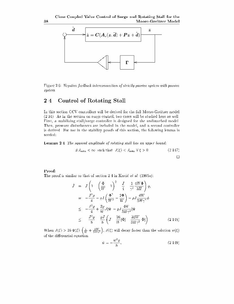
38
Close Coupled Valve Control of Surge and Rotating Stall for the
Moore-Greitzer Model
h
,,,lll
~d z
�
_z = C(Az(z;d) + Pz + ~d)
�
Figure 2.6: Negative feedback interconnection of strictly passive system with passive
system
2.4 Control of Rotating Stall
In this section CCV controllers will be derived for the full Moore-Greitzer model(2.34). As in the section on surge control, two cases will be studied here as well.First, a stabilizing stall/surge controller is designed for the undisturbed model.Then, pressure disturbances are included in the model, and a second controlleris derived. For use in the stability proofs of this section, the following lemma isneeded:
Lemma 2.1 The squared amplitude of rotating stall has an upper bound:
9 Jmax <1 such that J(�) < Jmax 8 � > 0 (2.147)
�
Proof:
The proof is similar to that of section 2.4 in Krsti�c et al. (1995a):
_J = J
1�
��
W� 1
�2� J
4� 1
24W�
3H
!%;
= �J2%
4� %J
��2
W 2� 2�
W
�� %J
4W
3H 2�
� �J2%
4+
2%
WJ j�j+ %J
4W
3H 2j�j
� �J2%
8� %J
8
�J � 16
Wj�j � 32W
3H 2j�j�
(2.148)
When J(�) > 16j�(�)j�
1W
+ 2W3H 2
�, J(�) will decay faster than the solution w(�)
of the di�erential equation
_w = �w2%
8; (2.149)
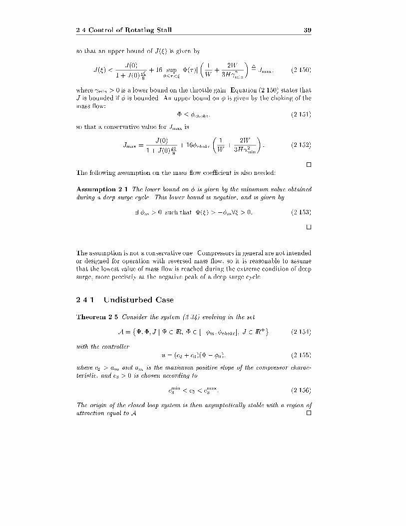
2.4 Control of Rotating Stall 39
so that an upper bound of J(�) is given by
J(�) <J(0)
1 + J(0)%�8
+ 16 sup0��<�
j�(�)j�
1
W+
2W
3H 2min
�4= Jmax; (2.150)
where min > 0 is a lower bound on the throttle gain. Equation (2.150) states thatJ is bounded if � is bounded. An upper bound on � is given by the choking of themass ow:
� � �choke; (2.151)
so that a conservative value for Jmax is
Jmax =J(0)
1 + J(0)%�8
+ 16�choke
�1
W+
2W
3H 2min
�: (2.152)
�
The following assumption on the mass ow coe�cient is also needed:
Assumption 2.1 The lower bound on � is given by the minimum value obtained
during a deep surge cycle. This lower bound is negative, and is given by
9 �m > 0 such that �(�) > ��m8� > 0: (2.153)
�
The assumption is not a conservative one. Compressors in general are not intendedor designed for operation with reversed mass ow, so it is reasonable to assumethat the lowest value of mass ow is reached during the extreme condition of deepsurge, more precisely at the negative peak of a deep surge cycle.
2.4.1 Undisturbed Case
Theorem 2.5 Consider the system (2.34) evolving in the set
A =�;�; J j 2 IIR; � 2 [��m; �choke]; J 2 IIR+
(2.154)
with the controller
u = (c2 + c3)(�� �0); (2.155)
where c2 > am and am is the maximum positive slope of the compressor charac-
teristic, and c3 > 0 is chosen according to
cmin3 < c3 < cmax3 : (2.156)
The origin of the closed loop system is then asymptotically stable with a region of
attraction equal to A. �
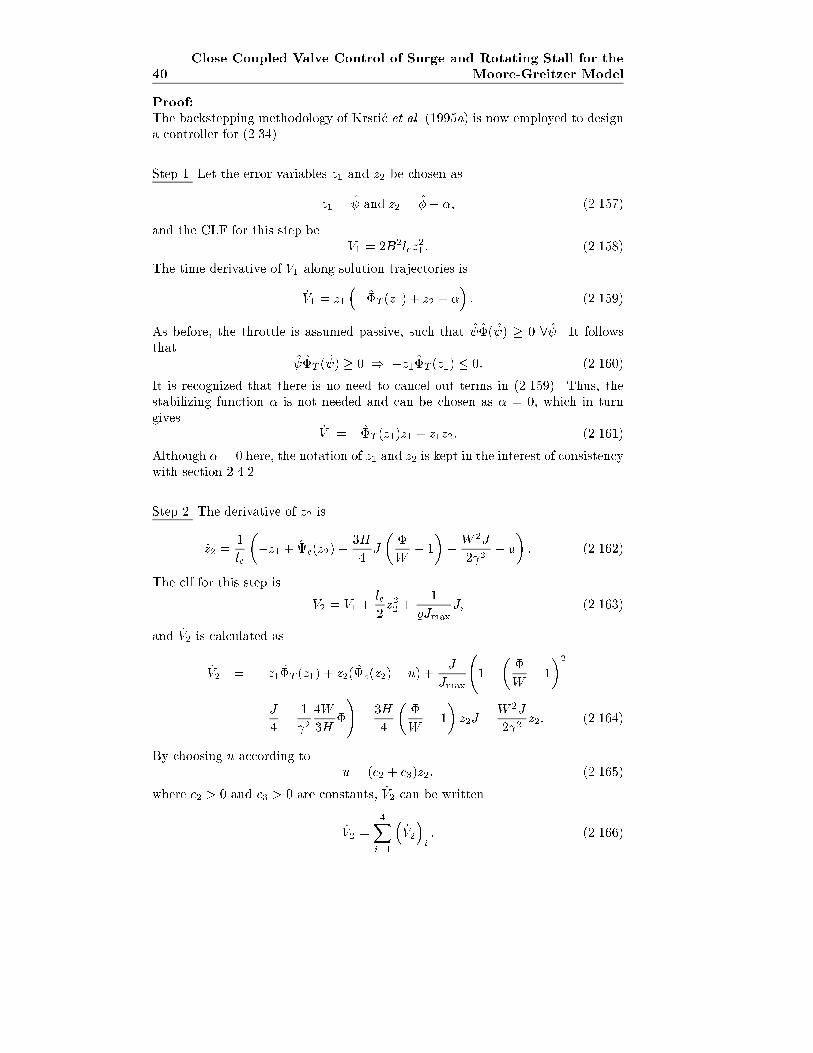
40
Close Coupled Valve Control of Surge and Rotating Stall for the
Moore-Greitzer Model
Proof:
The backstepping methodology of Krsti�c et al. (1995a) is now employed to designa controller for (2.34)
Step 1. Let the error variables z1 and z2 be chosen as
z1 = and z2 = �� �; (2.157)
and the CLF for this step beV1 = 2B2lcz
21 : (2.158)
The time derivative of V1 along solution trajectories is
_V1 = z1
���T (z1) + z2 + �
�: (2.159)
As before, the throttle is assumed passive, such that �( ) � 0 8 . It followsthat
�T ( ) � 0 ) �z1�T (z1) � 0: (2.160)
It is recognized that there is no need to cancel out terms in (2.159). Thus, thestabilizing function � is not needed and can be chosen as � = 0, which in turngives
_V1 = ��T (z1)z1 + z1z2: (2.161)
Although � = 0 here, the notation of z1 and z2 is kept in the interest of consistencywith section 2.4.2
Step 2. The derivative of z2 is
_z2 =1
lc
��z1 + c(z2)� 3H
4J
��
W� 1
�� W 2J
2 2� u
�: (2.162)
The clf for this step is
V2 = V1 +lc
2z22 +
1
%JmaxJ; (2.163)
and _V2 is calculated as
_V2 = �z1�T (z1) + z2(c(z2)� u) +J
Jmax
1�
��
W� 1
�2
�J4� 1
24W
3H�
!� 3H
4
��
W� 1
�z2J � W 2J
2 2z2: (2.164)
By choosing u according tou = (c2 + c3)z2; (2.165)
where c2 > 0 and c3 > 0 are constants, _V2 can be written
_V2 =
4Xi=1
�_V2
�i
: (2.166)
2.4 Control of Rotating Stall 41
The four terms in (2.166) are�_V2
�1
= �z1�T (z1); (2.167)�_V2
�2
= z2(c(z2)� c2z2); (2.168)
�_V2
�3
=J
Jmax
1�
��
W� 1
�2� 1
24W
3H�
!; (2.169)
�_V2
�4
= � � J z2�P (�)
�J
z2
�; (2.170)
where
P (�) =
"1
4Jmax
3H8
��W� 1�+ W
2
4 2
3H8
��W� 1�+ W
2
4 2c3
#: (2.171)
Due to the passivity of the throttle,�_V2
�1< 0. As shown in section 2.3, if c2 is
chosen as
c2 > am � a >k224k3
� k1; (2.172)
where am is the maximum positive slope of the compressor characteristic, then�_V2
�2< 0.
By choosing the controller gains su�ciently large,�_V2
�3can be made negative
for � > 0. As the proposed controller (2.165) is of the same form as (2.40), the
expression (2.59) for , with gain (c2+ c3), can be used. For�_V2
�3to be negative
the following must be satis�ed
1���
W� 1
�2� 4W
3H
�(c2 + c3)
� + �0< 0 (2.173)
+ � > 0
c2 + c3 >3H
4W
�+ �0
�
���
W� 1
�2+ 1
!(2.174)
c2 + c3 >3H
4W(� + �0)
�2
W� �
W 2
�4= G1(�) (2.175)
Simple calculations shows that the maximum of G1(�) is reached for � =W � �0
2.
The maximum is given by
max�>0
G1(�) =3H
4W 2
��204W
+W + �0
�: (2.176)
By choosing
c2 + c3 >3H
4W 2
��204W
+W + �0
�; (2.177)
42
Close Coupled Valve Control of Surge and Rotating Stall for the
Moore-Greitzer Model
which implies
c3 >3H
4W 2
��204W
+W + �0
�� c2
4= C1(c2); (2.178)
it follows that�_V2
�3is made negative for � > 0.
For � < 0 the sum�_V2
�3+�_V2
�2can be made negative for � > ��m, that is
z2(c(z2)� c2z2) < � J
Jmax
1�
��
W� 1
�2� 1
24W
3H�
!(2.179)
Using (2.59) and J
Jmax< 1, and rearranging (2.179) gives
c3
� + �0� > G2(�; c2); (2.180)
where
G2(�; c2)4=
4W
3H
z2c(z2)� c2z
22 + 1�
��
W� 1
�2!� c2
�+ �0�: (2.181)
It can be shown that it is su�cient that (2.180) is satis�ed at the end points ofthe interval:
G2(��m; c2) <�m
�m � �0c3 (2.182)
G2(0; c2) < 0: (2.183)
By inspection of (2.181) it is easily shown that (2.183) is always satis�ed. It isassumed that �0 > �m, so that the condition in (2.182) can be rewritten as
c3 <�m � �0
�mG2(��m; c2) 4= C2(c2; �m): (2.184)
Plots of�_V2
�2,�_V2
�3and their sum are shown in Figure 2.7.
Finally, c3 must be chosen so that P is positive de�nite for ��m < � < �choke.The determinant of P is given by
detP =c3
4Jmax��3H
8
��
W� 1
�+W 2
4 2
�2> 0: (2.185)
A plot of detP is shown in the lower part of Figure 2.7. Again, a su�cientcondition for detP > 0 for ��m < � < �choke is that detP (�choke) > 0 anddetP (��m) > 0. As shown in Appendix E, this leads to the following conditionson c3:
maxnC3(c2; �choke); C4(c2; �m)
o< c3 < min
nC3(c2; �choke); C4(c2; �m)
o(2.186)
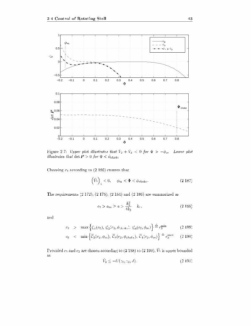
2.4 Control of Rotating Stall 43
−0.2 −0.1 0 0.1 0.2 0.3 0.4 0.5 0.6 0.7 0.8
−0.5
0
0.5
1
−0.2 −0.1 0 0.1 0.2 0.3 0.4 0.5 0.6 0.7 0.80
0.02
0.04
0.06
0.08
0.1
choke
��m
�
�
�
_ V
_V2
_V3
_V2 + _V3
detP
Figure 2.7: Upper plot illustrates that _V2 + _V3 < 0 for � > ��m. Lower plot
illustrates that detP > 0 for � < �choke.
Choosing c3 according to (2.186) ensures that�_V2
�4< 0; ��m < � < �choke: (2.187)
The requirements (2.172), (2.178), (2.184) and (2.186) are summarized as
c2 > am � a >k224k3
� k1; (2.188)
and
c3 > maxnC1(c2); C3(c2; �choke); C4(c2; �m)
o4= cmin3 (2.189)
c3 < minnC2(c2; �m); C3(c2; �choke); C4(c2; �m)
o4= cmax3 (2.190)
Provided c2 and c3 are chosen according to (2.188) to (2.190), _V2 is upper boundedas
_V2 � �U(z1; z2; J): (2.191)
44
Close Coupled Valve Control of Surge and Rotating Stall for the
Moore-Greitzer Model
As V2 : A ! IIR, V2(0) = 0, V2 is positive de�nite and continuously di�erentiableon A, and _V (z) < 0 for z 2 A � f0g, the origin of the system is asymptoticallystable with region of attraction equal to A. �
By doing the same calculations as in Remark 2.1, the control law for the CCVgain is found to be:
=
s�+ �0
(c2 + c3): (2.192)
Notice that this control law requires sensing of mass ow � only. The analysisleading to this control law was conservative, resulting in a large value of the pa-rameter c3, that is c3 has to be chosen as c3 > cmin3 . As was the case in Krsti�c etal. (1995b), the controller should be implemented with a lower gain than dictatedby the Lyapunov analysis. Consider the closed loop Jacobian of the model (2.34)with control law (2.155):
Acl =
0B@
� 14B2lc
a�1
4B2lc0
� 1lc� 3H
4lcW1lca � c2+c3
lc0
0 0 %�� �
20
W 2 +2�0W
�� 4W%(c2+c3)
6H
1CA ; (2.193)
where
a =@�T (z1)
@z1
�����z1=0
and a� =@c(z2)
@z2
�����z2=0
: (2.194)
It can be shown that if Acl is Hurwitz for c3 > cmin3 , Acl is also Hurwitz for c3 = 0.The closed loop system is therefore locally stable with c3 = 0.
2.4.2 Disturbed Case
The backstepping procedure is now used to design a controller that ensures bound-edness of the states in the presence of pressure disturbances.
Theorem 2.6 Consider the model (2.37) with time varying pressure disturbances
only, that is d(�) 6= 0 and �d(�) � 0, evolving on the set A. Let the controller ube de�ned as
u = (c2 + c3)z2 + d2z2 (2.195)
where d2 > 0, c2 satis�esc2 > am; (2.196)
where am is an upper bound on the positive slope of the compressor characteristic,
and c3 satis�es
cmin3 < c3 < cmax3 (2.197)
where cmin3 and cmax3 are de�ned in (2.189) and (2.190). Then (2.195) makes the
states of the model (2.37) uniformly ultimately bounded and ensures convergence
to a set. �
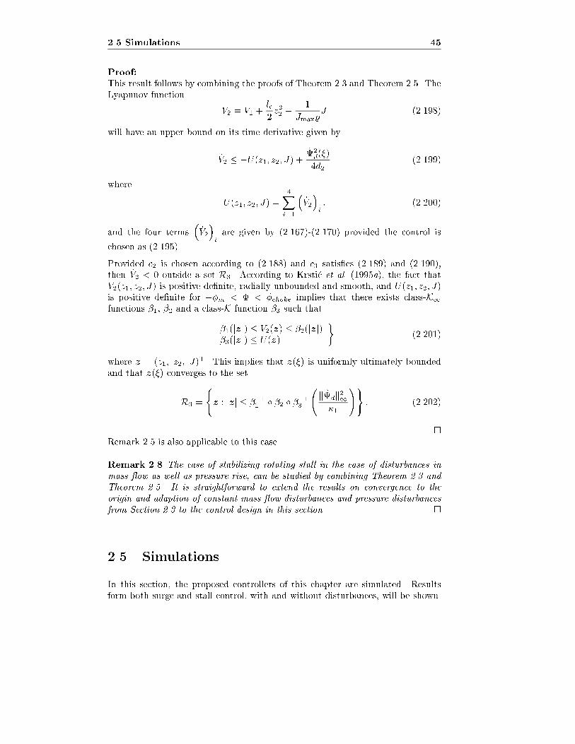
2.5 Simulations 45
Proof:
This result follows by combining the proofs of Theorem 2.3 and Theorem 2.5. TheLyapunov function
V2 = V1 +lc
2z22 +
1
Jmax%J (2.198)
will have an upper bound on its time derivative given by
_V2 � �U(z1; z2; J) + 2d(�)
4d2(2.199)
where
U(z1; z2; J) =
4Xi=1
�_V2
�i
: (2.200)
and the four terms�_V2
�i
are given by (2.167)-(2.170) provided the control is
chosen as (2.195).
Provided c2 is chosen according to (2.188) and c3 satis�es (2.189) and (2.190),then _V2 < 0 outside a set R3. According to Krsti�c et al. (1995a), the fact thatV2(z1; z2; J) is positive de�nite, radially unbounded and smooth, and U(z1; z2; J)is positive de�nite for ��m < � < �choke implies that there exists class-K1functions �1, �2 and a class-K function �3 such that
�1(jzj) � V2(z) � �2(jzj)�3(jzj) � U(z)
�(2.201)
where z = (z1; z2; J)T. This implies that z(�) is uniformly ultimately bounded
and that z(�) converges to the set
R3 =
(z : jzj � ��11 � �2 � ��13
kdk21�1
!): (2.202)
�
Remark 2.5 is also applicable to this case.
Remark 2.8 The case of stabilizing rotating stall in the case of disturbances in
mass ow as well as pressure rise, can be studied by combining Theorem 2.3 and
Theorem 2.5. It is straightforward to extend the results on convergence to the
origin and adaption of constant mass ow disturbances and pressure disturbances
from Section 2.3 to the control design in this section. �
2.5 Simulations
In this section, the proposed controllers of this chapter are simulated. Resultsform both surge and stall control, with and without disturbances, will be shown.
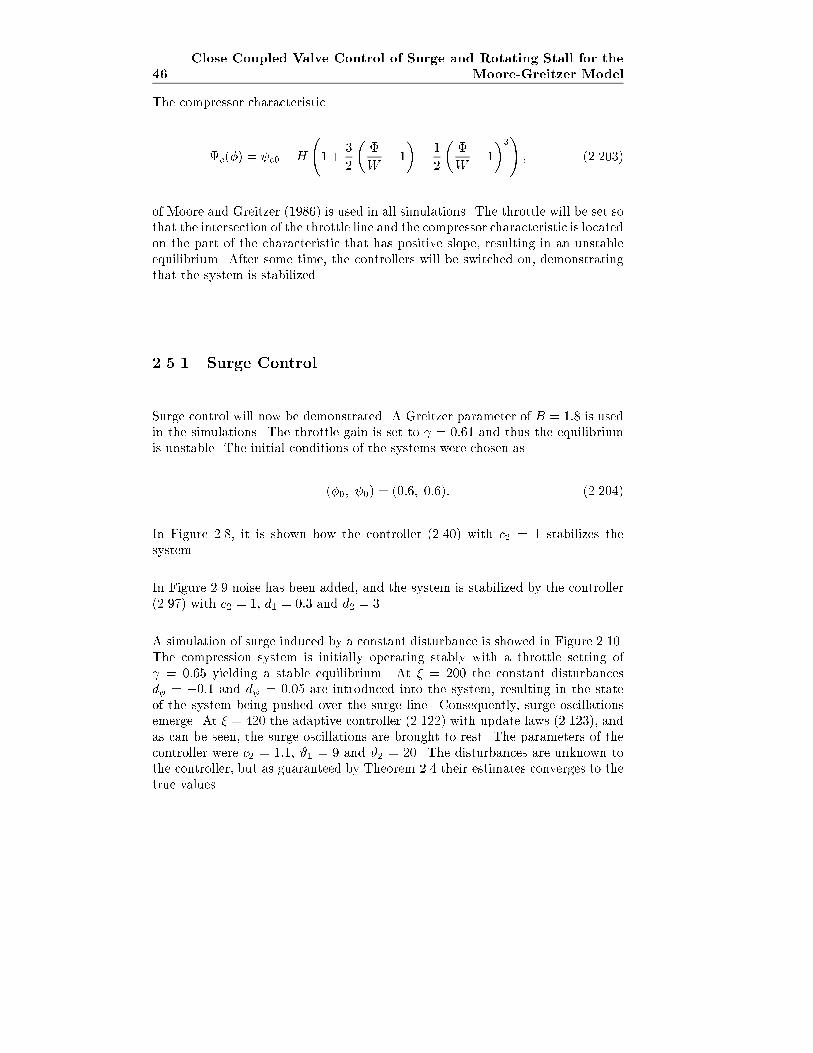
46
Close Coupled Valve Control of Surge and Rotating Stall for the
Moore-Greitzer Model
The compressor characteristic
c(�) = c0 +H
1 +
3
2
��
W� 1
�� 1
2
��
W� 1
�3!; (2.203)
of Moore and Greitzer (1986) is used in all simulations. The throttle will be set sothat the intersection of the throttle line and the compressor characteristic is locatedon the part of the characteristic that has positive slope, resulting in an unstableequilibrium. After some time, the controllers will be switched on, demonstratingthat the system is stabilized.
2.5.1 Surge Control
Surge control will now be demonstrated. A Greitzer parameter of B = 1:8 is usedin the simulations. The throttle gain is set to = 0:61 and thus the equilibriumis unstable. The initial conditions of the systems were chosen as
(�0; 0) = (0:6; 0:6): (2.204)
In Figure 2.8, it is shown how the controller (2.40) with c2 = 1 stabilizes thesystem.
In Figure 2.9 noise has been added, and the system is stabilized by the controller(2.97) with c2 = 1, d1 = 0:3 and d2 = 3.
A simulation of surge induced by a constant disturbance is showed in Figure 2.10.The compression system is initially operating stably with a throttle setting of = 0:65 yielding a stable equilibrium. At � = 200 the constant disturbancesd� = �0:1 and d = 0:05 are introduced into the system, resulting in the stateof the system being pushed over the surge line. Consequently, surge oscillationsemerge. At � = 420 the adaptive controller (2.122) with update laws (2.123), andas can be seen, the surge oscillations are brought to rest. The parameters of thecontroller were c2 = 1:1, #1 = 9 and #2 = 20. The disturbances are unknown tothe controller, but as guaranteed by Theorem 2.4 their estimates converges to thetrue values.
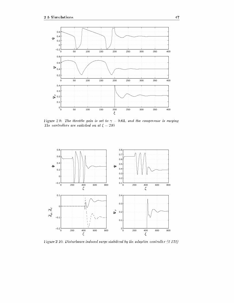
2.5 Simulations 47
0 50 100 150 200 250 300 350 400−0.2
0
0.2
0.4
0.6
0 50 100 150 200 250 300 350 400
0.2
0.4
0.6
0.8
0 50 100 150 200 250 300 350 4000
0.1
0.2
0.3
0.4
�
�
v
Figure 2.8: The throttle gain is set to = 0:61, and the compressor is surging.
The controllers are switched on at � = 200.
0 200 400 600 800−0.2
0
0.2
0.4
0.6
0.8
0 200 400 600 8000.1
0.2
0.3
0.4
0.5
0.6
0.7
0.8
0 200 400 600 800−0.2
−0.1
0
0.1
0 200 400 600 8000
0.1
0.2
0.3
0.4
��
��
�
d�;d
v
Figure 2.10: Disturbance induced surge stabilized by the adaptive controller (2.122).
48
Close Coupled Valve Control of Surge and Rotating Stall for the
Moore-Greitzer Model
0 50 100 150 200 250 300 350 400−0.2
0
0.2
0.4
0.6
0 50 100 150 200 250 300 350 4000.2
0.4
0.6
0.8
0 50 100 150 200 250 300 350 4000
0.1
0.2
�
�
�
�
v
Figure 2.9: Same situation as in Figure 2.8. However, here disturbances are taken
into account. The pressure and the mass ow disturbances are both white noise
varying between �0:05.
2.5.2 Rotating Stall Control
In this section some simulation results of the proposed controllers for rotatingstall are presented. In Figure 2.11 the response of system (2.34) with controller(2.165) is shown. The throttle gain is set at T = 0:61, resulting in an unstableequilibrium for the unactuated system. The initial conditions of the systems werechosen as
(�0 ; 0; J0) = (0:6; 0:6; 0:05): (2.205)
The B-parameter is set to B = 0:5 for all the rotating stall simulations. Thus, thecompressor enter rotating stall, and J increases until Je is reached. At � = 100the controller is switched on, and J decreases until J = 0 is reached. As discussedat the end of Section 2.4.1, the controller gains are chosen as c3 = 0 and c2 = 1.The simulation results are also plotted together with the compressor characteristicand the in-stall characteristic in Figure 2.12. As the compressor is stabilized itis seen that the pressure loss associated with the CCV is slightly less than thatassociated with operating in rotating stall, which would have been the case if e.g.the throttle control scheme of Krsti�c et al. (1995b) had been used.
The e�ect of pressure disturbances is shown in Figure 2.13. The B-parameter isB = 0:5 and the compressor stalls. The pressure disturbance is white noise ofamplitude 0:1. Throttle setting and initial conditions were left unchanged. Thecontrol law (2.195) with parameters c2 = 1 and d2 = 0:1 is switched on at � = 100,bringing the compressor out of rotating stall, and damping the disturbances.
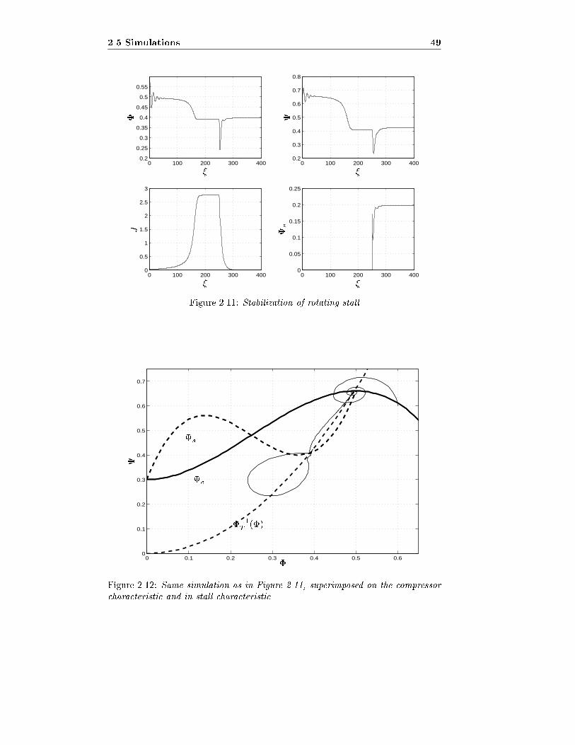
2.5 Simulations 49
0 100 200 300 4000.2
0.25
0.3
0.35
0.4
0.45
0.5
0.55
0 100 200 300 4000.2
0.3
0.4
0.5
0.6
0.7
0.8
0 100 200 300 4000
0.5
1
1.5
2
2.5
3
0 100 200 300 4000
0.05
0.1
0.15
0.2
0.25
��
��
�
J v
Figure 2.11: Stabilization of rotating stall
0 0.1 0.2 0.3 0.4 0.5 0.60
0.1
0.2
0.3
0.4
0.5
0.6
0.7
�
ss
cc
��1T(�)
Figure 2.12: Same simulation as in Figure 2.11, superimposed on the compressor
characteristic and in-stall characteristic
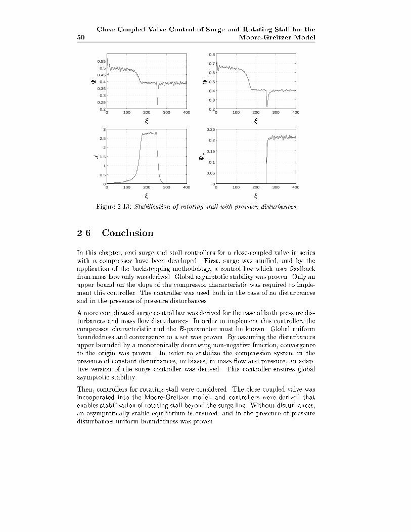
50
Close Coupled Valve Control of Surge and Rotating Stall for the
Moore-Greitzer Model
0 100 200 300 4000.2
0.25
0.3
0.35
0.4
0.45
0.5
0.55
0 100 200 300 4000.2
0.3
0.4
0.5
0.6
0.7
0.8
0 100 200 300 4000
0.5
1
1.5
2
2.5
3
0 100 200 300 4000
0.05
0.1
0.15
0.2
0.25
��
��
�
J v
Figure 2.13: Stabilization of rotating stall with pressure disturbances
2.6 Conclusion
In this chapter, anti surge and stall controllers for a close-coupled valve in serieswith a compressor have been developed. First, surge was studied, and by theapplication of the backstepping methodology, a control law which uses feedbackfrom mass ow only was derived. Global asymptotic stability was proven. Only anupper bound on the slope of the compressor characteristic was required to imple-ment this controller. The controller was used both in the case of no disturbancesand in the presence of pressure disturbances.
A more complicated surge control law was derived for the case of both pressure dis-turbances and mass ow disturbances. In order to implement this controller, thecompressor characteristic and the B-parameter must be known. Global uniformboundedness and convergence to a set was proven. By assuming the disturbancesupper bounded by a monotonically decreasing non-negative function, convergenceto the origin was proven. In order to stabilize the compression system in thepresence of constant disturbances, or biases, in mass ow and pressure, an adap-tive version of the surge controller was derived. This controller ensures globalasymptotic stability.
Then, controllers for rotating stall were considered. The close coupled valve wasincooperated into the Moore-Greitzer model, and controllers were derived thatenables stabilization of rotating stall beyond the surge line. Without disturbances,an asymptotically stable equilibrium is ensured, and in the presence of pressuredisturbances uniform boundedness was proven.
Chapter 3
Passivity Based Surge
Control
3.1 Introduction
In this chapter passivity will be used to derive a surge controller for a compressionsystem when time varying disturbances are considered in both pressure as well asmass ow.
Passivity and input/output methods have been used in many control applicationssuch as mechanical systems in general, electrical machines, marine vehicles and soon. To the authors best knowledge this is the �rst attempt to apply this methodto the compressor surge control problem.
3.1.1 Motivation
In the previous chapter, backstepping was employed to derive a stabilizing controllaw when time varying disturbances were taken into account. The control lawresulting from this approach was
u = c2z2 � k3��3 + 3�z22
�� k2�2 � k1� (3.1)
+d1
4B2
���T (z1) + �
�+ d2z2
�1 +
d214B2
�:
Of particular interest here, will be the use of input/output methods to designcontrollers with disturbance rejection capabilities. This is motivated by the factthat the surge controller (3.1) seems unnecessary complicated.
52 Passivity Based Surge Control
3.1.2 Notation
A brief introduction to passivity and L2 is given here. For a comprehensivetreatment of these concepts, consult van der Schaft (1996), from which the no-tation is taken. The signal space L2 consists, somewhat simpli�ed, of all functionsf : IIR+ ! IIR that satisfy Z 1
0
jf(�)j2d� <1: (3.2)
The truncation of f to [0; T ] is de�ned as
fT (�) =
�f(�) ; 0 � � < T
0 ; � � T; (3.3)
and the set L2e, the extension of L2, consists of all functions f such that fT 2 L2.A mapping G : u 7! y with input u 2 L2e and output y 2 L2e is said to be passiveif there exists a constant � so that
ZT
0
u(�)y(�)d� � � (3.4)
for all u 2 L2e and all T � 0. The inner product on L2e is
hu; yiT=
ZT
0
u(�)y(�)d�; (3.5)
and the truncated norm is
kuk2T= hu; ui
T: (3.6)
A concept that will be used in this chapter is that of strict output passivity. Themapping G : u 7! y is strict output passive if 9 � > 0 and 9 � such that
hy; ui = hGu; ui � �kGuk2T+ � 8u 2 L2e; 8T � 0: (3.7)
3.2 Model
A compression system consisting of a compressor, axial or centrifugal, in series witha close-coupled valve, a plenum volume and a throttle is studied, consult �gure 2.3.The system is presented in section 2.2.4, and repeated here for convenience:
_ =
1
4B2lc(�� �T ( )) (3.8)
_� =
1
lc(c(�)� u� );
where u = v, and the equivalent compressor characteristic is e = c� v. Thenotation _x is to be understood as di�erentiation with respect to nondimensionaltime � = Ut
Ras in the previous chapter.
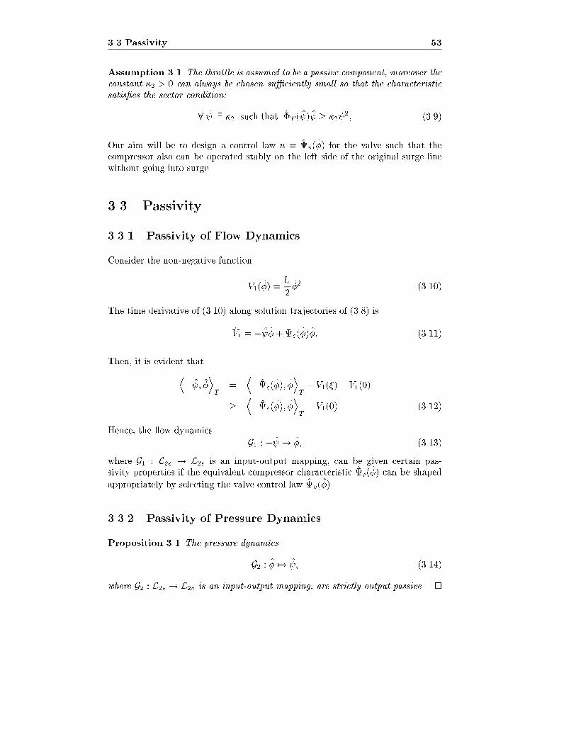
3.3 Passivity 53
Assumption 3.1 The throttle is assumed to be a passive component, moreover the
constant �2 > 0 can always be chosen su�ciently small so that the characteristic
satis�es the sector condition:
8 9 �2 such that �T ( ) � �2 2; (3.9)
Our aim will be to design a control law u = v(�) for the valve such that thecompressor also can be operated stably on the left side of the original surge linewithout going into surge.
3.3 Passivity
3.3.1 Passivity of Flow Dynamics
Consider the non-negative function
V1(�) =lc
2�2 (3.10)
The time derivative of (3.10) along solution trajectories of (3.8) is
_V1 = � �+e(�)�: (3.11)
Then, it is evident thatD� ; �
ET
=D�e(�); �
ET
+ V1(�)� V1(0)
�D�e(�); �
ET
� V1(0) (3.12)
Hence, the ow dynamics
G1 : � 7! �; (3.13)
where G1 : L2e ! L2e is an input-output mapping, can be given certain pas-sivity properties if the equivalent compressor characteristic e(�) can be shaped
appropriately by selecting the valve control law v(�).
3.3.2 Passivity of Pressure Dynamics
Proposition 3.1 The pressure dynamics
G2 : � 7! ; (3.14)
where G2 : L2e ! L2e is an input-output mapping, are strictly output passive. �
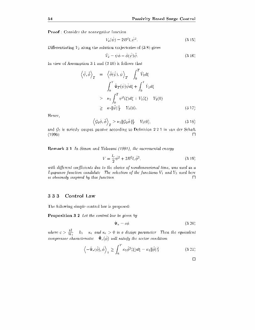
54 Passivity Based Surge Control
Proof : Consider the nonnegative function
V2( ) = 2B2lc 2: (3.15)
Di�erentiating V2 along the solution trajectories of (3.8) gives
_V2 = �� �( ) : (3.16)
In view of Assumption 3.1 and (3.16) it follows thatD ; �
ET
=D�( );
ET
+
ZT
0
_V2d�
=
ZT
0
�T ( ) d� +
ZT
0
_V2d�
� �2
ZT
0
2(�)d� + V2(�) � V2(0)
� �2k k2T � V2(0): (3.17)
Hence, DG2�; �
ET
� �2kG2�k2T � V2(0); (3.18)
and G2 is strictly output passive according to De�nition 2.2.1 in van der Schaft(1996). �
Remark 3.1 In Simon and Valavani (1991), the incremental energy
V =lc
2 2 + 2B2lc�
2; (3.19)
with di�erent coe�cients due to the choice of nondimensional time, was used as a
Lyapunov function candidate. The selection of the functions V1 and V2 used here
is obviously inspired by this function. �
3.3.3 Control Law
The following simple control law is proposed:
Proposition 3.2 Let the control law be given by
v = c� (3.20)
where c >k22
4k3� k1 + �1 and �1 > 0 is a design parameter. Then the equivalent
compressor characteristic �e(�) will satisfy the sector conditionD�e(�); �
ET
�ZT
0
�1�2(�)d� = �1k�k2T (3.21)
�
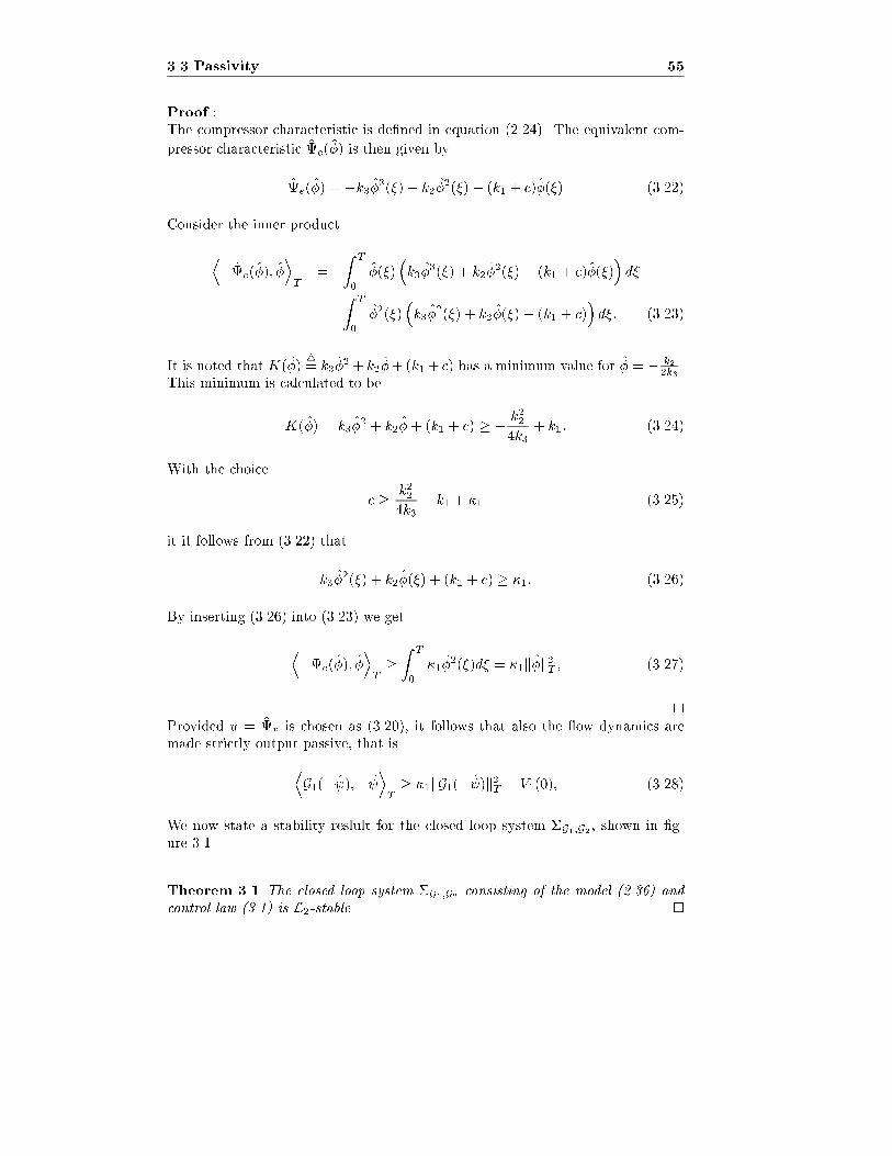
3.3 Passivity 55
Proof :The compressor characteristic is de�ned in equation (2.24). The equivalent com-
pressor characteristic e(�) is then given by
e(�) = �k3�3(�)� k2�2(�) � (k1 + c)�(�) (3.22)
Consider the inner product
D�e(�); �
ET
=
ZT
0
�(�)�k3�
3(�) + k2�2(�) + (k1 + c)�(�)
�d�
=
ZT
0
�2(�)�k3�
2(�) + k2�(�) + (k1 + c)�d�: (3.23)
It is noted that K(�)4= k3�
2 + k2�+(k1 + c) has a minimum value for � = � k2
2k3.
This minimum is calculated to be
K(�) = k3�2 + k2�+ (k1 + c) � � k22
4k3+ k1: (3.24)
With the choice
c � k224k3
� k1 + �1 (3.25)
it it follows from (3.22) that
k3�2(�) + k2�(�) + (k1 + c) � �1: (3.26)
By inserting (3.26) into (3.23) we get
D�e(�); �
ET
�ZT
0
�1�2(�)d� = �1k�k2T ; (3.27)
�
Provided u = v is chosen as (3.20), it follows that also the ow dynamics aremade strictly output passive, that is
DG1(� );�
ET
� �1kG1(� )k2T � V1(0); (3.28)
We now state a stability reslult for the closed loop system �G1;G2 , shown in �g-ure 3.1.
Theorem 3.1 The closed loop system �G1;G2 consisting of the model (2.36) and
control law (3.1) is L2-stable. �
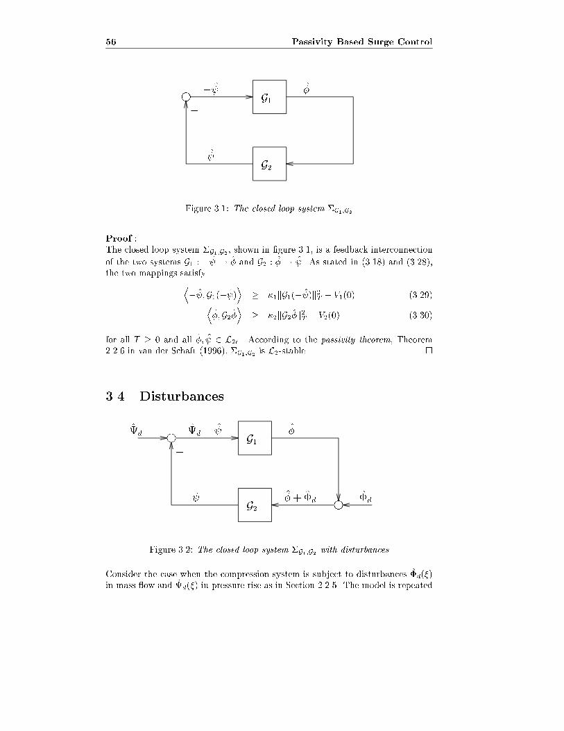
56 Passivity Based Surge Control
h �
�
�
G1
G2
Figure 3.1: The closed loop system �G1;G2
Proof :The closed loop system �G1;G2 , shown in �gure 3.1, is a feedback interconnection
of the two systems G1 : � 7! � and G2 : � 7! . As stated in (3.18) and (3.28),the two mappings satisfyD
� ;G1(� )E
� �1kG1(� )k2T � V1(0) (3.29)D�;G2�
E� �2kG2�k2T � V2(0) (3.30)
for all T � 0 and all �; 2 L2e. According to the passivity theorem, Theorem2.2.6 in van der Schaft (1996), �G1;G2 is L2-stable. �
3.4 Disturbances
h
h
�
�
G1
G2
d �
�d�+ �d
d
Figure 3.2: The closed loop system �G1;G2 with disturbances
Consider the case when the compression system is subject to disturbances �d(�)in mass ow and d(�) in pressure rise as in Section 2.2.5. The model is repeated
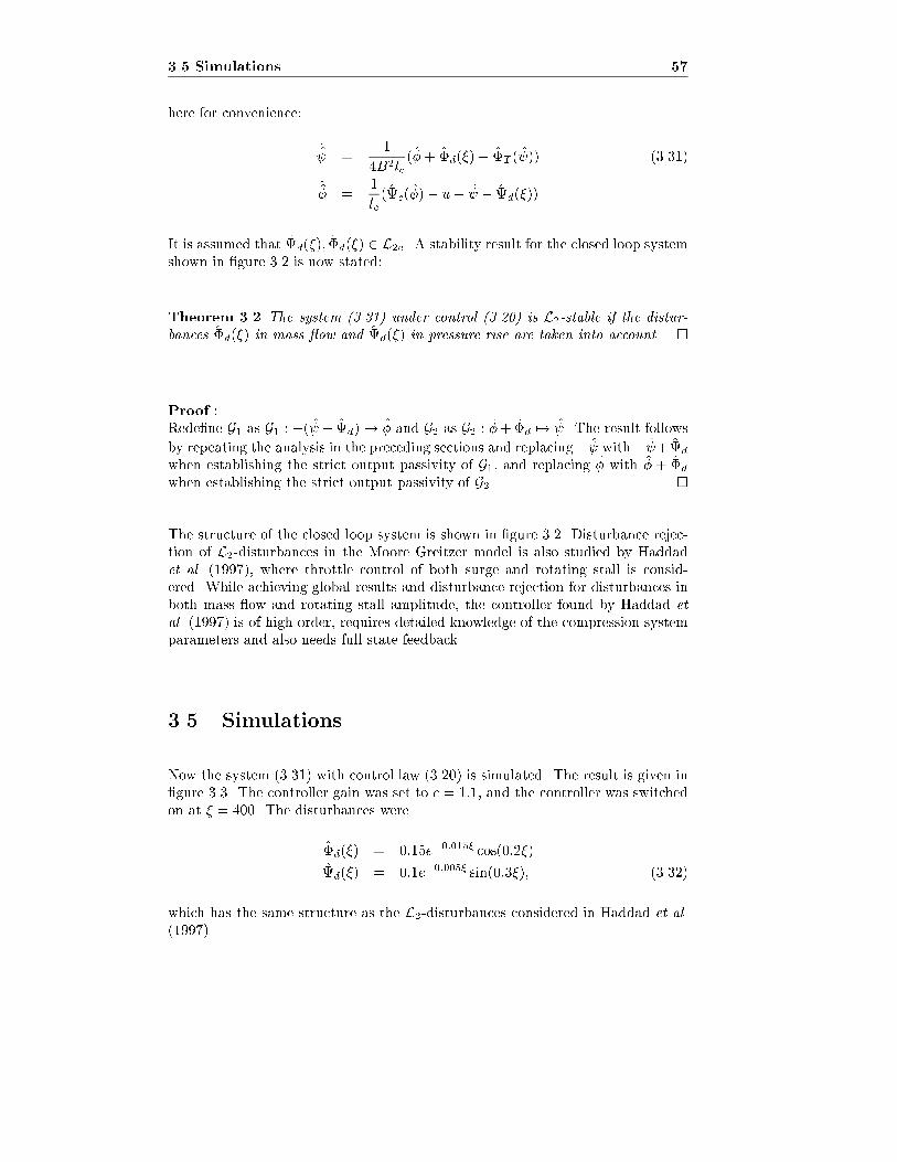
3.5 Simulations 57
here for convenience:
_ =
1
4B2lc(�+ �d(�)� �T ( )) (3.31)
_� =
1
lc(c(�)� u� � d(�))
It is assumed that d(�); �d(�) 2 L2e. A stability result for the closed loop systemshown in �gure 3.2 is now stated:
Theorem 3.2 The system (3.31) under control (3.20) is L2-stable if the distur-
bances �d(�) in mass ow and d(�) in pressure rise are taken into account. �
Proof :Rede�ne G1 as G1 : �( � d) 7! � and G2 as G2 : �+�d 7! . The result follows
by repeating the analysis in the preceding sections and replacing � with � +dwhen establishing the strict output passivity of G1, and replacing � with � + �dwhen establishing the strict output passivity of G2. �
The structure of the closed loop system is shown in �gure 3.2. Disturbance rejec-tion of L2-disturbances in the Moore Greitzer model is also studied by Haddadet al. (1997), where throttle control of both surge and rotating stall is consid-ered. While achieving global results and disturbance rejection for disturbances inboth mass ow and rotating stall amplitude, the controller found by Haddad et
al. (1997) is of high order, requires detailed knowledge of the compression systemparameters and also needs full state feedback.
3.5 Simulations
Now the system (3.31) with control law (3.20) is simulated. The result is given in�gure 3.3. The controller gain was set to c = 1:1, and the controller was switchedon at � = 400. The disturbances were
�d(�) = 0:15e�0:015� cos(0:2�)
d(�) = 0:1e�0:005� sin(0:3�); (3.32)
which has the same structure as the L2-disturbances considered in Haddad et al.
(1997).
58 Passivity Based Surge Control
0 100 200 300 400 500 600 700 800−0.2
0
0.2
0.4
0.6
0 100 200 300 400 500 600 700 8000.2
0.4
0.6
0.8
400 410 420 430 4400
0.1
0.2
0.3
0.4
0 200 400 600 8000
0.1
0.2
0.3
0.4
��
�
�
�
v
v
Figure 3.3: Comparison of closed loop response with passivity based (solid lines)
and backstepping based (dashed lines) controllers. The controllers were switched
on at � = 400.
Also plotted in Figure 3.3 is the response of the controller (3.1), simulated withthe same disturbances. The parameters for (3.1) were chosen as c2 = 1, d1 = 0:3,d2 = 0:1. The two set of responses are almost indistinguishable, but in the lowerleft plot there is a blown up plot of the CCV pressure drop, and as can be seen thereis a small di�erence. Figure 3.3 also illustrates the result of Corollary 2.2, wherethe controller (3.1) guarantees convergence to the equilibrium in the presence ofdisturbances upper bounded by a monotonically decreasing non-negative function.The small di�erence in control action is due to the low damping (di) chosen for(3.1), but with the current disturbances that is all that was needed.
One advantage of the backstepping controller (3.1) compared to the passivity based(3.20) is that (3.1) ensures convergence to a set when the disturbances are not inL2, whereas the approach in this chapter demands that they are in L2.
3.6 Concluding Remarks
In this chapter the passivity properties of the Greitzer model was used to derivea surge control law for a close coupled valve. The results in this chapter, whennot taking disturbances into account, are similar to the results in section 2.3.1.However, using input/output theory and passivity it was possible to show that
the proportional controller u = c� yielded an L2-stable system in the presence of
3.6 Concluding Remarks 59
both mass ow disturbances as well as pressure disturbances. Compared to themore complicated controller (3.1) the advantages of the input/output approachover the Lyapunov based approach of backstepping, in this particular case, shouldbe evident.
However, it is believed that the simple controller u = c� also could have beenderived using backstepping, but with considerable more involved algebraic manip-ulations, and possibly a new choice of Lyapunov function candidate.
It is straightforward to show that the stability result is still valid if the controllaw (3.20) is changed as long as the sector condition (3.21) hold. Thus, a moresophisticated controller could be used in order to e.g. minimize the steady statepressure drop over the CCV or improve transient performance, and still stabilitycould be shown.
When comparing with the results on rotating stall control in Haddad et al. (1997),the passivity based method used here shows promise for developing a simple, loworder, partial state feedback controller when rotating stall is also taken into ac-count, and still achieving disturbance rejection. This is an interesting open prob-lem.

60 Passivity Based Surge Control
Chapter 4
A Moore-Greitzer Type
Model for Axial
Compressors with
Non-constant Speed
4.1 Introduction
In this chapter we propose an extension to the Moore-Greitzer model. Non-constant rotational speed of the compressor is taken into account. The conse-quence of this is that the new model includes the B-parameter as a state. Higherharmonics of rotating stall will also be included in the model.
In the original work of Moore and Greitzer, the compressor speed is assumedconstant. Greitzer and Moore (1986) concluded that low values of Greitzer's B-parameter B lead to rotating stall, while high value of B leads to surge. Highand low in this context is dependent on the design parameters of the compressorat hand, as Day (1994) points out. There exists a Bcritical for which higher B-values will lead to surge and lower B-values will lead to rotating stall. However thisBcritical is di�erent for each compressor. As B is proportional to the angular speedof the machine, it is of major concern for stall/surge controller design to includethe spool dynamics in a stall/surge-model, in order to investigate the in uence oftime varying speed on the stall/surge transients.
A model for centrifugal compressors with non-constant speed was presented byFink et al. (1992). In Gravdahl and Egeland (1997g) a similar model was derived,and surge and speed control was investigated. However, both the models of Finket al. (1992) and Gravdahl and Egeland (1997g) were developed for centrifugalmachines, and do not include rotating stall as a state.
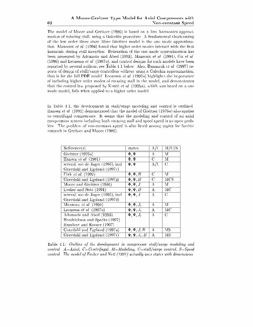
62
A Moore-Greitzer Type Model for Axial Compressors with
Non-constant Speed
The model of Moore and Greitzer (1986) is based on a �rst harmonics approxi-mation of rotating stall, using a Galerkin procedure. A fundamental shortcomingof the low order three state More Greitzer model is the one mode approxima-tion. Mansoux et al. (1994) found that higher order modes interact with the �rstharmonic during stall inception. Relaxation of the one mode approximation hasbeen presented by Adomatis and Abed (1993), Mansoux et al. (1994), Gu et al.
(1996) and Leonessa et al. (1997a), and control designs for such models have beenreported by several authors, see Table 4.1 below. Also, Banaszuk et al. (1997) re-ports of design of stall/surge controllers without using a Galerkin approximation,that is for the full PDE model. Leonessa et al. (1997a) highlights the importanceof including higher order modes of rotating stall in the model, and demonstratesthat the control law proposed by Krsti�c et al. (1995a), which was based on a onemode model, fails when applied to a higher order model.
In Table 4.1, the development in stall/surge modeling and control is outlined.Hansen et al. (1981) demonstrated that the model of Greitzer (1976a) also appliesto centrifugal compressors. It seems that the modeling and control of an axialcompression system including both rotating stall and spool speed is an open prob-lem. The problem of non-constant speed is also listed among topics for furtherresearch in Greitzer and Moore (1986).
Reference(s) states A/C M/C/S
Greitzer (1976a) �; A M
Hansen et al. (1981) �; C M
several, see de Jager (1995), incl. �; A/C CGravdahl and Egeland (1997c)
Fink et al. (1992) �;; B C M
Gravdahl and Egeland (1997g) �;; B C MCS
Moore and Greitzer (1986) �;; J A M
Eveker and Nett (1991) �;; B A MC
several, see de Jager (1995), incl. �;; J A CGravdahl and Egeland (1997d)
Mansoux et al. (1994) �;; Ji A M
Leonessa et al. (1997a) �;; Ji A MC
Adomatis and Abed (1993) �;; Ji A CHendrickson and Sparks (1997)Humbert and Krener (1997)
Gravdahl and Egeland (1997a) �;; J; B A MS
Gravdahl and Egeland (1997e) �;; Ji; B A MS
Table 4.1: Outline of the development in compressor stall/surge modeling and
control. A=Axial, C=Centrifugal, M=Modeling, C=stall/surge control, S=Speed
control. The model of Eveker and Nett (1991) actually uses states with dimensions.
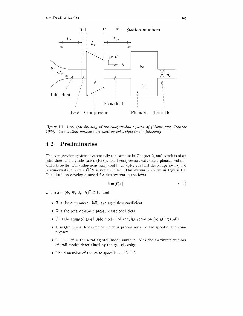
4.2 Preliminaries 63
HHHHH
�����
AAA���
Station numbersE10
LI
Lc
LE
�
�
pTCx
ps
pT
Vp
ThrottlePlenum
Exit duct
CompressorIGV
Inlet duct
Figure 4.1: Principal drawing of the compression system of (Moore and Greitzer
1986). The station numbers are used as subscripts in the following.
4.2 Preliminaries
The compression system is essentially the same as in Chapter 2, and consists of aninlet duct, inlet guide vanes (IGV), axial compressor, exit duct, plenum volumeand a throttle. The di�erences compared to Chapter 2 is that the compressor speedis non-constant, and a CCV is not included. The system is shown in Figure 4.1.Our aim is to develop a model for this system in the form
_z = f(z); (4.1)
where z = (�; ; Ji; B)T 2 IIRq and
� � is the circumferentially averaged ow coe�cient
� is the total-to-static pressure rise coe�cient
� Ji is the squared amplitude mode i of angular variation (rotating stall)
� B is Greitzer's B-parameter which is proportional to the speed of the com-pressor.
� i = 1 : : :N is the rotating stall mode number. N is the maximum numberof stall modes determined by the gas viscosity.
� The dimension of the state space is q = N + 3:
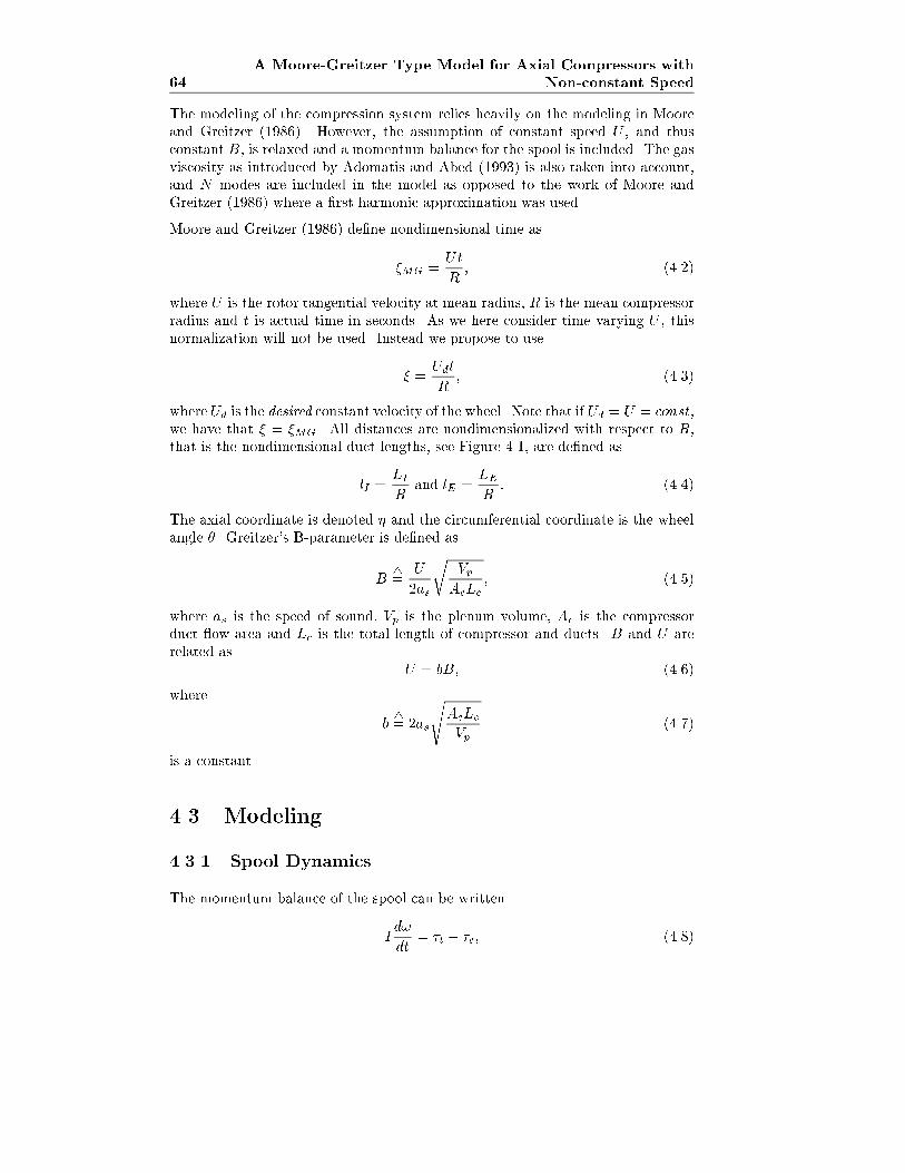
64
A Moore-Greitzer Type Model for Axial Compressors with
Non-constant Speed
The modeling of the compression system relies heavily on the modeling in Mooreand Greitzer (1986). However, the assumption of constant speed U , and thusconstant B, is relaxed and a momentum balance for the spool is included. The gasviscosity as introduced by Adomatis and Abed (1993) is also taken into account,and N modes are included in the model as opposed to the work of Moore andGreitzer (1986) where a �rst harmonic approximation was used.
Moore and Greitzer (1986) de�ne nondimensional time as
�MG =Ut
R; (4.2)
where U is the rotor tangential velocity at mean radius, R is the mean compressorradius and t is actual time in seconds. As we here consider time varying U , thisnormalization will not be used. Instead we propose to use
� =Udt
R; (4.3)
where Ud is the desired constant velocity of the wheel. Note that if Ud = U = const,we have that � = �MG. All distances are nondimensionalized with respect to R,that is the nondimensional duct lengths, see Figure 4.1, are de�ned as
lI =LI
Rand lE =
LE
R: (4.4)
The axial coordinate is denoted � and the circumferential coordinate is the wheelangle �. Greitzer's B-parameter is de�ned as
B4=
U
2as
rVp
AcLc; (4.5)
where as is the speed of sound, Vp is the plenum volume, Ac is the compressorduct ow area and Lc is the total length of compressor and ducts. B and U arerelated as
U = bB; (4.6)
where
b4= 2as
sAcLc
Vp(4.7)
is a constant.
4.3 Modeling
4.3.1 Spool Dynamics
The momentum balance of the spool can be written
Id!
dt= �t � �c; (4.8)
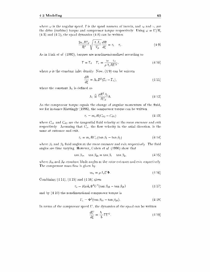
4.3 Modeling 65
where ! is the angular speed, I is the spool moment of inertia, and �t and �c arethe drive (turbine) torque and compressor torque respectively. Using ! = U=R,(4.3) and (4.5), the spool dynamics (4.8) can be written
2asIUdR2
sAcLc
Vp
dB
d�= �t � �c: (4.9)
As in Fink et al. (1992), torques are nondimensionalized according to
� = �t � �c =�t � �c
�AcRU2; (4.10)
where � is the constant inlet density. Now, (4.9) can be written
dB
d�= �1B
2(�t � �c); (4.11)
where the constant �1 is de�ned as
�14=�R3Ac
IUdb: (4.12)
As the compressor torque equals the change of angular momentum of the uid,see for instance Mattingly (1996), the compressor torque can be written
�c = mcR(C�2 � C�1) (4.13)
where C�1 and C�2 are the tangential uid velocity at the rotor entrance and exitrespectively. Assuming that Cx, the ow velocity in the axial direction, is thesame at entrance and exit,
�c = mcRCx(tan�1 � tan�2) (4.14)
where �1 and �2 uid angles at the rotor entrance and exit respectively. The uidangles are time varying. However, Cohen et al. (1996) show that
tan�1b � tan�2b = tan�1 � tan�2; (4.15)
where �1b and �b2 constant blade angles at the rotor entrance and exit respectively.The compressor mass ow is given by
mc = �AcU�: (4.16)
Combining (4.14), (4.15) and (4.16) gives
�c = R�Ac�2U2(tan�1b � tan�2b) (4.17)
and by (4.10) the nondimensional compressor torque is
�c = �2(tan�1b � tan�2b): (4.18)
In terms of the compressor speed U , the dynamics of the spool can be written
dU
d�=
�1b�U2: (4.19)
66
A Moore-Greitzer Type Model for Axial Compressors with
Non-constant Speed
4.3.2 Compressor
Moore (1984a) gives the pressure rise over a single blade row as
pE � p112�U2
= F (�) � �d�
dt; (4.20)
where
� =Cx
U(4.21)
is the local axial ow coe�cient, F (�) is the pressure rise coe�cient in the bladepassage, Cx is the velocity component along the x-axis, and � is a coe�cient ofpressure rise lag. According to Moore and Greitzer (1986), d�
dtcan be calculated
asd�
dt=
�@�
@t
�rotor
+
�@�
@t
�stator
: (4.22)
Using (4.3) it is seen that�@�
@t
�rotor
=@�
@�
@�
@t+@�
@�
@�
@t
=Ud
R
@�
@�+@�
@�
U(t)
R(4.23)�
@�
@t
�stator
=Ud
R
@�
@�; (4.24)
where the unsteadiness of the ow through the stator passage re ects the acceler-ations associated with transients e�ects. For the rotor there is also unsteadinessdue to the rotor blades moving with velocity U(t) through a circumferentiallynonuniform ow. Considering a compressor of Ns stages, we get
pE � p112�U2
= NsF (�)� 1
2a
�2@�
@�+U
Ud
@�
@�
�; (4.25)
where
a4=
R
Ns�Ud(4.26)
is a constant. Note that if U(�) = const and Ud � U such that � = �MG, equation(4.25) is reduced to equation (5) in Moore and Greitzer (1986). It is noted thatthe ow coe�cient � can depend on both � and �, even though the atmosphericstagnation pressure pT is constant. The average of � around the wheel is de�nedas
1
2�
Z 2�
0
�(�; �)d�4= �(�): (4.27)
Further� = �(�) + g(�; �) and h = h(�; �); (4.28)
where h is a circumferential coe�cient. As no circulation occurs in the entranceduct it is clear that the averages of g and h vanish:Z 2�
0
g(�; �)d� =
Z 2�
0
h(�; �)d� = 0: (4.29)
4.3 Modeling 67
4.3.3 Entrance Duct and Guide Vanes
The fact that the rotational speed of the wheel now is assumed time varying doesnot change the conditions upstream of the compressor. Therefore the equationsstated in Moore and Greitzer (1986) are still valid, and will be presented here.The pressure di�erence over the IGVs, where the ow is axial, can be written
p1 � p0
�U2=
1
2KGh
2; (4.30)
where 0 < KG � 1 is the entrance recovery coe�cient. If the IGVs are losslessKG = 1. Upstream of the IGV irrotational ow is assumed so that a (unsteady)velocity potential ~� exists. The gradient of ~� gives axial and circumferential ve-locity coe�cients everywhere in the entrance duct. At the IGV entrance point(denoted by subscript '0') we have
(~��)0 = �(�) + g(�; �) and (~��)0 = h(�; �); (4.31)
where partial di�erentiation with respect to � and � is denoted by subscripts.Bernoulli's equation for unsteady, frictionless and incompressible ow will be usedto calculate the pressure drop in the entrance duct. As in Moore and Greitzer(1986) and White (1986), this can be written
pT � p0
�U2=
1
2(�2 + h2) + (~��)0; (4.32)
where the term (~��)0 is due to unsteadiness in � and g. A straight inlet duct ofnondimensional length lI is considered, and the velocity potential can be written
~� = (� + lI)�(�) + ~�0(�; �); (4.33)
where ~�0 is a disturbance velocity potential such that
~�0����=�lI
= 0 ; (~�0�)0 = g(�; �) and (~�0
�)0 = h(�; �): (4.34)
Equation (4.32) can now be written
pT � p0
�U2=
1
2(�2 + h2) + lI
d�
d�+ (~�0
�)0: (4.35)
4.3.4 Exit Duct and Guide Vanes
Downstream of the compressor the ow is complicated and rotational. As in Mooreand Greitzer (1986), the pressure p in the exit duct is assumed to di�er only slightlyfrom the static plenum pressure ps(�), such that the pressure coe�cient P satis�esLaplace's equation.
P4=ps(�) � p
�U2; r2P = 0: (4.36)
68
A Moore-Greitzer Type Model for Axial Compressors with
Non-constant Speed
The axial Euler equation, see for instance White (1986), is used to �nd the pressuredrop across the exit duct. The Euler equation is the inviscid form of the di�erentialequation of linear momentum. If integrated along a streamline of the ow, theEuler equation will yield the frictionless Bernoulli equation. The Euler equationin the x-coordinate, neglecting gravity, can be written as
� dpdx
= �dCx
dt: (4.37)
Employing the chosen nondimensionalization of time and distance,
d
dt=Ud
R
d
d�and
d
dx=
1
R
d
d�; (4.38)
we get
dpE
dx= ��U2 1
R(P�)E (4.39)
dCx
dt=
Ud
R
d
d�
n(~��)0U
o: (4.40)
Inserting (4.39) and (4.40) in (4.37) we get the following expression for the axialEuler equation, evaluated at E, where time varying U has been taken into account
(P�)E =Ud
U2
d
d�
n(~��)0U
o
=Ud
U2
�(~���)0U + (~��)0
dU
d�
�: (4.41)
From (4.31) we have(~���)0 = ��(�) + (~�0
��)0: (4.42)
Inserting (4.31) and (4.42) into (4.41) we get
(P�)E =Ud
U
�d�
d�+ (~�0
��)0
�+Ud
U2
dU
d�
��(�) + (~�0
�)0
�: (4.43)
At the duct exit, � = lE , we want that p = ps, that is P = 0. Thus, whenintegrating (4.43), the constant of integration is chosen such that
P =Ud
U(�)
�(� � lE)
d�
d�� ~�0
�
�+Ud
U2
dU
d�
�(� � lE)�(�) � ~�0
�: (4.44)
Finally, we get
ps � pE
�U2= (P )E =
Ud
U(�)
��lE d�
d�� (m� 1)(~�0
�)0
�
+Ud
U2
dU
d�
��lE�(�)� (m� 1)(~�0)0
�; (4.45)
where, as in Moore (1984b) and Moore and Greitzer (1986), the compressor duct ow parameter1 m has been included. It is noted that if U(�) =const and Ud � U
such that � = �MG, equation (4.45) is reduced to equation (20) in Moore andGreitzer (1986).
1m = 1 for a very short exit duct, and m = 2 otherwise.
4.3 Modeling 69
4.3.5 Overall Pressure Balance
Using the preceding calculations, we now want to calculate the net pressure risefrom the upstream reservoir total pressure pT to the plenum static pressure ps atthe discharge of the exit duct. This is done by combining equations (4.25), (4.30),(4.35) and (4.45) according to
ps � pT
�U2= (NF (�)� 1
2�2)� (lI + lE
Ud
U+1
a)d�
d�
+
�(1�m)
Ud
U� 1
�(~�0�)0 � 1
2(1�KG)h
2
+Ud
U2
dU
d�
��lE�(�)� (m� 1)(~�0)0
�
� 1
2a
�2(~�0
��)0 +
U
Ud(~�0��)0
�; (4.46)
where
2@�
@�+@�
@�= 2
@�
@�+ 2
@g
@�+@g
@�
= 2@�
@�+ 2(~�0
��)0 + (~�0
��)0 (4.47)
has been used. By de�ning 2
(�) =ps � pT
�U2
c(�) = NF (�)� 1
2�2
lc(U) = lI + lEUd
U+
1
a
mU (U) = (1�m)Ud
U� 1; (4.48)
and assuming KG � 1, (4.46) can be written
(�) = c(�) � lc(U)d�
d�+mU (U)(~�
0�)0 (4.49)
+Ud
U2
dU
d�
��lE�(�)� (m� 1)(~�0)0
�
� 1
2a
�2(~�0
��) +
U
Ud(~�0��)� �(~�0
���)
�0
;
which, when assuming U = Ud and � = 0, reduces to equation (26) in Moore andGreitzer (1986). In (4.49) the �-term is included in order to account for viscoustransportation of momentum in the compressor. Viscosity was �rst introduced
2Notice that lc 6= LcR. As in Fink et al. (1992) Lc, used in the de�nition of B, is a constant.
See equation (4.5).
70
A Moore-Greitzer Type Model for Axial Compressors with
Non-constant Speed
into the Moore-Greitzer model by Adomatis and Abed (1993), and included inthe analysis of Gu et al. (1996) and Hendrickson and Sparks (1997). Adomatisand Abed (1993) concludes that the e�ect of viscous damping must be includedin a multi mode Moore-Greitzer model. This to ensure that the large velocitygradients associated with higher modes will be damped out. Without viscosity, allthe modes would have the same amplitude in fully developed rotating stall.
Equation (4.49) requires knowledge of the disturbance velocity potential ~�0 and itsderivatives. As ~�0 satis�es Laplace's equationr2 ~�0 = 0 it has a Fourier series. ThisFourier series has N terms, where the number N is dependent on �. According toAdomatis and Abed (1993) and Gu et al. (1996),
N =
� 1 for � = 0�nite for � > 0
(4.50)
By using (4.6), equation (4.49) can be written in terms of B, and by integrationof (4.49) over one cycle with respect to �, we get
(�) + lc(B)d�
d�+ lE
Ud��1b
�(�) =1
2�
Z 2�
0
c(�)d�; (4.51)
which is the annulus averaged momentum balance.
4.3.6 Plenum Mass Balance
The mass balance in the plenum can be written
d
d�(�pVp) = mc �mt; (4.52)
where �p is the plenum density, mc is the mass ow entering the plenum from thecompressor, and mt is the mass ow leaving through the throttle. Assuming thepressure variations in the plenum isentropic, we have
dpp
d�=a2s
Vp(mc �mt); (4.53)
which is shown in detail in Appendix B. By nondimensionalizing pressure with�U2, mass ow with �UAc, transforming to nondimensional time �, and takingaccount for (4.5), (4.53) can be written
d
d�=
�2B(���T )� 2
B
dB
d�; (4.54)
where the constant �2 is de�ned as
�24=
R
LcUdb: (4.55)
Using (4.11) we getd
d�=
�2B(���T )� 2�1�B: (4.56)
4.3 Modeling 71
The model of the compression system now consists of the torque balance for thespool (4.11), the local momentum balance (4.49), the annulus averaged momentumbalance (4.51) and the mass balance of the plenum (4.56).
The compression systems characteristics are taken fromMoore and Greitzer (1986).The usual third order polynomial steady state compressor characteristic presentedin Chapter 2 is used, and repeated here for convenience:
c(�) = c0 +H
�1 +
3
2(�
W� 1)� 1
2(�
W� 1)3
�; (4.57)
where the parameters c0, H and W are de�ned in Chapter 2.
The throttle characteristics is again taken to be
�T () = Tp: (4.58)
4.3.7 Galerkin Procedure
In order to transform the PDE (4.49) into a set of ODEs, a Galerkin approximationis employed. The disturbance velocity potential ~�0 is represented by the function(~�0)�:
( ~�0)� =
NXn=1
(�)W
nen�An(�) sin(n� � rn(�)); (4.59)
where An(�) is the amplitude of mode number n of rotating stall and rn(�); n =1 : : :N(�) are unknown phase angles. The residue Rn, for use in the Galerkinapproximation, is de�ned as
Rn4= (~�0
�)�0 � (~�0
�)0; (4.60)
and using (4.49) and (4.59), Rn can be calculated as
Rn =W
n
�dAn
d�sin �n �An
drn
d�cos �n
�(4.61)
� 1
mB(B)
�(�) + lc(B)
d�
d�+ lE
Ud��1b
��c (� +WAn(�) sin �n)
+Ud��1(m� 1)W
bnAn(�) sin �n +
W
2a
�2
�dAn
d�sin �n �An
drn
d�cos �n
�
+Un
UdAn(�) cos �n + �n2An(�) sin �n
��;
where
�n4= n� � rn(�): (4.62)
The Galerkin approximation is calculated using the weight functions
h1 = 1; h2 = sin �n; h3 = cos �n (4.63)
72
A Moore-Greitzer Type Model for Axial Compressors with
Non-constant Speed
and the inner product
hRn; hii = 1
2�
Z 2�
0
Rn(�)hi(�)d�: (4.64)
Calculating the moments
Mi = hRn; hii for i = 1; 2; 3 (4.65)
results in
M1 =1
2�
�(�) + lc(B)
d�
d�+ lE
Ud��1b
�(�)
+
Z 2�
0
c (� +WAn(�) sin �n) d�n
�
M2 =1
2�
�Ud��1(m� 1)
bnAn(�) +
�n2
2WaAn(�)
+dAn
d�
�1
a� mB(B)
n
�(4.66)
+
Z 2�
0
c (� +WAn(�) sin �n) sin �nd�n
�
M3 =1
2�
���drn
d�
�1
a� mB(B)
n
�� bBn
2aUd
�A(�)
+
Z 2�
0
c (� +WAn(�) sin �n) cos �nd�n
�
It is recognized that, due to c(�) being even in �, the last term in M3 vanishes.Demanding M3 = 0 and assuming An 6= 0 the phase angles rn must satisfy
drn
d�=
n
2b
Ud
1� mB(B)a
n
B =n2b
2Ud(n�mB(B)a)B: (4.67)
Notice that time varyingB implies that the phase angles rn are not constant, whichwas the case in the constant speed, �rst harmonic model of Moore and Greitzer(1986) and the constant speed, higher order models of Adomatis and Abed (1993)and Gu et al. (1996).
4.3.8 Final Model
By evaluating the integrals in (4.66) using (4.57), demanding M1 = M2 = 0, andusing (4.11)and (4.56) the following model for the compression system is found:
4.3 Modeling 73
d�
d�=
H
lc(B)
��� c0
H+ 1 +
3
2(�
W� 1)(1� J
2)
�1
2(�
W� 1)3 � lEUd��1
bH�
�(4.68)
d
d�=
�2B(���T )� 2�1�B (4.69)
dJn
d�= Jn
�1� (
�
W� 1)2 � Jn
4� �n2W
3aH
�2Ud��1(m� 1)W
3bHn
�3aHn
(n�mB(B)a)W(4.70)
dB
d�= �1�B
2 (4.71)
where n = 1 : : :N(�), Jn is de�ned as the square of the stall amplitude An
Jn(�)4= A2
n(�): (4.72)
and
J(�)4=
1
N(�)
NXn=1
(�)Jn(�): (4.73)
The model (4.68)-(4.71) is in the desired form of (4.1).
In the case of pure rotating stall, dJnd�
= 0 and � = 0, the equilibrium values of Jnis found from (4.70) to be
Jne = 4
1�
��
W� 1
�2� �
n2W
3aH
!; (4.74)
which corresponds to the result by Gu et al. (1996).
If the Galerkin approximation is carried out with only one term in the Fourierexpansion of ~�0 and assuming � = 0, as was done in Gravdahl and Egeland (1997a),equation (4.70) is changed to
dJ1
d�= J1
�1� (
�
W� 1)2 � J1
4� 2Ud��1(m� 1)W
3bH
�3aH
(1�mB(B)a)W: (4.75)
The rest of the model is left unchanged, and the model is similar to that of Mooreand Greitzer except for time varying B.
It should be noted that the model developed in this chapter also can be reducedto other well known compression system models. This is summed up in table 4.2.
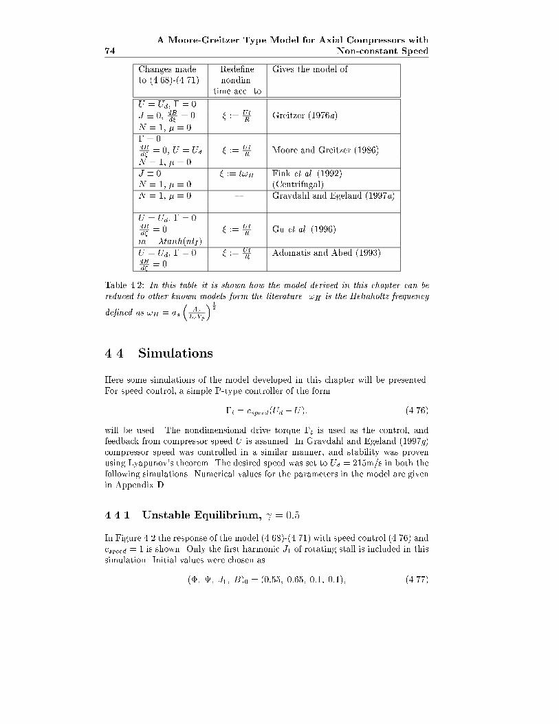
74
A Moore-Greitzer Type Model for Axial Compressors with
Non-constant Speed
Changes made Rede�ne Gives the model ofto (4.68)-(4.71) nondim.
time acc. to
U = Ud, � = 0
J � 0, dBd�
= 0 � := Ut
RGreitzer (1976a)
N = 1, � = 0
� = 0dB
d�= 0, U = Ud � := Ut
RMoore and Greitzer (1986)
N = 1, � = 0
J � 0 � := t!H Fink et al. (1992)N = 1, � = 0 (Centrifugal)
N = 1, � = 0 { Gravdahl and Egeland (1997a)
U = Ud, � = 0dB
d�= 0 � := Ut
RGu et al. (1996)
m = �tanh(nlI)
U = Ud, � = 0 � := Ut
RAdomatis and Abed (1993)
dB
d�= 0
Table 4.2: In this table it is shown how the model derived in this chapter can be
reduced to other known models form the literature. !H is the Helmholtz frequency
de�ned as !H = as
�Ac
LcVp
� 12
.
4.4 Simulations
Here some simulations of the model developed in this chapter will be presented.For speed control, a simple P-type controller of the form
�t = cspeed(Ud � U); (4.76)
will be used. The nondimensional drive torque �t is used as the control, andfeedback from compressor speed U is assumed. In Gravdahl and Egeland (1997g)compressor speed was controlled in a similar manner, and stability was provenusing Lyapunov's theorem. The desired speed was set to Ud = 215m/s in both thefollowing simulations. Numerical values for the parameters in the model are givenin Appendix D.
4.4.1 Unstable Equilibrium, = 0:5
In Figure 4.2 the response of the model (4.68)-(4.71) with speed control (4.76) andcspeed = 1 is shown. Only the �rst harmonic J1 of rotating stall is included in thissimulation. Initial values were chosen as
(�; ; J1; B)0 = (0:55; 0:65; 0:1; 0:1); (4.77)
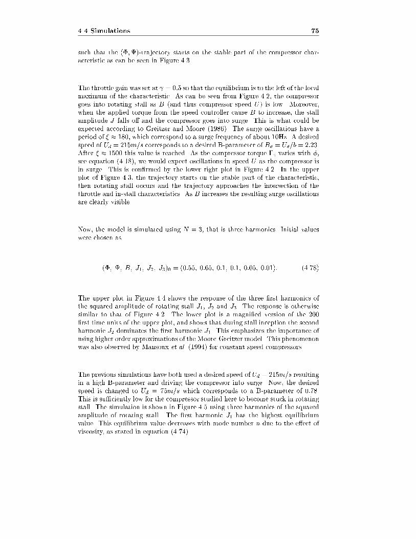
4.4 Simulations 75
such that the (�;)-trajectory starts on the stable part of the compressor char-acteristic as can be seen in Figure 4.3.
The throttle gain was set at = 0:5 so that the equilibrium is to the left of the localmaximum of the characteristic. As can be seen from Figure 4.2, the compressorgoes into rotating stall as B (and thus compressor speed U) is low. Moreover,when the applied torque from the speed controller cause B to increase, the stallamplitude J falls o� and the compressor goes into surge. This is what could beexpected according to Greitzer and Moore (1986). The surge oscillations have aperiod of � � 180, which correspond to a surge frequency of about 10Hz. A desiredspeed of Ud = 215m=s corresponds to a desired B-parameter of Bd = Ud=b = 2:23.After � � 1500 this value is reached. As the compressor torque �c varies with �,see equation (4.18), we would expect oscillations in speed U as the compressor isin surge. This is con�rmed by the lower right plot in Figure 4.2. In the upperplot of Figure 4.3, the trajectory starts on the stable part of the characteristic,then rotating stall occurs and the trajectory approaches the intersection of thethrottle and in-stall characteristics. As B increases the resulting surge oscillationsare clearly visible.
Now, the model is simulated using N = 3, that is three harmonics. Initial valueswere chosen as
(�; ; B; J1; J2; J3)0 = (0:55; 0:65; 0:1; 0:1; 0:05; 0:01): (4.78)
The upper plot in Figure 4.4 shows the response of the three �rst harmonics ofthe squared amplitude of rotating stall J1, J2 and J3. The response is otherwisesimilar to that of Figure 4.2. The lower plot is a magni�ed version of the 200�rst time units of the upper plot, and shows that during stall inception the secondharmonic J2 dominates the �rst harmonic J1. This emphasizes the importance ofusing higher order approximations of the Moore-Greitzer model. This phenomenonwas also observed by Mansoux et al. (1994) for constant speed compressors.
The previous simulations have both used a desired speed of Ud = 215m=s resultingin a high B-parameter and driving the compressor into surge. Now, the desiredspeed is changed to Ud = 75m=s which corresponds to a B-parameter of 0:78.This is su�ciently low for the compressor studied here to become stuck in rotatingstall. The simulation is shown in Figure 4.5 using three harmonics of the squaredamplitude of rotating stall. The �rst harmonic J1 has the highest equilibriumvalue. This equilibrium value decreases with mode number n due to the e�ect ofviscosity, as stated in equation (4.74).
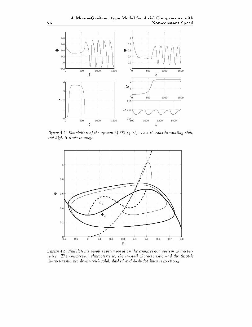
76
A Moore-Greitzer Type Model for Axial Compressors with
Non-constant Speed
0 500 1000 1500−0.2
0
0.2
0.4
0.6
0.8
0 500 1000 15000
0.2
0.4
0.6
0.8
1
0 500 1000 15000
1
2
3
4
0 500 1000 15000
1
2
800 1000 1200 1400214
215
216
��
��
�
J
B
U
Figure 4.2: Simulation of the system (4.68)-(4.71). Low B leads to rotating stall,
and high B leads to surge.
−0.2 −0.1 0 0.1 0.2 0.3 0.4 0.5 0.6 0.7 0.80
0.2
0.4
0.6
0.8
1
cc
ss
�
Figure 4.3: Simulations result superimposed on the compression system character-
istics. The compressor characteristic, the in-stall characteristic and the throttle
characteristic are drawn with solid, dashed and dash-dot lines respectively.
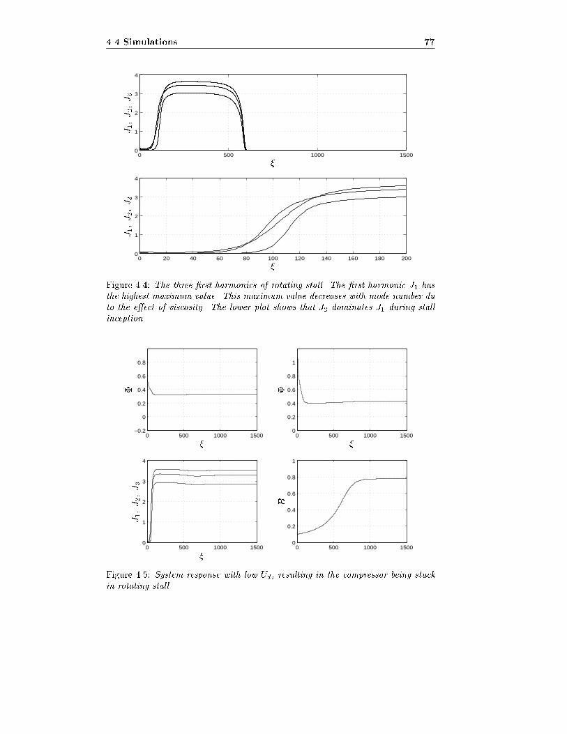
4.4 Simulations 77
0 500 1000 15000
1
2
3
4
0 20 40 60 80 100 120 140 160 180 2000
1
2
3
4
�
�
J1;J2;J3
J1;J2;J3
Figure 4.4: The three �rst harmonics of rotating stall. The �rst harmonic J1 has
the highest maximum value. This maximum value decreases with mode number du
to the e�ect of viscosity. The lower plot shows that J2 dominates J1 during stall
inception.
0 500 1000 1500−0.2
0
0.2
0.4
0.6
0.8
0 500 1000 15000
0.2
0.4
0.6
0.8
1
0 500 1000 15000
1
2
3
4
0 500 1000 15000
0.2
0.4
0.6
0.8
1
�
��
�
J1;J2;J3
B
Figure 4.5: System response with low Ud, resulting in the compressor being stuck
in rotating stall.
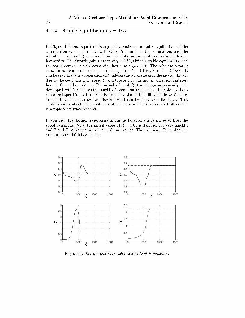
78
A Moore-Greitzer Type Model for Axial Compressors with
Non-constant Speed
4.4.2 Stable Equilibrium = 0:65
In Figure 4.6, the impact of the spool dynamics on a stable equilibrium of thecompression system is illustrated. Only J1 is used in this simulation, and theinitial values in (4.77) were used. Similar plots can be produced including higherharmonics. The throttle gain was set at = 0:65, giving a stable equilibrium, andthe speed controller gain was again chosen as cspeed = 1. The solid trajectoriesshow the system response to a speed change from U = 0:05m=s to U = 215m=s. Itcan be seen that the acceleration of U a�ects the other states of the model. This isdue to the couplings with speed U and torque � in the model. Of special interesthere, is the stall amplitude. The initial value of J(0) = 0:05 grows to nearly fullydeveloped rotating stall as the machine is accelerating, but is quickly damped outas desired speed is reached. Simulations show that this stalling can be avoided byaccelerating the compressor at a lower rate, that is by using a smaller cspeed. Thiscould possibly also be achieved with other, more advanced speed controllers, andis a topic for further research.
In contrast, the dashed trajectories in Figure 4.6 show the response without thespool dynamics. Now, the initial value J(0) = 0:05 is damped out very quickly,and � and converges to their equilibrium values. The transient e�ects observedare due to the initial conditions.
0 500 1000 15000.2
0.3
0.4
0.5
0.6
0.7
0.8
0 500 1000 15000.2
0.3
0.4
0.5
0.6
0.7
0.8
0 500 1000 15000
0.5
1
1.5
2
2.5
3
0 500 1000 15000
0.5
1
1.5
2
2.5
�
��
�
J B
Figure 4.6: Stable equilibrium with and without B-dynamics
4.5 Concluding Remarks 79
4.5 Concluding Remarks
In this chapter, a multi mode Moore-Greitzer axial compressor model with spooldynamics was derived. This resulted in a model with time varying B-parameter.Through simulations it was demonstrated that the model was capable of demon-strating both rotating stall and surge, and that the type of instability dependedon the compressor speed. Compressor speed was controlled with a simple pro-portional control law. In the original Moore Greitzer model only the �rst modeof rotating stall is included. The simulations in this chapter show that duringstall inception, higher order modes can dominate the �rst mode. This is in accor-dance with known results, and is shown here to be valid also for variable speedcompressors.
Further work on this topic includes 1) Stability analysis and stall/surge controldesign for variable speed axial compressors and 2) The use of simultaneous speedcontrol and stall/surge control to achieve rapid acceleration without stalling thecompressor.

80
A Moore-Greitzer Type Model for Axial Compressors with
Non-constant Speed
Chapter 5
Modelling and Control of
Surge for a Centrifugal
Compressor with
Non-constant Speed
5.1 Introduction
In this chapter the compressor characteristic for a variable speed centrifugal com-pressor is investigated. This characteristic is incooperated in a model similar tothat of Fink et al. (1992), and surge phenomena is studied in connection withvarying compressor speed. Energy losses in the compressor components is used toderive the characteristic, making a departure from the usual cubic characteristicmost commonly encountered in the surge control literature. Inspired by Ferguson(1963) and Watson and Janota (1982), uid friction and incidence losses, as well asother losses, in the compressor components are modeled, and a variable speed com-pressor characteristic is developed based on this. Both annular and vaned di�usersare studied. Surge and speed controllers for variable speed centrifugal compressorsare presented and analyzed. The speed is controlled with a PI-control law.
Axial and centrifugal compressors mostly show similar ow instabilities, but incentrifugal compressors, the matching between components, such as impeller anddi�user, in uences the stability properties. According to Emmons et al. (1955),de Jager (1995) and others, rotating stall is believed to have little e�ect on cen-trifugal compressor performance. The modeling and analysis in this chapter isthus restricted to surge. Hansen et al. (1981) showed that the model of Greitzer(1976a) is also applicable to centrifugal compressors, and this model will also beused here.
Since compressors are variable speed machines, it is of interest to investigate the
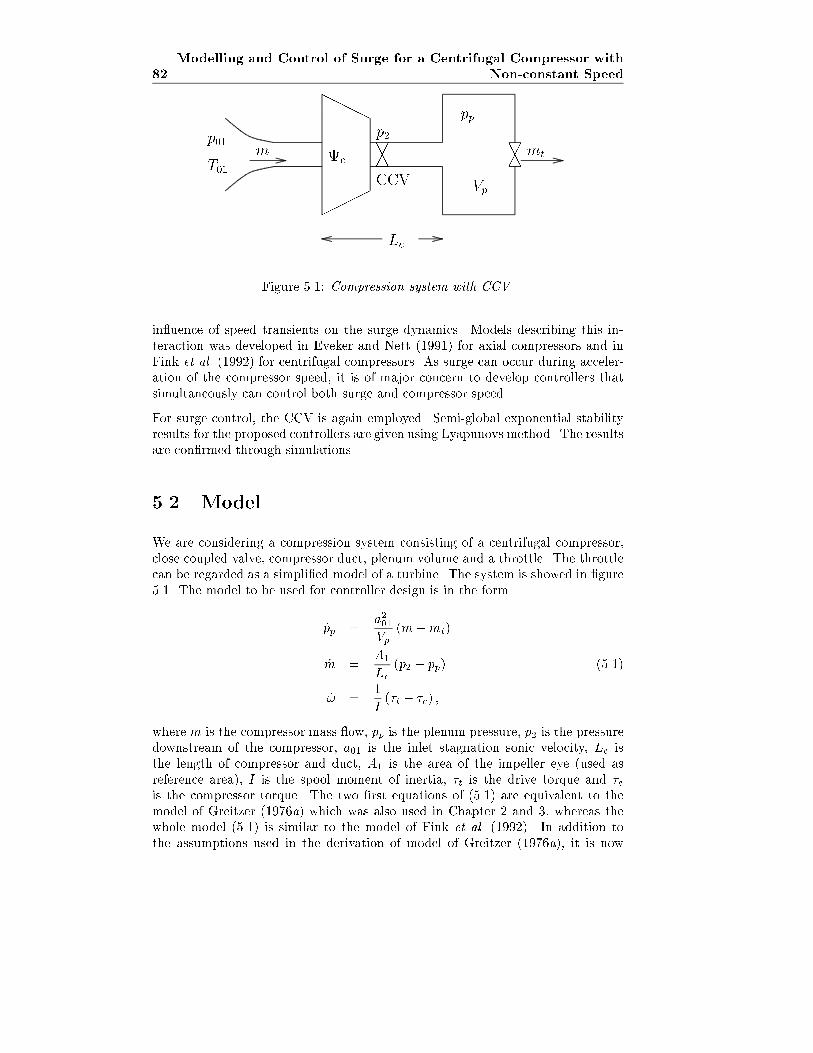
82
Modelling and Control of Surge for a Centrifugal Compressor with
Non-constant Speed
HHHH
����
AA��A
A��
p2
CCV
pp
Vp
Lc
c
p01
T01
m mt
Figure 5.1: Compression system with CCV.
in uence of speed transients on the surge dynamics. Models describing this in-teraction was developed in Eveker and Nett (1991) for axial compressors and inFink et al. (1992) for centrifugal compressors. As surge can occur during acceler-ation of the compressor speed, it is of major concern to develop controllers thatsimultaneously can control both surge and compressor speed.
For surge control, the CCV is again employed. Semi-global exponential stabilityresults for the proposed controllers are given using Lyapunovs method. The resultsare con�rmed through simulations.
5.2 Model
We are considering a compression system consisting of a centrifugal compressor,close coupled valve, compressor duct, plenum volume and a throttle. The throttlecan be regarded as a simpli�ed model of a turbine. The system is showed in �gure5.1. The model to be used for controller design is in the form
_pp =a201Vp
(m�mt)
_m =A1
Lc(p2 � pp) (5.1)
_! =1
I(�t � �c) ;
where m is the compressor mass ow, pp is the plenum pressure, p2 is the pressuredownstream of the compressor, a01 is the inlet stagnation sonic velocity, Lc isthe length of compressor and duct, A1 is the area of the impeller eye (used asreference area), I is the spool moment of inertia, �t is the drive torque and �cis the compressor torque. The two �rst equations of (5.1) are equivalent to themodel of Greitzer (1976a) which was also used in Chapter 2 and 3, whereas thewhole model (5.1) is similar to the model of Fink et al. (1992). In addition tothe assumptions used in the derivation of model of Greitzer (1976a), it is now
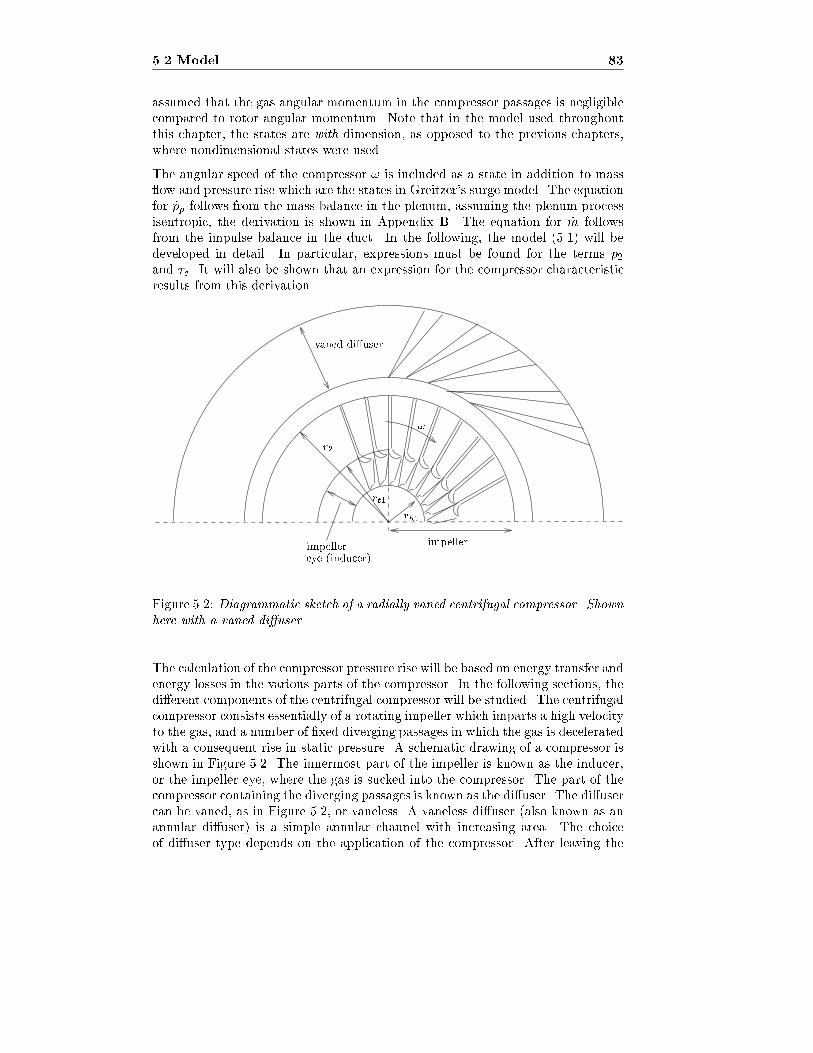
5.2 Model 83
assumed that the gas angular momentum in the compressor passages is negligiblecompared to rotor angular momentum. Note that in the model used throughoutthis chapter, the states are with dimension, as opposed to the previous chapters,where nondimensional states were used.
The angular speed of the compressor ! is included as a state in addition to mass ow and pressure rise which are the states in Greitzer's surge model. The equationfor _pp follows from the mass balance in the plenum, assuming the plenum processisentropic, the derivation is shown in Appendix B. The equation for _m followsfrom the impulse balance in the duct. In the following, the model (5.1) will bedeveloped in detail. In particular, expressions must be found for the terms p2and �c. It will also be shown that an expression for the compressor characteristicresults from this derivation.
vaned di�user
eye (inducer)
rh1
r2
impellerimpeller
!
rt1
Figure 5.2: Diagrammatic sketch of a radially vaned centrifugal compressor. Shownhere with a vaned di�user.
The calculation of the compressor pressure rise will be based on energy transfer andenergy losses in the various parts of the compressor. In the following sections, thedi�erent components of the centrifugal compressor will be studied. The centrifugalcompressor consists essentially of a rotating impeller which imparts a high velocityto the gas, and a number of �xed diverging passages in which the gas is deceleratedwith a consequent rise in static pressure. A schematic drawing of a compressor isshown in Figure 5.2. The innermost part of the impeller is known as the inducer,or the impeller eye, where the gas is sucked into the compressor. The part of thecompressor containing the diverging passages is known as the di�user. The di�usercan be vaned, as in Figure 5.2, or vaneless. A vaneless di�user (also known as anannular di�user) is a simple annular channel with increasing area. The choiceof di�user type depends on the application of the compressor. After leaving the
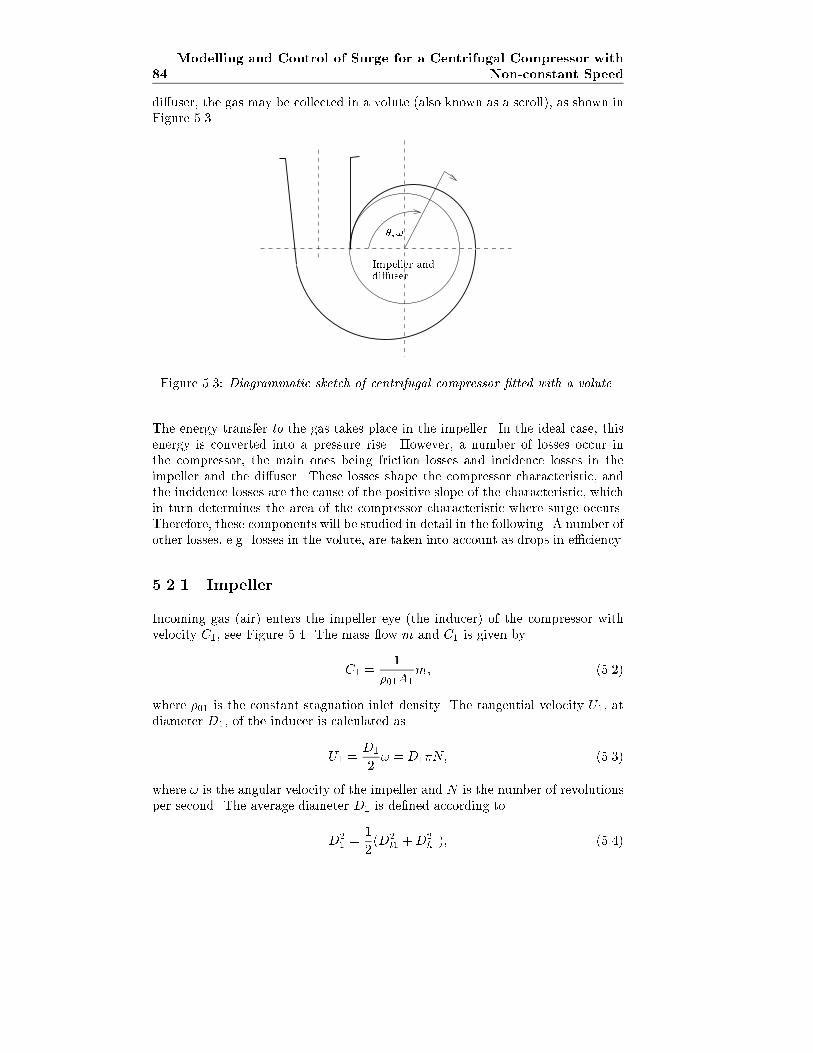
84
Modelling and Control of Surge for a Centrifugal Compressor with
Non-constant Speed
di�user, the gas may be collected in a volute (also known as a scroll), as shown inFigure 5.3.
�; !
Impeller anddi�user
Figure 5.3: Diagrammatic sketch of centrifugal compressor �tted with a volute.
The energy transfer to the gas takes place in the impeller. In the ideal case, thisenergy is converted into a pressure rise. However, a number of losses occur inthe compressor, the main ones being friction losses and incidence losses in theimpeller and the di�user. These losses shape the compressor characteristic, andthe incidence losses are the cause of the positive slope of the characteristic, whichin turn determines the area of the compressor characteristic where surge occurs.Therefore, these components will be studied in detail in the following. A number ofother losses, e.g. losses in the volute, are taken into account as drops in e�ciency.
5.2.1 Impeller
Incoming gas (air) enters the impeller eye (the inducer) of the compressor withvelocity C1, see Figure 5.4. The mass ow m and C1 is given by
C1 =1
�01A1m; (5.2)
where �01 is the constant stagnation inlet density. The tangential velocity U1, atdiameter D1, of the inducer is calculated as
U1 =D1
2! = D1�N; (5.3)
where ! is the angular velocity of the impeller and N is the number of revolutionsper second. The average diameter D1 is de�ned according to
D21 =
1
2(D2
t1 +D2h1); (5.4)
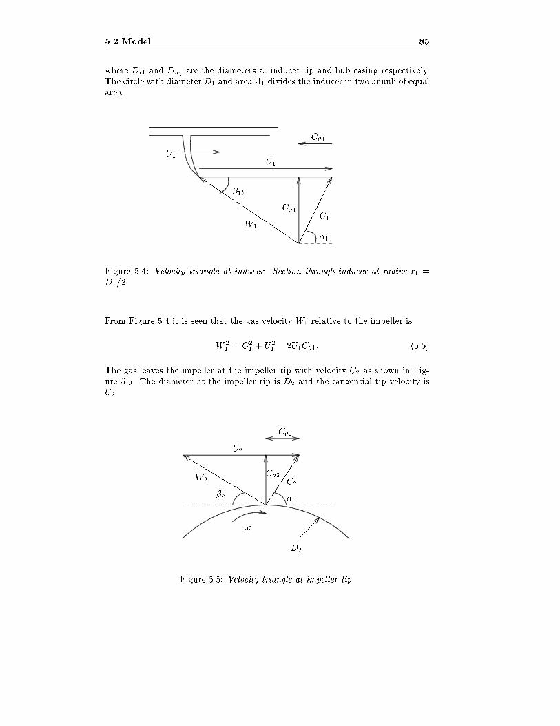
5.2 Model 85
where Dt1 and Dh1are the diameters at inducer tip and hub casing respectively.
The circle with diameter D1 and area A1 divides the inducer in two annuli of equalarea.
Q
��������
U1
C�1
C1Ca1
W1
�1
�1b
U1
Figure 5.4: Velocity triangle at inducer. Section through inducer at radius r1 =D1=2.
From Figure 5.4 it is seen that the gas velocity W1 relative to the impeller is
W 21 = C2
1 + U21 � 2U1C�1: (5.5)
The gas leaves the impeller at the impeller tip with velocity C2 as shown in Fig-ure 5.5. The diameter at the impeller tip is D2 and the tangential tip velocity isU2.
bb
bb
bbb
bbb
���
U2
�2
W2Ca2
C2
�2
!
D2
C�2
Figure 5.5: Velocity triangle at impeller tip.
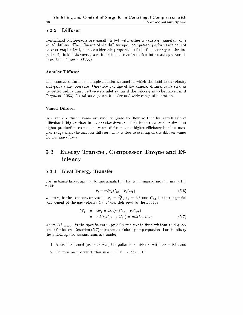
86
Modelling and Control of Surge for a Centrifugal Compressor with
Non-constant Speed
5.2.2 Di�user
Centrifugal compressors are usually �tted with either a vaneless (annular) or avaned di�user. The in uence of the di�user upon compressor performance cannotbe over emphasized, as a considerable proportion of the uid energy at the im-peller tip is kinetic energy and its e�cient transformation into static pressure isimportant Ferguson (1963).
Annular Di�user
The annular di�user is a simple annular channel in which the uid loses velocityand gains static pressure. One disadvantage of the annular di�user is its size, asits outlet radius must be twice its inlet radius if the velocity is to be halved in itFerguson (1963). Its advantages are its price and wide range of operation.
Vaned Di�user
In a vaned di�user, vanes are used to guide the ow so that he overall rate ofdi�usion is higher than in an annular di�user. This leads to a smaller size, buthigher production costs. The vaned di�user has a higher e�ciency but less mass ow range than the annular di�user. This is due to stalling of the di�user vanesfor low mass ows.
5.3 Energy Transfer, Compressor Torque and Ef-
�ciency
5.3.1 Ideal Energy Transfer
For turbomachines, applied torque equals the change in angular momentum of the uid:
�c = m(r2C�2 � r1C�1); (5.6)
where �c is the compressor torque, r1 = D1
2, r2 = D2
2and C�2 is the tangential
component of the gas velocity C2. Power delivered to the uid is
_Wc = !�c = !m(r2C�2 � r1C�1)
= m(U2C�2 �1 C�1) = m�h0c;ideal (5.7)
where �h0c;ideal is the speci�c enthalpy delivered to the uid without taking ac-count for losses. Equation (5.7) is known as Euler's pump equation. For simplicitythe following two assumptions are made:
1. A radially vaned (no backsweep) impeller is considered with �2b = 90�, and
2. There is no pre-whirl, that is �1 = 90� ) C�1 = 0.
5.3 Energy Transfer, Compressor Torque and E�ciency 87
The slip factor is de�ned as
�4=C�2
U2� 1� 2
i: (5.8)
The approximation is known as Stanitz' formula where i is the number of compres-sor blades. From (5.7), and using (5.8), we have that the ideal speci�c enthalpydelivered to the uid is
�h0c;ideal =_Wc;ideal
m= �U2
2 : (5.9)
Notice that �h0c;ideal is independent of mass owm, and ideally we would have thesame energy transfer for all mass ows1. However, due to various losses, the energytransfer is not constant, and we now include this in the analysis. According toWatson and Janota (1982), Ferguson (1963), Nisenfeld (1982) and other authors,the two major losses, expressed as speci�c enthalpies, are:
1. Incidence losses in impeller and di�user, �hii and �hid
2. Fluid friction losses in impeller and di�user, �hfi and �hfd
The incidence losses and uid friction losses play an important role in determiningthe region of stable operation for the compressor. Other losses, such as back owlosses, clearance losses and losses in the volute will be taken into account whencomputing the e�ciency of the compressor. There also exist other losses such asinlet casing losses, mixing losses and leakage losses, but these will be ignored in thefollowing. For a further treatment on this topic, some references are Balj�e (1952),Johnston and Dean, Jr. (1966), Whit�eld and Wallace (1975) and Cumpsty (1989).
5.3.2 Compressor Torque
Using the assumption of no pre whirl and equation (5.6), the compressor torque is
�+c= mr2C�2 = mr2�U2; m > 0: (5.10)
The torque calculated in (5.10) is for forward ow. However, the compressor mayenter deep surge, that is reversal of ow, and there is need for an expression for thecompressor torque at negative mass ow. According to Ko� and Greitzer (1986),an axial compressor in reversed ow can be viewed as a throttling device. Hereit is assumed that a centrifugal compressor in reversed ow can be approximatedwith a turbine. This allows for the use of Euler's turbine equation:
��c= m(r1C�1 � r2C�2) = �mr2�U2; m < 0: (5.11)
Combination of (5.10) and (5.11) gives
�c = jmjr2�U2; 8m (5.12)
which is in accordance with the compressor torque used by Fink et al. (1992).
1If backswept impeller blades, �2b < 90�, were considered, �h0c;ideal would decrease with
increasing m.
88
Modelling and Control of Surge for a Centrifugal Compressor with
Non-constant Speed
Disc Friction Torque
The torque set up by the rotation of the impeller in a uid is modeled as rotationof a disc. When a disc is rotated in a uid, a resistive torque is set up given by
�df = 2
Zr2
r1
�tan2�r2dr; (5.13)
where r1 is the radius of the shaft, r2 is the radius of the disc and �tan is thetangential component of the shear stress between the disc and uid. According toFerguson (1963) the torque can be approximated by
�df =Cm�r
52!
2
2=
2Cm�r52
D21
U21 (5.14)
where Cm is a torque coe�cient depending on the disc Reynolds number and thespace between the disc and the casing, � is the density of the uid and ! is theangular velocity of the disc. In (5.14) it has been assumed that r1 << r2.
5.3.3 Incidence Losses
The losses due to incidence onto the rotor and vaned di�user play an importantrole in shaping the compressor characteristic. There exists several methods ofmodeling this loss, and a comparative study is given by Whit�eld and Wallace(1973). The two most widely used approaches are:
(1) The so called \NASA shock loss theory" reported in Watson and Janota(1982) and Whit�eld and Wallace (1973), which is based upon the tangentialcomponent of kinetic energy being destroyed.
(2) A constant pressure incidence model reported by Whit�eld and Wallace(1973) where it is assumed that the ow just inside the blades has adaptedto the blades via a constant pressure process.
Watson and Janota (1982) concludes that for centrifugal compressors, the di�er-ences between the two models are small. According to Whit�eld and Wallace(1973), the main di�erence lies in the prediction of the incidence angle at whichzero loss occurs. For model (1) zero loss is predicted when the ow angle at theinlet equals the blade angle. This is not the case for model (2). Based on this,and the simplicity of (1), the NASA shock loss theory is used here. As Ferguson(1963) points out, the term shock loss is misleading as nothing akin to shock oc-curs in practice, but the simple notion of shock is used to explain the shape of thecompressor characteristic.
Depending on whether the mass ow is lower or higher than the design ow,positive or negative stall is said to occur. The use of model (2) leads to a lossvarying with the square of the mass ow, symmetrical about the design ow.Ferguson (1963) states that the incidence loss in practice increase more rapidly
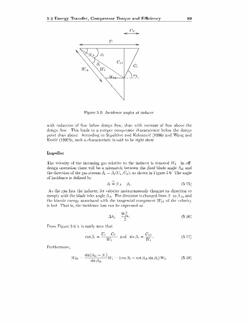
5.3 Energy Transfer, Compressor Torque and E�ciency 89
eeeeeeeeeeeeee
eeeeeeee
��������Q
U1
C�1
C1Ca1
W1
�1
W1b
W�1
�i
�1�1b
Figure 5.6: Incidence angles at inducer.
with reduction of ow below design ow, than with increase of ow above thedesign ow. This leads to a steeper compressor characteristic below the designpoint than above. According to Sepulchre and Kokotovi�c (1996) and Wang andKrsti�c (1997b), such a characteristic is said to be right skew.
Impeller
The velocity of the incoming gas relative to the inducer is denoted W1. In o�-design operation there will be a mismatch between the �xed blade angle �1b andthe direction of the gas stream �1 = �1(U1; C1), as shown in Figure 5.6. The angleof incidence is de�ned by
�i4= �1b � �1: (5.15)
As the gas hits the inducer, its velocity instantaneously changes its direction tocomply with the blade inlet angle �1b. The direction is changed from �1 to �1b, andthe kinetic energy associated with the tangential component W�1 of the velocityis lost. That is, the incidence loss can be expressed as
�hi =W 2�1
2: (5.16)
From Figure 5.6 it is easily seen that
cos�1 =U1 � C�1
W1
and sin�1 =Ca1
W1
: (5.17)
Furthermore,
W�1 =sin(�1b � �1)
sin�1bW1 = (cos�1 � cot�1b sin�1)W1: (5.18)
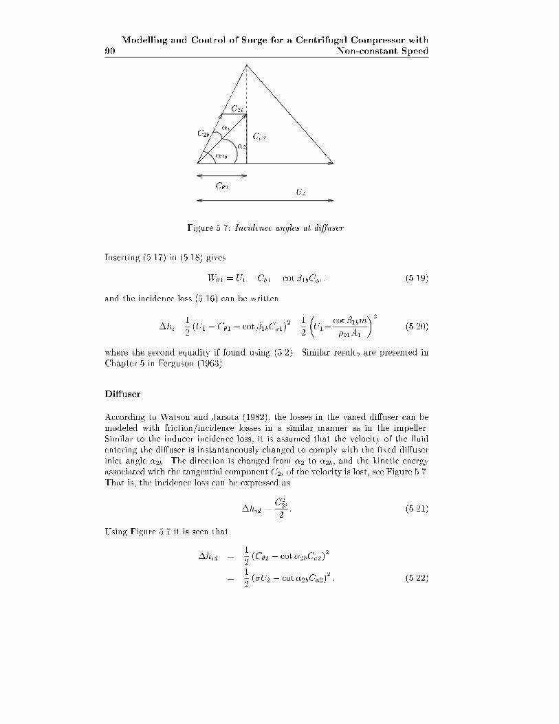
90
Modelling and Control of Surge for a Centrifugal Compressor with
Non-constant Speed
������
eeeeeeeeeeee�
�����������
C�2U2
�2b
�i
�2
Ca2C2b
C2i
Figure 5.7: Incidence angles at di�user.
Inserting (5.17) in (5.18) gives
W�1 = U1 � C�1 � cot�1bCa1: (5.19)
and the incidence loss (5.16) can be written
�hi=1
2(U1 � C�1 � cot�1bCa1)
2=1
2
�U1� cot�1bm
�01A1
�2(5.20)
where the second equality if found using (5.2). Similar results are presented inChapter 5 in Ferguson (1963).
Di�user
According to Watson and Janota (1982), the losses in the vaned di�user can bemodeled with friction/incidence losses in a similar manner as in the impeller.Similar to the inducer incidence loss, it is assumed that the velocity of the uidentering the di�user is instantaneously changed to comply with the �xed di�userinlet angle �2b. The direction is changed from �2 to �2b, and the kinetic energyassociated with the tangential component C2i of the velocity is lost, see Figure 5.7.That is, the incidence loss can be expressed as
�hid =C22i
2: (5.21)
Using Figure 5.7 it is seen that
�hid =1
2(C�2 � cot�2bCa2)
2
=1
2(�U2 � cot�2bCa2)
2: (5.22)
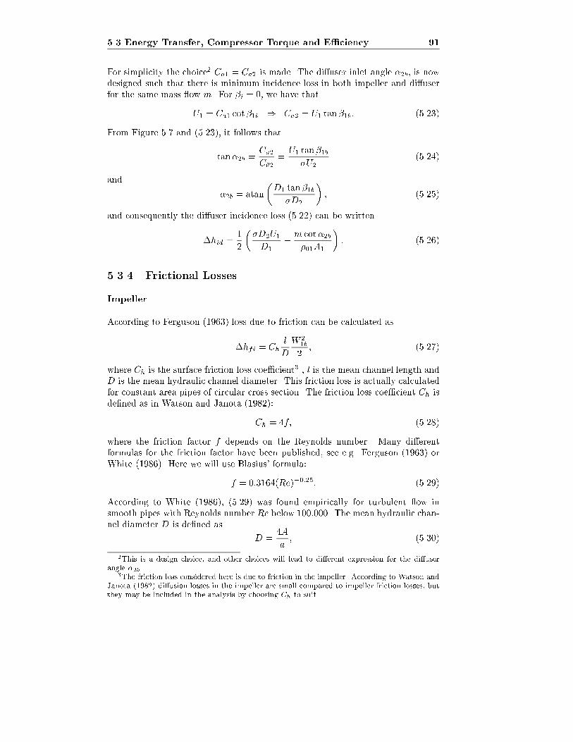
5.3 Energy Transfer, Compressor Torque and E�ciency 91
For simplicity the choice2 Ca1 = Ca2 is made. The di�user inlet angle �2b, is nowdesigned such that there is minimum incidence loss in both impeller and di�userfor the same mass ow m. For �i = 0, we have that
U1 = Ca1 cot�1b ) Ca2 = U1 tan�1b: (5.23)
From Figure 5.7 and (5.23), it follows that
tan�2b =Ca2
C�2=U1 tan�1b
�U2(5.24)
and
�2b = atan
�D1 tan�1b�D2
�; (5.25)
and consequently the di�user incidence loss (5.22) can be written
�hid =1
2
��D2U1
D1
� m cot�2b�01A1
�: (5.26)
5.3.4 Frictional Losses
Impeller
According to Ferguson (1963) loss due to friction can be calculated as
�hfi = Chl
D
W 21b
2; (5.27)
where Ch is the surface friction loss coe�cient3 , l is the mean channel length andD is the mean hydraulic channel diameter. This friction loss is actually calculatedfor constant area pipes of circular cross section. The friction loss coe�cient Ch isde�ned as in Watson and Janota (1982):
Ch = 4f; (5.28)
where the friction factor f depends on the Reynolds number. Many di�erentformulas for the friction factor have been published, see e.g. Ferguson (1963) orWhite (1986). Here we will use Blasius' formula:
f = 0:3164(Re)�0:25: (5.29)
According to White (1986), (5.29) was found empirically for turbulent ow insmooth pipes with Reynolds number Re below 100:000. The mean hydraulic chan-nel diameter D is de�ned as
D =4A
a; (5.30)
2This is a design choice, and other choices will lead to di�erent expression for the di�user
angle �2b3The friction loss considered here is due to friction in the impeller. According to Watson and
Janota (1982) di�usion losses in the impeller are small compared to impeller friction losses, but
they may be included in the analysis by choosing Ch to suit.
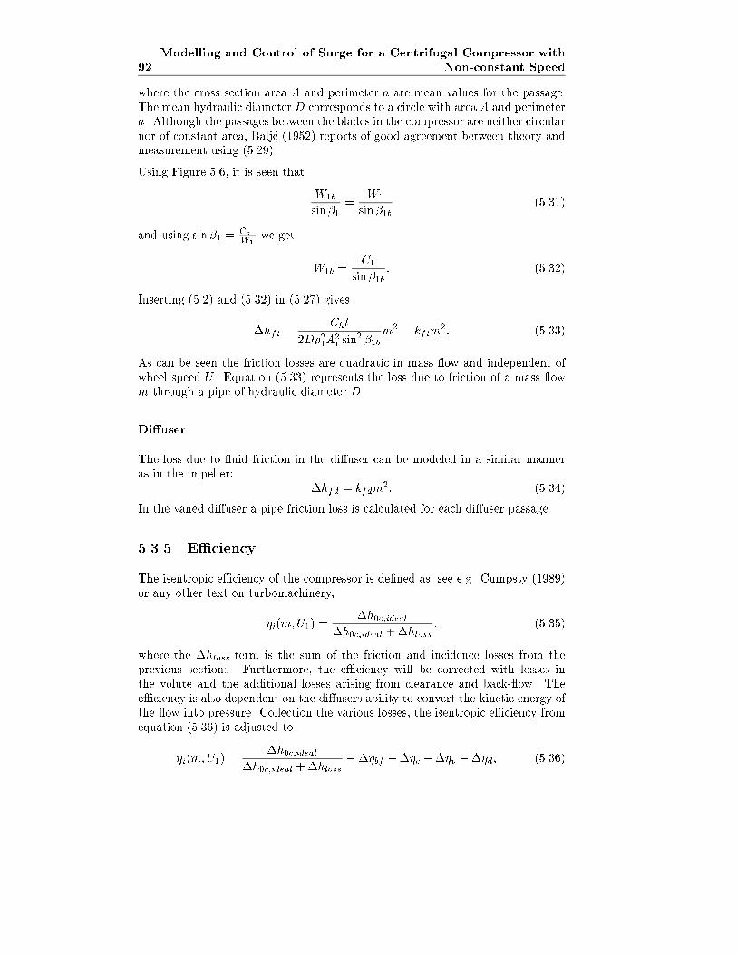
92
Modelling and Control of Surge for a Centrifugal Compressor with
Non-constant Speed
where the cross section area A and perimeter a are mean values for the passage.The mean hydraulic diameter D corresponds to a circle with area A and perimetera. Although the passages between the blades in the compressor are neither circularnor of constant area, Balj�e (1952) reports of good agreement between theory andmeasurement using (5.29).
Using Figure 5.6, it is seen that
W1b
sin�1=
W1
sin�1b(5.31)
and using sin�1 =Ca1
W1we get
W1b =C1
sin�1b: (5.32)
Inserting (5.2) and (5.32) in (5.27) gives
�hfi =Chl
2D�21A21 sin
2 �1bm2 = kfim
2: (5.33)
As can be seen the friction losses are quadratic in mass ow and independent ofwheel speed U . Equation (5.33) represents the loss due to friction of a mass owm through a pipe of hydraulic diameter D.
Di�user
The loss due to uid friction in the di�user can be modeled in a similar manneras in the impeller:
�hfd = kfdm2: (5.34)
In the vaned di�user a pipe friction loss is calculated for each di�user passage.
5.3.5 E�ciency
The isentropic e�ciency of the compressor is de�ned as, see e.g. Cumpsty (1989)or any other text on turbomachinery,
�i(m;U1) =�h0c;ideal
�h0c;ideal +�hloss: (5.35)
where the �hloss-term is the sum of the friction and incidence losses from theprevious sections. Furthermore, the e�ciency will be corrected with losses inthe volute and the additional losses arising from clearance and back- ow. Thee�ciency is also dependent on the di�users ability to convert the kinetic energy ofthe ow into pressure. Collection the various losses, the isentropic e�ciency fromequation (5.36) is adjusted to
�i(m;U1) =�h0c;ideal
�h0c;ideal +�hloss���bf ���c ���v ���d; (5.36)
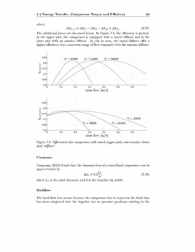
5.3 Energy Transfer, Compressor Torque and E�ciency 93
where�hloss = �hif +�hii +�hdf +�hdi: (5.37)
The additional losses are discussed below. In Figure 5.8, the e�ciency is plotted.In the upper plot, the compressor is equipped with a vaned di�user and in thelower plot with an annular di�user. As can be seen, the vaned di�user o�er ahigher e�ciency, but a narrower range of ow compared with the annular di�user.
0 0.1 0.2 0.3 0.4 0.5 0.60.6
0.65
0.7
0.75
0.8
0.85
0 0.1 0.2 0.3 0.4 0.5 0.60.6
0.65
0.7
0.75
0.8
0.85
�i;vaned
�i;annular
mass ow [kg/s]
mass ow [kg/s]
N = 20000
N = 20000
N = 35000
N = 35000
N = 50000
N = 50000
Figure 5.8: E�ciencies for compressor with vaned (upper plot) and annular (lower
plot) di�user.
Clearance
Pampreen (1973) found that the clearance loss of a centrifugal compressor can beapproximated by
��c = 0:3lcl
b; (5.38)
where lcl is the axial clearance and b is the impeller tip width.
Back ow
The back- ow loss occurs because the compressor has to reprocess the uid thathas been reinjected into the impeller due to pressure gradients existing in the
94
Modelling and Control of Surge for a Centrifugal Compressor with
Non-constant Speed
impeller tip region. Due to the lack of accurate modeling of this loss, Watson andJanota (1982) suggest a loss of 3 points of e�ciency as typical:
��bf = 0:03: (5.39)
Volute
In the volute a loss will take place mainly due to the inability of the volute to usethe radial kinetic energy out of the di�user. Cumpsty (1989) assumes this loss tolie within 2-5 point of e�ciency:
0:02 � ��v � 0:05: (5.40)
This loss is likely to be higher for compressor with a vaned di�user than with anannular di�user, as a larger part of the total kinetic energy at the outlet of thevaned di�user is in the radial direction. A more comprehensive treatment of lossin volutes can be found in Lorett and Gopalakrishnan (1986).
Di�usion
The purpose of the di�user is decelerate the ow with high kinetic energy, and thusconvert this into pressure. This can be achieved more or less e�cient dependingon the construction of the di�user. Due to inadequate di�usion in the di�userthere will be a degradation ��d in the e�ciency �i. The e�ciency drop ��dis dependent on the pressure recovery coe�cient, see e.g. Cumpsty (1989) orWatson and Janota (1982), but for simplicity ��d will be considered constanthere. According to Watson and Janota (1982) vaned di�users o�er a 2 to 7 pointsincrease in e�ciency compared to annular di�users.
5.4 Energy Transfer and Pressure Rise
Including the losses, the total speci�c energy transfer can be calculated by sub-tracting (5.33), (5.20), (5.26) and (5.34) from (5.9):
�h0c(U1;m) = �h0c;ideal ��hif ��hii ��hdf ��hdi: (5.41)
�h0c is a second degree polynomial in m, and as opposed to the ideal case, we seethat energy transfer to the uid is varying with mass ow m. This is shown inFigure 5.9.
To �nd an expression for the pressure rise we now need a relation between pressurerise and energy transfer. The pressure rise is modeled as
p2 =
�1 +
�i(m;U1)�h0c;idealT01cp
� �
��1
p01 = c(U1;m)p01; (5.42)
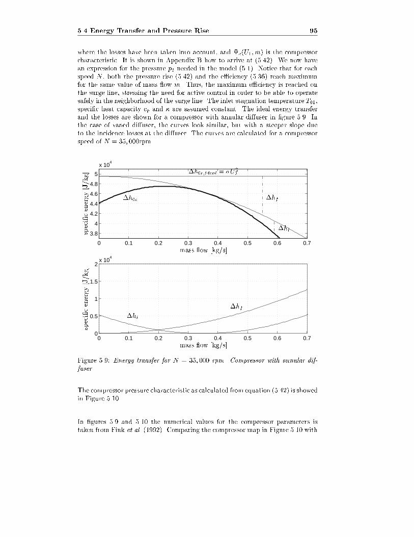
5.4 Energy Transfer and Pressure Rise 95
where the losses have been taken into account, and c(U1;m) is the compressorcharacteristic. It is shown in Appendix B how to arrive at (5.42). We now havean expression for the pressure p2 needed in the model (5.1). Notice that for eachspeed N , both the pressure rise (5.42) and the e�ciency (5.36) reach maximumfor the same value of mass ow m. Thus, the maximum e�ciency is reached onthe surge line, stressing the need for active control in order to be able to operatesafely in the neighborhood of the surge line. The inlet stagnation temperature T01,speci�c heat capacity cp and � are assumed constant. The ideal energy transferand the losses are shown for a compressor with annular di�user in �gure 5.9. Inthe case of vaned di�user, the curves look similar, but with a steeper slope dueto the incidence losses at the di�user. The curves are calculated for a compressorspeed of N = 35; 000rpm.
0 0.1 0.2 0.3 0.4 0.5 0.6 0.7
3.8
4
4.2
4.4
4.6
4.8
5
x 104
0 0.1 0.2 0.3 0.4 0.5 0.6 0.70
0.5
1
1.5
2x 10
4
�h0c;ideal = �U22
�h0c
�hi
�hi
�hf
�hf
mass ow [kg/s]
mass ow [kg/s]
speci�cenergy[J/kg]
speci�cenergy[J/kg]
Figure 5.9: Energy transfer for N = 35; 000 rpm. Compressor with annular dif-
fuser.
The compressor pressure characteristic as calculated from equation (5.42) is showedin Figure 5.10.
In �gures 5.9 and 5.10 the numerical values for the compressor parameters istaken from Fink et al. (1992). Comparing the compressor map in Figure 5.10 with
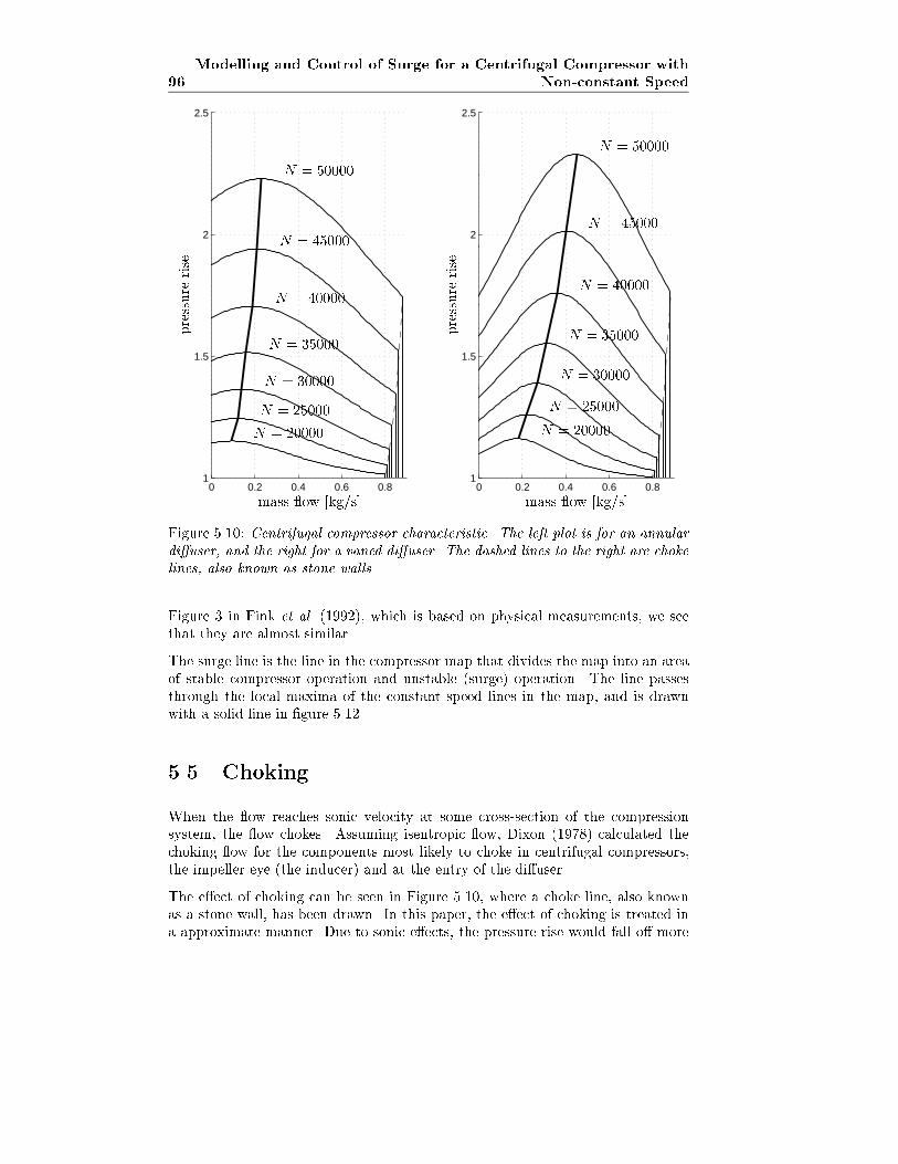
96
Modelling and Control of Surge for a Centrifugal Compressor with
Non-constant Speed
0 0.2 0.4 0.6 0.81
1.5
2
2.5
0 0.2 0.4 0.6 0.81
1.5
2
2.5
N = 20000N = 20000
N = 25000N = 25000
N = 30000N = 30000
N = 35000N = 35000
N = 40000N = 40000
N = 45000
N = 45000
N = 50000
N = 50000
mass ow [kg/s]mass ow [kg/s]
pressurerise
pressurerise
Figure 5.10: Centrifugal compressor characteristic. The left plot is for an annular
di�user, and the right for a vaned di�user. The dashed lines to the right are choke
lines, also known as stone walls.
Figure 3 in Fink et al. (1992), which is based on physical measurements, we seethat they are almost similar.
The surge line is the line in the compressor map that divides the map into an areaof stable compressor operation and unstable (surge) operation. The line passesthrough the local maxima of the constant speed lines in the map, and is drawnwith a solid line in �gure 5.12.
5.5 Choking
When the ow reaches sonic velocity at some cross-section of the compressionsystem, the ow chokes. Assuming isentropic ow, Dixon (1978) calculated thechoking ow for the components most likely to choke in centrifugal compressors,the impeller eye (the inducer) and at the entry of the di�user.
The e�ect of choking can be seen in Figure 5.10, where a choke line, also knownas a stone wall, has been drawn. In this paper, the e�ect of choking is treated ina approximate manner. Due to sonic e�ects, the pressure rise would fall o� more
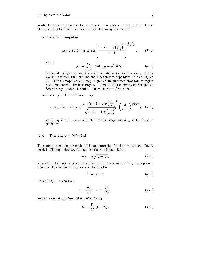
5.6 Dynamic Model 97
gradually when approaching the stone wall than shown in Figure 5.10. Dixon(1978) showed that the mass ows for which choking occurs are:
� Choking in impeller
mchoke(U1) = A1�01a01
2642 + (�� 1)
�U1
a01
�2�+ 1
375
(�+1)
2(��1)
; (5.43)
where�01 =
p01
RT01and a01 =
p�RT01 (5.44)
is the inlet stagnation density and inlet stagnation sonic velocity, respec-tively. It is seen than the choking mass ow is dependent on blade speedU1. Thus the impeller can accept a greater limiting mass ow rate at higherrotational speeds. By inserting U1 = 0 in (5.43) the expression for choked ow through a nozzle is found. This is shown in Appendix B.
� Choking in the di�user entry
mchoke(U2) = A4�01a01
1 + (�� 1)�imp��U2
a01
�2r1 + (�� 1)�
�U2
a01
�2�
2
�+ 1
� (�+1)
2(��1)
; (5.45)
where A4 is the ow area of the di�user entry, and �imp is the impellere�ciency.
5.6 Dynamic Model
To complete the dynamic model (5.1), an expression for the throttle mass ow isneeded. The mass ow mt through the throttle is modeled as
mt = ktppp � p01; (5.46)
where kt is the throttle gain proportional to throttle opening and pp is the plenumpressure. The momentum balance of the spool is
I _! = �t � �c: (5.47)
Using (5.3) it is seen that
! =2U1D1
) _! =2 _U1D1
; (5.48)
and thus we get a di�erential equation for U1,
_U1 =D1
2I(�t � �c) : (5.49)
98
Modelling and Control of Surge for a Centrifugal Compressor with
Non-constant Speed
The drive torque �t may be delivered by a turbine, and will be used as a controlvariable for speed control. The compressor and spool can only rotate in onedirection, and the speed is assumed upper bounded:
0 � U1(t) < Um: (5.50)
Using (5.12) and (5.49), and inserting equations (5.42) and (5.46) in (5.1), we getthe following dynamic model for the compression system
_pp =a201Vp
(m� ktppp � p01)
_m =A
L
�1 +
�i(m;U1)�h0c;idealT01cp
� �
��1
p01 � pp
!(5.51)
_U1 =D1
2I(�t � �c) :
It is worth noticing that a time varying U is equivalent with a time varying B-parameter Fink et al. (1992). Greitzer's B-parameter as de�ned in Greitzer (1976a)
is given by B = U1
2a01
qVp
A1Lc; where Vp is the plenum volume and Lc is the length
of the compressor and duct. Using (5.49), a nonlinear di�erential equation for Bcan be found.
5.7 Surge Control Idea
The reason for equilibria to the left of the surge line being unstable, and causingthe compressor to go into surge, is the positive slope of the characteristic in thisarea. From Figure 5.9 it is seen that the positive slope is due to the incidence lossesat low mass ows. From the expression for the incidence loss, equation (5.20), itis clear that a variable blade angle �1b would make it possible to minimize theincidence losses over a range of mass ows. Thus variable inducer blades might beused as a means of surge stabilization.
On the other hand, the maximum energy transfer and minimum incidence loss donot occur for the same mass ow. This is due to the friction losses. The frictionshifts the point of maximum energy transfer, and consequently pressure rise, tothe left of the point of minimum incidence loss. From this, we conclude that thefriction losses in fact have a stabilizing e�ect, and introducing additional uidfriction would move the point of maximum energy transfer to the left. The resultof this is that the surge line will be shifted to the left, and the area of stablecompressor operation is expanded.
This motivates us to introduce a valve in series with compressor. The valve willintroduce a pressure drop into the system, and the characteristic of the valve willhave the same qualitative impact on the equivalent compressor characteristic asintroducing more uid friction. The pressure drop over this valve will serve asthe control variable, and it will be used to introduce additional friction at low
5.8 Controller Design and Stability Analysis 99
mass ows in order to avoid surge. The use of a close coupled valve for constantspeed centrifugal compressor surge control was studied by Dussourd et al. (1977),Jungowski et al. (1996) and Pinsley et al. (1991).
5.8 Controller Design and Stability Analysis
The equivalent compressor characteristic for compressor and close coupled valveis de�ned as
e(m;U1) = c(m;U1)�v(m); (5.52)
where v(m)p01 is the pressure drop across the CCV and
c(m;U1) =
�1 +
�i(m;U1)�h0c;idealT01cp
� �
��1
: (5.53)
Assume p0, m0 to be the equilibrium values of pressure and mass ow as dictatedby the intersection of the throttle and compressor characteristics, and Ud to bethe desired spool speed. De�ne the following error variables
p = pp � p0; m = m�m0; U = U1 � Ud: (5.54)
The equations of motion (5.51) are now transformed so that the origin becomes theequilibrium under study. Notice that no assumptions are made about the numericvalues of m0 and p0, so that the equilibrium can be on either side of the surgeline. The equilibrium values is calculated using the same method as described insection 2.3.2. De�ne
mt(p) = mt(p+ p0)�m0 (5.55)
c(m; U) = c(m+m0; U + Ud)� p0 (5.56)
v(m; U) = v(m+m0; U + Ud)� p0 (5.57)
By including the CCV (5.52), and using (5.55)-(5.57), the model (5.51) can bewritten in the form
_p =a2
Vp(m� mt(p))
_m =A
L
��c(m; U)� v(m)
�p01 � p
�(5.58)
_U1 =
D1
2I(�t � �c)
where a hat denotes transformation to the new coordinates (5.54), and (p m U)T =(0 0 0)T is the equilibrium. The expressions for the characteristics mt(p), c(m; U)and v(m) are found in a similar manner as in Chapter 2. From (5.12) it is knownthat
�c =D22�
2D1
jmjU1 = D22�
2D1
sgn(m)mU1: (5.59)
100
Modelling and Control of Surge for a Centrifugal Compressor with
Non-constant Speed
As in Nicklasson (1996), a scaled hyperbolic tangent function will be used tomimic the signum function in the analysis in order to avoid additional di�cultiesregarding continuity:
�c =D22�
2D1
tanh(m
&)mU1; (5.60)
where & > 0 is a su�ciently large constant. The torque �c is de�ned as
�c = �c � �co (5.61)
and calculated as
�c =D22�
2D1
tanh(m
&)(m+m0)(U + Ud)
=D22�
2D1
tanh(m
&)(m+m0)(mU + mUd +m0U)| {z }
�c
+D22�
2D1tanh(
m
&)m0Ud| {z }
�c0
: (5.62)
By choosing�t = �t � �co; (5.63)
the last equation in (5.58) follows from the last equation in (5.51).
Theorem 5.1 The surge control law
v = kvm; (5.64)
and the speed control law
�t = �kpU � kiI ;
_I = U ; (5.65)
where
kp > 0 ; ki > 0 and kv > supU ;m
(@c(m; U)
@m
)+ �1; (5.66)
and �1 > 0, makes the origin of (5.58) semi-global exponentially stable. That is,
desired compressor speed Ud is achieved whether the equilibrium is to the right or
to the left of the original surge line. The integral term in (5.65) is added in order
to robustify the controller with respect to unmodeled disturbance torques. �
Proof:De�ne
z4=
�U
I
�and P
4=
�2ID1
�
� ki
�; (5.67)
5.8 Controller Design and Stability Analysis 101
where � > 0 and ki > 0 are design parameters. Consider the following Lyapunovfunction candidate
V (p; m; U ; I) =1
2(Vp + Vm + Vspool) ; (5.68)
where
Vp =Vp
a201�01p2 ; Vm =
L
A1�01m2 and Vspool = zTPz: (5.69)
As all coe�cients in (5.68) are constant it follows that V is positive de�nite andradially unbounded, provided that � is chosen such that P > 0, that is
� <
r2IkiD1
: (5.70)
Calculating the time derivative of (5.68) along the solutions of (5.58) and account-ing for (5.65) gives
_V = m�c(m; U)� v(m)
� p01�01
� 1
�01pmt(p)� kpU
2
+�U2 � �kiD1
2II2 � �kpD1
2IU I � U �c � �D1
2II �c: (5.71)
The last term in (5.71) can be upper bounded as
��D1
2II �c = ��D
22�
4I
�tanh(
m
&)mU +m0U
�I
� �D22�
4I
�Um
2
�m2
�1+ �1I
2
�+m0U I
�(5.72)
using (5.12), (5.50) and Young's inequality. The parameter �1 > 0 can be chosenfreely. The U �c-term can be upper bounded as
�U �c = �D22�
2D1
tanh(m
&)�(m+m0)U + mUd
�U
� �D22�
2D1
tanh(m
&)mU2 +
D22�
4D1
�m2
�2+ �2(UdU)
2
�: (5.73)
Now, (5.71) can be upper bounded as
_V � m�c(m; U)� v(m)
� p01�01
� D22�
2D1
tanh(m
&)mU2
+
���D2
2Um
8I�1+
D22�
4D1�2
�m2 � 1
�01pmt(p)� zTRz; (5.74)
where
R =
0@ kp � �� D
22�U
2d�2
4D1
�
4I
�D1kp � �D
22m0
2
��
4I
�D1kp � �D
22m0
2
��
2I
�kiD1 � �D
22Um�1
4
�1A : (5.75)
102
Modelling and Control of Surge for a Centrifugal Compressor with
Non-constant Speed
Demanding R > 0 gives the following conditions on kp, �1 and �
kp >D22�U
2d�2
4D1
; (5.76)
�1 <4kiD1
�D2Um(5.77)
and
� < min f�1; �2g ; (5.78)
where
�1 = kp � D22�U
2d�2
4D1
(5.79)
and
�2 =
�kp � D
22�U
2d�2
4D1
��kiD1 � �D2Um�1
4
�kiD1 � �D2Um�1
4+ 1
8I
�D1kp � �D2m0
2
�2 : (5.80)
It is assumed that mt satis�es the sector condition
pmt(p) > �2p2; (5.81)
that is, the throttle is assumed passive as in Simon and Valavani (1991). As pmt(p)is of order 3
2in p, (5.81) does not hold globally. However, for a given pmax such
that
jp(t)j � pmax 8 t > 0 (5.82)
it will always be possible to chose �2 small enough for (5.81) to hold for jp(t)j �pmax. This is the same assumption as made in Assumption 3.1. Now, the CCVpressure drop v(m) is to be chosen such that for the �rst term in (5.74), thecondition
�m�c(m; U)� v(m)
� p01�01
> 0 8U (5.83)
is satis�ed. Since p01
�01> 0, su�cient conditions for (5.83) to hold is
��c(m; U)� v(m)
����m=0
= 0 (5.84)
and@
@m
��c(m; U) + v(m)
�> 0: (5.85)
It can be recognized that
c(0; U) = c(m0; Ud)�c(m0; Ud) = 0; (5.86)
v(m) = kvm ) v(0) = 0; (5.87)
and thus (5.84) is satis�ed. From (5.85), we get
� @
@mc(m; U) + kv > 0; (5.88)
5.8 Controller Design and Stability Analysis 103
and it follows that choosing kv according to
kv > supU;m
(@c(m; U)
@m
); (5.89)
guarantees that (5.85), and thereby (5.83) being satis�ed. Moreover, if kv is chosenas
kv > supU;m
(@c(m; U)
@m
)+ �1; (5.90)
where �1 > 0, we get mv(m) > �1m2, and (5.83) is modi�ed to
�m�c(m; U)� v(m)
� p01�01
>p01
�01�1m
2 8U : (5.91)
Consequently, _V can now be upper bounded as
_V � ��p01
�01�1 � ��D2
2Um
8I�1� D2
2�
4D1�2
�m2 � �2p
2 � 1
2zTRz 8 m; p; z (5.92)
We now set out to compare the coe�cients of V and _V . The cross terms in U andI are upper bounded using Young's inequality,
�U I � �
2
U2
�3+ �3I
2
!(5.93)
��(4D1kp � �D22m0)
2IU I � �(4D1kp � �D2
2m0)
4I��
U2=�4 + �4I2�; (5.94)
where �3 > 0 and �4 > 0 are constants that can be chosen freely. Using (5.93) and(5.94) and comparing the coe�cients in (5.68) and (5.92), it can be recognizedthat if the following inequalities are satis�ed for some constant $ > 0:
�1 � ��D22Um�01
8I�1p01� D2
2��01
4D1�2p01> $
L
A�01(5.95)
�2 > $Vp
a201�01; (5.96)
kp � �� �(4D1kp � �D22m0)
4I�4> $
�I
D1
+�
2�3
�; (5.97)
�ki � �(4D1kp � �D22m0)
4I�4 > $
�ki
D1
+$�3
2
�; (5.98)
the following holds_V � �$V ) V (t) � V (0)e�$t: (5.99)
If �1 is chosen according to (5.77), and �1 is chosen according to
�1 >��D2
2Um�01
8I�1p01+
D22��01
4D1�2p01; (5.100)
104
Modelling and Control of Surge for a Centrifugal Compressor with
Non-constant Speed
and kv is chosen so that kv > supU;m
n@c(m;U)
@m
o+ �1, and � is chosen accord-
ing to (5.70) and (5.78), then the inequalities (5.95)-(5.98) are satis�ed for some$ > 0. By (5.99) the origin of (5.58) is exponentially stable. Due to assumption(5.82), the stability result holds whenever jp(0)j � pmax, and thus the origin issemi globally exponentially stable. �
Notice that the parameter $ can be used to calculate a lower bound on the con-vergence rate of the system.
Providing the parameters ki and � with appropriate units, V is a energy-likefunction of unit [J ]. The term
VU=
1
2z1P11z1 =
I
2D21
U2 (5.101)
is recognized as the kinetic energy, expressed in the new coordinates, of the rotatingspool.
5.9 Simulations
In order to model the compressor pressure rise for negative mass ow (deep surge)it is assumed that the pressure rise is proportional to the square of the mass owfor m < 0, that is,
c(U1;m) =
(cnm
2 + c0(U1) ; m � 0;�1 +
�i(m;U1)�h0c;idealT01cp
� �
��1
; m > 0; (5.102)
where the choice
c0(U1) =
�1 +
�i(m;U1)�h0c;idealT01cp
� �
��1
�����m=0
; (5.103)
of the shut o� value c0 ensures that c(U1;m) is continuous in m. According toWillems (1996) and Day (1994), the back- ow characteristic de�nes the resistancewhich the rotating blades o�er to ow in reversed direction. Day (1994) statesthat, in reversed ow the compressor can be regarded as a throttling device witha positive pressure bias.
A quadratic characteristic for reversed ow is also proposed by Hansen et al.
(1981) for centrifugal compressors, and by Mansoux et al. (1994), Willems (1996)and Day (1994) for axial compressors. It is widely accepted in the literature (seee.g. Greitzer (1981)) that the compressor characteristic has a negative slope fornegative mass ow. This slope depends on the choice of the constant cn.
The two cases of annular and vaned di�user are now simulated with and withoutsurge control.
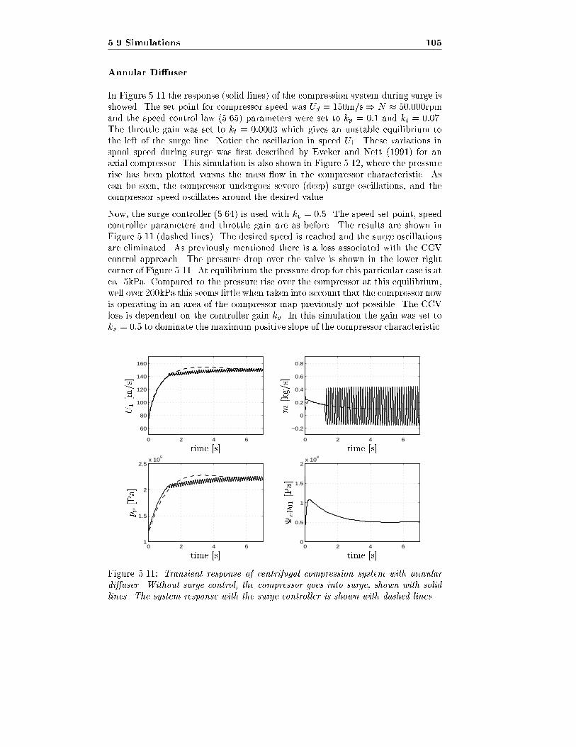
5.9 Simulations 105
Annular Di�user
In Figure 5.11 the response (solid lines) of the compression system during surge isshowed. The set point for compressor speed was Ud = 150m=s) N � 50:000rpmand the speed control law (5.65) parameters were set to kp = 0:1 and ki = 0:07.The throttle gain was set to kt = 0:0003 which gives an unstable equilibrium tothe left of the surge line. Notice the oscillation in speed U1. These variations inspool speed during surge was �rst described by Eveker and Nett (1991) for anaxial compressor. This simulation is also shown in Figure 5.12, where the pressurerise has been plotted versus the mass ow in the compressor characteristic. Ascan be seen, the compressor undergoes severe (deep) surge oscillations, and thecompressor speed oscillates around the desired value.
Now, the surge controller (5.64) is used with kv = 0:5. The speed set point, speedcontroller parameters and throttle gain are as before. The results are shown inFigure 5.11 (dashed lines). The desired speed is reached and the surge oscillationsare eliminated. As previously mentioned there is a loss associated with the CCVcontrol approach. The pressure drop over the valve is shown in the lower rightcorner of Figure 5.11. At equilibrium the pressure drop for this particular case is atca. 5kPa. Compared to the pressure rise over the compressor at this equilibrium,well over 200kPa this seems little when taken into account that the compressor nowis operating in an area of the compressor map previously not possible. The CCVloss is dependent on the controller gain kv. In this simulation the gain was set tokv = 0:5 to dominate the maximum positive slope of the compressor characteristic.
0 2 4 6
60
80
100
120
140
160
0 2 4 6
−0.2
0
0.2
0.4
0.6
0.8
0 2 4 61
1.5
2
2.5x 10
5
0 2 4 60
0.5
1
1.5
2x 10
4
m
[kg/s]
pp
[Pa]
U1[m/s]
time [s]time [s]
time [s]time [s]
vp01[Pa]
Figure 5.11: Transient response of centrifugal compression system with annular
di�user. Without surge control, the compressor goes into surge, shown with solid
lines. The system response with the surge controller is shown with dashed lines.
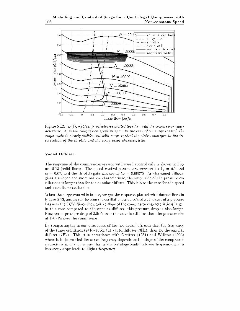
106
Modelling and Control of Surge for a Centrifugal Compressor with
Non-constant Speed
−0.2 −0.1 0 0.1 0.2 0.3 0.4 0.5 0.6 0.7 0.81
1.2
1.4
1.6
1.8
2
2.2
2.4
2.6
N = 20000
N = 30000
N = 35000
N = 40000
N = 45000
N = 50000
N = 55000
mass ow [kg/s]
pressurerisep(t)=p01
const. speed lines
surge line
throttle
stone wall
respns wo/control
respns w/control
Figure 5.12: (m(t); p(t)=p01)-trajectories plotted together with the compressor char-acteristic. N is the compressor speed in rpm. In the case of no surge control, the
surge cycle is clearly visible, but with surge control the state converges to the in-
tersection of the throttle and the compressor characteristic.
Vaned Di�user
The response of the compression system with speed control only is shown in Fig-ure 5.13 (solid lines). The speed control parameters were set to kp = 0:1 andki = 0:07, and the throttle gain was set at kT = 0:00075. As the vaned di�usergives a steeper and more narrow characteristic, the amplitude of the pressure os-cillations is larger than for the annular di�user. This is also the case for the speedand mass ow oscillations.
When the surge control is in use, we get the response plotted with dashed lines inFigure 5.13, and as can be seen the oscillations are avoided at the cost of a pressureloss over the CCV. Since the positive slope of the compressor characteristic is largerin this case compared to the annular di�user, this pressure drop is also larger.However, a pressure drop of 35kPa over the valve is still less than the pressure riseof 180kPa over the compressor.
By comparing the in-surge response of the two cases, it is seen that the frequencyof the surge oscillations is lower for the vaned di�user (3Hz), than for the annulardi�user (7Hz). This is in accordance with Greitzer (1981) and Willems (1996)where it is shown that the surge frequency depends on the slope of the compressorcharacteristic in such a way that a steeper slope leads to lower frequency, and aless steep slope leads to higher frequency.
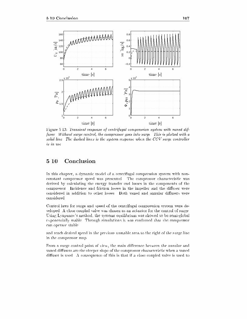
5.10 Conclusion 107
0 2 4 6
60
80
100
120
140
160
0 2 4 6
−0.2
0
0.2
0.4
0.6
0.8
0 2 4 61
1.5
2
2.5x 10
5
0 2 4 60
1
2
3
4
5x 10
4
m
[kg/s]
pp
[Pa]
vp01[Pa]
U1[m/s]
time [s]time [s]
time [s]time [s]
Figure 5.13: Transient response of centrifugal compression system with vaned dif-
fuser. Without surge control, the compressor goes into surge. This is plotted with a
solid line. The dashed lines is the system response when the CCV surge controller
is in use.
5.10 Conclusion
In this chapter, a dynamic model of a centrifugal compression system with non-constant compressor speed was presented. The compressor characteristic wasderived by calculating the energy transfer end losses in the components of thecompressor. Incidence and friction losses in the impeller and the di�user wereconsidered in addition to other losses. Both vaned and annular di�users wereconsidered.
Control laws for surge and speed of the centrifugal compression system were de-veloped. A close coupled valve was chosen as an actuator for the control of surge.Using Lyapunov's method, the systems equilibrium was showed to be semi-globalexponentially stable. Through simulations it was con�rmed that the compressorcan operate stable
and reach desired speed in the previous unstable area to the right of the surge linein the compressor map.
From a surge control point of view, the main di�erence between the annular andvaned di�users are the steeper slope of the compressor characteristic when a vaneddi�user is used. A consequence of this is that if a close coupled valve is used to

108
Modelling and Control of Surge for a Centrifugal Compressor with
Non-constant Speed
control surge, a greater pressure drop must be accepted over the valve in the caseof a vaned di�user than in the case of an annular di�user.
Chapter 6
Conclusions
In this thesis modeling and control of surge and rotating stall in axial and cen-trifugal compressors have been studied.
First, surge and stall controllers for a close coupled valve in series with a compressorwere developed. Using backstepping, a surge control law for the close coupled valvewas derived. Global asymptotic stability was proven. A more complicated surgecontrol law was derived for the case of both pressure disturbances and mass owdisturbances. Global uniform boundedness and convergence was proven. In orderto stabilize the compression system in the presence of constant disturbances, orbiases, in mass ow and pressure, an adaptive version of the surge controller wasderived. This controller ensures global asymptotic stability. Then, controllersfor rotating stall were considered. The close coupled valve was incooperated intothe Moore-Greitzer model, and controllers were derived that enables stabilizationof rotating stall beyond the surge line. Without disturbances, an asymptoticallystable equilibrium is ensured, and in the presence of pressure disturbances uniformboundedness was proven.
Then, the passivity properties of the Greitzer model was used to derive a surgecontrol law for a close coupled valve. This resulted in a simple proportional controllaw, that was capable of stabilizing the compression system in the presence of bothmass ow disturbances as well as pressure disturbances.
A multi mode Moore-Greitzer axial compressor model with spool dynamics wasderived. This resulted in a model with time varying B-parameter. Through sim-ulations it was demonstrated that the model was capable of demonstrating bothrotating stall and surge, and that the type of instability depended on the compres-sor speed. In the original Moore Greitzer model only the �rst mode of rotatingstall is included. The simulations in this chapter show that during stall inception,higher order modes can dominate the �rst mode. This is in accordance with knownresults, and is shown here to be valid also for variable speed compressors.
A dynamic model of a centrifugal compression system with non-constant compres-sor speed was presented. The compressor characteristic was derived by calculating
110 Conclusions
the energy transfer and losses in the components of the compressor. Incidence andfriction losses in the impeller and the di�user were considered in addition to otherlosses. Both vaned and annular di�users were considered. Control laws for surgeand speed of the centrifugal compression system were developed. A close cou-pled valve was chosen as an actuator for the control of surge. Using Lyapunov'smethod, the systems equilibrium was showed to be semi-global exponentially sta-ble. Through simulations it was con�rmed that the compressor can operate stableand reach desired speed in the previous unstable area to the right of the surge linein the compressor map.
Bibliography
Abed, E.H., P.K. Houpt and W.M. Hosny (1993). Bifurcation analysis of surge androtating stall in axial ow compressors. Journal of Turbomachinery 115, 817{824.
Adomatis, R.A. and E.H. Abed (1993). Local nonlinear control of stall inceptionin axial ow compressors. In: Proceedings of the AIAA/SAE/ASME/ASEE
Joint Propulsion Conference. Monterey, CA.
Badmus, O.O., S. Chowdhury and C.N. Nett (1996). Nonlinear control of surge inaxial compression systems. Automatica 32(1), 59{70.
Badmus, O.O., S. Chowdhury, K.M. Eveker and C.N. Nett (1995). Control-oriented high-frequency turbomachinery modelling: Single-stage compressionsystem one-dimensional modell. Journal of Turbomachinery 117, 47{61.
Balchen, J.G and K.I. Mumm�e (1988). Process control : Structures and applica-
tions. Van Nostrand Reinhold Company. New York.
Balj�e, O.E. (1952). A contribution to the problem of designing radial turboma-chines. Transactions of the ASME 74, 451{472.
Banaszuk, A., H.A. Hauksson and I. Mezi�c (1997). A backstepping controller fora partial di�erential equation model of compression system instabilities. In:Proceedings of the 36th Conference on Decision and Control. San Diego, CA.pp. 1050{1055.
Bazanella, A.S., P.V. Kokotovi�c and A.S. e Silva (1997). On the control of dynamicsystems with unknown operating point. In: Proceedings of the 1997 European
Control Conference. Brussels, Belgium.
Behnken, R.L. and R.M. Murray (1997). Combined air injection control of rotatingstall and bleed valve control of surge. In: Proceedings of the 1997 American
Control Conference. Albuquerque, NM.
Brown, D., L. Rachul and K. Williams (1997). NASA Researching Engine Air- ow Controls to Improve Performance, Fuel E�ciency. NASA press release,downloaded from Usenet newsgroup sci.space.news. Release: 97-183.
Cohen, H., G.F.C. Rogers and H.I.H Saravanamuttoo (1996). Gas turbine theory.4th ed.. Longman. Essex.
112 BIBLIOGRAPHY
Covert, E.E. (1995). Evolution of the commercial airliner. Scienti�c American
273(3), 82{85.
Cumpsty, N.A. (1989). Compressor Aerodynamics. Longman.
Day, I.J. (1993). Active suppression of rotating stall and surge in axial compressors.Journal of Turbomachinery 115, 40{47.
Day, I.J. (1994). Axial compressor performance during surge. Journal of propulsionand power 10(3), 329{336.
de Jager, B. (1995). Rotating stall and surge control : A survey. In: Proceedingsof the 35th Conference on Decision and Control. New Orleans, LA. pp. 1857{1862.
DeLaat, J.C., R.D. Southwick and G.W. Gallops (1996). High stability enginecontrol (HISTEC). In: Proceedings of AIAA/SAE/ASME/ASEE 32nd Joint
Propulsion Conference. Lake Buena Vista, FL. NASA TM 107272, AIAA-96-2586.
Dixon, S.L. (1978). Thermodynamics of turbomachinery. 3rd ed.. Pergamon Press.
Dussourd, J.L., G.W. Pfannebecker and S.K. Singhania (1976). Considerationsfor the control of surge in dynamic compressors using close coupled resis-tances. In: Centrifugal compressor and pump stability, stall and surge (P.C.Tramm and R.C. Dean, Jr., Eds.). pp. 1{28. ASME. New Orleans, Louisiana.Presented at the 1976 Joint gas turbine and uids engineering divisions' Con-ference.
Dussourd, J.L., G.W. Pfannebecker and S.K. Singhania (1977). An experimentalinvestigation of the control of surge in radial compressors using close coupledresistances. Journal of Fluids Engineering 99, 64{76.
Eastop, T.D. and A.McConkey (1986). Applied thermodynamics for engineering
technologists. 4th ed.. Longman. New York.
Emmons, H.W., C.E. Pearson and H.P. Grant (1955). Compressor surge and stallpropagation. Transactions of the ASME 77, 455{469.
Epstein, A.H., J.E. Ffowcs Williams and E.M. Greitzer (1989). Active suppres-sion of aerodynamic instabilities in turbomachines. Journal of Propulsion and
Power 5(2), 204{211.
Erskine, J.B. and N. Hensman (1975). Vibration induced by pump instability andsurging. In: Vibrations and noise in pump, fan, and compressor installations.The Institution of Mechanical Engineers. Mechanical Engineering Publica-tions limited. Southamton, UK. pp. 87{98.
Eveker, K.M. and C.N. Nett (1991). Model development for active surge controlrotating stall avoidance in aircraft gas turbine engines. In: Proceedings of the1991 American Control Conference. pp. 3166{3172.
BIBLIOGRAPHY 113
Ferguson, T.B. (1963). The centrifugal compressor stage. Butterworths. London.
Ffowcs Williams, J.E. and X.Y. Huang (1989). Active stabilization of compressorsurge. Journal of Fluid Mech. 204, 245{262.
Ffowcs Williams, J.E., M.F.L. Harper and D.J. Allwright (1993). Active stabi-lization of compressor instability and surge in a working engine. Journal ofTurbomachinery 115, 68{75.
Fink, D.A., N.A. Cumpsty and E.M. Greitzer (1992). Surge dynamics in a free-spool centrifugal compressor system. Journal of Turbomachinery 114, 321{332.
Godhavn, J.-M. (1997). Topics in nonlinear motion control: nonholonomic, under-actuated and hybrid systems. PhD thesis. Norwegian University of Scienceand Technology. Dept of Engineering Cybernetics.
Gravdahl, J.T. (1998). Modeling and Close Coupled Valve Control of Compressor
Surge and Rotating Stall. Advances in Industrial Control. Springer-Verlag.London. Accepted for publication, to appear.
Gravdahl, J.T. and O. Egeland (1997a). A Moore-Greitzer axial compressor modelwith spool dynamics. In: Proceedings of the 36th IEEE Conference on Deci-
sion and Control. San Diego, CA. pp. 4714{4719.
Gravdahl, J.T. and O. Egeland (1997b). Centrifugal compressor surge and speedcontrol. Submitted to IEEE Transactions on Control Systems Technology.
Gravdahl, J.T. and O. Egeland (1997c). Compressor surge control using a close-coupled valve and backstepping. In: Proceedings of the 1997 American Control
Conference. Albuquerque, NM.
Gravdahl, J.T. and O. Egeland (1997d). Control of the three-state Moore-Greitzercompressor model using a close-coupled valve. In: Proceedings of the 1997
European Control Conference. Brussels, Belgium.
Gravdahl, J.T. and O. Egeland (1997e). Modeling of rotating stall and surge in afree spool axial compression system. Submitted to Journal of Turbomachinery.
Gravdahl, J.T. and O. Egeland (1997f). Passivity based compressor surge controlusing a close-coupled valve. In: Proceedings of the 1997 COSY Workshop
on Control of Nonlinear and Uncertain Systems (A. Isidori and F. Allg�ower,Eds.). Zurich, Switzerland. pp. 139{143.
Gravdahl, J.T. and O. Egeland (1997g). Speed and surge control for a low or-der centrifugal compressor model. In: Proceedings of the 1997 International
Conference on Control Applications. Hartford, CT. pp. 344{349.
Gravdahl, J.T. and O. Egeland (1998a). Close Coupled Valve control of surge androtating stall in compressors. Submitted to Automatica.
114 BIBLIOGRAPHY
Gravdahl, J.T. and O. Egeland (1998b). Speed and surge control for a low ordercentrifugal compressor model.Modeling, Identi�cation and Control 19(1), 13{29.
Gravdahl, J.T. and O. Egeland (1998c). Two results on compressor surge con-trol with disturbance rejection. Submitted to the 37th IEEE Conference onDecision and Control.
Greitzer, E.M. (1976a). Surge and Rotating stall in axial ow compressors, PartI: Theoretical compression system model. Journal of Engineering for Power
98, 190{198.
Greitzer, E.M. (1976b). Surge and rotating stall in axial ow compressors, PartII: Experimental results and comparison with theory. Journal of Engineeringfor Power 98, 199{217.
Greitzer, E.M. (1977). Coupled compressor-di�user ow instability. Journal ofaircraft 14(3), 233{238.
Greitzer, E.M. (1980). REVIEW{Axial compressor stall phenomena. Journal ofFluids Engineering 102, 134{151.
Greitzer, E.M. (1981). The stability of pumping systems { The 1980 Freemanscholar lecture. Journal of Fluids Engineering 103, 193{242.
Greitzer, E.M. and F.K. Moore (1986). A theory of post-stall transients in a axialcompressor systems: Part II{Application. Journal of Engineering for Gas
Turbines and Power 108, 231{239.
Greitzer, E.M. and H.R. Griswold (1976). Compressor-di�user interaction withcircumferential ow distortion. The journal of mechanical engineering science18(1), 25{43.
Gu, G., S. Banda and A. Sparks (1996). An overview of rotating stall and surgecontrol for axial ow compressors. In: Proceedings of the 35th Conference on
Decision and Control. Kobe, Japan.
Gysling, D.L., J. Dugundji, E.M. Greitzer and A.H. Epstein (1991). Dynamiccontrol of centrifugal compressors surge using tailored structures. Journal ofTurbomachinery 113, 710{722.
Haddad, W.M., J.L. Fausz, V.-S. Chellaboina and A. Leonessa (1997). Nonlinearrobust disturbance rejection controllers for rotating stall and surge in axial ow compressors. In: Proceedings of the 1997 International Conference on
Control Applications. Hartford, CT. pp. 767{772.
Hansen, K.E., P. J�rgensen and P.S. Larsen (1981). Experimental and theoreticalstudy of surge in a small centrifugal compressor. Journal of Fluids Engineering103, 391{394.
Hendricks, G.J. and D.L. Gysling (1994). Theoretical study of sensor-actuatorschemes for rotating stall control. Journal of Propulsion and Power
10(1), 101{109.
BIBLIOGRAPHY 115
Hendrickson, E.S. and A.G. Sparks (1997). On the suitability of bifurcation sta-bilization control laws for high order Moore-Greitzer compressor models. In:Proceedings of the 1997 American Control Conference. Albuquerque, NM.
Horlock, J.H. (1958). Axial ow compressors: Fluid mechanics and Thermody-
namics. Butterworths scienti�c publications. London.
Humbert, J.S. and A.J. Krener (1997). Analysis of higher order Moore-Greitzercompressor models. In: Proceedings of the 1997 International Conference on
Control Applications. Hartford, CT. pp. 651{656.
Hynes, J.M., G.J. Hendricks and A.H. Epstein (1994). Active stabilization of ro-tating stall in a three-stage axial compressor. Journal of Turbomachinery116, 226{239.
Hynes, T.P. and E.M. Greitzer (1987). A method for assessing e�ects of circum-ferential ow distortion on compressor stability. Journal of Turbomachinery109, 371{379.
Johnston, J.P. and R.C. Dean, Jr. (1966). Losses in vaneless di�users of centrifugalcompressors and pumps. Analysis, experiment and design. Journal of Engi-neering for Power pp. 49{62.
Jungowski, W.M., M.H. Weiss and G.R. Price (1996). Pressure oscillations occur-ring in a centrifugal compressor system with and without passive and activesurge control. Journal of Turbomachinery 118, 29{40.
Ko�, S.G. and E.M. Greitzer (1986). Axisymmetrically stalled ow performancefor multistage axial compressors. Journal of Turbomachinery 108, 216{249.
Krsti�c, M. (1996). Invariant manifolds and asymptotic properties of adaptive non-linear stabilizers. IEEE Transactions on automatic control 41(6), 817{829.
Krsti�c, M. and P.V. Kokotovi�c (1995). Lean backstepping designs for jet enginecompressor model. In: Proceedings of the 4th IEEE Conference on Control
Applications. pp. 1047{1052.
Krsti�c, M., I. Kanellakopoulos and P.V. Kokotovi�c (1995a). Nonlinear and Adap-
tive Control Design. John Wiley & Sons Inc.
Krsti�c, M., J.M. Protz, J.D. Paduano and P.V. Kokotovi�c (1995b). Backsteppingdesigns for jet engine stall and surge control. In: Proceedings of the 35th
Conference on Decision and Control. New Orleans, LA. pp. 3049{3055.
Leonessa, A., V.-S. Chellaboina and W.M. Haddad (1997a). Globally stabiliz-ing controllers for multi-mode axial ow compressor models via equilibria-dependent lyapunov functions. In: Proceedings of the 1997 International Con-ference on Control Applications. Hartford, CT. pp. 63{68.
Leonessa, A., V.-S. Chellaboina and W.M. Haddad (1997b). Robust stabilizationof axial ow compressors with uncertain pressure- ow maps. In: Proceedingsof the 1997 International Conference on Control Applications. Hartford, CT.pp. 671{676.
116 BIBLIOGRAPHY
Liaw, D.-C. and E.H. Abed (1992). Stability analysis and control of rotating stall.In: Proceedings of NOLCOS'92: Nonlinear Control System Design Sympo-
sium (M. Fliess, Ed.). Bourdaux, France. pp. 88{93.
Liaw, D.-C. and E.H. Abed (1996). Active control of compressor stall inception: abifurcation-theoretic approach. Automatica 32(1), 109{115.
Lorett, J.A. and S. Gopalakrishnan (1986). Interaction between impeller and vo-lute of pumps at o�-design conditions. Journal of uids engineering 108, 12{18.
Mansoux, C.A., D.L. Gysling, J.D. Setiawan and J.D. Paduano (1994). Distributednonlinear modeling and stability analysis of axial compressor stall and surge.In: Proceedings of the 1994 American Control Conference. Baltimore, Mary-land. pp. 2305{2316.
Mattingly, J.D. (1996). Elements of gas turbine propulsion. McGraw-Hill series inaeronautical and aerospace engineering. McGraw-Hill.
McCaughan, F.E. (1989). Application of Bifurcation theory to axial ow compres-sor instability. Journal of Turbomachinery 111, 426{433.
Moore, F.K. (1984a). A theory of rotating stall of multistage axial compres-sors: Part I{Small disturbances. Journal of Engineering for Gas Turbines
and Power 106, 313{320.
Moore, F.K. (1984b). A theory of rotating stall of multistage axial compressors:Parts I,II,III. J. of Engineering for Gas Turbines and Power 106, 313{336.
Moore, F.K. and E.M. Greitzer (1986). A theory of post-stall transients in a axialcompressor systems: Part I{Development of equations. Journal of Engineer-ing for Gas Turbines and Power 108, 68{76.
Murray, S. Yeung R.M. (1997). Reduction of bleed valve rate requirements forcontrol of rotating stall using continuous air injection. In: Proceedings of
the 1997 International Conference on Control Applications. Hartford, CT.pp. 683{690.
Nicklasson, P.J. (1996). Passivity-based control of electric machines. PhD thesis.Norwegian Institute of Technology. Dept of Engineering Cybernetics.
Nisenfeld, A.E. (1982). Centrifugal compressors: principles of operation and con-
trol. Instrument society of America.
Osborn, W.M. and J.M. Wagner (1970). E�ect of simulated downstream owblockage doors on the performance of an axial- ow fan rotor. Technical ReportTN D-6071. NASA.
Paduano, J.D., A.H. Epstein, L. Valavani, J.P. Longley, E.M. Greitzer and G.R.Guenette (1993). Active control of rotating stall in a low-speed axial com-pressor. Journal of Turbomachinery 115, 48{56.
BIBLIOGRAPHY 117
Paduano, J.D., A.H. Epstein, L. Valavani, J.P. Longley, E.M. Greitzer andG.R. Guenette (1995). Modelling for control of rotating stall. Automatica30(9), 1357{1373.
Pampreen, R.C. (1973). Small turbomachinery compressor and fan aerodynamics.Journal of engineering for power 95, 251{256.
Perko, L. (1991). Di�erential equations and dynamical systems. Vol. 7 of Texts inApplied Mathematics. Springer-Verlag.
Pinsley, J.E., G.R. Guenette, A.H. Epstein and E.M. Greitzer (1991). Active stabi-lization of centrifugal compressor surge. Journal of Turbomachinery 113, 723{732.
Protz, J.M. and J.D. Paduano (1997). Rotating stall and surge: Alternate model-ing and control concepts. In: Proceedings of the 1997 International Conferenceon Control Applications. Hartford, CT. pp. 866{873.
Ru�es, P.C (1996). Innovation in aero engines. The Aeronautical Journal
100(1000), 473{484.
Sepulchre, R. and P. Kokotovi�c (1996). Shape signi�ers for throttle control of alow-order compressor model.
Simon, J.S. and L. Valavani (1991). A Lyapunov based nonlinear control schemefor stabilizing a basic compression system using a close-coupled control valve.In: Proceedings of the 1991 American Control Conference. pp. 2398{2406.
Simon, J.S., L. Valavani, A.H. Epstein and E.M. Greitzer (1993). Evaluation of ap-proaches to active compressor surge stabilization. Journal of Turbomachinery115, 57{67.
Simon, S. (1993). Feedback stabilization of compression systems. PhD thesis. MIT.
Stenning, A.H. (1980). Rotating stall and surge. Journal of uids engineering
102, 14{21.
van de Wal, M. and F. Willems (1996). Selection of actuators and sensors forcompressor control. Technical Report WFW 96.155. Eindhoven University ofTechnology.
van de Wal, M., F. Willems and B. de Jager (1997). Selection of actuators andsensors for active surge control. In: Proceedings of the 1997 International
Conference on Control Applications. Hartford, CT. pp. 121{127.
van der Schaft, A.J. (1996). L2-gain and passivity techniques in nonlinear con-
trol. Vol. 218 of Lecture notes in Control and Information Sciences. Springer-Verlag. Heidelberg.
Wang, H.-H. and M. Krsti�c (1997a). Control of Deep-Hysteresis aeroenginecompressors{Part I : A Moore-Greitzer type model. In: Proceedings of the
1997 American Control Conference. Albuquerque, NM.
118 BIBLIOGRAPHY
Wang, H.-H. and M. Krsti�c (1997b). Control of deep hysteresis compressors un-der limited actuator bandwidth. In: Proceedings of the 1997 International
Conference on Control Applications. Hartford, CT. pp. 657{662.
Watson, N. and M.S. Janota (1982). Turbocharging the internal combustion engine.MacMillan.
Weigl, H.J. and J.D. Paduano (1997). Application of H1 control with eigenvalueperturbations to stabilize a transonic compressor. In: Proceedings of the 1997International Conference on Control Applications. Hartford, CT. pp. 691{698.
White, F.M. (1986). Fluid mechanics. 2nd ed.. McGraw-Hill. New York.
Whit�eld, A. and F.J. Wallace (1973). Study of incidence loss models in radialand mixed- ow turbomachinery. In: Proceedings of the conference on heat
and uid ow in steam and gas turbine plant. The instn. of Mech. Engnrs..U. of Warwick, Coventry. pp. 122{128.
Whit�eld, A. and F.J. Wallace (1975). Performance prediction for automotive tur-bocharger compressors. Proceedings of the institution of mechanical engineers
189(12), 59{67.
Willems, F. (1996). Modeling and control of compressor ow instabilities. TechnicalReport WFW 96.151. Eindhoven University of Technology.
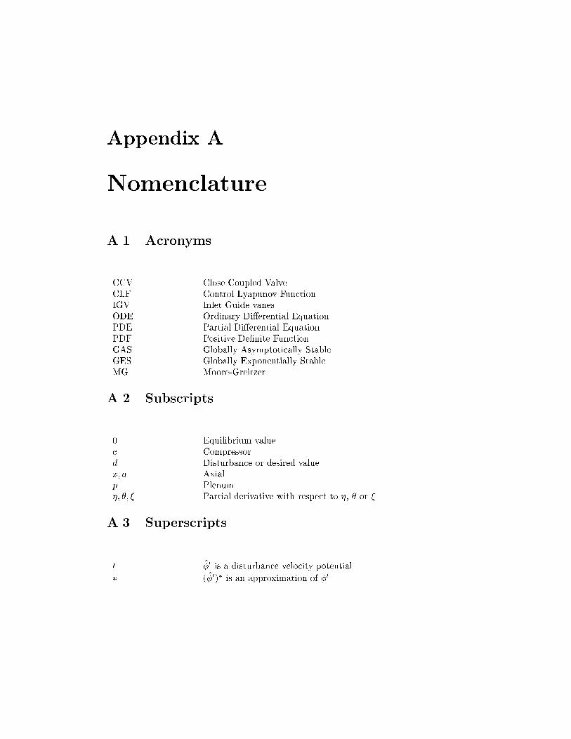
Appendix A
Nomenclature
A.1 Acronyms
CCV Close Coupled ValveCLF Control Lyapunov FunctionIGV Inlet Guide vanesODE Ordinary Di�erential EquationPDE Partial Di�erential EquationPDF Positive De�nite FunctionGAS Globally Asymptotically StableGES Globally Exponentially StableMG Moore-Greitzer
A.2 Subscripts
0 Equilibrium valuec Compressord Disturbance or desired valuex; a Axialp Plenum�; �; � Partial derivative with respect to �, � or �
A.3 Superscripts
0 �0 is a disturbance velocity potential
� (�0)� is an approximation of �0
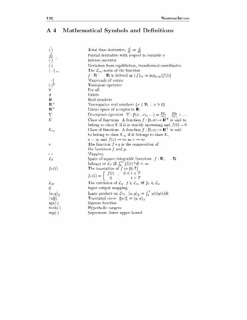
120 Nomenclature
A.4 Mathematical Symbols and De�nitions
_(�) Total time derivative, d
dtor d
d�
@
@xPartial derivative with respect to variable x
(�)�1 Inverse operator
(�) Deviation from equilibrium, transformed coordinatesk � k1 The L1-norm of the function
f : IIR+ ! IIR is de�ned as kfk1 = supt�0 jf(t)j
j � j Magnitude of vector(�)T Transpose operator8 For all9 ExistsIIR Real numbers
IIR+ Nonnegative real numbers fx 2 IIR : x � 0gIIRn Linear space of n-tuples in IIR
r Divergence operator. r � f(x1; x2; : : :) = @f1
@x1+ @f2
@x2+ : : :
K Class of functions. A function f : [0; a)! IIR+ is said tobelong to class K if it is strictly increasing and f(0) = 0.
K1 Class of functions. A function f : [0; a)! IIR+ is saidto belong to class K1 if it belongs to class K,a =1 and f(r)!1 as r !1.
� The function f � g is the composition ofthe functions f and g
7! MappingL2 Space of square integrable functions. f : IIR+ ! IIR
belongs to L2 i�R10jf(t)j2dt <1
fT (t) The truncation of f to [0; T ].
fT (t) =
�f(t) ; 0 � t < T
0 ; t � T
L2e The extension of L2. f 2 L2e i� fT 2 L2G Input-output mapping
hu; yiT
Inner product on L2e. hu; yiT =RT
0u(t)y(t)dt
kuk2T
Truncated norm. kuk2T= hu; ui
T
sgn(�) Signum functiontanh(�) Hyperbolic tangentsup(�) Supremum, lower upper bound
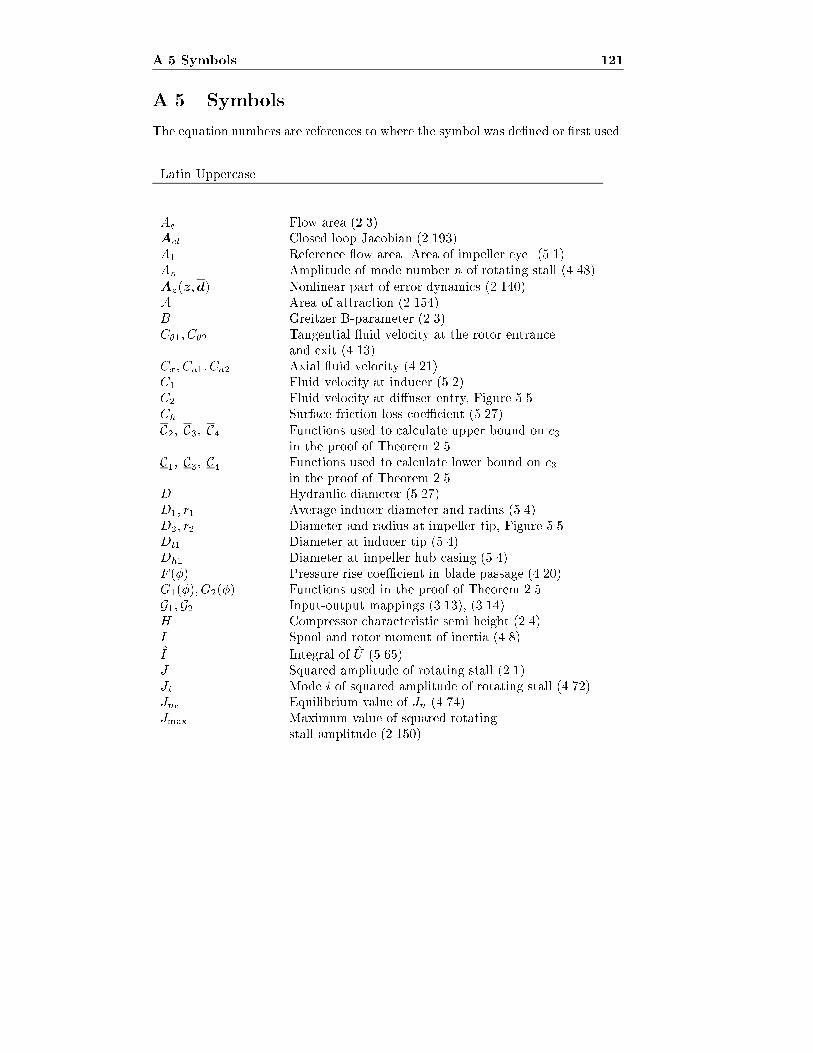
A.5 Symbols 121
A.5 Symbols
The equation numbers are references to where the symbol was de�ned or �rst used.
Latin Uppercase
Ac Flow area (2.3)Acl Closed loop Jacobian (2.193)A1 Reference ow area. Area of impeller eye. (5.1)An Amplitude of mode number n of rotating stall (4.48)
Az(z;d) Nonlinear part of error dynamics (2.140)A Area of attraction (2.154)B Greitzer B-parameter (2.3)C�1; C�2 Tangential uid velocity at the rotor entrance
and exit (4.13)Cx; Ca1; Ca2 Axial uid velocity (4.21)C1 Fluid velocity at inducer (5.2)C2 Fluid velocity at di�user entry, Figure 5.5Ch Surface friction loss coe�cient (5.27)
C2; C3; C4 Functions used to calculate upper bound on c3in the proof of Theorem 2.5
C1; C3; C4 Functions used to calculate lower bound on c3in the proof of Theorem 2.5
D Hydraulic diameter (5.27)D1; r1 Average inducer diameter and radius (5.4)D2; r2 Diameter and radius at impeller tip, Figure 5.5Dt1 Diameter at inducer tip (5.4)Dh1 Diameter at impeller hub casing (5.4)F (�) Pressure rise coe�cient in blade passage (4.20)G1(�); G2(�) Functions used in the proof of Theorem 2.5G1;G2 Input-output mappings (3.13), (3.14)H Compressor characteristic semi height (2.4)I Spool and rotor moment of inertia (4.8)
I Integral of U (5.65)J Squared amplitude of rotating stall (2.1)Ji Mode i of squared amplitude of rotating stall (4.72)Jne Equilibrium value of Jn (4.74)Jmax Maximum value of squared rotating
stall amplitude (2.150)
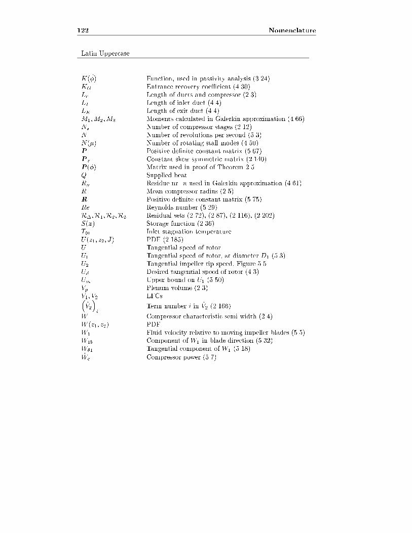
122 Nomenclature
Latin Uppercase
K(�) Function, used in passivity analysis (3.24)KG Entrance recovery coe�cient (4.30)Lc Length of ducts and compressor (2.3)LI Length of inlet duct (4.4)LE Length of exit duct (4.4)M1;M2;M3 Moments calculated in Galerkin approximation (4.66)Ns Number of compressor stages (2.12)N Number of revolutions per second (5.3)N(�) Number of rotating stall modes (4.50)P Positive de�nite constant matrix (5.67)P z Constant skew symmetric matrix (2.140)P (�) Matrix used in proof of Theorem 2.5Q Supplied heatRn Residue nr. n used in Galerkin approximation (4.61)R Mean compressor radius (2.5)R Positive de�nite constant matrix (5.75)Re Reynolds number (5.29)R�;R1;R2;R3 Residual sets (2.72), (2.87), (2.116), (2.202)S(z) Storage function (2.36)T01 Inlet stagnation temperatureU(z1; z2; J) PDF (2.185)U Tangential speed of rotorU1 Tangential speed of rotor, at diameter D1 (5.3)U2 Tangential impeller tip speed, Figure 5.5Ud Desired tangential speed of rotor (4.3)Um Upper bound on U1 (5.50)Vp Plenum volume (2.3)V1; V2 LFCs�_V2
�i
Term number i in _V2 (2.166)
W Compressor characteristic semi width (2.4)W (z1; z2) PDFW1 Fluid velocity relative to moving impeller blades (5.5)W1b Component of W1 in blade direction (5.32)W�1 Tangential component of W1 (5.18)_Wc Compressor power (5.7)
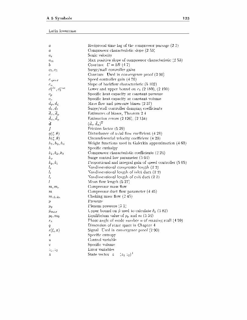
A.5 Symbols 123
Latin lowercase
a Reciprocal time lag of the compressor passage (2.2)a Compressor characteristic slope (2.53)as Sonic velocityam Max positive slope of compressor characteristic (2.53)b Constant. U = bB (4.7)c2; c3 Surge/stall controller gainsc Constant. Used in convergence proof (2.90)cspeed Speed controller gain (4.76)cn Slope of back ow characteristic (5.102)cmin3 ; cmax3 Lower and upper bound on c3 (2.189), (2.190)cp Speci�c heat capacity at constant pressurecv Speci�c heat capacity at constant volumed�; d Mass ow and pressure biases (2.37)d1; d2 Surge/stall controller damping coe�cients
d ; d� Estimates of biases, Theorem 2.4~d ; ~d� Estimation errors (2.126), (2.134)~d ( ~d ~d�)
T
f Friction factor (5.29)g(�; �) Disturbance of axial ow coe�cient (4.28)h(�; �) Circumferential velocity coe�cient (4.28)h1; h2; h3 Weight functions used in Galerkin approximation (4.63)h Speci�c enthalpyk1; k2; k3 Compressor characteristic coe�cients (2.24)kv Surge control law parameter (5.64)kp; ki Proportional and integral gain of speed controller (5.65)lc Nondimensional compressor length (2.2)li Nondimensional length of inlet duct (2.2)le Nondimensional length of exit duct (2.2)l Mean ow length (5.27)m;mc Compressor mass owm Compressor duct ow parameter (4.45)mchoke Choking mass ow (2.45)p Pressurepp Plenum pressure (5.1)pmax Upper bound on p used to calculate �2 (5.82)p0;m0 Equilibrium value of pp and m (5.54)rn Phase angle of mode number n of rotating stall (4.59)q Dimension of state space in Chapter 4s(�; z) Signal. Used in convergence proof (2.90)s Speci�c entropyu Control variablev Speci�c volumez1; z2 Error variablesz State vector. z = (z1 z2)
T
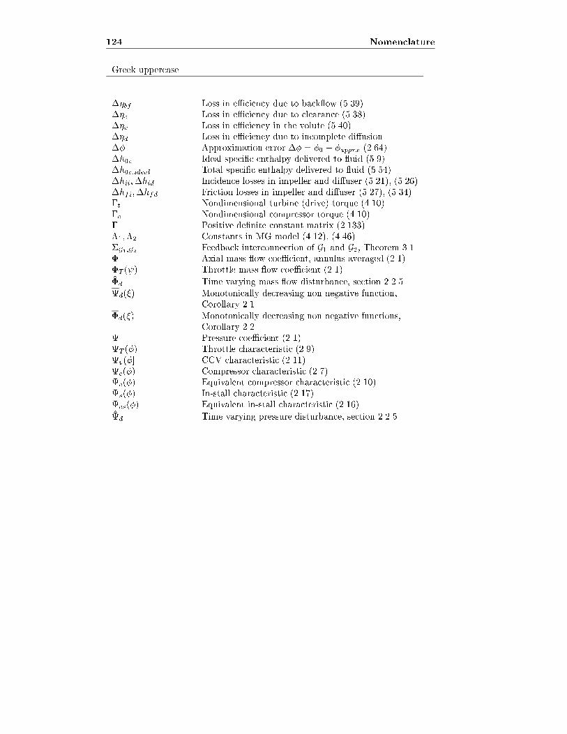
124 Nomenclature
Greek uppercase
��bf Loss in e�ciency due to back ow (5.39)��c Loss in e�ciency due to clearance (5.38)��v Loss in e�ciency in the volute (5.40)��d Loss in e�ciency due to incomplete di�usion�� Approximation error �� = �0 � �apprx (2.64)�h0c Ideal speci�c enthalpy delivered to uid (5.9)�h0c;ideal Total speci�c enthalpy delivered to uid (5.54)�hii;�hid Incidence losses in impeller and di�user (5.21), (5.26)�hfi;�hfd Friction losses in impeller and di�user (5.27), (5.34)�t Nondimensional turbine (drive) torque (4.10)�c Nondimensional compressor torque (4.10)� Positive de�nite constant matrix (2.133)�1;�2 Constants in MG model (4.12), (4.46)�G1;G2 Feedback interconnection of G1 and G2, Theorem 3.1� Axial mass ow coe�cient, annulus averaged (2.1)�T ( ) Throttle mass ow coe�cient (2.1)
�d Time varying mass ow disturbance, section 2.2.5
d(�) Monotonically decreasing non negative function,Corollary 2.1
�d(�) Monotonically decreasing non negative functions,Corollary 2.2
Pressure coe�cient (2.1)T (�) Throttle characteristic (2.9)v(�] CCV characteristic (2.11)c(�) Compressor characteristic (2.7)e(�) Equivalent compressor characteristic (2.10)s(�) In-stall characteristic (2.17)es(�) Equivalent in-stall characteristic (2.16)
d Time varying pressure disturbance, section 2.2.5
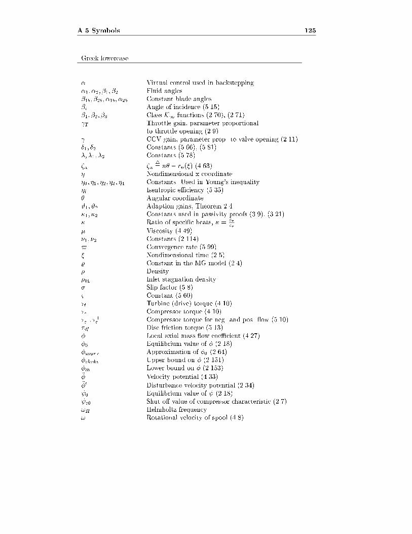
A.5 Symbols 125
Greek lowercase
� Virtual control used in backstepping�1; �2; �1; �2 Fluid angles�1b; �2b; �1b; �2b Constant blade angles�i Angle of incidence (5.15)�1; �2; �3 Class K1 functions (2.70), (2.71) T Throttle gain, parameter proportional
to throttle opening (2.9) CCV gain, parameter prop. to valve opening (2.11)�1; �2 Constants (5.66), (5.81)�; �1; �2 Constants (5.78)
�n �n4= n� � rn(�) (4.63)
� Nondimensional x-coordinate�0; �1; �2; �3; �4 Constants. Used in Young's inequality�i Isentropic e�ciency (5.35)� Angular coordinate#1; #2 Adaption gains, Theorem 2.4�1; �2 Constants used in passivity proofs (3.9), (3.21)� Ratio of speci�c heats, � =
cp
cv
� Viscosity (4.49)�1; �2 Constants (2.114)$ Convergence rate (5.99)� Nondimensional time (2.5)% Constant in the MG model (2.4)� Density�01 Inlet stagnation density� Slip factor (5.8)& Constant (5.60)�t Turbine (drive) torque (4.10)�c Compressor torque (4.10)��c; �+c
Compressor torque for neg. and pos. ow (5.10)�df Disc friction torque (5.13)� Local axial mass ow coe�cient (4.27)�0 Equilibrium value of � (2.18)�apprx Approximation of �0 (2.64)�choke Upper bound on � (2.151)�m Lower bound on � (2.153)~� Velocity potential (4.33)~�0 Disturbance velocity potential (2.34) 0 Equilibrium value of (2.18) c0 Shut o� value of compressor characteristic (2.7)!H Helmholtz frequency! Rotational velocity of spool (4.8)

126 Nomenclature
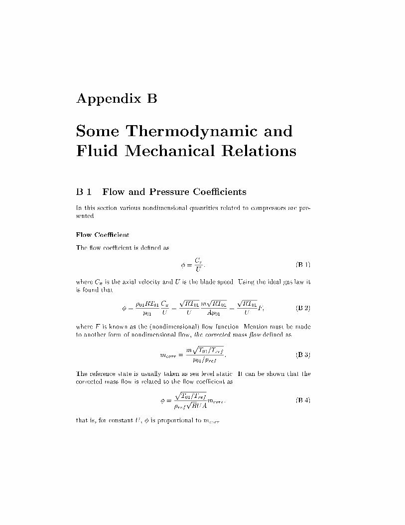
Appendix B
Some Thermodynamic and
Fluid Mechanical Relations
B.1 Flow and Pressure Coe�cients
In this section various nondimensional quantities related to compressors are pre-sented.
Flow Coe�cient
The ow coe�cient is de�ned as
� =Cx
U; (B.1)
where Cx is the axial velocity and U is the blade speed. Using the ideal gas law itis found that
� =�01RT01
p01
Cx
U=
pRT01
U
mpRT01
Ap01=
pRT01
UF; (B.2)
where F is known as the (nondimensional) ow function. Mention must be madeto another form of nondimensional ow, the corrected mass ow de�ned as
mcorr =mpT01=Tref
p01=pref: (B.3)
The reference state is usually taken as sea level static. It can be shown that thecorrected mass ow is related to the ow coe�cient as
� =
pT01=Tref
�refpRUA
mcorr; (B.4)
that is, for constant U , � is proportional to mcorr.
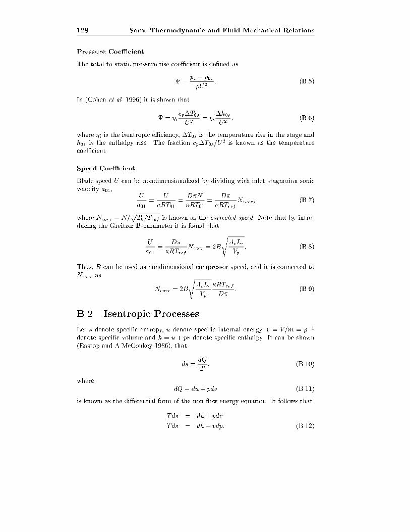
128 Some Thermodynamic and Fluid Mechanical Relations
Pressure Coe�cient
The total to static pressure rise coe�cient is de�ned as
=p1 � p01
�U2: (B.5)
In (Cohen et al. 1996) it is shown that
= �icp�T0sU2
= �i�h0sU2
; (B.6)
where �i is the isentropic e�ciency, �T0s is the temperature rise in the stage andh0s is the enthalpy rise. The fraction cp�T0s=U
2 is known as the temperaturecoe�cient.
Speed Coe�cient
Blade speed U can be nondimensionalized by dividing with inlet stagnation sonicvelocity a01,
U
a01=
U
�RT01=
D�N
�RT01=
D�
�RTrefNcorr; (B.7)
where Ncorr = N=pT0=Tref is known as the corrected speed. Note that by intro-
ducing the Greitzer B-parameter it is found that
U
a01=
D�
�RTrefNcorr = 2B
sAcLc
Vp: (B.8)
Thus, B can be used as nondimensional compressor speed, and it is connected toNcorr as
Ncorr = 2B
sAcLc
Vp
�RTref
D�: (B.9)
B.2 Isentropic Processes
Let s denote speci�c entropy, u denote speci�c internal energy, v = V=m = ��1
denote speci�c volume and h = u+ pv denote speci�c enthalpy. It can be shown(Eastop and A.McConkey 1986), that
ds =dQ
T; (B.10)
wheredQ = du+ pdv (B.11)
is known as the di�erential form of the non- ow energy equation. It follows that
Tds = du+ pdv
Tds = dh� vdp: (B.12)
B.3 Mass Balance of the Plenum 129
With constant speci�c heat capacities cp and cv,
Tds = cvdT + pdv
Tds = cpdT � vdp: (B.13)
For isentropic processes, that is reversible and adiabatic, ds = 0, and accordingly
dT = � p
cvdv
dT =v
cpdp; (B.14)
which in turn impliesdp
p= ��dv
v; (B.15)
where � =cp
cvis the ratio of speci�c heats.
B.3 Mass Balance of the Plenum
The plenum process is assumed to be isentropic, which means that the di�erentialform (B.15) of the isentropic relation is valid, so that
dpp
pp= ��dvp
vp= �
d�p
�p; (B.16)
where it has been used that
� =1
v) d�
�= �dv
v: (B.17)
It follows that_pp =
�pp
�p_�p = �RTp _�p: (B.18)
The mass balance of the plenum is
_�p =1
Vp(m�mt); (B.19)
and it follows that
_pp =�RTp
Vp(m�mt) =
a2s
Vp(m�mt); (B.20)
where as =p�RTp is the plenum sonic velocity. As velocities in the plenum are
assumed negligible, a0 can be used in (B.20). The sound speed in the plenum willwary as both temperature and pressure in the plenum varies with time. In (Simonet al. 1993), a time mean speed of sound in the plenum, as was used. Anotherapproach to avoid using the plenum sonic velocity was taken in (Greitzer 1976a).It was recognized that by assuming that the temperature ratios of the compressionsystem are near unity, the quantity �p=pp = RTp is not appreciably di�erent from�01=p01. Thus, the speed of sound at ambient conditions can be used in (B.20).This approach is also taken in this thesis.
130 Some Thermodynamic and Fluid Mechanical Relations
B.4 Flow through a Nozzle
The stagnation temperature is
T0 = T +1
2cpC2x; (B.21)
where T is the static temperature and Cx is the velocity of the ow. The Machnumber is
M =Cx
as; (B.22)
whereas =
p�RT; (B.23)
is the sonic velocity. Then C2x=M2�RT and it follows that
T0
T= 1 +
M2�R
2cp= 1 +
�� 1
2M2: (B.24)
Using the isentropic relation
T0
T=
�p
p0
� (��1)
�
; (B.25)
it is found thatp0
p=
�1 +
�� 1
2M2
� �
��1
: (B.26)
The mass ow ism = �ACx; (B.27)
where A is the ow crossectional area. Alternative forms are
m = �AMas = A�p�RTM = A
ppRT
p�M
= Ap0pRT0
p
p0
rT0
T
p�M; (B.28)
where it is used that � = p=RT . Then, by the use of (B.25) and (B.26), it is foundthat
m = Ap0pRT0
p�M
�1 +
�� 1
2M2
�� �+1
2(��1)
: (B.29)
The critical mass ow, or choked ow, is found by inserting M = 1 and using theideal gas law in the form RT0 = �0=p0. This gives
mchoke = Ap��0p0
�2
�+ 1
� �+1
2(��1)
(B.30)
= A�0a0
�2
�+ 1
� �+1
2(��1)
: (B.31)
B.5 Compressor Pressure Rise 131
B.5 Compressor Pressure Rise
Here equation (5.42) for the compressor pressure rise is derived. The compressortotal to static isentropic e�ciency can be written
�i(m;U1) =h2s � h01
h02 � h01; (B.32)
where h2s is the outlet static enthalpy obtained with isentropic compression, h01is the inlet stagnation, or total, enthalpy and h02 is the outlet stagnation, or total,enthalpy.Considering a perfect gas, we have that h = Tcp, where cp is the speci�c heatcapacity at constant pressure. For a perfect gas, cp is constant. The e�ciencynow is
�i(m;U1) =T2s � T01
T02 � T01=
T2s
T01� 1
T02
T01� 1
: (B.33)
Using the relation for isentropic compression (B.25),
�i(m;U1) =
�p2
p01
���1� � 1
T02
T01� 1
=
T01cp
��p2
p01
���1� � 1
�cp(T02 � T01)
: (B.34)
For a radially vaned impeller (Watson and Janota 1982):
�i(m;U1) =
T01cp
��p2
p01
���1� � 1
��h0c;ideal
; (B.35)
which can be rearranged to
p2
p01=
�1 +
�i(m;U1)�h0c;idealT01cp
� �
��1
: (B.36)

132 Some Thermodynamic and Fluid Mechanical Relations
Appendix C
Including a Close Coupled
Valve in the Moore-Greitzer
Model
Equation numbers starting with MG are references to the paper Moore and Gre-itzer (1986).Equation (MG5), which gives the pressure rise over the compressor is modi�ed to
pE � p1
�U2= NsF (�)� 1
2a
�2@�
@�+@�
@�
�| {z }
Equation (5) in Moore and Greitzer (1986)
�v(�); (C.1)
where v(�) is the pressure drop across the CCV, and pE now is the pressure atthe exit of the CCV. Using equation (MG23), the pressure rise over the equivalentcompressor is written
e(�) = NsF (�) � 1
2�2| {z }
c(�)
�v(�): (C.2)
Using this, the local (in �) and annulus averaged momentum balances (equations(MG42) and (MG43)), are modi�ed to
(�) + lcd�
d�= c(�� Y��)� v(�� Y��)�mY� +
1
2a(2Y��� + Y���) (C.3)
and
(�) + lcd�
d�=
1
2�
Z 2�
0
f c(�� Y��)� v(�� Y��)g d�: (C.4)
In the case of pure surge, that is Y � 0, the two momentum balances are the sameand is reduced to
_� =1
lc(c(�)�v(�)�); (C.5)
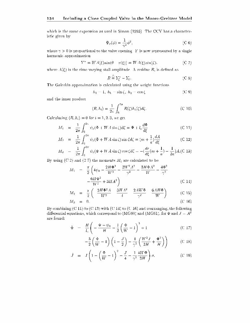
134 Including a Close Coupled Valve in the Moore-Greitzer Model
which is the same expression as used in Simon (1993). The CCV has a character-istic given by
v(�) =1
2�2; (C.6)
where > 0 is proportional to the valve opening. Y is now represented by a singleharmonic approximation
Y � =WA(�)sin(� � r(�)) =WA(�)sin(�); (C.7)
where A(�) is the time varying stall amplitude. A residue R, is de�ned as
R4= Y �
�� Y� : (C.8)
The Galerkin approximation is calculated using the weight functions
h1 = 1; h1 = sin �; h2 = cos � (C.9)
and the inner product
hR; hii = 1
2�
Z 2�
0
R(�)hi(�)d�: (C.10)
Calculating hR; hii = 0 for i = 1; 2; 3, we get
M1 =1
2�
Z 2�
0
e(� +WA sin �)d� = + lcd�
d�(C.11)
M2 =1
2�
Z 2�
0
e(� +WA sin �) sin �d� = (m+1
a)dA
d�(C.12)
M3 =1
2�
Z 2�
0
e(� +WA sin �) cos �d� = �(drd�(m+
1
a)� 1
2a)A:(C.13)
By using (C.2) and (2.7) the moments Mi are calculated to be
M1 =�
2
�4 0 � 2H�3
W 3� 2W 2A2
2� 3H�A2
W� 4�2
2
+6H�2
W 2+ 3HA2
�(C.14)
M2 =�
2
��3H�2A
W 2� 3HA3
4� 2AW�
2+6AH�
W
�(C.15)
M3 = 0: (C.16)
By combining (C.11) to (C.13) with (C.14) to (C.16) and rearranging, the followingdi�erential equations, which correspond to (MG60) and (MG61), for � and J = A2
are found:
_� =H
lc
� � 0
H� 1
2
��
W� 1
�3+ 1 (C.17)
+3
2
��
W� 1
��1� J
2
�� 1
2
�W 2J
2H+�2
H
�!(C.18)
_J = J
1�
��
W� 1
�2� J
4� 1
24W�
3H
!�: (C.19)

135
The di�erential equations for and r are left unchanged by the introduction ofthe CCV.

136 Including a Close Coupled Valve in the Moore-Greitzer Model
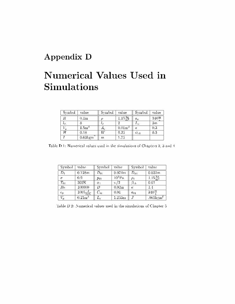
Appendix D
Numerical Values Used in
Simulations
Symbol value Symbol value Symbol value
R 0:1m � 1:15 kgm3 as 340m
s
lE 8 lI 2 Lc 3m
Vp 1:5m3 Ac 0:01m2 a 0:3
H 0:18 W 0:25 c0 0:3
I 0:03kgm2 m 1:75
Table D.1: Numerical values used in the simulations of Chapters 2, 3 and 4.
Symbol value Symbol value Symbol value
D2 0:128m Dt1 0:074m Dh1 0:032m
� 0:9 p01 105Pa �1 1:15 kgm3
T01 303K �1 �=2 �1b 0:61
Re 100000 D 0:02m � 1:4
cp 1005 JkgK
Cm 0:01 a01 340ms
Vp 0:21m3 Lc 1:253m J :001kgm2
Table D.2: Numerical values used in the simulations of Chapter 5.

138 Numerical Values Used in Simulations
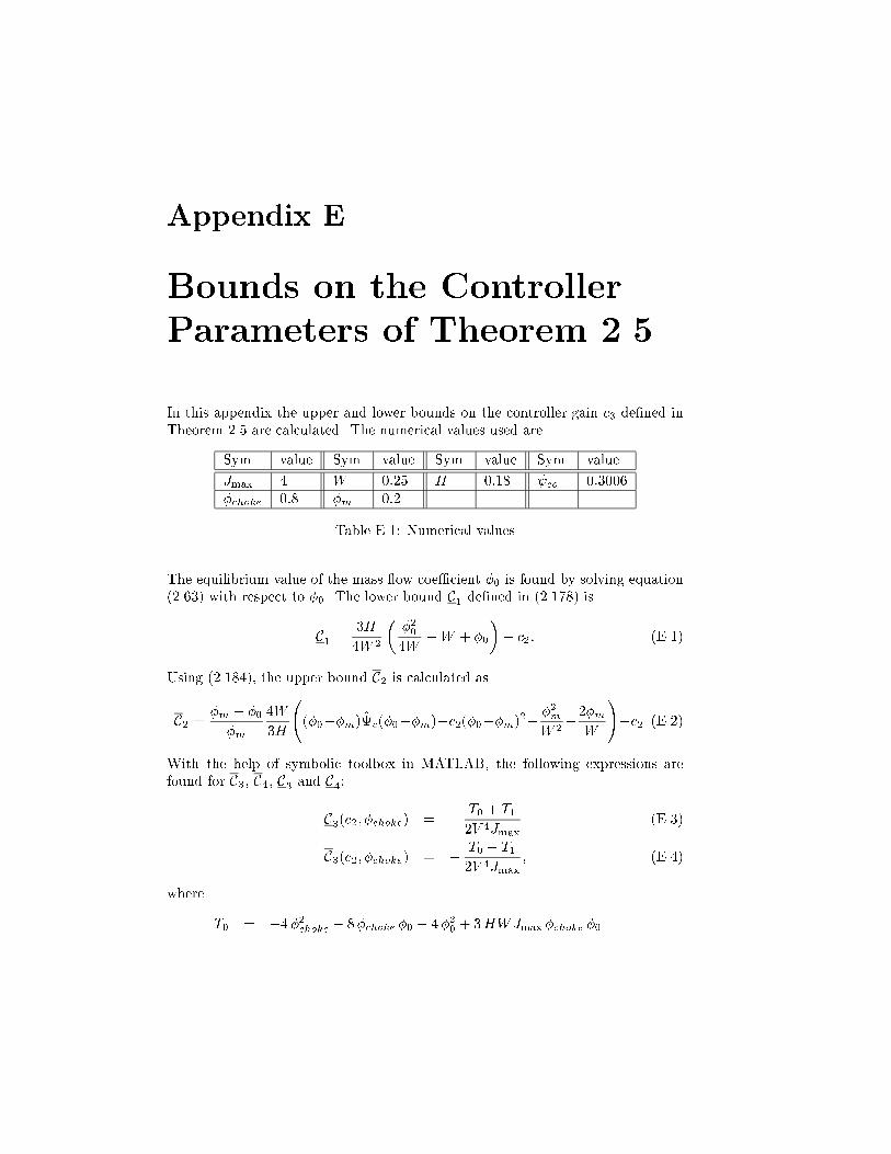
Appendix E
Bounds on the Controller
Parameters of Theorem 2.5
In this appendix the upper and lower bounds on the controller gain c3 de�ned inTheorem 2.5 are calculated. The numerical values used are
Sym. value Sym. value Sym. value Sym. value
Jmax 4 W 0:25 H 0:18 co 0:3006
�choke 0:8 �m 0:2
Table E.1: Numerical values
The equilibrium value of the mass ow coe�cient �0 is found by solving equation(2.63) with respect to �0. The lower bound C1 de�ned in (2.178) is
C1 =3H
4W 2
��204W
+W + �0
�� c2: (E.1)
Using (2.184), the upper bound C2 is calculated as
C2 = �m � �0
�m
4W
3H
(�0��m)c(�0��m)�c2(�0��m)2� �2
m
W 2� 2�m
W
!+c2 (E.2)
With the help of symbolic toolbox in MATLAB, the following expressions arefound for C3, C4, C3 and C4:
C3(c2; �choke) = � T0 + T1
2V 4Jmax(E.3)
C3(c2; �choke) = � T0 � T1
2V 4Jmax; (E.4)
where
T0 = �4�2choke
� 8�choke �0 � 4�20 + 3HWJmax �choke �0
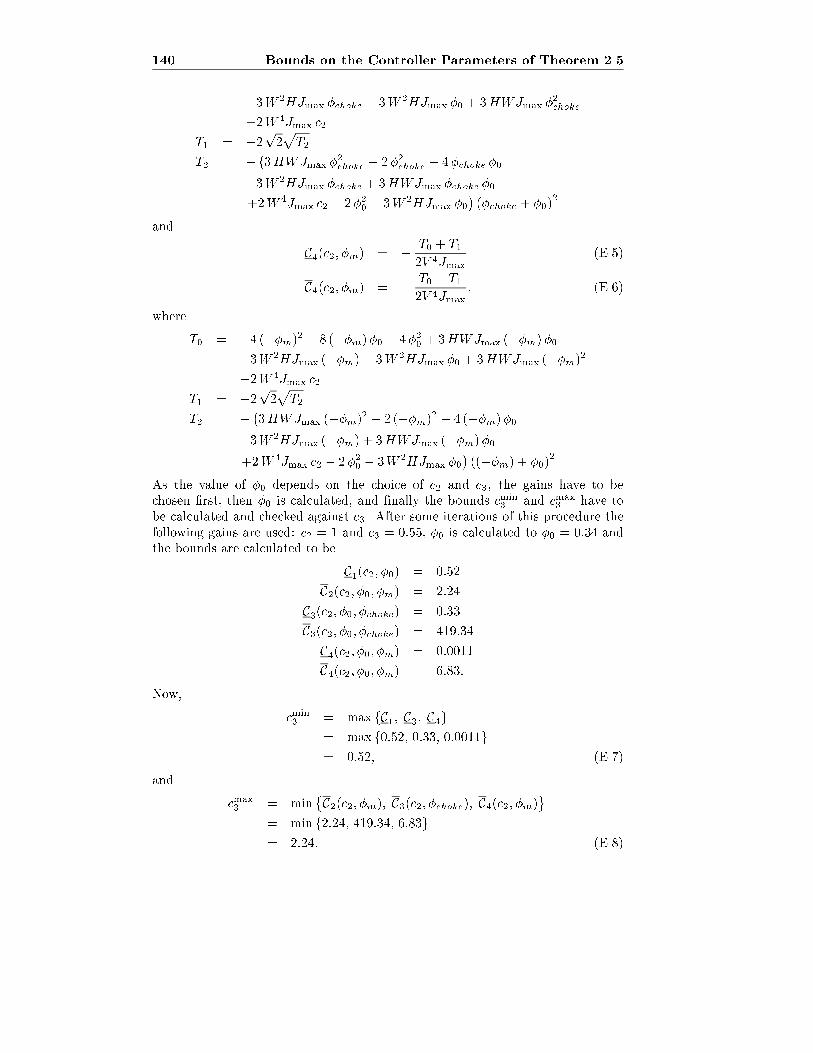
140 Bounds on the Controller Parameters of Theorem 2.5
�3W 2HJmax �choke � 3W 2HJmax �0 + 3HWJmax �2choke
+2W 4Jmax c2
T1 = �2p2pT2
T2 = � �3HWJmax �2choke
� 2�2choke
� 4�choke �0
�3W 2HJmax �choke + 3HWJmax �choke �0
+2W 4Jmax c2 � 2�20 � 3W 2HJmax �0�(�choke + �0)
2
and
C4(c2; �m) = � T0 + T1
2V 4Jmax(E.5)
C4(c2; �m) = � T0 � T1
2V 4Jmax; (E.6)
where
T0 = �4 (��m)2 � 8 (��m)�0 � 4�20 + 3HWJmax (��m)�0�3W 2HJmax (��m)� 3W 2HJmax �0 + 3HWJmax (��m)2+2W 4Jmax c2
T1 = �2p2pT2
T2 = � �3HWJmax (��m)2 � 2 (��m)2 � 4 (��m)�0�3W 2HJmax (��m) + 3HWJmax (��m) �0+2W 4Jmax c2 � 2�20 � 3W 2HJmax �0
�((��m) + �0)
2
As the value of �0 depends on the choice of c2 and c3, the gains have to bechosen �rst, then �0 is calculated, and �nally the bounds cmin3 and cmax3 have tobe calculated and checked against c3. After some iterations of this procedure thefollowing gains are used: c2 = 1 and c3 = 0:55, �0 is calculated to �0 = 0:34 andthe bounds are calculated to be
C1(c2; �0) = 0:52
C2(c2; �0; �m) = 2:24
C3(c2; �0; �choke) = 0:33
C3(c2; �0; �choke) = 419:34
C4(c2; �0; �m) = 0:0011
C4(c2; �0; �m) = 6:83:
Now,
cmin3 = max fC1; C3; C4g= max f0:52; 0:33; 0:0011g= 0:52; (E.7)
and
cmax3 = min�C2(c2; �m); C3(c2; �choke); C4(c2; �m)
= min f2:24; 419:34; 6:83g= 2:24: (E.8)
141
As can be seen the choice c3 = 0:55 now satis�es
cmin3 = 0:52 < c3 = 0:55 < cmax3 = 2:24: (E.9)