arX

iv:h

ep-p

h/96

1244

7v3

19

Mar

199

7

MRI-PHY/96-37

December, 1996

hep-ph/9612447

SOME IMPLICATIONS OF A SUPERSYMMETRIC

MODEL WITH R-PARITY BREAKING BILINEAR

INTERACTIONS

Sourov Roy1 and Biswarup Mukhopadhyaya2

Mehta Research Institute, 10 Kasturba Gandhi Marg, Allahabad - 211 002, INDIA

ABSTRACT

We investigate a supersymmetric scenario where R-parity is explicitly broken through a term

bilinear in the lepton and Higgs superfields in the superpotential. We show that keeping such

a term alone can lead to trilinear interactions, similar to those that are parametrized by λ-

and λ′ in the literature, involving the physical fields. The upper limits of such interactions

are predictable from the constraints on the parameter space imposed by the lepton masses

and the neutrino mass limits. It is observed that thus the resulting trilinear interactions

are restricted to values that are smaller than the existing bounds on most of the λ-and

λ′-parameters. Some phenomenological consequences of such a scenario are discussed.

PACS NOS. : 12.60.Jv, 13.10.+q, 14.80.Ly

1E-mail : sourov@mri.ernet.in

2E-mail : biswarup@mri.ernet.in

1 INTRODUCTION

It is being increasingly realised by those engaged in the search for supersymmetry (SUSY)

[1] that the principle of R-parity conservation, assumed to be sacrosanct in the prevalent

search strategies, is not in practice inviolable. The R-parity of a particle is defined as

R = (−1)L+3B+2S , and can be violated if either baryon (B) or lepton (L) number is not

conserved in nature, a fact perfectly compatible with the non-observation of proton decay.

This is because, whereas the violation of B or L, taken singly, is inadmissible in the standard

model (SM) where all the elementary baryons and leptons are fermions, the SUSY version

of the SM allows it by virtue of the scalar quarks and leptons that are part of the particle

spectrum.

Under R-parity violation the phenomenology changes considerably [2], the most impor-

tant consequence being that the lightest supersymmetric particle (LSP) can decay now.

However, the way in which R-parity can be violated is not unique; different types of R-

violating interaction terms can be written down, leading to different observable predictions.

In addition, R-parity can be violated spontaneously, in stead of explicitly, whence another

class of interesting effects are expected [3]. If the phenomenology of R-parity breaking has

to be understood, and the consequent modifications in the current search strategies have

to be effectively implemented, then it is quite important to explore the full implication of

each possible R-breaking scheme. In this paper we probe some aspects of one such scheme,

namely, where lepton number violation has its origin in terms bilinear in the lepton and

Higgs superfields in the superpotential [4].

The R-conserving part of the minimal supersymmetric standard model (MSSM) is of the

following form in terms of superfields:

WMSSM = ǫab[µHa1H

b2 + hlijL

aiH

b1E

cj + hdijQ

aiH

b1D

cj + huijQ

aiH

b2U

cj ] (1)

1

where (a, b) are SU(2) indices, (i, j) are generation indices and the superscript c denotes right-

handed chiral superfields. Here Q =(

u

d

)

, L =(

νll

)

and H1, H2 are the Higgs superfields that

gives masses to the down- and up-type quark superfields. If now R-breaking interactions are

incorporated, the superpotential takes the form [5]

W =WMSSM +WL +WB (2)

with

WL = ǫab[λijkLaiL

bjE

ck + λ′ijkL

aiQ

bjD

ck + ǫiL

aiH

b2] (3)

and

WB = λ′′ijkUciD

cjD

ck (4)

Obviously, both WL and WB cannot be present if the proton has to be stable. In the rest

of this paper we shall concentrate on the case where only lepton number is violated.

WB as well as the first two terms in WL have received a lot of attention in recent times,

and constraints have been derived on them from existing experimental data [6]. However,

the term ǫiLaiH

b2 is also a viable agent for R-parity breaking. It is particularly interesting

for the fact that it can trigger a mixing between charginos and charged leptons as well as

between neutralinos and neutrinos, resulting in observable effects that are not to be seen with

the λ-and λ′-terms alone. One of these distinctive effects is that, the lightest neutralino can

decay invisibly into three neutrinos, which is not possible if only the first two terms in WL

are present. Some other implications, especially those in the scalar sector of the theory, have

been investigated recently in the literature [7]. The significance of such bilinear R-violating

interactions is further emphasized by the following observations:

2

(1) Although it may seem possible to rotate away the LH2-terms by redefining the lepton

and Higgs superfields, their effect is bound to show up via the scalar potential [7].

(2) Even if one may rotate away these terms at one enrgy scale, they reappear at another as

the couplings evolve radiatively [8].

(3) the λ-and λ′-terms themselves give rise to the bilinear terms at the one-loop level [9].

(4) It has been argued that if one wants to subsume R-parity violation in a Grand Unified

Theory (GUT), then the trilinear interactions in WL naturally come out to be rather small

in magnitude (O(10−3) or so) [10]. However, the superrenormalizable bilinear terms are not

subjected to such requirements a priori.

We perform an analysis here keeping ǫLH2 as the only R-parity violating term in the

theory [11]. Moreover, for reasons that we shall discuss below, we are incorporating such

a term only for the third generation lepton superfield L3. We shall see that after one

incorporates the effect of mixing, such a term can give rise to trilinear interactions among

the physical states, which are very similar in nature to those induced by the λ’s and the

λ′’s. All these interactions are derived in section 2, together with the gauge boson couplings

of the lepton-chargino and neutrino-neutralino physical states. It is interesting to note that

the parameters giving rise to these interactions are constrained by the τ -and ντ masses.

Thus it is possible to predict the maximum possible values for the couplings for any given

set of parameters of the MSSM. In section 3 we discuss these constraints and some of their

phenomenological consequences. Our conclusions are summarised in section 4. The detailed

forms of some formulas of section 2 are presented in the appendix.

3

2 The Formalism

As has been stated before, we consider a superpotential of the form

W =WMSSM + ǫL3H2 (5)

where the SU(2) indices have been suppressed. The simplification achieved by letting only the

third generation mix with the Higgs superfield can be justified if one notes that the value of

ǫi for a particular generation is constrained severely by the upper limit on the neutrino mass

in that generation. Since the τ -neutrino mass has the least restrictive laboratory bound of

24 MeV [12], only ǫ3 (to be called ǫ hereafter) can be large enough to be phenomenologically

significant.

An immediate consequence of a non-zero ǫ is the mixing between the charged leptons

and the charginos as well as between neutrinos and neutralinos. The other quantity that

can trigger such mixing is a non-zero vacuum expectation value (vev) of ντ . This vev leads

to off-diagonal ντ − Z and τ − W terms in the current eigenstate basis [13].

In such a situation, the (3×3) chargino mass matrix is

Mχ± =

M −gv2 0

−gv1 µ fv3

−gv3 ǫ −fv1

(6)

where v1 = 〈H1〉, v2 = 〈H2〉, v3 = 〈ντ 〉 and f = hl33 = mτ

v1, M being the SU(2)

gaugino mass parameter. Here we have assigned (−i ¯W−, ¯H−1 , τL

−) along the rows and

(−i ¯W+, ¯H+2 , τR

+) along the columns. Similarly, the extended neutralino mass matrix in

4

the basis (−iA,−iZ, H01 , H

02 , ντ ) is given by

Mχ0 =

MA12(MZ −MA)tan2θW 0 0 0

12(MZ −MA)tan2θW MZ − gv1√

2cosθW

gv2√2cosθW

− gv3√2cosθW

0 − gv1√2cosθW

0 −µ 0

0 gv2√2cosθW

−µ 0 −ǫ

0 − gv3√2cosθW

0 −ǫ 0

(7)

with

MA =M ′cos2θW +Msin2θW (8)

MZ =M ′sin2θW +Mcos2θW (9)

M ′ and M being respectively the U(1) and SU(2) gaugino mass parameters.

The diagonalisation of Mχ± and Mχ0 is straightforward; one thus obtains two (3×3)

matrices U and V for the right-handed and left-handed chargino respectively and a (5×5)

mixing matrix N for the neutralinos. These correspond to their MSSM forms in the proper

limit.

Let us now consider the scalar sector in this scenario. The scalar potential, including the

third generation sleptons, is given by

V = m21H

†1H1 +m2

2H†2H2 +m2

Lτ †LτL +m2

Rτ †RτR +m2

ντν†τ ντ

+f 2H†1H1(L

†L+ τ †RτR) + f 2L†Lτ †RτR + µf [H†2Lτ

†R + L†H2τR]

−ǫf [H†1 τRH2 +H1τ

†RH

†2] + µǫ[LH†

1 + L†H1]− f 2H†1L(H

†1L)

†

+B1µ(φ01φ

02 − φ−

1 φ+2 + φ0

2†φ01† − φ+

2†φ−1†) + Af(τLφ

01 − ντφ−

1 )τ†R

+B2ǫ(ντφ02 − τLφ+

2 + φ02†ν†τ − φ+

2†τ †L) + Af(τ †Lφ

01† − ν†τφ−

1†)τR

+1

8(g2 + g′

2)[(H†

1H1 −H†2H2)

2] +

1

2g2|H†

1H2|2

−12g′

2τ †RτR(L

†L+H†1H1 −H†

2H2)

5

+1

4g2(ν†τ τLτ

†Lντ ) +

1

2g2(ν†τ τLφ

−1†φ01 + τ †Lντφ

01†φ−1 )

+1

4g2(ν†τ ντφ

01†φ01 + τ †LτLφ

−1†φ−1 − ν†τ ντφ−

1†φ−1 − τ †LτLφ0

1†φ01)

+1

4g2(ν†τ ντφ

+2†φ+2 + τ †LτLφ

02†φ02 − ν†τ ντφ0

2†φ02 − τ †LτLφ+

2†φ+2 )

+1

2g2(ν†τ τLφ

02†φ+2 + τ †Lντφ

+2†φ02) +

1

4g′

2τ †LτL(H

†1H1 −H†

2H2) +1

4g′

2(ν†τ τLτ

†Lντ )

+1

8(g′

2+ g2)(ν†τ ντ )

2+ (τ †LτL)

2 (10)

where L =(

νττ

)

L, H1 =

(

φ01

φ−

1

)

, H2 =(

φ+

2

φ02

)

. A is the SUSY breaking trilinear soft term and

B1, B2 are the bilinear soft terms.

The mass-squared matrices for the neutral scalars, neutral psedoscalars and charged

scalars are given respectively by

M2s =

m21 + 2λc+ 4λv21 −4λv1v2 +B1µ 4λv1v3 + µǫ

−4λv1v2 +B1µ m22 − 2λc+ 4λv22 −4λv3v2 +B2ǫ

4λv1v3 + µǫ −4λv3v2 +B2ǫ m2ντ

+ 2λc+ 4λv23

(11)

M2p =

m21 + 2λc −B1µ µǫ

−B1µ m22 − 2λc −B2ǫ

µǫ −B2ǫ m2ντ

+ 2λc

(12)

and

Mc2 =

r − 14g′2c −B1µ+ 1

2g2v1v2 −B2ǫ+

12g2v2v3 −ǫfv1

−B1µ+ 12g2v1v2 s+ 1

4g′2c µǫ+ 1

2g2v1v3 −ǫfv2 + Afv3

−B2ǫ+12g2v2v3 µǫ+ 1

2g2v1v3 p + 1

4g2t + 1

4g′2c µfv2 − Afv1

−ǫfv1 −ǫfv2 + Afv3 µfv2 − Afv1 q − 12g′2c + f 2v3

2

(13)

with

r = m22 +

1

4g2(v21 + v22 + v23)

s = m21 +

1

4g2(v21 + v22 − v23)

6

p = m2L+ f 2v21

q = m2R+ f 2v21

t = (−v21 + v22 + v23)

c = (v21 − v22 + v23)

λ = (g2 + g′2)/8

Here the real and imaginary part of ντ enter intoMs2 andMp

2 respectively. The correspond-

ing diagonalising matrices that control the mixing in those sectors are described here as S,

P and C.

The scalar sector is subject to the following constraints [14] :

(1) The extremization of the neutral part of the potential leads to

(m21 + 2λc)v1 +B1µv2 + µǫv3 = 0 (14)

(m22 − 2λc)v2 +B1µv1 +B2ǫv3 = 0 (15)

(m2ντ

+ 2λc)v1 +B1µv2 + µǫv3 = 0 (16)

Furthermore, the second derivatives with respect to the neutral fields at the extremum must

be all positive.

(2) The potential must be bounded from below [15]. The resulting condition is

m21(v

22 − v23) +m2

2v22 +m2

ντv23 + 2µǫ(v22 − v23)

1

2v3

+2B1µ(v22 − v23)

1

2 v2 + 2B2ǫv2v3 ≥ 0 (17)

Note that setting v3 = 0 above give us the corresponding condition in MSSM.

7

(3) Gauge symmetry breaking requires that the minimum of the potential has to be negative

[16]. This implies

Xmin ≤ 0 (18)

where Xmin is the lowest eigenvalue of the matrix

m21 B1µ µǫ

B1µ m22 B2ǫ

µǫ B2ǫ m2ντ

(19)

(4) All the eigenvalues of the M2s ,M

2p and M2

c have to be non-negative. This leads to the

necessary (but not sufficient) conditions that B1 and µ, as also B2 and ǫ, are of opposite

signs.

Once the five mass matrices mentioned above are diagonalised, we are in a position to

write down all the interactions in terms of the physical fields in the spin-12and spin-0 sectors.

We emphasize that it is the couplings of these physical fields that are going to be ultimately

related to experimental observables. Hence any phenomenological constraint that is relevant

should basically apply to them.

Now, the physical scalar states that are dominantly charged sleptons or sneutrinos have

Higgs components in them. Similarly, there are bound to be some gaugino (or Higgsino)

admixtures in the states which are mostly τ or ντ . Consequently, the Higgs and gaugino

interactions of leptons (in the current eigenstate basis) give rise to trilinear interaction terms

involving dominantly leptonic (or sleptonic) fields. Similar interactions of the quarks can

also give rise to L-violating interactions. Thus we notice that starting from the bilinear

interaction LH2, trilinear couplings of physical states very similar to those conventionally

parametrized by λ and λ′ automatically emerge.

In the interactions presented below, we have designated by ei, νi(ei, νi) the fermion

(scalar) mass eigenstates which are dominantly leptons (sleptons) of the i th generation.

8

The scalar (pseudoscalar) dominated by the real (imaginary) part of νiL is described as

νiL1(νiL2). Thus we end up with trilinear terms in the Lagrangian,given by

Ltr = L1 + L2 (20)

with

L1 = ρi3ie∗iL e

3cR νL

i + ρ′333e3Le

3RνL

3 + ωi3iνiL1e

3ReL

i

+ω′i3iν

iL2e

3ReL

i + ηi3ie∗iL ν

3cL eL

i + ξi3iν∗iL ν

3cL νL

i

+ζii3eiRe

iRνL

3 + ζ ′333e∗3R e

3cR νL

3 + δ333e∗3R ν

3cL eL

3 +H.c., (21)

L2 = Ω3iie3cR uL

id∗iL + Ω′3iie

3RdL

iu∗iL + Λi3iuiLνL

3cuiL

+Λ′i3id

iLνL

3cdiL + Λ′′i3iu

iRνL

3uiR + Λ′′′i3id

iRνL

3diR

+Ψij3diRuL

j e3L +Ψ′ij3d

iRuL

j e3R +Ψ′′3ij e

3cR uL

id∗jR

+Ψ′′′3ij ν

3cL dL

id∗jR +∆i3j diReL

3ujL +∆′i3j d

iRνL

3djL

+∆′′ij3d

iRdL

j ν3L1 +∆′′′ij3d

iRdL

j ν3L2 + Σ3ij e3RdL

iu∗jR

+Σ′3ij ν

3cL uL

iu∗jR + Σ′′ij3u

iRdL

j e∗3L + Σ′′′ij3u

iRdL

j e∗3R

+χij3uiRuL

j ν3L1 + χ′ij3u

iRuL

j ν3L2 + χ′′i3j u

iReL

3cdjL

+χ′′′i3j u

iRνL

3ujL +H.c. (22)

where the notation used for the quark and squark fields is obvious. The detailed expressions

for the different couplings in terms of the elements of the mixing matrices will be found in

the Appendix. Wherever the index 3 has been kept fixed in the couplings, it is because only

the third generation of leptons mixes with Higgs in this picture.

It is instructive to compare the above Lagrangian with that obtained from λ- and λ′-type

trilinear terms in the superpotential. In the notation of reference [5], such interactions are

Lλ = λijk[νiLe

kReL

j + ejLekRνL

i + ek∗R νciL eL

j − (i←→j)] + H.c., (23)

9

Lλ′ = λ′ijk[νiLd

kRdL

j + djLdkRνL

i + dk∗R νciL dL

j − eiLdkRuLj − ujLdkReLi − dk∗R eciLuLj ] + H.c. (24)

First of all, all the terms in equation (23) can be generated in L1 if one allows for mixing of

the three leptonic generations and also Yukawa coupling of the first two generations. The fact

that we have neglected both of the above features is responsible for the absence of coefficients

in equation (21) with all three indices different. On the other hand, L1 can contain coefficients

with generation indices iii (in our case, 333 only because of reasons stated above). Such

terms are forbidden in equation (23) by gauge invariance of the superpotential, unless there

is mixing among the lepton generations.

Next, we note that the terms in L1 proportional to ρ, η, ξ, ζ and ζ ′ do not arise in (23).

The ρ-term owes its structure to the gaugino and Higgsino couplings in the MSSM part of

the Lagrangian. The four remaining terms also could not be allowed in (23) because, again,

SU(2) invariance of the superpotential would forbid terms with either three left chiral fields

or one left and two right chiral fields. A particularly interesting consequence of this is the

presence of trilinear interaction involving a sneutrino and two neutrino physical fields. This

lends considerable additional phenomenology to the scenario under study here. For example,

a sneutrino can decay into two neutrinos here [7]. Also, as we shall see below, it entails the

possibility of invisible decays of the lightest neutralino.

On comparing equations (22) and (24) we find that all the λ′-type terms are generated

in L2 as well. In addition, there are several more terms which are prevented in (24) in order

to prevent weak isospin and hypercharge violation in the superpotential.

The other novel consequences of the LH2 term are the flavor-changing couplings of theW

and the Z. Although it has been sometimes claimed in the literature [17] to be a signature

of spontaneous R-parity violation, in practice it follows just from the bilinear terms of the

type discussed by us. Diagonalisation of the mass matricesMχ± andMχ0 immediately imply

10

that now there can be a tree-level interaction involving a τ(ντ ) dominated physical state,

a neutralino (chargino)-dominated state and a W . Similarly, the fact that the neutralinos

(charginos) and the ντ (τ) differ in T3 and Y implies that their Z-couplings can now be

non-diagonal. The interactions are given by

LW−χ+χ0 = gWµ− ¯χ0

iγµ[ OL

ijPL +ORijPR ]χ+

j +H.c., (25)

L¯χχZ =g

cosθW[ ¯χiγ

µ(O′LijPL +O′R

ijPR)χj ]Zµ +H.c., (26)

L¯χ0χ0Z

=g

cosθW[1

2¯χ0iγ

µ(O′′LijPL +O′′R

ijPR)χ0j ]Zµ +H.c. (27)

where the detailed forms of the matrices O, O′ and O′′ are relegated to the Appendix.

We end this section by re-iterating that the bilinear interaction LH2 is sufficient to

generate all the λ- and λ′-type terms involving physical fields. They also give rise to other

trilinear interaction terms which are otherwise disallowed. Furthermore, the postulate that

only the third generation is involved in L-violating mixing (partially justified by the observed

mass hierarchy) suggests that flavor changing trilinear terms should be smaller in magnitude.

3 Numerical Results

In order to find out the allowed region in the parameter space, one has to take a number of

constraints into account. First, we note that ǫ and v3 are the only parameters outside MSSM

that enter into the chargino and neutralino mass matrices. The strongest constraint on them

follows from the fact that the τ -mass has been experimentally measured [12]. Therefore, for

any combination of the MSSM parameters (mg, µ, tanβ), the lowest eigenvalue ofmχ± should

agree with mτ for any combination of ǫ and v3. Also, ντ has a laboratory upper limit of 24

11

MeV on its mass. These two restrictions, taken together, constrain the ǫ − v3 space in a

severe manner.

Figures (1 − 4) show the allowed areas of the ǫ − v3 parameter space for several combi-

nations of the MSSM parameters. Here, in addition to the constraint mντ < 24 MeV the

lowest eigenvalue of the mχ± has been allowed at most a 3σ-deviation from the measured

central value of mτ . However, there is an extra parameter here to play with, namely, the

third diagonal entry of mχ± . In the figures presented here, we have fixed this term at the

central experimental value of mτ , viz. 1.777 GeV. The allowed area slightly increases on

varying this mass parameter, but it is not permissible to drift too much from the value used

here. It is easy to check that our allowed region is consistent at 95 % confidence level with

the restrictions imposed by the global fit of LEP data and low energy experiments on the

mixing of the τ and the ντ with exotic fermions [18]. In any case, we find that there is

no substantial allowed region with |ǫ| and v3 larger than about 20 and 5 GeV respectively.

Sometimes there are extremely narrow allowed bands with one of them of a considerably

higher value. Such “fine-tuned” areas are not used in our subsequent calculations.

The next set of constraints arise from the scalar sector where all of the four conditions

mentioned in the previous section have to be fulfilled. The scalar potential introduces several

new parameters: m1, m2, m0 (the slepton/sneutrino mass assuming a degeneracy), A,B1 and

B2. Of these, the minimisation conditions imply that only three are independent. We have

chosen A, B1 and B2 to be the three independent parameters. Furthermore, we set A equal

to zero to simplify our analysis. Now, taking ǫ and v3 from the allowed regions described

above, one gets restricted in the choice of B1 and B2. A definite requirement in this respect

is that B1(B2) should have a sign opposite to that of µ(ǫ).

Having thus been guided to the allowed region in the entire parameter space, we can

now compute all the R-parity violating couplings in terms of them. We have neglected all

12

CP-violating phases. The values of these for some sample values of the SUSY parameters

are shown in Tables 1 and 2. The numbers indicate the maximum values that the respective

couplings can have. Most of the couplings are seen to be on the order of 10−3 or less,

excepting a few on the order of 10−2 or even 10−1. It is noticeable that a higher value of ǫ

often raises the couplings. The cases where this does not happen can be ascribed to enhanced

cancellations among the different terms that comprise a particular coupling. In particular,

an enhancement in some of the terms occurs when the slepton mass m0 is close to one of the

Higgs masses, which causes a large slepton(sneutrino)- Higgs mixing. Wherever such mixing

terms dominate in any interaction strength, the corresponding strength is large.

In general, the R-violating interactions that we obtain here after satisfying all requisite

constraints are considerably smaller than the bounds on the analogous λ- and λ′-type terms

derived in the literature from existing experimental data. The latter includes limits from

a wide variety of phenomena, from low-energy weak processes to results from the Large

Electron Positron (LEP) collider. This suggests that if indeed bilinear interactions are the

real sources of the nonconservation of R-parity, then our experimental precision requires

considerable improvement before such interactions can be probed.

Finally, let us turn to some processes that can be looked upon as the typical consequences

of bilinear R-violating terms. Of course, the lightest neutralino χ0 (the LSP in MSSM) is

bound to be unstable. When its mass is less than that of the standard gauge bosons, it can

only have three-body decays. The final states for such decays are the same whether R-parity

is violated originally through bilinear or trilinear interactions.

However, if mχ0 is larger than mZ , mW , then the bilinear terms in our scenario open up

two-body decay channels which are not otherwise possible. These are the channels χ0 −→

τW and χ0 −→ ντZ, controlled by OL(R), O′L(R) and O

′′L(R) of equations 25-27. In Table 3

we list their values for the same set of input parameters as in Tables 1 and 2.

13

Figures 5 and 6 contain some plots for the dominant branching ratios, assuming that

χ0 −→ τW and χ0 −→ ντZ are the only available channels. The former mode is found

to dominate in figure 5, while the latter takes over in figure 6. This is because there are

essentially two main components in each of the χ0τW and χ0ντZ interactions. One of

these comes from the neutrino-tau(neutrino)-W(Z) gauge couplings, and the other, from

the Higgsino-Higgsino-W(Z) coupling. In the area of the parameter space shown in figure

5, it is found that while the two components add up in the former process, they interfere

destructively in the latter, causing a large cancellation. Exactly the opposite thing happens

in figure 6, where, in particular, |µ|, |B1| and |B2| are large. This indicates that pair-produced

neutralinos are expected to give rise to signals of the form ττWW and ZZ + 6 pT . R-parity

violation through bilinear interaction terms is quite characteristically reflected through such

signals.

4 Summary and Conclusions

We have studied the effects of an R-parity violating bilinear term L3H2 in the superpotential.

We find that this term, together with a sneutrino vev, leads to trilinear couplings involv-

ing dominantly leptonic and sleptonic (as also two quarks/squarks and one lepton/slepton)

physical fields. We emphasize that it is these terms involving physical fields which are of phe-

nomenological significance. The interactions thus generated include the λ- and λ′-type ones

which follow from trilinear R-parity violating terms in the superpotential. In addition, we

obtain several terms that are not permitted in the other case. The most noteworthy among

them is the one involving a sneutrino and two neutrinos. Also, there arise off-diagonal inter-

actions of charginos and neutralinos with τ and ντ coupled to a W or a Z. Such interactions

are the characteristic features of bilinear R-violation. The parameter space of such a scenario

14

can be best limited by restricting the lowest eigenvalues of the chargino and neutralino mass

matrices. Further constraints follow from requirements of electroweak symmetry breaking in

the scalar sector. The trilinear couplings thus generated mostly turn out to be small com-

pared to their current phenomenological limits. Thus if bilinear terms are the sole sources

of R-parity violation, then the restrictions imposed by the lepton and neutrino masses are

still more stringent than any other experimental bound. And finally, we have discussed some

phenomenological consequences of such a scenario. In particular, we show that if the lightest

neutralino is heavier than the weak gauge bosons, then its dominant decay occurs in the

channels χ0 −→ τW and χ0 −→ ντZ giving rise to rather characteristic signals.

Acknowledgement

We thank P. K. Mohanty, A. Rastogi, Suresh Rao and A. Ghosal for computational help and

A. Kundu and A. Datta for helpful discussions.

15

Appendix A

Here we present the full forms of the various couplings in equations (21) and (22). In ob-

taining the trilinear interactions, the mixing among leptons and quarks in gaugino couplings

have been neglected. Using the notation already established in the text,

ρ131 = ρ232 = −gU∗31 (A.1)

ρ333 = −gU∗31 + fU∗

32N∗55C43 (A.2)

ρ′333 = fV ∗33N

∗55C23 − fV ∗

33N∗53C33 (A.3)

ω131 = ω232 = −gV ∗31 (A.4)

ω333 = −gV ∗31 +

1√2fV ∗

33U∗32S33 −

1√2fV ∗

33U∗33S13 (A.5)

ω′131 = ω′

232 = gV ∗31 (A.6)

ω′333 = gV ∗

31 +1√2fV ∗

33U∗32P33 −

1√2fV ∗

33U∗33P13 (A.7)

η131 =√2 eN∗

51 −√2 g

cosθW(−1

2+ sin2θW )N∗

52 (A.8)

η232 =√2 eN∗

51 −√2 g

cosθW(−1

2+ sin2θW )N∗

52 (A.9)

η333 =√2 eN∗

51 −√2 g

cosθW(−1

2+ sin2θW )N∗

52 − fN∗53U

∗33C43 (A.10)

ξ131 = −√2 g

2cosθWN∗

52 (A.11)

16

ξ232 = −√2 g

2cosθWN∗

52 (A.12)

ξ333 = −√2 g

2cosθWN∗

52 (A.13)

ζ113 = −√2 eN∗

51 +

√2 gsin2θWcosθW

N∗52 (A.14)

ζ223 = −√2 eN∗

51 +

√2 gsin2θWcosθW

N∗52 (A.15)

ζ333 = −√2 eN∗

51 +

√2 gsin2θWcosθW

N∗52 + fV ∗

33N∗55C24 − fV ∗

33N∗53C34 (A.16)

ζ ′333 = fU∗32N

∗55C44 (A.17)

δ333 = −fU∗33N

∗53C44 (A.18)

Ω3ii = −gU∗31 (A.19)

Ω′3ii = −gV ∗

31 (A.20)

Λi3i = −√2 g

cosθW(1

2− 2

3sin2θW )N52 +

2

3g sinθWN51 (A.21)

Λ′i3i =

√2 g

cosθW(−1

2+

1

3sin2θW )N52 −

1

3g sinθWN51 (A.22)

Λ′′i3i = −

√22

3

g

cosθWsin2θWN

∗52 −

2

3g sinθWN

∗51 (A.23)

Λ′′′i3i =

√2−1

3

g

cosθWsin2θWN

∗52 +

1

3g sinθWN

∗51 (A.24)

17

Ψij3 = f1C23 (A.25)

Ψ′ij3 = f1C24 (A.26)

Ψ′′3ij = f1U

∗32 (A.27)

Ψ′′′3ij = −f1N∗

53 (A.28)

∆i3j = f1U∗32 (A.29)

∆′i3j = −f1N∗

53 (A.30)

∆′′ij3 = −

1√2f1S13 (A.31)

∆′′′ij3 = −

1√2f1P13 (A.32)

Σ3ij = f2V∗32 (A.33)

Σ′3ij = −f2N∗

54 (A.34)

Σ′′ij3 = f2C13 (A.35)

Σ′′′ij3 = f2C14 (A.36)

χij3 = −1√2f2S23 (A.37)

χ′ij3 = −

1√2f2P23 (A.38)

18

χ′′i3j = f2V

∗23 (A.39)

χ′′′i3j = −f2N∗

54 (A.40)

f1 and f2 are defined above as f1 = hd33 =mb

v1, f2 = hu33 =

mt

v2. We have neglected the Yukawa

interactions of the remaining quarks.

Next we give detailed forms of the matrices O, O′ and O′′ which appear in equations (25)-

(27).

OLij =

1√2Ni4V

∗j2 − cosθWNi2V

∗j1 − sinθWNi1V

∗j1 (A.41)

ORij = −

1√2N∗

i3Uj2 − cosθWN∗i2Uj1 − sinθWN

∗i1Uj1 +

1√2N∗

i5Uj3 (A.42)

O′ijL= Vi1V

∗j1 +

1

2Vi2V

∗j2 − δijsin2θW + Vi3V

∗j3sin

2θW (A.43)

O′ijR= U∗

i1Uj1 +1

2U∗

i2Uj2 − δijsin2θW + U∗i3Uj3(−

1

2+ sin2θW ) (A.44)

O′′ijL=

1

2Ni3N

∗j3 −

1

2Ni4N

∗j4 +

1

2Ni5N

∗j5 (A.45)

O′′ijR= −1

2N∗

i3Nj3 +1

2N∗

i4Nj4 = −O′′ijL

(A.46)

19

References

[1] For reviews see, for example, H.P. Nilles, Physics Reports 110, 1(1984); H.E. Haber

and G.L. Cane, Physics Reports 117, 75(1985).

[2] See, for example, R. Barbieri and L. Hall, Phys. Lett. B238, 86(1990); V. Barger et

al., Phys. Rev. D44, 1629(1991); R. Godbole, P. Roy and X. Tata, Nucl. Phys. B401,

67(1993)

[3] C.S. Aulakh and R.N. Mohapatra, Phys. Lett. 119, 136(1982); A. Masiero and T.

Valle, Phys. Lett. B251, 273(1990); G. Giudice et al., Nucl. Phys. B396, 243(1993); I.

Umemura and K.Yamamoto, Nucl. Phys. B423, 405(1994).

[4] S. Dawson, Nucl. Phys. B261, 297(1985).

[5] V. Barger, G. Giudice and T. Han, Phys. Rev. D40, 2987(1989).

[6] G. Bhattacharyya, D. Choudhury and K. Sridhar, Phys. Lett. B349, 118(1995); G.

Bhattacharyya, D. Choudhury and K. Sridhar, Phys. Lett. B355, 193(1995); G. Bhat-

tacharyya, J. Ellis and K. Sridhar, Mod. Phys. Lett. A10, 1583(1995); Alexei Yu.

Smirnov and Francesco Vissani, Phys. Lett. B380, 317(1996); K. Agashe and M.

Graesser, Phys. Rev. D54, 4445(1996).

[7] F. de Campos et al., Nucl. Phys. B451, 3(1995).

[8] V. Barger et al., Phys. Rev. D53, 6407(1995).

[9] B. de Carlos and P. L. White, Phys. Rev. D54, 3427(1996).

[10] L. Hall and M. Suzuki, Nucl. Phys. B231, 419(1984).

20

[11] For other recent works on this topic, see, for example, A. Joshipura and M. Nowakowski,

Phys. Rev. D51, 2421(1995); ibid, 5271(1995); M. Nowakowski and A. Pilaftsis, Nucl.

Phys. B461, 19(1996); R. Hempfling, Nucl. Phys. B478, 3(1996); T. Banks et al., Phys.

Rev. D52, 5319(1996); H. P. Nilles and N. Polonsky, Nucl. Phys. B484, 33(1997).

[12] Review of Particle Properties, Particle Data Group, Phys. Rev. D54, (1996).

[13] G. Ross and J. Valle, Phys. Lett. B151, 375(1985).

[14] For the discussion for MSSM, see, for example, I. Simonsen, hep-ph/9506369.

[15] A. Bouquet et al., Nucl. Phys. B262, 299(1985).

[16] For the corresponding MSSM case, see J. Gunion and H. Haber, Nucl. Phys. B278,

449(1986).

[17] M. Gonzalez-Garcia et al., Nucl. Phys. B391, 100(1993); J. Romao et al., hep-

ph/9604244.

[18] E. Nardi et al., Phys. Lett. B344, 225(1995).

21

Table 1

ǫ = 16 ǫ = 2

ρ131 0.00633 -0.00589

ρ232 0.00633 -0.00589

ρ333 0.00776 -0.00597

ρ′333 -8.1 × 10−6 -0.00014

ω131 -0.00018 0.00017

ω232 -0.00018 0.00017

ω333 -0.00027 -0.00036

ω′131 0.00018 -0.00017

ω′232 0.00018 -0.00017

ω′333 0.00020 -0.00031

ǫ = 16 ǫ = 2

η131 -0.00137 0.00128

η232 -0.00137 0.00128

η333 -0.00279 0.00137

ξ131 0.00422 -0.00393

ξ232 0.00422 -0.00393

ξ333 0.00422 -0.00393

ζ113 -0.00413 0.00384

ζ223 -0.00413 0.00384

ζ333 -0.00413 0.00399

ζ ′333 0.00128 -0.00009

δ333 -0.00127 0.00010

Table 1:

Sample values of the couplings in equation 21, for two values of ǫ, with v3 = 3.4, µ = 200,

mg = 750, B1 = -180, B2 = -160, tanβ = 2. All the mass parameters are expressed in GeV.

22

Table 2

ǫ = 16 ǫ = 2

Ω3ii 0.00633 -0.00589

Ω′3ii -0.00018 0.00017

Λi3i 0.00275 -0.00256

Λ′i3i 0.00584 -0.00543

Λ′′i3i 0.00235 -0.00219

Λ′′′i3i 0.00117 -0.00109

ψij3 0.00308 -0.00059

ψ′ij3 -0.00344 0.00057

ψ′′3ij -0.00467 -0.00029

ψ′′′3ij 0.00464 0.00033

∆i3j -0.00467 -0.00029

ǫ = 16 ǫ = 2

∆′i3j 0.00464 0.00033

∆′′ij3 0.00309 -0.00151

∆′′′ij3 0.00335 -0.00054

Σ3ij 0.00048 -0.00045

Σ′3ij -0.00238 0.00223

Σ′′ij3 0.01521 0.01113

Σ′′′ij3 -0.01649 -0.01182

χij3 -0.01785 -0.04348

χ′ij3 0.01674 0.01170

χ′′i3j 0.00048 -0.00045

χ′′′i3j -0.00238 0.00223

Table 2:

Sample values of the couplings in equation 22, with the same input parameters as in Table

1.

23

Table 3

ǫ = 16 ǫ = 2

OL51 0.00412 -0.00385

OR51 0.06329 -0.01545

OL52 -0.00640 0.00595

OR52 0.10156 0.00201

OL43 0.00016 -0.00015

OR43 -0.05506 0.00550

O′L32 -0.00023 0.00022

O′R32 -0.05813 -0.00390

O′L31 0.00006 -0.00006

O′R31 -0.03097 0.01152

O′′L45 -0.00501 0.00467

O′′R45 -0.01581 -0.00146

Table 3:

Sample values of the couplings in equations 25-27, with the same input parameters as in

Table 1.

24

Figure Captions

Figure 1:

The allowed region(dark) in the ǫ-v3 parameter space, with B1 = -180, B2 = -160, µ = 200,

tanβ = 2, mg = 750. All mass parameters are expressed in GeV.

Figure 2:

Same as in Figure 1, with B1 = -160, B2 = -170, µ = 200, tanβ = 10, mg = 750.

Figure 3:

Same as in Figure 1, with B1 = 150, B2 = 170, µ = -200, tanβ = 2, mg = 300.

Figure 4:

Same as in Figure 1, with B1 = 150, B2 = 200, µ = -200, tanβ = 2, mg = 750.

Figure 5:

B(χ0 −→ τW ) plotted against the lightest neutralino mass (in GeV). The bold (thin) line

corresponds to tanβ = 2, B1 = -180, B2 = -160, ǫ = 5.0, v3 = 2.0 µ = 200 (tanβ = 10, B1

= -160, B2 = -170, ǫ = 1.0, v3 = 0.4, µ = 200). All mass parameters are expressed in GeV.

Figure 6:

B(χ0 −→ ντZ) plotted against the lightest neutralino mass (in GeV). The bold (thin) line

corresponds to tanβ = 2, B1 = -350, B2 = -330, ǫ = 10.0, v3 = 3.0 µ = 500 (tanβ = 10, B1

= -280, B2 = -290, ǫ = 4.0, v3 = 1.0, µ = 500).

25

0 5 10 15 20 25 30

0

1

2

3

4

5

6

7

Figure 1

ε

v3

0 5 10 15 20 25 30

0

1

2

3

4

5

6

7

Figure 2

ε

v3

-30 -25 -20 -15 -10 -5 0

0

1

2

3

4

5

6

7

Figure 3

ε

v3

-30 -25 -20 -15 -10 -5 0

0

1

2

3

4

5

6

7

Figure 4

ε

v3

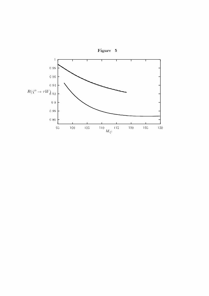
Figure 5

0.86

0.88

0.9

0.92

0.94

0.96

0.98

1

95 100 105 110 115 120 125 130

B(~

0

! W )

M

~

0

Figure 6

0.6

0.65

0.7

0.75

0.8

0.85

0.9

0.95

1

100 105 110 115 120 125 130 135 140 145

B(~

0

!

Z)

M

~

0