Chapter 3. Bilinear formsLecture notes for MA1212

P. Karageorgis

pete@maths.tcd.ie

1 / 25

Bilinear forms

Definition 3.1 – Bilinear form

A bilinear form on a real vector space V is a function f : V × V → R

which assigns a number to each pair of elements of V in such a way

that f is linear in each variable.

A typical example of a bilinear form is the dot product on Rn.

We shall usually write 〈x,y〉 instead of f(x,y) for simplicity and we

shall also identify each 1× 1 matrix with its unique entry.

Theorem 3.2 – Bilinear forms on Rn

Every bilinear form on Rn has the form

〈x,y〉 = xtAy =∑

i,j

aijxiyj

for some n× n matrix A and we also have aij = 〈ei, ej〉 for all i, j.2 / 25

Matrix of a bilinear form

Definition 3.3 – Matrix of a bilinear form

Suppose that 〈 , 〉 is a bilinear form on V and let v1,v2, . . . ,vn be a

basis of V . The matrix of the form with respect to this basis is the

matrix A whose entries are given by aij = 〈vi,vj〉 for all i, j.

Theorem 3.4 – Change of basis

Suppose that 〈 , 〉 is a bilinear form on Rn and let A be its matrix with

respect to the standard basis. Then the matrix of the form with respect

to some other basis v1,v2, . . . ,vn is given by BtAB, where B is the

matrix whose columns are the vectors v1,v2, . . . ,vn.

There is a similar result for linear transformations: if A is the matrix

with respect to the standard basis and v1,v2, . . . ,vn is some other

basis, then the matrix with respect to the other basis is B−1AB.

3 / 25

Matrix of a bilinear form: Example

Let P2 denote the space of real polynomials of degree at most 2.Then P2 is a vector space and its standard basis is 1, x, x2.

We can define a bilinear form on P2 by setting

〈f, g〉 =∫

1

0

f(x)g(x) dx for all f, g ∈ P2.

By definition, the matrix of a form with respect to a given basis has

entries aij = 〈vi,vj〉. In our case, vi = xi−1 for each i and so

aij =⟨

xi−1, xj−1⟩

=

∫

1

0

xi+j−2 dx =1

i+ j − 1.

Thus, the matrix of the form with respect to the standard basis is

A =

1 1/2 1/31/2 1/3 1/41/3 1/4 1/5

.

4 / 25

Positive definite forms

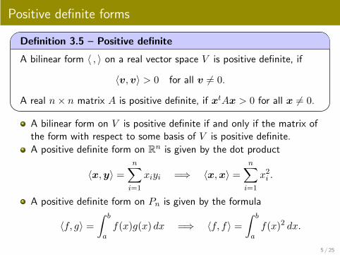
Definition 3.5 – Positive definite

A bilinear form 〈 , 〉 on a real vector space V is positive definite, if

〈v,v〉 > 0 for all v 6= 0.

A real n× n matrix A is positive definite, if xtAx > 0 for all x 6= 0.

A bilinear form on V is positive definite if and only if the matrix of

the form with respect to some basis of V is positive definite.

A positive definite form on Rn is given by the dot product

〈x,y〉 =n∑

i=1

xiyi =⇒ 〈x,x〉 =n∑

i=1

x2i .

A positive definite form on Pn is given by the formula

〈f, g〉 =∫ b

a

f(x)g(x) dx =⇒ 〈f, f〉 =∫ b

a

f(x)2 dx.

5 / 25

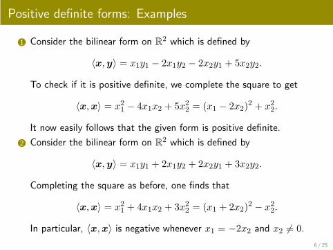
Positive definite forms: Examples

1 Consider the bilinear form on R2 which is defined by

〈x,y〉 = x1y1 − 2x1y2 − 2x2y1 + 5x2y2.

To check if it is positive definite, we complete the square to get

〈x,x〉 = x21 − 4x1x2 + 5x22 = (x1 − 2x2)2 + x22.

It now easily follows that the given form is positive definite.

2 Consider the bilinear form on R2 which is defined by

〈x,y〉 = x1y1 + 2x1y2 + 2x2y1 + 3x2y2.

Completing the square as before, one finds that

〈x,x〉 = x21 + 4x1x2 + 3x22 = (x1 + 2x2)2 − x22.

In particular, 〈x,x〉 is negative whenever x1 = −2x2 and x2 6= 0.

6 / 25

Symmetric forms

Definition 3.6 – Symmetric

A bilinear form 〈 , 〉 on a real vector space V is called symmetric, if

〈v,w〉 = 〈w,v〉 for all v,w ∈ V .

A real square matrix A is called symmetric, if aij = aji for all i, j.

A bilinear form on V is symmetric if and only if the matrix of the

form with respect to some basis of V is symmetric.

A real square matrix A is symmetric if and only if At = A.

Definition 3.7 – Inner product

An inner product on a real vector space V is a bilinear form which is

both positive definite and symmetric.

7 / 25

Angles and length

Suppose that 〈 , 〉 is an inner product on a real vector space V .

Then one may define the length of a vector v ∈ V by setting

||v|| =√

〈v,v〉

and the angle θ between two vectors v,w ∈ V by setting

cos θ =〈v,w〉

||v|| · ||w|| .

These formulas are known to hold for the inner product on Rn.

Theorem 3.8 – Cauchy-Schwarz inequality

When V is a real vector space with an inner product, one has

| 〈v,w〉 | ≤ ||v|| · ||w|| for all v,w ∈ V .

8 / 25

Orthogonal vectors

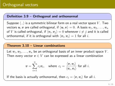
Definition 3.9 – Orthogonal and orthonormal

Suppose 〈 , 〉 is a symmetric bilinear form on a real vector space V . Two

vectors u,v are called orthogonal, if 〈u,v〉 = 0. A basis v1,v2, . . . ,vnof V is called orthogonal, if 〈vi,vj〉 = 0 whenever i 6= j and it is called

orthonormal, if it is orthogonal with 〈vi,vi〉 = 1 for all i.

Theorem 3.10 – Linear combinations

Let v1,v2, . . . ,vn be an orthogonal basis of an inner product space V .

Then every vector v ∈ V can be expressed as a linear combination

v =n∑

i=1

civi, where ci =〈v,vi〉〈vi,vi〉

for all i.

If the basis is actually orthonormal, then ci = 〈v,vi〉 for all i.

9 / 25

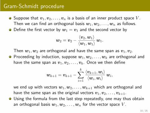
Gram-Schmidt procedure

Suppose that v1,v2, . . . ,vn is a basis of an inner product space V .

Then we can find an orthogonal basis w1,w2, . . . ,wn as follows.

Define the first vector by w1 = v1 and the second vector by

w2 = v2 −〈v2,w1〉〈w1,w1〉

w1.

Then w1,w2 are orthogonal and have the same span as v1,v2.

Proceeding by induction, suppose w1,w2, . . . ,wk are orthogonal and

have the same span as v1,v2, . . . ,vk. Once we then define

wk+1 = vk+1 −k

∑

i=1

〈vk+1,wi〉〈wi,wi〉

wi,

we end up with vectors w1,w2, . . . ,wk+1 which are orthogonal and

have the same span as the original vectors v1,v2, . . . ,vk+1.

Using the formula from the last step repeatedly, one may thus obtain

an orthogonal basis w1,w2, . . . ,wn for the vector space V .

10 / 25

Gram-Schmidt procedure: Example

We find an orthogonal basis of R3, starting with the basis

v1 =

101

, v2 =

111

, v3 =

123

.

We define the first vector by w1 = v1 and the second vector by

w2 = v2 −〈v2,w1〉〈w1,w1〉

w1 =

111

− 2

2

101

=

010

.

Then w1,w2 are orthogonal and we may define the third vector by

w3 = v3 −〈v3,w1〉〈w1,w1〉

w1 −〈v3,w2〉〈w2,w2〉

w2

=

123

− 4

2

101

− 2

1

010

=

−101

.

11 / 25

Bilinear forms over a complex vector space

Bilinear forms are defined on a complex vector space in the same way

that they are defined on a real vector space. However, one needs to

conjugate one of the variables to ensure positivity of the dot product.

The complex transpose of a matrix is denoted by A∗ = At and it is

also known as the adjoint of A. One has x∗x ≥ 0 for all x ∈ Cn.

Bilinear forms on Rn Bilinear forms on C

n

Linear in the first variable Conjugate linear in the first variable

〈u+ v,w〉 = 〈u,w〉+ 〈v,w〉 〈u+ v,w〉 = 〈u,w〉+ 〈v,w〉〈λu,v〉 = λ 〈u,v〉 〈λu,v〉 = λ 〈u,v〉

Linear in the second variable Linear in the second variable

〈x,y〉 = xtAy for some A 〈x,y〉 = x∗Ay for some A

Symmetric, if At = A Hermitian, if A∗ = A

Symmetric, if aij = aji Hermitian, if aij = aji

12 / 25

Real symmetric matrices

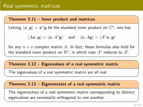
Theorem 3.11 – Inner product and matrices

Letting 〈x,y〉 = x∗y be the standard inner product on Cn, one has

〈Ax,y〉 = 〈x, A∗y〉 and 〈x, Ay〉 = 〈A∗x,y〉

for any n × n complex matrix A. In fact, these formulas also hold for

the standard inner product on Rn, in which case A∗ reduces to At.

Theorem 3.12 – Eigenvalues of a real symmetric matrix

The eigenvalues of a real symmetric matrix are all real.

Theorem 3.13 – Eigenvectors of a real symmetric matrix

The eigenvectors of a real symmetric matrix corresponding to distinct

eigenvalues are necessarily orthogonal to one another.

13 / 25

Orthogonal matrices

Definition 3.14 – Orthogonal matrix

A real n× n matrix A is called orthogonal, if AtA = In.

Theorem 3.15 – Properties of orthogonal matrices

1 To say that an n× n matrix A is orthogonal is to say that the

columns of A form an orthonormal basis of Rn.

2 The product of two n× n orthogonal matrices is orthogonal.

3 Left multiplication by an orthogonal matrix preserves both angles

and length. When A is an orthogonal matrix, that is, one has

〈Ax, Ay〉 = 〈x,y〉 and ||Ax|| = ||x||.

An example of a 2× 2 orthogonal matrix is A =

[

cos θ − sin θsin θ cos θ

]

.

14 / 25

Spectral theorem

Theorem 3.16 – Spectral theorem

Every real symmetric matrix A is diagonalisable. In fact, there exists

an orthogonal matrix B such that B−1AB = BtAB is diagonal.

When the eigenvalues of A are distinct, the eigenvectors of A are

orthogonal and we may simply divide each of them by its length to

obtain an orthonormal basis of Rn. Such a basis can be merged to

form an orthogonal matrix B such that B−1AB is diagonal.

When the eigenvalues of A are not distinct, the eigenvectors of Amay not be orthogonal. In that case, one may use the Gram-Schmidt

procedure to replace eigenvectors that have the same eigenvalue with

orthogonal eigenvectors that have the same eigenvalue.

The converse of the spectral theorem is also true. That is, if B is an

orthogonal matrix and BtAB is diagonal, then A is symmetric.

15 / 25

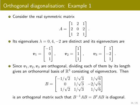
Orthogonal diagonalisation: Example 1

Consider the real symmetric matrix

A =

1 2 12 0 21 2 1

.

Its eigenvalues λ = 0, 4,−2 are distinct and its eigenvectors are

v1 =

−101

, v2 =

111

, v3 =

1−21

.

Since v1,v2,v3 are orthogonal, dividing each of them by its length

gives an orthonormal basis of R3 consisting of eigenvectors. Then

B =

−1/√2 1/

√3 1/

√6

0 1/√3 −2/

√6

1/√2 1/

√3 1/

√6

is an orthogonal matrix such that B−1AB = BtAB is diagonal.

16 / 25

Orthogonal diagonalisation: Example 2

Consider the real symmetric matrix

A =

2 1 11 2 11 1 2

.

Its eigenvalues are λ = 1, 1, 4 and its eigenvectors are

v1 =

−101

, v2 =

−110

, v3 =

111

.

In this case, we use the Gram-Schmidt procedure to replace v1,v2 by

two orthogonal eigenvectors w1,w2. Dividing each of w1,w2,v3 by

its length, we then obtain the columns of the orthogonal matrix

B =

−1/√2 −1/

√6 1/

√3

0 2/√6 1/

√3

1/√2 −1/

√6 1/

√3

.

17 / 25

Quadratic forms

Definition 3.17 – Quadratic form

A quadratic form in n variables is a function that has the form

Q(x1, x2, . . . , xn) =∑

i≤j

aijxixj .

This can be written as Q(x) = xtAx for some symmetric matrix A.

Here, one needs to be careful with the off-diagonal entries aij , as thecoefficient of xixj needs to be halved whenever i 6= j. For instance,

Q(x) = x21 + 4x1x2 + 3x22 = xtAx, A =

[

1 22 3

]

.

The most general quadratic function in n variables has the form

Q(x) =∑

i≤j

aijxixj +∑

k

bkxk + c = xtAx+ btx+ c.

18 / 25

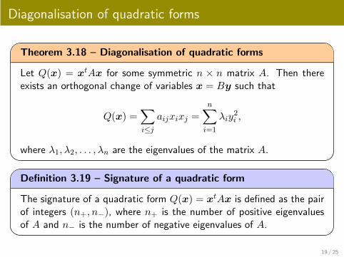
Diagonalisation of quadratic forms

Theorem 3.18 – Diagonalisation of quadratic forms

Let Q(x) = xtAx for some symmetric n × n matrix A. Then there

exists an orthogonal change of variables x = By such that

Q(x) =∑

i≤j

aijxixj =n∑

i=1

λiy2i ,

where λ1, λ2, . . . , λn are the eigenvalues of the matrix A.

Definition 3.19 – Signature of a quadratic form

The signature of a quadratic form Q(x) = xtAx is defined as the pair

of integers (n+, n−), where n+ is the number of positive eigenvalues

of A and n− is the number of negative eigenvalues of A.

19 / 25

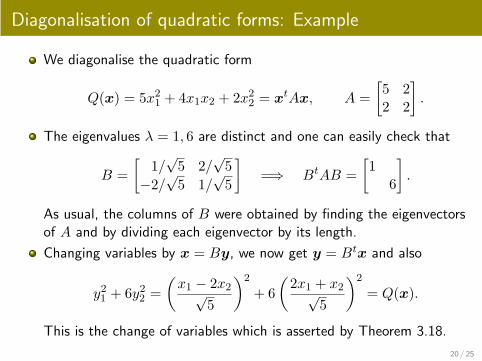
Diagonalisation of quadratic forms: Example

We diagonalise the quadratic form

Q(x) = 5x21 + 4x1x2 + 2x22 = xtAx, A =

[

5 22 2

]

.

The eigenvalues λ = 1, 6 are distinct and one can easily check that

B =

[

1/√5 2/

√5

−2/√5 1/

√5

]

=⇒ BtAB =

[

16

]

.

As usual, the columns of B were obtained by finding the eigenvectors

of A and by dividing each eigenvector by its length.

Changing variables by x = By, we now get y = Btx and also

y21 + 6y22 =

(

x1 − 2x2√5

)2

+ 6

(

2x1 + x2√5

)2

= Q(x).

This is the change of variables which is asserted by Theorem 3.18.

20 / 25

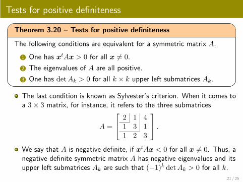
Tests for positive definiteness

Theorem 3.20 – Tests for positive definiteness

The following conditions are equivalent for a symmetric matrix A.

1 One has xtAx > 0 for all x 6= 0.

2 The eigenvalues of A are all positive.

3 One has detAk > 0 for all k × k upper left submatrices Ak.

The last condition is known as Sylvester’s criterion. When it comes to

a 3× 3 matrix, for instance, it refers to the three submatrices

A =

2 1 41 3 11 2 3

.

We say that A is negative definite, if xtAx < 0 for all x 6= 0. Thus, anegative definite symmetric matrix A has negative eigenvalues and its

upper left submatrices Ak are such that (−1)k detAk > 0 for all k.

21 / 25

Sylvester’s criterion: Example

Let a be a real parameter and consider the matrix

A =

a 1 11 1 a1 a 5

.

By Sylvester’s criterion, A is positive definite if and only if

a > 0, det

[

a 11 1

]

> 0, detA > 0.

The first two conditions give a > 0 and a > 1, while

detA = −a3 + 7a− 6 = −(a− 1)(a− 2)(a+ 3).

It easily follows that A is positive definite if and only if 1 < a < 2.

22 / 25

Application 1: Second derivative test

Given a function f(x, y) of two variables, its directional derivative in

the direction of a unit vector u is given by Duf = u1fx + u2fy.

In particular, the second derivative of f in the direction of u is

DuDuf = u1(u1fx + u2fy)x + u2(u1fx + u2fy)y

= u21fxx + u1u2fyx + u2u1fxy + u22fyy = utAu.

This computation allows us to classify the critical points of f . If thesecond derivative is positive for all u 6= 0, then the function is convex

in all directions and we get a local minimum. If the second derivative

is negative for all u 6= 0, then we get a local maximum.

To classify the critical points, one looks at the Hessian matrix

A =

[

fxx fyxfxy fyy

]

.

This is symmetric, so it is diagonalisable with real eigenvalues. Once

we now consider three cases, we obtain the second derivative test.

23 / 25

Application 2: Min/Max value on the unit sphere

Let A be a symmetric n× n matrix and consider the quadratic form

Q(x) =∑

i≤j

aijxixj = xtAx.

To find the minimum value of Q(x) on the unit sphere ||x|| = 1, welet B be an orthogonal matrix such that BtAB is diagonal and then

use the orthogonal change of variables x = By to write

Q(x) =n∑

i=1

λi y2i .

Since ||y|| = ||By|| = ||x|| = 1 by orthogonality, we find that

Q(x) =n∑

i=1

λi y2i ≥

n∑

i=1

λmin y2i = λmin.

In particular, minQ(x) is the smallest eigenvalue of A, while a similar

argument shows that maxQ(x) is the largest eigenvalue of A.

24 / 25

Application 3: Min/Max value of quadratics

Every quadratic function of n variables can be expressed in the form

Q(x) =∑

i≤j

aijxixj +∑

k

bkxk + c = xtAx+ xtb+ c.

Suppose A is positive definite symmetric and let x0 = −1

2A−1b. Then

Q(x0) = xt0Ax0 + xt

0b+ c = −xt0Ax0 + c

is the minimum value that is attained by the quadratic because

0 ≤ (x− x0)tA(x− x0) = xtAx− 2xtAx0 + xt

0Ax0

= xtAx+ xtb+ c−Q(x0)

= Q(x)−Q(x0).

When A is negative definite symmetric, the inequality is reversed and

thus Q(x0) is the maximum value that is attained by the quadratic.

25 / 25