Seismic active earth pressure on bilinear retaining walls using a modified pseudo‑dynamic methodObaidur Rahaman1,2 and Prishati Raychowdhury2*

Abstract

Background: Proper understanding of seismic behavior of retaining structures is crucial during a strong earthquake event. In particular, response of retaining walls with bilinear backface, where a sudden change in the inclination along its depth make the problem more complex. This study focuses on estimating the seismic earth pressure coefficients of a retaining wall with bilinear backface using a modified pseudo-dynamic method.

Methods: In this method, the backfill soil is modeled as a visco-elastic Kelvin–Voigt material. A frequency-dependant amplification function is derived for the waves traveling along the backfill using well-established one-dimensional ground response analysis theory. A rigorous parametric study has been carried out to understand the effect of various parameters such as amplitude of base acceleration, direction of verti-cal acceleration, soil shear resistance angle, soil-wall friction angle, wall inclination, frequency ratio, and damping ratio on the seismic active earth pressure.

Results: It has been observed that the damping ratio of the backfill soil plays an important role, particularly when the frequency of wave is close to the natural fre-quency of the backfill. Further, the seismic active thrust is found to increase in both upper and lower segments of the wall when the frequency of the primary wave is greater than that of the shear wave. Comparison of results with the previous studies indicates that the conventional pseudo-dynamic methods significantly underesti-mate the seismic coefficients and seismic pressures, particularly for the high-intensity motions.

Conclusions: The results of the study show that the natural frequency and damping of the backfill soil have significant effect on the seismic active earth pressure coef-ficients. Comparison with conventional pseudo-static and pseudo-dynamic methods indicates that the previous methods largely underestimate seismic coefficients and seismic pressures (as much as 48%). This under-estimation is more prominent for higher-intensity motions and less-damped soil, where the soil amplification effects pose most importance. This modified pseudo-dynamic approach can further be used for design of bilinear retaining structures.

Keywords: Pseudo-dynamic method, Bilinear retaining wall, Active earth pressure, Seismic behavior, Soil amplification

Open Access

© The Author(s) 2017. This article is distributed under the terms of the Creative Commons Attribution 4.0 International License (http://creativecommons.org/licenses/by/4.0/), which permits unrestricted use, distribution, and reproduction in any medium, provided you give appropriate credit to the original author(s) and the source, provide a link to the Creative Commons license, and indicate if changes were made.

RESEARCH

Rahaman and Raychowdhury Geo-Engineering (2017) 8:6 DOI 10.1186/s40703‑017‑0040‑4

*Correspondence: prishati@iitk.ac.in 2 Department of Civil Engineering, Indian Institute of Technology Kanpur, Kanpur, IndiaFull list of author information is available at the end of the article

Page 2 of 24Rahaman and Raychowdhury Geo-Engineering (2017) 8:6

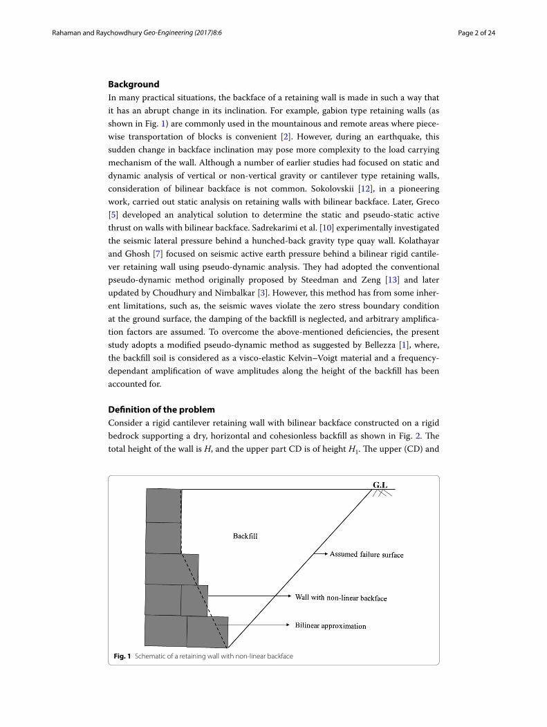
BackgroundIn many practical situations, the backface of a retaining wall is made in such a way that it has an abrupt change in its inclination. For example, gabion type retaining walls (as shown in Fig. 1) are commonly used in the mountainous and remote areas where piece-wise transportation of blocks is convenient [2]. However, during an earthquake, this sudden change in backface inclination may pose more complexity to the load carrying mechanism of the wall. Although a number of earlier studies had focused on static and dynamic analysis of vertical or non-vertical gravity or cantilever type retaining walls, consideration of bilinear backface is not common. Sokolovskii [12], in a pioneering work, carried out static analysis on retaining walls with bilinear backface. Later, Greco [5] developed an analytical solution to determine the static and pseudo-static active thrust on walls with bilinear backface. Sadrekarimi et al. [10] experimentally investigated the seismic lateral pressure behind a hunched-back gravity type quay wall. Kolathayar and Ghosh [7] focused on seismic active earth pressure behind a bilinear rigid cantile-ver retaining wall using pseudo-dynamic analysis. They had adopted the conventional pseudo-dynamic method originally proposed by Steedman and Zeng [13] and later updated by Choudhury and Nimbalkar [3]. However, this method has from some inher-ent limitations, such as, the seismic waves violate the zero stress boundary condition at the ground surface, the damping of the backfill is neglected, and arbitrary amplifica-tion factors are assumed. To overcome the above-mentioned deficiencies, the present study adopts a modified pseudo-dynamic method as suggested by Bellezza [1], where, the backfill soil is considered as a visco-elastic Kelvin–Voigt material and a frequency-dependant amplification of wave amplitudes along the height of the backfill has been accounted for.

Definition of the problemConsider a rigid cantilever retaining wall with bilinear backface constructed on a rigid bedrock supporting a dry, horizontal and cohesionless backfill as shown in Fig. 2. The total height of the wall is H, and the upper part CD is of height H1. The upper (CD) and

Fig. 1 Schematic of a retaining wall with non-linear backface

Page 3 of 24Rahaman and Raychowdhury Geo-Engineering (2017) 8:6

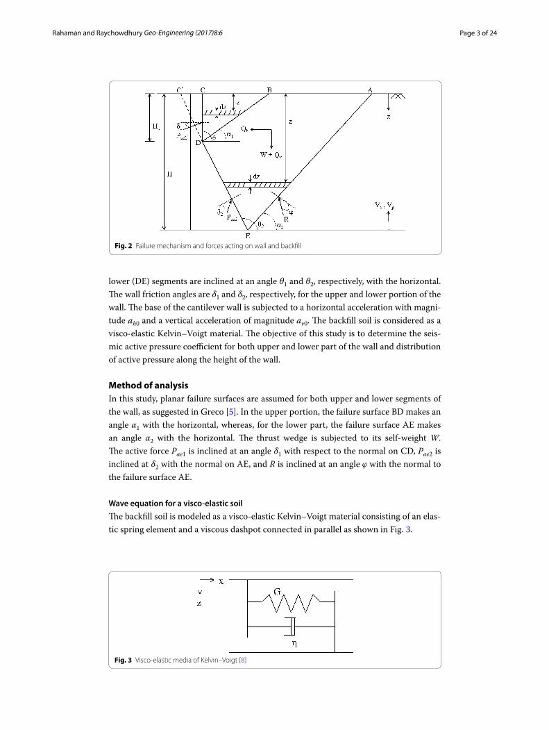
lower (DE) segments are inclined at an angle θ1 and θ2, respectively, with the horizontal. The wall friction angles are δ1 and δ2, respectively, for the upper and lower portion of the wall. The base of the cantilever wall is subjected to a horizontal acceleration with magni-tude ah0 and a vertical acceleration of magnitude av0. The backfill soil is considered as a visco-elastic Kelvin–Voigt material. The objective of this study is to determine the seis-mic active pressure coefficient for both upper and lower part of the wall and distribution of active pressure along the height of the wall.

Method of analysisIn this study, planar failure surfaces are assumed for both upper and lower segments of the wall, as suggested in Greco [5]. In the upper portion, the failure surface BD makes an angle α1 with the horizontal, whereas, for the lower part, the failure surface AE makes an angle α2 with the horizontal. The thrust wedge is subjected to its self-weight W. The active force Pae1 is inclined at an angle δ1 with respect to the normal on CD, Pae2 is inclined at δ2 with the normal on AE, and R is inclined at an angle ϕ with the normal to the failure surface AE.

Wave equation for a visco‑elastic soil

The backfill soil is modeled as a visco-elastic Kelvin–Voigt material consisting of an elas-tic spring element and a viscous dashpot connected in parallel as shown in Fig. 3.

Fig. 2 Failure mechanism and forces acting on wall and backfill

Fig. 3 Visco-elastic media of Kelvin–Voigt [8]

Page 4 of 24Rahaman and Raychowdhury Geo-Engineering (2017) 8:6

According to the definition of Kelvin–Voigt model, the constitutive equation of a visco-elastic medium is given by

where σxz is the shear stress, ɛxz is the shear strain, G is the shear modulus and η is the viscous damping coefficient. For a harmonic shaking, ηs = 2GD/ω, where D is damping ratio and w is angular frequency. The motion equation of the Kelvin–Voigt visco-elastic medium (after [14]) is

where ρ is the density of the media, λ and G are the Lame constant, η1 and ηs are the vis-cosities, u is displacement vector with components along three different axis ux, uy and uz, and θ = div(u). If the plane wave solution of wave propagating along the z-axis in the Kelvin–Voigt homogeneous visco-elastic medium is considered, then Eq. (2) can be sim-plified as the following two equations for horizontal and vertical displacement vectors:

and

The general solution of Eq. (3) for a harmonic wave is

where k∗s is complex wave number defined as

where G∗ is complex shear modulus and given by

By applying the boundary conditions that is shear stress at the free surface (z = 0) is zero and at z = H the displacement will be equal to the rigid base (ubh = uh0 exp(iωt)), the horizontal displacement is expressed as

Taking only the real part, Eq. (8) can be expressed as

(1)σxz = 2Gεxz + 2η∂εxz

∂t

(2)ρ∂2u

∂t2=

{

(�+ G)+ (η1 + ηs)∂

∂t

}

grad(θ)+

(

G + ηs∂

∂t

)

∇2u

(3)ρ∂2uh

∂t2= G

∂2uh

∂z2+ ηs

∂3uh

∂t∂z2

(4)ρ∂2uv

∂t2= (�+ 2G)

∂2uv

∂z2+ (η1 + 2ηs)

∂3uv

∂t∂z2

(5)uh(z, t) = exp(iωt){

C1 exp(

−ik∗s z)

+ C2 exp(

ik∗s z)}

(6)k∗s = ωs

√

ρ/

G∗ = ks1 + iks2

(7)G∗= G + iωηs = G(1+ 2Dsi)

(8)uh(z, t) = uh0 exp(iωt)cos

(

k∗s z)

cos(

k∗s H)

(9)uh(z, t) =uh0

C2s + S2s

[(CsCsz + SsSsz) cos (wst)+ (SsCsz − CsSsz) sin (wst)]

Page 5 of 24Rahaman and Raychowdhury Geo-Engineering (2017) 8:6

The horizontal acceleration can be obtained

Similarly, the vertical acceleration is obtained as

where

(10)ah(z, t) =ah0

C2s + S2s

[(CsCsz + SsSsz) cos (wst)+ (SsCsz − CsSsz) sin (wst)]

(11)av(z, t) =av0

C2p + S2p

[(

CpCpz + SpSpz)

cos(

wpt)

+(

SpCpz + CpSpz)

sin(

wpt)]

Csz = cos(

ys1z/H)

cosh(

ys2z/H)

Cpz = cos(

yp1z/H)

cosh(

yp2z/H)

Ssz = − sin(

ys1z/H)

sinh(

ys2z/H)

Spz = − sin(

yp1z/H)

sinh(

yp2z/H)

Cs = cos(

ys1)

cosh(

ys2)

Cp = cos(

yp1)

cosh(

yp2)

Ss = − sin(

ys1)

sinh(

ys2)

Sp = − sin(

yp1)

sinh(

yp2)

ys1 = ks1H =wsH

Vs

√

√

1+ 4D2s + 1

2(

1+ 4D2s

)

yp1 = kp1H =wpH

Vp

√

√

√

√

√

√

1+ 4D2p + 1

2(

1+ 4D2p

)

ys2 = ks2H = −wsH

Vs

√

√

1+ 4D2s − 1

2(

1+ 4D2s

)

yp2 = kp2H = −wpH

Vp

√

√

√

√

√

√

1+ 4D2p − 1

2(

1+ 4D2p

)

Page 6 of 24Rahaman and Raychowdhury Geo-Engineering (2017) 8:6

where ks1 and ks2 are the real and imaginary parts of complex wave number k∗s , kp1 and kp2 real and imaginary parts of k∗p, is the first Lame’s constant, Ds and Dp are damping ratios and ωp and ωs are angular frequencies for shear and primary wave, respectively.

Estimation of active thrust for the upper segment (CD)

To estimate the active earth pressure on the upper segment, the equilibrium of the soil wedge BCD has been considered. The mass of the thin element of thickness dz at depth z in wedge BCD is given by

where γ is unit weight of the backfill soil and g is acceleration due to gravity. The total weight of wedge BCD is computed by integrating Eq. (12) as

The total horizontal inertial force (Qh1) and vertical inertial force (Qv1) on the wedge BCD are given by

The total horizontal inertial force (Qh1) and vertical inertial force (Qv1) can be expressed as

where the dimensionless coefficients Ahu, Bhu, Avu and Bvu are given by

(12)m1(z) =γ

g(H1 − z)(cot α1 − cot θ1)dz

(13)W1 =

H1∫

0

m1(z)dz =γH2

1

2(cot α1 − cot θ1)

(14)Qh1(t,α1) =

z=H1∫

z=0

ah(z, t)m(z) =

z=H1∫

z=0

ah(z, t)γ

g(H1 − z)(cot α1 − cot θ1)dz

(15)Qv1(t,α1) =

z=H1∫

z=0

αv(z, t)m(z) =

z=H1∫

z=0

αv(z, t)γ

g(H1 − z)(cot α1 − cot θ1)dz

(16)Qh1(t,α1) =ah0

gγH2

1 (cot α1 − cot θ1)[Ahu cos (wst)+ Bhu sin (wst)]

(17)Qv1(t,α1) =av0

gγH2

1 (cot α1 − cot θ1)[

Avu cos(

wpt)

+ Bvu sin(

wpt)]

Ahu =

2ys1uys2u sin(

ys1u)

sinh(

ys2u)

+(

y2s1u − y2s2u)

{

cos(

ys1u)

cosh(

ys2u)

− cos2(

ys1u)

− sinh2(

ys2u)

}

{

cos2(

ys1u)

+ sinh2(

ys2u)

}

(

y2s1u + y2s2u)2

Bhu =

2ys1uys2u

{

cos(

ys1u)

cosh(

ys2u)

− cos2(

ys1u)

− sinh2(

ys2u)

}

−(

y2s1u − y2s2u)

sin(

ys1u)

sinh(

ys2u)

{

cos2(

ys1u)

+ sinh2(

ys2u)

}

(

y2s1u + y2s2u)2

Page 7 of 24Rahaman and Raychowdhury Geo-Engineering (2017) 8:6

also ys1u = ks1H1, ys2u = ks2H1, yp1u = kp1H1 and yp2u = kp2H1.Assuming the wedge BCD is in limit equilibrium condition and considering the verti-

cal and horizontal equilibrium of the wedge, the total active thrust on the upper portion of the wall is obtained using the following equation

The maximum value of Eq. (18) with respect to α1 and t can be considered as the esti-mated seismic active pressure on the wall. Substituting Eqs. (13), (16) and (17) in Eq. (18)

The seismic active earth pressure coefficient can be obtained by the following equation

where α1m and tm are the values of α1 and t that maximizes Kae1.

Estimation of active thrust for the lower segment (DE)

For determination of active pressure on the lower part,the contribution of the entire wedge ABCDE has to be considered. The mass of the thin element of thickness dz at depth z in wedge ABCDE as shown in Fig. 2 is given by

where m21(z) is the mass of wedge ABC′DE, expressed as

and m22(z) which is the mass of wedge CC′D, is given by

Avu =

2yp1uyp2u sin(

yp1u)

sinh(

yp2u)

+

(

y2p1u − y2p2u

){

cos(

yp1u)

cosh(

yp2u)

− cos2(

yp1u)

− sinh2(

yp2u)

}

{

cos2(

yp1u)

+ sinh2(

yp2u)

}(

y2p1u + y2p2u

)2

Bvu =

2yp1uyp2u

{

cos(

yp1u)

cosh(

yp2u)

− cos2(

yp1u)

− sinh2(

yp2u)

}

−

(

y2p1u − y2p2u

)

sin(

yp1u)

sinh(

yp2u)

{

cos2(

yp1u)

+ sinh2(

yp2u)

}(

y2p1u + y2p2u

)2

(18)Pae1(α1, t) =W1 sin (α1 − ϕ)

sin (δ1 + θ1 + ϕ − α1)+

Qh1 cos (α1 − ϕ)+ Qv1 sin (α1 − ϕ)

sin (δ1 + θ1 + ϕ − α1)

(19)Pae1,max = max

γH21

2

sin (α1−ϕ)(cot α1−cot θ1)sin (δ1+θ1+ϕ−α1)

+ah0g γH2

1

cos (α1−ϕ)(cot α1−cot θ1)sin (δ1+θ1+ϕ−α1)

[Ahu cos (wst)+ Bhu sin (wst)]

+av0g γH2

1

sin (α1−ϕ)(cot α1−cot θ1)sin (δ1+θ1+ϕ−α1)

�

Avu cos�

wpt�

+ Bvu sin�

wpt��

(20)

Kae1 =2Pae1,max

γH21

=

sin (α1m−ϕ)(cot α1m−cot θ1)sin (δ1+θ1+ϕ−α1m)

+2ah0g

cos (α1m−ϕ)(cot α1m−cot θ1)sin (δ1+θ1+ϕ−α1m)

[Ahu cos (wstm)+ Bhu sin (wstm)]

+2av0g

sin (α1m−ϕ)(cot α1m−cot θ1)sin (δ1+θ1+ϕ−α1m)

�

Avu cos�

wptm�

+ Bvu sin�

wptm��

(21)m2(z) = m21(z)−m22(z)

(22)m21(z) =γ

g(H − z)(cot α2 − cot θ2)dz 0 ≤ z ≤ H

(23)m22(z) =γ

g(H1 − z)(cot θ1 − cot θ2)dz 0 ≤ z ≤ H1

Page 8 of 24Rahaman and Raychowdhury Geo-Engineering (2017) 8:6

The total weight of wedge ABCDE can be derived as

The total horizontal inertial force (Qh2) and vertical inertial force (Qv2) on the wedge ABCDE are given by

The total active thrust on the lower portion of the wall is obtained by imposing the vertical and horizontal equilibrium of the wedge ABCDE, assuming the wedge is in limit equilibrium condition and it is expressed as

Also, the seismic active earth pressure coefficient for the lower portion can be obtained by the following equation

Estimation of active earth pressure distribution

The seismic active earth pressure distribution can be obtained by writing Pae1 and Pae2 as functions of z instead of H, and then partially differentiating them with respect to z [13]. By normalizing active pressure distribution (pae1) along the upper segment with respect to γH, pae1

γH is expressed as

where,

(24)W2 =

z=H∫

z=0

m21(z)−

z=H1∫

z=0

m22(z) =γ

2

[

H2(cot α2 − cot θ2)−H21 (cot θ1 − cot θ2)

]

(25)Qh2(t,α2) =

z=H∫

z=0

ah(z, t)m21(z)−

z=H1∫

z=0

ah(z, t)m22(z)

(26)Qv2(t,α2) =

z=H∫

z=0

αv(z, t)m21(z)−

z=H1∫

z=0

αv(z, t)m22(z)

(27)Pae2(α2, t) =

W2 sin (α2−ϕ)sin (δ2+θ2+ϕ−α2)

+Qh2 cos (α2−ϕ)+Qv2 sin (α2−ϕ)

sin (δ2+θ2+ϕ−α2)

−Pae1(α1,t) sin (δ1+θ1+ϕ−α2)

sin (δ2+θ2+ϕ−α2)

(28)Kae2 =2Pae2,max

γH2

(29)pae1

γH=

zH (cot α1 − cot θ1)

sin (α1−ϕ)sin (δ1+θ1+ϕ−α1)

+ah0g (cot α1 − cot θ1)

�

Aph cos (ωst)+ Bph sin (ωst)�

cos (α1−ϕ)sin (δ1+θ1+ϕ−α1)

+av0g (cot α1 − cot θ1)

�

Apv cos�

ωpt�

+ Bpv sin�

ωpt��

sin (α1−ϕ)sin (δ1+θ1+ϕ−α1)

Aph =

(

Csys2 + Ssys1)

cos(

ys1zH

)

sinh(

ys2zH

)

+(

Csys1 − Ssys2)

sin(

ys1zH

)

cosh(

ys2zH

)

(

C2s + S2s

)(

y2s1 + y2s2)

Bph =

(

Ssys2 − Csys1)

cos(

ys1zH

)

sinh(

ys2zH

)

+(

Ssys1 + Csys2)

sin(

ys1zH

)

cosh(

ys2zH

)

(

C2s + S2s

)(

y2s1 + y2s2)

Page 9 of 24Rahaman and Raychowdhury Geo-Engineering (2017) 8:6

Similarly, for the lower segment, the normalized active earth pressure distribution is expressed as

where,

Results and discussionThe maximum seismic active earth pressure coefficients for both upper and lower seg-ments have been determined by optimizing Eq. (20) and (28) with respect to α1, α2 and t/T. In this analysis, the damping ratio of soil during propagation of shear wave and pri-mary wave are assumed to be same, i.e., Ds = Dp = D. Further, the soil-wall friction angle for both upper and lower segments are assumed to be equal, i.e. δ1 = δ2 = δ. Poisson’s ratio of the backfill soil is assumed as 0.3, which gives the ratio of P-wave and S-wave velocity (Vp/Vs) approximately 1.87 [4, 8]. The effect of various parameters are investi-gated on three response parameters, namely, seismic active earth pressure coefficients, seismic earth pressure distribution over the height of the wall, and failure angle. Note that the damping ratio of 10% is assumed in the present analysis. Further, to under-stand the effect of damping on the earth pressure, additional analyses with 10, 20 and

Apv =

(

Cpyp2 + Spyp1)

cos(

yp1zH

)

sinh(

yp2zH

)

+(

Cpyp1 − Spyp2)

sin(

yp1zH

)

cosh(

yp2zH

)

(

C2p + S2p

)(

y2p1 + y2p2

)

Bpv =

(

Spyp2 − Cpyp1)

cos(

yp1zH

)

sinh(

yp2zH

)

+(

Spyp1 + Cpyp2)

sin(

yp1zH

)

cosh(

yp2zH

)

(

C2p + S2p

)(

y2p1 + y2p2

)

(30)pae2

γH=

�

z

H(cot α2 − cot θ2)−

H1

H(cot θ1 − cot θ2)

�

sin (α2 − ϕ)

sin (δ2 + θ2 + ϕ − α2)

+αh0

g

�

(cot α2 − cot θ2)�

Aph cos (ωst)+ Bph sin (ωst)�

(cot θ1 − cot θ2)�

Cph cos (ωst)+ Dph sin (ωst)�

�

cos (α2 − ϕ)

sin (δ2 + θ2 + ϕ − α2)

+αv0

g

�

(cot α2 − cot θ2)�

Apv cos�

ωpt�

+ Bpv sin�

ωpt��

(cot θ1 − cot θ2)�

Cpv cos�

ωpt�

+ Dpv sin�

ωpt��

�

sin (α2 − ϕ)

sin (δ2 + θ2 + ϕ − α2)

Cph =

(

Csys2 + Ssys1)

cos

(

ys1H1

H

)

sinh

(

ys2H1

H

)

+(

Csys1 − Ssys2)

sin

(

ys1H1

H

)

cosh

(

ys2H1

H

)

(

C2s + S2s

)(

y2s1 + y2s2)

Dph =

(

Ssys2 − Csys1)

cos

(

ys1H1

H

)

sinh

(

ys2H1

H

)

+(

Ssys1 + Csys2)

sin

(

ys1H1

H

)

cosh

(

ys2H1

H

)

(

C2s + S2s

)(

y2s1 + y2s2)

Cpv =

(

Cpyp2 + Spyp1)

cos

(

yp1H1

H

)

sinh

(

yp2H1

H

)

+(

Cpyp1 − Spyp2)

sin

(

yp1H1

H

)

cosh

(

yp2H1

H

)

(

C2p + S2p

)(

y2p1 + y2p2

)

Dpv =

(

Spyp2 − Cpyp1)

cos

(

yp1H1

H

)

sinh

(

yp2H1

H

)

+(

Spyp1 + Cpyp2)

sin

(

yp1H1

H

)

cosh

(

yp2H1

H

)

(

C2p + S2p

)(

y2p1 + y2p2

)

Page 10 of 24Rahaman and Raychowdhury Geo-Engineering (2017) 8:6

30% damping values are conducted. For a dense sand and a medium-level excitation (this study considers a 0.2 g acceleration intensity), this damping range is a reasonable assumption as per the existing literature (for example, [6, 11]).

The following subsections discuss this parametric study on the above-mentioned response parameters. A more detailed description is available in the master’s thesis of the first author, Rahaman [9].

Seismic active earth pressure coefficients

Effect of input frequency and damping ratio

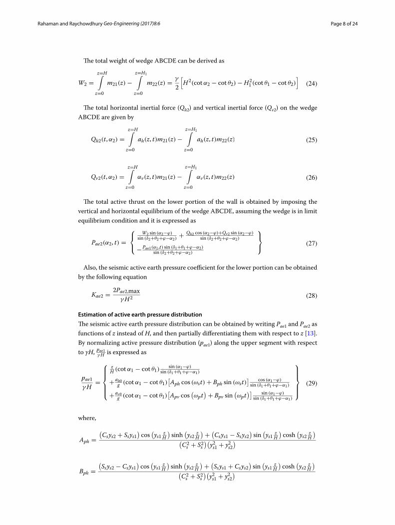
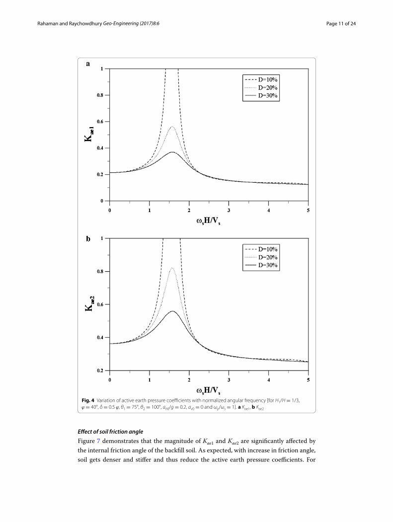
Figure  4 shows the variation of Kae1 and Kae2 with normalized angular frequency for different damping ratios assuming H1/H = 1/3, ϕ = 40◦, δ = 0.5 ϕ θ1 = 75◦, θ2 = 100◦ , ah0/g = 0.2 av0 = 0 and ωp/ωs = 1. It can be observed that the trend of the curve is not monotonic and there is a distinct increase for ωsH/Vs =  1.57. After a sharp increase, the curve decreases monotonically. These peaks correspond to the resonance, i.e., the frequency of the incident wave is close to the natural frequency of the backfill. It is also observed that the damping ratio has significant effect on the seismic active earth pres-sure coefficient near these amplification zones. The peak value of Kae1 and Kae2 decrease about 30 and 35%, respectively, for increase in damping ratio from 20 to 30%. Note that the effect of backfill damping is not significant beyond ωsH/Vs ≥ 2 and ωsH/Vs ≤ 0.5.

Effect of horizontal and vertical acceleration

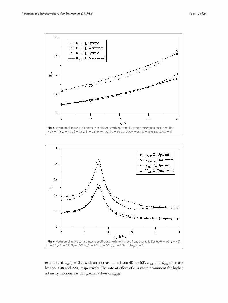
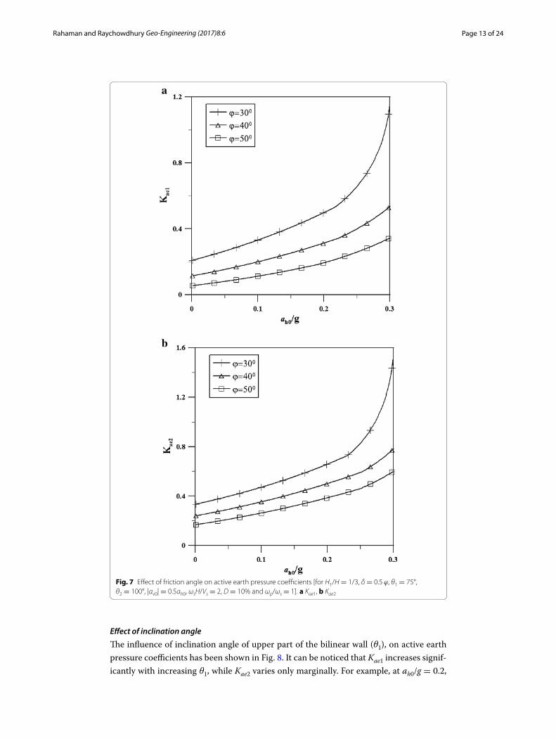
Figure 5 shows the variations of Kae1 and Kae2 with horizontal acceleration, ah0/g for two conditions: (1) Qv acting downward and (2) Qv acting upward. It is observed that the horizontal seismic acceleration coefficients for both the segments increase monotoni-cally as the horizontal inertia force on the backfill increases with increasing horizon-tal acceleration. It is obvious that the direction of acceleration during earthquake is not fixed; rather it changes its direction from cycle to cycle. This may subsequently cause a change in the direction of the seismic body forces with time. For evaluation of active earth pressure, the horizontal force must have to act towards the direction of wall face but the vertical force may act in upward or downward direction. Hence, there is always a phase difference between the horizontal seismic force and the vertical seismic force. The different directions of Qv imply that when the active thrust reaches its maximum for Qh, the Qv may either have a positive or a negative value. Hence, Kae1 and Kae2 may have different values for the same magnitude of Qv. The critical direction of the verti-cal force depends on many parameters, such as, soil friction angle, horizontal accelera-tion, non-dimensional frequency ratio and damping ratio of soil. It can be seen from Fig. 5 that for ωsH/Vs = 0.5, the critical condition for active thrust occurs when Qv acts downward for low intensity motions (low range of ah0/g). However, for high intensity motions, upward is more critical. This change in scenario happens at ah0/g = 0.3 for Kae1, and at ah0/g = 0.37 for Kae2. When plotted with normalized frequency ratio (Fig. 6), it is noted that the critical direction of vertical acceleration changes when the normalized frequency of the shear wave approaches the natural frequency of the backfill. Hence, it can be concluded from the above observations that the direction of vertical seismic force has significant effect on critical values of Kae1 and Kae2, and should be given required importance while estimating the seismic earth pressures.

Page 11 of 24Rahaman and Raychowdhury Geo-Engineering (2017) 8:6

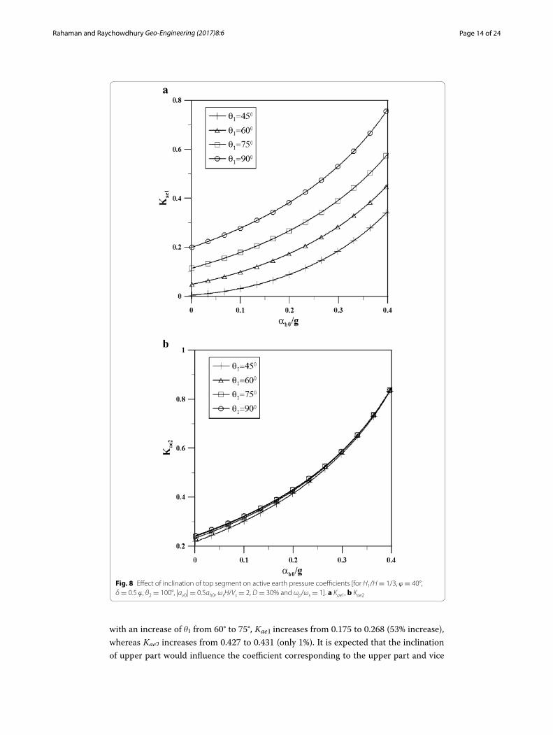
Effect of soil friction angle

Figure 7 demonstrates that the magnitude of Kae1 and Kae2 are significantly affected by the internal friction angle of the backfill soil. As expected, with increase in friction angle, soil gets denser and stiffer and thus reduce the active earth pressure coefficients. For

Fig. 4 Variation of active earth pressure coefficients with normalized angular frequency [for H1/H = 1/3, ϕ = 40°, δ = 0.5 ϕ, θ1 = 75°, θ2 = 100°, ah0/g = 0.2, av0 = 0 and ωp/ωs = 1]. a Kae1, b Kae2

Page 12 of 24Rahaman and Raychowdhury Geo-Engineering (2017) 8:6

example, at ah0/g =  0.2, with an increase in ϕ from 40° to 50°, Kae1 and Kae2 decrease by about 38 and 22%, respectively. The rate of effect of ϕ is more prominent for higher intensity motions, i.e., for greater values of ah0/g.

Fig. 6 Variation of active earth pressure coefficients with normalized frequency ratio [for H1/H = 1/3, ϕ = 40°, δ = 0.5 ϕ, θ1 = 75°, θ2 = 100°, ah0/g = 0.2, av0 = 0.5ah0, D = 20% and ωp/ωs = 1]

Fig. 5 Variation of active earth pressure coefficients with horizontal seismic acceleration coefficient [for H1/H = 1/3 ϕ, = 40°, δ = 0.5 ϕ, θ1 = 75°, θ2 = 100°, av0 = 0.5ah0, ωsH/Vs = 0.5, D = 10% and ωp/ωs = 1]

Page 13 of 24Rahaman and Raychowdhury Geo-Engineering (2017) 8:6

Effect of inclination angle

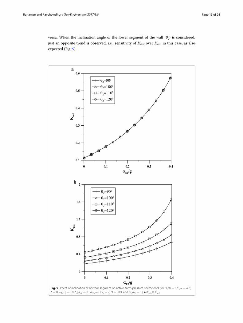
The influence of inclination angle of upper part of the bilinear wall (θ1), on active earth pressure coefficients has been shown in Fig. 8. It can be noticed that Kae1 increases signif-icantly with increasing θ1, while Kae2 varies only marginally. For example, at ah0/g = 0.2,

Fig. 7 Effect of friction angle on active earth pressure coefficients [for H1/H = 1/3, δ = 0.5 ϕ, θ1 = 75°, θ2 = 100°, |av0| = 0.5ah0, ωsH/Vs = 2, D = 10% and ωp/ωs = 1]. a Kae1, b Kae2

Page 14 of 24Rahaman and Raychowdhury Geo-Engineering (2017) 8:6

with an increase of θ1 from 60° to 75°, Kae1 increases from 0.175 to 0.268 (53% increase), whereas Kae2 increases from 0.427 to 0.431 (only 1%). It is expected that the inclination of upper part would influence the coefficient corresponding to the upper part and vice

Fig. 8 Effect of inclination of top segment on active earth pressure coefficients [for H1/H = 1/3, ϕ = 40°, δ = 0.5 ϕ, θ2 = 100°, |av0| = 0.5ah0, ωsH/Vs = 2, D = 30% and ωp/ωs = 1]. a Kae1, b Kae2

Page 15 of 24Rahaman and Raychowdhury Geo-Engineering (2017) 8:6

versa. When the inclination angle of the lower segment of the wall (θ2) is considered, just an opposite trend is observed, i.e., sensitivity of Kae2 over Kae1 in this case, as also expected (Fig. 9).

Fig. 9 Effect of inclination of bottom segment on active earth pressure coefficients [for H1/H = 1/3, ϕ = 40°, δ = 0.5 ϕ, θ2 = 100°, |av0| = 0.5ah0, ωsH/Vs = 2, D = 30% and ωp/ωs = 1]. a Kae1, b Kae2

Page 16 of 24Rahaman and Raychowdhury Geo-Engineering (2017) 8:6

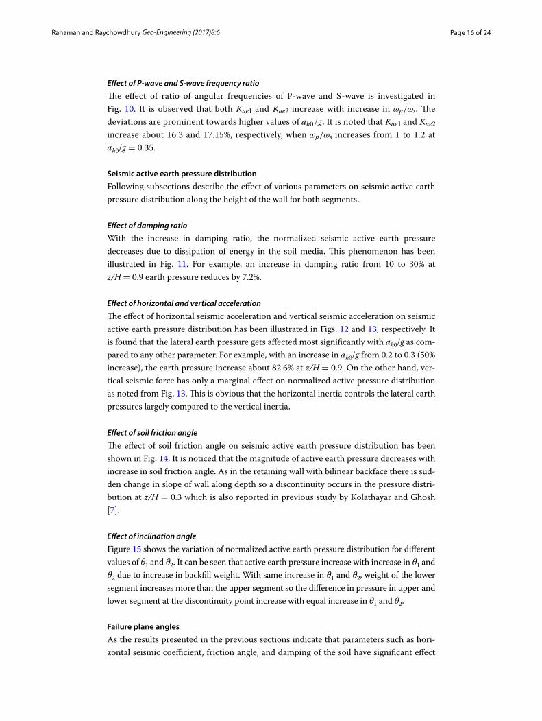
Effect of P‑wave and S‑wave frequency ratio

The effect of ratio of angular frequencies of P-wave and S-wave is investigated in Fig.  10. It is observed that both Kae1 and Kae2 increase with increase in ωp/ωs. The deviations are prominent towards higher values of ah0/g . It is noted that Kae1 and Kae2 increase about 16.3 and 17.15%, respectively, when ωp/ωs increases from 1 to 1.2 at ah0/g = 0.35.

Seismic active earth pressure distribution

Following subsections describe the effect of various parameters on seismic active earth pressure distribution along the height of the wall for both segments.

Effect of damping ratio

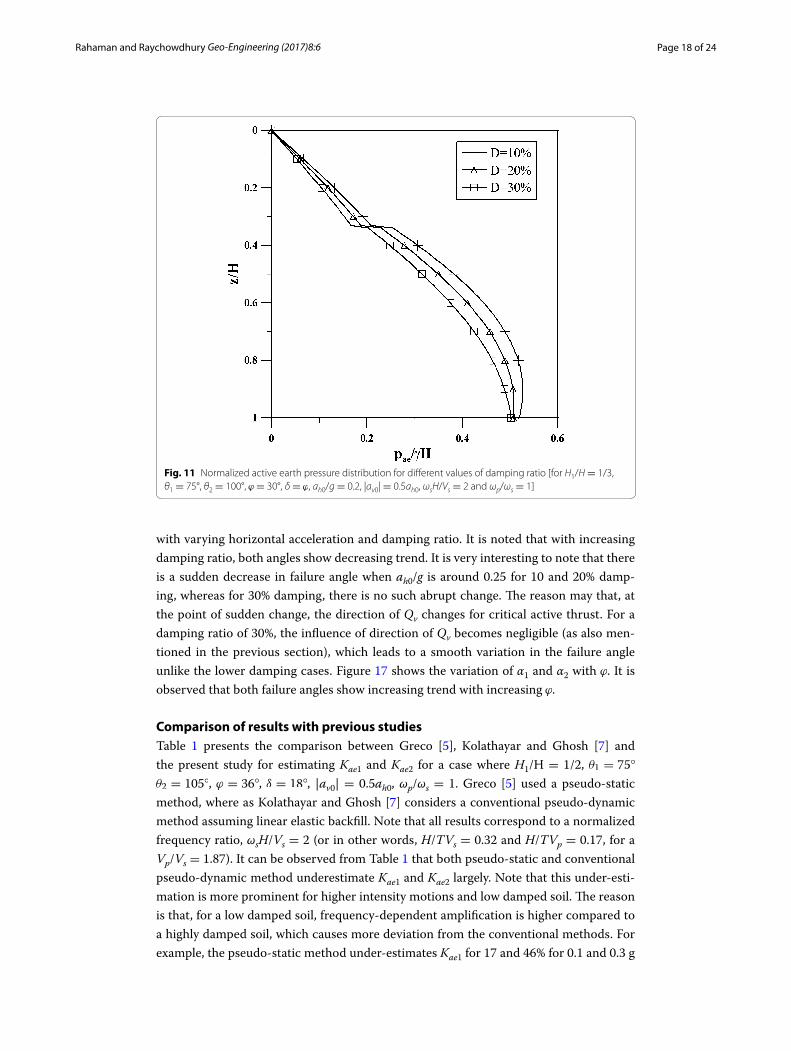
With the increase in damping ratio, the normalized seismic active earth pressure decreases due to dissipation of energy in the soil media. This phenomenon has been illustrated in Fig.  11. For example, an increase in damping ratio from 10 to 30% at z/H = 0.9 earth pressure reduces by 7.2%.

Effect of horizontal and vertical acceleration

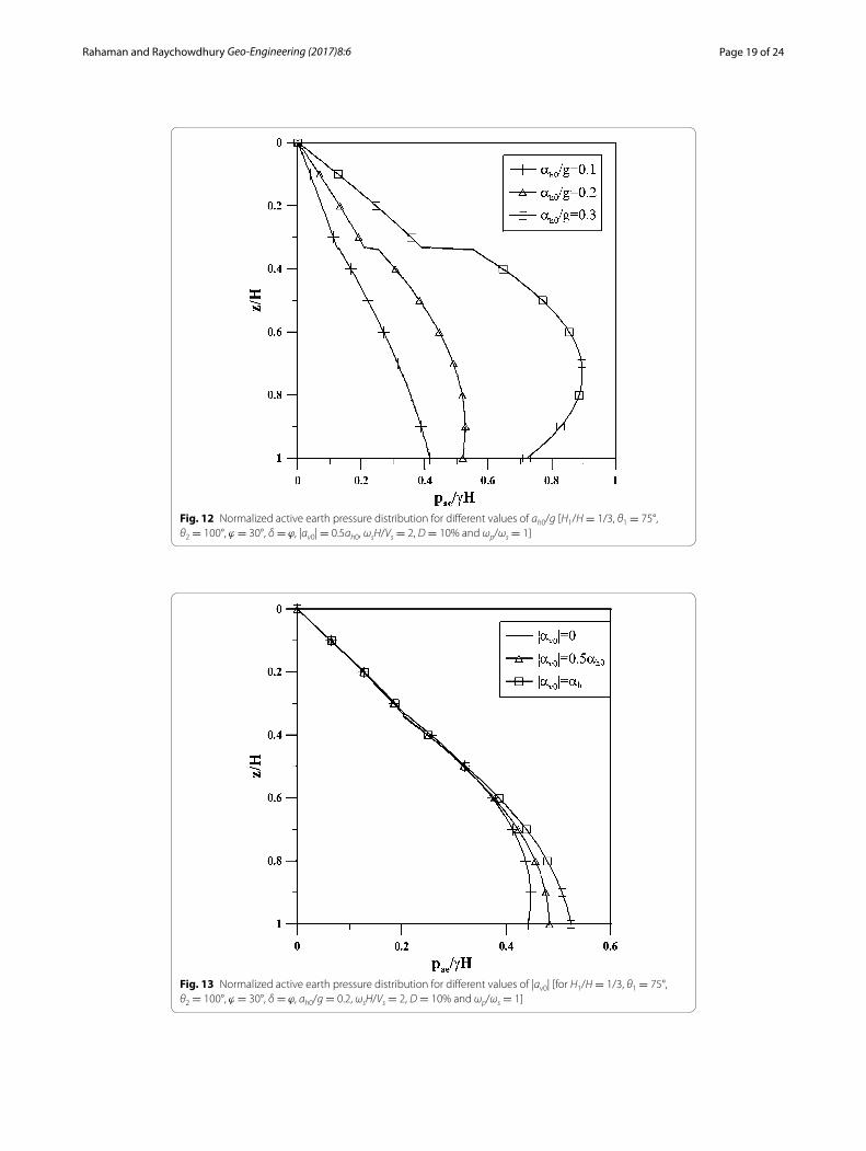
The effect of horizontal seismic acceleration and vertical seismic acceleration on seismic active earth pressure distribution has been illustrated in Figs. 12 and 13, respectively. It is found that the lateral earth pressure gets affected most significantly with ah0/g as com-pared to any other parameter. For example, with an increase in ah0/g from 0.2 to 0.3 (50% increase), the earth pressure increase about 82.6% at z/H = 0.9. On the other hand, ver-tical seismic force has only a marginal effect on normalized active pressure distribution as noted from Fig. 13. This is obvious that the horizontal inertia controls the lateral earth pressures largely compared to the vertical inertia.

Effect of soil friction angle

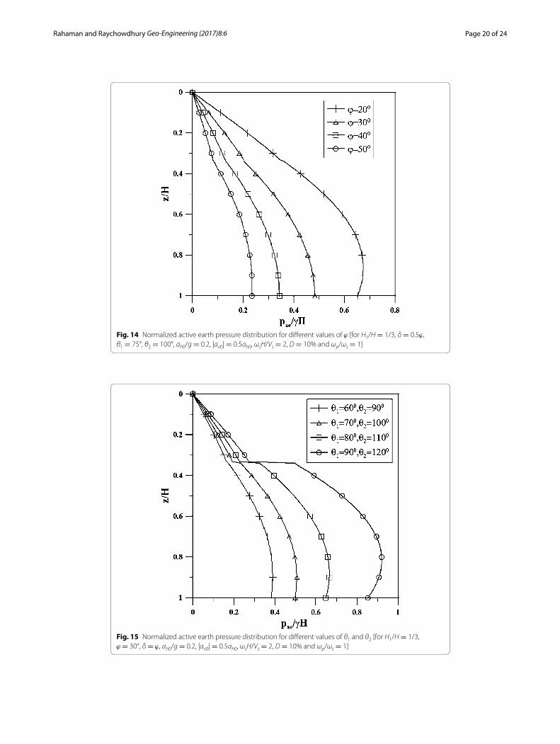
The effect of soil friction angle on seismic active earth pressure distribution has been shown in Fig. 14. It is noticed that the magnitude of active earth pressure decreases with increase in soil friction angle. As in the retaining wall with bilinear backface there is sud-den change in slope of wall along depth so a discontinuity occurs in the pressure distri-bution at z/H = 0.3 which is also reported in previous study by Kolathayar and Ghosh [7].

Effect of inclination angle

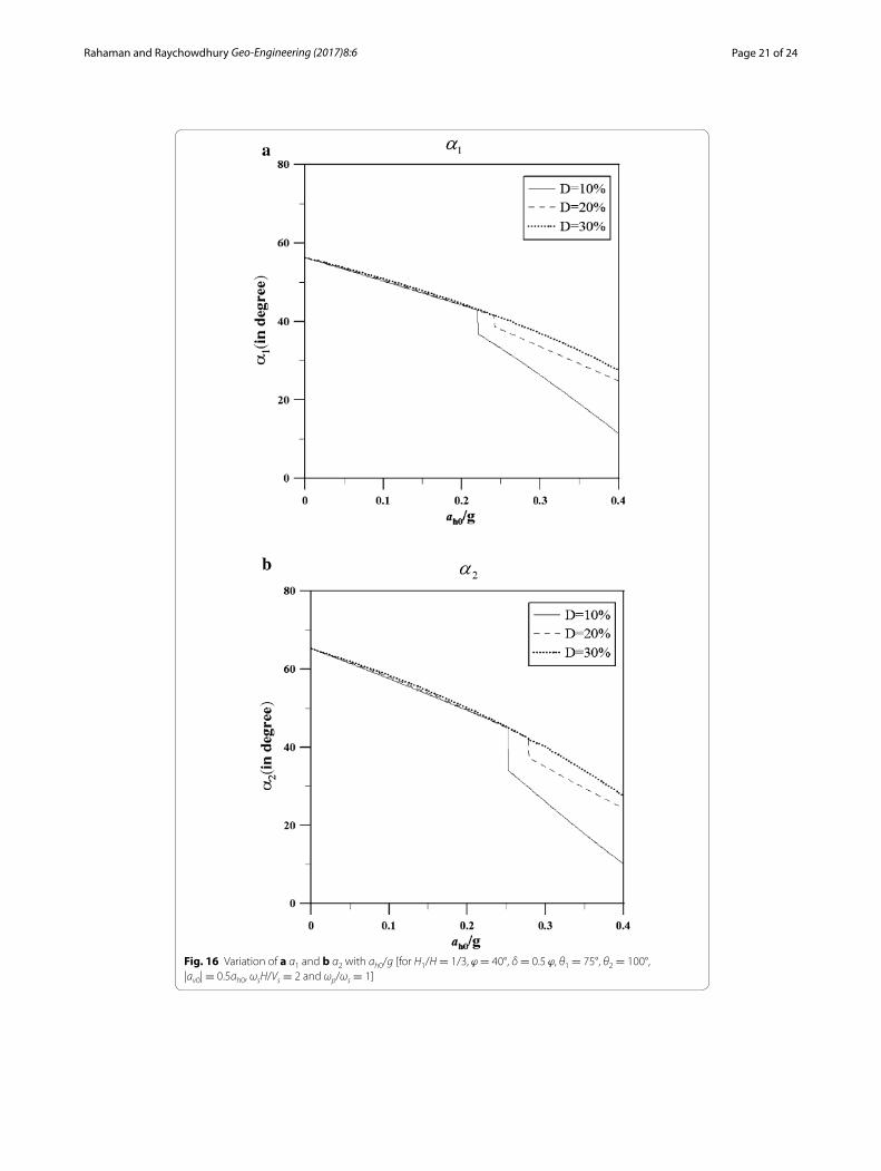
Figure 15 shows the variation of normalized active earth pressure distribution for different values of θ1 and θ2. It can be seen that active earth pressure increase with increase in θ1 and θ2 due to increase in backfill weight. With same increase in θ1 and θ2, weight of the lower segment increases more than the upper segment so the difference in pressure in upper and lower segment at the discontinuity point increase with equal increase in θ1 and θ2.

Failure plane angles

As the results presented in the previous sections indicate that parameters such as hori-zontal seismic coefficient, friction angle, and damping of the soil have significant effect

Page 17 of 24Rahaman and Raychowdhury Geo-Engineering (2017) 8:6

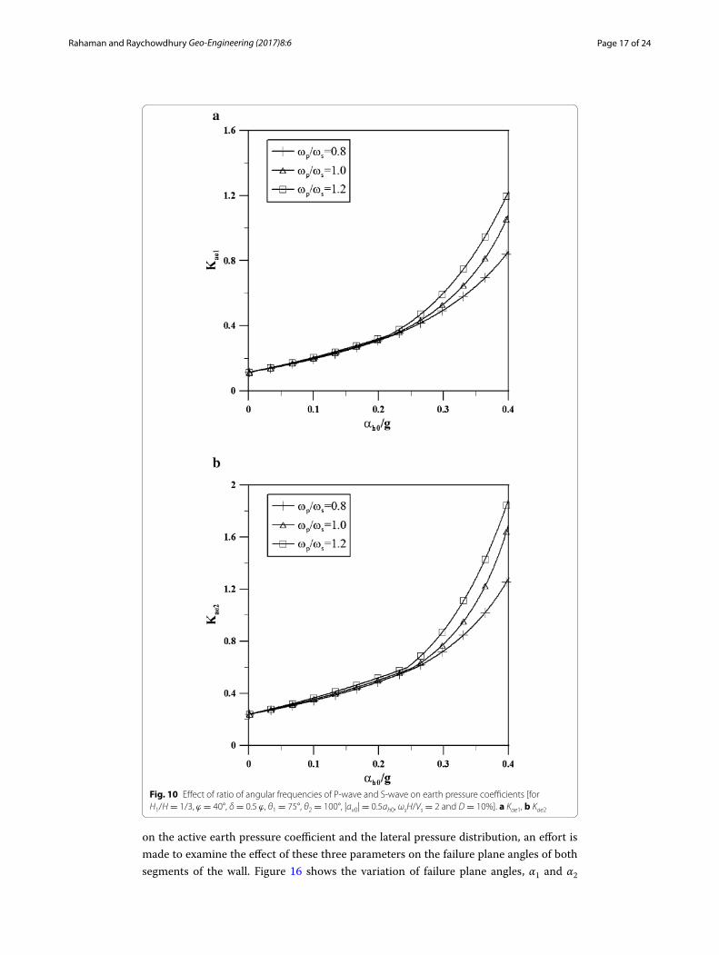
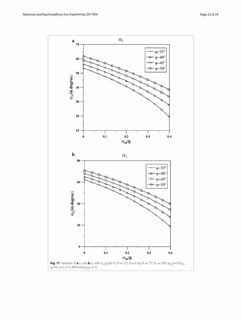
on the active earth pressure coefficient and the lateral pressure distribution, an effort is made to examine the effect of these three parameters on the failure plane angles of both segments of the wall. Figure  16 shows the variation of failure plane angles, α1 and α2

Fig. 10 Effect of ratio of angular frequencies of P-wave and S-wave on earth pressure coefficients [for H1/H = 1/3, ϕ = 40°, δ = 0.5 ϕ, θ1 = 75°, θ2 = 100°, |av0| = 0.5ah0, ωsH/Vs = 2 and D = 10%]. a Kae1, b Kae2

Page 18 of 24Rahaman and Raychowdhury Geo-Engineering (2017) 8:6

Fig. 11 Normalized active earth pressure distribution for different values of damping ratio [for H1/H = 1/3, θ1 = 75°, θ2 = 100°, ϕ = 30°, δ = ϕ, ah0/g = 0.2, |av0| = 0.5ah0, ωsH/Vs = 2 and ωp/ωs = 1]

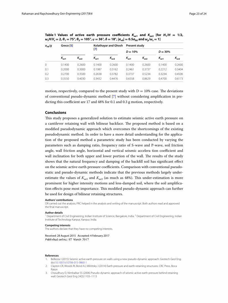
with varying horizontal acceleration and damping ratio. It is noted that with increasing damping ratio, both angles show decreasing trend. It is very interesting to note that there is a sudden decrease in failure angle when ah0/g is around 0.25 for 10 and 20% damp-ing, whereas for 30% damping, there is no such abrupt change. The reason may that, at the point of sudden change, the direction of Qv changes for critical active thrust. For a damping ratio of 30%, the influence of direction of Qv becomes negligible (as also men-tioned in the previous section), which leads to a smooth variation in the failure angle unlike the lower damping cases. Figure 17 shows the variation of α1 and α2 with ϕ. It is observed that both failure angles show increasing trend with increasing ϕ.

Comparison of results with previous studiesTable  1 presents the comparison between Greco [5], Kolathayar and Ghosh [7] and the present study for estimating Kae1 and Kae2 for a case where H1/H =  1/2, θ1 = 75◦ θ2 = 105◦, ϕ = 36◦, δ = 18◦, |av0| =  0.5ah0, ωp/ωs =  1. Greco [5] used a pseudo-static method, where as Kolathayar and Ghosh [7] considers a conventional pseudo-dynamic method assuming linear elastic backfill. Note that all results correspond to a normalized frequency ratio, ωsH/Vs = 2 (or in other words, H/TVs = 0.32 and H/TVp = 0.17, for a Vp/Vs = 1.87). It can be observed from Table 1 that both pseudo-static and conventional pseudo-dynamic method underestimate Kae1 and Kae2 largely. Note that this under-esti-mation is more prominent for higher intensity motions and low damped soil. The reason is that, for a low damped soil, frequency-dependent amplification is higher compared to a highly damped soil, which causes more deviation from the conventional methods. For example, the pseudo-static method under-estimates Kae1 for 17 and 46% for 0.1 and 0.3 g

Page 19 of 24Rahaman and Raychowdhury Geo-Engineering (2017) 8:6

Fig. 12 Normalized active earth pressure distribution for different values of ah0/g [H1/H = 1/3, θ1 = 75°, θ2 = 100°, ϕ = 30°, δ = ϕ, |av0| = 0.5ah0, ωsH/Vs = 2, D = 10% and ωp/ωs = 1]

Fig. 13 Normalized active earth pressure distribution for different values of |av0| [for H1/H = 1/3, θ1 = 75°, θ2 = 100°, ϕ = 30°, δ = ϕ, ah0/g = 0.2, ωsH/Vs = 2, D = 10% and ωp/ωs = 1]

Page 20 of 24Rahaman and Raychowdhury Geo-Engineering (2017) 8:6

Fig. 14 Normalized active earth pressure distribution for different values of ϕ [for H1/H = 1/3, δ = 0.5ϕ, θ1 = 75°, θ2 = 100°, ah0/g = 0.2, |av0| = 0.5ah0, ωsH/Vs = 2, D = 10% and ωp/ωs = 1]

Fig. 15 Normalized active earth pressure distribution for different values of θ1 and θ2 [for H1/H = 1/3, ϕ = 30°, δ = ϕ, ah0/g = 0.2, |av0| = 0.5ah0, ωsH/Vs = 2, D = 10% and ωp/ωs = 1]

Page 21 of 24Rahaman and Raychowdhury Geo-Engineering (2017) 8:6

Fig. 16 Variation of a α1 and b α2 with ah0/g [for H1/H = 1/3, ϕ = 40°, δ = 0.5 ϕ, θ1 = 75°, θ2 = 100°, |av0| = 0.5ah0, ωsH/Vs = 2 and ωp/ωs = 1]

Page 22 of 24Rahaman and Raychowdhury Geo-Engineering (2017) 8:6

Fig. 17 Variation of a α1 and b α2 with ah0/g [for H1/H = 1/3, δ = 0.5 ϕ, θ1 = 75°, θ2 = 100°, |av0| = 0.5ah0, ωsH/Vs = 2, D = 30% and ωp/ωs = 1]

Page 23 of 24Rahaman and Raychowdhury Geo-Engineering (2017) 8:6

motion, respectively, compared to the present study with D = 10% case. The deviations of conventional pseudo-dynamic method [7] without considering amplification in pre-dicting this coefficient are 17 and 48% for 0.1 and 0.3 g motion, respectively.

ConclusionsThis study proposes a generalized solution to estimate seismic active earth pressure on a cantilever retaining wall with bilinear backface. The proposed method is based on a modified pseudodynamic approach which overcomes the shortcomings of the existing pseudodynamic method. In order to have a more detail understanding for the applica-tion of the proposed method a parametric study has been conducted by varying the parameters such as damping ratio, frequency ratio of S-wave and P-wave, soil friction angle, wall friction angle, horizontal and vertical seismic accelera tion coefficient and wall inclination for both upper and lower portion of the wall. The results of the study shows that the natural frequency and damping of the backfill soil has significant effect on the seismic active earth pressure coefficients. Comparison with conventional pseudo-static and pseudo-dynamic methods indicate that the previous methods largely under-estimate the values of Kae1 and Kae2 (as much as 48%). This under-estimation is more prominent for higher intensity motions and less-damped soil, where the soil amplifica-tion effects pose most importance. This modified pseudo-dynamic approach can further be used for design of bilinear retaining structures.Authors’ contributionsOR carried out the analysis; PRC helped in the analysis and writing of the manuscript. Both authors read and approved the final manuscript.

Author details1 Department of Civil Engineering, Indian Institute of Science, Bangalore, India. 2 Department of Civil Engineering, Indian Institute of Technology Kanpur, Kanpur, India.

Competing interestsThe authors declare that they have no competing interests.

Received: 28 August 2015 Accepted: 4 February 2017

References 1. Bellezza I (2015) Seismic active earth pressure on walls using a new pseudo-dynamic approach. Geotech Geol Eng.

doi:10.1007/s10706-015-9860-1 2. Clayton CR, Woods RI, Bond AJ, Milititsky J (2014) Earth pressure and earth-retaining structures. CRC Press, Boca

Raton 3. Choudhury D, Nimbalkar SS (2006) Pseudo-dynamic approach of seismic active earth pressure behind retaining

wall. Geotech Geol Eng 24(5):1103–1113

Table 1 Values of  active earth pressure coefficients Kae1 and  Kae2 [for H1/H  =  1/2, ωsH/Vs = 2, θ1 = 75°, θ2 = 105°, ϕ = 36°, δ = 18°, |av0| = 0.5ah0 and ωp/ωs = 1]

ah0/g Greco [5] Kolathayar and Ghosh [7]

Present study

D = 10% D = 30%

Kae1 Kae2 Kae1 Kae2 Kae1 Kae2 Kae1 Kae2

0 0.1400 0.2600 0.1400 0.2600 0.1400 0.2600 0.1400 0.2600

0.1 0.2000 0.3000 0.1987 0.3162 0.2461 0.3737 0.2212 0.3404

0.2 0.2700 0.3500 0.2638 0.3782 0.3737 0.5234 0.3234 0.4506

0.3 0.3550 0.4030 0.3432 0.4476 0.6558 0.8629 0.4700 0.6173

Page 24 of 24Rahaman and Raychowdhury Geo-Engineering (2017) 8:6

4. Das BM (1993) Principles of soil dynamics. PWS-KENT Publishing Company, Boston 5. Greco VR (2007) Analytical earth thrust on walls with bilinear backface. Proc Inst Civil Eng Geotech Eng 160(1):23–29 6. Ishibashi I, Zhang X (1993) Unified dynamic shear moduli and damping ratios of sand and clay. Soils Found

33(1):182–191 7. Kolathayar S, Ghosh P (2009) Seismic active earth pressure on walls with bilinear backface using pseudo-dynamic

approach. Comput Geotech 36(7):1229–1236 8. Kramer SL (1996) Geotechnical earthquake engineering. Prentice Hall, New Jersey 9. Rahaman O (2015) Various aspects of seismic active pressure on retaining walls using pseudo-dynamic method.

M-Tech thesis, Indian Institute of Technology, Kanpur 10. Sadrekarimi A, Ghalandarzadeh A, Sadrekarimi J (2008) Static and dynamic behavior of hunchbacked gravity quay

walls. Soil Dyn Earthq Eng 28(2):99–117 11. Seed HB, Wong RT, Idriss IM, Tokimatsu K (1986) Moduli and damping factors for dynamic analyses of cohesionless

soils. J Geotech Eng ASCE 112(11):1016–1032 12. Sokolovskii VV (1960) Statics of soil media. Butterworths Scientific Publications, London 13. Steedman RS, Zeng X (1990) The influence of phase on the calculation of pseudo-static earth pressure on a retain-

ing wall. Geotechnique 40(1):103–112 14. Yuan C, Peng S, Zhang Z, Liu Z (2006) Seismic wavepropagation in Kelvin–Voigt homogeneous visco-elasticmedia.

Sci China Ser D Earth Sci 49(2):147–153