Model Averaging in Markov-Switching Models:Predicting National Recessions with Regional Data∗

Pierre Guerin† Danilo Leiva-Leon‡

December 22, 2014

Abstract

This paper estimates and forecasts U.S. business cycle turning points with state-level data. The probabilities of recession are obtained from univariate and multivari-ate regime-switching models based on a pairwise combination of national and state-level data. We use two classes of combination schemes to summarize the informationfrom these models: Bayesian Model Averaging and Dynamic Model Averaging. Inaddition, we suggest the use of combination schemes based on the past predictiveability of a given model to estimate regimes. Both simulation and empirical exercisesunderline the utility of such combination schemes. Moreover, our best specificationprovides timely updates of the U.S. business cycles, and compares favorably withcompeting models.

Keywords: Markov-switching, Nowcasting, Forecasting, Business Cycles, Forecastcombination.

JEL Classification Code: C53, E32, E37.

∗We would like to thank Massimiliano Marcellino for helpful comments and suggestions on a previousversion of this paper as well as Lutz Kilian, Michael Owyang, James Hamilton, Ana Galvao, Jeremy Piger,Robert Lavigne, Michael Ehrmann and seminar participants at the Applied Time Series EconometricsWorkshop held at the Federal Reserve Bank of St. Louis and the 2014 CFE conference in Pisa for helpfuldiscussions and comments. The views expressed in this paper are those of the authors. No responsibilityfor them should be attributed to the Bank of Canada.†Bank of Canada, e-mail: pguerin@bank-banque-canada.ca‡Bank of Canada, e-mail: leiv@bank-banque-canada.ca

1

Non-technical summary

Combining forecasts from different models is frequently perceived as a useful way tomitigate time instability in the forecasting performance of individual models, and therebyultimately improve the overall forecasting performance. Moreover, regime switching mod-els are widely used to model non-linear relations in macroeconomics and finance. A keyadvantage of regime switching models is their ability to estimate both discrete and con-tinuous outcomes. For example, one may not only be interested in forecasting the levelof GDP growth, but also evaluating whether an economy is heading into recession. It istherefore a natural question to study how to combine information from competing regimeswitching models in a forecasting environment.

A key contribution of this paper is to suggest new combination schemes in the contextof regime switching models, and compare them with existing weighting schemes. In detail,we consider both constant and time-varying weights when calculating the models’ weights(i.e., Bayesian model averaging and Dynamic model averaging, respectively). Rather thancalculating weights exclusively based on the likelihood that is designed to best fit the data,we suggest to use weights that rely on how well a model describes the underlying regimes.Moreover, another contribution of this paper is to present how to perform Dynamic modelaveraging when estimating regime switching models. One key conclusion of this paper is toshow that combination schemes based on the past performance to evaluate regimes performbest if one is interested in estimating and forecasting discrete outcomes.

In doing so, we first perform a Monte Carlo experiment that relies on simulated datato study in a controlled experiment the different combination schemes outlined in thispaper. Second, our empirical application concentrates on predicting national U.S. recessionswith state-level employment data using alternatively industrial production and employmentas a measure of national economic activity. We show that our preferred specificationsprovide timely updates of the U.S. business cycles. This holds true over an extendedevaluation sample for the forecasting exercise that permits to alleviate concerns aboutspurious forecasting results, and also over a sample that considers real-time data so as tomimic as closely as possible the information set available at the time the forecasts weremade. Overall, we trust that the methods outlined in this paper can be implemented to alarge class of applications in applied macroeconomics and finance.

2

1 Introduction

Assessing the current state of the economy represents a key input for policy makers andinvestors in their decision-making process. However, current economic conditions are typ-ically subject to substantial uncertainty owing to the publication delay of macroeconomicvariables and data revisions that become available long after the initial estimates have beenreleased. Likewise, detecting business cycle turning points in real-time proves to be verychallenging. As a result, economists have developed tools to provide early assessments ofbusiness cycle turning points. In particular, regime switching models have long been usedto date and predict turning points. An important aspect of this type of models is thatregime changes are endogenously estimated in a purely data driven way.

Since the seminal work of Hamilton (1989), a number of extensions to regime-switchingmodels have been proposed to estimate turning points for the U.S. economy. In this context,dynamic factor models subject to regime changes are one of the most successful approaches.Relevant contributions include Kim (1994), Kim and Yooa (1995) and Kim and Nelson(1998). Moreover, Chauvet (1998) finds that this type of models perform well to datebusiness cycle turning points in an out-of-sample experiment. Kholodilin and Yao (2005)use leading indicators in a dynamic factor model to predict turning points. Recent workshave focused on analyzing the performance of regime switching models to forecast turningpoints using real-time data (Chauvet and Hamilton (2006) and Chauvet and Piger (2008))and allowing for mixed frequency data (Camacho et al. (2012), Guerin and Marcellino(2013) and Camacho et al. (2014)).

Alternative approaches used to infer turning points rely on vector autoregressive (VAR)models with regime switching parameters. Relevant works include Hamilton and Perez-Quiros (1996) and Cakmakli et al. (2013) who use information on leading economic indexesto predict cycles for Gross National Product and Industrial Production, respectively. Nale-waik (2012) emphasizes the predictive content of gross domestic income (GDI) to forecastU.S. recessions in real-time. Finally, Hamilton (2011) provides a comprehensive survey ofthe literature on predicting turning points in real-time.

In a forecasting context, it is standard practise to rely on a combination of models to dealwith model uncertainty and parameter instability. In fact, as discussed in Timmermann(2006), forecast combinations have frequently been found to produce better forecasts onaverage than methods based on the ex ante best individual forecasting model. An approachincreasingly used in empirical studies is Bayesian Model Averaging (BMA), proposed byRaftery et al. (1998) and Hoeting et al. (1999) for linear models, which produces weightsfor each model that are constant over time.

Recently, Raftery et al. (2010) proposed a Dynamic Model Averaging (DMA) approach,where the models’ weights are allowed to evolve over time. DMA has been applied to avariety of contexts. In detail, to Time-Varying Parameter (TVP) regression models toforecast inflation (Koop and Korobilis (2012), Chan et al. (2012) and Belmonte and Koop(2014)), the European Carbon market (Koop and Tole (2013)), and major monthly USmacroeconomic variables using information from Google searches (Koop and Onorante(2013)). In a multivariate context, DMA has been applied to linear VAR models (Koop

3

(2014) and Koop and Onorante (2012)), large TVP-VAR models (Koop and Korobilis(2013)) to forecast inflation, real output and interest rates as well as factor models (Koopand Korobilis (2011)) to forecast growth and inflation in the U.K. An alternative approachfor model combination is provided in Elliott and Timmermann (2005) that suggests to useweights that can vary according to Markov chains. Geweke and Amisano (2011) insteadfocus on constructing optimal weights by considering linear pools where the objective is tomaximize the historical log of predictive score. Del Negro et al. (2013) provides a dynamicversion of the linear pools approach.

Despite the extensive literature on model averaging to formulate continuous forecasts,little has been done regarding the study of averaging schemes in the context of discreteforecasts. To the best of our knowledge, there are very few related works in this researcharea. For example, Billio et al. (2012) compare the performance of combination schemes forlinear and regime switching models, while Billio et al. (2013) propose a time-varying com-bination approach for multivariate predictive densities. Moreover, Berge (2013) comparesmodel selection schemes based on boosting algorithms with a Bayesian model averagingweighting scheme for predicting U.S. recessions based on logistic regressions using a set ofeconomic and financial indicators. He finds that the results are comparable across thesedifferent weighting schemes.

The purpose of this paper is to contribute to this literature by evaluating differentmodel averaging approaches for Markov-switching models to nowcast and forecast businesscycle turning points in real-time. Specifically, we compare the forecasting performance ofaveraging schemes based on constant weights (BMA) with those based on time-varyingweights (DMA), adapting the DMA approach of Raftery et al. (2010) to (univariate andmultivariate) Markov-switching models. Moreover, a key contribution of this paper is topropose another criterion to estimate the models’ weights, which relies on the ability of eachmodel to fit business cycle turning points. It therefore differs from the standard approachthat is only based on the likelihood associated with each model to determine the weights.

In a Monte Carlo experiment, we study the relevance of these different weightingschemes. We do find evidence in favor of weighting schemes based on past predictiveperformance to classify regimes in that such combination schemes yield lower quadraticprobability score (our evaluation metric to evaluate how well a model estimates regimes).This holds true for both BMA and DMA weighting schemes.

The empirical application concentrates on predicting U.S. national recessions usingstate-level data. In this context, it is natural to think of the best way to combine in-formation from the different U.S. states to predict a national aggregate. Another reasonfor focusing on this application is to contribute to the literature on the relationship be-tween regional and national macroeconomic developments. Owyang et al. (2005), Hamiltonand Owyang (2012) and Leiva-Leon (2014) use state-level data to study the synchroniza-tion of business cycles across U.S. states, finding that despite the significant heterogeneityin cyclical fluctuations, states have become more synchronized since the mid-90s. Also,Owyang et al. (2014) use state-level data to forecast U.S. recessions from probit models,showing that enlarging a set of preselected national variables with state-level data on em-ployment growth substantially improves nowcasts and short-term forecasts of the business

4

cycle phases. We follow Owyang et al. (2014) in that we also use state-level employmentdata to predict national U.S. recessions. However, we focus on regime switching modelsrather than probit models that include the NBER datation of business cycle regimes as adependent variable, the latter approach being problematic in a forecasting context giventhe substantial publication delay in the announcements of the NBER business cycle turningpoints.

The main results can be summarized as follows. First, we find that it is relevant totake into account the models’ ability to estimate regimes when calculating models’ weightsif one is interested in regime classification. Indeed, our combination schemes based onthe quadratic probability score typically outperform combination schemes based on thelikelihood only. This is especially true in an out-of-sample context. Second, the use ofregional data improves the forecasting performance of the models compared with modelsusing exclusively national data. Third, the best forecasting model in the out-of-sampleexercise outperforms the anxious index from the Survey of Professional Forecasters atshort-forecasting horizons, which emphasizes the relevance of our framework. In addition,in a purely real-time environment, we also find that our best specifications provide timelyestimates of the latest U.S. recession.

The paper is organized as follows. Section 2 describes the models we use, and Section3 the different combination schemes we implement, and present the changes we make tothe standard combination schemes. In Section 4, a small-sample Monte Carlo experimentis conducted to evaluate in a controlled experiment the combination schemes outlined inthe previous section. Section 5 introduces the data, and details the results. Section 6concludes.

2 Econometric Framework

2.1 Univariate model

We first consider a univariate regime-switching model defined as follows:

yt = µk0 + µk1Skt + βkxkt + vkt (1)

where yt is a U.S. national indicator (employment or industrial production), xkt is total(non-farm) employment data for state k, both in growth rates, and vkt is the regressionerror term (it is assumed to be normally distributed, that is, vkt ∼ N(0, σ2

k)). Skt is astandard Markov-chain defined by the following constant transition probability:

pkij = P (Skt+1 = j|Skt = i), (2)

M∑j=1

pkij = 1∀i, jε{1, ...,M} (3)

5

where M is the number of regimes.

Note that this specification differs from the baseline specification in Owyang et al. (2005)in that equation (1) mixes national data (i.e., yt) with state-level data (i.e, the xkt ’s). Incontrast, Owyang et al. (2005) estimate univariate regime-switching model on state-leveldata only to study the synchronization of economic activity across U.S. states. Moreover,Hamilton and Owyang (2012) examine the synchronization of U.S. states’ business cyclesusing a panel data model under the assumption that a small number of clusters can explainthe dynamics of U.S. states’ business cycles. It is also worth mentioning the work ofOwyang et al. (2014) that estimate a probit model to forecast U.S. recessions using alarge number of covariates, including both national and state-level data. These authorsthen use Bayesian model averaging to select the most relevant predictors for forecastingU.S. recessions. Finally, a common feature of these works is to strive for parsimoniousspecifications to study business cycle dynamics, which is even more relevant in a forecastingcontext. This is guiding our modeling choice in equation (1) to study the relevance of state-level data to predict U.S. recessions.

In addition, we also use as a benchmark model a univariate regime-switching modelwith no exogenous predictor defined as:

yt = µ0 + µ1St + ut (4)

where ut ∼ N(0, σ2)

2.2 Multivariate model

We then move on to consider a bivariate model where both the state-level data and thenational data are stacked in the vector of dependent variables:

zt = Γ(Syt , Skt ) + εkt (5)

where zt = (yt, xkt )′, and Γ(Syt , S

kt ) = (µy0 + µy1S

yt , µ

k0 + µk1(Skt ))′. yt is the U.S. national

indicator, and xkt is the total (non-farm) employment data for state k, both in growthrates. εkt is normally distributed, and Syt and Skt are two independent Markov chains.

A few additional comments are required. First, we use a different Markov-chain (Syt andSkt ) for each equation of the VAR, assuming that they are independently generated. Thisimplies that regime changes at the national and state-level do not necessarily coincide, afeature that allows for the presence of the jobless recovery phenomenon observed in theU.S. employment data. Second, we do not include autoregressive dynamics in the model,which is often found to be important for continuous forecasts of economic activity (e.g.,GDP growth), since we are interested in estimating business cycle turning points wheremodeling persistence in the data is likely to deteriorate the ability of the model to detectregime switches. In that respect, we follow for example Granger and Terasvirta (1999).

6

3 Combination schemes

In the empirical application, univariate and bivariate specifications each generate 50estimates for the probability of recession (i.e., one for each U.S. state). This information issummarized using two different classes of combination schemes: Bayesian model averagingand dynamic model averaging.

3.1 Bayesian model averaging

3.1.1 Likelihood approach

Suppose that we have K different models, Mk for k = 1, ..., K, which all seek to explainyt. The model Mk depends upon the regression parameters of the econometric specification(univariate or multivariate), collected in the vector Θk. Hence, the posterior distributionfor the parameters calculated from model Mk can be written as:

f(Θk|yt,Mk) =f(yt|Θk,Mk)f(Θk|Mk)

f(yt|Mk). (6)

Analogously, as suggested by Koop (2003), if one is interested in comparing differentmodels, we can use Bayes’ rule to derive a probability statement about what we do notknow (i.e., whether model Mk is appropriate or not to explain yt) conditional on what wedo know (i.e., the data, yt). This implies that the posterior model probability can be usedto assess the degree of support for model k:

f(Mk|yt) =f(yt|Mk)f(Mk)

f(yt), (7)

where f(yt) =∑K

j=1 f(yt|Mj)f(Mj), f(Mk) is the prior probability that model k is true andf(yt|Mk) is the marginal likelihood for model k. Following Newton and Raftery (1994), themarginal likelihood is calculated from the harmonic mean estimator, which is a simulation-consistent estimate that uses samples from the posterior density.1 The harmonic meanestimator of the marginal likelihood is:

f(yt|Mk) =

(1

N

N∑n=1

1

f(yt|M (n)k )

)−1

(8)

where f(yt|M (n)k ) is the posterior density available from simulation n, and N is the total

number of simulations. Initially, one could assume that all models are equally likely, that

1Note that alternative approaches could be used to calculate the marginal likelihood (see, e.g., Chib(1995) or Fruhwirth-Schnatter (2004)). However, these alternative methods are typically computationallydemanding in that they require a substantial increase in the number of simulations, which is not suitable inour empirical application, since we have to estimate many models in a recursive out-of-sample forecastingexperiment.

7

is f(Mk) = 1K

. Alternatively, one could use the employment share of each U.S. state to setthe prior probability for each model. In the case of equal prior probability for each model,the weights for model k are simply given as:

f(Mk|yt) =f(yt|Mk)∑Kj=1 f(yt|Mj)

(9)

3.1.2 Combined approach

Given that our models are designed to predict NBER recessions rather than predictingthe national activity indicator yt, an alternative weighting scheme could be implemented toreflect this objective. Indeed, we can rely on Bayes’ rule to derive a probability statementabout the most appropriate model Mk to explain the regimes St conditional on the dataand the estimated probability of being in a given regime derived from the Hamilton filterfor Markov-switching models, P (St|yt).2 Therefore, the posterior model probability can beexpressed as:

f(Mk|yt, St) =f(yt, St|Mk)f(Mk)

f(yt, St)(10)

=f(St|yt,Mk)f(yt|Mk)f(Mk)

f(St|yt)f(yt)(11)

where f(St|yt)P (yt) =∑K

j=1 f(St|yt,Mj)f(yt|Mj)f(Mj), f(Mk) is the prior probabilitythat model k is true, f(yt|Mk) is the marginal likelihood for model k, and f(St|yt,Mk)indicates the model’s ability to fit the business cycle regimes. We use the inverse QuadraticProbability Score (QPS) to evaluate f(St|yt,Mk), since the QPS is the most commonmeasure to evaluate discrete outcomes in the business cycle literature.3 The QPS associatedto model k is defined as follows:

QPSk =2

T

T∑t=1

(P (Skt = 0|ψt)−NBERt)2, (12)

where P (Skt = 0|ψt) is the probability of being in recession, given information up to t,ψt, and NBERt is a dummy variable that takes on a value of 1 if the U.S. economy is inrecession at time t according to the NBER business cycle dating committee and 0 otherwise.QPS is bounded between 0 and 2, and perfect predictions yield a QPS of 0. Hence, the lowerthe QPS, the better the ability of the model to fit the U.S. business cycle is. Accordingly,the posterior model probability for model k reads as:

f(Mk|yt, St) =f(yt|Mk)f(Mk)QPS

−1k∑K

j=1 f(yt|Mj)f(Mj)QPS−1j

. (13)

2For ease of exposition, here, we only present the case of one single Markov chain driving the changesin the parameters of the model. The derivations can be relatively easily extended to the case of multipleMarkov chains, but this would come at the cost of a much more demanding notation.

3Note that alternative criteria could be used to evaluate the models’ ability to classify regimes. Forexample, the logarithmic probability score or the area under the Receiver Operating Characteristics (see,e.g., Berge and Jorda (2011)) could be used. However, to streamline the paper we exclusively use the QPS,which is the most commonly used criteria to evaluate discrete outcomes.

8

One could use the U.S. employment share of each state as prior probability for each modelor equal prior weights. In the case of equal prior probability for each model, the posteriorprobability is:

f(Mk|yt, St) =ηk∑Kj=1 ηj

, (14)

where

ηk =f(yt|Mk)

QPSk. (15)

3.1.3 QPS approach

Notice that the posterior model probability in Equation (10) focuses on a joint fit ofdata, yt, and business cycle phases, St. However, since we are only interested in assessingthe ability of model Mk in explaining the business cycle phases, St, we avoid conditioningon yt and following the reasoning in Section 3.1.2, propose the following expression for theposterior probability model:

f(Mk|St) =f(St|Mk)f(Mk)∑Kj=1 f(St|Mj)f(Mj)

(16)

=f(Mk)QPS

−1k∑K

j=1 f(Mj)QPS−1j

. (17)

In the case of equal prior probability for each model, the posterior probability is givenby the normalized inverse QPS:

f(Mk|yt) =QPS−1

k∑Kj=1QPS

−1j

. (18)

3.2 Dynamic model averaging

3.2.1 Raftery’s approach

Dynamic model averaging originates from the work of Raftery et al. (2010), and has beenfirst implemented in econometrics by Koop and Korobilis (2012) and Koop and Korobilis(2013).

To compute weights that vary over time associated to model k, we only need the predic-tive density at time t of the corresponding model, fk(yt|ψt−1), and a coefficient referred toas the forgetting factor, α. Denote πt−1|t−1,k the predicted probability that model k is themost appropriate for forecasting at time t− 1 given information up to time t− 1. Rafteryet al. (2010) suggest that predictions of πt−1|t−1,k can be done as follows:

πt|t−1,k =παt−1|t−1,k∑Kj=1 π

αt−1|t−1,j

(19)

9

where 0 < α < 1 is set to a fixed value slightly less than one. The forgetting factorα is the coefficient that governs the amount of persistence in the models’ weights. Thehigher the α, the higher the weight attached to past predictive performance is. FollowingRaftery et al. (2010), we first set α = 0.99, which implies that forecasting performance fromtwo years ago receives about 78.5 per cent weight compared with last period’s forecastingperformance. We also report results with α = 0.95 so as to give lower weights to pastforecasting performance (in this case, information from two years ago receives about 29 percent weight compared with last period’s information).

Once yt is observed, πt|t−1,k, can be updated by using the predictive density, as follows:

πt|t,k =πt|t−1,kfk(yt|ψt−1)∑Kj=1 πt|t−1,jfj(yt|ψt−1)

(20)

The last two equations are repeated consecutively for each t, starting with equal weight foreach model at t = 1.

Dynamic model averaging differs from Bayesian model averaging in that no simulationis required to calculate the models’ weights, and the weights vary over time (t = {1, ..., T}).A detailed explanation about the algorithm used to calculate DMA weights in the contextof Markov-switching models is presented in Appendix B.

3.2.2 Combined approach

In line with Section 3.1.2, we also allow for the possibility that both, the marginallikelihood and the cumulative QPS, could inform about the model’s ability to predictbusiness cycle phases. Therefore, the updating equation reads as:

πt|t,k =πt|t−1,kηt|t−1,k∑Kj=1 πt|t−1,jηt|t−1,j

, (21)

where

ηt|t−1,k =fk(yt|ψt−1)

Qt|t,k, (22)

and Qt|t,k is the cumulative QPS at time t for model k defined as:

Qt|t,k =2

t(

t∑τ=1

P (Skτ = 0|ψτ )−NBERτ )2. (23)

The model prediction equation remains the same as in equation (19).

3.2.3 QPS approach

Again, since we are only interested in predicting business cycle phases instead of forecast-ing the national activity variable, we modify the Raftery et al. (2010) approach. Specifically,in line with Section 3.1.3, in the updating equation, we replace the marginal likelihood,which measures how well the model fits the data, with a measure of goodness-of-fit forbusiness cycle regimes. Hence, the updating equation reads as:

πt|t,k =πt|t−1,kQ

−1t|t,k∑K

j=1 πt|t−1,jQ−1t|t,j

. (24)

10

4 Simulation Study

We conduct a Monte Carlo experiment to study in a controlled set-up the validity of thedifferent model averaging schemes detailed in the previous section. In doing so, we choosea data generating process that closely mimics the empirical application of the paper, albeitfor computational reasons the sample size and the number of predictors are restricted.Equations (25) to (27) detail the data generating process. First, the dependent variable ytis generated according to the following equation:

yt = µy0 + µy1St + εyt , (25)

where εyt ∼ N(0, σ2y), and (µy0, µ

y1) = (−1, 2).

The xk,t’s variables are instead generated from the following equation:

xk,t = µk0 + µk1St + σkεkt , for k = {1, ..., K}. (26)

where εkt ∼ N(0, σ2k).

4

The intercepts for the xk,t’s variables are given by:

µkj = µyj + µyj εk,j, for j = {0, 1}. (27)

where εk,j ∼ U(−1, 1), so that the intercepts for the xt’s variables are closely related to theintercepts of the variable yt.

While the intercepts’ values µy0 and µy1 are kept constant, we use four different valuesfor the variance of the innovations (σ2 = {0.5, 1, 1.5, 2}). Moreover, St is a standardfirst-order Markov chain with two regimes and constant transition probabilities given by:(p00, p11)=(0.8, 0.9). In this way, the first regime is associated with a negative growth rateand it is less persistent than the second regime, a common feature of business cycle seriesthat typically exhibit different regimes’ duration. Finally, the series are generated withlength T = 200 and the number of xt variables is set to K = 20. The total number ofreplications is set to 1000. For each replication, the total number of simulations to estimatethe model’s parameters is 3000, discarding the first 1000 simulations to account for start-upeffects.

Table 1 reports, for the different model-averaging schemes and under the different sce-narios considered (i.e., BMA, DMA and an equal-weight scheme), the average in-sampleQPS obtained across the 1000 replications.5 For ease of computations, we also assume thata single Markov chain St drives the changes for both the yt and xt’s variables.6

4Note that the variance of the innovations is the same for both the yt and the xt’s (i.e., σx = σy) so asto avoid large differences in volatility across series.

5We only consider in-sample Monte-Carlo experiments owing to the too demanding computational taskthat would be required for a fully recursive out-of-sample exercise.

6This is not too detrimental since our primary objective is to estimate turning points at the nationalor aggregate level, hence we do not loose much in assuming a single Markov-chain driving the parameterchanges in the bivariate case.

11

The results show that, first, in both univariate and bivariate cases, the lowest QPS’are obtained when using the QPS-based model averaging scheme. This holds true for bothDMA and BMA in the univariate case, and the differences are the most noticeable in theBMA context. Second, in the context of DMA, the combined weighting scheme that relieson both the QPS and the marginal likelihood is a very close second best weighting scheme,which further emphasizes the value of the QPS to calculate models’ weights. Third, asthe volatility of the series increases (i.e., for higher values of σ), the differences in termsof QPS across the weighting schemes tend to soften. This is relatively intuitive in that,given the DGP’s we consider, as the volatility of the series increases, regimes shifts in theseries become less apparent, and it is therefore more difficult to make inference on theregimes, which translates into higher QPS, and lower value added resulting from weightingschemes based on QPS. Overall, this simulation exercise underlines the relevance of ourmodel-averaged scheme based on past predictive performance to classify the regimes (i.e.,QPS-based). The next section evaluates the relevance of this framework from an empiricalpoint of view, forecasting national U.S. recessions based on a set of regional indicators.

5 Empirical Results

5.1 Data

We use alternatively industrial production and employment data as a measure of na-tional economic activity. These two indicators are available on a monthly basis, and arefrequently considered as important measures of economic activity in the U.S. The state-level data we use are the employees on non-farm payrolls data series published at a monthlyfrequency for each U.S. state by the U.S. Bureau of Labor Statistics (note that state-leveldata are not available for monthly industrial production). These data are available on anot seasonally adjusted basis since at least January 1960 for all U.S. states. In contrast,data on a seasonally adjusted basis are available since January 1990, and real-time datavintages are only available since June 2007 from the “Alfred” real-time database of theFederal Reserve Bank of St. Louis.7 All data are taken as 100 times the change in the log-level of the series to obtain monthly percent changes. To facilitate inference on the regimes,and obtain a long enough evaluation sample to assess the accuracy of the forecasts, we usedata starting from 1960, and the data are appropriately seasonally adjusted. Hence, thefull estimation sample extends from February 1960 to April 2014.

5.2 In-sample results

The in-sample results are based on the data vintage from May 2014 with last obser-vation for April 2014. For brevity, we only report the results for each of the individual

7Data are available on http://alfred.stlouisfed.org/, and are typically available with a roughlythree-week delay for the state-level data, about a 1-week delay for national employment, and a 2-weekdelay for industrial production.

12

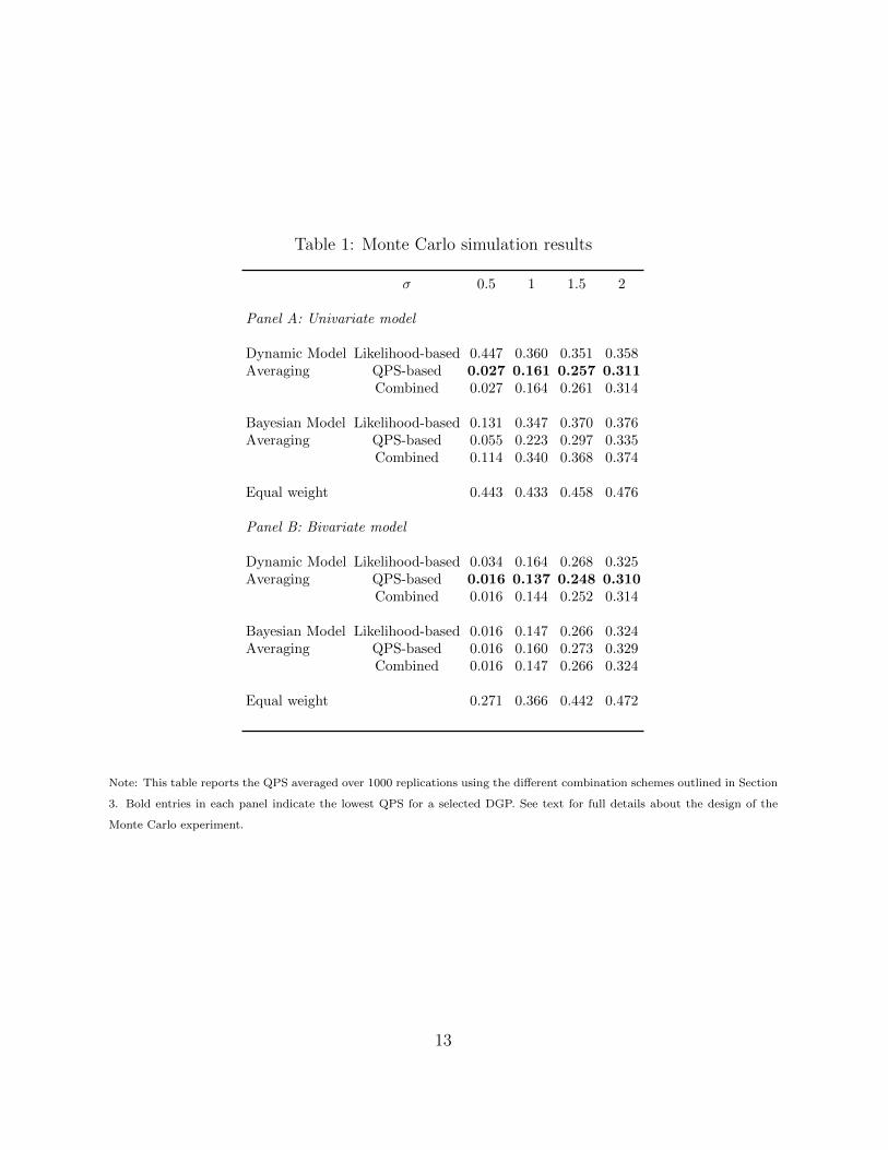
Table 1: Monte Carlo simulation results

σ 0.5 1 1.5 2

Panel A: Univariate model

Dynamic Model Likelihood-based 0.447 0.360 0.351 0.358Averaging QPS-based 0.027 0.161 0.257 0.311

Combined 0.027 0.164 0.261 0.314

Bayesian Model Likelihood-based 0.131 0.347 0.370 0.376Averaging QPS-based 0.055 0.223 0.297 0.335

Combined 0.114 0.340 0.368 0.374

Equal weight 0.443 0.433 0.458 0.476

Panel B: Bivariate model

Dynamic Model Likelihood-based 0.034 0.164 0.268 0.325Averaging QPS-based 0.016 0.137 0.248 0.310

Combined 0.016 0.144 0.252 0.314

Bayesian Model Likelihood-based 0.016 0.147 0.266 0.324Averaging QPS-based 0.016 0.160 0.273 0.329

Combined 0.016 0.147 0.266 0.324

Equal weight 0.271 0.366 0.442 0.472

Note: This table reports the QPS averaged over 1000 replications using the different combination schemes outlined in Section

3. Bold entries in each panel indicate the lowest QPS for a selected DGP. See text for full details about the design of the

Monte Carlo experiment.

13

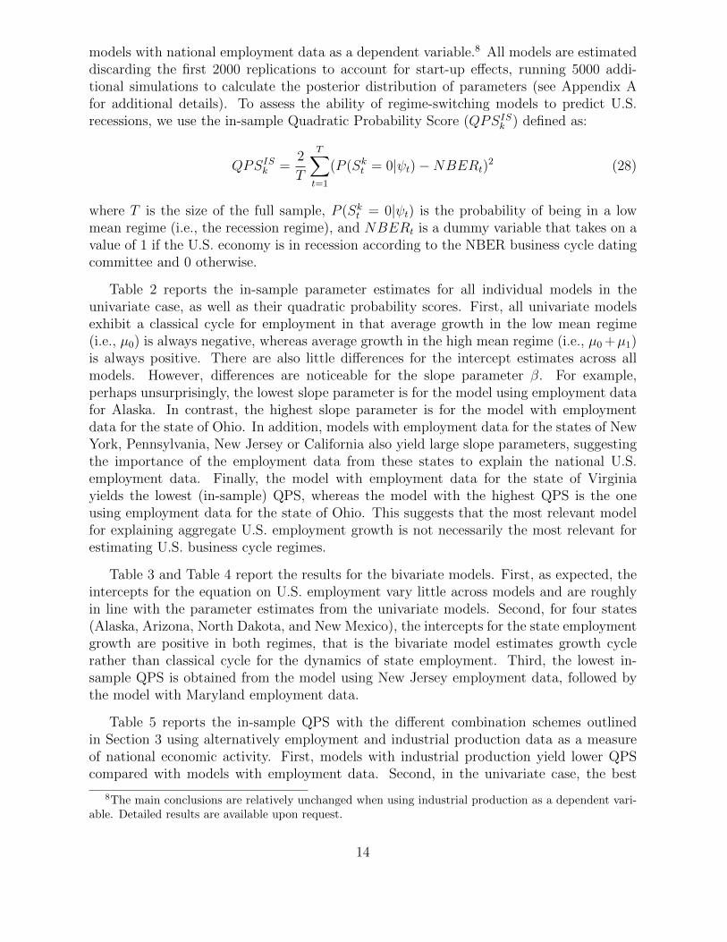
models with national employment data as a dependent variable.8 All models are estimateddiscarding the first 2000 replications to account for start-up effects, running 5000 addi-tional simulations to calculate the posterior distribution of parameters (see Appendix Afor additional details). To assess the ability of regime-switching models to predict U.S.recessions, we use the in-sample Quadratic Probability Score (QPSISk ) defined as:

QPSISk =2

T

T∑t=1

(P (Skt = 0|ψt)−NBERt)2 (28)

where T is the size of the full sample, P (Skt = 0|ψt) is the probability of being in a lowmean regime (i.e., the recession regime), and NBERt is a dummy variable that takes on avalue of 1 if the U.S. economy is in recession according to the NBER business cycle datingcommittee and 0 otherwise.

Table 2 reports the in-sample parameter estimates for all individual models in theunivariate case, as well as their quadratic probability scores. First, all univariate modelsexhibit a classical cycle for employment in that average growth in the low mean regime(i.e., µ0) is always negative, whereas average growth in the high mean regime (i.e., µ0 +µ1)is always positive. There are also little differences for the intercept estimates across allmodels. However, differences are noticeable for the slope parameter β. For example,perhaps unsurprisingly, the lowest slope parameter is for the model using employment datafor Alaska. In contrast, the highest slope parameter is for the model with employmentdata for the state of Ohio. In addition, models with employment data for the states of NewYork, Pennsylvania, New Jersey or California also yield large slope parameters, suggestingthe importance of the employment data from these states to explain the national U.S.employment data. Finally, the model with employment data for the state of Virginiayields the lowest (in-sample) QPS, whereas the model with the highest QPS is the oneusing employment data for the state of Ohio. This suggests that the most relevant modelfor explaining aggregate U.S. employment growth is not necessarily the most relevant forestimating U.S. business cycle regimes.

Table 3 and Table 4 report the results for the bivariate models. First, as expected, theintercepts for the equation on U.S. employment vary little across models and are roughlyin line with the parameter estimates from the univariate models. Second, for four states(Alaska, Arizona, North Dakota, and New Mexico), the intercepts for the state employmentgrowth are positive in both regimes, that is the bivariate model estimates growth cyclerather than classical cycle for the dynamics of state employment. Third, the lowest in-sample QPS is obtained from the model using New Jersey employment data, followed bythe model with Maryland employment data.

Table 5 reports the in-sample QPS with the different combination schemes outlinedin Section 3 using alternatively employment and industrial production data as a measureof national economic activity. First, models with industrial production yield lower QPScompared with models with employment data. Second, in the univariate case, the best

8The main conclusions are relatively unchanged when using industrial production as a dependent vari-able. Detailed results are available upon request.

14

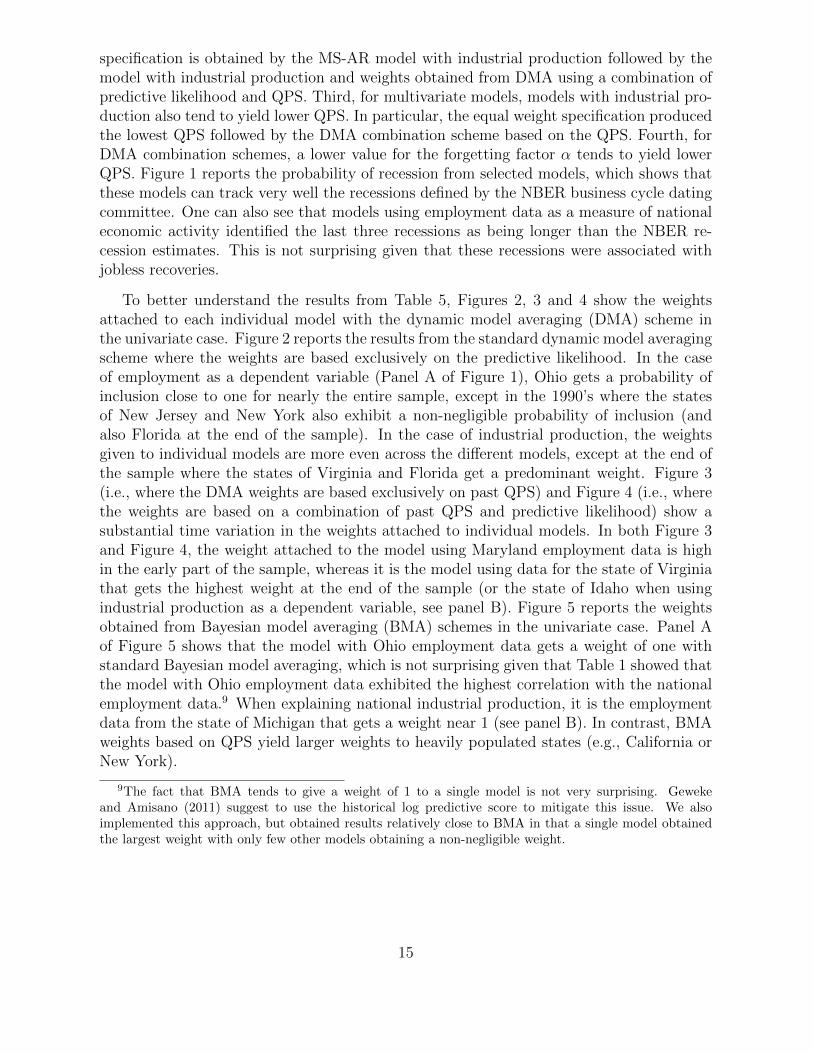
specification is obtained by the MS-AR model with industrial production followed by themodel with industrial production and weights obtained from DMA using a combination ofpredictive likelihood and QPS. Third, for multivariate models, models with industrial pro-duction also tend to yield lower QPS. In particular, the equal weight specification producedthe lowest QPS followed by the DMA combination scheme based on the QPS. Fourth, forDMA combination schemes, a lower value for the forgetting factor α tends to yield lowerQPS. Figure 1 reports the probability of recession from selected models, which shows thatthese models can track very well the recessions defined by the NBER business cycle datingcommittee. One can also see that models using employment data as a measure of nationaleconomic activity identified the last three recessions as being longer than the NBER re-cession estimates. This is not surprising given that these recessions were associated withjobless recoveries.

To better understand the results from Table 5, Figures 2, 3 and 4 show the weightsattached to each individual model with the dynamic model averaging (DMA) scheme inthe univariate case. Figure 2 reports the results from the standard dynamic model averagingscheme where the weights are based exclusively on the predictive likelihood. In the caseof employment as a dependent variable (Panel A of Figure 1), Ohio gets a probability ofinclusion close to one for nearly the entire sample, except in the 1990’s where the statesof New Jersey and New York also exhibit a non-negligible probability of inclusion (andalso Florida at the end of the sample). In the case of industrial production, the weightsgiven to individual models are more even across the different models, except at the end ofthe sample where the states of Virginia and Florida get a predominant weight. Figure 3(i.e., where the DMA weights are based exclusively on past QPS) and Figure 4 (i.e., wherethe weights are based on a combination of past QPS and predictive likelihood) show asubstantial time variation in the weights attached to individual models. In both Figure 3and Figure 4, the weight attached to the model using Maryland employment data is highin the early part of the sample, whereas it is the model using data for the state of Virginiathat gets the highest weight at the end of the sample (or the state of Idaho when usingindustrial production as a dependent variable, see panel B). Figure 5 reports the weightsobtained from Bayesian model averaging (BMA) schemes in the univariate case. Panel Aof Figure 5 shows that the model with Ohio employment data gets a weight of one withstandard Bayesian model averaging, which is not surprising given that Table 1 showed thatthe model with Ohio employment data exhibited the highest correlation with the nationalemployment data.9 When explaining national industrial production, it is the employmentdata from the state of Michigan that gets a weight near 1 (see panel B). In contrast, BMAweights based on QPS yield larger weights to heavily populated states (e.g., California orNew York).

9The fact that BMA tends to give a weight of 1 to a single model is not very surprising. Gewekeand Amisano (2011) suggest to use the historical log predictive score to mitigate this issue. We alsoimplemented this approach, but obtained results relatively close to BMA in that a single model obtainedthe largest weight with only few other models obtaining a non-negligible weight.

15

Table 2: In-sample parameter estimates - Univariate models

State µ0 µ1 β QPS µ0 µ1 β QPS

Alabama -0.099 0.266 0.263 0.191 Montana -0.149 0.352 0.082 0.179[-0.119,-0.079] [0.244,0.287] [0.241,0.285] [-0.170,-0.128] [0.330,0.374] [0.065,0.098]

Alaska -0.152 0.370 0.000 0.169 Nebraska -0.145 0.324 0.209 0.167[-0.175,-0.128] [0.346,0.393] [-0.011,0.010] [-0.168,-0.122] [0.300,0.347] [0.183,0.235]

Arizona -0.140 0.282 0.181 0.169 Nevada -0.152 0.325 0.090 0.160[-0.162,-0.117] [0.258,0.307] [0.174,0.201] [-0.175,-0.129] [0.301,0.350] [0.073,0.106]

Arkansas -0.138 0.310 0.193 0.190 New Hampshire -0.137 0.300 0.215 0.172[-0.158,-0.118] [0.290,0.332] [0.174,0.211] [-0.169,-0.112] [0.275,0.328] [0.193,0.238]

California -0.111 0.240 0.349 0.145 New Jersey -0.145 0.300 0.364 0.127[-0.135,-0.087] [0.213,0.266] [0.317,0.380] [-0.170,-0.124] [0.279,0.324] [0.339,0.388]

Colorado -0.177 0.324 0.223 0.124 New Mexico -0.141 0.322 0.166 0.179[-0.202,-0.150] [0.299,0.349] [0.199,0.248] [-0.164,-0.118] [0.297,0.345] [0.143,0.191]

Connecticut -0.124 0.306 0.222 0.126 New York -0.098 0.270 0.418 0.202[-0.157,-0.095] [0.276,0.335] [0.198,0.245] [-0.131,-0.071] [0.246,0.300] [0.383,0.452]

Delaware -0.137 0.339 0.073 0.171 North Carolina -0.115 0.243 0.325 0.154[-0.161,-0.113] [0.315,0.363] [0.061,0.085] [-0.139,-0.090] [0.218,0.267] [0.300,0.349]

Florida -0.124 0.243 0.290 0.215 North Dakota -0.149 0.353 0.071 0.176[-0.146,-0.103] [0.222,0.265] [0.267,0.313] [-0.171,-0.126] [0.330,0.376] [0.049,0.093]

Georgia -0.112 0.234 0.290 0.152 Ohio -0.023 0.168 0.452 0.247[-0.143,-0.087] [0.210,0.262] [0.295,0.341] [-0.042,-0.004] [0.150,0.187] [0.430,0.472]

Hawaii -0.150 0.352 0.078 0.165 Oklahoma -0.134 0.324 0.144 0.166[-0.173,-0.127] [0.329,0.375] [0.060,0.095] [-0.162,-0.109] [0.299,0.350] [0.122,0.168]

Idaho -0.145 0.335 0.100 0.179 Oregon -0.119 0.293 0.159 0.177[-0.166,-0.123] [0.313,0.357] [0.083,0.118] [-0.142,-0.095] [0.268,0.318] [0.136,0.182]

Illinois -0.064 0.238 0.335 0.200 Pennsylvania -0.072 0.246 0.384 0.218[-0.087,-0.043] [0.217,0.261] [0.309,0.360] [-0.092,-0.054] [0.227,0.267] [0.357,0.411]

Indiana -0.073 0.237 0.287 0.220 Rhode Island -0.113 0.307 0.172 0.177[-0.092,-0.055] [0.217,0.257] [0.269,0.306] [-0.137,-0.090] [0.284,0.330] [0.153,0.191]

Iowa -0.122 0.301 0.222 0.175 South Carolina -0.109 0.266 0.230 0.177[-0.142,-0.102] [0.280,0.322] [0.199,0.245] [-0.131,-0.087] [0.242,0.288] [0.209,0.252]

Kansas -0.130 0.325 0.123 0.172 South Dakota -0.150 0.344 0.123 0.179[-0.152,-0.108] [0.303,0.347] [0.105,0.141] [-0.171,-0.128] [0.323,0.366] [0.102,0.144]

Kentucky -0.129 0.306 0.184 0.166 Tennessee -0.109 0.261 0.274 0.198[-0.147,-0.109] [0.286,0.326] [0.168,0.200] [-0.131,-0.089] [0.241,0.283] [0.255,0.293]

Louisiana -0.138 0.342 0.087 0.180 Texas -0.124 0.257 0.315 0.187[-0.161,-0.115] [0.319,0.365] [0.069,0.104] [-0.152,-0.098] [0.232,0.284] [0.284,0.345]

Maine -0.129 0.317 0.164 0.165 Utah -0.143 0.316 0.148 0.167[-0.155,-0.104] [0.292,0.342] [0.141,0.186] [-0.167,-0.120] [0.291,0.340] [0.125,0.171]

Maryland -0.159 0.329 0.206 0.131 Vermont -0.135 0.323 0.134 0.172[-0.181,-0.136] [0.305,0.351] [0.184,0.227] [-0.158,-0.112] [0.299,0.346] [0.115,0.154]

Massachusetts -0.134 0.305 0.268 0.121 Virginia -0.171 0.301 0.309 0.097[-0.189,-0.087] [0.267,0.351] [0.234,0.298] [-0.207,-0.137] [0.272,0.330] [0.282,0.337]

Michigan -0.103 0.300 0.131 0.201 Washington -0.128 0.295 0.190 0.176[-0.121,-0.083] [0.279,0.319] [0.120,0.142] [-0.150,-0.108] [0.272,0.317] [0.166,0.215]

Minnesota -0.107 0.256 0.305 0.179 Wisconsin -0.112 0.278 0.258 0.183[-0.126,-0.088] [0.236,0.277] [0.280,0.329] [-0.133,-0.090] [0.255,0.301] [0.232,0.282]

Mississippi -0.121 0.288 0.223 0.185 West Virginia -0.142 0.358 0.035 0.176[-0.142,-0.100] [0.266,0.310] [0.204,0.242] [-0.165,-0.119] [0.335,0.381] [0.027,0.043]

Missouri -0.120 0.299 0.230 0.187 Wyoming -0.145 0.355 0.048 0.176[-0.138,-0.101] [0.280,0.319] [0.209,0.251] [-0.168,-0.122] [0.332,0.319] [0.034,0.061]

Note: µ0 is the mean growth rate in recession for aggregate U.S. employment, µ0 +µ1 is the mean growth rate in expansions for aggregate U.S.

employment, β is the parameter entering before the state-level employment data in equation (1). The parameter estimates are reported as the

median over 5000 replications. The estimation sample extends from February 1960 to April 2014. QPS is the Quadratic Probability Score for

individual models as defined in equation (28), and the 90 per cent coverage intervals are reported in brackets.

16

Table 3: In-sample Parameter estimates - Multivariate models

State µ0 µ1 QPS µ0 µ1 QPS

Alabama -0.097 0.306 0.192 Montana -0.134 0.349 0.178[-0.128,-0.059] [0.262,0.340] [-0.155,-0.112] [0.327,0.371]

-0.128 0.317 -1.870 2.040[-0.911,-0.042] [0.228,1.055] [-2.234,-1.541] [1.711,2.403]

Alaska -0.150 0.368 0.169 Nebraska -0.114 0.326 0.161[-0.173,-0.125] [0.344,0.392] [-0.143,-0.089] [0.301,0.354]

0.161 2.115 -0.838 0.995[0.125,0.197] [1.933,2.302] [-1.178,-0.017] [0.209,1.330]

Arizona -0.101 0.308 0.189 Nevada -0.134 0.349 0.178[-0.126,-0.077] [0.284,0.334] [-0.158,-0.111] [0.325,0.373]

0.133 0.403 -0.125 0.640[0.085,0.176] [0.356,0.449] [-0.261,-0.016] [0.543,0.756]

Arkansas -0.104 0.310 0.186 New Hampshire -0.131 0.340 0.182[-0.126,-0.082] [0.288,0.332] [-0.157,-0.103] [0.311,0.369]

-1.641 1.829 -0.227 0.479[-1.975,-1.214] [1.394,2.164] [-0.330,-0.142] [0.400,0.568]

California -0.118 0.326 0.181 New Jersey -0.096 0.289 0.129[-0.144,-0.090] [0.299,0.353] [-0.124,-0.070] [0.264,0.319]

-0.099 0.362 -0.795 0.908[-0.133,-0.066] [0.326,0.396] [-0.966,-0.296] [0.434,1.076]

Colorado -0.121 0.332 0.179 New Mexico -0.122 0.334 0.168[-0.145,-0.097] [0.309,0.356] [-0.146,-0.096] [0.310,0.359]

-0.056 0.374 0.096 0.232[-0.100,-0.015] [0.333,0.418] [0.018,0.140] [0.186,0.280]

Connecticut -0.125 0.337 0.169 New York -0.112 0.314 0.178[-0.153,-0.097] [0.309,0.365] [-0.147,-0.077] [0.281,0.347]

-0.184 0.341 -0.113 0.220[-0.239,-0.130] [0.286,0.397] [-0.163,-0.073] [0.180,0.268]

Delaware -0.127 0.341 0.167 North Carolina -0.136 0.341 0.185[-0.153,-0.102] [0.317,0.366] [-0.161,-0.110] [0.313,0.366]

-1.910 2.088 -0.231 0.484[-2.405,-1.485] [1.665,2.581] [-0.280,-0.179] [0.430,0.535]

Florida -0.087 0.304 0.238 North Dakota -0.133 0.352 0.182[-0.119,-0.060] [0.277,0.334] [-0.157,-0.110] [0.329,0.376]

-0.064 0.436 0.121 0.563[-0.111,-0.020] [0.390,0.483] [0.100,0.142] [0.481,0.640]

Georgia -0.117 0.322 0.203 Ohio 0.013 0.166 0.252[-0.142,-0.091] [0.295,0.348] [-0.008,0.034] [0.147,0.185]

-0.172 0.448 -1.473 1.552[-0.226,-0.119] [0.393,0.504] [-1.734,-1.203] [1.284,1.814]

Hawaii -0.135 0.351 0.163 Oklahoma -0.133 0.348 0.167[-0.159,-0.110] [0.327,0.375] [-0.160,-0.105] [0.321,0.373]

-2.015 2.209 -0.218 0.453[-2.521,-1.575] [1.770,2.709] [-0.273,-0.161] [0.397,0.510]

Idaho -0.143 0.359 0.171 Oregon -0.155 0.368 0.162[-0.165,-0.120] [0.335,0.382] [-0.181,-0.130] [0.343,0.394]

-0.316 0.598 -0.316 0.598[-0.465,-0.165] [0.481,0.753] [-0.386,-0.255] [0.536,0.666]

Note: This table reports results from the estimation of equation (5). µ0 is the mean growth rate in recession, µ0 + µ1 is the mean growth rate

in expansions. For each state, the first row indicates the results for employment at the national level, whereas the second row indicates results

for employment at the state-level. The parameter estimates are reported as the median over 5000 replications. The estimation sample extends

from February 1960 to April 2014. QPS is the Quadratic Probability Score for individual models as defined in equation (28), and 90 per cent

coverage intervals are reported in brackets.

17

Table 4: In-sample Parameter estimates - Multivariate models (cont’d)

State µ0 µ1 QPS µ0 µ1 QPS

Illinois -0.106 0.317 0.196 Pennsylvania -0.095 0.301 0.191[-0.132,-0.081] [0.291,0.344] [-0.125,-0.066] [0.269,0.332]

-0.156 0.304 -0.156 0.263[-0.196,-0.116] [0.263,0.346] [-0.237,-0.106] [0.212,0.328]

Indiana -0.050 0.249 0.206 Rhode Island -0.108 0.315 0.175[-0.078,-0.027] [0.226,0.278] [-0.131,-0.084] [0.291,0.339]

-0.508 0.640 -1.101 1.199[-0.755,-0.342] [0.485,0.880] [-1.509,-0.836] [0.941,1.601]

Iowa -0.086 0.289 0.166 South Carolina -0.136 0.348 0.183[-0.108,-0.064] [0.268,0.311] [-0.159,-0.113] [0.323,0.371]

-1.353 1.494 -0.237 0.499[-1.539,-1.184] [1.322,1.679] [-0.318,-0.175] [0.434,0.576]

Kansas -0.108 0.318 0.166 South Dakota -0.135 0.352 0.178[-0.132,-0.084] [0.295,0.342] [-0.159,-0.112] [0.328,0.375]

-3.517 3.661 -0.017 0.248[-3.976,-3.045] [3.191,4.119] [-0.125,0.066] [0.175,0.341]

Kentucky -0.088 0.292 0.162 Tennessee -0.108 0.317 0.166[-0.108,-0.067] [0.271,0.313] [-0.133,-0.084] [0.291,0.344]

-1.178 1.359 -0.105 0.334[-1.438,-0.969] [1.153,1.615] [-0.164,-0.048] [0.274,0.394]

Louisiana -0.117 0.332 0.180 Texas -0.112 0.329 0.201[-0.142,-0.093] [0.309,0.356] [-0.138,-0.086] [0.304,0.354]

-4.004 4.157 -0.050 0.365[-4.342,-3.664] [3.816,4.495] [-0.086,-0.014] [0.330,0.401]

Maine -0.108 0.316 0.163 Utah -0.139 0.353 0.167[-0.135,-0.082] [0.291,0.342] [-0.163,-0.114] [0.328,0.377]

-2.373 2.498 -0.127 0.459[-2.787,-1.934] [2.057,2.913] [-0.189,-0.068] [0.404,0.517]

Maryland -0.126 0.330 0.137 Vermont -0.111 0.320 0.174[-0.150,-0.102] [0.307,0.356] [-0.134,-0.086] [0.296,0.385]

-0.959 1.135 -1.623 1.791[-1.278,-0.191] [0.387,1.452] [-2.087,-1.178] [1.344,2.253]

Massachusetts -0.107 0.319 0.194 Virginia -0.119 0.330 0.184[-0.135,-0.080] [0.293,0.347] [-0.144,-0.094] [0.303,0.356]

-0.264 0.410 -0.039 0.295[-0.317,-0.213] [0.359,0.463] [-0.098,0.017] [0.240,0.350]

Michigan -0.086 0.292 0.197 Washington -0.132 0.345 0.167[-0.107,-0.065] [0.270,0.313] [-0.157,-0.108] [0.321,0.369]

-3.291 3.403 -0.112 0.412[-3.666,-2.895] [3.007,3.773] [-0.162,-0.064] [0.364,0.461]

Minnesota -0.114 0.324 0.186 Wisconsin -0.133 0.345 0.186[-0.138,-0.088] [0.300,0.350] [-0.158,-0.109] [0.320,0.371]

-0.096 0.325 -0.178 0.371[-0.140,-0.053] [0.280,0.371] [-0.230,-0.127] [0.318,0.425]

Mississippi -0.077 0.313 0.188 West Virginia -0.133 0.351 0.177[-0.136,-0.077] [0.279,0.345] [-0.158,-0.109] [0.320,0.371]

-0.068 0.304 -6.175 6.286[-1.692,0.044] [0.225,1.856] [-6.708,-5.640] [5.748,6.815]

Missouri -0.095 0.299 0.178 Wyoming -0.143 0.360 0.171[-0.116,-0.074] [0.277,0.321] [-0.167,-0.117] [0.336,0.385]

-1.038 1.160 -0.751 0.981[-1.347,-0.866] [0.991,1.466] [-0.958,0.574] [0.811,1.183]

Note: See Table 3.

18

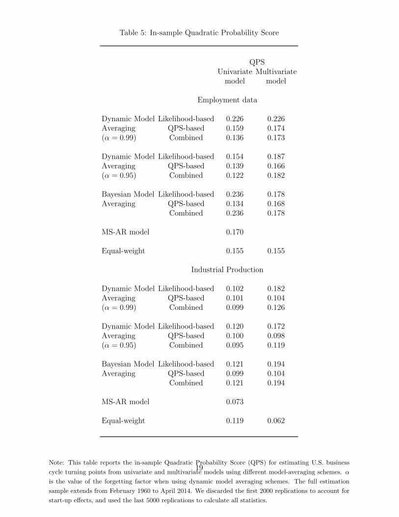
Table 5: In-sample Quadratic Probability Score

QPSUnivariate Multivariate

model model

Employment data

Dynamic Model Likelihood-based 0.226 0.226Averaging QPS-based 0.159 0.174(α = 0.99) Combined 0.136 0.173

Dynamic Model Likelihood-based 0.154 0.187Averaging QPS-based 0.139 0.166(α = 0.95) Combined 0.122 0.182

Bayesian Model Likelihood-based 0.236 0.178Averaging QPS-based 0.134 0.168

Combined 0.236 0.178

MS-AR model 0.170

Equal-weight 0.155 0.155

Industrial Production

Dynamic Model Likelihood-based 0.102 0.182Averaging QPS-based 0.101 0.104(α = 0.99) Combined 0.099 0.126

Dynamic Model Likelihood-based 0.120 0.172Averaging QPS-based 0.100 0.098(α = 0.95) Combined 0.095 0.119

Bayesian Model Likelihood-based 0.121 0.194Averaging QPS-based 0.099 0.104

Combined 0.121 0.194

MS-AR model 0.073

Equal-weight 0.119 0.062

Note: This table reports the in-sample Quadratic Probability Score (QPS) for estimating U.S. business

cycle turning points from univariate and multivariate models using different model-averaging schemes. α

is the value of the forgetting factor when using dynamic model averaging schemes. The full estimation

sample extends from February 1960 to April 2014. We discarded the first 2000 replications to account for

start-up effects, and used the last 5000 replications to calculate all statistics.

19

5.3 Out-of-sample results

5.3.1 Full evaluation sample

The first estimation sample extends from February 1960 to December 1978, and it isrecursively expanded until September 2013, that is the evaluation sample covers the periodranging from January 1979 to March 2014 (i.e., the last forecast six-month ahead refers tothe month of March 2014). As such, our evaluation sample includes five recessions thatcovers 13.2 per cent of the sample. Such a long evaluation permits to mitigate the risks ofspurious forecasting results. The models are re-estimated every month as new informationbecomes available.

We formulate forecasts for horizon h = {0, 1, 2, 3, 6}, that is from the current month(h = 0) up to six-month ahead (h = 6). We use the quadratic probability score (QPS) toevaluate the accuracy in predicting turning points. The out-of-sample QPS (QPSOOS) isdefined as follows:

QPSOOSk =2

T − T0 + 1

T∑t=T0

(P (Skt+h = 0|ψt)−NBERt+h)2 (29)

where T − T0 + 1 is the size of the evaluation sample, P (Skt+h = 0|ψt) is the probabilityof being in the first regime (i.e., the recession regime) in period t + h, and NBERt+h isa dummy variable that takes on a value of 1 if the U.S. economy is in recession in periodt+ h and 0 otherwise.

In comparing models, we also report results obtained from using the anxious index fromthe Survey of Professional Forecasters (SPF) of the Philadelphia Federal Reserve Bank.This index corresponds to the probability of a decline in real GDP. This is a relevantbenchmark, since survey forecasts have been found to perform very well compared withmodel-based predictions (see, e.g., Faust and Wright (2009)). The SPF is only availableon a quarterly basis, but we disaggregate it at the monthly frequency assuming that itsmonthly value is constant over the three months of the quarter. Moreover, we also evaluatethe statistical significance of our results using the Diebold-Mariano-West test to test forequal out-of-sample predictive accuracy (see Diebold and Mariano (1995) and West (1996)),using the likelihood-based weighting scheme as a benchmark model. In this way, we canevaluate from a statistical point of view the relevance of our weighting scheme based onthe QPS compared with the traditional approach that relies exclusively on the likelihood.

Table 6 reports the results for the univariate models and Table 7 displays the resultsfor the multivariate models. First, for univariate models, the combination scheme withindustrial production using DMA weights based on the QPS obtains the best forecastingresults for forecast horizons h = {0, 1, 2}, and the SPF anxious index obtained the bestresults for forecast horizons h = {3, 6}. Second, for multivariate models, the best resultsare obtained by the model using industrial production and DMA weights based on theQPS for forecast horizons h = {0, 1, 2}, and a combination of the predictive likelihood andQPS for forecast horizons h = {3, 6}. Third, the QPS-based combination schemes nearly

20

always outperforms the combination schemes based on the likelihood only, and typically ina statistically significant way.

Figure 6 reports the one-month-ahead predicted probability of being in a recession fromselected specifications. It shows that QPS-based DMA combination schemes perform wellin that they capture very well all U.S. recessions. However, an important caveat of theout-of-sample analysis so far is that we only used revised data. In the next sub-section, wemove to a real-time forecasting setting, concentrating on the prediction of the 2008-2009recession.10

5.3.2 A closer look at the Great Recession

Revisions to macroeconomic data are substantial (see e.g. Croushore and Stark (2001)).Using data as available at the time the forecasts are made is therefore critical to evaluaterealistically the models’ forecasting ability. Real-time employment data are available for all50 states starting from the June 2007 vintage with last observation for May 2007. Hence,our first estimation sample extends from February 1960 to May 2007, and it is recursivelyexpanded until August 2013. As a result, the evaluation sample extends from May 2007to August 2013, that is 76 months. In this case, since our evaluation sample only coversa limited period of time and only one recession, we do not calculate QPS statistics, butinstead report the probability of being in a recession - defined as the last estimate availablefor the average probability of being in a recession (i.e., P (St = 0|ψt) where t is the lastobservation in the estimation sample) - and compare it with a number of alternatives.

Figure 7 reports the results for selected specifications using the QPS-based weightingscheme along with the probability of recession derived from the SPF Anxious index. Indetail, this figure shows that the model using the employment data as a measure of nationaleconomic activity provides a timely update of the beginning of the recession in that theprobability of recession is above 0.5 as early as April 2008. However, this model detectsonly with a substantial lag the end of the recession owing to the very slow recovery inlabor market conditions. In contrast, the model using industrial production as a measureof national economic activity provides an accurate signal for the end of recession, butprovides a late call for the beginning of the recession. Interestingly, the performance ofthe SPF anxious index is somewhat inferior to these two models despite the fact that theSPF uses a much larger information set than our model-based estimates. In particular, theanxious index provides a call of recession later than the model using national employmentdata and detects the end of the recession later than the model using national industrialproduction data. Overall, this suggests that employment data are very helpful to detectthe beginning of recessions, whereas industrial production data rather provide valuableinformation about the end of recessions.

10As a robustness check, we also calculated QPS exclusively over the recession periods identified by theNBER (the results are not reported for space constraints). Over this restricted sample, the most accuratepredictions at short-forecasting horizons are obtained by models using national employment and combininginformation with DMA based on the QPS. As such, this broadly confirms the full sample estimates in thatweighting schemes based on the QPS provide valuable information.

21

Table 6: Out-of-sample Quadratic Probability Score - Univariate models

Employment

Forecast horizon (months) 0 1 2 3 6

Dynamic Model Likelihood-based 0.315 0.307 0.302 0.300 0.292Averaging QPS-based 0.184*** 0.197*** 0.214*** 0.227*** 0.252**α = 0.99 Combined 0.192*** 0.207*** 0.222*** 0.233*** 0.251**

Dynamic Model Likelihood-based 0.222 0.236 0.246 0.252 0.259Averaging QPS-based 0.176 0.193* 0.210* 0.223 0.247α = 0.95 Combined 0.185*** 0.206*** 0.222** 0.231** 0.248

Bayesian Model Likelihood-based 0.374 0.359 0.348 0.340 0.321Averaging QPS-based 0.196*** 0.213*** 0.229*** 0.240*** 0.256***

Combined 0.374 0.359 0.348 0.340 0.321

Equal weight 0.209*** 0.223*** 0.237*** 0.248*** 0.263***

Industrial Production

Dynamic Model Likelihood-based 0.239 0.240 0.243 0.248 0.252Averaging QPS-based 0.108*** 0.136*** 0.165** 0.188** 0.227α = 0.99 Combined 0.108*** 0.135*** 0.165** 0.187** 0.227

Dynamic Model Likelihood-based 0.216 0.221 0.228 0.235 0.243Averaging QPS-based 0.101*** 0.133*** 0.164** 0.187* 0.227α = 0.95 Combined 0.110*** 0.138*** 0.166** 0.189** 0.227

Bayesian Model Likelihood-based 0.209 0.219 0.230 0.236 0.247Averaging QPS-based 0.148*** 0.171** 0.193** 0.209** 0.231

Combined 0.208* 0.218* 0.230 0.236 0.247

Equal weight 0.131*** 0.158*** 0.182** 0.201** 0.229

SPF Anxious Index 0.141 0.161 0.180 0.186 0.226

MS-AR (Employment) 0.210 0.222 0.237 0.249 0.268

MS-AR (IP) 0.102 0.138 0.169 0.193 0.231

Note: This table reports the Quadratic Probability Score (QPS) for estimating U.S. business cycle turning

points from univariate models using different combination schemes (Bayesian model averaging (BMA),

dynamic model averaging (DMA), and an equal-weight scheme for the univariate and bivariate models

described in sections 2.1 and 2.2). The first estimation sample extends from February 1960 to December

1978, and it is recursively expanded until the end of the sample is reached (September 2013). Boldface

indicates the model with the lowest QPS for a given horizon. Statistically significant reductions in QPS

according to the Diebold-Mariano-West test are marked using ***(1% significance level), **(5% significance

level) and *(10% significance level).22

Table 7: Out-of-sample Quadratic Probability Score - Multivariate models

Employment

Forecast horizon (months) 0 1 2 3 6

Dynamic Model Likelihood-based 0.317 0.323 0.329 0.330 0.320Averaging QPS-based 0.202*** 0.214*** 0.231*** 0.245*** 0.269***alpha=0.99 Combined 0.256** 0.264** 0.271** 0.277** 0.279**

Dynamic Model Likelihood-based 0.289 0.299 0.309 0.316 0.312Averaging QPS-based 0.210*** 0.222*** 0.237*** 0.251*** 0.272***alpha=0.95 Combined 0.240** 0.251** 0.263** 0.271*** 0.280***

Bayesian Model Likelihood-based 0.260 0.265 0.269 0.271 0.267Averaging QPS-based 0.231 0.244 0.257 0.269 0.281

Combined 0.260 0.265 0.269 0.271 0.267

Equal weight 0.224 0.237 0.251 0.264 0.279

Industrial Production

Dynamic Model Likelihood-based 0.150 0.176 0.201 0.219 0.237Averaging QPS-based 0.092** 0.129** 0.162* 0.188 0.227alpha=0.99 Combined 0.096** 0.133** 0.164** 0.187* 0.224

Dynamic Model Likelihood-based 0.152 0.178 0.202 0.218 0.236Averaging QPS-based 0.092** 0.130** 0.163* 0.188 0.227alpha=0.95 Combined 0.099** 0.136** 0.167* 0.191 0.225

Bayesian Model Likelihood-based 0.114 0.149 0.180 0.201 0.229Averaging QPS-based 0.115 0.150 0.180 0.202 0.230

Combined 0.113** 0.148* 0.179** 0.200** 0.229

Equal weight 0.109 0.144 0.175 0.198 0.228

Note: This table reports the Quadratic Probability Score (QPS) for estimating U.S. business cycle turning

points from multivariate models using different combination schemes (Bayesian model averaging (BMA),

dynamic model averaging (DMA), and an equal-weight scheme for the univariate and bivariate models

described in sections 2.1 and 2.2. The first estimation sample extends from February 1960 to December

1978, and it is recursively expanded until the end of the sample is reached (September 2013). Boldface

indicates the model with the lowest QPS for a given horizon. Statistically significant reductions in QPS

according to the Diebold-Mariano-West test are marked using ***(1% significance level), **(5% significance

level) and *(10% significance level).

23

6 Conclusions

This paper provides an extension to the literature on model averaging when one isinterested in regime classification. In detail, we modify the standard Bayesian model aver-aging (BMA) and dynamic model averaging (DMA) combination schemes so as to make theweights depend on past performance to detect regime changes using the quadratic probabil-ity score (QPS) to measure the models’ ability to classify regimes. The intuition for doingso is relatively straightforward: a model that performs well for continuous forecasts maynot necessarily do so for discrete forecasts. Therefore, standard weighting schemes basedonly on the models’ likelihood may not be appropriate in a context of regime classifications.

In an empirical application to forecasting U.S. recessions using state-level employmentdata, we show the relevance of this framework. In particular, the out-of-sample exercisesuggests that weighting schemes based on the QPS outperform weighting schemes basedexclusively on the likelihood. In addition, we find that weighting schemes based on the QPSprovide timely updates of the U.S. business cycle regimes, in that they typically precede theNBER announcements of business cycle peaks and troughs, and compare favorably withcompeting models. Also, in both our simulation experiment and empirical application,DMA tends to outperform BMA, suggesting that it is important to allow for time variationin the models’ weights.

There are a number of possible extensions of our analysis. First, one could use a broaderset of variables in the empirical analysis using for example quarterly GDP growth as atarget variable and a broader set of covariates. Mixed-frequency data models could thenbe used to tackle the mismatch of frequency between the target variable and the covariates.However, doing so would raise complications in terms of computational time since moredemanding Bayesian methods would be needed for the estimation of the models. This islikely to prove intractable in a forecasting exercise with a long enough evaluation sample.Second, Wright (2013) emphasizes the importance of seasonal adjustment methods whenanalyzing U.S. employment data. This is certainly a very important avenue for furtherwork, however it remains unclear the way seasonal adjustment should be performed. Wetherefore abstracted from this issue, and concentrated our analysis based on the traditionalapproach of using pre-seasonally adjusted data before estimating models.

24

References

Belmonte, M. A. G. and Koop, G. (2014). Model Switching and Model Averaging inTime-Varying Parameter Regression Models. Advances in Econometrics, forthcoming.

Berge, T. (2013). Predicting recessions with leading indicators: model averaging andselection over the business cycle. Federal Reserve Bank of Kansas City Working Paper13-05.

Berge, T. J. and Jorda, O. (2011). Evaluating the Classification of Economic Activity intoRecessions and Expansions. American Economic Journal: Macroeconomics, 3(2):246–77.

Billio, M., Casarin, R., Ravazzolo, F., and van Dijk, H. K. (2012). Combination schemes forturning point predictions. The Quarterly Review of Economics and Finance, 52(4):402–412.

Billio, M., Casarin, R., Ravazzolo, F., and van Dijk, H. K. (2013). Time-varying com-binations of predictive densities using nonlinear filtering. Journal of Econometrics,177(2):213–232.

Cakmakli, C., Paap, R., and van Dijk, D. (2013). Measuring and predicting heterogeneousrecessions. Journal of Economic Dynamics and Control, 37(11):2195–2216.

Camacho, M., Perez-Quiros, G., and Poncela, P. (2012). Markov-switching dynamic factormodels in real time. CEPR Discussion Paper, DP8866.

Camacho, M., Perez-Quiros, G., and Poncela, P. (2014). Extracting nonlinear signals fromseveral economic indicators. Journal of Applied Econometrics, forthcoming.

Chan, J. C., Koop, G., Leon-Gonzalez, R., and Strachan, R. W. (2012). Time VaryingDimension Models. Journal of Business & Economic Statistics, 30(3):358–367.

Chauvet, M. (1998). An Econometric Characterization of Business Cycle Dynamics withFactor Structure and Regime Switching. International Economic Review, 39(4):969–96.

Chauvet, M. and Hamilton, J. D. (2006). Dating Business Cycle Turning Points in RealTime. Nonlinear Time Series Analysis of Business Cycles.

Chauvet, M. and Piger, J. (2008). A Comparison of the Real-Time Performance of BusinessCycle Dating Methods. Journal of Business Economics and Statistics, 26(1):42–49.

Chib, S. (1995). Marginal Likelihood From the Gibbs Output. Journal of the AmericanStatistical Association, 90:1313–1321.

Croushore, D. and Stark, T. (2001). A real-time data set for macroeconomists. Journal ofEconometrics, 105(1):111–130.

Diebold, F. X. and Mariano, R. S. (1995). Comparing Predictive Accuracy. Journal ofBusiness & Economic Statistics, 13(3):253–63.

25

Elliott, G. and Timmermann, A. (2005). Optimal Forecast Combination Under RegimeSwitching. International Economic Review, 46(4):1081–1102.

Faust, J. and Wright, J. H. (2009). Comparing Greenbook and Reduced Form ForecastsUsing a Large Realtime Dataset. Journal of Business & Economic Statistics, 27(4):468–479.

Fruhwirth-Schnatter, S. (2004). Estimating marginal likelihoods for mixture and Markovswitching models using bridge sampling techniques. Econometrics Journal, 7(1):143–167.

Geweke, J. and Amisano, G. (2011). Optimal prediction pools. Journal of Econometrics,164(1):130–141.

Granger, C. W. J. and Terasvirta, T. (1999). A simple nonlinear time series model withmisleading linear properties. Economics Letters, 62(2):161–165.

Guerin, P. and Marcellino, M. (2013). Markov-Switching MIDAS Models. Journal ofBusiness & Economic Statistics, 31(1):45–56.

Hamilton, J. D. (1989). A New Approach to the Economic Analysis of Nonstationary TimeSeries and the Business Cycle. Econometrica, 57(2):357–84.

Hamilton, J. D. (2011). Calling recessions in real time. International Journal of Forecasting,27(4):1006–1026.

Hamilton, J. D. and Owyang, M. T. (2012). The Propagation of Regional Recessions. TheReview of Economics and Statistics, 94(4):935–947.

Hamilton, J. D. and Perez-Quiros, G. (1996). What Do the Leading Indicators Lead? TheJournal of Business, 69(1):27–49.

Hoeting, J. A., Madigan, D., Raftery, A. E., and Volinsky, C. T. (1999). Bayesian ModelAveraging: A Tutorial. Statistical Science, 14(4):382–417.

Kholodilin, K. A. and Yao, V. W. (2005). Measuring and predicting turning points usinga dynamic bi-factor model. International Journal of Forecasting, 21(3):525–537.

Kim, C. and Nelson, C. (1999). State-space models with regime switching: classical andGibbs-sampling approaches with applications. The MIT press.

Kim, C.-J. (1994). Dynamic linear models with Markov-switching. Journal of Economet-rics, 60(1-2):1–22.

Kim, C.-J. and Nelson, C. R. (1998). Business Cycle Turning Points, A New CoincidentIndex, And Tests Of Duration Dependence Based On A Dynamic Factor Model WithRegime Switching. The Review of Economics and Statistics., 80(2):188–201.

Kim, M.-J. and Yooa, J.-S. (1995). New index of coincident indicators: A multivariateMarkov switching factor model approach. Journal of Monetary Economics, 36(3):607–630.

26

Koop, G. (2003). Bayesian Econometrics. John Wiley & Sons Ltd.

Koop, G. (2014). Forecasting with dimension switching VARs. International Journal ofForecasting, 30(2):280–290.

Koop, G. and Korobilis, D. (2011). UK macroeconomic forecasting with many predictors:Which models forecast best and when do they do so? Economic Modelling, 28(5):2307–2318.

Koop, G. and Korobilis, D. (2012). Forecasting Inflation Using Dynamic Model Averaging.International Economic Review, 53(3):867–886.

Koop, G. and Korobilis, D. (2013). Large time-varying parameter VARs. Journal ofEconometrics, 177(2):185–198.

Koop, G. and Onorante, L. (2012). Estimating Phillips curves in turbulent times using theECB’s survey of professional forecasters. Working Paper Series European Central Bank,(1422).

Koop, G. and Onorante, L. (2013). Macroeconomic Nowcasting Using Google Probabilities.mimeo.

Koop, G. and Tole, L. (2013). Forecasting the European Carbon Market. Journal of theRoyal Statistical Society Series A, 176(3):723–741.

Leiva-Leon, D. (2014). A New Approach to Infer Changes in the Synchronization of Busi-ness Cycle Phases. Working Paper Series Bank of Canada, (2014-38).

Del Negro, M., Giannoni, M. P., and Schorfheide, F. (2013). Dynamic Prediction Pools:An Investigation of Financial Frictions and Forecasting Performance. mimeo.

Nalewaik, J. J. (2012). Estimating Probabilities of Recession in Real Time Using GDP andGDI. Journal of Money, Credit and Banking, 44(1):235–253.

Newton, M. A. and Raftery, A. E. (1994). Approximate Bayesian inference with theweighted likelihood boostrap. Journal of the Royal Statistical Society: Series B, 56:3–26.

Owyang, M. T., Piger, J., and Wall, H. J. (2005). Business Cycle Phases in U.S. States.The Review of Economics and Statistics, 87(4):604–616.

Owyang, M. T., Piger, J. M., and Wall, H. J. (2014). Forecasting national recessions usingstate level data. Journal of Money, Credit, and Banking, forthcoming.

Raftery, A., Karny, M., and Ettler, P. (2010). Online Predictions Under Model UncertaintyVia Dynamic Model Averaging: Application to a Cold Rolling Mill. Technometrics,52:52–66.

Raftery, A. E., Madigan, D., and Hoeting, J. A. (1998). Bayesian Model Averaging forLinear Regression Models. Journal of the American Statistical Association, 92:179–191.

27

Timmermann, A. (2006). Forecast Combinations. Handbook of Economic Forecasting,1:135–196.

West, K. D. (1996). Asymptotic Inference about Predictive Ability. Econometrica,64(5):1067–84.

Wright, J. H. (2013). Unseasonal Seasonals? Brookings Papers on Economic Activity, 47(2(Fall)):65–126.

28

7 Appendix

A Bayesian Parameter Estimation

We follow the multi-move Gibbs-sampling procedure in Kim and Nelson (1999) to esti-mate the parameters and produce the inference on regimes for the univariate and bivariateMarkov-switching models. For brevity we only illustrate the case of the bivariate model,the univariate case being already fully described in Kim and Nelson (1999).

A.1 Priors

For the mean and variance parameters, the Independent Normal-Wishart prior distri-bution is used:11

p(µ,Σ−1) = p(µ)p(Σ−1),

whereµ ∼ N(µ, V µ), Σ−1 ∼ W (S−1, υ),

and the associated hyperparameters are µ = (−1, 2,−1, 2)′, V µ = I, S−1 = I, υ = 0.

For the transition probabilities, Beta distributions are used as conjugate priors:

pk,00 ∼ Beta(uk,11, uk,10), pk,11 ∼ Beta(uk,00, uk,01), for k = a, b

with hyperparameters uk,01 = 2, uk,00 = 8, uk,10 = 1 and uk,11 = 9 for k = a, b.

A.2 Drawing Sa,T and Sb,T given µ, Σ, pa,00, pa,11, pb,00, pb,11, and yT .

To make inference on the dynamics of the state variable Sk,T , for k = a, b, we need tocompute draws from the conditional distributions:

g(Sk,T |θ, yT ) = g(Sk,T |yT )T∏t=1

g(Sk,t|Sk,t+1, yt).

To obtain the two terms in the right hand side of the equation above, the following twosteps are employed:

Step 1: Run the Hamilton filter to obtain g(Sk,t|yt) for t = 1, 2, . . . , T , and save them.The last iteration, i.e. for t = T , provides the first term of the equation.

Step 2: The product in the second term can be obtained for t = T − 1, T − 2, . . . , 1,with the following result:

g(Sk,t|yt, Sk,t+1) =g(Sk,t, Sk,t+1|yt)g(Sk,t+1|yt)

∝ g(Sk,t+1|Sk,t)g(Sk,t|yt),11In the case of the univariate model, we use the Normal-Gamma prior distribution.

29

where g(Sk,t+1|Sk,t) corresponds to the transition probabilities of Sk,t and g(Sk,t|yt) weresaved in Step 1. Then, it is possible to compute

Pr[Sk,t = 1|Sk,t+1, yt] =g(Sk,t+1|Sk,t = 1)g(Sk,t = 1|yt)∑1j=0 g(Sk,t+1|Sk,t = j)g(Sk,t = j|yt)

,

and generate a random number from a U [0, 1] distribution. If that number is less than orequal to Pr[Sk,t = 1|Sk,t+1, yt], then Sk,t = 1, otherwise Sk,t = 0.

A.3 Drawing pa,00, pa,11, pb,00 and pb,11 given Sa,T and Sb,T .

The likelihood function of pk,00, pk,11, for k = a, b, is given by:

L(pk,00, pk,11|Sk,T ) = pn00k,00(1− pn01

k,00)pn11k,11(1− pn10

k,11),

where nk,ij refers to the transitions from state i to j, accounted for in Sk,T . Combining thecorresponding prior distribution with the likelihood, the posterior distribution reads as

p(pk,00, pk,11|Sk,T ) ∝ puk,00+nk,00−1

k,00 (1− pk,00)uk,01+nk,01−1puk,11+nk,11−1

k,11 (1− pk,11)uk,10+nk,10−1

which indicates that draws of the transition probabilities will be taken from

pk,00|Sk,T ∼ Beta(uk,00 + nk,00, uk,01 + nk,01), pk,11|Sk,T ∼ Beta(uk,11 + nk,11, uk,10 + nk,10).

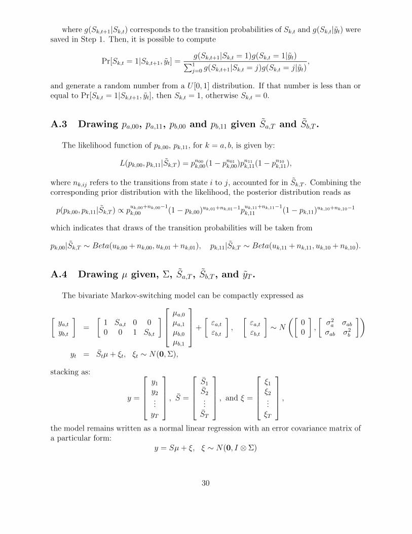
A.4 Drawing µ given, Σ, Sa,T , Sb,T , and yT .

The bivariate Markov-switching model can be compactly expressed as

[ya,tyb,t

]=

[10

Sa,t0

01

0Sb,t

]µa,0µa,1µb,0µb,1

+

[εa,tεb,t

],

[εa,tεb,t

]∼ N

([00

],

[σ2a

σab

σabσ2b

])

yt = Stµ+ ξt, ξt ∼ N(0,Σ),

stacking as:

y =

y1

y2...yT

, S =

S1

S2...ST

, and ξ =

ξ1

ξ2...ξT

,the model remains written as a normal linear regression with an error covariance matrix ofa particular form:

y = Sµ+ ξ, ξ ∼ N(0, I ⊗ Σ)

30

Using the corresponding likelihood function, the conditional posterior distribution forthe intercepts reads as:

µ|Sa,T , Sb,T ,Σ−1, yT ∼ N(µ, V µ),

where

V µ =

(V −1µ +

T∑t=1

S ′tΣ−1St

)−1

µ = V µ

(V −1µ µ+

T∑t=1

S ′tΣ−1yt

).

When drawing µ = (µa,0, µa,1, µb,0, µb,1)′, we impose the constraint that µa,1 > 0 and µb,1 > 0to ensure identification of the regimes in the model.

A.5 Drawing Σ given µ, Sa,T , Sb,T , and yT .

Conditional on the mean, state variables and the data, the conditional posterior distri-bution for the variance-covariance matrix parameters reads as:

Σ−1|Sa,T , Sb,T , µ, yT ∼ W (S−1, υ),

υ = T + υ

S = S +T∑t=1

(yt − Stµ

) (yt − Stµ

)′,

after Σ−1 is generated, the elements in Σ are recovered.

The above steps are iterated 7000 times, discarding the first 2000 iterations to mitigatethe effect of the initial conditions.

31

B Dynamic Model Averaging in Markov-Switching Mod-

els

To compute the time-varying weights associated to each Markov-switching model, wefollow an algorithm that combines the Hamilton filter with the prediction and updatingequations used in the dynamic model averaging approach in Raftery et al. (2010).

At any given period t, we compute the following steps for all the models under consid-eration:

• Step 1: Using the corresponding transition probabilities p(Skt |Skt−1), compute thepredicted regime probabilities for any given model k given past information ψt−1,P (Skt |Mt = k, ψt−1).12

P (Skt , Skt−1|ψt−1) = p(Skt |Skt−1)P (Skt−1|ψt−1) (30)

p(Skt |Mt = k, ψt−1) =∑Skt−1

P (Skt , Skt−1|ψt−1). (31)

Then, the marginal likelihood is calculated from the predicted probabilities:

fk(yt|ψt−1) =∑Skt

∑Skt−1

fk(yt|Skt , Skt−1, ψt−1)P (Skt , Skt−1|ψt−1) (32)

• Step 2: Let πt|t−1,k = P (Mt = k|ψt−1) be the predictive probability associatedwith the k-th Markov-switching model at time t given the information up to t − 1.Starting with an equal weight initial model probability P (M0), we consider threedifferent approaches to compute the model updated probability:

A) Likelihood-based approach: we follow the updating criterion of Raftery et al.(2010), which uses the marginal likelihood:

πt|t,k =πt|t−1,kfk(yt|ψt−1)∑Kj=1 πt|t−1,jfj(yt|ψt−1)

. (33)

B) Combined approach: we propose to use both types of information, i.e. the inversecumulative QPS and the marginal likelihood:

πt|t,k =πt|t−1,kfk(yt|ψt−1)/Qk,t|t∑Kj=1 πt|t−1,jfj(yt|ψt−1)/Qj,t|t

, (34)

where Qk,t|t = 2t

∑tτ=1(P (Skτ = 0|Mt = k, ψt)−NBERτ )

2.

12The Hamilton filter is initialized with the ergodic probabilities P (S0).

32

C) QPS-based approach: we also propose to use just the inverse of the cumulativeQPS instead of the likelihood, since the it focuses only on ability of models todetect regime shifts:

πt|t,k =πt|t−1,kQ

−1k,t|t∑K

j=1 πt|t−1,jQ−1j,t|t

. (35)

• Step 3: Use the marginal likelihood, fk(yt|ψt−1), to compute the updated regimeprobabilities for any given model k, P (Skt |Mt = k, ψt), as follows:

P (Skt , Skt−1|ψt) =

fk(yt, Skt , S

kt−1|ψt−1)

fk(yt|ψt−1)

=fk(yt|Skt , Skt−1, ψt−1)P (Skt , S

kt−1|ψt−1)

fk(yt|ψt−1)(36)

P (Skt |Mt = k, ψt) =∑Skt−1

P (Skt , Skt−1|ψt), (37)

which are used in Step 1 of the next iteration .

• Step 4: Compute the predicted probability associated to the k-th model, πt+1|t,k, byrelying on Raftery et al. (2010) and using the forgetting factor α, as follows:

πt+1|t,k =παt|t,k∑Kj=1 π

αt|t,j

, (38)

which are used in Step 2 of the next iteration .

We repeat the steps above for each model at each period of time t = 1, ..., T . The outputof the algorithm consists of the regimes probabilities for each model, P (Skt |Mt = k, ψt),and the model probabilities for each time period, πt|t,k = P (Mt = k|ψt). Therefore, wecompute the expected regime probabilities by averaging them across models:

P (St|ψt) =K∑k=1

P (Skt |Mt = k, ψt)P (Mt = k|ψt). (39)

The aggregated probability P (St|ψt) from the above equation is used to assess the perfor-mance of all models using the dynamic model averaging approach.

33

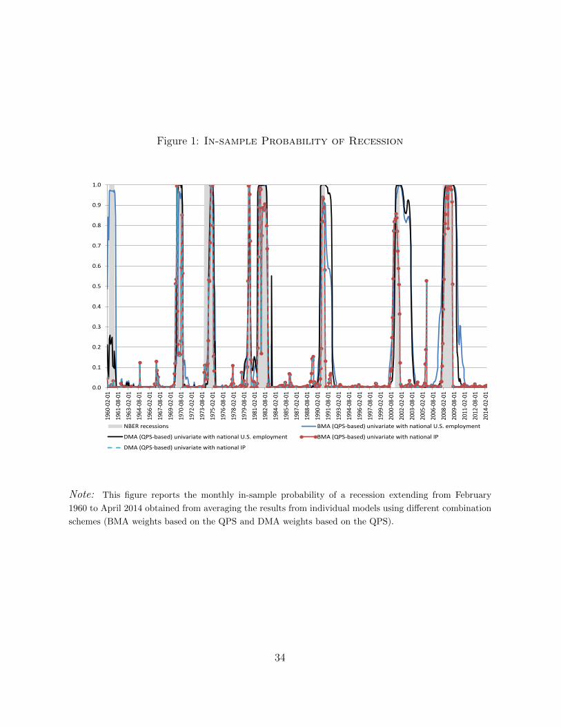
Figure 1: In-sample Probability of Recession

0.0

0.1

0.2

0.3

0.4

0.5

0.6

0.7

0.8

0.9

1.0

1960

-02-

0119

61-0

8-01

1963

-02-

0119

64-0

8-01

1966

-02-

0119

67-0

8-01

1969

-02-

0119

70-0

8-01

1972

-02-

0119

73-0

8-01

1975

-02-

0119

76-0

8-01

1978

-02-

0119

79-0

8-01

1981

-02-

0119

82-0

8-01

1984

-02-

0119

85-0

8-01

1987

-02-

0119

88-0

8-01

1990

-02-

0119

91-0

8-01

1993

-02-

0119

94-0

8-01

1996

-02-

0119

97-0

8-01

1999

-02-

0120

00-0

8-01

2002

-02-

0120

03-0

8-01

2005

-02-

0120

06-0

8-01

2008

-02-

0120

09-0

8-01

2011

-02-

0120

12-0

8-01

2014

-02-

01

NBER recessions BMA (QPS-based) univariate with national U.S. employment

DMA (QPS-based) univariate with national U.S. employment BMA (QPS-based) univariate with national IP

DMA (QPS-based) univariate with national IP

Note: This figure reports the monthly in-sample probability of a recession extending from February

1960 to April 2014 obtained from averaging the results from individual models using different combination

schemes (BMA weights based on the QPS and DMA weights based on the QPS).

34

Figure 2: In-sample model weights from dynamic model averaging(likelihood-based)

0

0.1

0.2

0.3

0.4

0.5

0.6

0.7

0.8

0.9

11

96

0-0

2-0

1

19

61

-05

-01

19

62

-08

-01

19

63

-11

-01

19

65

-02

-01

19

66

-05

-01

19

67

-08

-01

19

68

-11

-01

19

70

-02

-01

19

71

-05

-01

19

72

-08

-01

19

73

-11

-01

19

75

-02

-01

19

76

-05

-01

19

77

-08

-01

19

78

-11

-01

19

80

-02

-01

19

81

-05

-01

19

82

-08

-01

19

83

-11

-01

19

85

-02

-01

19

86

-05

-01

19

87

-08

-01

19

88

-11

-01

19

90

-02

-01

19

91

-05

-01

19

92

-08

-01

19

93

-11

-01

19

95

-02

-01

19

96

-05

-01

19

97

-08

-01

19

98

-11

-01

20

00

-02

-01

20

01

-05

-01

20

02

-08

-01

20

03

-11

-01

20

05

-02

-01

20

06

-05

-01

20

07

-08

-01

20

08

-11

-01

20

10

-02

-01

20

11

-05

-01

20

12

-08

-01

20

13

-11

-01

Panel A. Employment

AL AK AZ AR CA CO CT DE FL GA HI ID IL

IN IA KS KY LA ME MD MA MI MN MS MO MT

NE NV NH NJ NM NY NC ND OH OK OR PA RI

SC SD TN TX UT VT VA WA WI WV WY

0

0.05

0.1

0.15

0.2

0.25

0.3

0.35

0.4

19

60

-02

-01

19

61

-06

-01

19

62

-10

-01

19

64

-02

-01

19

65

-06

-01

19

66

-10

-01

19

68

-02

-01

19

69

-06

-01

19

70

-10

-01

19

72

-02

-01

19

73

-06

-01

19

74

-10

-01

19

76

-02

-01

19

77

-06

-01

19

78

-10

-01

19

80

-02

-01

19

81

-06

-01

19

82

-10

-01

19

84

-02

-01

19

85

-06

-01

19

86

-10

-01

19

88

-02

-01

19

89

-06

-01

19

90

-10

-01

19

92

-02

-01

19

93

-06

-01

19

94

-10

-01

19

96

-02

-01

19

97

-06

-01

19

98

-10

-01

20

00

-02

-01

20

01

-06

-01

20

02

-10

-01

20

04

-02

-01

20

05

-06

-01

20

06

-10

-01

20

08

-02

-01

20

09

-06

-01

20

10

-10

-01

20

12

-02

-01

20

13

-06

-01

Panel B. Industrial Production

AL AK AZ AR CA CO CT DE FL GA HI ID IL

IN IA KS KY LA ME MD MA MI MN MS MO MT

NE NV NH NJ NM NY NC ND OH OK OR PA RI

SC SD TN TX UT VT VA WA WI WV WY

Note: This figure reports the weights obtained when averaging the results from univariate models using

DMA weights based on the likelihood (with forgetting factor α = 0.99). Panel A shows the results when

using employment as a measure of national economic activity and panel B when using industrial production

as a measure of national economic activity.

35

Figure 3: In-sample model weights from dynamic model averaging (qps-based)

0

0.1

0.2

0.3

0.4

0.5

0.6

0.7

0.8

0.9

1

19

60

-02

-01

19

61

-06

-01

19

62

-10

-01

19

64

-02

-01

19

65

-06

-01

19

66

-10

-01

19

68

-02

-01

19

69

-06

-01

19

70

-10

-01

19

72

-02

-01

19

73

-06

-01

19

74

-10

-01

19

76

-02

-01

19

77

-06

-01

19

78

-10

-01

19

80

-02

-01

19

81

-06

-01

19

82

-10

-01

19

84

-02

-01

19

85

-06

-01

19

86

-10

-01

19

88

-02

-01

19

89

-06

-01

19

90

-10

-01

19

92

-02

-01

19

93

-06

-01

19

94

-10

-01

19

96

-02

-01

19

97

-06

-01

19

98

-10

-01

20

00

-02

-01

20

01

-06

-01

20

02

-10

-01

20

04

-02

-01

20

05

-06

-01

20

06

-10

-01

20

08

-02

-01

20

09

-06

-01

20

10

-10

-01

20

12

-02

-01

20

13

-06

-01

Panel A. Employment

AL AK AZ AR CA CO CT DE FL GA HI ID IL

IN IA KS KY LA ME MD MA MI MN MS MO MT

NE NV NH NJ NM NY NC ND OH OK OR PA RI

SC SD TN TX UT VT VA WA WI WV WY

0

0.1

0.2

0.3

0.4

0.5

0.6

0.7

0.8

0.9

1

19

60

-02

-01

19

61

-05

-01

19

62

-08

-01

19

63

-11

-01

19

65

-02

-01

19

66

-05

-01

19

67

-08

-01

19

68

-11

-01

19

70

-02

-01

19

71

-05

-01

19

72

-08

-01

19

73

-11

-01

19

75

-02

-01

19

76

-05

-01

19

77

-08

-01

19

78

-11

-01

19

80

-02

-01

19

81

-05

-01

19

82

-08

-01

19

83

-11

-01

19

85

-02

-01

19

86

-05

-01

19

87

-08

-01

19

88

-11

-01

19

90

-02

-01

19

91

-05

-01

19

92

-08

-01

19

93

-11

-01

19

95

-02

-01

19

96

-05

-01

19

97

-08

-01

19

98

-11

-01

20

00

-02

-01

20

01

-05

-01

20

02

-08

-01

20

03

-11

-01

20

05

-02

-01

20

06

-05

-01

20

07

-08

-01

20

08

-11

-01

20

10

-02

-01

20

11

-05

-01

20

12

-08

-01

20

13

-11

-01

Panel B. Industrial Production

AL AK AZ AR CA CO CT DE FL GA HI ID IL

IN IA KS KY LA ME MD MA MI MN MS MO MT

NE NV NH NJ NM NY NC ND OH OK OR PA RI

SC SD TN TX UT VT VA WA WI WV WY

Note: This figure reports the weights obtained when averaging the results from univariate models using

DMA weights based on the QPS (with forgetting factor α = 0.99). Panel A shows the results when using

employment as a measure of national economic activity and panel B when using industrial production as

a measure of national economic activity.

36

Figure 4: In-sample model weights from dynamic model averaging (Combined)

0

0.1

0.2

0.3

0.4

0.5

0.6

0.7

0.8

0.9

1

1960

-02-

0119

61-0

5-01

1962

-08-

0119

63-1

1-01

1965

-02-

0119

66-0

5-01

1967

-08-

0119

68-1

1-01

1970

-02-

0119

71-0

5-01

1972

-08-

0119

73-1

1-01

1975

-02-

0119

76-0

5-01

1977

-08-

0119

78-1

1-01

1980

-02-

0119

81-0

5-01

1982

-08-

0119

83-1

1-01

1985

-02-

0119

86-0

5-01

1987

-08-

0119

88-1

1-01

1990

-02-

0119

91-0

5-01

1992

-08-

0119

93-1

1-01

1995

-02-

0119

96-0

5-01

1997

-08-

0119

98-1

1-01

2000

-02-

0120

01-0

5-01

2002

-08-

0120

03-1

1-01

2005

-02-

0120

06-0

5-01

2007

-08-

0120

08-1

1-01

2010

-02-

0120

11-0

5-01

2012

-08-

0120

13-1

1-01

Panel A. Employment

AL AK AZ AR CA CO CT DE FL GA HI ID IL

IN IA KS KY LA ME MD MA MI MN MS MO MT

NE NV NH NJ NM NY NC ND OH OK OR PA RI

SC SD TN TX UT VT VA WA WI WV WY

0

0.1

0.2

0.3

0.4

0.5

0.6

0.7

0.8

0.9

1

1960

-02-

0119

61-0

6-01

1962

-10-

0119

64-0

2-01

1965

-06-

0119

66-1

0-01

1968

-02-

0119

69-0

6-01

1970

-10-

0119

72-0

2-01

1973

-06-

0119

74-1

0-01

1976

-02-

0119

77-0

6-01

1978

-10-

0119

80-0

2-01

1981

-06-

0119

82-1

0-01

1984

-02-

0119

85-0

6-01

1986

-10-

0119

88-0

2-01

1989

-06-

0119

90-1

0-01

1992

-02-

0119

93-0

6-01

1994

-10-

0119

96-0

2-01

1997

-06-

0119

98-1

0-01

2000

-02-

0120

01-0

6-01

2002

-10-

0120

04-0

2-01

2005

-06-

0120

06-1

0-01

2008

-02-

0120

09-0

6-01

2010

-10-

0120

12-0

2-01

2013

-06-

01

Panel B. Industrial Production

AL AK AZ AR CA CO CT DE FL GA HI ID IL

IN IA KS KY LA ME MD MA MI MN MS MO MT

NE NV NH NJ NM NY NC ND OH OK OR PA RI

SC SD TN TX UT VT VA WA WI WV WY

Note: This figure reports the weights obtained when averaging the results from univariate models using

DMA weights based on a combination of QPS and predictive likelihood (with forgetting factor α = 0.99).

Panel A shows the results when using employment as a measure of national economic activity and panel

B when using industrial production as a measure of national economic activity.

37

Figure 5: In-sample model weights from Bayesian model averaging

0

0.1

0.2

0.3

0.4

0.5

0.6

0.7

0.8

0.9

1

0

0.02

0.04

0.06

0.08

0.1

0.12

0.14

AL

AK AZ

AR

CA CO CT DE FL GA HI

ID IL IN IA KS KY LA ME

MD

MA MI

MN

MS

MO

MT

NE

NV

NH NJ

NM NY

NC

ND

OH

OK

OR

PA RI

SC SD TN TX UT

VT

VA

WA

WI

WV

WY

Panel A. Employment

BMA (QPS-based) [left axis] BMA (Likelihood-based) [right axis]

0

0.1

0.2

0.3

0.4

0.5

0.6

0.7

0.8

0.9

1

0

0.02

0.04

0.06

0.08

0.1

0.12

0.14

AL

AK AZ

AR

CA CO CT DE FL GA HI

ID IL IN IA KS KY LA ME

MD

MA MI

MN

MS

MO

MT

NE

NV

NH NJ

NM NY

NC

ND

OH

OK

OR

PA RI

SC SD TN TX UT

VT

VA

WA

WI

WV

WY

Panel B. Industrial Production

BMA (QPS-based) [left axis] BMA (Likelihood-based) [right axis]

Note: This figure reports the weights obtained when averaging the results from univariate models using

BMA weights based on the QPS and marginal likelihood. Panel A shows the results when using employment

as a measure of national economic activity and panel B when using industrial production as a measure of

national economic activity.

38

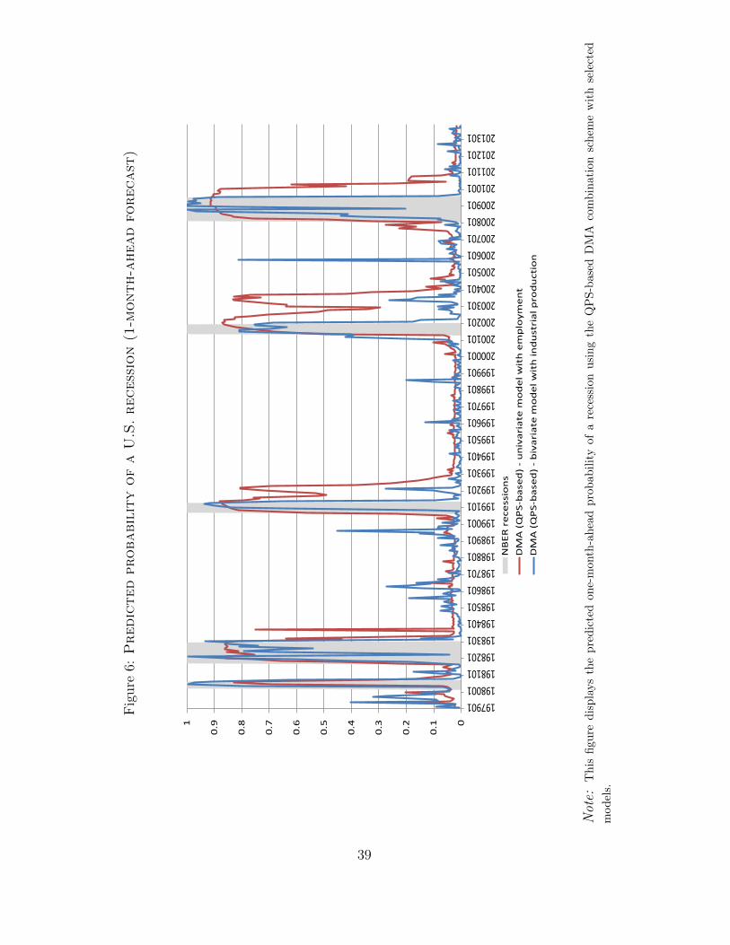
Fig

ure

6:Predicted

probabilityofaU.S.recession(1-m

onth-ahead

forecast

)

0

0.1

0.2

0.3

0.4

0.5

0.6

0.7

0.8

0.91

197901198001198101198201198301198401198501198601198701198801198901199001199101199201199301199401199501199601199701199801199901200001200101200201200301200401200501200601200701200801200901201001201101201201201301

NB

ER r

ece

ssio

ns

DM

A (

QP

S-b

ase

d)

- u

niv

aria

te m

od

el w

ith

em

plo

yme

nt

DM

A (

QP

S-b

ase

d)

- b

ivar

iate

mo

de

l wit

h in

du

stri

al p

rod

uct

ion

Note:

Th

isfi

gure

dis

pla

ys

the

pre

dic

ted

one-

month

-ah

ead

pro

bab

ilit

yof

are

cess

ion

usi

ng

the

QP

S-b

ase

dD

MA

com

bin

ati

on

sch

eme

wit

hse

lect

ed

mod

els.

39

Fig

ure

7:Real-tim

eprobabilityofaU.S.recession

0

0.1

0.2

0.3

0.4

0.5

0.6

0.7

0.8

0.91

2007-05-01

2007-08-01

2007-11-01

2008-02-01

2008-05-01

2008-08-01

2008-11-01

2009-02-01

2009-05-01

2009-08-01

2009-11-01

2010-02-01

2010-05-01

2010-08-01

2010-11-01

2011-02-01

2011-05-01

2011-08-01

2011-11-01

2012-02-01

2012-05-01

2012-08-01

2012-11-01

2013-02-01

2013-05-01

2013-08-01

NB

ER r

ece

ssio

ns

SPF

An

xio

us

ind

ex

Biv

aria

te m

od

el w

ith

nat

ion

al IP

Un

ivar

iate

mo

de

l wit

h n

atio

nal

em

plo

yme

nt

Note:

Th

isfi

gure

dis

pla

ys

the

real

-tim

ep

rob

abil

ity

of

are

cess

ion

usi

ng

the

QP

S-b

ase

dD

MA

com

bin

ati

on

sch

eme

(un

ivari

ate

mod

elw

ith

emp

loym

ent

and

biv

aria

tem

od

elw

ith

ind

ust

rial

pro

du

ctio

n)

alo

ng

wit

hth

ep

rob

ab

ilit

yof

rece

ssio

nd

eriv

edfr

om

the

Su

rvey

of

Pro

fess

ion

al

Fore

cast

ers

(SP

F).

Th

e

vert

ical

bar

sin

dic

ate

the

dat

esof

the

NB

ER

ann

ou

nce

men

tsof

the

bu

sin

ess

cycl

ep

eak

an

dtr

ou

gh

.

40