Particle Filters for Markov-SwitchingStochastic-Correlation Models

Giannni Amisano1Dep. of Economics, University of Brescia

European Central BankE-mail: amisano@eco.unibs.it

Roberto Casarin2Dep. of Economics, University of Brescia,

Dep. of Mathematics, University Paris DauphineE-mail: casarin@eco.unibs.it

Abstract: This work deals with multivariate stochastic volatility models that account fortime-varying stochastic correlation between the observable variables. We focus on thebivariate models. A contribution of the work is to introduceBeta and Gamma autoregres-sive processes for modelling the correlation dynamics. Another contribution of our workis to allow the parameter of the correlation process to be governed by a Markov-switchingprocess. Finally we propose a simulation-based Bayesian approach, called regularisedsequential Monte Carlo. This framework is suitable for on-line estimation and the modelselection.

Keywords: Markov Switching; Stochastic Correlation; Multivariate Stochastic Volatility;Particle Filters; Sequential Monte Carlo; Beta Autoregressive Process

1. Introduction

After the introduction of theDynamic Conditional Correlation(DCC) model due to En-gle (2002), the literature mainly focuses on the application of a time-varying correlationstructure to the class of multivariate GARCH models. For an updated review on multi-variate GARCH models we refer to Bauwenset al. (2006).In stochastic volatility modeling, the results obtained inthe univariate case (see for exam-ple Taylor (1986, 1994) and Jacquieret al.(1994)) have been extended to the multivariatecase (see Harveyet al. (1994), Aguilar and West (2000) and Chibet al. (2006)) by con-sidering a constant correlation structure. See also Asai and McAleer (2006a) and Asaiet al. (2006) for an updated review onMultivariate Stochastic VolatilityMSV.Recent studies start dealing with time-varying correlation in MSV models. The modelsdue to Philipov and Glickman (2006) and Gourierouxet al.(2004) allow for time-varyingvariances and covariances. However the stochastic correlation structure is implicitly de-termined by the dynamics of variances and covariances, thusa direct modeling of thecorrelation between asset returns is not possible. In this work we follow instead an al-ternative route. We treat variances and correlations separately. This allows us to better

2Address of correspondence: Dep. of Economics, University of Brescia, San Faustino, 74/b, 25122Brescia, Italy

describe the dynamics of the two set of variables and the causality relations between them.For an updated discussion on the different ways of introducing time-varying correlationinto MSV models see Asai and McAleer (2006b, 2005).In our stochastic-correlation MSV models both the variancevector and the correlation ma-trix are stochastic unobservable (or latent) variables. The use of latent variables allows amore flexible modeling of the volatility and correlation dynamics than the DCC-GARCHapproach. Unobservable components provide a natural setting to introduce exogenousexplanatory variables in the correlation and variance dynamics. Nevertheless stochasticcorrelation MSV models are difficult to estimate and a suitable inference approach is theobject of many latter works.The first aim of our work is to propose new classes of stochastic models for represent-ing the correlation dynamics. We propose the use ofGamma Autoregressive Processesdue to Gourieroux and Jasiak (2006) and of theBeta Autoregressive Processes(BAR),which have the advantage to be naturally defined on a bounded interval. BAR are weakautoregressive processes and, similarly to the Gamma autoregressive, can accomodatevarious nonlinearities in the correlation dynamics. Our approach borrows from the ear-lier Bayesian literature on hazard rate modeling (see Nieto-Barajas and Walker (2002)),and on the construction of general autoregressive processes (see Mena and Walker (2004)and Pittet al. (2002)), but represents an original application to the dynamic correlationmodeling.Another contribution of the paper is to introduce a new classof models which account forsudden changes of regimes in the correlation dynamics. The proposed stochastic correla-tion models can be extended by considering heavy-tailed observation noise. We proposeskewed Student-t distributions, which allow for different magnitude of kurtosis and skew-ness in each direction of the observation space.The last aim of our work is to apply a full Bayesian approach tothe sequential estima-tion of the unknown parameter and to the nonlinear filtering problem which arises whenestimating the hidden states. The Bayesian inference approach is powerful in dealingwith the estimation of nonlinear models (Jacquieret al. (1994)). The existing literatureon Bayesian inference for MSV and for dynamic correlation models mainly focused ontraditional MCMC methods (see Asai and McAleer (2006a)). Inthe Bayesian framework,alternative estimation methods have been recently proposed. These methods rely upon aconvenient nonlinear state-space representation of the econometric model of interest anduponSequential Monte Carlo(SMC) techniques also calledParticle Filter (PF). SMCallows to deal with nonlinear state-space models and is particularly suitable for on-lineapplications (see Doucetet al. (2001), Pitt and Shephard (1999), Polsonet al. (2002,2003)).The work is organised as follows. Section 2 first defines bivariate stochastic volatilitymodels. Then stochastic correlation models, such as Gamma and Beta autoregressiveprocesses are introduced. Finally the Markov-switching correlation is considered. Section3 presents the particle filter approach to the on-line estimation of the latent variables andthe unknown parameters and for the selection of the model. Section 4 concludes.

2. Markov-Switching Stochastic-Correlation

Let yt = (y1t, y2t)′ ∈ R

2 be a2-dimensional vector of observable variables andht =(h1t, h2t)

′ ∈ R2 a2-dimensional vector of stochastic log-volatilities. Denote the stochastic

correlation matrix byΩt and letΛt = diagexp(h1t/2), exp(h2t/2) be a diagonal matrixwith standard deviations on the main diagonal. The time-varying variance-covariancematrix of the observable factorises as follow:Σt = ΛtΩtΛt. Note that this decompositionallows us to model volatilities and correlations separately.The proposed multivariate stochastic volatility model is

yt = Ayt−1 + Σ1/2t εt, εt ∼ N2 (0, Id2) (1)

ht+1 = c +Bht + Ξ1/2ηt, ηt ∼ N2 (0, Id2) (2)

whereεt ⊥ ηs, ∀ s, t, which denotes the absence of leverage.Idn represents then-dimensional identity matrix andNn (0, Idn) then-variate standard normal.Ξ1/2 denotesthe Cholesky decomposition ofΞ, which represents the variance-covariance matrix of thelog-volatility process and captures instantaneous spill-over effects across asset volatilities.The autoregressive coefficientB is constant and determines the causality structure (spill-over effects) in the log-volatility. In the following we focus on the dynamic of the sto-chastic correlation.Let (st)t≥0 be a univariate Markov-switching process with values inE = 1, . . . , L ⊂ N

and transition density

P(st+1 = i|st = j) = pij , with i, j ∈ E. (3)

Let (ψt)t≥0 be a sequence of i.i.d. white noises. In this work we assume:ψt ⊥ εs andψt ⊥ ηs, ∀ s, t, but the proposed model and inference framework can be extended toinclude dependence between those processes.The(i, j)-th element of the stochastic correlation matrixΩt is defined as follows

ρij,t = (1 − δi(j))φ(ωt) + δi(j) (4)

ωt+1 = g(ωt, st+1, ψt) (5)

with i, j ∈ 1, 2 andφ : R → [−1,+1] a smooth function. In the previous equationωt is a latent process (customarily calledtransformed correlation process) driving thecorrelation between observable processes. The functiong : (R × E × R) → R definesthe transition dynamics ofωt.In the following examples we discus some stochastic correlation models. In particular wefocus on some alternative ways to specify the stochastic correlation process. We show alsohow to introduce a switching-regimes process in the dynamics of the correlation process.

Example 1- (Switching Gaussian Autoregressive)We assume the transformed correlation processωt follows a Markov-switching first orderGaussian autoregressive process

ωt+1 = ωst+1+ λst+1

ωt + γ1/2st+1

ψt, ψt ∼ N (0, 1), (6)

with γk > 0, ∀k. Note that our model has the pure Markov-switching correlation processas a special case, whenλk = 0 andγk = 0 ∀k.In order to obtain a process which lives in the interval[−1,+1], we could apply toωt theFisher’s transform

φ(ωt) =exp(ωt) − 1

exp(ωt) + 1,

. A simulated example of Markov-switching stochastic-correlation is given in Fig. 1.

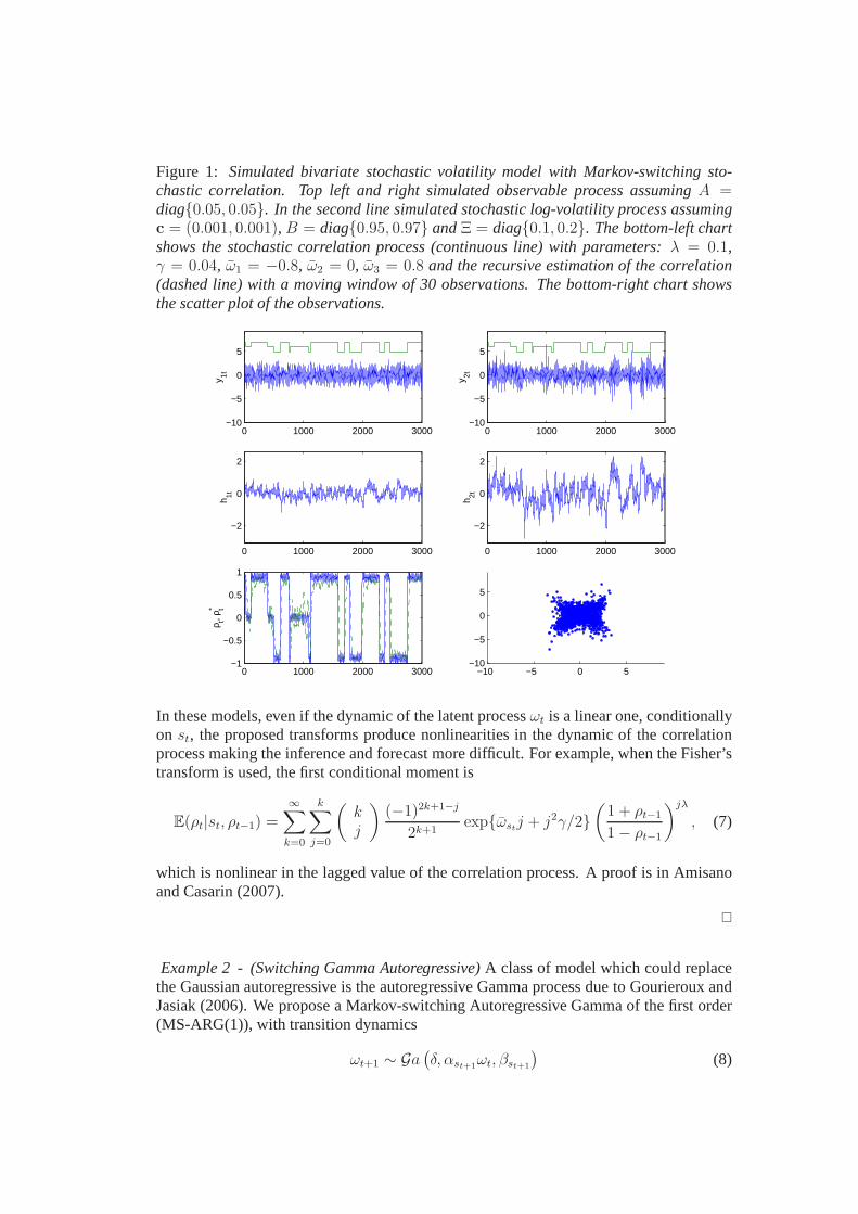
Figure 1: Simulated bivariate stochastic volatility model with Markov-switching sto-chastic correlation. Top left and right simulated observable process assumingA =diag0.05, 0.05. In the second line simulated stochastic log-volatility process assumingc = (0.001, 0.001),B = diag0.95, 0.97 andΞ = diag0.1, 0.2. The bottom-left chartshows the stochastic correlation process (continuous line) with parameters:λ = 0.1,γ = 0.04, ω1 = −0.8, ω2 = 0, ω3 = 0.8 and the recursive estimation of the correlation(dashed line) with a moving window of 30 observations. The bottom-right chart showsthe scatter plot of the observations.

0 1000 2000 3000−10

−5

0

5

y 1t

0 1000 2000 3000−10

−5

0

5

y 2t

0 1000 2000 3000

−2

0

2

h 1t

0 1000 2000 3000

−2

0

2h 2t

0 1000 2000 3000−1

−0.5

0

0.5

1

ρ t, ρ* t

−10 −5 0 5−10

−5

0

5

In these models, even if the dynamic of the latent processωt is a linear one, conditionallyon st, the proposed transforms produce nonlinearities in the dynamic of the correlationprocess making the inference and forecast more difficult. For example, when the Fisher’stransform is used, the first conditional moment is

E(ρt|st, ρt−1) =

∞∑

k=0

k∑

j=0

(

kj

)

(−1)2k+1−j

2k+1expωst

j + j2γ/2

(

1 + ρt−1

1 − ρt−1

)jλ

, (7)

which is nonlinear in the lagged value of the correlation process. A proof is in Amisanoand Casarin (2007).

Example 2- (Switching Gamma Autoregressive)A class of model which could replacethe Gaussian autoregressive is the autoregressive Gamma process due to Gourieroux andJasiak (2006). We propose a Markov-switching Autoregressive Gamma of the first order(MS-ARG(1)), with transition dynamics

ωt+1 ∼ Ga(

δ, αst+1ωt, βst+1

)

(8)

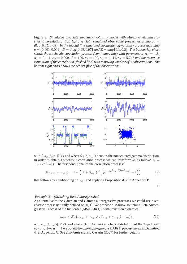
Figure 2: Simulated bivariate stochastic volatility model with Markov-switching sto-chastic correlation. Top left and right simulated observable process assumingA =diag0.05, 0.05. In the second line simulated stochastic log-volatility process assumingc = (0.001, 0.001),B = diag0.95, 0.97 andΞ = diag0.1, 0.2. The bottom-left chartshows the stochastic correlation process (continuous line) with parameters:α1 = 1.8,α2 = 0.111, α3 = 0.009, β = 100, γ1 = 100, γ2 = 11.11, γ1 = 5.747 and the recursiveestimation of the correlation (dashed line) with a moving window of 30 observations. Thebottom-right chart shows the scatter plot of the observations.

0 1000 2000 3000

−5

0

5

10

y 1t

0 1000 2000 3000

−5

0

5

10

y 2t

0 1000 2000 3000

−2

−1

0

1

2

h 1t

0 1000 2000 3000

−2

−1

0

1

2h 2t

0 1000 2000 3000−1

−0.5

0

0.5

1

ρ t, ρ* t

−5 0 5

−5

0

5

with δ, αk, βk ∈ R ∀k and whereGa(δ, α, β) denotes the noncentered gamma distribution.In order to obtain a stochastic correlation process we can transformωt as follow: ρt =1 − exp(−ωt). The first conditional of the correlation process is

E(ρt+1|ρt, st+1) = 1 −(

(1 + βst+1)−δ

(

ραst+1

βst+1/(1+βst+1

)

t − 1))

(9)

that follows by conditioning onst+1 and applying Proposition 4..2 in Appendix B.

Example 3- (Switching Beta Autoregressive)As alternative to the Gaussian and Gamma autoregressive processes we could use a sto-chastic process naturally defined on[0, 1]. We propose a Markov-switching Beta Autore-gressive Process of the first order (MS-BAR(1)), with transition dynamics

ωt+1 ∼ Be(

αst+1+ γst+1

ωt, βst+1+ γst+1

(1 − ωt))

, (10)

with αk, βk, γk ∈ R ∀k and whereBe(a, b) denotes a beta distribution of the Type I witha, b > 0. ForK = 1 we obtain the time-homogeneous BAR(1) process given in Definition4..2, Appendix C. See also Amisano and Casarin (2007) for further details.

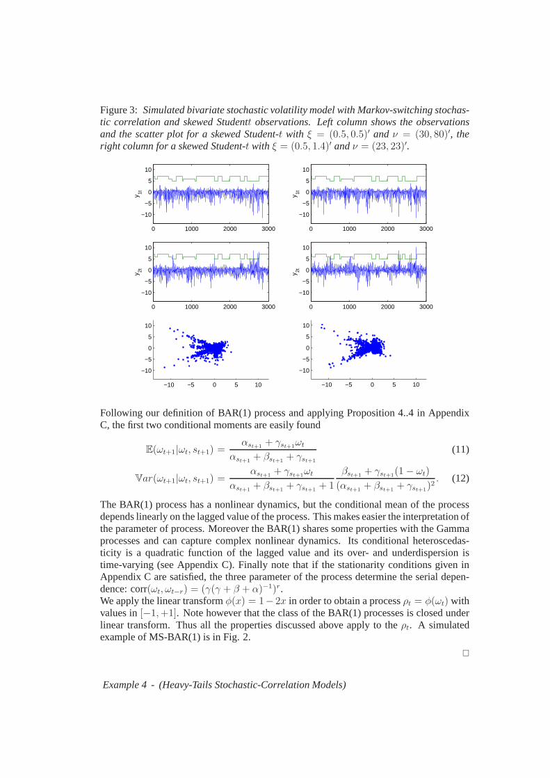
Figure 3: Simulated bivariate stochastic volatility model with Markov-switching stochas-tic correlation and skewed Studentt observations. Left column shows the observationsand the scatter plot for a skewed Student-t with ξ = (0.5, 0.5)′ and ν = (30, 80)′, theright column for a skewed Student-t with ξ = (0.5, 1.4)′ andν = (23, 23)′.

0 1000 2000 3000

−10

−5

0

5

10

y 1t

0 1000 2000 3000

−10

−5

0

5

10

y 1t

0 1000 2000 3000

−10

−5

0

5

10

y 2t

0 1000 2000 3000

−10

−5

0

5

10

y 2t

−10 −5 0 5 10

−10

−5

0

5

10

−10 −5 0 5 10

−10

−5

0

5

10

Following our definition of BAR(1) process and applying Proposition 4..4 in AppendixC, the first two conditional moments are easily found

E(ωt+1|ωt, st+1) =αst+1

+ γst+1ωt

αst+1+ βst+1

+ γst+1

(11)

Var(ωt+1|ωt, st+1) =αst+1

+ γst+1ωt

αst+1+ βst+1

+ γst+1+ 1

βst+1+ γst+1

(1 − ωt)

(αst+1+ βst+1

+ γst+1)2. (12)

The BAR(1) process has a nonlinear dynamics, but the conditional mean of the processdepends linearly on the lagged value of the process. This makes easier the interpretation ofthe parameter of process. Moreover the BAR(1) shares some properties with the Gammaprocesses and can capture complex nonlinear dynamics. Its conditional heteroscedas-ticity is a quadratic function of the lagged value and its over- and underdispersion istime-varying (see Appendix C). Finally note that if the stationarity conditions given inAppendix C are satisfied, the three parameter of the process determine the serial depen-dence: corr(ωt, ωt−r) = (γ(γ + β + α)−1)r.We apply the linear transformφ(x) = 1− 2x in order to obtain a processρt = φ(ωt) withvalues in[−1,+1]. Note however that the class of the BAR(1) processes is closed underlinear transform. Thus all the properties discussed above apply to theρt. A simulatedexample of MS-BAR(1) is in Fig. 2.

Example 4- (Heavy-Tails Stochastic-Correlation Models)

As alternative to the Gaussian VAR process we could use a process which account alsofor skewness and kurtosis. We propose a skewed Student-t model

yt = Atyt−1 + Σ1/2t εt, εt ∼ SkT2 (0, Id2, ν, ξ) (13)

ht+1 = c +Bht + Ξ1/2ηt, ηt ∼ N2 (0, Id2) (14)

whereSkTn (0, Idn, ν, ξ) is then-variate skewed Student-t with ν = (ν1, . . . , νn)′ de-grees of freedom vector and skewness parameterξ = (ξ1, . . . , ξn)

′. For a definition ofmultivariate skewed Student-t distribution see Azzalini and Dalla Valle (1996), Brancoand Dey (2001) and Sahuet al. (2003). In this work we adopt the definition due toFerreira and Steel (2003) (but see also Bauwens and Laurent (2002) for a quite similardefinition). Their constructive method for skewed Student-t makes the simulation fromthis distribution simple. The existence of the moments is guaranteed by the existence ofthe moments of the underlying univariate distributions. Finally the resulting multivariatedistribution accounts for heterogenous components, i.e. it allows for different magnitudesand directions of kurtosis and skewness. Two simulated examples of skewed Student-tobservations are given in Fig. 3.

3. Bayesian Inference

3.1 Estimation of Latent Variables and Parameters

In the following we deal with the inference problems in the nonlinear dynamic modelspresented in previous sections. We follow the nonlinear filtering approach. As suggestedby Berzuiniet al.(1997) we include the parameters into the state vector and then, follow-ing Liu and West (2001), we apply aRegularised Auxiliary Particle Filter(R-APF) forfiltering the hidden states and estimating the unknown parameters of the model.We assume that the Bayesian nonlinear model is represented in a distributional state-spaceform, that is defined by the following measurement, transition and initial densities

yt ∼ p(yt|xt, θt) (15)

(xt, θt) ∼ p(xt, θt|xt−1, θt−1) (16)

(x0, θ0) ∼ p(x0|θ0)p(θ0) (17)

with t = 1, 2, . . . , T . In this general and possibly nonlinear model,yt ∈ Y ⊂ Rny

represents the observable variable,Y the observations space,xt ∈ X ⊂ Rnx the hidden

state (i.e. the latent variable) andX the state space.We assume the transition density of the parameter vector is trivially δθt−1

(θt), whereδx(y)denotes the Dirac’s mass centered inx. The last line shows the prior distribution on theparameter vectorθ0 = θ, with θ ∈ Θ ⊂ R

nθ . Note that the prior distribution on theparameter represents the Bayesian part of the model.In the case of the three-regime models given in the previous examples,yt ∈ R

2 andxt = (h′

t, ωt, st)′ ∈ (R2 × R × 1, 2, 3). The parameter vectors in examples 1 and 3

areθ = ((a11, a22)′, c′, (b11, b22)

′, vecΞ′, λ, γ, ω1, ω2, ω3)′ andθ = ((a11, a22)

′, c′,(b11, b22)

′, vecΞ′, λ, α1, α2, α3, β, γ1, γ2, γ3)′ respectively. We denote withvec the

matrix operator, which stacks into a vector the columns of a given matrix.

Let us definezt = (x′t, θ

′t)

′, Z = X × Θ andzs:t = (zs, zs+1, . . . , zt). The optimalprediction, filtering and smoothing densities, for the model in Eq. (15), (16) and (17), are

p(zt+1|y1:t) =

∫

Z

p(xt+1|xt, θt+1)δθt(θt+1)p(zt|y1:t)dzt (18)

p(yt+1|y1:t) =

∫

Z

p(yt+1|zt+1)p(zt|y1:t)dzt+1 (19)

p(zt+1|y1:t+1) =p(yt+1|xt+1, θt+1)p(xt+1|xt, θt+1)δθt

(θt+1)

p(yt+1|y1:t)(20)

p(zs|y1:t) = p(zs|y1:s)

∫

Z

(zs+1|zs)p(zs+1|y1:t)

p(zs+1|y1:t)dzs+1 (21)

with s < t.The analytical solution of the general stochastic filteringproblem described in Eq. (18)-(21) is known in only few cases. Inference problems in nonlinear and/or non-Gaussianstate-space models are usually solved by introducing some approximations. In this workwe bring into actionParticle Filters (PF) (Doucetet al. (2001)). In particular we applythe regularised particle filters due to Liu and West (2001) and Mussoet al. (2001).Let (zi

0, wi0) be a weighted sample from the prior distribution given in Eq.(17). The sam-

ple is also called particle and the collection ofN samples,zi0, w

i0

Ni=1 is called particle

set. Assume that at timet a particle setzit, w

it

Ni=1 is approximating the density in Eq.

(20), then the density in Eq. (18) is approximated

pN(zt+1|y1:t) ∝N

∑

i=1

1

N |H it |dwi

tp(zt+1|zit)KHi

t(zt+1 − zi

t) (22)

pN(yt+1|y1:t) ∝N

∑

i=1

1

N |H it |

dwi

tp(yt+1|xt+1, θt+1)KHit(zt+1 − zi

t) (23)

pN(zt+1|y1:t+1) ∝N

∑

i=1

1

N |H it |dwi

tp(yt+1|zt+1) (24)

whereKH(x) = K(H−1x) is a multivariate Gaussian kernel andH a p.d. scale matrix(bandwidth). |H| denotes the determinant ofH. Note that with respect to Liu and West(2001), we consider a matrix-variate bandwidths to allow for different jittering dimensionin each direction of the augmented state space. See Amisano and Casarin (2007) fordetails.

3.2 Number of Regimes

Let Lt represent the current number of regimes. Following Chopin Chopin (2001) andChopin and Pelgrin Chopin and Pelgrin (2004), the state vector is augmented with theauxiliary variable,mt+1 defined as follows

mt+1 = maxLt+1, mt (25)

This augmented state allow us to estimate sequentially the number of regimes. SeeAmisano and Casarin (2007) for further details.

4. Conclusion

We introduce some new Markov-switching stochastic-correlation models. For the infer-ence, a simulation-based Bayesian approach is considered,which relies upon sequentialMonte Carlo algorithms. SMC is particularly suitable for on-line model selection andjoint estimation of the latent variables and the parameters. The on-line context allows usto evaluate sequentially also risk and the performance of the optimal portfolio when thestochastic correlation is governed by a Markov-switching process.

References

Aguilar O. and West M. (2000) Bayesian Dynamic Factor Modelsand Portfolio Alloca-tion, Journal of Business and Economic Statistics, 18, 338–357.

Amisano G. and Casarin R. (2007) Particle filters for markov-switching stochastic-correlation models.

Arulampalam S., Maskell S., Gordon N. and Clapp T. (2001) A Tutorial on Particle Filtersfor On-line Nonlinear/Non-Gaussian Bayesian Tracking.

Asai M. and McAleer M. (2005) Dynamic Correlations in Symmetric Multivariate SVModels, in: MODSIM 2005 International Congress on Modelling and Simulation.Modelling and Simulation Society of Australia and New Zealand, Zerger A. and Ar-gent R., eds.

Asai M. and McAleer M. (2006a) Multivariate Stochastic Volatility Models: BayesianEstimation and Model Comparison,Econometric Reviews, 25, 361–384.

Asai M. and McAleer M. (2006b) The Structure of Dynamic Correlations in MultivariateStochastic Volatility Models, Econometric Reviews, forthcoming.

Asai M., McAleer M. and Yu J. (2006) Multivariate StochasticVolatility: A Review,Econometric Reviews, 25, 145–175.

Azzalini A. and Dalla Valle A. (1996) The multivariate skew-normal distribution,Bio-metrika, , 83, 715–726.

Bauwens L. and Laurent S. (2002) A new class of multivariate skew densities, with appli-cation to GARCH models, technical report, CORE.

Bauwens L., Laurent S. and Rombouts J. (2006) Multivariate GARCH models: a survey,Journal of Applied Econometrics, 21, 1, 79–109.

Berzuini C., Best N.G., Gilks W.R. and Larizza C. (1997) Dynamic conditional inde-pendence models and Markov chain Monte Carlo methods,Journal of the AmericanStatistical Association, 92, 440, 1403–1441.

Branco M. and Dey D.K. (2001) A general class of multivariateskew elliptical distribu-tions,J. Multivariate Anal., , 79, 99–113.

Chib S., Nardari F. and Shephard N. (2006) Analysis of High-Dimensional MultivariateStochastic Volatility Models,Journal of Econometrics, 134, 341–371.

Chopin N. (2001) Sequential inference and state number determination for discrete state-space models through particle filtering, technical Report N. 34, CREST.

Chopin N. and Pelgrin F. (2004) Bayesian inference and statenumber determination forhidden Markov models: an application to the information content of the yield curveabout inflation,Journal of Econometrics, 123, 2, 327–344.

Doucet A., Freitas J.G. and Gordon J. (2001)Sequential Monte Carlo Methods in Prac-tice, Springer Verlag, New York.

Engle R. (2002) Dynamic Conditional Correlation: A Simple Class of Multivariate Gen-eralized Autoregressive Conditional HeteroskedasticityModels, Journal of Businessand Economic Statistics, 20, 3, 339–350.

Ferreira J.T.A.S. and Steel M.F.J. (2003) Bayesian Multivariate Regression Analysis witha New Class of Skewed Distributions, statistics Research Report 419, University ofWarwick.

Gourieroux C. and Jasiak J. (2006) Autoregressive Gamma Processes,Journal of Fore-casting, , 25, 129–152.

Gourieroux C., Jasiak J. and Sufana R. (2004) The Wishart Autoregressive Process ofMultivariate Stochastic Volatility, working Paper, CREST.

Harvey A., Ruiz E. and Shephard N. (1994) Multivariate Stochastic Volariance Models,Review of Economic Studies, 61, 247–264.

Jacquier E., Polson N.G. and Rossi P. (1994) Bayesian Analysis of Stochastic VolatilityModels,Journal of Business and Economic Statistics, 12, 281–300.

Julier S.J. and Uhlmann J.K. (1996) A general method for approximating nonlinear trans-formations of probability distributions, technical Report RRG, Department of Engi-neering Science, University of Oxford.

Liu J. and West M. (2001) Combined Parameter and State Estimation in Simulation BasedFiltering, in: Sequential Monte Carlo Methods in Practice, Doucet A. F.J. and J. G.,eds., Springer-Verlag, New York.

Mena R.H. and Walker S.G. (2004) Stationary AutoregressiveModels via a BayesianNonparametric Approach,Journal of Time Series Analysis, 26, 789–805.

Musso C., Oudjane N. and LeGland F. (2001) Improving Regularised Particle Filters, in:Sequential Monte Carlo in Practice, Doucet A., Freitas J. and Gordon J., eds., SpringerVerlag, New York.

Nieto-Barajas L.E. and Walker S.G. (2002) Markov beta and gamma processes for mod-elling hazard rates,Scandinavian Journal of Statistics, 29, 413–424.

Philipov A. and Glickman M.E. (2006) Multivariate Stochatic Volatility via WishartProcesses,Journal of Economics and Business Statistics, 24, 313–328.

Pitt M. and Shephard N. (1999) Filtering via Simulation: Auxiliary Particle Filters,Jour-nal of the American Statistical Association, 94, 446, 590–599.

Pitt M.K., Chatfield C. and Walker S.G. (2002) Constructing First Order Stationary Au-toregressive Models via Latent Processes,Scandinavian Journal of Statistics, 29, 657–663.

Polson N.G., Stroud J.R. and Muller P. (2002) Practical Filtering with Sequential Para-meter Learning, tech. report, Graduate School of Business,University of Chicago.

Polson N.G., Stroud J.R. and Muller P. (2003) Practical Filtering for Stochastic VolatilityModels, tech. report, Graduate School of Business, University of Chicago.

Sahu S., Dey D.K. and Branco D. (2003) A new class of multivariate skew distributionswith applications to Bayesian regression models,Canadian Journal of Statistics, 31,129–150.

Taylor S.J. (1986)Modelling Financial Time Series, Chichester, Wiley.Taylor S.J. (1994) Modelling Stochastic Volatility,Mathematical Finance, 4, 183–204.

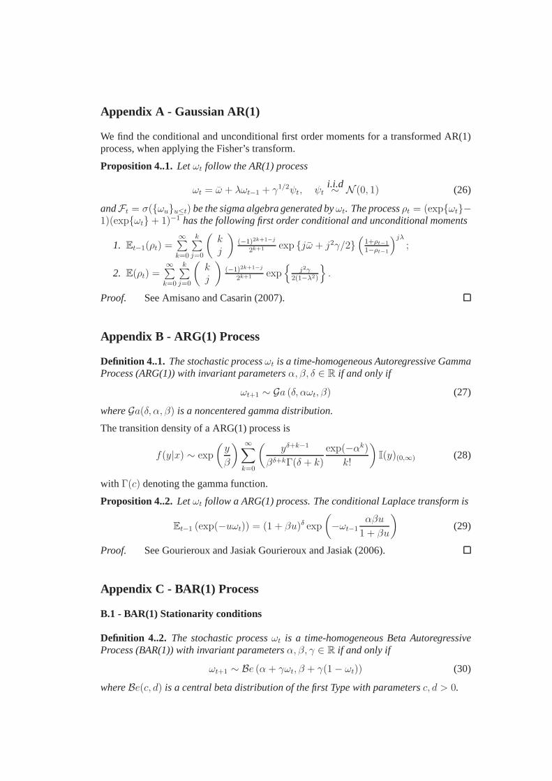
Appendix A - Gaussian AR(1)

We find the conditional and unconditional first order momentsfor a transformed AR(1)process, when applying the Fisher’s transform.

Proposition 4..1. Letωt follow the AR(1) process

ωt = ω + λωt−1 + γ1/2ψt, ψti.i.d∼ N (0, 1) (26)

andFt = σ(ωuu≤t) be the sigma algebra generated byωt. The processρt = (expωt−1)(expωt + 1)−1 has the following first order conditional and unconditionalmoments

1. Et−1(ρt) =∞∑

k=0

k∑

j=0

(

kj

)

(−1)2k+1−j

2k+1 exp jω + j2γ/2(

1+ρt−1

1−ρt−1

)jλ

;

2. E(ρt) =∞∑

k=0

k∑

j=0

(

kj

)

(−1)2k+1−j

2k+1 exp

j2γ2(1−λ2)

.

Proof. See Amisano and Casarin (2007).

Appendix B - ARG(1) Process

Definition 4..1. The stochastic processωt is a time-homogeneous Autoregressive GammaProcess (ARG(1)) with invariant parametersα, β, δ ∈ R if and only if

ωt+1 ∼ Ga (δ, αωt, β) (27)

whereGa(δ, α, β) is a noncentered gamma distribution.

The transition density of a ARG(1) process is

f(y|x) ∼ exp

(

y

β

) ∞∑

k=0

(

yδ+k−1

βδ+kΓ(δ + k)

exp(−αk)

k!

)

I(y)(0,∞) (28)

with Γ(c) denoting the gamma function.

Proposition 4..2. Letωt follow a ARG(1) process. The conditional Laplace transformis

Et−1 (exp(−uωt)) = (1 + βu)δ exp

(

−ωt−1αβu

1 + βu

)

(29)

Proof. See Gourieroux and Jasiak Gourieroux and Jasiak (2006).

Appendix C - BAR(1) Process

B.1 - BAR(1) Stationarity conditions

Definition 4..2. The stochastic processωt is a time-homogeneous Beta AutoregressiveProcess (BAR(1)) with invariant parametersα, β, γ ∈ R if and only if

ωt+1 ∼ Be (α + γωt, β + γ(1 − ωt)) (30)

whereBe(c, d) is a central beta distribution of the first Type with parameters c, d > 0.

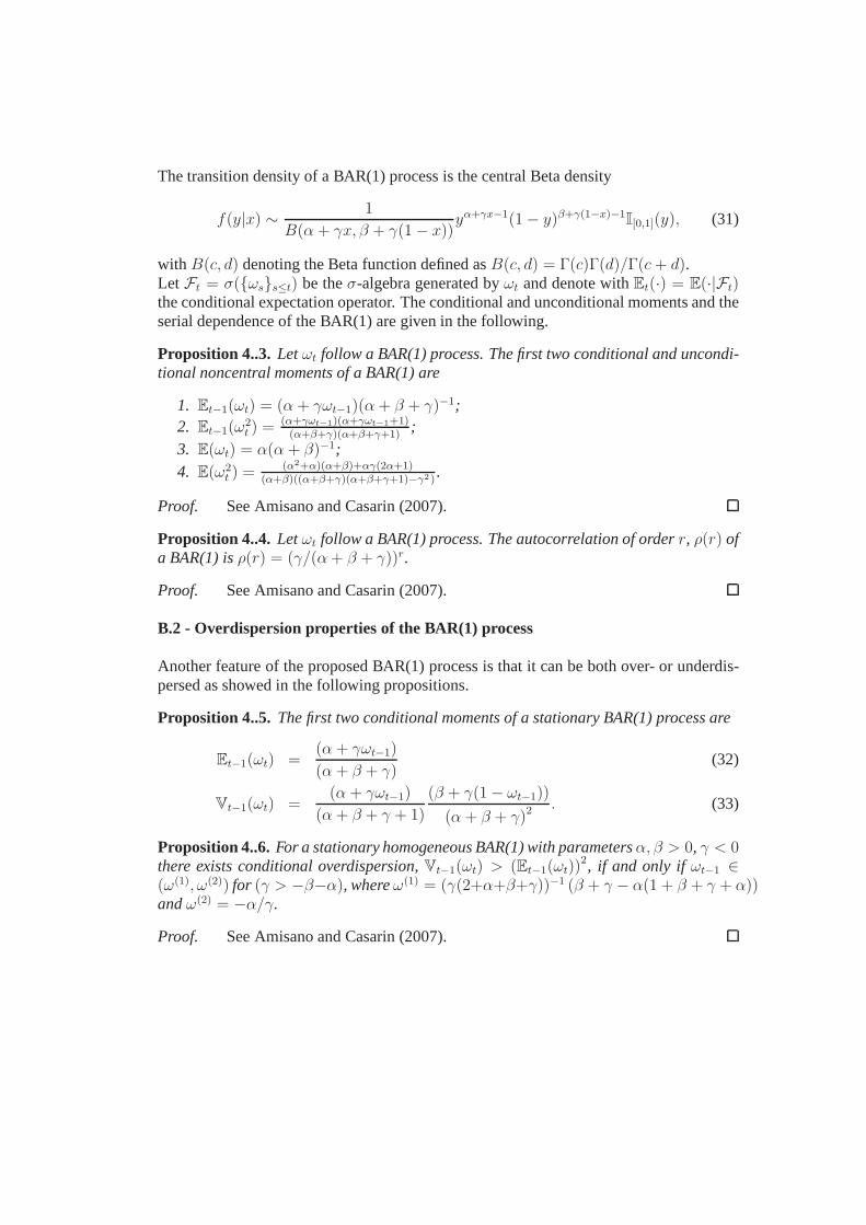
The transition density of a BAR(1) process is the central Beta density

f(y|x) ∼1

B(α + γx, β + γ(1 − x))yα+γx−1(1 − y)β+γ(1−x)−1

I[0,1](y), (31)

with B(c, d) denoting the Beta function defined asB(c, d) = Γ(c)Γ(d)/Γ(c+ d).Let Ft = σ(ωss≤t) be theσ-algebra generated byωt and denote withEt(·) = E(·|Ft)the conditional expectation operator. The conditional andunconditional moments and theserial dependence of the BAR(1) are given in the following.

Proposition 4..3.Letωt follow a BAR(1) process. The first two conditional and uncondi-tional noncentral moments of a BAR(1) are

1. Et−1(ωt) = (α + γωt−1)(α+ β + γ)−1;2. Et−1(ω

2t ) = (α+γωt−1)(α+γωt−1+1)

(α+β+γ)(α+β+γ+1);

3. E(ωt) = α(α + β)−1;

4. E(ω2t ) = (α2+α)(α+β)+αγ(2α+1)

(α+β)((α+β+γ)(α+β+γ+1)−γ2 ).

Proof. See Amisano and Casarin (2007).

Proposition 4..4.Letωt follow a BAR(1) process. The autocorrelation of orderr, ρ(r) ofa BAR(1) isρ(r) = (γ/(α+ β + γ))r.

Proof. See Amisano and Casarin (2007).

B.2 - Overdispersion properties of the BAR(1) process

Another feature of the proposed BAR(1) process is that it canbe both over- or underdis-persed as showed in the following propositions.

Proposition 4..5. The first two conditional moments of a stationary BAR(1) process are

Et−1(ωt) =(α + γωt−1)

(α + β + γ)(32)

Vt−1(ωt) =(α + γωt−1)

(α + β + γ + 1)

(β + γ(1 − ωt−1))

(α + β + γ)2 . (33)

Proposition 4..6.For a stationary homogeneous BAR(1) with parametersα, β > 0, γ < 0there exists conditional overdispersion,Vt−1(ωt) > (Et−1(ωt))

2, if and only ifωt−1 ∈(ω(1), ω(2)) for (γ > −β−α), whereω(1) = (γ(2+α+β+γ))−1 (β + γ − α(1 + β + γ + α))andω(2) = −α/γ.

Proof. See Amisano and Casarin (2007).