Classical Estimation of MultivariateMarkov-Switching Models using MSVARlib

Benoıt Bellone 1

This version - July 2005(First draft - February 2005)

Abstract

This paper introduces an upgraded version of MSVARlib, a Gauss and Ox-Gausscompliant library, focusing on Multivariate Markov Switching Regressions in theirmost general specification. This new set of procedures allows to estimate, throughclassical optimization methods, models belonging to the MSI(M)(AH)-VARX “inter-cept regime dependent” family. This research enhances the first package MSVARlib1.1, which has been deeply inspired by the works of Hamilton and Krolzig. Not tomention the extension to a generalized multivariate regression framework, it notablyaugments the range of models with a possibly unlimited finite number of Markovstates, offers automatic or manual intialization procedures and adds new statisticaltests. The first part of this article provides the basic theoretical grounds of therelated Markov-switching models. Following sections give some illustrations of theprograms through univariate and multivariate examples. One is based on a non-linear reading of the american unemployment rate. A second study is focused oncoincident stochastic models of US recessions and slowdowns. The paper concludeson possible extensions and new applications. Detailed guidelines in appendices andtutorial programs are provided to help the reader handling the Gauss package andthe joined replication files.

Key Word: Multivariate Markov-Switching Regressions, Hidden markov Models,Open source Gauss library, Business cycle, EM algorithm, Kittagawa-Hamilton Fil-teringJEL Classification: C32, E32, E44

The views expressed in this working paper are those of the author and do not repre-sent those of the OECD. This article describes personal research in progress by theauthor and is published to elicit comments, to further debate and call for materialcollaboration in future developments of this library.

1Corresponding author. OCDE, 2, rue Andre Pascal 75016 Paris, tel: (33)1 45 24 95 18. E-mailaddress: benoit.bellone (at) ensae.org.

1 Introduction.

MSVARlib 2.0, Markov-Switching Vector Autoregression Library, is an upgraded open-source basic package designed to model univariate or multivariate regime dependenttime series. Among the available public resources in matrix languages, lots of programshave spread thanks to the work of Kim and Nelson (1999) and Hamilton (1989), howevermost of their routines were not designed in a general multivariate framework, but ratheras specific programs not so easy to be extended.

Econometricians or statisticians may be eager to understand their estimate resultsand to master all the assumptions and implied choices related to the numerical proce-dures inside their programs. MSVARlib has been designed on this purpose: it offers anopen-source set of procedures dedicated to estimate basic mixing law models inspiredby Hamilton (1994) or generic Multivariate Markov-Switching regressions. Providinga wider array of specifications regarding autoregressive and exogenous systems, it isfully related to the MSVAR library developed by Krolzig (1998)2 focusing on Markov-Switching Vector Autoregressions estimates through maximum likelihood methods. Tomy knowledge, there are few libraries covering the extent of the MSVARlib package.The Krolzig’s MSVAR library offers a comprehensive and integrated toolbox, with lotsof diagnostic tools3. However it is not available on a free access and on an open-sourcebasis4. Khaled (2004), has also developped a promising Matlab package following aBayesian approach and covering the same kind of specifications, but is not public forthe time being.

Contrary to Ox, the library is not designed in an oriented-object environment, butstill fully uses the power of a matrix language. It has been first developed in the Gaussenvironment, to propose a flexible way for applied economists to estimate hidden markovmodels in a familiar and widespread language matrix. However the use of specific gausssubroutines and matrix operators has been minimized so as the library to be easilytranslated in other languages. Thus, this package is being developed in the Scilabenvironment and might eventually be included in the GROCER Toolbox, a completeeconometric package designed by Eric Dubois5.

The paper is organized as follows. The first two sections introduce and deliver theusual copyright and disclaimers. The third section presents the general framework ofMultivariate Markov-Switching Regression Models covered by the library and discussesits derivative models. The fourth sections hints at log-likelihood and related algorithms.The fifth section gives some illustrations through univariate and multivariate estima-tions. It introduces a stochastic model of the American unemployment rate and hintsat two US-coincident business cycle models, already outlined in Ferrara (2003), Bellone,Gautier and Lecoent (2004) or Bellone (2004a). The fifth section concludes on possibleextensions to co-integrated models and enhanced diagnosis tools. Detailed guidelines in

2Because they have inspired this research a lot, a careful reading of Krolzig’s and Doornik’sworks should be all the more useful. See http://www.economics.ox.ac.uk/research/hendry/krolzig/ andhttp://www.doornik.com/index.html.

3In this respect, MSVAlib 2.0 has been quite enhanced compared to the primal version 1.1 introducedin Bellone (2004b), but remains more modest.

4MVAR is a compiled, proprietary package.5Grocer is availabe at http://dubois.ensae.net/ and is referenced as a contribution on the Scilab web

site http://scilabsoft.inria.fr/

2

appendices are provided to help the reader handling the MSVARlib Gauss package andits related replication files.

2 Copyright, Conditions of Use and Disclaimer.

The GAUSS programs available on the website http://bellone.ensae.net6 are writtenand copyrighted c© 2004 by Benoit BELLONE, all rights reserved. They can be run onGauss 3.2 or upper versions and should be OX-Gauss compliant, thanks to the routineM@ximize developped by Laurent and Urbain (2005)7. The code is licensed gratis to allthird parties under the terms of this paragraph. Copying and distribution of the filesin this archive is unrestricted if and only if the files are not modified. Modification ofthe files is encouraged, but the distribution of modifications of the code in this archiveis unrestricted only if you meet the following conditions: modified files must carry aprominent notice stating

(i) the original author and date,

(ii) the new author and the date of release of the modification,

(iii) that there is no warrantee for the code, and

(iv) that the work is licensed at no charge to all parties.

If you use the code extensively in your research, you are requested to provide appropriateattribution and thanks to the author of the code. No representation is made or impliedas to the accuracy or completeness of the programs which may indeed contain bugs orerrors unknown to the author. Benoit Bellone takes no responsibility for results producedby MSVARlib programs which are used entirely at the reader’s risk. This package is byno means finished yet, a enhancement “to do list” remains open. If you plan to extendthe library, find any problems or have suggestions for improvement, contact the author8.

3 The general multivariate Markov-switching regressionmodel and its derivatives.

For a comprehensive presentation of Markov-Switching Vector Auto-Regression models,the reader should first report to Krolzig (1997) and to Krolzig (1998) or Krolzig (2003)for a complete introduction to the estimations of regime switching models with Ox. Thelibrary owes also a lot to the previous works of Roncalli (1995) who developped manyeconometric routines in Gauss that were heavily used or transformed in this package.For a basic presentation of Hidden Markov Models and simple gaussian distribution mix-tures, one should report to Hamilton (1994). Note that contrary to MSVARlib 1.1, the2.0 version of the library covers an extended range of models. Following the Krolzig tax-onomy, this version includes the MSI(M)(AH)-VARX(q) “intercept regime dependent”

6Also on the mirror site http://perso.magic.fr/benbellone7This Ox package is an Optmum substitute for Ox users and is available at

http://www.core.ucl.ac.be:16080/ laurent, Sebastien Laurent’s web site.8Email: benoit.bellone (at) ensae.org

3

family, but excludes the MSM(M)-VARX(q)“mean regime dependent” models. Thisversion introduces a generic open source code and functions, that should be easy toextend to more complex specifications such as co-integrated Markov-Switching Modelsor regime dependent volatility models.

3.1 A general multivariate Markov-Switching framework.

Be yt = (y1,t, . . . , yp,t) a vector of size (1, p), with p the number of variables of interest.We define St = {1 . . .M} as a M-state unobserved variable, following a first orderMarkov Chain. St = 1 (resp. St = M), means that the time series are said to be inthe “lowest” (resp. the “highest”) regime. The matrix P of transition probabilities isdefined very classically, following notations in Hamilton (1994):

P =

p11 . . . pM1

p12 . . . pM2...

......

p1M . . . pMM

, withM∑

j=1

pkj = 1, and, pkj > 0, ∀k, j ∈ {1 . . .M}.

Let It−1 = (yt−1, . . . , y1), the information set available in t-1, then :

pkj = P (St = j|St−1 = k, . . . , S1 = l, It−1)= P (St = j|St−1 = k), ∀k, j ∈ {1 . . .M}.

The “shadow random variable”9 ξt denotes a (M, 1) vector whose jth element is definedas follows, ∀j ∈ {1 . . .M}:

ξjt = ISt=j , and, ξt =

(ξ1t . . . ξM

t

).

When St = j, then ξt = e′j where ej is the jth column vector of the identity matrix IM ,which leads to :

ξt =M∑

j=1

e′j .ξjt .

Thanks to these notations, the conditional probability related to the state j is expressedas:

P (St = j|It) = E(ξjt |It)

and we note the vector of filtered probabilities:

P (St|It) = E(ξt|It) =(

P (St = 1|It) . . . P (St = M |It))

= ξt/t =(

E(ξ1t |It) . . . E(ξM

t |It)).

Let xt = (x1,t, . . . , xn,t) and zt = (z1,t, . . . , zq,t) be (1, n) (resp. (1, q)) vectors ofexogenous regressors subject (resp. not subject) to switching regimes. We note respec-tively βSt = (β1

St, . . . , βp

St) the (n, p) matrix of regression-coefficients which are regime

dependent, and δ = (δ1, . . . , δp) the (q, p) matrix of regression-coefficients which areregime independent. Let 1p be a (1, p) vector of 1’s and define:

ΓSt = (βSt |δ)′ and, At = (xt|zt)9See Hamilton (1994), pp 679.

4

The most general model estimated with MSVARlib is a Markov Switching GaussianModel : {

yt = At.ΓSt + ut

ut|St ∼ N(0,ΣSt)

with

ΣSt =

σ11(St) . . . σ1M (St)...

. . ....

σM1(St) . . . σMM (St)

such as 10,

σii(St) = σ2i (St), σii(St) > 0

σij(St) = ρij(St).σi(St).σj(St), ∀i 6= j ∈ {1..M}.

Differencing independent and dependent regime regressors, we introduce the equiv-alent formula11: {

yt = xt.βSt + zt.δ + ut

ut|St ∼ N(0,Σst)(1)

MSVARlib allows different specifications of regime dependent (resp. independent)covariance matrix such as :

• Generalized Covariance Matrix:

ΣSt = (σij(St)) or, Σ = (σij), ∀i, j ∈ {1..M}

• Heteroskedastic Covariance Matrix:

ΣSt =

σ21(St) . . . 0

0. . . 0

0 . . . σ2M (St)

or, ΣSt = Σ =

σ21 . . . 0

0. . . 0

0 . . . σ2M

• Homoskedastic Covariance Matrix:

ΣSt = σ2(St).Ip or, Σ = σ2.Ip.

3.2 MSVARlib and its derivative models.

MSVARlib offers five different family models12, that are a derived form of the equation(1):

(1) The Mean-Variance model:

yt = νSt + ut = 1p.βSt + ut, (2)

10The following representation is all the more important as it is used to constraint the parameters,see MSVARinit.prg.

11In fact, it corresponds to the Model 4, see further.12Those models are related to the option typmod, taking the value 1 to 5 in the program

5

(2) The MS-VAR regime dependent model:

yt = νSt + yt−1.β1St

+ · · ·+ yt−q.βqSt

+ ut = (1p, yt−1, . . . , yt−q).βSt + ut, (3)

(3) The MS-VAR Intercept regime dependent model:

yt = νSt + yt−1.δ1 + · · ·+ yt−q.δq + ut = 1p.βSt + (yt−1, . . . , yt−q).δ + ut (4)

(4) The partially regime dependent MS-Regression model:

yt = xt.βSt + zt.δ + ut, (5)

(5) The general MS-Regression model:

yt = xt.βSt + ut, (6)

The first specification corresponds to the simpler version MSI(M)H-VAR(0) model whichis used in Ferrara (2003) or Bellone (2004a) to extract a US-recession model. Followingthe Krolzig taxonomy, the Model 2 (resp. Model 3) can be identified as a MS(M)-VAR(q) (resp MSI(M)-VAR(q)) model. Eventually, both “Markov-switching” multi-variate regressions are implemented via “mix” models with partial (Model 4) or fullregime dependency (Model 5), which are close to MSI(M)-VARX Krolzig’s modelling.Of course, each specification can be combined to different covariance options, as men-tioned in the previous section.

4 The Log-Likelihood, the Filters and the EM algortihm

4.1 A conditional innovation gaussian model.

From a practical point of view there are M “shadow models”, which are piled up duringthe estimates with:

ΣSt = Σ1ξ1t + · · ·+ ΣMξM

t and, βSt = β1ξ1t + · · ·+ βMξM

t .

So, M distinct models are simultaneously estimated such as:

(1p ⊗ yt) = xt.(β1| . . . |βM ) + (1p ⊗ zt).δ + (u1t | . . . |uM

t ).

Conditioning by St, M different (p × 1) gaussian vectors have to be taken intoaccount. Thus, for a given regime St = j:{

yt = xt.βj + zt.δ + ut

ut|St = j ∼ N(0,Σj)(7)

Let’s note µt,j = xt.βj + zt.δ and let Θ be the (1, nΘ) vector of related parameters.Then, the conditional probability density function is:

f(yt|St = j, It−1,Θ) = (2π)−p2 .det(Σ

− 12

j ).exp(−

(yt − µt,j)′Σ−1j (yt − µt,j)2

). (8)

6

To a certain extent, the models can then be summed-up as a M “stacked” vector of condi-tional gaussian densities estimated by maximum likelihood with the following propertieslinked to the Kitagawa-Hamilton filter. To summarize the logic of the MSVAR mainprogram:

• First, initial values of the vector of parameters are calculated. If the automaticintializer is choosen , the series are sorted, split in M parts on which initial con-ditional regressions are computed to launch the Maximum likelihood descent. Ifavailable, an initial a priori datation can be loaded and use to sort the data.Eventually, manual initialization remains possible, whether in practice, not oftenused.

• Second, the model is recursively estimated through the “EM” algorithm, startingfrom the unconditional density of yt which is calculated by summing conditionaldensities over possible values for St:

f(yt|It−1,Θ) =M∑

j=1

P (St = j, yt|It−1,Θ)

or,

f(yt|It−1,Θ) =M∑

j=1

P (St = j|It−1,Θ).f(yt|St = j, It−1,Θ). (9)

The maximum likelihood estimate of Θ is obtained by maximizing the log-likelihood :

L(Θ) =T∑

t=1

ln(f(yt|It−1,Θ))

with Θ = (θP , θβ , θδ), θΣ), is the vectorized matrix of parameters13.

4.2 A priori filtering and smoothing with the Kittagawa-Hamilton’salgorithms.

The filtered probability is computed such as:

P (St = j|It,Θ) = P (St = j|yt, It−1,Θ) =P (St = j, yt|It−1,Θ)

f(yt|It−1,Θ)

that is to say:

P (St = j|It,Θ) =P (St = j|It−1,Θ).f(yt|St = j, It−1,Θ)∑M

k=1 P (St = k|It−1,Θ).f(yt|St = k, It−1,Θ)(10)

Following the notations of Krolzig or Hamilton, the algorithm replicates the genericfollowing formula to extract a M ×T matrix of filtered probabilities, the components ofwhich are expressed in the following matrix:

13MSVAR init.prg should be carefully examined to master all the details related to the constrainedoptimization and initialization of parameters.

7

P (St|It) = ξt/t =f(yt|St)� ξt/t−1

1′M(f(yt|St)� ξt/t−1

) (11)

where � (.* in the Gauss matrix language) designates the element by element product.A novel aspect of the MSVARlib package is also to define a more concise formulationof the smoothing algorithm in a multivariate specification, that of course applies in anunivariate framework through the recursive formula:

P (St|IT ) =(P (St|It)′ �

{P ′ [P (St+1|IT )′ � P (St+1|It)′

]} )′, ∀t ∈ {1 . . . T − 1} (12)

where � (./ in the Gauss matrix language) designates the element by element division.For a more comprehensive cover of the Baum-Lindgren-Hamilton-Kim (BLHK) filtersand smoothers in a multivariate framework, the reader should report to Krolzig(1997),chap 5, and Hamilton (1994), chap 22.

5 Three illustrations of MSVARlib estimations.

Many replication files are joined with the MSVARlib package. Here we propose to detailan univariate models MSI(2)-AR(q) and two multi state multivariate Mean-Variancemodel(MS(M)-VAR(0)) which refer to some illustrations of Ferrara (2003), Bellone,Gautier, Lecoent (2004) and Bellone (2004a).

5.1 A stochastic MSI(2)-AR(q) analysis of the US employment rate

In the program UNMod3.prg and UNMod1.prg, we assume that the dynamic of the USunemployment rate14 is subject to two regimes: a low one identifying a steep rise inunemployment and a high regime, matching a stabilization or a decrease in the unem-ployment rate. Many papers, see for instance Rothman (1998) or Hamilton (2005) for ajustification of such a model by asymmetric variations during NBER recessions callingfor possible non-linear behaviors.

If we note y∗t the reverse two-month growth rate of unemployment (ie y∗t = 100 ×(ln(unt−2)− ln(unt)), with unt the US unemployment rate, and yt the related standard-ized growth rate.

The model MSI(2)H-AR(3) is summarized as follow:{yt = νSt + δ1.yt−1 + δ2.yt−2 + δ3.yt−3 + ut

ut|St ∼ N(0, σ2St

) with, St ∈ {1, 2}. (13)

The model MSI(2)H-AR(0) is a simple Mean-Variance model:{yt = νSt + ut

ut|St ∼ N(0, σ2St

) with, St ∈ {1, 2}. (14)

14Here we deal with 1/ut to match a rise in the probability of being in a low regim with a rise in theunemployment rate

8

Here, intercepts and variance are regime dependent:

νSt = ν1ξ1t + ν2ξ

2t , with ν1 < ν2 and, σ2

St= σ2

1ξ1t + σ2

2ξ2t .

2

3

4

5

6

7

8

9

10

11

12

1967

1969

1971

1973

1975

1977

1979

1981

1983

1985

1987

1989

1991

1993

1995

1997

1999

2001

2003

Une

mpl

oym

ent r

ate

as

a %

of l

abor

forc

e

0.0

0.1

0.2

0.3

0.4

0.5

0.6

0.7

0.8

0.9

1.0

Smoo

thed

pro

babi

lity

of lo

w re

gim

e

Datation NBER MSI(2)H-AR(3)

Figure 1: Smoothed probability of the MSI(2)-AR(3) low regime - Unemployment ratemodel

Appendix B (page 18) provides the detailed estimated parameters, standard devia-tions, transformed parameters, normality test on residuals, information criteria , graphsof filtered and smoothed probabilities and graphs of residuals . Figure 1 shows theorginal unemployement series, the NBER datation and the smoothed probabilities ofcontracting. The hypothesis of normality of residuals cannot be rejected in the specifi-cation of the first model, contrary to the simpler mean-variance model. However, if thisspecification is not statistically rejected, autoregressive components are often quite sub-ject to critics. If they correct for non-gaussian disturbances, they might deteriorate thequality of the signal of the filtered probability. Thus, it should be noted that (see Figure2) the more parcimonious model sends far clearer and even earlier signals of turningpoint, as already noticed by Albert and Chib (1993) and Lahiri and Wang (1994).

To conclude this section, as mentioned in Anas and Ferrara (2002) or in Bellone andSaint-Martin (2003), the unemployment rate remains one of the most reliable coinci-dent indicator to detect recessions and confirm some non linear behavior. Appendix Cestimates and graphs give some evidence of the following stylized facts : accelerationsare steep in recession (the average standardized growth rate of rising unemployment isfourfold the average standardized growth rate of decrease in unemployment), decreasesare slow in recovery phase, volatility is higher in recessionary phases (the variance ofthe low regime is twofold the high regimes’ one).

9

0

0.1

0.2

0.3

0.4

0.5

0.6

0.7

0.8

0.9

1

1967

1968

1969

1970

1971

1972

1973

1974

1975

1976

1977

1978

1979

1980

1981

1982

1983

1984

1985

1986

1987

1988

1989

1990

1991

1992

1993

1994

1995

1996

1997

1998

1999

2000

2001

2002

Filt

ered

pro

babi

lity

of re

cess

ion

AR(3) AR(0)

Figure 2: Filtered probabilities of the MSI(2)-AR(3) and MSI(2)-AR(0) low regime -Unemployment rate model

5.2 Detecting US recessions and slowdowns with Markov-Switchingmodels.

Two stochastic models of the US business cycles are presented in this section. First amodel estimated by Bellone (2004a) with the assumption of two regimes “recession vsexpansion”. A more refined model is estimated, extending the assumptions of Ferrara(2003) by Bellone, Gautier, Lecoent (2004), which introduce a third regime. The firstmodel includes four series in the following order: the reversed unemployment rate, thehelp wanted advertising index, the Industrial Production index, 1000/Jobs hard to Getcomponent (see the MSVARRec4.txt file and the MSVAR.prg program). Bellone (2004a)prefers a two-state model rather than a three-state model because of higher stabilityand robustness to changes in an extended sampling period of 1967-2000. The relatedmodel is a MS(2)H-VAR(0) :{

(y1,t, . . . , y4,t) = (ν1,St , . . . , ν4,St) + ut

ut|St = (u1,t, . . . , u4,t)|St ∼ N(0,ΣSt)(15)

with,

St ∈ {1, 2} and ΣSt =

σ21(St) . . . σM1(St)

.... . .

...σ1M (St) . . . σ2

M (St)

The figure 3 gives evidence that each period of a low regime of the filtered probability

is coincident with a NBER recession. As expected, covariances in the lower regime arebigger than in the “growth” regimes. Note that the seven NBER recessions are clearly

10

0

0.1

0.2

0.3

0.4

0.5

0.6

0.7

0.8

0.9

119

6719

6819

6919

7019

7119

7219

7319

7419

7519

7619

7719

7819

7919

8019

8119

8219

8319

8419

8519

8619

8719

8819

8919

9019

9119

9219

9319

9419

9519

9619

9719

9819

9920

0020

0120

02

Filte

red

prob

abili

ty o

f rec

essi

on

0

0.1

0.2

0.3

0.4

0.5

0.6

0.7

0.8

0.9

1

Datation NBER MRec4 MSI(2)-VAR(0)

Figure 3: US coincident multivariate model - Filtered probability of a recession.

detected with the “low regime” filtered probability, with short lags: over the eightiespeaks are detected on average with one month lags, and trough are coincident. Becausethree series out of four are un-revised on a short term basis, this indicator should deliverreliable and timely real-time signals of start and end of a recession. The reader can referto Bellone (2004a) for the estimations or use the MSVAR.prg program to replicate thoseresults15.

Figure 4 echoes a really close model as introduced in equation (15). IT differs onlyby the number of regimes: St ∈ {1, 2, 3} and by an assumption of regime independencyof covariance: Σ(St) = Σ, following Ferrara (2003) and some statistical tests. It is anenhanced estimation of the model proposed by Ferrara (2003): three filtered probabilitiesare calculated, associated to three states : “low growth ”, “medium or below potential” and “high growth ”. To sum this in two signals, the difference of high and low regimeprobabilities is calculated (bold line), varying between −1 and 1, and the intermediateregime is directly represented by the associated filtered probability. The slowdownperiods are signaled by a rising medium regime probability , varying between 0 and −1,that is a drop of the dashed line in negative territory or by oscillations of the differenceof filtered probabilities around 0 (see “High-Low” bold line ). Recessions are signaledby a significant drop 16 in negative territory, and steady growth by a probability in apositive territory. This three-state model is implemented in the Model1.prg program,

15The Mrec4 model is selected as the reference model in MSVAR.prg16Usually with a probability above 50%.

11

full detailed results, of which transition matrix, parameters and ergodic probabilities,related standard deviations are printed out in the Threestate\_output.txt and a shortsummary is printed in Appendix C page 23. This model deals with the first three seriespreviously mentioned and adds real construction spending 17.

-1

-0.8

-0.6

-0.4

-0.2

0

0.2

0.4

0.6

0.8

1

2.19

84

2.19

85

2.19

86

2.19

87

2.19

88

2.19

89

2.19

90

2.19

91

2.19

92

2.19

93

2.19

94

2.19

95

2.19

96

2.19

97

2.19

98

2.19

99

2.20

00

2.20

01

2.20

02

Filte

red

prob

abili

ties

and

diffe

renc

e of

filte

red

prob

abili

ties

NBER Datation High - Low Medium

Figure 4: Filtered probabilities of the Three state model. Estimation period (1984-1 /2003-2)

As introduced by Lahiri and Wang (1994) or Sichel (1994) three state-models mayoffer a more precise description of short term macroeconomic developments, exhibitingalternance of high growth, slow growth and recession regimes. The three-state modelsallows to detect “slowdowns”, often early warning of a recessionary period, such as thoseobserved in 1989 or in early 2000. It also hints at the qualitative intensity of a recoveryor a slowdown in the business cycle as in early 1992 or in early 2003. However, the modelseems extremely sensitive to the sampling period, which denotes a likely low robustnessbefore 1984 and a lack of stability (or identification abilities) between the medium andthe high regime18. The reader should experience varying estimation periods, differentoptions of covariance matrix specification and a test of a MSI(M)H-VAR(q) extensionto judge this effective sensitivity compared to a two-state specification.

17Since 2004, the BLS has stopped producing those series. New releases starts only at the beginningof the 90’s. Besides, because of a less timely publication and those disrupted samples, Bellone (2004a)discarded the construction spending series and included a survey dealing with employment condition,the “Jobs hard to get” component.

18This is a well known feature of the US business cycle, studied in detail by Stock and Watson (2003)and discussed also in Bellone, Gautier, Lecoent (2004)

12

6 Conclusion.

MSVARlib should provide to the applied econometrician convenient and open sourceprograms to estimate through EM algorithm basic and generic Multivariate MarkovSwitching Regression models. MSVARlib is still a modest package and a less ”userfriendly”’ than the Krolzig’s “MSVAR for Ox” compiled programs, but the package istransparent, quite flexible and could be easily adapted to new inclusive models such asMarkov switching volatility models, Short-term forecasts automatic models... If a “todo list” had to be designed, here could be the next adds and improvement:

• a clearing and optimization of algorithms (there are probably some gains to make),

• an extension of the model to “Student” innovations to challenge the gaussianassumption, as proposed in Hamilton (2005),

• a development of news statistical tests and tools which would complete the newpackages introduced in the 2.0 version (information criteria, normality tests...)such as correlograms, spectral densities, empirical densities, Davies Test, specifi-cation tests of Hamilton (1996) or Carrasco et al.(2004), and non-linearity testssuch as the one proposed in Hansen (1992). . . ,

• an extension to forecasting and co-integration analysis,

• an adaptation to a Multivariate Bayesian approach with a Multimove Gibbs sam-pler as proposed in Khaled (2004).

Acknowledgements.

I am grateful to Vladimir Borgy and David Saint-Martin for their material helpduring the first stages of this research, to Eric Dubois and Emmanuel Michaux fortheir support, to Erwan Gautier and Sebastien Laurent for their careful debugging ofnever-ending new versions. I also would especially like to thank Fabrice Lenglart whostimulated most of this work and gave me access to lots of resources.

13

References

Albert, J H., Chib, S. (1993), Bayes Inference via Gibbs Sampling of Autoregressive TimeSeries Subject to Markov Mean and Variance Shifts, Journal of Business and Economic Statistics,11, pp. 1-15.

Anas, J., Ferrara, L. (2002), Un indicateur d’entree et de sortie de recession: application auxEtats-Unis, Centre d’Observation Economique, Paris, Working paper.

Andersson, E., Bock, D., Frisen, M. (2002), Detecting of Turning Points In Business Cycles,26th CIRET Conference, Taipei , Working paper.

Bellone B., Saint-Martin D. (2003), Detecting Turning Points with Many Predictors throughHidden Markov Models, Working paper, Seminaire Fourgeaud, 3 decembre 2003.

Bellone B. (2004a), Une lecture probabiliste du cycle d’affaires americain, April 2004, revisedFebruary 2005, Working paper, http://bellone.ensae.net.

Bellone B. (2004b), MSVARlib : a new Gauss Library to Estimate Multivariate Hidden MarkovModels, Working paper and Gauss library available at http://bellone.ensae.net.

Bellone B., Gautier E., Lecoent S. (2004), Les marches financiers anticipent-ils les re-tournements conjoncturels?, June 2004, revised February 2005, Working paper.

Carrasco M., Liang H., Ploberger W. (2004), Optimal Test for Markov Switching, Workingpaper, University of Rochester.

Dubois, E. (2004), GROCER 1.0 : An Econometric Toolbox for Scilab: an EconometricianPoint of View, Working paper.

Ferrara, L. (2003), A Three-Regime Real-Time Indicator for the US Economy, EconomicsLetters, Vol. 80, n 3, pp. 373-378.

Hamilton, J.D. (1989), A new Approach to the Economic Analysis of Nonstationary TimeSeries and the Business Cycle , Econometrica, vol.57, No 2 pp. 357-384.

Hamilton, J.D. (1994), Time Series Analysis, Princeton University Press ed, Chap 22, pp677-703.

Hamilton, J.D. (1996), Specification Testing in Markov-Switching Time Series Models, Journalof Econometrics, 70, pp. 127-157.

Hamilton, J.D. (2005), What’s Real About the Business Cycle?, NBER Working Paper, w11161.

Hansen, B.E. (1992), Testing for Parameter Instability in Linear Models, Journal of PolicyModeling, 14, 4, pp. 517-533.

Khaled, M. (2004), Multivariate Markov Switching Regressions, Working paper.

Kim, C. J., Nelson, C. R. (1999), State-Space Models with Regime Switching, MIT Press ed.

Krolzig, H. M. (1997), Markov Switching Vector Autoregressions. Modelling Statistical Infer-ence and Application to Business Cycle Analysis, Springer Verlag ed.

Krolzig, H. M. (1998), Econometric Modelling of Markov-Switching Vector Autoregressionsusing MSVAR for Ox, Working paper.

Krolzig, H. M. (2003), Constructing Turning Point Chronologies with Markov-Switching VectorAutoregressive Models: the Euro-Zone Business Cycle, Working paper.

Lahiri, K., Whang J. G. (1994), Predicting Cyclical Turning Points with leading index in theMarkov Switching model., Journal of Forecasting, vol. 13, pp. 245-263.

Laurent, S., Urbain J. P. (2005), Bridging the Gap between Gauss and Ox using OXGAUSS,Journal of Applied Econometrics, vol. 20,1, pp 131-139.

Roncalli, T. (1995), Introduction a la programmation sous GAUSS, Applications a la Financeet a l’Econometrie, vol 2, Ritme informatique ed.

14

Rothman, P. (1998), Forecasting Asymmetric Unemployment Rates, The Review of Economicsand Statistics, 80, pp.164-168.

Sichel, E. D. (1994), Inventories and the Three Phases of the Business Cycle, Journal ofBusiness and Economic Statistics, Vol 12, No 3, pp. 269-277.

Stock J.H., Watson M.W. (2003), Has the Business Cycle changed? Evidence and expla-nations, forthcoming FRB Kansas City symposium, Jackson Hole, Wyoming, August 28-30,2003.

15

Appendix A :Installation and Main structures

Before installing the package and execute the applications, you need to be able to run a GAUSSprogram. For the time being, MSVARlib 2.0 is written in the GAUSS R© matrix language andrequires the GAUSS R© 3.2 or a later version of the software. It has been tested on the 3.2, 5.0and 6.0 versions and has been designed in a WINDOWS 95/NT environment. It should be soonextended in the Scilab language.

To install and run these programs, you must absolutely create a directory C:\GAUSS\MSVARwhere you should unzip the MSVARlib package. This package includes two directories, a readmefile and this paper:

- the MSLIB directory includes the main program MSVAR.prg, program files and saved outputresults, - the DATA directory includes input data files and data sample spreadsheets with conve-nient templates. - Readme.txt exhibits those basic installation instructions - the MSLIB\EXAMPLESincludes example program files related to this paper.

Once unzipped, you should place the first two directories in the following subdirectories:

C:\GAUSS\MSVAR\MSLIBC:\GAUSS\MSVAR\DATA

To start theestimation, open the Gauss R© program, select C:\GAUSS\MSVAR\MSLIB as yourworking library.

Data organization

In the DATA directory, some sample files are available. They are all ASCII files, saved in the$\text{".txt"}$ format with tab-spaces separators. These data are based upon Americansurveys and quantitative time series starting from January 1960, an depending on the vintage,to February 2004 or February 2003. The first two columns of an input file should start with amonth series (m format: 1 to 12) and a year series (yyyy format), the following columns shouldrefer to data. No label should be referenced A missing value is represented by a dot ”.”.

Here is a list of included sample files in the DATA directory:

• MSVARrec4.txt includes the four series used in Bellone (2004b) as a US recession twostates hidden markov models: they belong to the ”April 2004 vintage” (february 2004 isthe minimal common date). Those four series are: the reversed unemployment rate, thehelp wanted advertising index, the Industrial Production index, 1000/Jobs hard to Getcomponent.

• MSVARrec3.txt includes the three first indicators for the ”March 2003 vintage”,

• MSVARrec4_2.txt and MSVARrec3_2.txt include the same series but refer to an updated”April 2004 vintage”, which allows to assess the possible impact of revisions betweenMarch 2003 and February 2004.

• MSVARAnas.txt deals with the four series used in Ferrara (2003) and in Bellone, Gautier,Lecoent(2004) as a US recession three states markov models: they are related to the”March 2003 vintage”. Those four series are: the reversed unemployment rate, the helpwanted advertising index, the Industrial Production index, the real construction spending.

• MSVARUN.txt, MSVARHW.txt, MSVARIPI.txt, include the first three series related to the”February 2004 vintage”.

• MSVARUNHWA.txt, includes the reversed unemployment rate, the help wanted advertisingindex, the first three series related to the ”February 2004 vintage”.

On top of these files two spreadsheets include the whole data set and a utility to print output.

16

Main program files

A MSLIB\EXAMPLES subdirectory includes replication files that should be extracted andpaste in the MSLIB directory to be launched. UNMod3.prg and UNMod1.prg are the main pro-gram used to estimate univariate MSI(2)H-AR(3) and MSI(2)H-AR(0) models associated to theAmerican unemployment rate. The Model1.prg file provides the multivariate model estimatedin Bellone(2004). Other models (3 and 5) can be assessed thanks to Model3.prg or Model5.prg.

The reader will find in the MSLIB directorty the set of programs of which:

• MSVAR.prg :runs the main program19.

• MSVAR_call.prg : calls to all required subroutines20.

Then, here comes the files21 including subroutines dedicated to Input/Output relations, basicstatistics tools. :

• MSVAR_load.prg: generates input files,

• MSVAR_Setsample.prg: performs transformation of input series (differences, dlog(), level,standardization),datation references, and selects the model among five generic versions,

• MSVAR_Setdatation.prg: transforms a dataset following lags options,

• MSVAR_moment.prg: computes descriptive statistics, sorts series and prepares automaticinitializations,

• MSVAR_output.prg: delivers saving subroutines and drawing graphs.

Specific routines concentrating on Markov switching regressions and ”EM algorithm” esti-mation programs follow:

• MSVAR_Initsort.prg: sorts sub-block to compute initialization estimates,

• MSVAR_Init.prg**: includes automatic or manual initialization subroutines of parame-ters, constraining functions for the optimization,

• MSVAR_vecmat.prg**: generates bijective functions to transform input and output para-meters during the process of out-of sample filtering or during the EM-algorithm,

• MSVAR_FiltHmm.prg**: generates the Kittagawa-Hamilton filtered probabilities,

• MSVAR_SmoHmm.prg: computes smoothed probabilities,

• MSVAR_MaxHmm.prg: defines loglikelihood and maximum likelihood routines,

• MSVAR_stderr.prg: computes non linear Wald test and standard deviations, with associ-ated statistics ( t-stats, p-value...).

19All the program files stored in the subdirectory EXAMPLES are mild modifications of theMSVAR.prg

20This file si equivalent to a file.h recollection for C programmers or a succession of getf() for Scilabprogrammers.

21The most important files are noted **

17

Appendix B :Estimating the MSI(2)-AR(3) model of theUS unemployment rate with MSVARlib

Guidelines to run a program

Here are some instructions to understand the UNmod1.prg program. One should pay attentionto the number of series (here 2 +1+222), to the input file name: "MSVARUN" and options linkedto the model: _ncol=5; and Data_init_file="MSVARUN";.

First,the number of variable (_K=1;), the number of states ( _M=2;), and the regime depen-dency option on the covariance matrix (here, it is regime independent : _M_V=_M;) have to beselected. Then, the specification of the covariance matrix (heteroskedastic (1), homoskedastic(2), generalized covariance (3) is implemented : _Var_opt=1; (here, the heteroskedastic case).The specifications have to be selected (family model and lags if VAR models) : _typmod=1;and _p=1; Transforming options of the input series are then selected (F_option=1; k_lag=2;).Note that, heterogenous series in need of different transformations should be first included inthe input data file and those options should be neutralized in the main program (code 0). Themodel is estimated on the (1967-2/2004-2) period, that is deb=86; fin= 530;. If available, anapriori datation can be loaded and used as a benchmark to initialize the estimation. Here, weassume no apriori datation:_apriori=0;. At last, the optimization option (estim =1) has tobe chosen. Output graphics are presented below and detailed output in UNmodel1 output.txt.The reader can change the periods of estimation, run new estimates and then change the op-tion estim from 1 to 0. By running a second time the program, a set of parameters (saved inC:\GAUSS\MSVAR\DATA\parameter.txt) is imported and perform out of sample filtering.

Estimates of the MSI(2)H-AR(3) and related graphs

This model is estimated on the 1967-1/2004-2 period and gives the following results :yt = νSt

+ 0.641.yt−1 − 0.458.yt−2 + 0.349.yt−3 + ut

νSt = −0.80.ξ1t + 0.148.ξ2

t

ut|St ∼ N(0, σ2St

) with, σ2St

= 0.706.ξ1t + 0.3495.ξ2

t

(16)

The matrix of transition probabilities :

P =(

0.851 0.0270.149 0.973

)The first column is associated to the transition from the low regime (that is associated to theState related to an increase in unemployment). Follows the original output results producedby MSVARlib with standard deviation and a full set of statistical tests and information criteria(log-likelihood, convergence criteria, AIC, BIC, matrix of residuals):

===MS OLS and MSVAR Analysis with MSVARlib - Copyright (C) 2004 by Benoit BELLONE ===Data File MSVARUN

Date: 2/23/05 Initial time: 0:22:52

Start and ending period86.000000 530.00000 (1967-2/2004-2)

22an apriori datation is provided in the input file

18

Options_K, 1.0000000 , _M, 2.0000000 , _M_V, 2.0000000 ,_Var_opt, 3.0000000 , _typmod, 3.0000000 , _p, 3.0000000

....

=================Final Results of the Maximum likelihood optimization ==================

Log likelihood -449.27843949Convergence code : 0.00000000The EM algorithm has converged.

Degree of freedom 434.00000000

Number of observations : 443Number of parameters : 9

Estimates Gradient Standard-errors T-student Pvalue.----------------------------------------------------------------------------------------X01 0.850897 0.000399 0.079567 10.694052 0.000000X02 0.973396 -0.000579 0.012862 75.678896 0.000000X03 -0.800580 -0.000596 0.224159 -3.571487 0.000395X04 0.148863 -0.004172 0.051813 2.873082 0.004264X05 0.705779 0.000843 0.200345 3.522828 0.000472X06 0.349502 -0.003230 0.031437 11.117596 0.000000X07 0.641453 0.000645 0.057776 11.102430 0.000000X08 -0.458772 0.004277 0.051199 -8.960605 0.000000X09 0.349122 0.000826 0.050938 6.853869 0.000000

Duration of estimation, in secs 8.0

.....

=================Final Parameters ==================

============Final matrix of markovian transition probabilities P[i,j]: ==============

0.85089725 0.026603770.14910275 0.97339623

=================Final ergodic probabilities :=================

0.151410270.84858973

====Final transposed conditional beta, covariances, var_res by regime ======

==============Regime 1 =============

Beta

19

-0.80057959

Delta

0.64145339-0.458771740.34912150

Sigma0.70577942

==============Regime 2 =============

Beta0.14886273

Delta

0.64145339-0.458771740.34912150

Sigma0.34950180

==============Block matrix of beta, delta, covariances =============

Beta:-0.80057959 0.14886273

Delta:

0.64145339 0.64145339-0.45877174 -0.458771740.34912150 0.34912150

Sigma:0.70577942 0.34950180

=== Residual analysis and diagnostics - Copyright (C) 2004 by Benoit BELLONE ===

===Covariance matrix of residuals===0.34816237

=== Information Criteria based upon Residual Covariance Matrix Analysis ===------------------------------------------------------------------------------

BIC AICa AICc SIC FPE AIC HQ------------------------------------------------------------------------------

-1.014 -1.035 -0.046 0.354 0.355 -1.041 -1.030

=========== Multivariate analysis of residuals - Jarque Berra =========

20

Jarque and Bera Test, Under Ho : ’Residuals are normal’JB stat: 2.295Pvalue : 0.317The Normality hypothesis cannot be rejected

Figure 5: Unemployment rate MSI(2)-AR(3): residuals

21

Figure 6: Unemployment rate MSI(2)-AR(3) - Smoothed probabilities

Figure 7: Unemployment rate MSI(2)-AR(3)- Filtered probabilities

22

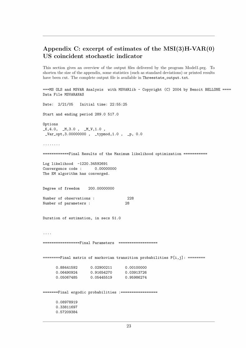
Appendix C: excerpt of estimates of the MSI(3)H-VAR(0)US coincident stochastic indicator

This section gives an overview of the output files delivered by the program Model1.prg. Toshorten the size of the appendix, some statistics (such as standard deviations) or printed resultshave been cut. The complete output file is available in Threestate_output.txt.

===MS OLS and MSVAR Analysis with MSVARlib - Copyright (C) 2004 by Benoit BELLONE ====Data File MSVARANAS

Date: 2/21/05 Initial time: 22:55:25

Start and ending period 289.0 517.0

Options_K,4.0, _M,3.0 , _M_V,1.0 ,_Var_opt,3.00000000 , _typmod,1.0 , _p, 0.0

........

============Final Results of the Maximum likelihood optimization ===========

Log likelihood -1220.34592691Convergence code : 0.00000000The EM algorithm has converged.

Degree of freedom 200.00000000

Number of observations : 228Number of parameters : 28

Duration of estimation, in secs 51.0

....

=================Final Parameters ==================

========Final matrix of markovian transition probabilities P[i,j]: ========

0.88441592 0.02900211 0.001000000.06490924 0.91654270 0.039137260.05067485 0.05445519 0.95986274

=======Final ergodic probabilities :=================

0.089789190.338116970.57209384

23

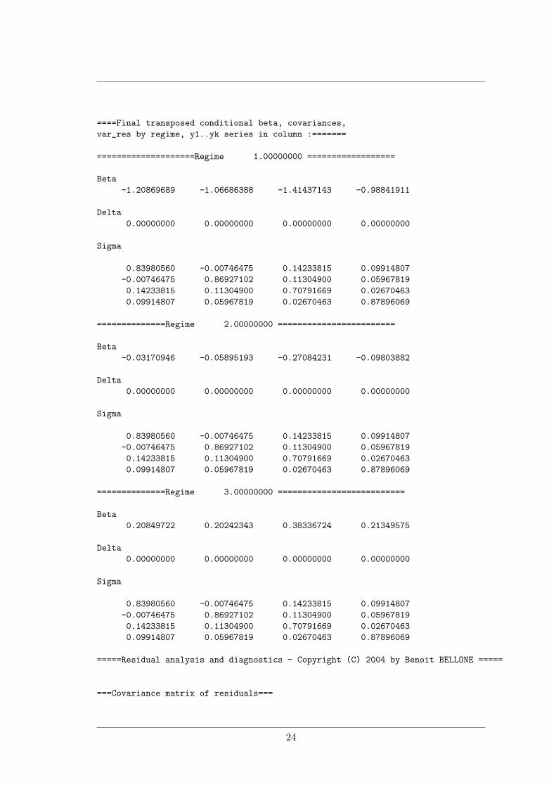
====Final transposed conditional beta, covariances,var_res by regime, y1..yk series in column :=======

====================Regime 1.00000000 ==================

Beta-1.20869689 -1.06686388 -1.41437143 -0.98841911

Delta0.00000000 0.00000000 0.00000000 0.00000000

Sigma

0.83980560 -0.00746475 0.14233815 0.09914807-0.00746475 0.86927102 0.11304900 0.059678190.14233815 0.11304900 0.70791669 0.026704630.09914807 0.05967819 0.02670463 0.87896069

==============Regime 2.00000000 ========================

Beta-0.03170946 -0.05895193 -0.27084231 -0.09803882

Delta0.00000000 0.00000000 0.00000000 0.00000000

Sigma

0.83980560 -0.00746475 0.14233815 0.09914807-0.00746475 0.86927102 0.11304900 0.059678190.14233815 0.11304900 0.70791669 0.026704630.09914807 0.05967819 0.02670463 0.87896069

==============Regime 3.00000000 ==========================

Beta0.20849722 0.20242343 0.38336724 0.21349575

Delta0.00000000 0.00000000 0.00000000 0.00000000

Sigma

0.83980560 -0.00746475 0.14233815 0.09914807-0.00746475 0.86927102 0.11304900 0.059678190.14233815 0.11304900 0.70791669 0.026704630.09914807 0.05967819 0.02670463 0.87896069

=====Residual analysis and diagnostics - Copyright (C) 2004 by Benoit BELLONE =====

===Covariance matrix of residuals===

24

0.83171267 -0.01624330 0.10779953 0.08437932-0.01624330 0.86119396 0.08333086 0.047309170.10779953 0.08333086 0.61427796 -0.009529720.08437932 0.04730917 -0.00952972 0.86345343

=== Information Criteria based upon Residual Covariance Matrix Analysis ===----------------------------------------------------------------------------

BIC AICa AICc SIC FPE AIC HQ----------------------------------------------------------------------------

-0.639 -0.809 0.120 0.629 0.430 -0.880 -0.782

====== Multivariate analysis of residuals - Jarque Berra ===================

Jarque and Bera Test, Under Ho : ’Residuals are normal’JB stat: 13.112Pvalue : 0.108The Normality hypothesis cannot be rejected

25

Figure 8: MSI(3)H-VAR(0) - Filtered probabilities

26

Figure 9: MSI(3)H-VAR(0)- Smoothed probabilities

27