Methodology for stress

evaluation in pipe branch

connections

Alexander Eriksson

Supervisor at LiU: Bo Torstenfelt

Examiner at LiU: Daniel Leidermark

Supervisor at Ingenjörsfirman Rörkraft AB: Anders Wetterberg

ISRN: LIU-IEI-TEK-A--15/02115—SE

Division of Solid Mechanics

Department of Management and Engineering

Linköping University

ii

iii

Preface

This work is a thesis for the Master of Science degree in Mechanical Engineering at Linköping

University. It was carried out within the master’s program in Mechanical Engineering during spring of

2014.

During the project a method for evaluating stresses in unreinforced pipe branch connections has

been created. The method can be used to make a fast evaluation of any pipe branch geometry. The

method is made in coordination with the standards EN 13480-3 and EN 13445-3 and supplemented

with ASME VIII div 2 part 5 and articles concerning the subject. The initiator of this projected was

Rörkraft AB and my advisor Anders Wetterberg was the major contributor.

I would like to express my thanks to my advisor at Rörkraft AB, Anders Wetterberg, for his support,

patience and guidance during this thesis. I also would like to give my thanks to my loving and

supporting wife, Elena.

Finally I want to thank my supervisor at the Division of Solid Mechanics at Linköping University, Bo

Torstenfelt, for his patience and support.

Lund, November 2014

Alexander Eriksson

iv

v

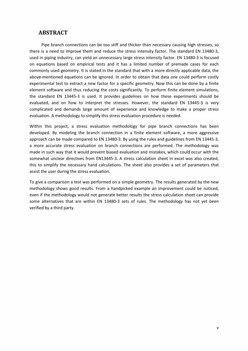
ABSTRACT

Pipe branch connections can be too stiff and thicker than necessary causing high stresses, so

there is a need to improve them and reduce the stress intensity factor. The standard EN 13480-3,

used in piping industry, can yield an unnecessary large stress intensity factor. EN 13480-3 is focused

on equations based on empirical tests and it has a limited number of premade cases for each

commonly used geometry. It is stated in the standard that with a more directly applicable data, the

above-mentioned equations can be ignored. In order to obtain that data one could perform costly

experimental test to extract a new factor for a specific geometry. Now this can be done by a finite

element software and thus reducing the costs significantly. To perform finite element simulations,

the standard EN 13445-3 is used. It provides guidelines on how these experiments should be

evaluated, and on how to interpret the stresses. However, the standard EN 13445-3 is very

complicated and demands large amount of experience and knowledge to make a proper stress

evaluation. A methodology to simplify this stress evaluation procedure is needed.

Within this project, a stress evaluation methodology for pipe branch connections has been

developed. By modeling the branch connection in a finite element software, a more aggressive

approach can be made compared to EN 13480-3. By using the rules and guidelines from EN 13445-3,

a more accurate stress evaluation on branch connections are performed. The methodology was

made in such way that it would prevent biased evaluation and mistakes, which could occur with the

somewhat unclear directives from EN13445-3. A stress calculation sheet in excel was also created,

this to simplify the necessary hand calculations. The sheet also provides a set of parameters that

assist the user during the stress evaluation.

To give a comparison a test was performed on a simple geometry. The results generated by the new

methodology shows good results. From a handpicked example an improvement could be noticed,

even if the methodology would not generate better results the stress calculation sheet can provide

some alternatives that are within EN 13480-3 sets of rules. The methodology has not yet been

verified by a third party.

vi

vii

NOMENCLATURE

ABBREVIATIONS

FEA Finite Element Analysis

FEM Finite Element Model

SIF Stress Intensity Factor

VM Von Mises

Pm Membrane stress

Pb Bending stress

Q Secondary stress

F Peak stress

𝜎1,2,3 Principal stress

SCL Stress classification line

PVD Pressure vessel design

viii

Contents Preface ..................................................................................................................................................... iii

ABSTRACT ................................................................................................................................................. v

1 Introduction ..................................................................................................................................... 1

1.1 Background .............................................................................................................................. 1

1.2 Objective.................................................................................................................................. 2

1.3 Approach ................................................................................................................................. 2

1.4 Limitations ............................................................................................................................... 2

1.5 Other considerations ............................................................................................................... 2

2 Theory .............................................................................................................................................. 3

2.1 Standard EN 13480-3 ............................................................................................................... 3

2.2 Stress Intensity Factor ............................................................................................................. 5

2.3 Standard EN 13445-3 ............................................................................................................... 9

3 CAEPIPE ......................................................................................................................................... 15

3.1 Calculation ............................................................................................................................. 15

3.2 Model .................................................................................................................................... 16

4 Autodesk Simulation Mechanical .................................................................................................. 18

4.1 Shell model ............................................................................................................................ 19

4.2 Solid model ............................................................................................................................ 21

5 Stress evaluation method .............................................................................................................. 22

6 Results ........................................................................................................................................... 23

6.1 Testing the method ............................................................................................................... 24

7 Discussion ...................................................................................................................................... 26

8 Conclusion ..................................................................................................................................... 28

9 References ..................................................................................................................................... 29

10 Appendix .................................................................................................................................... 30

10.1 Boundary condition sensitivity study .................................................................................... 30

10.2 Excel sheet ............................................................................................................................. 31

10.2.1 Stress calculation sheet ................................................................................................. 32

10.3 Linearization .......................................................................................................................... 35

ix

List of Figures

Figure 1, Unreinforced fabricated branch pipe with declared dimensions (EN 13480-3, 2012) ............ 3

Figure 2, The three different setups with boundary conditions shown loaded at point F, which Markl

tested ....................................................................................................................................................... 5

Figure 3, S-N curve with an example of extracting SIF [8] ...................................................................... 6

Figure 4, The loads on a branch connection ........................................................................................... 7

Figure 5, Stress categorization from EN 13445-3 [4] ............................................................................ 10

Figure 6, Opening in a shell, point 1 for run pipe, 2 for branch pipe, 3 for local region and 4 defines

the limit for local region [3] ................................................................................................................... 11

Figure 7, Cross section of run/branch pipe junction [9] ........................................................................ 12

Figure 8, Supporting line segment and local axis in which the elementary stresses are expressed,

where 1 is pointing at two different supporting line segments [3] ...................................................... 13

Figure 9, Decomposition of the longitudinal stress on a shell due to external bending moment M [3]

............................................................................................................................................................... 14

Figure 10, Branch connection modeled in CAEPIPE with 4 nodes and 3 pipe elements ....................... 15

Figure 11, CAEPIPE displaying reaction forces for each node on a branch connection. ....................... 17

Figure 12, Two branch connection, solid elements to the left and shell elements to the right ........... 18

Figure 13, Mesh divisions of a PVD model, show four in mesh division ............................................... 18

Figure 14, Junction of a tee with two nodes chosen as probes for stress results. ................................ 20

Figure 15, A simplified sketch to show where the evaluation point are located on the branch pipe. . 23

x

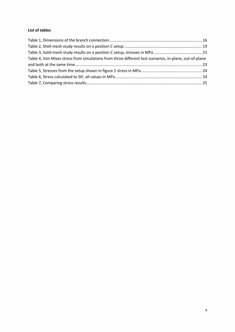
List of tables

Table 1, Dimensions of the branch connection ..................................................................................... 16

Table 2, Shell mesh study results on a position C setup ....................................................................... 19

Table 3, Solid mesh study results on a position C setup, stresses in MPa ............................................ 21

Table 4, Von Mises stress from simulations from three different test scenarios, in-plane, out-of-plane

and both at the same time .................................................................................................................... 23

Table 5, Stresses from the setup shown in figure 2 stress in MPa ........................................................ 24

Table 6, Stress calculated to SIF, all values in MPa ............................................................................... 24

Table 7, Comparing stress results.......................................................................................................... 25

1

1 Introduction This work is performed at Ingenjörsfirman Rörkraft AB in Lund. Rörkraft is a pipe construction

company which delivers complete piping solutions. Their market consists of everything from nuclear

power plants to small municipal heating plants and processing plants which range from pulp to food

processing. Their clients include Tetra Pak, Karlshamn Kraft AB and Södra Cell Mörrum. Rörkraft

delivers piping solutions that do not depend on any specific type of weld, which enables the

customer to have a greater opportunity to choose a welder who can choose a type of weld that they

are certified to perform. The piping industries in Europe are mainly using the standard EN 13480-3 [1]

to calculate the stresses in different tubular joints and this calculation procedure is based on

analytical and experimental data. The mentioned standards cover any type of load case and static

and dynamic loading. First of all the classification is made depending on the purpose of usage and

conditions it has to operate in (i.e. metallic industrial piping, non-heat transferring pressure vessels)

and the appropriate standard is chosen. For metallic piping in particular, Rörkraft is using the

standard EN 13480-3. However, it is commonly known in the piping industry community that EN

13480-3 is conservative in terms of how the Stress Intensity Factor (SIF) is calculated in branch

connections. This makes them thicker than they need to be, thus making them stiffer and heavier

which is not desirable. Reducing the SIF will not only help the costumers save money but also keep a

sustainable development of emerging economies and have a lesser impact on the environment. This

work is motivated by the statement in EN 13480-3: “In the absence of more directly applicable data,

the flexibility factors and stress intensification factors shown in Annex H, shall be used in flexibility

calculation.” Therefore a study will be performed to find the applicable data.

1.1 Background There are two methods which are used by Rörkraft today, one is using CAEPIPE [2] in

combination with the standard EN 13480-3 to perform the analysis of the piping system. The

customer declares the purpose and location of the piping system and its dimensions, if existing.

Rörkraft models the piping system in CAEPIPE, adding all the prescribed loads such as wind, pressure,

temperature etc. from the costumer’s specifications and geometrical obstacles. In combination with

CAEPIPE and the standard, relevant for the specific system, the piping system can be validated and

approved for service. However it is important to remember that CAEPIPE considers all loads as one

type of load, which is conservative approach. This procedure analyzes the whole model and if any

stress is above yield limit specified in CAEPIPE then different resizing and scaling actions are

performed until the stresses are in an acceptable range. Branch pipes can be a source causing high

stresses due to structural discontinuities. In the general case fatigue assessment is excluded since the

number load cycles are considered to be low.

The other method is design by analysis which is stated in EN 13445-3 [3] and use of Finite Element

Analysis (FEA) to validate a certain design. However the FE-model needs to be made for each case

and meshed accordingly. This can be very time consuming, since many systems are very large and

this often needs to be validated by a third party . If a small changes to the stress the whole procedure

need to be reevaluated again.

2

1.2 Objective The objective of this work is to develop a method that calculates a less conservative SIF and

also develop an alternative way of calculating SIF for an “in-plane load case”.

1.3 Approach The approach in this work will be investigating a pipe branch. The pipe branch will have a set

of predefined parameters and a set of load cases which will be considered. The standards that are

involved in calculations of a pipe branch will be examined and articles which can provide additional

information will be reviewed. Using the knowledge from the articles and following the criteria from

the standards, a FEA will be performed on a test piece. Focus will be on static stresses only due to

mechanical loads, no thermal loads will be considered. Finite Element (FE) simulation will be

performed on a pipe branch which will be investigated for different load cases. This work will use the

same software as Rörkraft which is Autodesk Simulation Mechanical [4] and CAEPIPE. Currently the

SIF is calculated from an empirical equation, which comes from experimental tests, derived by A.R.C

Markl [5] which is known to be conservative. In FEA the SIF might be lower and thus a more

profitable approach can be found when it comes to designing piping branches. Both solid and shell

models will be investigated and two options will be presented and compared. This work will present

three different methods; stress evaluation by using only CAEPIPE, stress evaluation by using CAEPIPE

combined with the alternative way of calculating the “corrected SIF” and stress evaluation using the

method developed in this work.

Fatigue assessment will not be taken into consideration since the typical loading scenario is

considered to be low cycle, N<7000 where N is the number of cycles. The stresses from the simulated

model will be evaluated according to EN-13445-3. An excel sheet, see Appendix 10.2, which simplifies

a calculation of a new SIF will be designed. The excel sheet will also show the old SIF in such a way

that the user can compare different SIF results, without entering CAEPIPE. The excel sheet will also

calculate less conservative SIF from EN 13480-3. When the new SIF is compared with the old in the

excel sheet, it can be inserted into CAEPIPE.

1.4 Limitations No weld

No reinforced branch

No torque

No pressure

No fatigue

Only 90° degree branch

No thermal stress

1.5 Other considerations No ethical or gender issues are raised in this thesis.

3

2 Theory The theoretical part of this work is divided in to three parts: The Stress Intensity Factor,

Standard EN 13480-3 and Standard EN 13445-3. This split was necessary because of the differences

in the approach of the two standards. EN 13480-3 uses predefined equations to determine the

stresses. Those equations are based on experimental tests and analytical solutions. On the other

hand, the method described in EN 13445-3 is based on stress categories which are calculated for

each single case that is investigated and those stresses are not determined by equations but are

rather derived by experimental tests or FEA.

2.1 Standard EN 13480-3 EN 13480-3 is the European standard for metallic industrial piping that deals with design and

calculations. The standard describes how the stresses should be calculated by hand. The focus will be

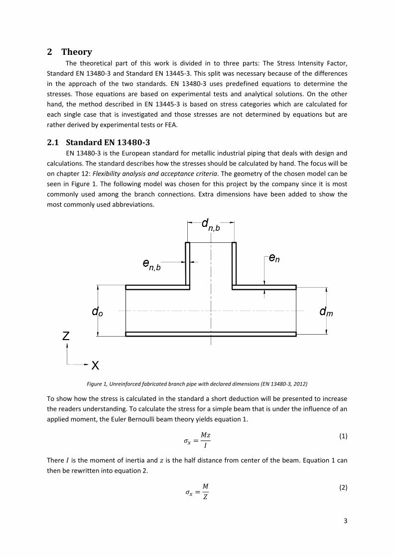
on chapter 12: Flexibility analysis and acceptance criteria. The geometry of the chosen model can be

seen in Figure 1. The following model was chosen for this project by the company since it is most

commonly used among the branch connections. Extra dimensions have been added to show the

most commonly used abbreviations.

Figure 1, Unreinforced fabricated branch pipe with declared dimensions (EN 13480-3, 2012)

To show how the stress is calculated in the standard a short deduction will be presented to increase

the readers understanding. To calculate the stress for a simple beam that is under the influence of an

applied moment, the Euler Bernoulli beam theory yields equation 1.

𝜎𝑥 =

𝑀𝑧

𝐼

(1)

There 𝐼 is the moment of inertia and 𝑧 is the half distance from center of the beam. Equation 1 can

then be rewritten into equation 2.

𝜎𝑥 =

𝑀

𝑍

(2)

4

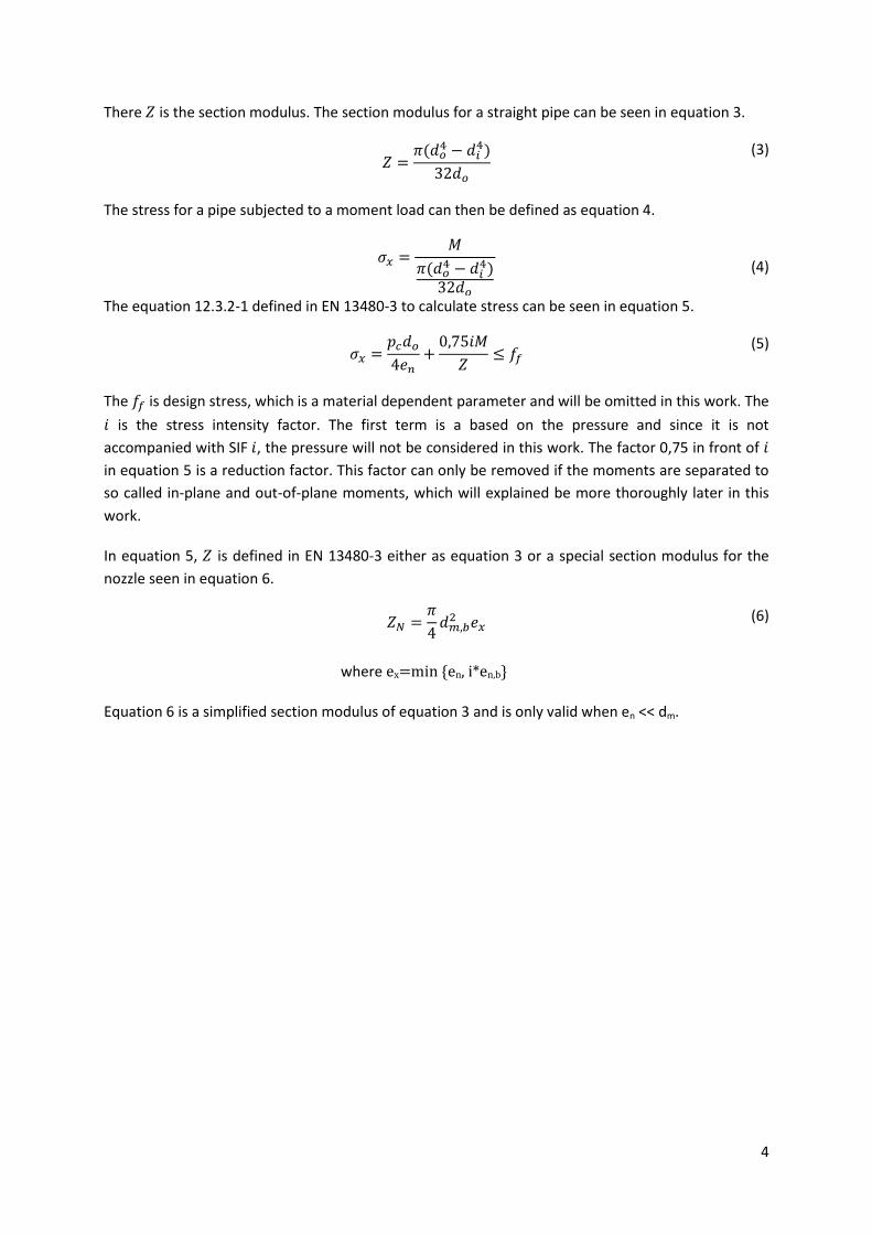
There 𝑍 is the section modulus. The section modulus for a straight pipe can be seen in equation 3.

𝑍 =

𝜋(𝑑𝑜4 − 𝑑𝑖

4)

32𝑑𝑜

(3)

The stress for a pipe subjected to a moment load can then be defined as equation 4.

𝜎𝑥 =

𝑀

𝜋(𝑑𝑜4 − 𝑑𝑖

4)32𝑑𝑜

(4)

The equation 12.3.2-1 defined in EN 13480-3 to calculate stress can be seen in equation 5.

𝜎𝑥 =

𝑝𝑐𝑑𝑜

4𝑒𝑛+

0,75𝑖𝑀

𝑍≤ 𝑓𝑓

(5)

The 𝑓𝑓 is design stress, which is a material dependent parameter and will be omitted in this work. The

𝑖 is the stress intensity factor. The first term is a based on the pressure and since it is not

accompanied with SIF 𝑖, the pressure will not be considered in this work. The factor 0,75 in front of 𝑖

in equation 5 is a reduction factor. This factor can only be removed if the moments are separated to

so called in-plane and out-of-plane moments, which will explained be more thoroughly later in this

work.

In equation 5, 𝑍 is defined in EN 13480-3 either as equation 3 or a special section modulus for the

nozzle seen in equation 6.

𝑍𝑁 =𝜋

4𝑑𝑚,𝑏

2 𝑒𝑥 (6)

where ex=min {en, i*en,b}

Equation 6 is a simplified section modulus of equation 3 and is only valid when en << dm.

5

2.2 Stress Intensity Factor In the 1950’s there was a need to improve the safety of piping against failure without the use

of excessive reinforcement that made pipe branches unnecessary large. With this in mind, A.R.C

Markl performed a series of tests on a pipe branch. This was needed to determine how to calculate

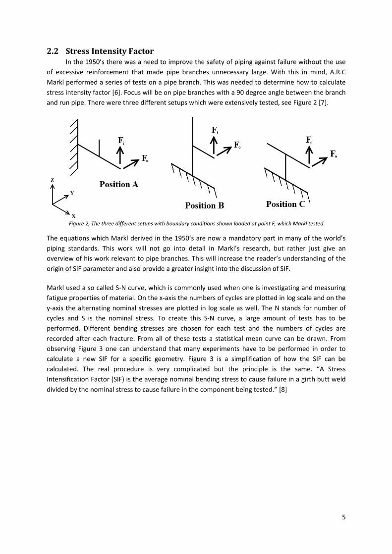
stress intensity factor [6]. Focus will be on pipe branches with a 90 degree angle between the branch

and run pipe. There were three different setups which were extensively tested, see Figure 2 [7].

Figure 2, The three different setups with boundary conditions shown loaded at point F, which Markl tested

The equations which Markl derived in the 1950’s are now a mandatory part in many of the world’s

piping standards. This work will not go into detail in Markl’s research, but rather just give an

overview of his work relevant to pipe branches. This will increase the reader’s understanding of the

origin of SIF parameter and also provide a greater insight into the discussion of SIF.

Markl used a so called S-N curve, which is commonly used when one is investigating and measuring

fatigue properties of material. On the x-axis the numbers of cycles are plotted in log scale and on the

y-axis the alternating nominal stresses are plotted in log scale as well. The N stands for number of

cycles and S is the nominal stress. To create this S-N curve, a large amount of tests has to be

performed. Different bending stresses are chosen for each test and the numbers of cycles are

recorded after each fracture. From all of these tests a statistical mean curve can be drawn. From

observing Figure 3 one can understand that many experiments have to be performed in order to

calculate a new SIF for a specific geometry. Figure 3 is a simplification of how the SIF can be

calculated. The real procedure is very complicated but the principle is the same. “A Stress

Intensification Factor (SIF) is the average nominal bending stress to cause failure in a girth butt weld

divided by the nominal stress to cause failure in the component being tested.” [8]

6

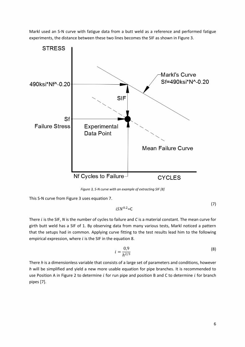
Markl used an S-N curve with fatigue data from a butt weld as a reference and performed fatigue

experiments, the distance between these two lines becomes the SIF as shown in Figure 3.

Figure 3, S-N curve with an example of extracting SIF [8]

This S-N curve from Figure 3 uses equation 7.

𝑖𝑆𝑁0.2=C (7)

There 𝑖 is the SIF, N is the number of cycles to failure and C is a material constant. The mean curve for

girth butt weld has a SIF of 1. By observing data from many various tests, Markl noticed a pattern

that the setups had in common. Applying curve fitting to the test results lead him to the following

empirical expression, where 𝑖 is the SIF in the equation 8.

𝑖 =

0,9

ℎ2/3

(8)

There h is a dimensionless variable that consists of a large set of parameters and conditions, however

h will be simplified and yield a new more usable equation for pipe branches. It is recommended to

use Position A in Figure 2 to determine 𝑖 for run pipe and position B and C to determine 𝑖 for branch

pipes [7].

7

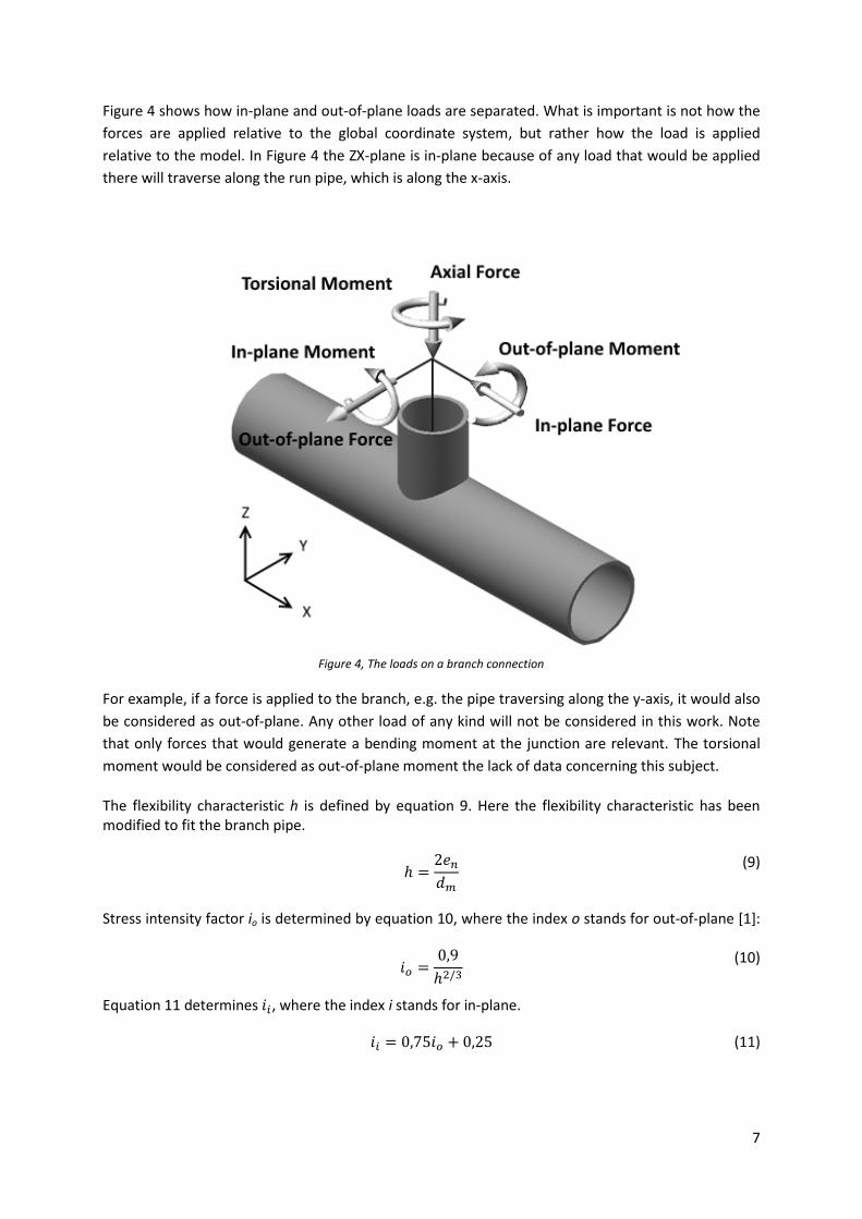
Figure 4 shows how in-plane and out-of-plane loads are separated. What is important is not how the

forces are applied relative to the global coordinate system, but rather how the load is applied

relative to the model. In Figure 4 the ZX-plane is in-plane because of any load that would be applied

there will traverse along the run pipe, which is along the x-axis.

Figure 4, The loads on a branch connection

For example, if a force is applied to the branch, e.g. the pipe traversing along the y-axis, it would also

be considered as out-of-plane. Any other load of any kind will not be considered in this work. Note

that only forces that would generate a bending moment at the junction are relevant. The torsional

moment would be considered as out-of-plane moment the lack of data concerning this subject.

The flexibility characteristic h is defined by equation 9. Here the flexibility characteristic has been modified to fit the branch pipe.

ℎ =

2𝑒𝑛

𝑑𝑚

(9)

Stress intensity factor io is determined by equation 10, where the index o stands for out-of-plane [1]:

𝑖𝑜 =0,9

ℎ2/3

(10)

Equation 11 determines 𝑖𝑖, where the index i stands for in-plane.

𝑖𝑖 = 0,75𝑖𝑜 + 0,25 (11)

8

Here we can also see how the standard separates in and out-of-plane with two equations. As it was

mentioned in the Background, CAEPIPE considers all loads as out-of-plane which is based on

equation 10.

From equation 9 and 10 we receive equation 12 and similarly we receive 13 from 11 and 12.

𝑖𝑜 =

0,9

(2𝑒𝑛𝑑𝑚

)2/3

(12)

𝑖𝑖 = 0,75

0,9

(2𝑒𝑛𝑑𝑚

)2/3

+ 0,25

(13)

Equation 12 and 13 will be used in the excel sheet to lower the SIF, which will be referred to as the

corrected SIF as an alternative stress evaluation method, when the SIF from FEA cannot yield better

results. This will be explained more in Appendix 10.2.

9

2.3 Standard EN 13445-3 EN 13445-3 is the European standard for non-heat accepting pressure vessels which is called

“Unfired pressure vessels”. In this work the chapter Annex C: Design by analysis – Method based on

stress categories will be considered. It provides “rules concerning design by analysis using stress

classification” [3]. Those rules are applicable to branch connections, if a pressure vessel is considered

to be of the same size as the run pipe and with an attached nozzle on the side with dimensions as the

branch pipe. Standard EN 13445-3 governs how the stresses should be calculated and categorized in

pressure vessels.

According to EN 13445-3 the six elementary stresses (𝜎𝑖𝑗) should be determined by experimental

tests or by calculations with the following assumptions:

Material behavior is linear isotropic elastic in accordance with Hooke’s law

Displacements and strains are small according to first order theory

This work will make use of calculations to determine the stresses mainly because experimental tests

are costly and difficult. The stresses will be calculated by using the FE-software Autodesk Simulation

Mechanical [4]. The standard suggests representing the stresses either by Tresca or Von Mises. Von

Mises is known to have a smoother yield surface compared to Tresca. Von Mises yield criterion can

be seen in equation 14.

𝜎𝑉𝑀 = √𝜎1

2 + 𝜎22+𝜎3

2 − 𝜎1𝜎2 − 𝜎2𝜎3 − 𝜎3𝜎1 (14)

There 𝜎1,2,3 are the principal stresses. The categorization, that EN 13445-3 in (Annex C) suggests the

user to perform, is not necessary in this case, because this work is focused on evaluating the stress

response from the load, and not on preventing pipe branches against yielding which is the main focus

of EN 13445-3. Although Annex C categorization procedure will not be used, it does give valuable

information of where to perform these evaluations and how to extract the stresses.

The Von Mises stress and total stress are the same in this work, because there is no internal

pressure.

10

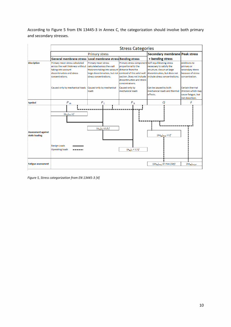
According to Figure 5 from EN 13445-3 in Annex C, the categorization should involve both primary

and secondary stresses.

Figure 5, Stress categorization from EN 13445-3 [4]

11

According to Porter et al. [9] these categories depend on where the evaluation takes place and what

the level of stresses is. Note that American Society of Mechanical Engineers (ASME), which is the

American standard, is being studied in Porter et al [9] and EN is used in this work. However, both

standards are using the same categorization, meaning that the stress relative the global stress limit f,

decides where different stresses reside, as seen in Figure 5.

The important part in this work is to know where to evaluate, more specifically how far away from

the junction between nozzle and run pipe. Peak stresses are associated with fatigue [3] which can be

seen in Figure 5 and those stresses are omitted in this work. The question will be where these

stresses are situated. According to Porter et al. [9], they are confined within the vicinity of the

junction. In this work the focus will only be on the total stress and peak stress will be excluded.

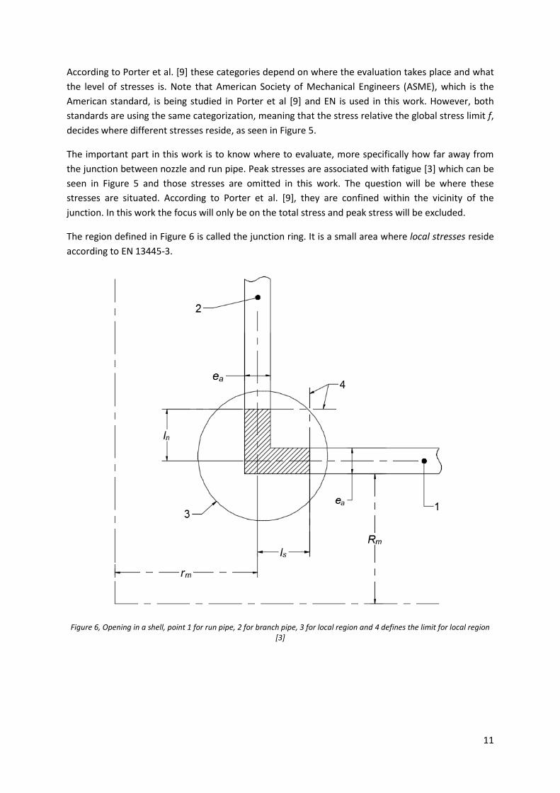
The region defined in Figure 6 is called the junction ring. It is a small area where local stresses reside

according to EN 13445-3.

Figure 6, Opening in a shell, point 1 for run pipe, 2 for branch pipe, 3 for local region and 4 defines the limit for local region [3]

12

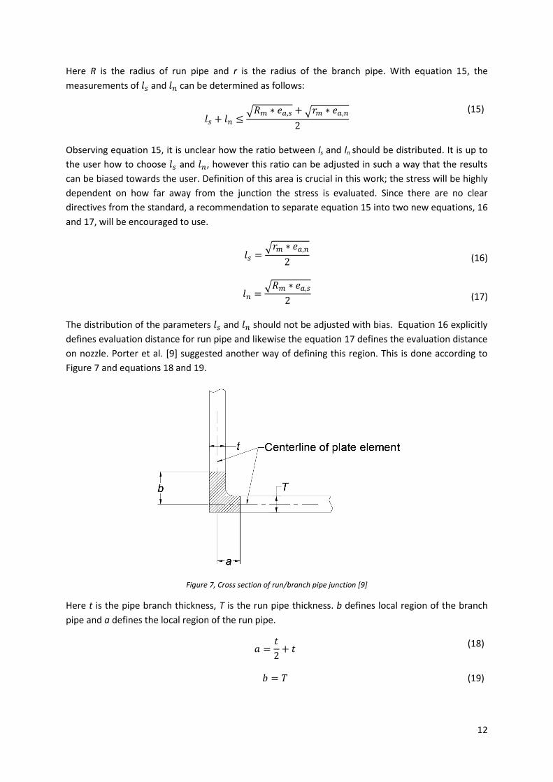
Here R is the radius of run pipe and r is the radius of the branch pipe. With equation 15, the

measurements of 𝑙𝑠 and 𝑙𝑛 can be determined as follows:

𝑙𝑠 + 𝑙𝑛 ≤

√𝑅𝑚 ∗ 𝑒𝑎,𝑠 + √𝑟𝑚 ∗ 𝑒𝑎,𝑛

2

(15)

Observing equation 15, it is unclear how the ratio between ls and ln should be distributed. It is up to

the user how to choose 𝑙𝑠 and 𝑙𝑛, however this ratio can be adjusted in such a way that the results

can be biased towards the user. Definition of this area is crucial in this work; the stress will be highly

dependent on how far away from the junction the stress is evaluated. Since there are no clear

directives from the standard, a recommendation to separate equation 15 into two new equations, 16

and 17, will be encouraged to use.

𝑙𝑠 =

√𝑟𝑚 ∗ 𝑒𝑎,𝑛

2

(16)

𝑙𝑛 =

√𝑅𝑚 ∗ 𝑒𝑎,𝑠

2

(17)

The distribution of the parameters 𝑙𝑠 and 𝑙𝑛 should not be adjusted with bias. Equation 16 explicitly

defines evaluation distance for run pipe and likewise the equation 17 defines the evaluation distance

on nozzle. Porter et al. [9] suggested another way of defining this region. This is done according to

Figure 7 and equations 18 and 19.

Figure 7, Cross section of run/branch pipe junction [9]

Here t is the pipe branch thickness, T is the run pipe thickness. b defines local region of the branch

pipe and a defines the local region of the run pipe.

𝑎 =

𝑡

2+ 𝑡

(18)

𝑏 = 𝑇 (19)

13

There are some major differences between those two methods; EN 13445-3 is based on the diameter

of the connecting pipes and has no defined distribution between 𝑙𝑠 and 𝑙𝑛 and will generally also be

less conservative, whereas the second method suggested by Porter el al. [9] depends only on the

thickness of the nozzle and the distribution between 𝑎 and 𝑏 is predefined.

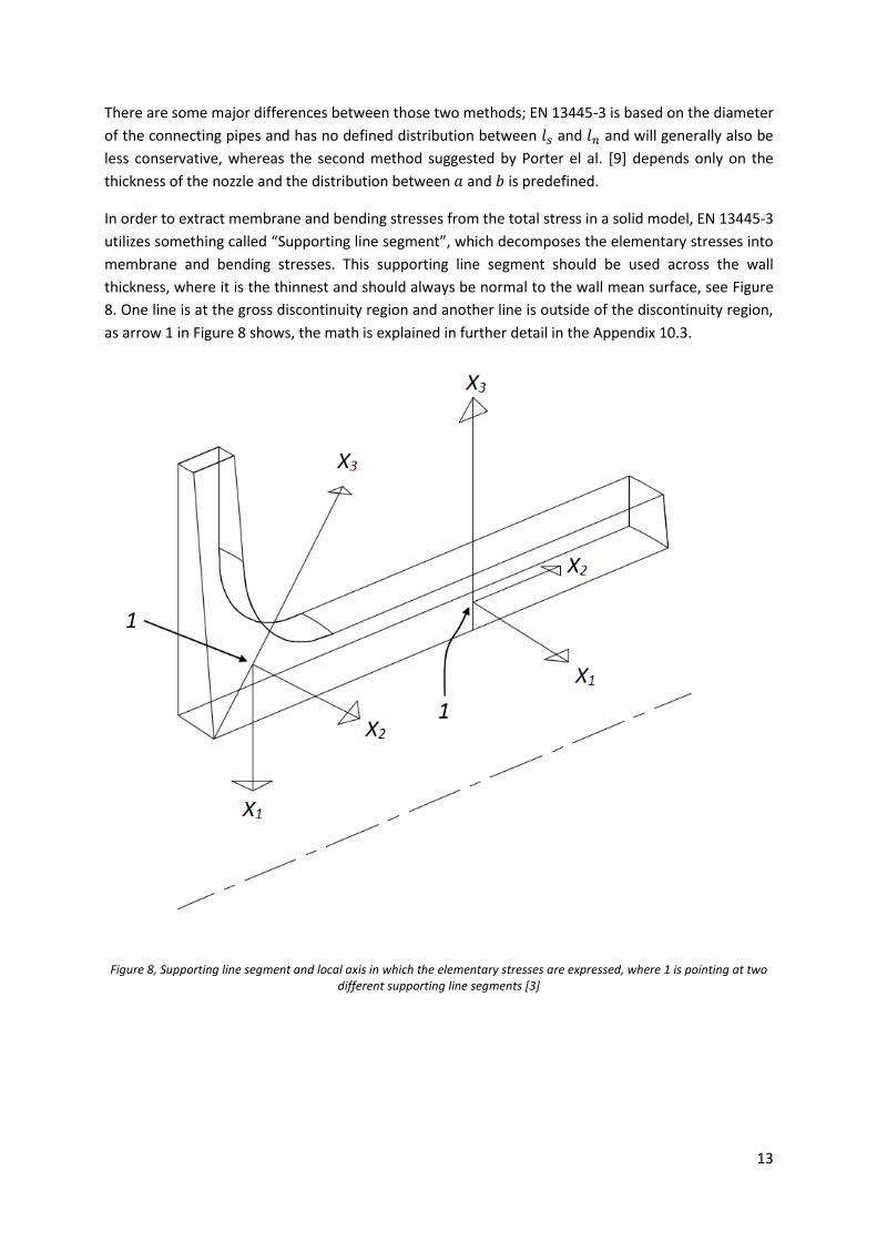
In order to extract membrane and bending stresses from the total stress in a solid model, EN 13445-3

utilizes something called “Supporting line segment”, which decomposes the elementary stresses into

membrane and bending stresses. This supporting line segment should be used across the wall

thickness, where it is the thinnest and should always be normal to the wall mean surface, see Figure

8. One line is at the gross discontinuity region and another line is outside of the discontinuity region,

as arrow 1 in Figure 8 shows, the math is explained in further detail in the Appendix 10.3.

Figure 8, Supporting line segment and local axis in which the elementary stresses are expressed, where 1 is pointing at two different supporting line segments [3]

14

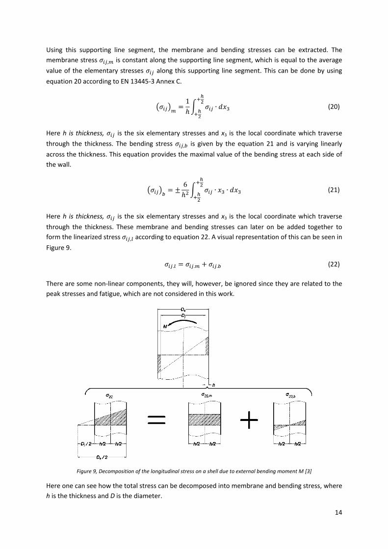
Using this supporting line segment, the membrane and bending stresses can be extracted. The

membrane stress 𝜎𝑖𝑗,𝑚 is constant along the supporting line segment, which is equal to the average

value of the elementary stresses 𝜎𝑖𝑗 along this supporting line segment. This can be done by using

equation 20 according to EN 13445-3 Annex C.

(𝜎𝑖𝑗)

𝑚=

1

ℎ∫ 𝜎𝑖𝑗

+ℎ2

+ℎ2

∙ 𝑑𝑥3

(20)

Here h is thickness, 𝜎𝑖𝑗 is the six elementary stresses and x3 is the local coordinate which traverse

through the thickness. The bending stress 𝜎𝑖𝑗,𝑏 is given by the equation 21 and is varying linearly

across the thickness. This equation provides the maximal value of the bending stress at each side of

the wall.

(𝜎𝑖𝑗)

𝑏= ±

6

ℎ2∫ 𝜎𝑖𝑗

+ℎ2

+ℎ2

∙ 𝑥3 ∙ 𝑑𝑥3

(21)

Here h is thickness, 𝜎𝑖𝑗 is the six elementary stresses and x3 is the local coordinate which traverse

through the thickness. These membrane and bending stresses can later on be added together to

form the linearized stress 𝜎𝑖𝑗,𝑙 according to equation 22. A visual representation of this can be seen in

Figure 9.

𝜎𝑖𝑗.𝑙 = 𝜎𝑖𝑗.𝑚 + 𝜎𝑖𝑗.𝑏 (22)

There are some non-linear components, they will, however, be ignored since they are related to the

peak stresses and fatigue, which are not considered in this work.

Figure 9, Decomposition of the longitudinal stress on a shell due to external bending moment M [3]

Here one can see how the total stress can be decomposed into membrane and bending stress, where

h is the thickness and D is the diameter.

15

3 CAEPIPE CAEPIPE is exclusively made to model and perform standard based calculations on arbitrary

large piping systems. The standard which CAEPIPE should employ can be chosen in the settings. To

mention a few which CAEPIPE can follow: EN-13480-3, ASME B31.1, ASME B31.2 and so on. This

program aids the engineer in terms of calculations when it comes to the predefined equations that

are declared in the standards and automatically calculates the reaction forces and moments that

occur throughout the piping system.

3.1 Calculation CAEPIPE is using the standards as reference to perform its calculations. For the purpose of this

work CAEPIPE will be set to the standard EN 13480-3. There are different types of elements to

choose from in CAEPIPE, in this work pipe elements will be used. According to equation 23, the pipe

elements formulation is based only on a pressure and moment and each element is connected in one

node on each side.

𝜎 =

𝑝𝑐𝑑𝑜

4𝑒𝑛+

𝑀

𝑍

(23)

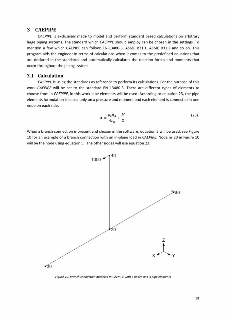
When a branch connection is present and chosen in the software, equation 5 will be used, see Figure

10 for an example of a branch connection with an in-plane load in CAEPIPE. Node nr 20 in Figure 10

will be the node using equation 5. The other nodes will use equation 23.

Figure 10, Branch connection modeled in CAEPIPE with 4 nodes and 3 pipe elements

16

Node nr 20 can be changed in the input window to have an automatic SIF value and follow equation

9 and 10 or the user can chose to input a SIF value manually. When the non-automatic number is

used, CAEPIPE will use equation 5. However, it will not use equation 9 and 10 because the SIF is now

inserted manually. In addition it will also use equation 3 which is the analytical section modulus

equation and not the special one for nozzle as equation 6 describes.

The user SIF which will be used in CAEPIPE can be calculated by equation 24.

𝑆𝐼𝐹 =𝜎𝐹𝐸𝑀

𝜎𝑛𝑜𝑚 (24)

The value 𝜎𝑛𝑜𝑚 will be calculated by hand from equation 25. M will be the resultant moment and Z

will be the section modulus according to equation 3.

𝜎𝑛𝑜𝑚 =

𝑀

𝑍

(25)

The stress 𝜎𝐹𝐸𝑀 will be extracted from the FEA which will be explained more thoroughly later on in

this work.

As it is known, loads can be either out-of-plane or in-plane. CAEPIPE considers all the loads as out-of-

plane, however, the standard EN 13480-3 has one extra equation for in-plane load. That means that

by using equations from the standard it is possible to calculate the in-plane SIF and adapt it to

CAEPIPE. This issue will also be addressed in the method development. By considering both out-of-

plane and in-plane loads, a new SIF will be calculated. It will be valid in CAEPIPE in such a way that if

a change in forces occurs, the user will not have to perform another simulation of the FEM and

evaluate the stresses.

3.2 Model The model used in this thesis will be an unreinforced pipe branch connection from Figure 1

with the dimensions which can be seen in Table 1. These dimensions were suggested by Rörkraft.

Since the purpose of this work is to develop a method independent of dimensions, it is of little

importance what dimensions are being used. The force to be applied to the model should be

relatively low, due to the fact that only elastic region is being studied. The force that generates the

stress should always be lower than yield stress of the material to avoid any plasticity. The SIF is

calculated from equation 24, thus it is only the stress response needed to receive desired results.

Table 1, Dimensions of the branch connection

Branch connection Run Pipe Branch Pipe

Diameter (do) [mm] 219.1 139.7

Thickness (en, eb)[mm] 6.3 4

Density [Kg/m^3] 7850 7850

Young’s modulus

[GPa]

212 212

Poison’s Ratio 0.3 0.3

Length [mm] 1000 (total) 500

17

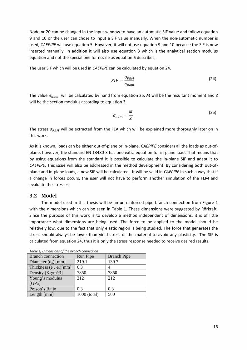
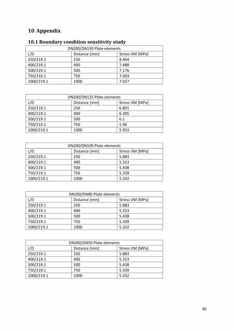
A small study was conducted to find the minimum distance between the junction and the boundary

condition, see Appendix 10.1. It is recommended that the distance between a run/branch pipe

junction and the boundary condition should be at least 7.5√𝑟𝑡 [9]. In this work the only boundary

conditions that will be considered can be seen in Figure 2. In real life application, the branch

connection of interest is rarely that small. In the most cases it is connected to a large piping system.

This means that the user of this method needs to extract the stresses from CAEPIPE, which are

highlighted in Figure 11, then transfer them to FEA.

Figure 11, CAEPIPE displaying reaction forces for each node on a branch connection.

In Figure 11 the branch pipe is located between node 20 and 40, which means that equation 10

calculates the out-of-plane SIF and equation 6 calculates the section modulus for the nozzle. The

other nodes use the same equation 10 to calculate out-of-plane SIF. However, equation 3 is used to

calculate the section modulus for a general pipe instead equation 6 that was used for the nozzle.

The dotted rectangle in the right table of Figure 11 indicates the location of the highest stress (12.19

MPa) caused by the load of 1000 N. The user only needs to find the element which is subjected to the

highest load, in this case it is the pipe element nr 3, which is marked with a dotted line. The element

number can be seen to the left of the dotted rectangle in Figure 11. This force, 250 Nm which can be

seen in the dotted rectangle in Figure 11, will later be used as a boundary condition. The force will be

set as a distributed load over the nodes along the edge of the pipe in Autodesk simulation

mechanical. It is recommended to use the setup position B or C seen in Figure 2 [7]. An important

remark is that, when converting loads from CAEPIPE to Autodesk, it is not the magnitude of the

forces which is of importance, but rather the direction of the resultant vector.

18

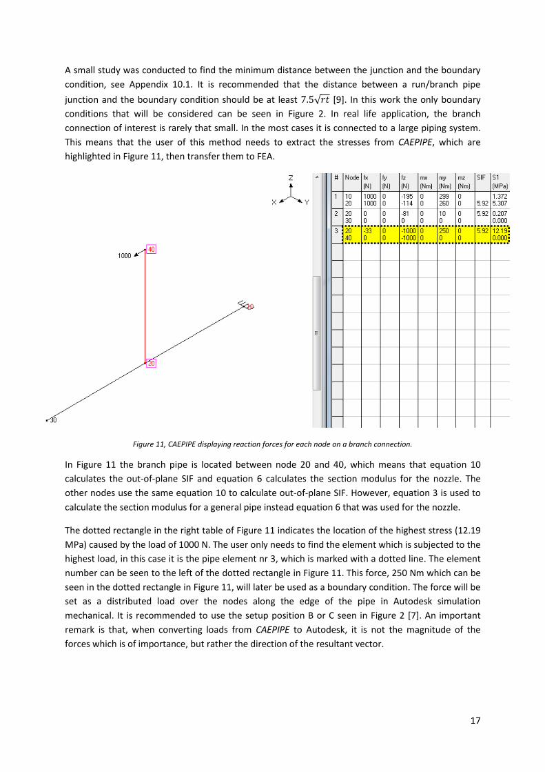
4 Autodesk Simulation Mechanical Autodesk Simulation Mechanical is a commercial FEA software. A free student version is

available from the Autodesk webpage. There is a module in Autodesk called pressure vessel design

(PVD). A simple branch pipe was modeled in PVD. Two different models were made of the setup, one

with solid elements and another with shell elements. They will later be compared in both efficiency

and accuracy. The solid and shell model can be seen in Figure 12.

Figure 12, Two branch connection, solid elements to the left and shell elements to the right

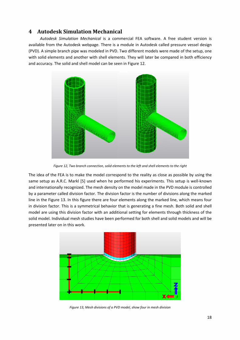
The idea of the FEA is to make the model correspond to the reality as close as possible by using the

same setup as A.R.C. Markl [5] used when he performed his experiments. This setup is well-known

and internationally recognized. The mesh density on the model made in the PVD module is controlled

by a parameter called division factor. The division factor is the number of divisions along the marked

line in the Figure 13. In this figure there are four elements along the marked line, which means four

in division factor. This is a symmetrical behavior that is generating a fine mesh. Both solid and shell

model are using this division factor with an additional setting for elements through thickness of the

solid model. Individual mesh studies have been performed for both shell and solid models and will be

presented later on in this work.

Figure 13, Mesh divisions of a PVD model, show four in mesh division

19

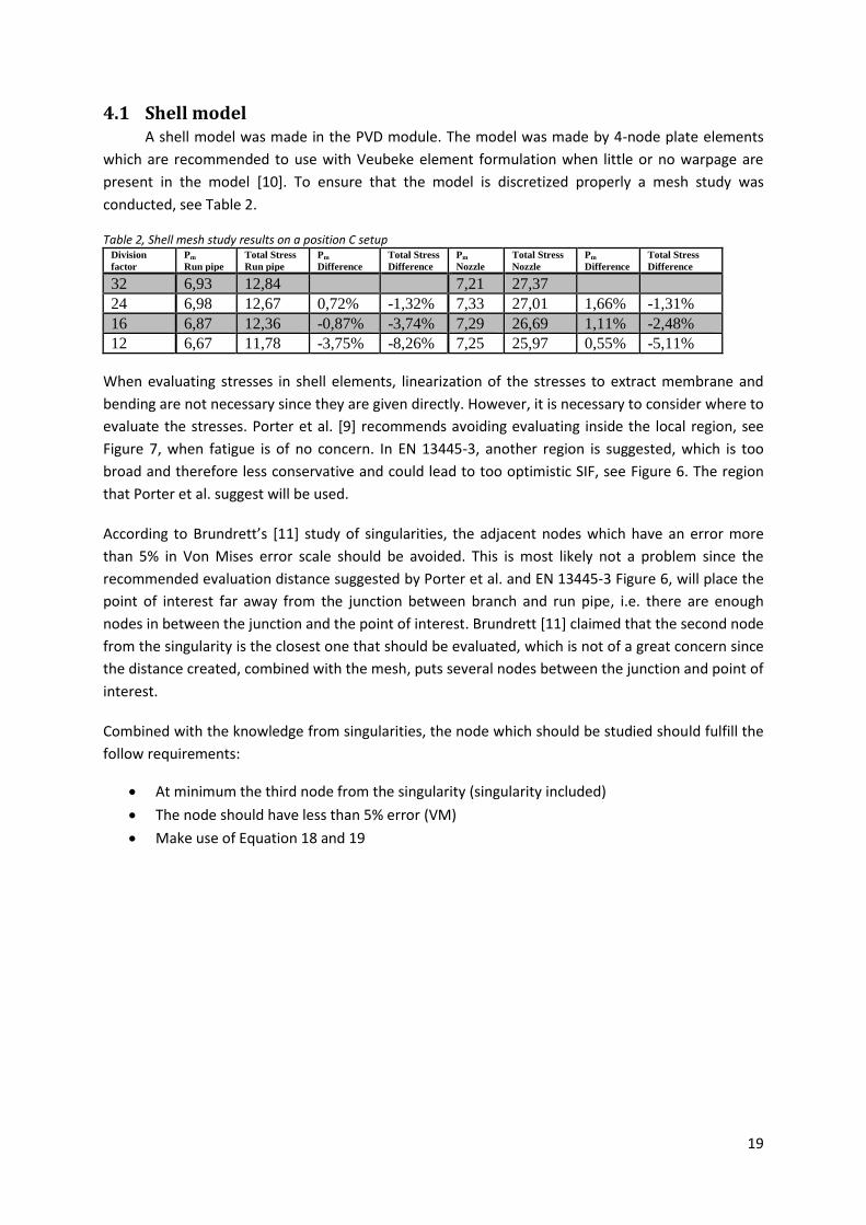
4.1 Shell model A shell model was made in the PVD module. The model was made by 4-node plate elements

which are recommended to use with Veubeke element formulation when little or no warpage are

present in the model [10]. To ensure that the model is discretized properly a mesh study was

conducted, see Table 2.

Table 2, Shell mesh study results on a position C setup Division

factor

Pm

Run pipe

Total Stress

Run pipe

Pm

Difference

Total Stress

Difference

Pm

Nozzle

Total Stress

Nozzle

Pm

Difference

Total Stress

Difference

32 6,93 12,84 7,21 27,37

24 6,98 12,67 0,72% -1,32% 7,33 27,01 1,66% -1,31%

16 6,87 12,36 -0,87% -3,74% 7,29 26,69 1,11% -2,48%

12 6,67 11,78 -3,75% -8,26% 7,25 25,97 0,55% -5,11%

When evaluating stresses in shell elements, linearization of the stresses to extract membrane and

bending are not necessary since they are given directly. However, it is necessary to consider where to

evaluate the stresses. Porter et al. [9] recommends avoiding evaluating inside the local region, see

Figure 7, when fatigue is of no concern. In EN 13445-3, another region is suggested, which is too

broad and therefore less conservative and could lead to too optimistic SIF, see Figure 6. The region

that Porter et al. suggest will be used.

According to Brundrett’s [11] study of singularities, the adjacent nodes which have an error more

than 5% in Von Mises error scale should be avoided. This is most likely not a problem since the

recommended evaluation distance suggested by Porter et al. and EN 13445-3 Figure 6, will place the

point of interest far away from the junction between branch and run pipe, i.e. there are enough

nodes in between the junction and the point of interest. Brundrett [11] claimed that the second node

from the singularity is the closest one that should be evaluated, which is not of a great concern since

the distance created, combined with the mesh, puts several nodes between the junction and point of

interest.

Combined with the knowledge from singularities, the node which should be studied should fulfill the

follow requirements:

At minimum the third node from the singularity (singularity included)

The node should have less than 5% error (VM)

Make use of Equation 18 and 19

20

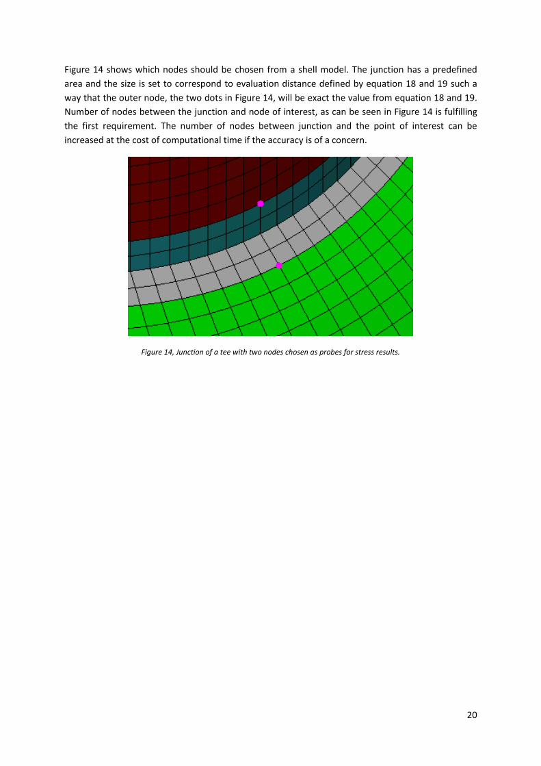
Figure 14 shows which nodes should be chosen from a shell model. The junction has a predefined

area and the size is set to correspond to evaluation distance defined by equation 18 and 19 such a

way that the outer node, the two dots in Figure 14, will be exact the value from equation 18 and 19.

Number of nodes between the junction and node of interest, as can be seen in Figure 14 is fulfilling

the first requirement. The number of nodes between junction and the point of interest can be

increased at the cost of computational time if the accuracy is of a concern.

Figure 14, Junction of a tee with two nodes chosen as probes for stress results.

21

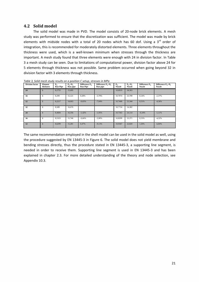
4.2 Solid model The solid model was made in PVD. The model consists of 20-node brick elements. A mesh

study was performed to ensure that the discretization was sufficient. The model was made by brick

elements with midside nodes with a total of 20 nodes which has 60 dof. Using a 3rd order of

integration, this is recommended for moderately distorted elements. Three elements throughout the

thickness were used, which is a well-known minimum when stresses through the thickness are

important. A mesh study found that three elements were enough with 24 in division factor. In Table

3 a mesh study can be seen. Due to limitations of computational power, division factor above 24 for

5 elements through thickness was not possible. Same problem occurred when going beyond 32 in

division factor with 3 elements through thickness.

Table 3, Solid mesh study results on a position C setup, stresses in MPa Division factor Element

thickness

Pm

Run Pipe

Pm+Pb

Run pipe

Difference Pm

Run Pipe

Difference Pm+Pb

Run pipe

Pm

Nozzle

Pm+Pb

Nozzle

Difference Pm

Nozzle

Difference Pm+Pb

Nozzle

24 5 8,2755 15,695 10,6919 24,363

16 5 8,299 15,121 0,28% -3,79% 10,7074 23,799 0,14% -2,37%

12 5 8,2217 14,663 -0,65% -7,04% 10,7468 23,344 0,51% -4,36%

32 3 8,589 16,676 10,7724 24,382

24 3 8,4684 16,356 -1,42% -1,95% 10,7363 24,114 -0,34% -1,11%

16 3 8,5323 15,746 -0,66% -5,90% 10,8299 23,371 0,53% -4,32%

12 3 8,6299 15,281 0,47% -9,13% 10,9367 22,820 1,50% -6,84%

The same recommendation employed in the shell model can be used in the solid model as well, using

the procedure suggested by EN 13445-3 in Figure 6. The solid model does not yield membrane and

bending stresses directly, thus the procedure stated in EN 13445-3, a supporting line segment, is

needed in order to receive them. Supporting line segment is used in EN 13445-3 and has been

explained in chapter 2.3. For more detailed understanding of the theory and node selection, see

Appendix 10.3.

22

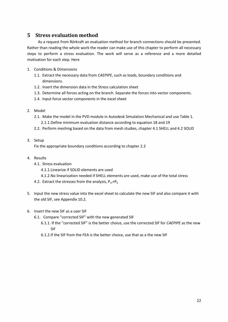
5 Stress evaluation method As a request from Rörkraft an evaluation method for branch connections should be presented.

Rather than reading the whole work the reader can make use of this chapter to perform all necessary

steps to perform a stress evaluation. The work will serve as a reference and a more detailed

motivation for each step. Here

1. Conditions & Dimensions

1.1. Extract the necessary data from CAEPIPE, such as loads, boundary conditions and

dimensions.

1.2. Insert the dimension data in the Stress calculation sheet

1.3. Determine all forces acting on the branch. Separate the forces into vector components.

1.4. Input force vector components in the excel sheet

2. Model

2.1. Make the model in the PVD module in Autodesk Simulation Mechanical and use Table 1.

2.1.1. Define minimum evaluation distance according to equation 18 and 19

2.2. Perform meshing based on the data from mesh studies, chapter 4.1 SHELL and 4.2 SOLID

3. Setup

Fix the appropriate boundary conditions according to chapter 2.2

4. Results

4.1. Stress evaluation

4.1.1. Linearize if SOLID elements are used

4.1.2. No linearization needed if SHELL elements are used, make use of the total stress

4.2. Extract the stresses from the analysis, Pm+Pb

5. Input the new stress value into the excel sheet to calculate the new SIF and also compare it with

the old SIF, see Appendix 10.2.

6. Insert the new SIF as a user SIF

6.1. Compare “corrected SIF” with the new generated SIF

6.1.1. If the “corrected SIF” is the better choice, use the corrected SIF for CAEPIPE as the new

SIF

6.1.2. If the SIF from the FEA is the better choice, use that as a the new SIF

23

6 Results In this section the results from a number of simulations will be presented. Stresses from a solid

model will be compared to stresses from a shell model. Three different results will be presented from

a single example case, calculated with three different methods; one as a standard CAEPIPE case with

EN 13480-3, one with the corrected SIF according to EN 13480-3 and one employing the method

presented in this work.

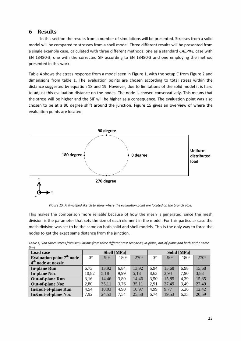
Table 4 shows the stress response from a model seen in Figure 1, with the setup C from Figure 2 and

dimensions from table 1. The evaluation points are chosen according to total stress within the

distance suggested by equation 18 and 19. However, due to limitations of the solid model it is hard

to adjust this evaluation distance on the nodes. The node is chosen conservatively. This means that

the stress will be higher and the SIF will be higher as a consequence. The evaluation point was also

chosen to be at a 90 degree shift around the junction. Figure 15 gives an overview of where the

evaluation points are located.

Figure 15, A simplified sketch to show where the evaluation point are located on the branch pipe.

This makes the comparison more reliable because of how the mesh is generated, since the mesh

division is the parameter that sets the size of each element in the model. For this particular case the

mesh division was set to be the same on both solid and shell models. This is the only way to force the

nodes to get the exact same distance from the junction.

Table 4, Von Mises stress from simulations from three different test scenarios, in-plane, out-of-plane and both at the same time

Load case Shell [MPa] Solid [MPa]

Evaluation point 7th

node

4th

node at nozzle

0° 90° 180° 270° 0° 90° 180° 270°

In-plane Run

In-plane Noz

6,73

10,82

13,92

5,18

6,84

9,99

13,92

5,18

6,94

8,63

15,68

3,94

6,98

7,90

15,68

3,83

Out-of-plane Run

Out-of-plane Noz

3,16

2,80

14,46

35,11

3,80

3,76

14,46

35,11

3,50

2,91

15,85

27,49

4,39

3,49

15,85

27,49

In&out-of-plane Run

In&out-of-plane Noz

4,54

7,92

10,03

24,53

4,90

7,54

10,97

25,58

4,99

6,74

9,77

19,53

5,26

6,33

12,42

20,59

24

From Table 4 it is noted that the solid model and the shell model similar stresses with some

deviation. However, the deviation is not that great. A significant increase in the deviation can be seen

in 90 and 180 degree evaluation point. In Table 4 a more distinct deviation in shell and solid values at

90 and 270 degrees can be seen. They are also connected to out-of-plane load. This is due to the

deformation that occurs at that specific location. This is most likely because the shell model cannot

properly process the high bending stress that occurs at that location compared to the solid model.

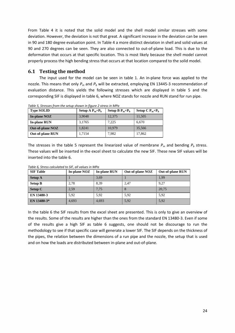
6.1 Testing the method The input used for the model can be seen in table 1. An in-plane force was applied to the

nozzle. This means that only Pm and Pb will be extracted, employing EN 13445-3 recommendation of

evaluation distance. This yields the following stresses which are displayed in table 5 and the

corresponding SIF is displayed in table 6, where NOZ stands for nozzle and RUN stand for run pipe.

Table 5, Stresses from the setup shown in figure 2 stress in MPa

Type SOLID Setup A Pm+Pb Setup B Pm+Pb Setup C Pm+Pb

In-plane NOZ 3,9048 12,375 11,505

In-plane RUN 3,1765 7,225 6,670

Out-of-plane NOZ 1,8241 10,979 35,566

Out-of-plane RUN 1,7154 7,982 17,862

The stresses in the table 5 represent the linearized value of membrane Pm and bending Pb stress.

These values will be inserted in the excel sheet to calculate the new SIF. These new SIF values will be

inserted into the table 6.

Table 6, Stress calculated to SIF, all values in MPa

SIF Table In-plane NOZ In-plane RUN Out-of-plane NOZ Out-of-plane RUN

Setup A 1 3,69 1 1,99

Setup B 2,78 8,39 2,47 9,27

Setup C 2,59 7,75 8 20,75

EN 13480-3 5,92 5,92 5,92 5,92

EN 13480-3* 4,693 4,693 5,92 5,92

In the table 6 the SIF results from the excel sheet are presented. This is only to give an overview of

the results. Some of the results are higher than the ones from the standard EN 13480-3. Even if some

of the results give a high SIF as table 6 suggests, one should not be discourage to run the

methodology to see if that specific case will generate a lower SIF. The SIF depends on the thickness of

the pipes, the relation between the dimensions of a run pipe and the nozzle, the setup that is used

and on how the loads are distributed between in-plane and out-of-plane.

25

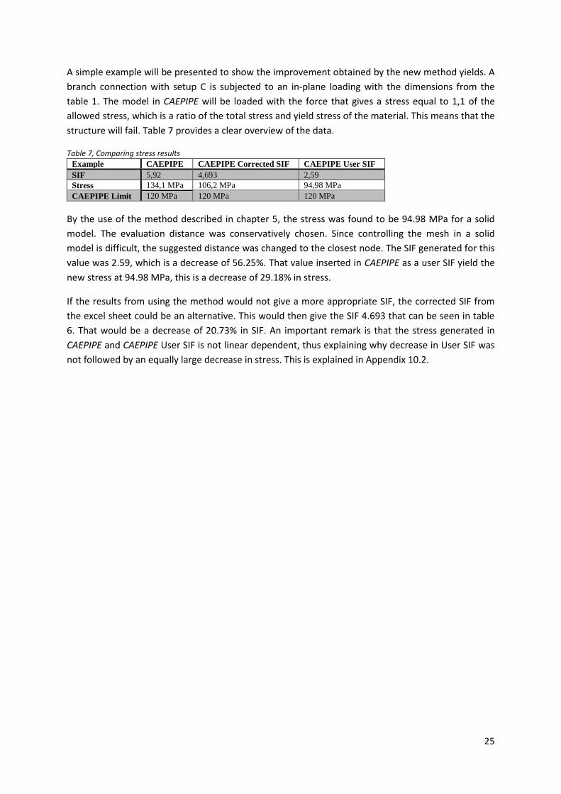
A simple example will be presented to show the improvement obtained by the new method yields. A

branch connection with setup C is subjected to an in-plane loading with the dimensions from the

table 1. The model in CAEPIPE will be loaded with the force that gives a stress equal to 1,1 of the

allowed stress, which is a ratio of the total stress and yield stress of the material. This means that the

structure will fail. Table 7 provides a clear overview of the data.

Table 7, Comparing stress results

Example CAEPIPE CAEPIPE Corrected SIF CAEPIPE User SIF

SIF 5,92 4,693 2,59

Stress 134,1 MPa 106,2 MPa 94,98 MPa

CAEPIPE Limit 120 MPa 120 MPa 120 MPa

By the use of the method described in chapter 5, the stress was found to be 94.98 MPa for a solid

model. The evaluation distance was conservatively chosen. Since controlling the mesh in a solid

model is difficult, the suggested distance was changed to the closest node. The SIF generated for this

value was 2.59, which is a decrease of 56.25%. That value inserted in CAEPIPE as a user SIF yield the

new stress at 94.98 MPa, this is a decrease of 29.18% in stress.

If the results from using the method would not give a more appropriate SIF, the corrected SIF from

the excel sheet could be an alternative. This would then give the SIF 4.693 that can be seen in table

6. That would be a decrease of 20.73% in SIF. An important remark is that the stress generated in

CAEPIPE and CAEPIPE User SIF is not linear dependent, thus explaining why decrease in User SIF was

not followed by an equally large decrease in stress. This is explained in Appendix 10.2.

26

7 Discussion The stress evaluation method which has been presented in this work is based on EN 13445-3,

ASME directives and articles. The main focus has been on the standards EN 13480-3 and EN 13445-3,

since Rörkraft is using those standards and they are also the most known and used in European

piping industry.

The common way to determine the Stress Intensity Factor is through a fatigue test and an S-N curve.

However, as it was stated in the earlier chapters, this procedure will not be used, due to the amount

of resources an experimental test requires. As explained in chapter 2.2, the SIF is the factor between

a butt weld with 1 in SIF and a branch connection. In order to proceed with this work, the following

limitations were necessary:

When considering all these restrictions, the behavior of the model will only be dependent on a small

set of parameters. The two most important parameters are the loading condition acting on the

model and the dimensions of the model. The advantage of only having few changing parameters is

that it will make it easier to create a methodology for stress evaluation. Another advantage is that

the risk of error will be significantly decreased. This method minimizes these dangerous errors or

removes them completely by giving clear instructions on how and where to evaluate the specific

branch connection.

Of course, the question is raised if the stress evaluation method developed in this work is

appropriate and applicable. Experimental tests could not be performed due to the lack of funding

and any other data which could validate the methodology could not be found. Due to this limitation,

I have chosen to use standard EN 13445-3 and Porter’s report to validate this work. By doing so, I can

claim that the methodology is sufficient because all the recommendations have been followed.

In FE-solid model a finer mesh could improve the accuracy, however, it is with only a few percent and

due to limitations with computational power, and the level of accuracy was considered to be

sufficient according to table 3. By more computational power, the number of nodes between the

singularity and the node of interest could be increased and thus the accuracy could be improved. The

size of the Von Mises error is below 5% and it is considered to be acceptable.

At an early stage of this work I considered including a weld into my model, however both of my

advisors recommended to avoid including a weld due to its complexity. There were also other

reasons why the weld was omitted in this work. The software that was used, PVD module in

Autodesk, does not allow the user to specify any weld. When performing a static analysis one does

not evaluate the local region (where the weld resides), only when fatigue is of concern according to

EN 13445-3. However if the weld was included there would be some stress relaxations at the junction

and the singularity would be removed. This would also lead to a greater accuracy of the model and

provide a deeper understanding of where and how the SIF affects branch connections. Including the

weld would produce a model and stress results which are closer to reality. This could be a

consideration for future studies on this subject.

27

Comparing tables 4 and 5, one can see that the stress results are consistently lower for the solid

model compared to the shell model. This is most likely related to the element formulation, where

solids are better to use when the area of interest has sharp corners. Bending stresses that reside

close to a sharp corner have a greater influence on the shell model compared to the solid model.

The meshing procedure in Autodesk Simulation Mechanical in Pressure Vessel Design module is very

limited, because one cannot change the structure of the mesh, especially in the solid model. It is very

difficult to adjust the nodes and create specific evaluation points in the mesh when using the PVD

module. Because of the limited meshing options, the evaluation procedure becomes more difficult

and some simplifications have to be made. A more conservative point has to be chosen, because the

meshing imposed some limitations. Porter et al. [9] report suggests a shorter evaluation distance

from the junction compared to what EN 13445-3 suggests. This would lead to higher stresses and a

higher SIF. The evaluation distance that Porter suggests is chosen because it explicitly states that the

peak stresses are not included into the evaluation. The European standard, however, excludes wider

region, which includes not solely the peak stresses, but other local stresses as well, which is not

desired. In short, this means that the region suggested in the European standard would be too large

and the stress results would be too optimistic.

The solid mesh came to be unnecessary large where it was not needed, due to how mesh divisions

are defined in the PVD module. At the edges of the model, where no stress evaluation takes place,

the elements were unnecessarily small. If the meshing procedure was not so limited, the mesh could

be significantly improved from a computational aspect. If it were possible to make the mesh coarse

at the boundary conditions, the computational time would be reduced. A coarser mesh far away

from the connection would not influence the result, since the force and the clamped side is

considered to be far away according to the mesh sensitivity study. The point of interest is the

junction between the run pipe and the branch pipe. The European standard and Porter’s report

provide us with a concrete number for evaluation distance. This distance has to correspond to a node

in the mesh, but a node is not always present at a given distance. If there is no node at this location,

the closest node towards the junction will be chosen.

The linearization procedure stated that the supporting line segment should be perpendicular towards

the surface. This was not possible in all situations. The user has to be careful when selecting the

nodes to define the supporting line segment. The alignment of the elements is not completely

uniform throughout the thickness, especially in the run pipe around the junction at the sides. If the

deviation from perpendicularity is too great, the stresses will be lower, mostly because the bending

stresses will not be fully represented. At the branch pipe the mesh generation is not a big problem

because of how the elements are aligned. However, at the run pipe at some locations, the mesh can

be formed in a way that perpendicular supporting line segments are not possible. Some deviations

are unavoidable. This problem does not exist for the shell model.

Although it is not investigated in this work, this method could be used to assist the user in making an

evaluation of stress limits as Figure 5 and EN 13445-3 suggests. The evaluation distance can be used

as a limiter for stresses close to the junction. The references in this work provide more detailed

explanation of how such procedure should be performed.

28

8 Conclusion A methodology for evaluation of the Stress Intensity Factor in pipe branch connections has

been developed in this work. It consists of a background of the necessary theory, which presents

information of the SIF and how it is calculated. This work thoroughly explains how a model should be

made in order to achieve accurate and reliable results. Data from results are presented to illustrate

how much of an improvement can be made by using this methodology. An excel calculation sheet

has been designed in order to simplify the necessary calculations.

The results show that an improvement can be made. The example that is presented in the results,

demonstrates a reduction of the stresses up to 30 % for an in-plane load. For the cases when the

methodology cannot improve the SIF, the excel sheet will provide an alternative way of calculating

the SIF, which is called the corrected SIF. The corrected SIF follows EN 13480-3. With the corrected

SIF the stresses could be lowered up to 20% for an in-plane.

Use of the shell model is the most desirable due to the accuracy compared to efficiency and how

user friendly it is. With PVD the shell model is incredibly easy to setup and one can define the area of

vicinity within the mesh function in such a way that the node of interest will be at the desired

evaluation distance stated in chapter 2.3. From a computational aspect the shell model is faster and

less demanding to the hardware. We are not including a singularity in any evaluation method and if

the accuracy is of concern one can add more nodes between the singularity and the node of interest

in the model. The shell model does not need any linearization since the stresses are presented

directly.

Table 4 illustrates stress results for the shell model. From these results it is clear that the shell model

gives higher stresses than the solid model. Therefore the shell model is good candidate for quick

evaluation procedure when accuracy is not of importance. The shell model can be considered to be

safer since it will give higher SIF than the solid model, thus making it more conservative. If one has

the need and time to extract a more accurate value, the solid model is a better choice.

For inexperienced users the shell model is recommended due to its simplicity. It is conservative and

easy to setup. If a user is experienced, knowledgeable and has the resources, the solid model is

recommended.

29

9 References [1] European standard EN 13480-3:2012. Metallic Industrial Piping - Part 3: Design and Calculation,

Swedish Standard Institute, Stockholm, 2012

[2] CAEPIPE. SST Systems, Inc., San Jose, USA, 2013. Software available at http://www.sstusa.com/

last used 2014-11-15

[3] European standard EN 13445-3:2009+C4:2012. Unfired pressure vessels, Swedish Standard

Institute, Stockholm, 2012

[4] Autodesk Simulation Mechanical. Autodesk, Inc., San Rafael, USA, 2014. Software available at

http://www.autodesk.com/ last used 2014-11-15

[5] A.R.C. Markl. Piping-Flexibility Analysis. Transactions of the ASME, 77:127-149, 1955.

[6] What is a Stress Intensification Factor (SIF)? Paulin research group, 2008. Available at

http://www.paulin.com/web_sifandfesif.aspx

[7] R. Carter. Background of SIFs and Stress Induces for Moment Loadings of Piping Components.

Electric power research institute, Palo Alto, 2005.

[8] C. Hinnant and T. Paulin. Experimental Evaluation of the Markl Fatigue Methods and ASME piping

Stress Intensification Factors. ASME 2008 Pressure Vessels and Piping Conference, Chicago, 2008.

[9] M. Porter, D. Martens and S. M. Cauldwell. A Suggested Evaluation Procedure for Shell/Plate

Element Finite Element Nozzle Models. ASME Pressure Vessels and Piping, 388, 1999.

[10] Autodesk simulation mechanical 2014: help. Plate Elements. Available at

http://help.autodesk.com/view/ASMECH/2014/ENU/?guid=GUID-2566D867-68F5-4154-9297-

F4B93BCE625D last used 2014-05-14.

[11] Mesh Refinements Near Discontinuities, 2013. Available at

http://www.pveng.com/FEA/FEANotes/RefineNearDiscon/RefineNearDiscon.php last used 2014-05-

14

[12] J. L. Hechmer and G.L. Hollinger.Three-Dimensional Stress Criteria – Summary of the PVRC

Project. ASME Journal of Pressure Vessel Technology, 122:105-109, 2000.

[13] Autodesk simulation mechanical 2014: help. How to calculate Pm and Pm Pb. Available. at

http://help.autodesk.com/view/ASMECH/2014/ENU/?guid=GUID-301D1FD3-CBB2-4F4D-BCF8-

76BF098A5B73 last used 2014-05-14

30

10 Appendix

10.1 Boundary condition sensitivity study DN200/DN150 Plate elements

L/D Distance [mm] Stress VM [MPa]

250/219.1 250 8.464

400/219.1 400 7.488

500/219.1 500 7.176

750/219.1 750 7.003

1000/219.1 1000 7.027

DN200/DN125 Plate elements

L/D Distance [mm] Stress VM [MPa]

250/219.1 250 6.891

400/219.1 400 6.305

500/219.1 500 6.1

750/219.1 750 5.96

1000/219.1 1000 5.953

DN200/DN100 Plate elements

L/D Distance [mm] Stress VM [MPa]

250/219.1 250 5.883

400/219.1 400 5.553

500/219.1 500 5.438

750/219.1 750 5.339

1000/219.1 1000 5.332

DN200/DN80 Plate elements

L/D Distance [mm] Stress VM [MPa]

250/219.1 250 5.883

400/219.1 400 5.553

500/219.1 500 5.438

750/219.1 750 5.339

1000/219.1 1000 5.332

DN200/DN50 Plate elements

L/D Distance [mm] Stress VM [MPa]

250/219.1 250 5.883

400/219.1 400 5.553

500/219.1 500 5.438

750/219.1 750 5.339

1000/219.1 1000 5.332

31

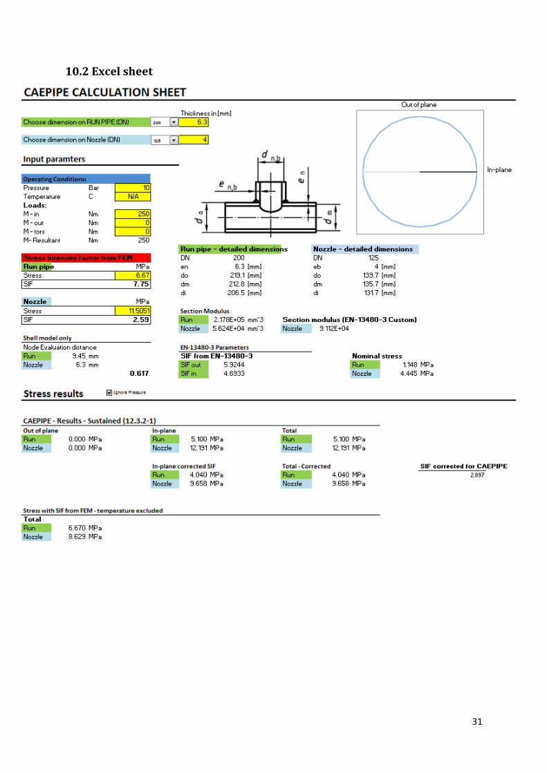
10.2 Excel sheet

32

10.2.1 Stress calculation sheet

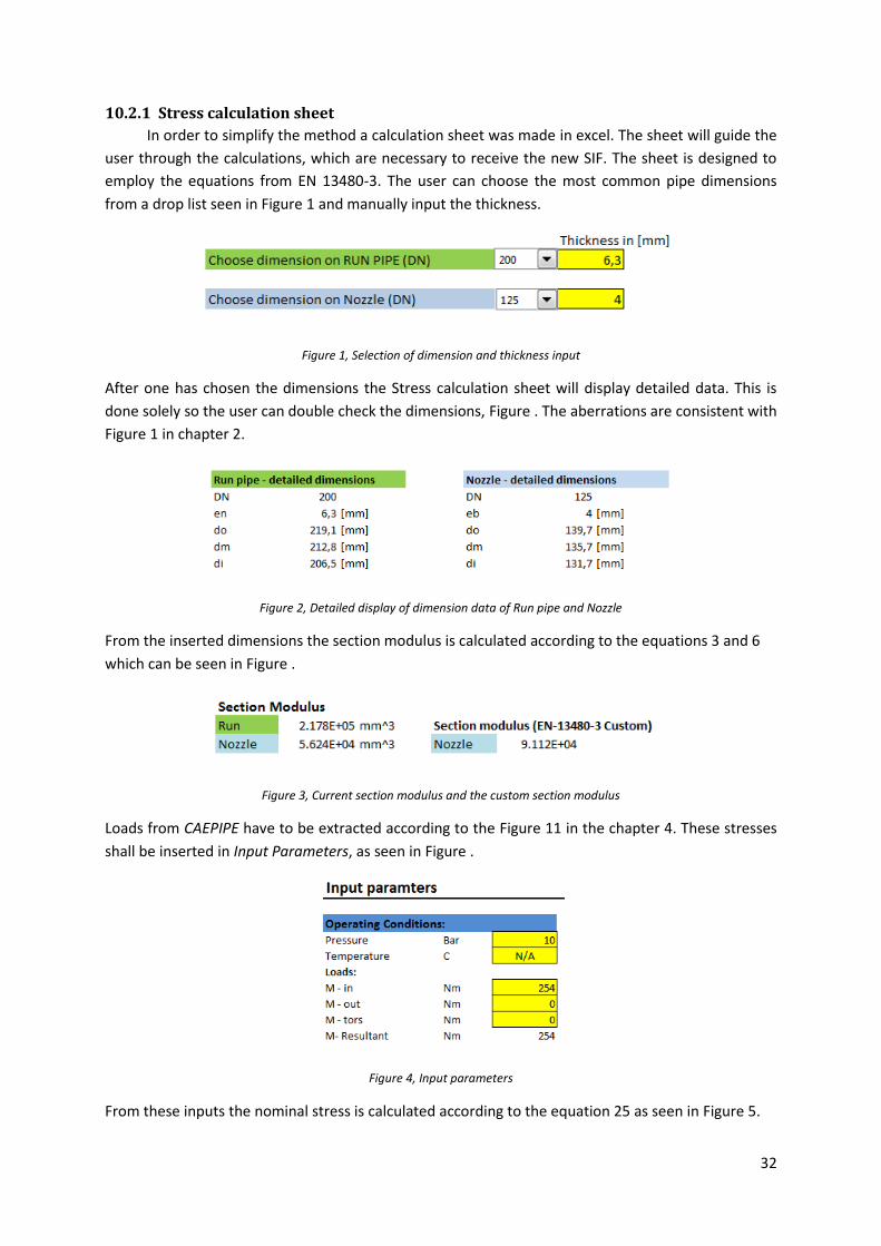
In order to simplify the method a calculation sheet was made in excel. The sheet will guide the

user through the calculations, which are necessary to receive the new SIF. The sheet is designed to

employ the equations from EN 13480-3. The user can choose the most common pipe dimensions

from a drop list seen in Figure 1 and manually input the thickness.

Figure 1, Selection of dimension and thickness input

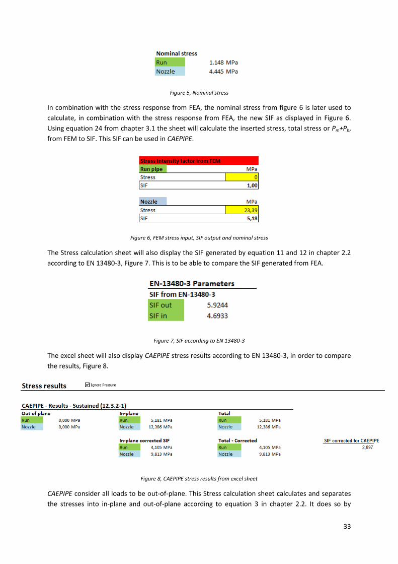
After one has chosen the dimensions the Stress calculation sheet will display detailed data. This is

done solely so the user can double check the dimensions, Figure . The aberrations are consistent with

Figure 1 in chapter 2.

Figure 2, Detailed display of dimension data of Run pipe and Nozzle

From the inserted dimensions the section modulus is calculated according to the equations 3 and 6

which can be seen in Figure .

Figure 3, Current section modulus and the custom section modulus

Loads from CAEPIPE have to be extracted according to the Figure 11 in the chapter 4. These stresses

shall be inserted in Input Parameters, as seen in Figure .

Figure 4, Input parameters

From these inputs the nominal stress is calculated according to the equation 25 as seen in Figure 5.

33

Figure 5, Nominal stress

In combination with the stress response from FEA, the nominal stress from figure 6 is later used to

calculate, in combination with the stress response from FEA, the new SIF as displayed in Figure 6.

Using equation 24 from chapter 3.1 the sheet will calculate the inserted stress, total stress or Pm+Pb,

from FEM to SIF. This SIF can be used in CAEPIPE.

Figure 6, FEM stress input, SIF output and nominal stress

The Stress calculation sheet will also display the SIF generated by equation 11 and 12 in chapter 2.2

according to EN 13480-3, Figure 7. This is to be able to compare the SIF generated from FEA.

Figure 7, SIF according to EN 13480-3

The excel sheet will also display CAEPIPE stress results according to EN 13480-3, in order to compare

the results, Figure 8.

Figure 8, CAEPIPE stress results from excel sheet

CAEPIPE consider all loads to be out-of-plane. This Stress calculation sheet calculates and separates

the stresses into in-plane and out-of-plane according to equation 3 in chapter 2.2. It does so by

34

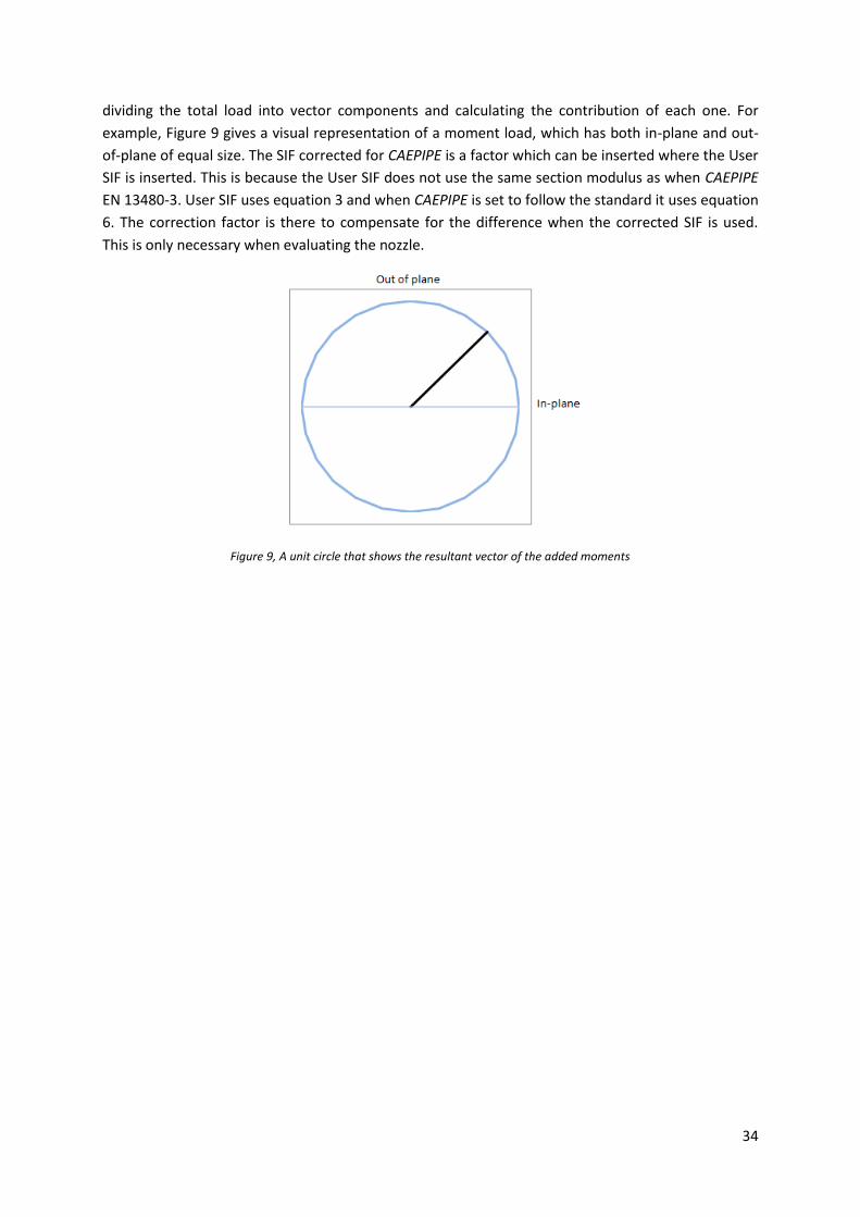
dividing the total load into vector components and calculating the contribution of each one. For

example, Figure 9 gives a visual representation of a moment load, which has both in-plane and out-

of-plane of equal size. The SIF corrected for CAEPIPE is a factor which can be inserted where the User

SIF is inserted. This is because the User SIF does not use the same section modulus as when CAEPIPE

EN 13480-3. User SIF uses equation 3 and when CAEPIPE is set to follow the standard it uses equation

6. The correction factor is there to compensate for the difference when the corrected SIF is used.

This is only necessary when evaluating the nozzle.

Figure 9, A unit circle that shows the resultant vector of the added moments

35

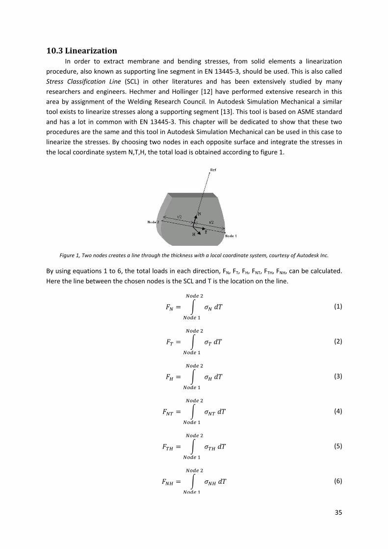
10.3 Linearization In order to extract membrane and bending stresses, from solid elements a linearization

procedure, also known as supporting line segment in EN 13445-3, should be used. This is also called

Stress Classification Line (SCL) in other literatures and has been extensively studied by many

researchers and engineers. Hechmer and Hollinger [12] have performed extensive research in this

area by assignment of the Welding Research Council. In Autodesk Simulation Mechanical a similar

tool exists to linearize stresses along a supporting segment [13]. This tool is based on ASME standard

and has a lot in common with EN 13445-3. This chapter will be dedicated to show that these two

procedures are the same and this tool in Autodesk Simulation Mechanical can be used in this case to

linearize the stresses. By choosing two nodes in each opposite surface and integrate the stresses in

the local coordinate system N,T,H, the total load is obtained according to figure 1.

Figure 1, Two nodes creates a line through the thickness with a local coordinate system, courtesy of Autodesk Inc.

By using equations 1 to 6, the total loads in each direction, FN, FT, FH, FNT, FTH, FNH, can be calculated.

Here the line between the chosen nodes is the SCL and T is the location on the line.

𝐹𝑁 = ∫ 𝜎𝑁 𝑑𝑇

𝑁𝑜𝑑𝑒 2

𝑁𝑜𝑑𝑒 1

(1)

𝐹𝑇 = ∫ 𝜎𝑇 𝑑𝑇

𝑁𝑜𝑑𝑒 2

𝑁𝑜𝑑𝑒 1

(2)

𝐹𝐻 = ∫ 𝜎𝐻 𝑑𝑇

𝑁𝑜𝑑𝑒 2

𝑁𝑜𝑑𝑒 1

(3)

𝐹𝑁𝑇 = ∫ 𝜎𝑁𝑇 𝑑𝑇

𝑁𝑜𝑑𝑒 2

𝑁𝑜𝑑𝑒 1

(4)

𝐹𝑇𝐻 = ∫ 𝜎𝑇𝐻 𝑑𝑇

𝑁𝑜𝑑𝑒 2

𝑁𝑜𝑑𝑒 1

(5)

𝐹𝑁𝐻 = ∫ 𝜎𝑁𝐻 𝑑𝑇

𝑁𝑜𝑑𝑒 2

𝑁𝑜𝑑𝑒 1

(6)

36

After the total loads have been calculated, it is now possible to calculate the membrane stress for all

six components. The length of the SCL is t.

𝜎𝑁

𝑀 =𝐹𝑁

𝑡

(7)

𝜎𝑇

𝑀 =𝐹𝑇

𝑡

(8)

𝜎𝐻

𝑀 =𝐹𝐻

𝑡

(9)

𝜏𝑁𝑇

𝑀 =𝐹𝑁𝑇

𝑡

(10)

𝜏𝑇𝐻𝑀 =

𝐹𝑇𝐻

𝑡

(11)

𝜏𝑁𝐻

𝑀 =𝐹𝑁𝐻

𝑡

(12)

From the previous stated equations 7 to 12 the principal stresses can be derived. Next step is to find

the bending stresses. We only need the two components which are perpendicular to the SCL.

𝑀𝑁 = ∫ 𝜎𝑁 𝑇𝑑𝑇

𝑁𝑜𝑑𝑒 2

𝑁𝑜𝑑𝑒 1

(13)

𝑀𝐻 = ∫ 𝜎𝐻 𝑇𝑑𝑇

𝑁𝑜𝑑𝑒 2

𝑁𝑜𝑑𝑒 1

(14)

𝑀𝑁𝐻 = ∫ 𝜏𝑁𝐻 𝑇𝑑𝑇

𝑁𝑜𝑑𝑒 2

𝑁𝑜𝑑𝑒 1

(15)

Bending stress are derived according to equation 16, 17 and 18

𝜎𝑁

𝐵 =6𝑀𝑁

𝑡2

(16)

𝜎𝐻

𝐵 =6𝑀𝐻

𝑡2

(17)

𝜏𝑁𝐻

𝐵 =6𝑀𝑁𝐻

𝑡2

(18)

37

Principal stress at the ends of the SCL can be calculated by using equation 19 to 24.

𝜎𝑁

𝑀+𝐵 = 𝜎𝑁𝑀 + 𝜎𝑁

𝐵 (2𝑇

𝑡)

(19)

𝜎𝑇𝑀+𝐵 = 𝜎𝑇

𝑀

(20)

𝜎𝐻

𝑀+𝐵 = 𝜎𝐻𝑀 + 𝜎𝐻

𝐵 (2𝑇

𝑡)

(21)

𝜏𝑁𝑇𝑀+𝐵 = 𝜏𝑁𝑇

𝑀

(22)

𝜏𝑇𝐻𝑀+𝐵 = 𝜏𝑇𝐻

𝑀

(23)

𝜏𝑁𝐻

𝑀+𝐵 = 𝜏𝑁𝐻𝑀 + 𝜏𝑁𝐻

𝐵 (2𝑇

𝑡)

(24)

Sum and find the largest value according to equation 25 and 26. This must be done twice due to two

different sides and nodes.

𝑚𝑎𝑥 {

|𝑝1𝑀 − 𝑝2

𝑀|

|𝑝2𝑀 − 𝑝3

𝑀|

|𝑝3𝑀 − 𝑝1

𝑀|

(25)

𝑚𝑎𝑥 {

|𝑝1𝑀+𝐵 − 𝑝2

𝑀+𝐵|

|𝑝2𝑀+𝐵 − 𝑝3

𝑀+𝐵|

|𝑝3𝑀+𝐵 − 𝑝1

𝑀+𝐵|

(26)

According to EN 13445-3 Annex C equation C.4.1-1 seen in equation 20 and equation 21 in the work,

the methods stress results from the linearization are applicable.

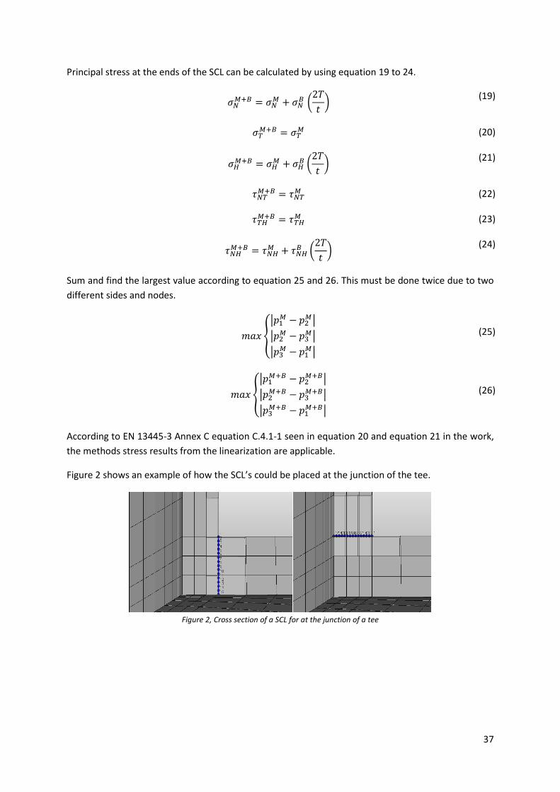
Figure 2 shows an example of how the SCL’s could be placed at the junction of the tee.

Figure 2, Cross section of a SCL for at the junction of a tee