1

Mediterranean Forests in Transition (MEDIT): Deliverable No3

Title: Report on the development/structure/validation of the GREFOS v2 model

Due to Project Month 12, Date: 31/03/2013

Introduction

This manuscript presents the forest dynamics simulation model GREFOS v2. The original version of the

model is a descendant of ForClim (Bugmann and Cramer, 1998; Fyllas et al. 2007). GREFOS v2 builds upon

developments of an earlier version of the model (Fyllas & Troumbis 2009) in addition to the detailed

regeneration algorithm described in Fyllas et al. 2010. It is a model developed to simulate the dynamics of

Mountainous Mediterranean Forest and it specifically parameterised for the dominant tree species found

in Greece and the eastern part of the Mediterranean Basin.

GREFOS is a forest gap dynamics simulator (Botkin et al. 1972; Shugart 1984) and it can be broadly

categorised as an individual-based model (). It simulates the life cycle of each tree in a small stand (usually

900m2: 30x30m) from its birth to its death. Special interest is given to processes of particular importance

like regeneration and growth, and a number of field and laboratory studies have been specifically designed

and used to constrain these model components (Fyllas et al. 2008, Fyllas et al. 2010, Galanidis et al. 2013,

Fyllas et al. 2013).

The new version of the model has been coded in Java and it is available on request from the author. The

following section describes the key model components as summarised in Fig. 1.

Figure 1: Schematic representation of the key model components and their interactions

SLAI, Ii

Climate

Submodel

T, Tx,Tn, P, Ra, RH

Soil Submodel

Θ

Light

Competition

Fire Submodel

ΠFire

Tree Structure

D H = f(D)

FA =

f(D,SLA)

Recruitment

Submodel

2

Model Components

Definition of individual trees

Trees in GREFOS are defined with a diameter based allometry. From the diameter of a tree a set of

architectural parameters is estimated using published equations (Gracia et al 1992, Risch et al. 2005). In

particular given the diameter at breast height (D) the following individual tree characteristics are defined:

Tree height (H: in cm) is given from:

130 1 exp( )H b c D (1), with b and c species specific allometric parameters (Fyllas and Troumbis

2009).

The foliage area (FA: in m2) of a tree is calculated as:

FA SLA D

(2), with ΦΑ and ΦΒ species specific allometric parameters and SLA the specific leaf

area (cm2 g-1) of the species.

The foliage of a tree is assumed to be found at the top (i.e. at height H) defining a circle (flat top canopy)

Climate Submodel

GREFOS simulates climatic processes on a daily timestep. There are two different ways the daily patterns of

temperature (T in oC) and precipitation (P in mm) are generated. The first method reads in daily climate

records from local weather stations. The second method uses a built-in weather generator which generates

daily values of temperature and precipitation from monthly records, assuming a normal probability

distribution for temperature and a log-normal distribution for temperature (Fyllas & Troumbis, 2009).

Daily extraterrestrial radiation (Ra in MJ m-2 d-1) is calculated as (Steduto et al. 2009, Raes et al., 2009):

sin( ) sin( ) cos( ) cos( ) sin( )SCa

K drR

(3)

where Ksc = 118.08 (MJ m-2 d-1) the solar constant, dr the inverse relative distance between the earth and

sun, ω the sunset hour angle, φ the latitude of the plot to simulate and δ the solar declination.

The net shortwave radiation (Rns in MJ m-2 d-1) is given from:

(1 )ns aR a R (4)

where α the canopy albedo taken as constant α=0.23.

The net isothermal longwave radiation (Rnl in MJ m-2 d-1) is calculated by a humidity and cloudiness

corrected version of the Stefan-Boltzmann law:

nl c h KR f f f T (5)

where fc the cloudiness factor, fh the air humidity correction factor, σ the Stefan-Boltzmann constant (4.903

10-9 in MJm-2 K-1 d-1) and

4 4

max min( )2

K KK

T Tf T

(6)

3

with TKmax and TKmin the daily absolute maximum and minimum temperature (K).

The net radiation (Rn) is then calculated as the difference between incoming net shortwave and outgoing

longwave radiation:

n ns nlR R R (7)

The Priestley-Taylor algorithm is used to estimate the daily reference evaporation ETo (MJ m-2 d-1):

0

( )

PT na s R GET

s

(8)

where aPT the Priestley-Taylor coefficient, s (kPa C-1) the slope of the saturation vapor pressure-

temperature relationship, γ (kPa C-1) the psychometric constant and G (MJ m-2 d-1) the soil heat flux.

Soil Submodel and Water Balance

A single layer soil submodel is used in this version of the model in order to run a daily water balance and

estimate a daily soil moisture index (θ).

AW

Z (9), with AW (mm) the soil available water and Z the soil depth (mm).

On a daily timestep AW is computed as:

1t tAW AW P ET Q (10)

Where ET the actual-stand level evapotranspiration transformed to mm and Q (mm) the soil runoff. A

modification to calculate actual evapotranspiration as a function of soil water content has been applied as

described in Flint and Childs (1991).

0SW CET a K ET (11)

Where KC the crop coefficient [Kc=0.7] and αSW the modified Priestley-Taylor coefficient calculated from:

1 exp(B )SWa A (12), with Α=0.916 and B=-9.74, and Θ the relative soil water content calculated

from (Flint and Childs, 1991):

r

s r

(13)

where θr the residual soil water content and θs the water content at saturation. The pedotransfer functions

developed in Wösten et al. (1999, 2001) are used to calculate θr and θs for the van-Genuchten model, by

classifying soils from a coarse to a very fine texture class.

Total stand transpiration (T) and soil evaporation (Es) are estimated from:

canT f ET (14),

SE ET T (15)

4

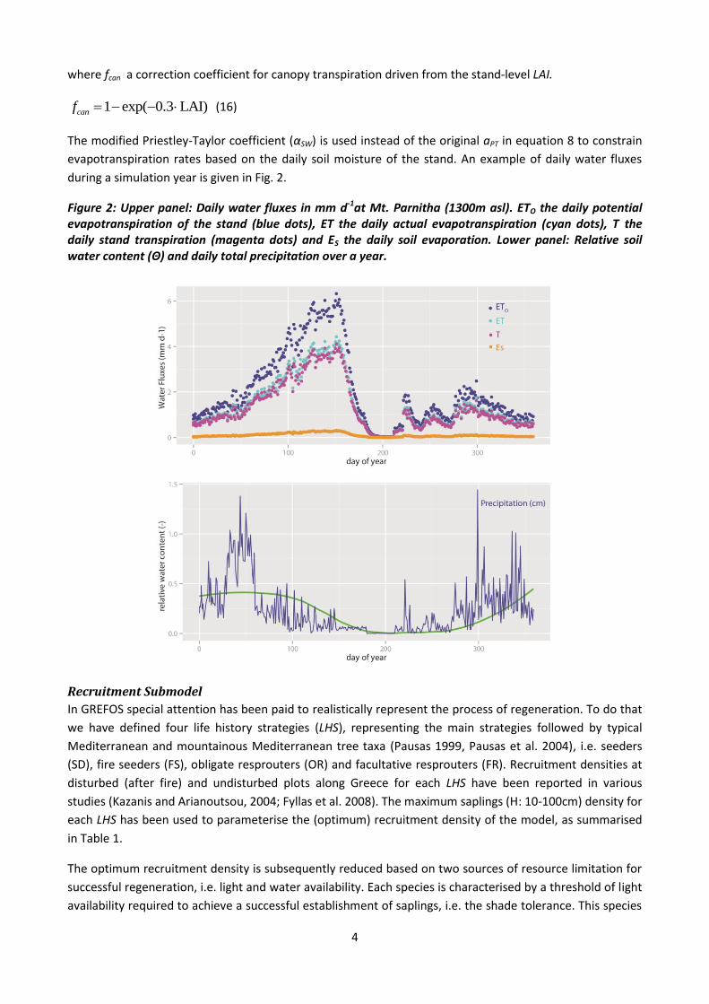
where fcan a correction coefficient for canopy transpiration driven from the stand-level LAI.

1 exp( 0.3 LAI)canf (16)

The modified Priestley-Taylor coefficient (αSW) is used instead of the original aPT in equation 8 to constrain

evapotranspiration rates based on the daily soil moisture of the stand. An example of daily water fluxes

during a simulation year is given in Fig. 2.

Figure 2: Upper panel: Daily water fluxes in mm d-1at Mt. Parnitha (1300m asl). ETO the daily potential evapotranspiration of the stand (blue dots), ET the daily actual evapotranspiration (cyan dots), T the daily stand transpiration (magenta dots) and ES the daily soil evaporation. Lower panel: Relative soil water content (Θ) and daily total precipitation over a year.

Recruitment Submodel

In GREFOS special attention has been paid to realistically represent the process of regeneration. To do that

we have defined four life history strategies (LHS), representing the main strategies followed by typical

Mediterranean and mountainous Mediterranean tree taxa (Pausas 1999, Pausas et al. 2004), i.e. seeders

(SD), fire seeders (FS), obligate resprouters (OR) and facultative resprouters (FR). Recruitment densities at

disturbed (after fire) and undisturbed plots along Greece for each LHS have been reported in various

studies (Kazanis and Arianoutsou, 2004; Fyllas et al. 2008). The maximum saplings (H: 10-100cm) density for

each LHS has been used to parameterise the (optimum) recruitment density of the model, as summarised

in Table 1.

The optimum recruitment density is subsequently reduced based on two sources of resource limitation for

successful regeneration, i.e. light and water availability. Each species is characterised by a threshold of light

availability required to achieve a successful establishment of saplings, i.e. the shade tolerance. This species

5

specific threshold is expressed in GREFOS through a maximum LAI (Leaf Area Index m2 m-2) value above

which saplings of a species cannot establish and thus die. Field measurements of recruitment density and

survivorship along LAI gradients (Fyllas 2007, Fyllas et al. 2008, Politi et al. 2009) are used to estimate the

species specific LAI threshold (LAIT).

Table 1: Life History Strategies used in Grefos and their associated saplings density

Life History Strategy (LHS)

Maximum Saplings Density (saplings m-2)

Typical Species

Fire Seeders (FS) 0.4 // 1.0 (after a fire) P. halepensis, P. brutia

Seeders (SD) 0.4 A. cephalonica, P. nigra

Facultative Resprouters (FR) 0.3 F. sylvatica

Obligate Resprouters (OR) 0.2 Q. coccifera, Q. frainetto

Recruitment is calculated in GREFOS once a year. The optimum number of new saplings provides a source

of new recruits at the age of one year which is added in a pool of available saplings (splPool) for each

species. Saplings are maintained in this pool until the age of 10 years, when they are eventually added as

trees at a specific location. Until that stage saplings do not have specific coordinates, but are rather

considered as a pool of potential recruits. In order for a sapling to increase its age (for example from years

1 to 2) it has to pass the species specific threshold of light availability (LAIT). At each time step light

availability is computed for each member of the saplings pool, by selecting a random location within the

plot and estimating a local leaf area index (LAIL) at a cyclic area of 10 m radius. LAIL is computed as the sum

of foliage area of all established trees within the cyclic area, divided by the area of the circle. No three-

dimensional description of the canopy is pursued, and thus if a mature tree falls within the local cyclic area,

its entire canopy is assumed to shade the target sapling. This algorithm is essentially “scanning” the forest

floor and estimates a level of light availability at random points. If LAIL < LAIT then the target sapling

survives in the current time step. In contrast, with existing gap models, where an aggregated level of

available incoming radiation at the soil surface is estimated, our approach is following a random sampling

procedure which could potentially identify more than one gap within the simulated plot area, and thus lead

to realistic simulations of areas bigger than the gap scale (Fyllas et al., 2010).

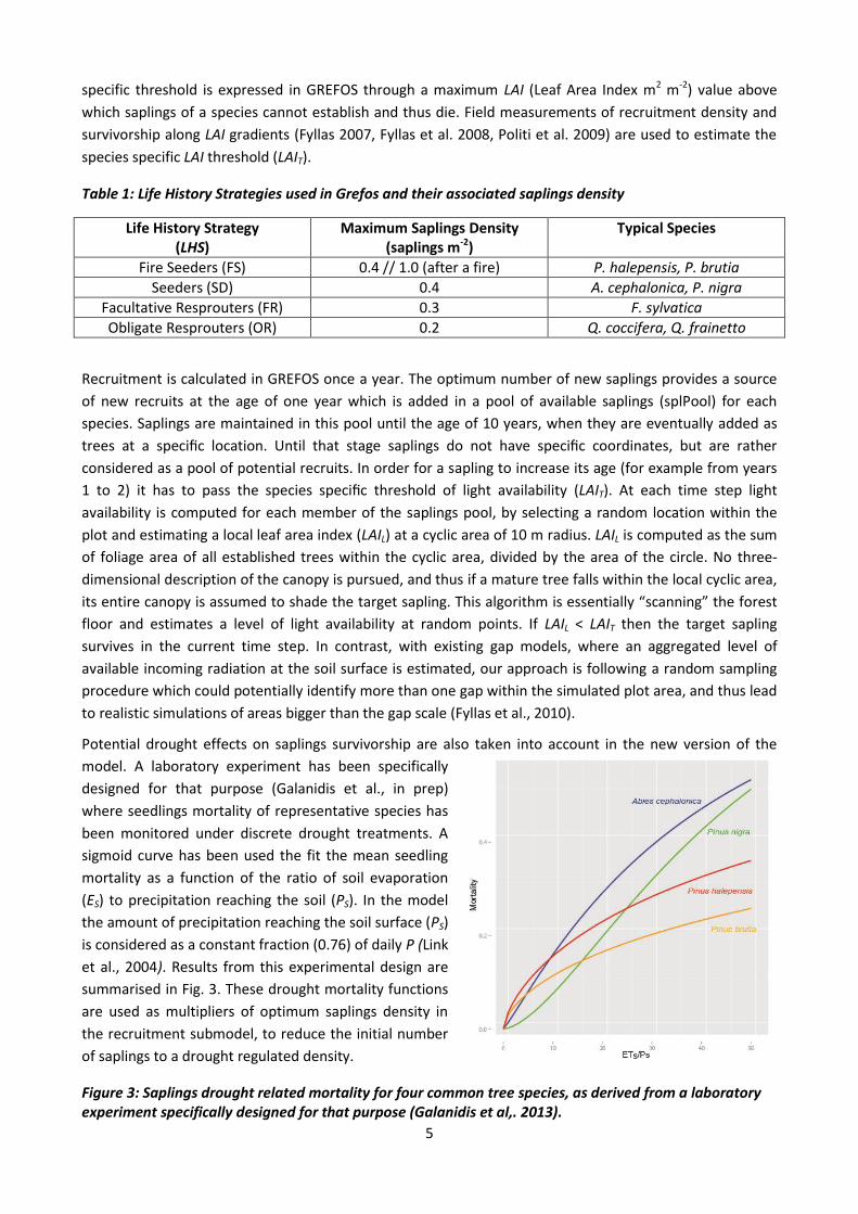
Potential drought effects on saplings survivorship are also taken into account in the new version of the

model. A laboratory experiment has been specifically

designed for that purpose (Galanidis et al., in prep)

where seedlings mortality of representative species has

been monitored under discrete drought treatments. A

sigmoid curve has been used the fit the mean seedling

mortality as a function of the ratio of soil evaporation

(ES) to precipitation reaching the soil (PS). In the model

the amount of precipitation reaching the soil surface (PS)

is considered as a constant fraction (0.76) of daily P (Link

et al., 2004). Results from this experimental design are

summarised in Fig. 3. These drought mortality functions

are used as multipliers of optimum saplings density in

the recruitment submodel, to reduce the initial number

of saplings to a drought regulated density.

Figure 3: Saplings drought related mortality for four common tree species, as derived from a laboratory experiment specifically designed for that purpose (Galanidis et al,. 2013).

6

Light Competition

Competition for light is the basic competitive process simulated in GREFOS. Two alternative formulations

are implemented in the current version of the model.

The first method is the standard light competition algorithm used in forest gap dynamic models, where a

competitive hierarchy based on height is assumed (Shugart 1984). Following this algorithm taller trees are

assumed to shade all smaller trees and a cumulative shading LAI (SLAI) is estimated for each tree in the

stand as:

1

1 j m

i j

j

SLAI FAA

(17), for each tree i with j=1...m all trees with Hj>Hi

The second method follows the Perfect Plasticity model of Purves et al. (2007). Following this formulation

trees are characterised as canopy or subcanopy (in or out of canopy). The flat-top version ignores crown

depth and assumes that all of a tree’s foliage is found at the top of its stem. A canopy height Z* is estimated

for a forest stand defining canopy and subcanopy trees. By summing up the crown area (CA) of all trees in

the stand, Z* is defined as the height of the last tree that enters to the sum before the cumulative crown

area is equal to the plot area.

Results from the first light competition formulation are only presented here.

Growth Submodel

In most forest gap dynamics models the idea of optimum growth curve is used to estimate the annual

diameter increment. This algorithm is assuming that for a given size an individual tree of a certain species

can achieve an optimum growth, which is then modified by a number of abiotic and biotic factors that

represent the non optimum growth conditions in terms of climate and/or competition. In this version of

the model, an optimum growth curve has been estimated from annual tree ring width data which are site

and species specific. Three environmental factors that reduce optimum growth have been selected, i.e.

light availability, heat time (or growing degree days) and water availability.

The optimum growth of an individual (gO in mm) is described by the equation proposed by Zeide (1993),

(see also Fyllas et al., 2012):

2

log

exp 0.5O

O m

b

D

Dg G

D

(18)

where Gm is the maximum potential growth rate (mm y-1) at the peak of the log-normal growth curve, D0 is

the diameter at breast height (D) associated with the maximum growth rate, and Db determines the

breadth of the curve. Tree rings data for a minimum of ten individual trees per species are used to estimate

the parameters of equation 18, with a summary of some common tree species given in Table 2. The shape

of the optimum growth curve is illustrated in Fig. 4.

Table 2: Optimum growth parameters for some common species in Greece

7

Species Gm (mm y-1) DO (cm) Db (-)

Abies cephalonica 11.3 9.12 1.54

Pinus halepensis 17.2 8.90 -1.50

Pinus brutia 19.2 7.09 1.22

Pinus nigra 15.0 6.75 1.61

Quercus ilex 6.0 1.11 1.69

Quercus frainetto 10.7 1.12 2.06

Figure 4: Optimum growth curves for some common tree species

For each tree in the plot an actual growth rate (ga cm y-1) is subsequently calculated by:

13( )a Og g LRF TRF DRF (19)

where LRF, TRF and DRF the light,

temperature and drought response function

respectively.

The light response function is given from:

1 2 31 exp ( )iLRF a a I a (20)

where Ii is the relative to top canopy

available light for tree i, and α1, α2 and α3

species specific parameters as in Mailly et al.

(2000), which define five shade tolerance

classes (Fig. 5).

Figure 5: Light response function for the five shade tolerance classes

The temperature response function used in GREFOS v1 (Fyllas et al., 2007) and parameterised for the

dominant woody taxa in Greece is also used here:

8

min1 expTRF q GDD GDD (21)

Where q is a constant coefficient (q=0.0013) and GDDmin a species specific threshold of minimum heat time

requirements. GDD is defined as the annual sum of growing degree days with a temperature base of 5 oC.

The original drought response function has been re-parameterised in the current version of the model.

Based on the soil water balance algorithm (equations 10 & 13), drought days are defined as those days

where Θ<0.1. A daily drought index (DI) is then estimated as DIi=1-Θi, while over the course of a year the

annual DI is calculated from the sum of daily DIi. The response function of six drought tolerance classes is

given from:

1DRF DI (22)

where δ a tolerance class specific coefficient ranging from 0.012 for class 1, 0.0084 for class 2, 0.0073 for

class 3, 0.0063 for class 4, 0.0055 for class 5 and 0.0047 for class 6.

Mortality Submodel

Three sources of mortality are considered in GREFOS (Fyllas et al. 2007). The intrinsic or maximum age-

dependent mortality (Πim) assumes that only 2% of a species population reaches its maximum age (Keane et

al., 2001) and it is estimated annually for each tree in the stand from:

max

4.6051 exp( )im

Age

(23), where Agemax the species specific maximum age.

The growth-dependent mortality (Πgm) applies to trees that are not able to achieve an adequate growth for

two consecutive years (Solomon 1986, Bigler & Bugmann 2004). These trees are assumed to have a lower

survival probability with Πgm = 0.632. The threshold for adequate growth is set here as the 10% of the

optimum radial growth that a tree of a certain species and size would achieve, i.e ga<0.1go.

The disturbance-dependent mortality (Πdm) is linked with the LHS of a tree and takes place only when the

stand burns. Species belonging to the seeder (SD) and fire seeder (FS) group are assumed to completely

burn and thus Πdm=1 after a fire event. Facultative resprouters (FR) have a small probability of resprouting

and thus for individuals of this group Πdm=0.8 after a fire. Obligative resprouters (OR) have a higher survival

probability and thus in this case Πdm=0.3.

Fire Submodel

A fire probability is estimated on a daily basis based on the prevailing weather conditions, the structure of

the stand and the moisture content of the fuel. The moisture content of the fuel (FMC) is estimated from

the empirical equation given in Sharples et al. (2009):

10 0.25 ( )FMC T RH (24) where T the daily mean temperature (oC) and RH the relative humidity

of the air (%).

Fuel moisture of extinction (ME), i.e. the fuel moisture content above which a fire cannot be sustained, is

estimated based on the relative contribution of each species to the overall fuel bed, with each species

9

characterised by a specific ME (Dimitrakopoulos & Papaioannou 2001, Fyllas et al. 2009). The daily ignition

probability is then given (Chuvieco et al. 2004):

ign

max

ign

min

FMC>ME: Π 0.2 1

: Π 0.2 0.8

FMC MEif

FMC ME

ME FMCelse

ME FMC

(25)

with FMCmax and FMCmin the maximum and minimum FMC values reported in Aguado et al. (2007).

The daily probability of having a crown fire is the estimated assuming that one third of ignitions become

crown fires as:

1

3Fire ign (26)

Figure 6: Daily average temperature (T), fuel moisture content (FMC) and fire probability (ΠFire) over the course of a year on Mt Taygetos (1300m asl).

Simulation Exercises

In the following section we provide a set of simulation exercises at three study areas in Greece with

contrasting climate patterns. In all study areas the vegetation is dominated by coniferous forest. The

dominant species are: Pinus halepensis, Pinus brutia, Pinus nigra and Abies cephalonica. Field observations

and laboratory experiments are available for the study sites and species of interest. The aim of these

simulations is to verify the ability of GREFOS to reconstruct the vegetation patterns and fire regime across

the study sites.

10

Taygetos P.nigra /A.cephalonica study site:

Mount Taygetos is found at the southern part of continental Greece. Along a heterogenous landscape with

an altitude reaching up to 2400 m asl different forest types are established, but the dominant forest tree

species above 600m asl are P. nigra and A. cephalonica. In general P. nigra is more drought tolerant

compared to A. cephalonica and it is usually found at swallower soils. The ability of the model to shift the

vegetation type with changing soil depths was the purpose of the simulation exercise at Mt. Taygetos. Thus

at an altitude of 1000 m asl the model was set to run for 750 from bare ground, using again the first 250

years as a "spin-up" period. An additional test of model realism was to compare the simulated MFI with

fire-scars data available for the black pine forest in this area (Christopoulou et al. 2013). At swallow soils of

0.1m depth P. nigra dominates the stand. With increasing soil depth A. cephalonica increases its

contribution to the stand biomass, with a complete dominance above soil depths of 0.3m. The MFI ranged

from 32 to 34 and to 39 years respectively for increasing soil depth. These estimates were similar to an

MFI=30 years measured for this area (Christopoulou et al. 2013).

11

Parnitha P. halepensis /A.cephalonica study site:

At this study area the model was used to explore for potential effects of climatic changes on the dynamics

of vegetation. Forest stands at an altitude of 1300m asl , with a soil depth of 0.5m were selected, where

currently the endemic Greek fir species (A. cephalonica) is the dominant element of vegetation. A

comparison between simulations forced with the current climate and a B2 (increase of 2oC in annual

temperature and decrease of 5% in precipitation) climate change scenario would highlight potential effects

of shifting climate patterns. Under current climatic condition fir dominates the stands with a mean fire

return interval of 120 years. However under an increase in temperature and slight decrease in precipitation

the model simulates a change in the species synthesis of these stands with a significant increase of P.

halepensis and a decrease of MFI to 64 years.

Lesbos P. brutia / P. nigra study site:

At this study site a mixed P. brutia / P nigra forest is established at elevations above 600 m asl with

unburned northern areas dominated by P. nigra (Fyllas et al. 2008). P. brutia is a drought tolerant pine

adapted to persist to frequent fires through a fire seeding strategy and dominates at low elevation. P nigra

is a less drought tolerant pine which forms extensive forest throughout Europe and Greece at the sub-

Mediterranean zone. The model was set up to run at an altitude of 700m asl, with a soil depth of 0.5 and a

medium soil water holding capacity profile for 750 years. The first 250 years are used a model "spin-up"

phase Two simulations experiments were designed ("fire on" and "fire off") to test whether climate or fire

is the dominant agent forming the established vegetation patterns. In the first case the model estimated a

mean fire return interval (MFI) of 77 years, by fitting a Weibull distribution to the intervals between

successive fires (Johnson 1994, Fyllas and Troumbis 2009). In the second case the fire algorithm was

turned-off (i.e. MFI=∞) and thus the only source of disturbance driving forest dynamics was gap

development. A summary of vegetation development, from bare ground, indicates that the dominance of

P. brutia and the mixed profile of vegetation at higher altitudes is driven by the local fire regime. Given the

local climate profile, exclusion of fire lead to P. nigra dominated stands. These simulations are in

agreement with field observations from the study site (Fyllas et al. 2008).

12

References

Aguado, I., Chuvieco, E., Boren, R., Nieto, H., 2007. Estimation of dead fuel moisture content from

meteorological data in Mediterranean areas. Applications in fire danger assessment. International

Journal of Wildland Fire 16, 390–397.

Bigler, C., Bugmann, H., 2004. Predicting the time of tree death using dendrochronological data. Ecological

Applications 14, 902–914.

Botkin, D.B., Janak, J.F., Wallis, J.R., 1972. Some ecological consequences of a computer model of forest

growth. The Journal of Ecology 849–872.

Bugmann, H., Cramer, W., 1998. Improving the behaviour of forest gap models along drought gradients.

Forest Ecology and Management 103, 247–263.

Chuvieco, E., Aguado, I., Dimitrakopoulos, A.P., 2004. Conversion of fuel moisture content values to ignition

potential for integrated fire danger assessment. Canadian Journal of Forest Research 34, 2284–2293.

Dimitrakopoulos, A.P., 2002. Mediterranean fuel models and potential fire behaviour in Greece.

International Journal of Wildland Fire 11, 127–130.

Flint, A.L., Childs, S.W., 1991. Use of the Priestley-Taylor evaporation equation for soil water limited

conditions in a small forest clearcut. Agricultural and Forest Meteorology 56, 247–260.

Fyllas, N.M., Dimitrakopoulos, P.G., Troumbis, A.Y., 2008. Regeneration dynamics of a mixed Mediterranean

pine forest in the absence of fire. Forest Ecology and Management 256, 1552–1559.

Fyllas, N.M., Phillips, O.L., Kunin, W.E., Matsinos, Y.G., Troumbis, A.I., 2007. Development and

parameterization of a general forest gap dynamics simulator for the North-eastern Mediterranean

Basin (GREek FOrest Species). ecological modelling 204, 439–456.

Fyllas, N.M., Politi, P.I., Galanidis, A., Dimitrakopoulos, P.G., Arianoutsou, M., 2010. Simulating regeneration

and vegetation dynamics in Mediterranean coniferous forests. Ecological Modelling 221, 1494–1504.

13

Fyllas, N.M., Troumbis, A.Y., 2009. Simulating vegetation shifts in north-eastern Mediterranean mountain

forests under climatic change scenarios. Global Ecology and Biogeography 18, 64–77.

Gracia, C.A., Tello, E., Sabaté, S., Bellot, J., 1999. GOTILWA: An integrated model of water dynamics and

forest growth, in: Ecology of Mediterranean Evergreen Oak Forests. Springer, pp. 163–179.

Hsiao, T.C., Heng, L., Steduto, P., Rojas-Lara, B., Raes, D., Fereres, E., 2009. AquaCrop—The FAO crop model

to simulate yield response to water: III. Parameterization and testing for maize. Agronomy Journal

101, 448–459.

Kazanis, D., Arianoutsou, M., 1996. Vegetation composition in a post-fire successional gradient of Pinus

halepensis forests in Attica, Greece. International Journal of Wildland Fire 6, 83–91.

Mailly, D., Kimmins, J.P., Busing, R.T., 2000. Disturbance and succession in a coniferous forest of

northwestern North America: simulations with DRYADES, a spatial gap model. Ecological modelling

127, 183–205.

Pausas, J.G., 1999. Response of plant functional types to changes in the fire regime in Mediterranean

ecosystems: a simulation approach. Journal of Vegetation Science 10, 717–722.

Pausas, J.G., Bradstock, R.A., Keith, D.A., Keeley, J.E., 2004. Plant functional traits in relation to fire in

crown-fire ecosystems. Ecology 85, 1085–1100.

Politi, P.I., Arianoutsou, M., Stamou, G.P., 2009. Patterns of< i> Abies cephalonica</i> seedling recruitment

in Mount Aenos National Park, Cephalonia, Greece. Forest Ecology and Management 258, 1129–

1136.

Purves, D.W., Lichstein, J.W., Pacala, S.W., 2007. Crown plasticity and competition for canopy space: a new

spatially implicit model parameterized for 250 North American tree species. PLoS One 2, e870.

Risch, A.C., Heiri, C., Bugmann, H., 2005. Simulating structural forest patterns with a forest gap model: a

model evaluation. Ecological Modelling 181, 161–172.

Sharples, J.J., McRae, R.H.D., Weber, R.O., Gill, A.M., 2009. A simple index for assessing fire danger rating.

Environmental Modelling & Software 24, 764–774.

Shugart, H.H., 1984. A theory of forest dynamics. The ecological implications of forest succession models.

Springer-Verlag.

Solomon, A.M., 1986. Transient response of forests to CO2-induced climate change: simulation modeling

experiments in eastern North America. Oecologia 68, 567–579.

Steduto, P., Hsiao, T.C., Raes, D., Fereres, E., 2009. AquaCrop—The FAO crop model to simulate yield

response to water: I. Concepts and underlying principles. Agronomy Journal 101, 426–437.

Wösten, J.H.M., Lilly, A., Nemes, A., Le Bas, C., 1999. Development and use of a database of hydraulic

properties of European soils. Geoderma 90, 169–185.

Wösten, J.H.M., Pachepsky, Y.A., Rawls, W.J., 2001. Pedotransfer functions: bridging the gap between

available basic soil data and missing soil hydraulic characteristics. Journal of Hydrology 251, 123–150.

Zeide, B., 1993. Analysis of growth equations. Forest science 39, 594–616.