Martingale theory lecture notes

Marton Balazs∗∗

October 29, 2018

These notes summarise the lectures and exercise classes Martingale Theory with Applications of Autumn2018 in the University of Bristol.

Contents

1 A quick summary of some parts of measure theory 2

2 Conditional expectation and a toy example 5

3 Probability toolbox 7

4 Modes of convergence 9

5 Uniform integrability 10

6 Martingales, stopping times 12

7 Martingale convergence 16

8 Uniformly integrable martingales 18

9 Doob’s submartingale inequality 20

10 A discrete Black-Scholes option pricing formula 21

∗School of Mathematics, University of Bristol

1

1 A quick summary of some parts of measure theory

. . . from the probabilist point of view. This section mostly follows Shiryaev [1]. The aim is to build up amathematical model of random experiments and measurements (random variables, that is) thereof. Probabilitiesof these random outcomes are also to be constructed. As this is a short summary for a short unit, we leaveseveral proofs for another unit Further Topics in Probability (FTiP).

The power set P(Ω) of a set Ω is the set of all subsets of Ω, and Ac : = Ω−A denotes the complement of aset A ⊆ Ω.

Definition 1.1. A family A ⊆ P(Ω) of sets is called an algebra, if

• Ω ∈ A,

• for every A, B ∈ A, A ∪B ∈ A,

• for every A ∈ A, Ac ∈ A.

This simple construction allows us to build a prototype of probabilities as follows.

Definition 1.2. Let A be an algebra. A set function µ : A → [0, ∞] is a finitely additive measure on A, if forall disjoint A, B ∈ A,

µ(A ∪B) = µ(A) + µ(B).

As it turns out, the objects we defined so far are too general for our purposes, hence a refinement comesnext.

Definition 1.3. A family F ⊆ P(Ω) of sets is called a σ-algebra, if

• Ω ∈ F ,

• for every countably many sets A1, A2, · · · ∈ F ,⋃

n An ∈ F ,

• for every A ∈ F , Ac ∈ F .

In this case the pair (Ω, F) is called a measurable space. Any set A ∈ F is said to be F-measurable, or justmeasurable.

The novelty here is the requirement of F being closed for countably infinite unions, as opposed to finite unionsonly for an algebra.

Example 1.4. Here are examples of σ-algebras (check!).

• F∗ = ∅, Ω is called the trivial σ-algebra.

• If Ω is countable, very often F∗ = P(Ω) is considered, which is a σ-algebra in this case.

• For a set A ⊂ Ω, FA = ∅, A, Ac, Ω is the σ-algebra generated by A.

Definition 1.5. A measure µ on an algebra A is a set function µ : A → [0, ∞] such that for any mutuallydisjoint sets A1, A2, · · · ∈ A with

⋃

n An ∈ A,

(1.1) µ(

∞⋃

n=1

An

)

=

∞∑

n=1

µ(An)

holds. If µ(Ω) = 1, then we call µ a probability measure, and often use P instead. In this case the triplet(Ω, F , P) is called a probability space.

Notice that a σ-algebra is automatically an algebra, thus this definition applies for measures on σ-algebras.Property (1.1) is referred to as σ-additivity.

When modeling a random experiment, the set Ω is called the sample space of the experiment, it contains allelementary outcomes. Its measurable subsets A ∈ F are called events. These are exactly those sets of outcomeswhich have a probability. The empty set ∅ is always an event, called the null event. The above definitions implythat P(∅) = 0.

Here is a rather useful characterisation of probability measures.

Theorem 1.6. Let P be a finitely additive measure on an algebra A, and assume P(Ω) = 1. Then the followingare equivalent.

1. P is a probability measure.

2

2. If (An)n≥1 is an increasing sequence of sets in A (that is, An ⊆ An+1 for n ≥ 1) and⋃∞

n=1 An ∈ A, thenthe below limit exists, and

limn→∞

P(An) = P

(

∞⋃

n=1

An

)

.

3. If (An)n≥1 is a decreasing sequence of sets in A (that is, An ⊇ An+1 for n ≥ 1) and⋂∞

n=1 An ∈ A, thenthe below limit exists, and

limn→∞

P(An) = P

(

∞⋂

n=1

An

)

.

4. If (An)n≥1 is a decreasing sequence of sets in A and⋂∞

n=1 An = ∅, then the below limit exists, and

limn→∞

P(An) = 0.

Notice that the union of increasing sets, and the intersection of decreasing sets, are sometimes called the limitof the sets. We leave the proof of this theorem to FTiP.

We now proceed with a short summary on how some commonly used σ-algebras are constructed. Here isthe main tool for this:

Lemma 1.7. Let E ⊆ P(Ω). Then

• there is a smallest algebra α(E) that contains all sets from E;

• there is a smallest σ-algebra σ(E) that contains all sets from E.

Proof. The intersection of algebras is an algebra, and the intersection of σ-algebras is a σ-algebra. To find theones in the lemma, take the intersection of all algebras, respectively σ-algebras, that contain all sets in E .

The above α(E) and σ(E) are said to be generated by E .Let us now consider

(1.2) A : =

n⋃

i=1

(ai, bi] : n < ∞, and a1 < b1 ≤ a2 < b2 ≤ . . . in R ∪ −∞, ∞

.

This is an algebra (check!), but not a σ-algebra: each of(

0, 1− 1n

]

is in A, but the union of these sets for all nis (0, 1), which is not in A. However, this algebra can be used to generate the following σ-algebra:

Definition 1.8. The Borel σ-algebra on R, denoted B(R), is the σ-algebra generated by (1.2). Sets in B(R)are said to be Borel sets.

This σ-algebra contains all subsets of R that are ”of practical interest”. I.e., it is not easy to come up witha non-Borel set in R. Those interested can look up the Vitali set for an example.

In a similar way, n-dimensional rectangles:

(a1, b1]× (a2, b2]× · · · × (an, bn] : a1 < b1, a2 < b2, . . . , an < bn in R

,

rather than one-dimensional intervals, can be used to generate B(Rn), the Borel σ-algebra on Rn. This willcontain ”all n-dimensional sets of practical interest”.

One can then proceed to R∞, the set of real-valued sequences, by considering the σ-algebra B(R∞) generatedby rectangles of arbitrary finite dimension. Again, ”practical sets”, such as

(xn) : limn→∞

xn exists and is finite

;

(xn) : supn

xn > 5

;

(xn) : lim infn→∞

xn > 5

all belong to B(R∞).One can even define B(RT ) with an uncountable set T , for example σ-algebras on function spaces. This

usually requires some restrictions on the family of functions considered.The next theorem, which we cover without proof, allows to construct measures on generated σ-algebras.

Theorem 1.9 (Caratheodory). Let A be an algebra on Ω. If µ0 is a σ-additive measure on (Ω, A), then thereexists a unique extension of it to

(

Ω, σ(A))

(the generated σ-algebra).

Definition 1.10. Let F : R → [0, 1] be a cumulative distribution function, and define the σ-additive measureP on (1.2) by P(a, b] : = F (b)− F (a). This extends to the Lebesgue-Stieltjes measure on

(

R, B(R))

.

3

When F is the Uniform(0, 1) distribution, we obtain the Lebesgue measure on B([0, 1]) this way.We briefly mention that P can be extended to Rn in a natural way, then Kolmogorov’s extension theorem

can be used, under certain circumstances, to extend further to R∞ or even RT .The next task is to construct random variables on a probability space (Ω, F , P).

Definition 1.11. Let (Ω, F) be a measurable space. A function X : Ω → R is called measurable, if for anyB ∈ B(R), X−1(B) ∈ F . A (real-valued) random variable on a probability space (Ω, F , P) is a measurablefunction from X : Ω → R.

It should now be clear how probabilities associated with random variables work. The above definition exactlysays that a random variable taking values in a Borel set B ∈ B(R) is an event in our probability space (i.e.,belongs to F). As an example, let us consider the distribution function F of a random variable. When firstencountered, it is usually defined as F (x) = PX ≤ x. With the above construction, it should rather bewritten as

F (x) = Pω ∈ Ω : X(ω) ≤ x = P

X−1(−∞, x]

.

which of course has the same meaning, we just understand properly now what is behind the notation. The set(−∞, x] ∈ B(R) is a Borel set, X is a measurable function which implies that X−1(−∞, x] ∈ F , hence this isan event and it makes sense to talk about its probability in the sample space Ω.

We remark that limits, sums, differences, products, ratios (where defined), Borel-measurable functions ofrandom variables are each random variables again, in other words these operations do not ruin measurability.

Next we briefly summarise without proofs how to construct expectations of random variables. (In measuretheory, this would be called integrals of measurable functions.) We sometimes omit mentioning the probabilityspace (Ω, F , P).

Definition 1.12. A random variable X is called simple, if there exist n > 0, x1, x2, . . . , xn ∈ R, andA1, A2, . . . , An ∈ F with which

X(ω) =

n∑

k=1

xk · 1Ak(ω).

Here 1A stands for the indicator function:

1A(ω) =

1, if ω ∈ A,

0, if ω /∈ A.

Theorem 1.13.

(a) For any random variable X there exists a sequence X1, X2, . . . of simple random variables such that|Xn| ≤ |X | for all n, and Xn(ω) → X(ω) as n → ∞ for all ω ∈ Ω.

(b) Moreover, if X(ω) ≥ 0 for every ω ∈ Ω, then Xn can be chosen to be non-decreasing in n for every fixedω ∈ Ω (denoted Xn(ω) ր X(ω) as n → ∞ for all ω ∈ Ω).

Definition 1.14 (Expectations).

(a) If X is simple with X =∑n

k=1 xk · 1Ak, then EX : =

∑nk=1 xk · P(Ak).

(b) If X ≥ 0 is a random variable, then EX : = limn→∞ EXn, where Xn ր X are simple random variables.(Such sequence exists by the above, and it is a theorem that this limit does not depend on the choice ofthe sequence.) Notice that EX = ∞ is possible.

(c) If X is a random variable, EX : = EX+ − EX−, unless both expectations on the right-hand side areinfinite, in which case EX is not defined.

Here the positive and negative parts are used:

(1.3) x+ = x · 1x > 0, x− = −x · 1x < 0, x = x+ − x− for any x ∈ R.

Notice that options for EX are ”not defined”, = ∞, = −∞, or ∈ R.

4

2 Conditional expectation and a toy example

We start this section with Kolmogorov’s Theorem on conditional expectations from Williams [2]. Notation:E(· ; G) : = E(·1G).

Theorem 2.1. Let X be a random variable on the probability space (Ω, F , P), with E|X | < ∞. Let G be a subσ-algebra. Then there exists a random variable V such that

(a) V is G-measurable,

(b) E|V | < ∞,

(c) E(V ; G) = E(X ; G) for any G ∈ G.

This V is unique up to zero-measure sets and is called a version of the conditional expectation E(X | G).Our toy example will be the following. Let Ω = 1, 2, . . . , 12, F = P(Ω), and P be the uniform measure

on the finite set Ω. Elementary outcomes in Ω will be denoted by ω. Define the random variables

Y : =⌈ω

4

⌉

=

1, if ω = 1, 2, 3, 4,

2, if ω = 5, 6, 7, 8,

3, if ω = 9, 10, 11, 12,

X : =⌈ω

2

⌉

=

1, if ω = 1, 2,

2, if ω = 3, 4,

3, if ω = 5, 6,

4, if ω = 7, 8,

5, if ω = 9, 10,

6, if ω = 11, 12.

The σ-algebra generated by Y is

G : = σ(Y ) : = σ(

Y −1(

B(R)))

= σ(

1, 2, 3, 4, 5, 6, 7, 8, 9, 10, 11, 12)

=

∅, 1, 2, 3, 4, 5, 6, 7, 8, 9, 10, 11, 12,1, 2, 3, 4, 5, 6, 7, 8, 1, 2, 3, 4, 9, 10, 11, 12, 5, 6, 7, 8, 9, 10, 11, 12, Ω

.

Similarly, the σ-algebra generated by X is

H : = σ(X) : = σ(

X−1(

B(R)))

= σ(

1, 2, 3, 4, 5, 6, 7, 8, 9, 10, 11, 12)

.

We see that G ⊂ H ⊂ F . The σ-algebra G is coarser (contains less information), while H is finer (moreinformation). We also see that

• Y is G-measurable (by definition).

• Y is H-measurable (due to G ⊂ H).

• X is H-measurable (by definition).

• X is not G-measurable (e.g., X−11 = 1, 2 /∈ G).

Next, we find the conditional expectation E(X | G) based on the definition above. As G = σ(Y ), an equivalentnotation for this is E(X | G) = E(X |Y ). Due to |Ω| = 12 < ∞, finite mean of V = E(X | G) is not an issue. Welook for a G-measurable random variable V with E(V ; G) = E(X ; G) for any G ∈ G. An efficient choice for Gis 1, 2, 3, 4. As V is G-measurable, and G has no set that distinguishes between these four outcomes, we findthat V (ω) is the same for ω = 1, 2, 3, 4. The above expectations turn into

V (1)P1+ V (2)P2+ V (3)P3+ V (4)P4 = X(1)P1+X(2)P2+X(3)P3+X(4)P4V (1)P1+ V (1)P2+ V (1)P3+ V (1)P4 = X(1)P1+X(2)P2+X(3)P3+X(4)P4

V (1) = V (2) = V (3) = V (4) =1 · 1

12 + 1 · 112 + 2 · 1

12 + 2 · 112

112 + 1

12 + 112 + 1

12

= 1.5.

Similarly, with the respective choices G = 5, 6, 7, 8 and G = 9, 10, 11, 12,

V (5) = V (6) = V (7) = V (8) =3 · 1

12 + 3 · 112 + 4 · 1

12 + 4 · 112

112 + 1

12 + 112 + 1

12

= 3.5,

V (9) = V (10) = V (11) = V (12) =5 · 1

12 + 5 · 112 + 6 · 1

12 + 6 · 112

112 + 1

12 + 112 + 1

12

= 5.5.

5

Hence the conditional expectation is the random variable

E(X | G)(ω) = V (ω) =

1.5, if ω = 1, 2, 3, 4,

3.5, if ω = 5, 6, 7, 8,

5.5, if ω = 9, 10, 11, 12,

being just the average of X over the smallest nontrivial respective units in G.In a similar way one can check

E(Y | G)(ω) =

1, if ω = 1, 2, 3, 4,

2, if ω = 5, 6, 7, 8,

3, if ω = 9, 10, 11, 12

= Y (ω),

and indeed it is always the case that E(Y |Y ) = Y almost everywhere (a.e.).Further examples are E

(

X | ∅, Ω)

, where the random variable V we are looking for is measurable w.r.t.the trivial σ-algebra ∅, Ω, in other words is a constant. Picking G = ∅ gives E(V ; ∅) = 0 = E(X ; ∅), whichis not very informative. The choice G = Ω on the other hand fixes the value of the constant V :

E(V ; Ω) = E(X ; Ω)

EV = EX

V = EX,

that is, E(

X | ∅, Ω)

= EX . This is again true a.e. in general, conditioning on the trivial σ-algebra alwaysproduces a full expectation.

If, on the other hand, one conditions on the full σ-algebra F that has all information that can be availablein the probability space (Ω, F , P), then every event G ∈ F can be substituted, and the very detailed onescompletely fix the conditional expectation. In our example we can e.g., take 7 to obtain

E(V ; 7) = E(X ; 7),V (7) · P7 = X(7) · P7,

V (7) = X(7) = 4.

Similarly, for any ω ∈ Ω one has V (ω) = X(ω), which leads us to E(X | F) = V = X . This is again a.e. true forgeneral probability spaces: conditioning on the full information does not do any averaging and gives back therandom variable instead.

Our final example is

I : = σ(

1, 5, 9, 3, 7, 11)

=

∅, 1, 5, 9, 3, 7, 11, 2, 4, 6, 8, 10, 12, 1, 3, 5, 7, 9, 11,1, 2, 4, 5, 6, 8, 9, 10, 12, 2, 3, 4, 6, 7, 8, 10, 11, 12, Ω

.

We compute V = E(Y | I) as before. This is I-measurable, hence constant on 1, 5, 9, as well as on 3, 7, 11and on 2, 4, 6, 8, 10, 12. Substituting these as G (the rest in I will not provide additional help) in E(V ; G) =E(Y ; G) results in

V (1) = V (5) = V (9) =Y (1)P1+ Y (5)P5+ Y (9)P9

P1+ P5+ P9 =1 · 1

12 + 2 · 112 + 3 · 1

12112 + 1

12 + 112

= 2,

V (3) = V (7) = V (11) =Y (3)P3+ Y (7)P7+ Y (11)P11

P3+ P7+ P11 =1 · 1

12 + 2 · 112 + 3 · 1

12112 + 1

12 + 112

= 2,

V (2) = V (4) = V (6)

= V (8) = V (10) = V (12) = Y (2)P2+Y (4)P4+Y (6)P6+Y (8)P8+Y (10)P10+Y (12)P12P2+P4+P6+P8+P10+P12

=1 · 1

12 + 1 · 112 + 2 · 1

12 + 2 · 112 + 3 · 1

12 + 3 · 112

112 + 1

12 + 112 + 1

12 + 112 + 1

12

= 2.

We find that E(Y | I) is actually a constant, and in fact = EY .We can repeat this calculation with any function f : R → R (in general this is chosen to be bounded and

measurable) to find E(

f(Y ) | I)

= E(

f(Y ))

, a constant. This is when we say that the random variable Y isindependent of the σ-algebra I. Knowing which of the events 1, 5, 9 and 3, 7, 11 did or did not happenwill not tell us any information about Y .

If I happens to be generated by yet another random variable Z, I = σ(Z), then the above is equivalent tovariables Y and Z being independent.

An important property and tool with conditional expectations is the following:

6

Theorem 2.2 (Tower rule). Let Z be a random variable on the probability space (Ω, F , P), with E|Z| < ∞.Let G ⊆ H be sub σ-algebras (G is coarser and H is finer). Then

E(

E(Z | G) | H)

= E(

E(Z | H) | G)

= E(Z | G).

The proof follows from the definition of conditional expectations after a bit of manipulations, we leave this tothe reader. Some special cases of interest:

• If H = F , the full σ-algebra in the probability space (Ω, F , P), then E(Z | H) = E(Z | F) = Z for anyrandom variable. The above then reads E(Z | G) for all three terms.

• If G = ∅, Ω, the trivial σ-algerba, then E(· | G) = E(·). The Tower rule then becomes

E(

(EZ) | H)

= E(

E(Z | H))

= EZ.

The first of these terms is uninteresting, but the second equality is very useful and might be familiar fromearlier studies, especially when H = σ(V ), the σ-algebra generated by another random variable V . In thiscase it reads E

(

E(Z|V ))

= EZ.

3 Probability toolbox

The following statements are widely used across probability, and will be built on in this unit. Several proofsare omitted, most of those can be found in the unit FTiP. We always assume the probability space (Ω, F , P)in the background.

We start with an important fact from calculus.

Lemma 3.1. Let ak ∈ (0, 1) with limk→∞ ak = 0. Then

∞∏

k=1

(1 − ak) = 0 ⇔∑

k

ak = ∞.

Proof. Convexity of the exponential function implies 1 − x ≤ e−x for any x ∈ R. As terms in the product arenon-negative,

∞∏

k=1

(1− ak) ≤∞∏

k=1

e−ak = e−∑

∞

k=1ak .

This proves ⇐.The function e−2x is smooth with value 1 and derivative −2 at x = 0. Hence for all small enough x > 0,

1− x ≥ e−2x. There is an index K that makes ak small enough for this purpose for any k ≥ K. Therefore

∞∏

k=K

(1− ak) ≥∞∏

k=K

e−2ak = e−2∑

∞

k=K ak .

If∏∞

k=1(1− ak) = 0, then the left hand-side above is also zero, which proves ⇒.

Definition 3.2. Let A1, A2, . . . be events. Then

lim supn

An : =∞⋂

n=1

∞⋃

k=n

Ak.

By decoding the union and the intersection it becomes clear that this event describes that infinitely many ofthe An’s occur, in other words An’s occur infinitely often (i.o.).

Theorem 3.3 (Borel-Cantelli lemmas).

1. If A1, A2, . . . are any events with∑

n P(An) < ∞, then P(lim supn An) = 0.

2. If A1, A2, . . . are independent events with∑

n P(An) = ∞, then P(lim supn An) = 1.

Proof.

1. Notice that⋃∞

k=n Ak is decreasing in n. Thus, by continuity of probability (Theorem 1.6) and Boole’sinequality,

P

(

∞⋂

n=1

∞⋃

k=n

Ak

)

= limn→∞

P

(

∞⋃

k=n

Ak

)

≤ limn→∞

∞∑

k=n

P(Ak) = 0.

7

2. Notice that⋂∞

k=n Ack is increasing in n. Thus,

P

(

∞⋂

n=1

∞⋃

k=n

Ak

)

= 1− P

(

∞⋃

n=1

∞⋂

k=n

Ack

)

= 1− limn→∞

P

(

∞⋂

k=n

Ack

)

= 1− limn→∞

∞∏

k=n

(

1− P(An))

.

The product is 0 for any n due to Lemma 3.1, which completes the proof.

We now turn to interchangeability of limits and expectations. The below are standard parts of measuretheory, where they are treated for more general integrals than just expectations and sums as here.

The proofs of the following theorems are skipped (can be found in FTiP).

Theorem 3.4 (Monotone convergence). Let Y, X, X1, X2, X3, . . . be random variables.

• If Xn ≥ Y for each n, EY > −∞, and Xn ր X for every ω ∈ Ω, then EXn ր EX.

• If Xn ≤ Y for each n, EY < ∞, and Xn ց X for every ω ∈ Ω, then EXn ց EX.

For the next statement, notice that every sequence has a liminf.

Theorem 3.5 (Fatou’s lemma). Let Y, X1, X2, X3, . . . be random variables with Xn ≥ Y for each n, EY >−∞. Then lim infn EXn ≥ E lim infn Xn.

It is sometimes convenient to pick Y ≡ 0 in the above theorems.

Theorem 3.6 (Dominated convergence). Let Y, X, X1, X2, X3, . . . be random variables, and assume |Xn| ≤ Yfor each n, EY < ∞, and Xn → X almost surely (a.s., that is, PXn → X = 1). Then E|X | < ∞, EXn → EX,and E|X −Xn| → 0.

Example 3.7. Let

Xn =

n2 − 1, with probability1

n2,

− 1, with probability 1− 1

n2,

and independent. One easily checks EXn = 0 ∀n, hence limn→∞ EXn = 0. However, the probabilities in thefirst line are summable, hence Borel-Cantelli implies that a.s. Xn 6= −1 only happens for finitely many n. Itfollows that Xn → −1 a.s., the limit does not swap with the expectation. Conditions of both Monotone andDominated convergence fail.

Two important corollaries concern swapping sum and expectation. There is no issue with finite sums, butinfinite sums require some thought. These will be important later on (and not part of FTiP), hence the proofis provided.

Theorem 3.8 (Tonelli). Let Xn ≥ 0 be random variables. Then E∑∞

k=1 Xk =∑∞

k=1 EXk.

Proof. First notice that∑n

k=1 Xk ≥ 0 and non-decreasing in n, hence the expectations and infinite sums arewell-defined. The statement follows from Monotone convergence on the sequence

∑nk=1 Xk which converges

monotonically to the infinite sum:

E

∞∑

k=1

Xk = E limn→∞

n∑

k=1

Xk = limn→∞

E

n∑

k=1

Xk = limn→∞

n∑

k=1

EXk =

∞∑

k=1

EXk.

Theorem 3.9 (Fubini). Let Xn be random variables with E∑∞

k=1 |Xk| < ∞. Then E∑∞

k=1 Xk =∑∞

k=1 EXk.

Proof. Recall (1.3), and notice |x| = x+ + x− for any real x. By positivity,

(3.1) ∞ > E

∞∑

k=1

|Xk| = E

∞∑

k=1

(

X+k +X−

k

)

= E

(

∞∑

k=1

X+k +

∞∑

k=1

X−k

)

= E

∞∑

k=1

X+k + E

∞∑

k=1

X−k ,

which also implies that both sums on the right are a.s. finite. Therefore, a.s.,

∞∑

k=1

Xk = limn→∞

n∑

k=1

Xk = limn→∞

n∑

k=1

(

X+k −X−

k

)

= limn→∞

(

n∑

k=1

X+k −

n∑

k=1

X−k

)

= limn→∞

n∑

k=1

X+k − lim

n→∞

n∑

k=1

X−k =

∞∑

k=1

X+k −

∞∑

k=1

X−k .

8

By (3.1), we can apply E separately on this difference. Both sums on the right-hand side are of non-negativeterms, hence Tonelli’s theorem applies separately:

E

∞∑

k=1

Xk = E

∞∑

k=1

X+k − E

∞∑

k=1

X−k =

∞∑

k=1

EX+k −

∞∑

k=1

EX−k

= limn→∞

n∑

k=1

EX+k − lim

n→∞

n∑

k=1

EX−k = lim

n→∞

(

n∑

k=1

EX+k −

n∑

k=1

EX−k

)

= limn→∞

n∑

k=1

EXk =∞∑

k=1

EXk.

When joining the two limits we used that, by (3.1) and the same application of Tonelli’s theorem, each of∑n

k=1 EX+k and

∑nk=1 EX

−k has a finite limit.

Here is a simple, but very useful theorem, the proof of which is again omitted.

Theorem 3.10 (Jensen’s inequality). Let X be a random variable with E|X | < ∞, and g a convex R → R

function. Then g(EX) ≤ Eg(X).

Next we turn to expectations of powers of random variables.

Definition 3.11. Given the probability space (Ω, F , P) and a p > 0 real, we denote by Lp(Ω, F , P) the set

of random variables with finite pth absolute moment. We also introduce the notation ||X ||p : =(

E|X |p)1/p

,with the convention that here the pth power is inside the expectation, while the 1/p power is outside. HenceLp(Ω, F , P) is exactly the set of those random variables with finite ||X ||p.

As we will see, often cases where p ≥ 1 are relevant.Next we explore useful properties of || · ||p. The proofs are skipped here (and can be found in FTiP).

Theorem 3.12 (Ljapunov’s inequality). For any real 0 < p < q and any random variable, ||X ||p ≤ ||X ||q.

Theorem 3.13 (Holder’s inequality). Let p, q > 1 that satisfy 1p + 1

q = 1. If ||X ||p < ∞ and ||Y ||q < ∞, then

E|XY | ≤ ||X ||p · ||Y ||q.

The case p = q = 2 should be familiar under the name Cauchy-Schwarz inequality.Notice that by |X |p ≥ 0, ||Xp|| = 0 implies that X = 0 a.s. Also, ||λX ||p = |λ| · ||X ||p for any λ ∈ R is

easily checked from the definition. This, together with the triangle inequality below, justifies the name p-normfor || · ||p when p ≥ 1.

Theorem 3.14 (Minkowski’s inequality). Let p ≥ 1, and ||X ||p < ∞, ||Y ||p < ∞. Then ||X + Y ||p ≤||X ||p + ||Y ||p.

4 Modes of convergence

There are several ways to state that a sequence of random variables converges to a limit. We define the mostcommonly used modes and state some of their connections. The proofs are again skipped (and can be found inFTiP).

Definition 4.1.

• Random variables Xn converge weakly to X , denoted Xnw−→ X , if for every bounded and continuous

f : R → R function, Ef(Xn) → Ef(X). This is equivalent to convergence of the distribution functions:FXn(x) → FX(x) at every x where the limit distribution function FX is continuous. (Those interestedcan look up Portmanteau’s theorem.) Other commonly used notation for this is Xn ⇒ X .

• Random variables Xn converge in probability to X , denoted XnP−→ X , if for any ε > 0, P|X −Xn| ≥

ε → 0.

• Random variables Xn converge strongly, or almost surely to X , if PXn → X = 1.

• Random variables Xn converge in Lp, denoted XnLp

−→ X if ||X −Xn||p → 0.

Notice that for weak convergence one does not even need the random variables to be defined on the sameprobability space. This mode only features the distributions, not the actual values of the random variables. Theother three modes compare values, hence require the random variables to be defined on a common probabilityspace.

Theorem 4.2.

9

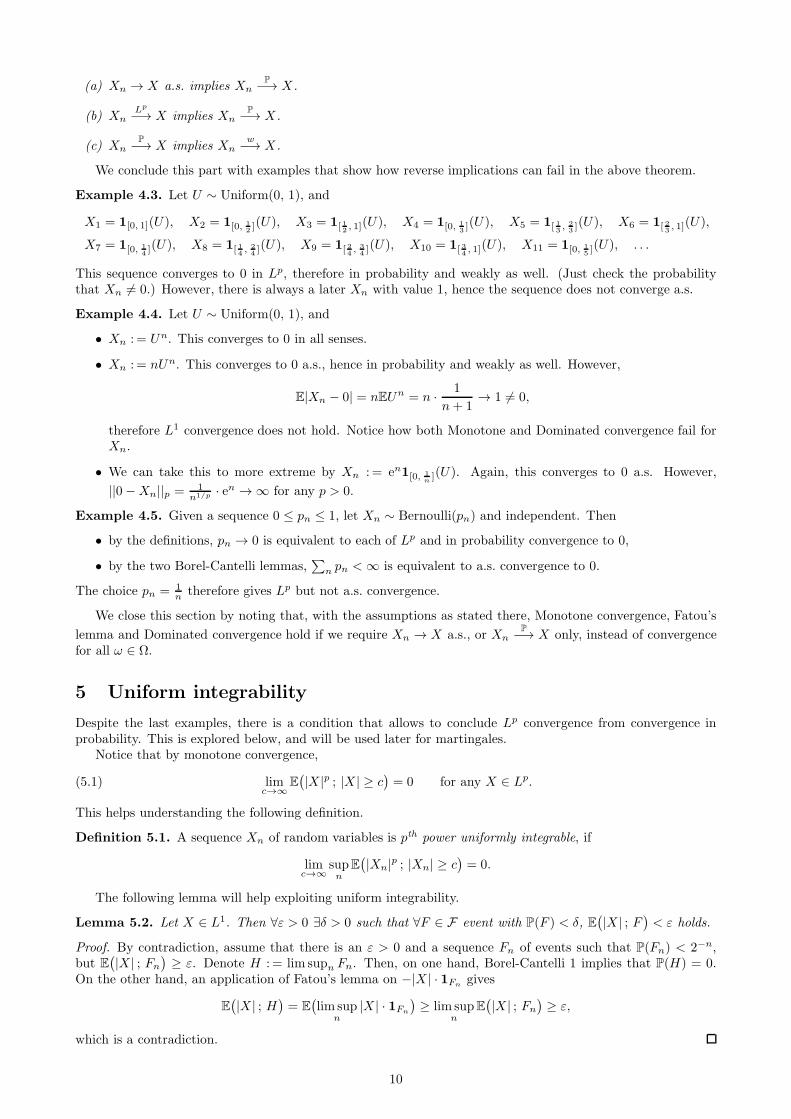
(a) Xn → X a.s. implies XnP−→ X.

(b) XnLp

−→ X implies XnP−→ X.

(c) XnP−→ X implies Xn

w−→ X.

We conclude this part with examples that show how reverse implications can fail in the above theorem.

Example 4.3. Let U ∼ Uniform(0, 1), and

X1 = 1[0, 1](U), X2 = 1[0, 12](U), X3 = 1[ 1

2, 1](U), X4 = 1[0, 1

3](U), X5 = 1[ 1

3, 23](U), X6 = 1[ 2

3, 1](U),

X7 = 1[0, 14](U), X8 = 1[ 1

4, 24](U), X9 = 1[ 2

4, 34](U), X10 = 1[ 3

4, 1](U), X11 = 1[0, 1

5](U), . . .

This sequence converges to 0 in Lp, therefore in probability and weakly as well. (Just check the probabilitythat Xn 6= 0.) However, there is always a later Xn with value 1, hence the sequence does not converge a.s.

Example 4.4. Let U ∼ Uniform(0, 1), and

• Xn : = Un. This converges to 0 in all senses.

• Xn : = nUn. This converges to 0 a.s., hence in probability and weakly as well. However,

E|Xn − 0| = nEUn = n · 1

n+ 1→ 1 6= 0,

therefore L1 convergence does not hold. Notice how both Monotone and Dominated convergence fail forXn.

• We can take this to more extreme by Xn : = en1[0, 1n ](U). Again, this converges to 0 a.s. However,

||0−Xn||p = 1n1/p · en → ∞ for any p > 0.

Example 4.5. Given a sequence 0 ≤ pn ≤ 1, let Xn ∼ Bernoulli(pn) and independent. Then

• by the definitions, pn → 0 is equivalent to each of Lp and in probability convergence to 0,

• by the two Borel-Cantelli lemmas,∑

n pn < ∞ is equivalent to a.s. convergence to 0.

The choice pn = 1n therefore gives Lp but not a.s. convergence.

We close this section by noting that, with the assumptions as stated there, Monotone convergence, Fatou’s

lemma and Dominated convergence hold if we require Xn → X a.s., or XnP−→ X only, instead of convergence

for all ω ∈ Ω.

5 Uniform integrability

Despite the last examples, there is a condition that allows to conclude Lp convergence from convergence inprobability. This is explored below, and will be used later for martingales.

Notice that by monotone convergence,

(5.1) limc→∞

E(

|X |p ; |X | ≥ c)

= 0 for any X ∈ Lp.

This helps understanding the following definition.

Definition 5.1. A sequence Xn of random variables is pth power uniformly integrable, if

limc→∞

supn

E(

|Xn|p ; |Xn| ≥ c)

= 0.

The following lemma will help exploiting uniform integrability.

Lemma 5.2. Let X ∈ L1. Then ∀ε > 0 ∃δ > 0 such that ∀F ∈ F event with P(F ) < δ, E(

|X | ; F)

< ε holds.

Proof. By contradiction, assume that there is an ε > 0 and a sequence Fn of events such that P(Fn) < 2−n,but E

(

|X | ; Fn

)

≥ ε. Denote H : = lim supn Fn. Then, on one hand, Borel-Cantelli 1 implies that P(H) = 0.On the other hand, an application of Fatou’s lemma on −|X | · 1Fn gives

E(

|X | ; H)

= E(

lim supn

|X | · 1Fn

)

≥ lim supn

E(

|X | ; Fn

)

≥ ε,

which is a contradiction.

10

We can reprove (5.1) with this lemma. If X ∈ Lp, fix Y = |X |p ∈ L1, ε > 0, and δ for this Y as in Lemma 5.2.For this δ, via Markov’s inequality, there is a large enough K, such that

P|X | ≥ K = P|X |p ≥ Kp ≤ E|X |pKp

< δ.

Then, with F = |X | ≥ K, the lemma says

E(

|X |p ; |X | ≥ K)

= E(Y ; F ) < ε.

That is, by picking large enough K, we could bring the expectation below ε. This is equivalent to (5.1).With the help of the above, we can now go from in probability convergence and uniform integrability to Lp

convergence.

Theorem 5.3. Let p ≥ 1, and suppose XnP−→ X. Then (iv) ⇒ (i) ⇔ (ii) ⇔ (iii) ⇐ (v), where

(i) XnLp

−→ X;

(ii) Xn is pth power uniformly integrable;

(iii) E|Xn|p → E|X |p;(iv) there exists a p < q < ∞, such that supn E|Xn|q < ∞;

(v) there exists a Y ∈ Lp, such that ∀n, |Xn| < Y .

Below partial proof is given to this statement.

Proof of (i) ⇒ (ii), for p = 1. Fix ε > 0, we seek K such that ∀n, E(

|Xn| ; |Xn| ≥ K)

≤ ε.By the assumed L1-convergence, there is an N such that E|X − Xn| < ε

2 whenever n > N . Lemma 5.2provides positive δ0, δ1, δ2, . . . , δN such that

∀F , if P(F ) < δ0, then E(

|X | ; F)

<ε

2, ∀F , if P(F ) < δn, then E

(

|Xn| ; F)

< ε

for 1 ≤ n ≤ N . Set δ = minδ0, δ1, . . . , δN and notice that this is still positive.When n ≤ N , define Fn = |Xn| > K, and pick K large enough that P(Fn) < δ for each 1 ≤ n ≤ N .

Notice that this is possible due to only finitely many of the Xn’s for this case. By the above, we then haveE(

|Xn| ; |Xn| ≥ K)

< ε.When n > N , we argue as follows. The assumed L1 convergence implies boundedness in L1: supr E|Xr| < ∞.

By increasing K if necessary, we can achieve

(5.2)supr E|Xr|

K< δ.

A triangle inequality gives (with common factor 1|Xn| ≥ K)

E(

|Xn| ; |Xn| ≥ K)

≤ E(

|X | ; |Xn| ≥ K)

+ E(

|Xn −X | ; |Xn| ≥ K)

≤ E(

|X | ; |Xn| ≥ K)

+ E|Xn −X |.

For the first term, take Fn = |Xn| ≥ K, and notice P(Fn) ≤ E|Xn|K < δ due to (5.2). The choice we made

with δ ≤ δ0 then bounds this term by ε2 . The second term is also bounded by ε

2 due to our initial choice of Nand n > N .

Proof of (ii) ⇒ (i), for p = 1. Define the cutoff function

ϕK(x) =

K, if x > K,

x, if −K ≤ x ≤ K,

−K, if x < −K.

Fix ε > 0 and notice that by the assumed uniform integrability and by (5.1), there is a K for which

E∣

∣ϕK(Xn)−Xn

∣

∣ <ε

3, and E

∣

∣ϕK(X)−X∣

∣ <ε

3.

Also,∣

∣ϕK(x) − ϕK(y)∣

∣ ≤ |x − y| for any x, y ∈ R, hence ϕK(Xn)P−→ ϕ(X) holds via Xn

P−→ X (check!). As

|ϕ(·)| ≤ K, Dominated convergence implies E∣

∣ϕK(Xn)− ϕ(X)∣

∣ → 0, in particular this can be brought below ε3

for large n’s. Combining via triangle inequality,

E|Xn −X | ≤ E∣

∣Xn − ϕK(Xn)∣

∣+ E∣

∣ϕK(Xn)− ϕ(X)∣

∣+ E∣

∣ϕK(X)−X∣

∣ < ε.

11

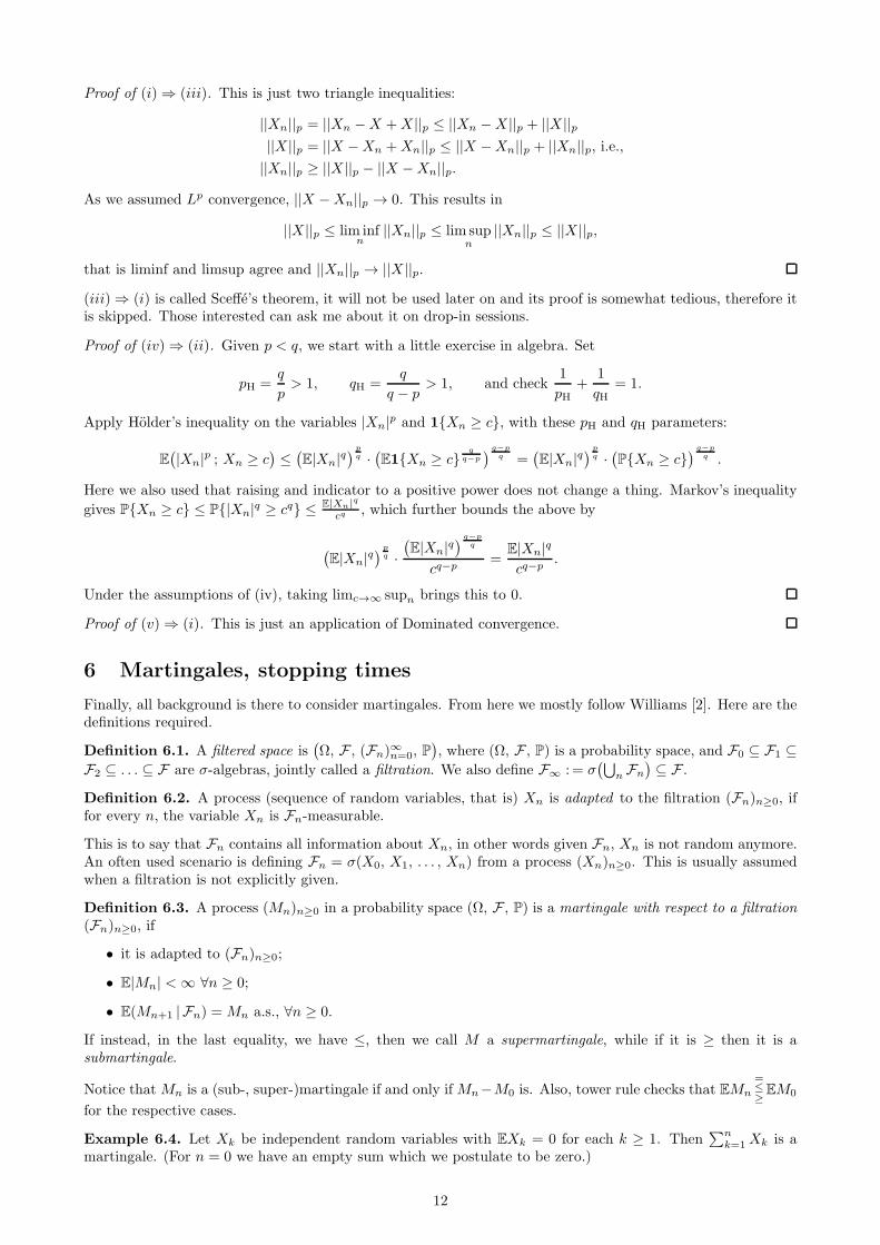
Proof of (i) ⇒ (iii). This is just two triangle inequalities:

||Xn||p = ||Xn −X +X ||p ≤ ||Xn −X ||p + ||X ||p||X ||p = ||X −Xn +Xn||p ≤ ||X −Xn||p + ||Xn||p, i.e.,||Xn||p ≥ ||X ||p − ||X −Xn||p.

As we assumed Lp convergence, ||X −Xn||p → 0. This results in

||X ||p ≤ lim infn

||Xn||p ≤ lim supn

||Xn||p ≤ ||X ||p,

that is liminf and limsup agree and ||Xn||p → ||X ||p.

(iii) ⇒ (i) is called Sceffe’s theorem, it will not be used later on and its proof is somewhat tedious, therefore itis skipped. Those interested can ask me about it on drop-in sessions.

Proof of (iv) ⇒ (ii). Given p < q, we start with a little exercise in algebra. Set

pH =q

p> 1, qH =

q

q − p> 1, and check

1

pH+

1

qH= 1.

Apply Holder’s inequality on the variables |Xn|p and 1Xn ≥ c, with these pH and qH parameters:

E(

|Xn|p ; Xn ≥ c)

≤(

E|Xn|q)

pq ·

(

E1Xn ≥ c qq−p

)

q−pq =

(

E|Xn|q)

pq ·

(

PXn ≥ c)

q−pq .

Here we also used that raising and indicator to a positive power does not change a thing. Markov’s inequality

gives PXn ≥ c ≤ P|Xn|q ≥ cq ≤ E|Xn|q

cq , which further bounds the above by

(

E|Xn|q)

pq ·

(

E|Xn|q)

q−pq

cq−p=

E|Xn|qcq−p

.

Under the assumptions of (iv), taking limc→∞ supn brings this to 0.

Proof of (v) ⇒ (i). This is just an application of Dominated convergence.

6 Martingales, stopping times

Finally, all background is there to consider martingales. From here we mostly follow Williams [2]. Here are thedefinitions required.

Definition 6.1. A filtered space is(

Ω, F , (Fn)∞n=0, P

)

, where (Ω, F , P) is a probability space, and F0 ⊆ F1 ⊆F2 ⊆ . . . ⊆ F are σ-algebras, jointly called a filtration. We also define F∞ : = σ

(⋃

n Fn

)

⊆ F .

Definition 6.2. A process (sequence of random variables, that is) Xn is adapted to the filtration (Fn)n≥0, iffor every n, the variable Xn is Fn-measurable.

This is to say that Fn contains all information about Xn, in other words given Fn, Xn is not random anymore.An often used scenario is defining Fn = σ(X0, X1, . . . , Xn) from a process (Xn)n≥0. This is usually assumedwhen a filtration is not explicitly given.

Definition 6.3. A process (Mn)n≥0 in a probability space (Ω, F , P) is a martingale with respect to a filtration(Fn)n≥0, if

• it is adapted to (Fn)n≥0;

• E|Mn| < ∞ ∀n ≥ 0;

• E(Mn+1 | Fn) = Mn a.s., ∀n ≥ 0.

If instead, in the last equality, we have ≤, then we call M a supermartingale, while if it is ≥ then it is asubmartingale.

Notice that Mn is a (sub-, super-)martingale if and only if Mn−M0 is. Also, tower rule checks that EMn

=≤≥EM0

for the respective cases.

Example 6.4. Let Xk be independent random variables with EXk = 0 for each k ≥ 1. Then∑n

k=1 Xk is amartingale. (For n = 0 we have an empty sum which we postulate to be zero.)

12

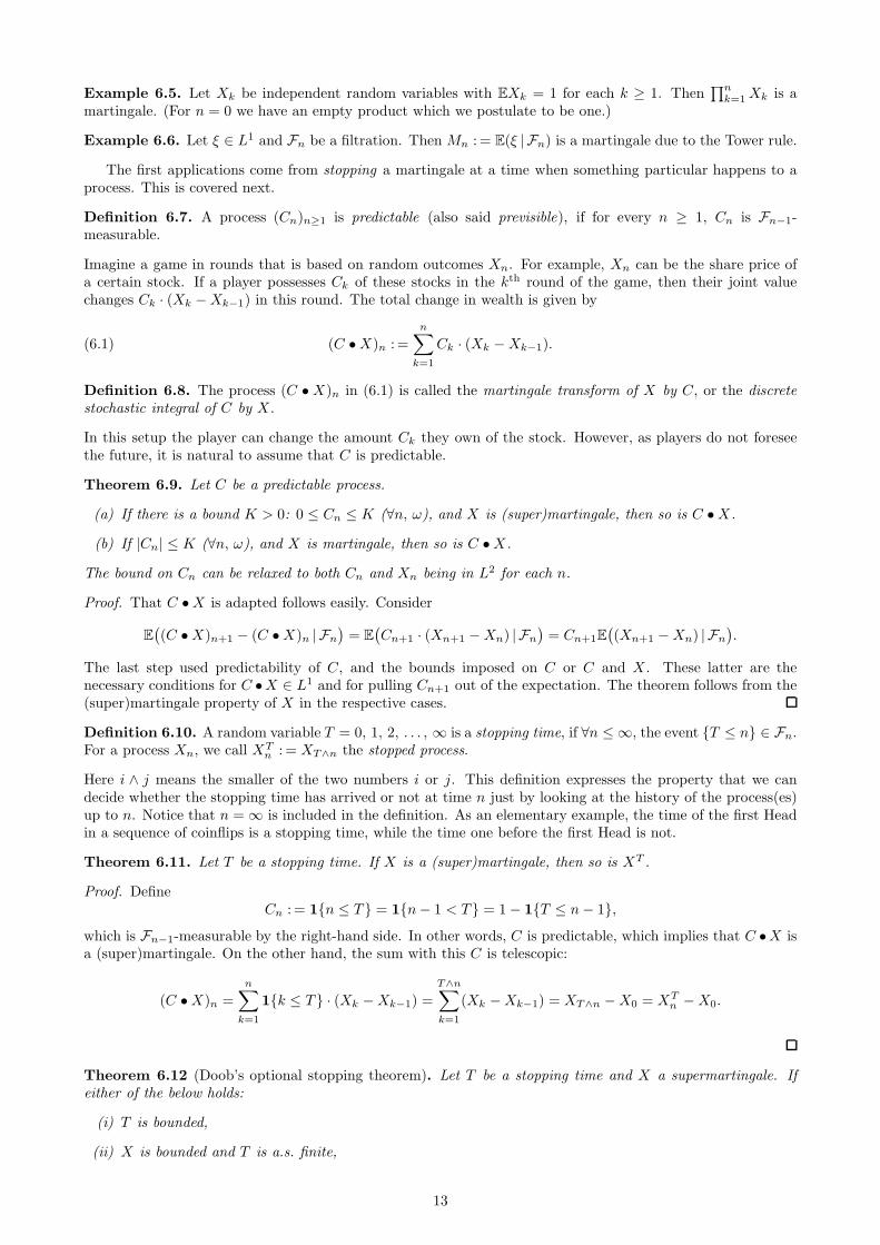
Example 6.5. Let Xk be independent random variables with EXk = 1 for each k ≥ 1. Then∏n

k=1 Xk is amartingale. (For n = 0 we have an empty product which we postulate to be one.)

Example 6.6. Let ξ ∈ L1 and Fn be a filtration. Then Mn : = E(ξ | Fn) is a martingale due to the Tower rule.

The first applications come from stopping a martingale at a time when something particular happens to aprocess. This is covered next.

Definition 6.7. A process (Cn)n≥1 is predictable (also said previsible), if for every n ≥ 1, Cn is Fn−1-measurable.

Imagine a game in rounds that is based on random outcomes Xn. For example, Xn can be the share price ofa certain stock. If a player possesses Ck of these stocks in the kth round of the game, then their joint valuechanges Ck · (Xk −Xk−1) in this round. The total change in wealth is given by

(6.1) (C •X)n : =

n∑

k=1

Ck · (Xk −Xk−1).

Definition 6.8. The process (C •X)n in (6.1) is called the martingale transform of X by C, or the discretestochastic integral of C by X .

In this setup the player can change the amount Ck they own of the stock. However, as players do not foreseethe future, it is natural to assume that C is predictable.

Theorem 6.9. Let C be a predictable process.

(a) If there is a bound K > 0: 0 ≤ Cn ≤ K (∀n, ω), and X is (super)martingale, then so is C •X.

(b) If |Cn| ≤ K (∀n, ω), and X is martingale, then so is C •X.

The bound on Cn can be relaxed to both Cn and Xn being in L2 for each n.

Proof. That C •X is adapted follows easily. Consider

E(

(C •X)n+1 − (C •X)n | Fn

)

= E(

Cn+1 · (Xn+1 −Xn) | Fn

)

= Cn+1E(

(Xn+1 −Xn) | Fn

)

.

The last step used predictability of C, and the bounds imposed on C or C and X . These latter are thenecessary conditions for C •X ∈ L1 and for pulling Cn+1 out of the expectation. The theorem follows from the(super)martingale property of X in the respective cases.

Definition 6.10. A random variable T = 0, 1, 2, . . . , ∞ is a stopping time, if ∀n ≤ ∞, the event T ≤ n ∈ Fn.For a process Xn, we call XT

n : = XT∧n the stopped process.

Here i ∧ j means the smaller of the two numbers i or j. This definition expresses the property that we candecide whether the stopping time has arrived or not at time n just by looking at the history of the process(es)up to n. Notice that n = ∞ is included in the definition. As an elementary example, the time of the first Headin a sequence of coinflips is a stopping time, while the time one before the first Head is not.

Theorem 6.11. Let T be a stopping time. If X is a (super)martingale, then so is XT .

Proof. DefineCn : = 1n ≤ T = 1n− 1 < T = 1− 1T ≤ n− 1,

which is Fn−1-measurable by the right-hand side. In other words, C is predictable, which implies that C •X isa (super)martingale. On the other hand, the sum with this C is telescopic:

(C •X)n =

n∑

k=1

1k ≤ T · (Xk −Xk−1) =

T∧n∑

k=1

(Xk −Xk−1) = XT∧n −X0 = XTn −X0.

Theorem 6.12 (Doob’s optional stopping theorem). Let T be a stopping time and X a supermartingale. Ifeither of the below holds:

(i) T is bounded,

(ii) X is bounded and T is a.s. finite,

13

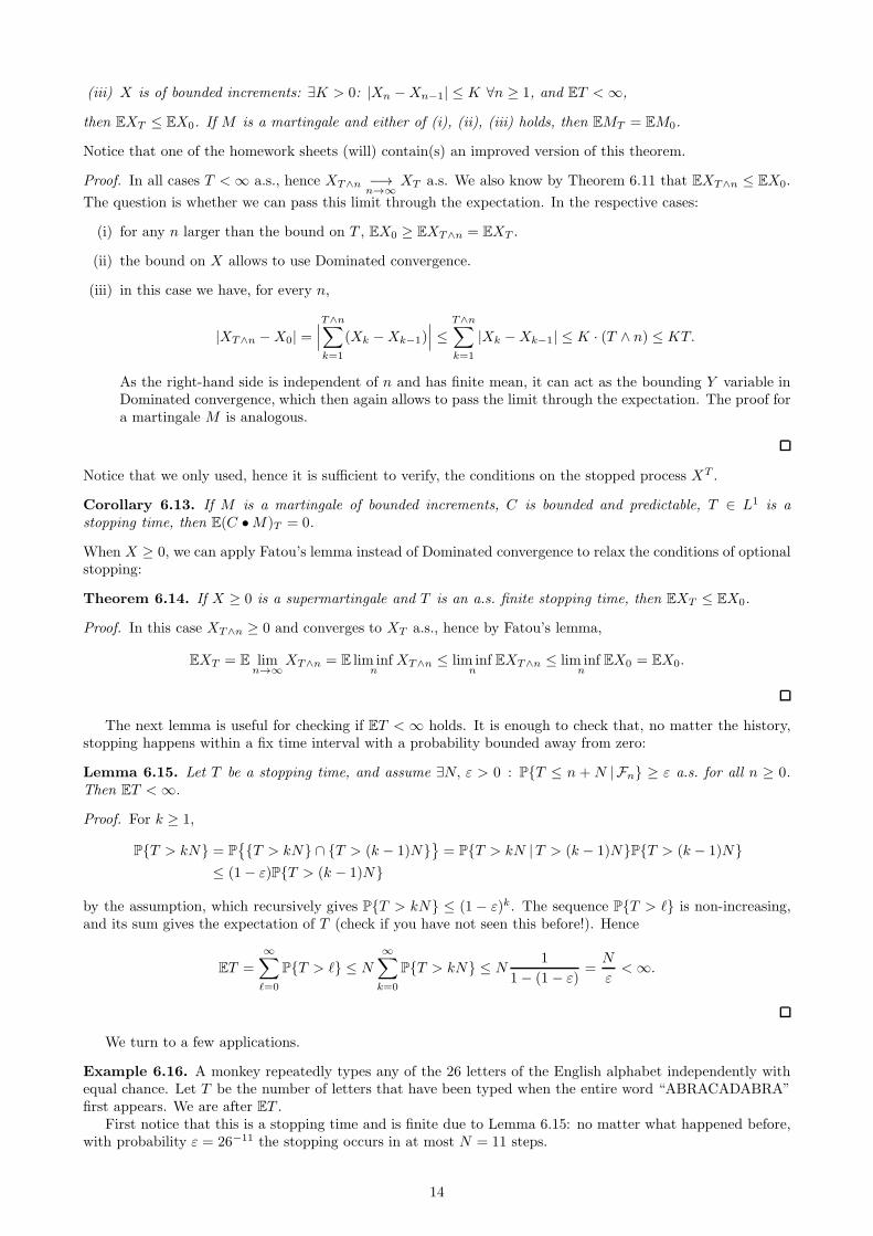
(iii) X is of bounded increments: ∃K > 0: |Xn −Xn−1| ≤ K ∀n ≥ 1, and ET < ∞,

then EXT ≤ EX0. If M is a martingale and either of (i), (ii), (iii) holds, then EMT = EM0.

Notice that one of the homework sheets (will) contain(s) an improved version of this theorem.

Proof. In all cases T < ∞ a.s., hence XT∧n −→n→∞

XT a.s. We also know by Theorem 6.11 that EXT∧n ≤ EX0.

The question is whether we can pass this limit through the expectation. In the respective cases:

(i) for any n larger than the bound on T , EX0 ≥ EXT∧n = EXT .

(ii) the bound on X allows to use Dominated convergence.

(iii) in this case we have, for every n,

|XT∧n −X0| =∣

∣

∣

T∧n∑

k=1

(Xk −Xk−1)∣

∣

∣≤

T∧n∑

k=1

|Xk −Xk−1| ≤ K · (T ∧ n) ≤ KT.

As the right-hand side is independent of n and has finite mean, it can act as the bounding Y variable inDominated convergence, which then again allows to pass the limit through the expectation. The proof fora martingale M is analogous.

Notice that we only used, hence it is sufficient to verify, the conditions on the stopped process XT .

Corollary 6.13. If M is a martingale of bounded increments, C is bounded and predictable, T ∈ L1 is astopping time, then E(C •M)T = 0.

When X ≥ 0, we can apply Fatou’s lemma instead of Dominated convergence to relax the conditions of optionalstopping:

Theorem 6.14. If X ≥ 0 is a supermartingale and T is an a.s. finite stopping time, then EXT ≤ EX0.

Proof. In this case XT∧n ≥ 0 and converges to XT a.s., hence by Fatou’s lemma,

EXT = E limn→∞

XT∧n = E lim infn

XT∧n ≤ lim infn

EXT∧n ≤ lim infn

EX0 = EX0.

The next lemma is useful for checking if ET < ∞ holds. It is enough to check that, no matter the history,stopping happens within a fix time interval with a probability bounded away from zero:

Lemma 6.15. Let T be a stopping time, and assume ∃N, ε > 0 : PT ≤ n + N | Fn ≥ ε a.s. for all n ≥ 0.Then ET < ∞.

Proof. For k ≥ 1,

PT > kN = P

T > kN ∩ T > (k − 1)N

= PT > kN |T > (k − 1)NPT > (k − 1)N≤ (1− ε)PT > (k − 1)N

by the assumption, which recursively gives PT > kN ≤ (1 − ε)k. The sequence PT > ℓ is non-increasing,and its sum gives the expectation of T (check if you have not seen this before!). Hence

ET =

∞∑

ℓ=0

PT > ℓ ≤ N

∞∑

k=0

PT > kN ≤ N1

1− (1 − ε)=

N

ε< ∞.

We turn to a few applications.

Example 6.16. A monkey repeatedly types any of the 26 letters of the English alphabet independently withequal chance. Let T be the number of letters that have been typed when the entire word “ABRACADABRA”first appears. We are after ET .

First notice that this is a stopping time and is finite due to Lemma 6.15: no matter what happened before,with probability ε = 26−11 the stopping occurs in at most N = 11 steps.

14

To proceed, we add a gambling process to this problem. Before each hit of a new letter, a new gamblerarrives and bets £1 on the letter “A”. If the new letter is something else, the gambler looses their bet and exitsthe game. If the new letter is “A”, then the gambler receives £26, which they all bet on the next letter being“B”. If this next letter is something else, all bet is lost and the gambler exits the game. If this next letter is“B”, then the gambler receives £262, which they all bet on the third letter being “R”, and so on. If the gamblerwins all the way down to “ABRACADABRA”, the gambler exits the game with wealth £2611 and T becomesthe total number of letters typed at this point. Otherwise the gambler looses all their money and exits thegame. Also, new gamblers arrive at each step and start the same betting strategy. Denote by Xn the combinedwealth of all gamblers who are in play after the nth letter has been typed. We claim that Mn : = Xn − n is amartingale.

To check this, notice that Mn is adapted to the natural filtration generated by the monkey, and is boundedfor any given n, hence is in L1. The martingale property is checked by first observing that the expected wealthof a gambler already in play does not change. That is because their bet is lost with probability 25

26 and multipliedby 26 with probability 1

26 , hence the mean value stays. A gambler already out of play stays with their 0 wealthso that doesn’t change either. However, a new gambler arrives and their expected wealth after a flip is 26 · 1

26 = 1which adds to the conditional expectation of Xn+1. Therefore,

E(Mn+1 | Fn) = E(Xn+1 | Fn)− (n+ 1) = Xn + 1− (n+ 1) = Mn.

Notice that EM1 = EX1 − 1 = 0, hence we can extend the definition by M0 = 0.The stopped martingale MT is of bounded increments, and ET < ∞, hence Optional stopping applies and

gives0 = M0 = EMT = EXT − ET.

It remains to calculate XT . At the time of stopping, there are only three gamblers in play. The one who came attime T − 11 has wealth 2611. Less lucky is the gambler who arrived at T − 4; they successfully bet on “ABRA”and have £264. Finally, the gambler who just arrived at T and bet on “A” has £26. Thus,

ET = EXT = XT = 2611 + 264 + 26 ≃ 3.7 · 1015.

Notice how repetitions in “ABRACADABRA” increase ET (why?).

Example 6.17. LetXk be iid.±1-valued with equal chance. The sum Sn =∑n

k=1 Xk is called simple symmetricrandom walk (SSRW). Empty sums are zero, hence S0 = 0. Then Sn is a martingale, and

T : = infn : Sn = 1

is a stopping time in the natural filtration of the walk. We will check in Example 6.18 that T is a.s. finite, andST = 1 a.s. Also, EST∧n = ES0 = 0 from the martingale property, as seen in Theorem 6.11. However, theconditions of Optional stopping are not met, and

1 = EST 6= ES0 = 0.

In particular this shows via case (iii) of Optional stopping that ET = ∞ since Sn is of bounded increment.

Example 6.18. Consider the SSRW and the stopping time T as in Example 6.17. We show T < ∞ a.s., andeven calculate its moment generating function. Finiteness of T implies recurrence of SSRW.

For any θ > 0, the process

Mθn : =

eθSn

(cosh θ)n

is a martingale. It is clearly adapted and finite for each n, and the martingale property works out:

E(

Mθn+1 | Fn

)

=E(

eθ(Sn+Xn+1) | Fn

)

(cosh θ)n+1=

eθSn

(cosh θ)n+1· e

θ + e−θ

2=

eθSn

(cosh θ)n= Mθ

n.

We cannot rule out T = ∞. However, in this case we know Sn ≤ 0 for each n, hence

0 ≤ Mθn ≤ eθ·0

(cosh θ)n−→n→∞

0

by cosh θ > 1. On the event T = ∞ we therefore define MθT = 0 and have Mθ

T∧n = Mθn −→

n→∞Mθ

T . We also

have MθT∧n −→

n→∞Mθ

T on T < ∞.By definition of T ,

MθT∧n =

eθST∧n

(cosh θ)T∧n≤ eθ

(cosh θ)T∧n≤ eθ,

15

which is a bound independent of n, hence dominated convergence applies on the above limit:

1 = limn→∞

EMθT∧n = E lim

n→∞Mθ

T∧n = EMθT = E(Mθ

T ; T < ∞) = E

( eθST

(cosh θ)T; T < ∞

)

= E

( eθ

(cosh θ)T; T < ∞

)

= E

( eθ

(cosh θ)T

)

,

where the martingale property EMθT∧n = Mθ

0 = 1, then MθT = 0 on T = ∞, then ST = 1 on T < ∞, finally

cosh θ > 1 were used. From this we conclude

(6.2) E

( 1

(cosh θ)T

)

= e−θ.

Next we take θ ց 0, which makes cosh θ ց 1. If T = ∞ then 1(cosh θ)T = 0 for any θ > 0, hence so is its

limit. However, if T < ∞ then the limit is 1. Together,

limθց0

1

(cosh θ)T= 1T < ∞.

As the bound 0 ≤ 1(cosh θ)T ≤ 1 holds no matter the value of T , we can apply dominated convergence on the

above limit:

1 = limθց0

e−θ = limθց0

E

( 1

(cosh θ)T

)

= E

(

limθց0

1

(cosh θ)T

)

= E1T < ∞ = PT < ∞,

which was our goal.Substitute 0 < α = 1

cosh θ < 1 into (6.2) and solve this substitution for e−θ to obtain (check!) the generatingfunction for the random variable T

EαT =1−

√1− α2

α.

7 Martingale convergence

This section gives an introduction to yet another strength of the martingale property: convergence under rathergeneral assumptions. We start with examining upcrossings :

Definition 7.1. Fix a < b real numbers and let Xn be a process. The upcrossing number until N is defined as

UN [a, b] : = maxk : ∃0 ≤ s1 < t1 < s2 < t2 < · · · < sk < tk ≤ N with Xsi < a, Xti > b for all 1 ≤ i ≤ k.

This definition counts what the name suggests: how many times the process increases from below level a toabove level b before time N . To capture these increments, we also define

C0 : = 0, Cn : = 1Cn−1 = 11Xn−1 ≤ b+ 1Cn−1 = 01Xn−1 < a (n ≥ 1).

Think about Cn as an on-off switch: once it is on (Cn−1 = 1), it stays on unless X exceeds level b. Once itis off (Cn−1 = 0), it stays off until X descends below level a. Notice that if Xn is adapted, then this Cn ispredictable. Let

Yn : = (C •X)n =

n∑

k=1

(Xk −Xk−1)Ck.

This captures the increments of X during the on periods of C. It then follows that

YN ≥ (b − a) · UN [a, b]− (XN − a)−.

To see this notice that any upcrossing is of increment at least b− a, all of which is captured by YN . However, ifX descends below a after the last upcrossing, that is also captured by YN and might contribute with a negativesign. This is taken care of by the last term.

Lemma 7.2 (Doob’s upcrossing lemma). If Xn is a supermartingale, then (b− a)EUN [a, b] ≤ E(XN − a)−.

Proof. By Theorem 6.9, Yn is a supermartingale, hence EYN ≤ 0.

Corollary 7.3. Let a < b, and let Xn be a supermartingale that is bounded in L1. (That is, supn E|Xn| < ∞.)Then

(b− a)EU∞[a, b] ≤ |a|+ supm

E|Xm| < ∞.

In particular, U∞[a, b] is a.s. finite.

16

Proof. As UN [a, b] ≥ 0 is monotone in N , we have

(b− a)EU∞[a, b] = (b− a)E limN

UN [a, b] = (b− a) limN

EUN [a, b] ≤ limN

E(XN − a)−

by monotone convergence. To finish the proof,

E(XN − a)− ≤ E|XN − a| ≤ E|XN |+ |a| ≤ |a|+ supm

E|Xm|,

and the right-hand side is independent of N .

Theorem 7.4 (Doob’s forward convergence theorem). Let Xn be a supermartingale that is bounded in L1.Then X∞ : = limn Xn exists a.s. and is finite.

Proof.

Xn does not converge = lim infn

Xn < lim supn

Xn =⋃

a<ba,b∈Q

lim infn

Xn < a < b < lim supn

Xn

⊆⋃

a<ba,b∈Q

U∞[a, b] = ∞.

The right-hand side is a countable union of zero probability events, has zero probability itself.To see that the limit is a.s. finite, use Fatou’s lemma:

E|X∞| = E lim infn

|Xn| ≤ lim infn

E|Xn| ≤ supn

E|Xn| < ∞,

which implies |X∞| < ∞ a.s.

Notice that if Xn ≥ 0 is a supermartingale, then L1-boundedness is automatic: E|Xn| = EXn ≤ EX0.Finally, we have a bit to say about L2-martingales. The scalar product of L2-random variables X and Y is

defined by 〈X, Y 〉 : = E(XY ). Indeed check that this defines a scalar product. If Mn is an L2-martingale, andk ≤ m < n, then Mn − Mm is orthogonal to Fk of the filtration. Namely, for any Y Fk-measurable randomvariable

〈Mn−Mm, Y 〉 = E(

(Mn−Mm)Y)

= EE(

(Mn−Mm)Y | Fk

)

= E(

Y E(Mn−Mm | Fk))

= E(

Y ·(Mk−Mk))

= 0.

In particular, increments of an L2-martingale in disjoint time intervals are orthogonal: for ℓ < k ≤ m < n,〈Mn −Mm, Mk −Mℓ〉 = 0. Another way of stating this is that these increments are uncorrelated. This is themain observation used in the next theorem.

Theorem 7.5. An L2 martingale Mn is bounded in L2 if and only if∑∞

k=1 E(Mk −Mk−1)2 < ∞. In this case

Mn → M∞ a.s. and in L2.

Proof. Due to the orthogonal increments as above, all cross terms of the square below have zero mean, and thefollowing Pythagorean theorem holds:

EM2n = E

(

M0 +

n∑

k=1

(Mk −Mk−1))2

= EM20 +

n∑

k=1

E(Mk −Mk−1)2 ≤ EM2

0 +

∞∑

k=1

E(Mk −Mk−1)2.

This proves the first statement.If Mn is bounded in L2, then it is also bounded in L1 by Ljapunov’s inequality, and the forward convergence

theorem provides the a.s. limit. To see the L2 convergence, use Fatou’s lemma and the Pythagorean theoremas

E(M∞ −Mn)2 = E lim

r→∞(Mn+r −Mn)

2 ≤ lim infr

E(Mn+r −Mn)2 = lim inf

r

n+r∑

k=n+1

E(Mk −Mk−1)2

=

∞∑

k=n+1

E(Mk −Mk−1)2 −→

n→∞0

due to finiteness of the infinite sum.

17

8 Uniformly integrable martingales

Uniform integrability gives further powerful tools with martingales:

Theorem 8.1. Let Mn be a uniformly integrable martingale. Then M∞ = limn→∞ Mn exists a.s. and in L1,and Mn = E(M∞ | Fn) a.s.

Proof. Due to uniform integrability, we can pick a c > 0 for which supn E(|Mn| ; |Mn| ≥ c) ≤ 1. Then,

E|Mn| = E(|Mn| ; |Mn| ≥ c) + E(|Mn| ; |Mn| < c) ≤ 1 + c,

where we used the simple algebraic fact that |x| · 1|x| < c ≤ c for any real x. As the right-hand sideis independent of n, it follows that Mn is bounded in L1, thus converges a.s. to a finite limit by Doob’sforward convergence. That implies convergence in probability, which in turn gives L1 convergence when uniformintegrability is added (Theorem 5.3).

For the last bit, fix r > n > 0, F ∈ Fn:

|E(Mn ; F )−E(M∞ ; F )| = |E(Mr ; F )−E(M∞ ; F )| = |E(Mr−M∞ ; F )| ≤ E(

|Mr−M∞| ; F)

≤ E|Mr−M∞|

a.s., where first the martingale property (check how!), then Jensen’s inequality on the | · | function was used.By the L1 convergence, the right-hand side goes to 0 as r → ∞. As the left-hand side has no r in it, it istherefore zero: E(Mn ; F ) = E(M∞ ; F ). This proves Mn = E(M∞ | Fn) a.s. due to the Kolmogorov definitionof conditional expectations and Mn being Fn-measurable.

The next theorem is the reverse statement in some sense.

Theorem 8.2 (Levy’s upwards theorem). Let ξ ∈ L1, (Fn)n be a filtration, and Mn : = E(ξ | Fn) (this is welldefined almost everywhere). Then Mn is a uniformly integrable martingale, Mn converges a.s. and in L1 to alimit M∞, and M∞ = E(ξ | F∞) a.s.

Proof. The proof has three parts.1. That Mn is a martingale is a simple application of the Tower rule.2. Next we show that Mn is uniformly integrable. Fix ε > 0 and δ > 0 for ξ as in Lemma 5.2. Then pick

K > E|ξ|δ . An application of Markov’s inequality, Jensen’s inequality on the conditional expectation, then the

Tower rule shows

P|Mn| ≥ K ≤ E|Mn|K

=E∣

∣E(ξ | Fn)∣

∣

K≤ EE

(

|ξ|∣

∣Fn

)

K=

E|ξ|K

< δ,

making |Mn| ≥ K a suitable event for Lemma 5.2. We apply this lemma in the last step below, followingconditional Jensen again, the fact that |Mn| ≥ K ∈ Fn and the Tower rule:

E[|Mn| ; |Mn| ≥ K] = E[∣

∣E(ξ | Fn)∣

∣ ; |Mn| ≥ K]

≤ E[

E(

|ξ|∣

∣Fn

)

; |Mn| ≥ K]

= EE(

|ξ| ; |Mn| ≥ K∣

∣Fn

)

= E(

|ξ| ; |Mn| ≥ K)

≤ ε.

The right-hand side has no n, hence uniform integrability is proved. This implies existence of the limit M∞.3. We need to show that this limit M∞ a.s. coincides with η : = E(ξ | F∞). We do this for the case ξ > 0,

otherwise the difference ξ = ξ+ − ξ− then provides the general proof. For any set F ∈ F∞, let

Q1(F ) : = E(η ; F ) and Q2(F ) : = E(M∞ ; F ),

these are measures on (Ω, F∞). If F ∈ Fn, then Tower rules, measurability (recall Fn ⊆ F∞), and Mn =E(M∞ | Fn) from the previous theorem imply

Q1(F ) = E(η ; F ) = E(

E(ξ | F∞) ; F)

= EE(ξ ; F | F∞) = E(ξ ; F )

= EE(ξ ; F | Fn) = E(

E(ξ | Fn) ; F)

= E(Mn ; F )

= E(

E(M∞ | Fn) ; F)

= EE(M∞ ; F | Fn) = E(M∞ ; F ) = Q2(F ).

This shows that Q1 agrees with Q2 on⋃

n Fn = F∞. Since η > M∞ ∈ F∞,

0 = Q1η > M∞ −Q2η > M∞ = E(η −M∞ ; η > M∞),

therefore Pη > M∞ = 0. In a similar way Pη < M∞ = 0, which completes the proof.

Next we prove an important theorem in probability using the machinery built up so far.

18

Definition 8.3. Let X1, X2, . . . be independent random variables, and τn : = σ(Xn+1, Xn+2, . . . ). The tailσ-algebra is τ : =

⋂

n τn.

An event in τ is τn-measurable for every n. In other words, it does not depend on any finite number of changesin the sequence X1, X2, . . ..

Theorem 8.4 (Kolmogorov’s 0-1 law). The tail σ-algebra of independent variables is trivial. That is, with theabove definition, for any F ∈ τ we have P(F ) = 0 or 1.

It is important here that the random variables are independent.

Proof. Let, as before, Fn = σ(X1, X2, . . . ) and F ∈ τ . Define η = 1F . As F ∈ τ ⊆ F∞, η is F∞-measurable,and is of course in L1. Add Levy’s upwards theorem:

η = E(η | F∞) = limn→∞

E(η | Fn).

However, F ∈ τ ⊆ τn, which is independent of Fn, as these are generated by a disjoint set of independentrandom variables. It follows that

1F = η = limn→∞

E(η | Fn) = limn→∞

Eη = Eη = P(F ),

which shows P(F ) is either 0 or 1.

Example 8.5. For a SSRW Sn =∑n

k=1 Xk, let F : = Sn

n → v be the event that the walk has asymptotic

velocity v. Changing any finite number of the iid. Xk’s does not influence the liminf, nor the limsup, of Sn

n ,hence F is in the tail σ-algebra of the Xk’s. It follows that F is trivial, has either probability 0 or 1. Indeed,the Strong law of large numbers states that P(F ) = 1 when v = 0, and zero in all other cases.

Recall that a filtration is an increasing system of σ-algebras and a natural interpretation is the expandinginformation collected from observing a process starting at time zero. In what follows we still have a filtration,but the σ-algebras are indexed up to time −1, rather than starting from time 0 as before. Accordingly, the limitis taken as the σ-algebras decrease, rather than increase which is what has been done so far. An applicationfollows further down.

Theorem 8.6 (Levy’s downward theorem). Let G−n, n ≥ 1, be σ-algebras with

G−n ⊆ G−n+1 ⊆ G−n+2 ⊆ . . . ⊆ G−1, and G−∞ : =

∞⋂

n=1

G−n.

Let γ ∈ L1, and M−n : = E(γ | G−n). Then M−∞ : = limn→∞ M−n exists a.s. and in L1, and M−∞ = E(γ | G−∞)a.s.

Proof. The martingale property E(M−n+1 | G−n) = M−n is checked the very same way as in Example 6.6, exceptthe time index is negative.

Uniform integrability works the same way as in Levy’s upward theorem. This implies L1-boundedness, andthe upcrossing proof works as well to show a.s. convergence. Together with uniform integrability, L1 convergencefollows.

Finally, to show M−∞ = E(γ | G−∞) a.s., fix r > 0 and an event G ∈ G−∞ ⊆ G−r. Then

E(γ ; G) = EE(γ ; G | G−r) = E(

E(γ | G−r) ; G)

= E(M−r ; G).

Further, due to Jensen’s inequality and the L1 convergence,

|E(M−r ; G)− E(M−∞ ; G)| =∣

∣E(M−r −M−∞ ; G)∣

∣ ≤ E(

|M−r −M−∞| ; G)

≤ E|M−r −M−∞| −→r→∞

0.

Hence E(γ ; G) = E(M−∞ ; G), and M−∞ = E(γ | G−∞) a.s. follows from M−∞ being G−∞-measurable and theKolmogorov definition of conditional expectations.

As an application, here is the proof of the Strong law of large numbers using martingales.

Theorem 8.7 (Strong law of large numbers). Let Xk be iid. random variables in L1, and Sn =∑n

k=1 Xk.Then Sn

n → EX1 a.s. and in L1.

19

Proof. Let G−n = σ(Sn, Sn+1, . . . ), and notice that this system satisfies the conditions of the Downwardtheorem. Notice also that due to independence and the structure of Sn,

G−n = σ

σ(Sn), σ(Xn+1, Xn+2, . . . )

,

where the σ-algebras σ(Sn), σ(Xn+1, Xn+2, . . . ) are independent. This is to say that the process of Sm’s,m ≥ n from time n is determined by Sn and, independently, Xk’s for k > n. It follows by symmetry (check!)that

M−n : = E(X1 | G−n) = E(

X1 |σ(Sn))

=Sn

n.

Levy’s downward theorem applies on this martingale, and gives the existence of the a.s. and L1 limit M−∞.All that is left is to identify what this limit is. To this order notice that M−∞ = limn→∞ M−n = limn→∞

Sn

na.s. (one can instead use limsup here to make sure it is defined surely) does not depend on changes made onany finitely many of the Xk’s. It is therefore in the tail σ-algebra of the iid. sequence, which is trivial byKolmogorov’s 0-1 law. For any c ∈ R, PM−∞ = c is therefore 0 or 1. However, it cannot be 0 for every c,there exists a non-random value which M−∞ takes a.s. and, due to EM−∞ = EM−1 = EX1, this value can onlybe EX1.

9 Doob’s submartingale inequality

We continue with yet another important property of (sub)martingales. Compare the below with Markov’sinequality.

Theorem 9.1 (Doob’s submartingale inequality). Let Zn ≥ 0 be a submartingale. Then for every c > 0 realand n > 0 integer,

P

supk≤n

Zk ≥ c

≤ E(

Zn ; supk≤n Zk ≥ c)

c≤ EZn

c.

Since we are looking at a finite number of values, ‘max’ would be appropriate instead of ‘sup’. However, ‘sup’is the usual formulation as it also works for the continuous time version of the theorem.

Proof. If the event F : =

supk≤n Zk ≥ c

occurs, then there must be a first instance of k where Zk ≥ c. Thisis captured by the disjoint union

F =

n⋃

k=0

Fk, where

F0 : = Z0 ≥ c,

Fk : =

k−1⋂

i=0

Zi < c ∩ Zk ≥ c (k > 0).

Notice that Fk ∈ Fk, hence the submartingale property gives, for k ≤ n,

E(Zn ; Fk) = EE(

(Zn ; Fk) | Fk

)

= E(

E(Zn | Fk) ; Fk

)

≥ E(

E(Zk | Fk) ; Fk

)

= EE(

(Zk ; Fk) | Fk

)

= E(Zk ; Fk).

The event Fk implies Zk ≥ c, hence we can proceed by

E(Zn ; Fk) ≥ E(Zk ; Fk) ≥ cP(Fk).

Summing this in k proves the theorem via the disjoint union above.

Submartingales occur more often than one would first think. Let Mn be a martingale, g a convex function,and assume E|g(Mn)| < ∞ for each n. Then by Jensen’s inequality,

E(

g(Mn+1) | Fn

)

≥ g(

E(Mn+1 | Fn))

= g(Mn),

hence g(Mn) is a submartingale.

Example 9.2. A total of n people queue up to buy one ticket each for a small performance with n seats in thetheatre. The price is one pound, and each person independently, with equal chance either has exact change,or a two pound coin in which case a one pound coin change is needed from the cashier. The cashier starts theservice with m one pound coins. We seek an upper bound on the probability that the cashier runs out of onepound coins at some point while serving this queue.

Set Xi to be 1 if person i has one pound, and −1 if they have a two pound coin. Then Sk : =∑k

i=1 Xi is thechange in the number of one pound coins with the cashier due to serving the first k customers. It is a SSRWhence a martingale, and the cashier runs out of one pound coins iff m+min1≤k≤n Sk < 0.

20

A non-negative submartingale is produced by taking square (a convex function) of Sk. Hence, the probabilityof the cashier running out of change is bounded by

P

min1≤k≤n

Sk < −m

≤ P

sup1≤k≤n

S2k ≥ (m+ 1)2

≤ ES2n

(m+ 1)2=

n

(m+ 1)2.

As an example, n = 100 and m = 30 already gives a bound of cca 10%.

10 A discrete Black-Scholes option pricing formula

As an application, a very simple version of the option pricing formula is presented, still following Williams [2].First, the probability space that will govern the stock market is assumed in this form:

(10.1) Ω = ω1, ω2, . . . , ωN, where ωn =

+ 1, with probability p,

− 1, with probability 1− p,

independently for different n’s. This generates the natural filtration Fn = σω1, . . . , ωn.Stocks have value Sn, while bonds have value Bn per unit on day n, 0 ≤ n ≤ N . We have An stocks, and

Vn bonds in the morning of day n, so our total wealth is AnSn + VnBn. During the day, we are allowed toexchange these, and by the evening of day n we might have An+1 stocks and Vn+1 bonds. However, the totalwealth during transactions must be conserved:

(10.2) Xn : = AnSn + VnBn = An+1Sn + Vn+1Bn.

Overnight, the values change from Sn to Sn+1 for stocks, and from Bn to Bn+1 for bonds. Bonds are not veryexciting, their value is deterministic, Bn = (1 + r)nB0 with a fixed −1 < r < ∞, which one can also write as

Bn −Bn−1 = rBn−1.

Stocks, on the other hand, will change randomly. With −1 < a < r < b < ∞ also fixed, the random rates aregoverned by the probability space as

(10.3) Rn : =a+ b

2+

b− a

2ωn =

b, if ωn = 1,

a, if ωn = −1,

and we haveSn − Sn−1 = RnSn−1.

The European option is a contract made on day 0. It allows (but does not force) us to buy, at the end ofday N , a stock at striking price K. Its value on day N is therefore (SN −K)+ (when SN < K, we do not useit). But how much does it worth on day 0?

Definition 10.1. A hedging strategy for the above option with initial value x is a predictable process (An, Vn)such that for every ω ∈ Ω,

• X0 = x,

• Xn ≥ 0 for all 0 ≤ n ≤ N ,

• XN = (SN −K)+.

(An and Vn can possibly go negative.)

If there exists a hedging strategy for exactly one value of x, then this should be the price of the Europeanoption (for anything cheaper, everybody would buy it, and any more expensive, people would rather do thehedging strategy). This is exactly the case:

Theorem 10.2. A hedging strategy as above exists if and only if

x = (r + 1)−N · E(SN −K)+

with respect to Ω (10.1) with p = r−ab−a . This strategy is unique, and features An ≥ 0 for all 0 ≤ n ≤ N .

21

To prove this theorem, we need a lemma. Define the martingale (with Z0 : = 0)

(10.4) Zn : =

n∑

k=1

(ωk − 2p+ 1).

The space Ω is simple enough to derive any other martingale from this one:

Lemma 10.3. Let Mn be any martingale in(

Ω, (Fn)n≥0

)

. Then there is a unique predictable process Hn, suchthat

Mn = M0 + (H • Z) = M0 +n∑

k=1

Hk(Zk − Zk−1).

Proof. The proof is by brute force. We can write all random variables as functions of sequences of ωk’s. ThoseFn-measurable will be functions of ω1, ω2, . . . , ωn only. Now let us reverse-engineer what Hn needs to be:

Mn −Mn−1 =

n∑

k=1

Hk(Zk − Zk−1)−n−1∑

k=1

Hk(Zk − Zk−1) = Hn(Zn − Zn−1) = Hn(ωn − 2p+ 1)

= Hn(2− 2p)1ωn = 1 −Hn2p1ωn = −1.

From here, checking the two cases ωn = ±1,

(10.5)

Hn(ω1, . . . , ωn−1, 1) =Mn(ω1, . . . , ωn−1, 1)−Mn−1(ω1, . . . , ωn−1)

2− 2p,

Hn(ω1, . . . , ωn−1, −1) =Mn−1(ω1, . . . , ωn−1)−Mn(ω1, . . . , ωn−1, −1)

2p.

However, Hn needs to be predictable, it cannot depend on ωn. In other words, the two lines of this displaymust agree. This is where the martingale property for Mn comes handy:

Mn−1 = E(Mn | Fn−1) = pMn(ω1, . . . , ωn−1, 1) + (1− p)Mn(ω1, . . . , ωn−1, −1)

Rearranging,

(1 − p)(

Mn−1 −Mn(ω1, . . . , ωn−1, −1))

= p(

Mn(ω1, . . . , ωn−1, 1)−Mn−1

)

exactly saying that the two lines of (10.5) indeed agree, and Hn does not depend on ωn. The choice

Hn(ω1, . . . , ωn−1) =Mn(ω1, . . . , ωn−1, 1)−Mn−1

2− 2p=

Mn−1 −Mn(ω1, . . . , ωn−1, −1)

2p

will then work, and, following the proof, is also unique.

Proof of Theorem 10.2. Suppose that (An, Vn) is a hedging strategy, following which the discounted value ofour wealth is

Yn : = (1 + r)−n ·Xn = (1 + r)−n · (AnSn + VnBn) = (1 + r)−n · (An+1Sn + Vn+1Bn)

= (1 + r)−n ·AnSn + VnB0 = (1 + r)−n ·An+1Sn + Vn+1B0.

Its increment can be written as (use the first expression for Yn and the second one for Yn−1)

Yn − Yn−1 = (1 + r)−n ·An

(

Sn − (1 + r)Sn−1

)

= (1 + r)−n · An(Rn − r)Sn−1.

To proceed, assume p = r−ab−a , that is

r = (b − a)p+ a =a+ b

2+

b− a

2(2p− 1),

the mean of Rn (10.3). Hence

Yn − Yn−1 =b− a

2(1 + r)−n ·AnSn−1(ωn − 2p+ 1) = : Hn · (ωn − 2p+ 1),

where the predictable process

(10.6) Hn =b− a

2(1 + r)−n ·AnSn−1

22

is introduced. This is equivalent to Yn = Y0+(H •Z)n with Zn from (10.4). This martingale transform impliesthat Yn is a martingale, and

x = X0 = Y0 = EYN = E[

(1 + r)−NXN

]

= E[

(r + 1)−N(SN −K)+]

,

where the assumption on the initial value in the hedging, then the definition and the martingale property ofYn, and the assumed terminal value of the hedging were used.

For the reversed direction, define the martingale

Yn : = (r + 1)−N · E[

(SN −K)+ | Fn

]

,

we need to construct the hedging strategy with the desired properties. To do that, use the lemma to findthe unique predictable process Hn for this martingale, from which the predictable strategy An can be readoff via (10.6). (Identity (10.2) then produces Vn as well.) Via all the computations above, our wealth isXn = (1+r)nYn, and we check X0 = (1+r)0Y0 = (r+1)−N ·E(SN −K)+ since F0 is trivial; Xn ≥ 0 is obvious,and XN = (1 + r)N (1 + r)−N (SN −K)+ = (SN −K)+ since all random variables are FN -measurable.

It remains to show that An ≥ 0 for each n under this strategy. This is equivalent to Hn ≥ 0, and from thelemma we have

Hn =Yn(ω1, . . . , ωn−1, 1)− Yn−1

2− 2p

=(1 + r)−N

2− 2p

[

E(

(SN −K)+ |ω1, . . . , ωn−1, 1)

− E(

(SN −K)+ |ω1, . . . , ωn−1

)]

.

Hence we need to prove

E(

(SN −K)+ |ω1, . . . , ωn−1, 1)

≥ E(

(SN −K)+ |ω1, . . . , ωn−1

)

= pE(

(SN −K)+ |ω1, . . . , ωn−1, 1)

+ (1 − p)E(

(SN −K)+ |ω1, . . . , ωn−1, −1)

which happens if and only if

E(

(SN −K)+ |ω1, . . . , ωn−1, 1)

≥ E(

(SN −K)+ |ω1, . . . , ωn−1, −1)

.

To see this, first notice that the function (SN − K)+ is non-decreasing in each of the variables ω1, . . . , ωN .Calculating the above conditional expectations involves summing over ωn+1, . . . , ωN each taking values ±1.For every such outcome,

(SN −K)+(ω1, . . . , ωn−1, 1, ωn+1, . . . , ωN ) ≥ (SN −K)+(ω1, . . . , ωn−1, −1, ωn+1, . . . , ωN ),

and the inequality survives the summation for the conditional expectations.

References

[1] Albert Nikolaevich Shiryaev. Probability (2nd Ed.). Springer, 1996.

[2] David Williams. Probability with Martingales. Cambridge University Press, 1991.

23