Market Predictability and Non-Informational...
37
Market Predictability and Non-Informational Trading Terrence Hendershott U.C. Berkeley Mark S. Seasholes HKUST This Version: 11-Mar-2009 * Abstract This paper studies the ability of non-informational order imbalances (buy minus sell volume) to predict daily stock returns at the market level. Using a model with three types of participants (an informed trader, liquidity traders, and a finite number of arbitrageurs), we derive predictions relating returns to lagged returns and lagged order imbalances. Empirical tests using New York Stock Exchange non-informational basket/portfolio trading data provide results consistent with adverse selection at the market-level, but no evidence of limited risk-bearing capacity. Finally, we establish that these market-wide non-informational order imbalances also affect individual stock return comovement by examining additions to the S&P500 Index. Keywords: Return Predictability, Liquidity, Comovement JEL Number: G1, G12 * We thank Kewei Hou, Charles Jones, Albert Menkveld, Tarun Ramadorai, and seminar participants at the HKUST 2008 Symposium, 2009 University of Sydney Microstructure Conference, Tsinghua University, and Hong Kong University for helpful comments. We thank the NYSE for providing data. Contact information: Mark S. Seasholes, HKUST; Tel: 510-931-7531; email: [email protected]; Terry Hendershott, Haas School of Business, 545 Student Services Bldg., Berkeley, CA 94720-1900; Tel: 510-643-0619; email: [email protected].
Transcript of Market Predictability and Non-Informational...
Market Predictability and Non-Informational Trading
Terrence Hendershott
U.C. Berkeley
Mark S. Seasholes
HKUST
This Version: 11-Mar-2009∗
Abstract
This paper studies the ability of non-informational order imbalances (buy minus sell volume) topredict daily stock returns at the market level. Using a model with three types of participants(an informed trader, liquidity traders, and a finite number of arbitrageurs), we derive predictionsrelating returns to lagged returns and lagged order imbalances. Empirical tests using New YorkStock Exchange non-informational basket/portfolio trading data provide results consistent withadverse selection at the market-level, but no evidence of limited risk-bearing capacity. Finally,we establish that these market-wide non-informational order imbalances also affect individualstock return comovement by examining additions to the S&P500 Index.
Keywords: Return Predictability, Liquidity, Comovement
JEL Number: G1, G12
∗We thank Kewei Hou, Charles Jones, Albert Menkveld, Tarun Ramadorai, and seminar participants at theHKUST 2008 Symposium, 2009 University of Sydney Microstructure Conference, Tsinghua University, and HongKong University for helpful comments. We thank the NYSE for providing data. Contact information: Mark S.Seasholes, HKUST; Tel: 510-931-7531; email: [email protected]; Terry Hendershott, Haas School ofBusiness, 545 Student Services Bldg., Berkeley, CA 94720-1900; Tel: 510-643-0619; email: [email protected].
1 Introduction
This paper studies the ability of non-informational order imbalances to predict daily stock
returns at the market or index level. Prior research at the individual stock level shows
that non-informational characteristics such as index membership, listing exchange, and the
location of a firm’s headquarters can affect returns. When a stock’s index membership or
location changes, the group of investors who trade the stock may change (clientele shifts),
thus order imbalances may change, which can cause changes to the underlying stock re-
turns. Non-informational imbalances can impact returns if arbitrageurs (market makers) are
concerned about the risk of holding inventory and/or adverse selection.
We extend single-stock results by showing non-informational order imbalances (buy volume
minus sell volume) also affect (aggregate) market returns. If there is a common component
to imbalances, many stocks simultaneously experience excess buy (sell) orders. Arbitrageurs
who trade against the orders may end up with large short (long) inventory positions. The
arbitrageurs may also worry that trades are generated by those who have superior informa-
tion.1 A goal of this paper is to understand whether limited risk-bearing capacity or concern
about adverse selection provides a better explanation for the ability of non-informational
imbalances to predict market returns.
If arbitrageurs have limited risk-bearing capacity—they are risk averse and do not have
infinite capital—then non-informational traders may have to buy at prices above (or sell
at prices below) fundamental values.2 Arbitrageurs who provide liquidity to these traders
are later compensated for their services when prices revert to fundamental values. These
transitory price deviations cause two observable effects in stock returns: excess volatility and
a predictable component.
Models with informed trading predict that arbitrageurs adjust prices to reflect the expected
information in order imbalances—e.g., Kyle (1985). In these models, risk neutral arbitrageurs
only observe total order imbalances which are a mixture of informed and non-informed
1The most obvious examples of traders with market-level information are index-arbitrage traders who sell stockswhen they are expensive relative to index futures and bonds. Informed trade may also stem from investors whostudy market-wide components such as interest rate or economic forecast movements. Evans and Lyons (2002) showthat order imbalances in the foreign exchange market contain information about daily exchange rates. Evans andLyons (2005, 2008) discuss the more subtle possibility that the aggregation of individual orders provides informationabout future macro variables.
2Microstructure models with inventory provide predictions that the inventory of a market maker should negativelypredict future stock returns. For example, see Amihud and Mendelson (1980), Ho and Stoll (1981), Grossman andMiller (1988), and Madhavan and Smidt (1993).
1

trading. The market makers set efficient prices conditional on the total order imbalances.
The unobserved non-informational order imbalances cause prices to overshoot fundamental
values, while prices under react to the unobserved informed order imbalances. The market
makers set prices so that these two effects cancel each other out resulting in returns and
total order imbalances having zero correlation with future returns.
We test whether observed market data are consistent with the presence of limited risk-bearing
capacity and/or informed trading. To conduct such tests, we write down a model with three
types of traders: 1) A risk-neutral informed trader; 2) Non-informational liquidity traders;
and 3) A finite number of symmetric and risk-averse arbitrageurs. We next derive expres-
sions relating market returns to lagged returns and lagged non-informational imbalances.
The model’s predictions vary under different scenarios such as limited risk-bearing capacity,
unlimited risk-bearing capacity, informed trading, and no informed trading.
Our baseline model with limited risk-bearing capacity and informed trading (adverse selec-
tion) predicts that returns are negatively autocorrelated and that returns are negatively cor-
related with lagged non-informational order imbalances. In a bivariate regression of returns
on both lagged returns and lagged non-informational order imbalances, the model predicts
the coefficient on lagged returns is positive while the coefficient on lagged non-informational
order imbalance is negative. The coefficient on lagged returns is positive because lagged
returns (conditional on non-informational trading) is correlated with the degree of informed
trading.
In the case with unlimited risk-bearing capacity and informed trading, our model predicts
returns have zero autocorrelation (as opposed to the negative autocorrelation in the baseline
model). In the case with limited risk-bearing capacity and no informed trading, the model
predicts the bivariate regression’s coefficient on lagged returns is zero (as opposed to positive.)
We test the predictions of our model using seven years of non-public data from the New York
Stock Exchange (NYSE). We identify the buying and selling of a group of portfolio traders.
Program trading (PT) is a widely used, and natural way, for portfolio and index traders to
minimize trading costs.3 The $1 million minimum size requires program traders to express
substantial trading interest to a broker, something unappealing to traders concerned about
revealing information in their order. Subrahmanyam’s (1991a) theoretical model shows that
3Program trading is defined by the New York Stock Exchange (NYSE) as the purchase or sale of 15 or more stockshaving a total market value of $1 million or more. Brokers offer very low commissions for program trading. Whilethese characterizations fit index traders, investors trading other types of portfolios use PT as well. See Section 3 forfurther discussion. Section 5 empirically verifies that program traders lose money on average.
2
non-informational traders separate themselves from informed traders by trading a portfolio
of securities together. We define program traders’ daily order imbalance in a given stock
(OIB i,t) as the buy volume minus sell volume divided by the stock’s market capitalization.
We then define the market-wide daily order imbalance (OIB t) as the market capitalization
weighted average of order imbalance across all stocks. We show that program traders are
non-informational liquidity traders in that their trades lose money on average. Program
trading represents 13.4% of daily NYSE trading volume on average.
Consistent with both the limited risk-bearing capacity and adverse selection effects, OIB t
has a positive contemporaneous correlation of 0.530 with market returns. We find OIB t has
a -0.064 correlation with the market return on day t+1. However, the value-weighted market
return has zero autocorrelation, inconsistent with limited risk-bearing capacity being a major
friction at the market level. Consistent with adverse selection, a bivariate regression of
returns on both lagged returns and lagged OIB t gives a positive coefficient on lagged returns
and a negative coefficient on lagged OIB t. Thus, we find evidence that non-informational
trading impacts market returns due to adverse selection, but do not find support of limited
risk-bearing capacity at the market level.
To control for OIB ’s positive autocorrelation and OIB ’s negative correlation with lagged
returns, we estimate a vector autoregression (VAR) using market-level OIB and returns. The
VAR results are consistent with regression results. Unexpected shocks to order imbalances
are positively correlated with contemporaneous returns. Unexpected shocks to OIB also
negatively predict the following day’s returns. An unexpected shock to returns (orthogonal
to order imbalances) positively predicts the following day’s returns.
Finally, we study S&P500 Index additions in order to link our market-level examination
of non-informational trading to past literature on non-informational events and individual
security returns. We confirm that after a security is added to the S&P500 Index, the stock
experiences increased return comovement with other stocks already in the S&P500 as in
Vijh (1994). The stock also experiences decreased comovement with stocks not in the index
as in Barberis, Shleifer, and Wurgler (2005). The standard explanation for changes in co-
movement is that a group of non-informational traders begins trading a stock after it joins
an index.
We measure a stock’s order imbalance comovement before and after it joins the S&P500
Index. A stock’s OIB beta increases after the stock is added to the index (the beta comes
from a regression of the stock’s OIB i,t on the OIB t of other S&P500 stocks). The result
3
parallels existing findings that a stock’s return beta increases after an addition. In addition,
and similar to what is found with returns, there is a decrease in the added stock’s OIB
beta with non-S&P500 stocks. Also consistent with indexers using program trading, when
stocks are added to the S&P500 the program traders buy a significant fraction of shares
outstanding (more than 1% of the company) and the volume of program trading in the stock
also increases. Consistent with our OIB measure being linked to a common component in
the returns of S&P500 stocks, a recently added stock’s cross-beta also increases—a stock’s
cross-beta is a measure of comovement between returns and order imbalances estimated from
a regression of the stock’s returns on market-wide order imbalances.
Our results are related to recent research on trading activity affecting individual security
returns and having a transitory impact on stock prices. Froot and Dabora (1999) study
Siamese twin stocks—two stocks with claims on the same company but that are traded
on different stock exchanges. They find that these stocks comove more with stocks on the
exchange they are listed on. Chan, Hameed, and Lau (2003) extend these location of trade
results by studying the de-listing of some Jardine Group stocks from the Hong Kong Stock
Exchange (HKSE) and subsequent re-listing on the Stock Exchange of Singapore (SSE).
After the move the stocks’ returns comove less with HKSE stocks and comove more with
SSE stocks. Pirinsky and Wang (2006) show that when firms move the location of their
headquarters, the returns of their stocks comove more with firms headquartered in the new
location and less with stocks headquartered in the old location.
By looking at a one-time change in the index weights of Nikkei 225 and the cross-sectional
differences between the Nikkei 225’s price weights and value weights, Greenwood (2005,
2008) examines how index investors can impact stock returns. These papers provide evidence
consistent with non-informational trading by index investors causing transitory distortions
in prices. Our results for program traders on the NYSE provide direct evidence of a trading
channel that causes price distortions.
There is also cross-sectional evidence on non-informational traders affecting individual stock
returns. Coval and Stafford (2007) show that when mutual funds face redemptions, stocks
they are heavily invested in decline and then recover. Andrade, Chang, and Seasholes (2008)
show the order imbalances of a group of non-informational traders in Taiwan cause temporary
price pressure in both the stocks with order imbalances and stocks most correlated with those
stocks.
For order imbalances of groups of traders to have transitory effects on stock prices there
4
must be frictions in the provision of liquidity. The transitory price effects can be thought
of as compensation to the liquidity suppliers who take the other side of traders initiated
by the non-informational traders. See Hendershott and Seasholes (2007), Kaniel, Saar, and
Titman (2008), and Boehmer and Wu (2008) for empirical, cross-sectional, and idiosyncratic
evidence on return predictability due to liquidity supplier trading. The last paper studies
all categories of trading on the NYSE and find that program trading negatively predicts
idiosyncratic returns at the individual stock level.
Under the assumption that all transactions occur with a market maker, total order im-
balances (the sum of informed and non-informational order imbalances) can be inferred
using an algorithm to sign trades. Chordia, Roll, and Subrahmanyam (2002) follow such
an approach to examine the relations between returns and the trade-signed measure of to-
tal order imbalances. They find evidence supporting limited risk-bearing capacity on days
with extreme negative returns and extreme negative order imbalances. Chordia and Subrah-
manyam (2004) examine the relation between returns and the total order imbalance measure
at the individual stock level. To study liquidity and market efficiency Chordia, Roll, and
Subrahmanyam (2008) examine total order imbalances and five-minute returns.
The rest of this paper is as follows. Section 2 presents the model and derives regressions
coefficients. Section 3 presents our data and provides overview statistics. Section 4 has the
paper’s main results based on regression analysis. We also estimate a vector autoregression
using order imbalances and returns. Section 5 tests if the trading activity we use to measure
order imbalances is consistent with non-informational liquidity trading. Section 6 looks at
order imbalances around S&P500 Index additions. Section 7 concludes.
2 Theoretical Framework
Our theoretical model with limited risk-bearing capacity and adverse selection is based on
Subrahmanyam (1991b). The model leads to the hypotheses tested in the empirical section
of this paper. There is a single traded asset and three dates denoted t=1, 2, 3. Trading
takes place at time t=2. The asset pays a liquidating dividend equal to s+ δ at t=3.
The market is populated by three types of traders: 1) A risk-neutral informed trader; 2) Liq-
uidity traders, and 3) A finite number of symmetric and risk-averse arbitrageurs (market
5

makers) with an aggregate coefficient of absolute risk aversion denoted Am.4 Just before
trading at time t=2, part of the final dividend, denoted s, is revealed to all participants.5 In
addition, the informed trader receives a signal about the final dividend equal to δ + u.
At time t=2 market participants trade. The informed trader chooses his optimal order
which is denoted x. The liquidity traders place inelastic orders. Their net order imbalance
is denoted z. The arbitrageurs trade against the total order imbalance (x+z) and employ a
pricing rule that is linear in the total order imbalance. As in Subrahmanyam (1991b), we
impose the condition that they face competition such that their participation constraints
bind.6 The model’s random variables are assumed to be independently and normally dis-
tributed. The two parts of the dividend are s ∼ N (0, VS) and δ ∼ N (0, Vδ). The informed
trader’s signal is u ∼ N (0, VU). The liquidity traders’ net order imbalance is z ∼ N (0, VZ).
Given the linear pricing rule and publicly observed signal about the final dividend, the
following lemma characterizes the equilibrium price at t=2 and the informed trader’s orders.
All proofs are in Appendix A.
Lemma 1. The informed trader submits order
x =12
(δ + u)Vδλ(Vδ + VU )
. (1)
The arbitrageurs (market makers) observe a total order imbalance (x+z) and the publicly revealedpart of the final dividend (s) at time t=2. They set the price of the risky asset to be P2 =s+ λ (x+ z). The price impact function “λ” is the solution to:
λ =Vδ
(AmV
2δ VU + 4λVδ (Vδ + VU ) + 4λ2Am (Vδ + VU )2 VZ
)2 (Vδ + VU ) (V 2
δ + 4λ2VδVZ + 4λ2VUVZ).
While λ does not have a simple solution it is always positive. We set P1 ≡ 0 to start the
model and define P3 ≡ s + δ which is the final dividend. Throughout this paper, we follow
convention and define returns as price changes such that Rt+1 ≡ P3 − P2 and Rt ≡ P2 − P1.
Similarly, Zt ≡ z.
To examine the relations between current returns, past returns, and past liquidity trading we
focus on coefficients from three regressions: i) A univariate regression of returns on lagged
4The N symmetric arbitrageurs each has a coefficient of absolute risk average equal to Ai = AmN
.5The public signal is added to ensure that time t=2 returns and liquidity trading are not perfectly correlated when
there is no informed trading.6Formalizing the exact assumptions needed for the market maker to earn his “autarky” utility is complex. See
footnote 10 on p. 429 of Subrahmanyam (1991b).
6
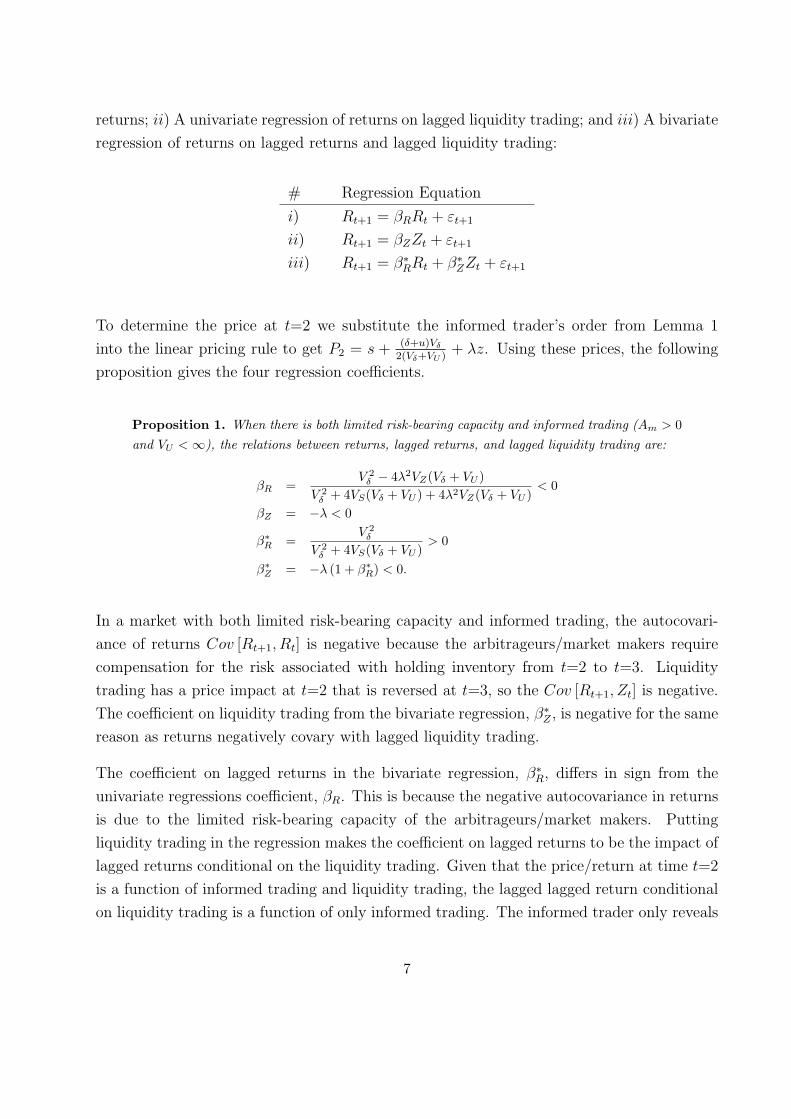
returns; ii) A univariate regression of returns on lagged liquidity trading; and iii) A bivariate
regression of returns on lagged returns and lagged liquidity trading:
# Regression Equation
i) Rt+1 = βRRt + εt+1
ii) Rt+1 = βZZt + εt+1
iii) Rt+1 = β∗RRt + β∗ZZt + εt+1
To determine the price at t=2 we substitute the informed trader’s order from Lemma 1
into the linear pricing rule to get P2 = s + (δ+u)Vδ2(Vδ+VU )
+ λz. Using these prices, the following
proposition gives the four regression coefficients.
Proposition 1. When there is both limited risk-bearing capacity and informed trading (Am > 0and VU <∞), the relations between returns, lagged returns, and lagged liquidity trading are:
βR =V 2δ − 4λ2VZ(Vδ + VU )
V 2δ + 4VS(Vδ + VU ) + 4λ2VZ(Vδ + VU )
< 0
βZ = −λ < 0
β∗R =V 2δ
V 2δ + 4VS(Vδ + VU )
> 0
β∗Z = −λ (1 + β∗R) < 0.
In a market with both limited risk-bearing capacity and informed trading, the autocovari-
ance of returns Cov [Rt+1, Rt] is negative because the arbitrageurs/market makers require
compensation for the risk associated with holding inventory from t=2 to t=3. Liquidity
trading has a price impact at t=2 that is reversed at t=3, so the Cov [Rt+1, Zt] is negative.
The coefficient on liquidity trading from the bivariate regression, β∗Z , is negative for the same
reason as returns negatively covary with lagged liquidity trading.
The coefficient on lagged returns in the bivariate regression, β∗R, differs in sign from the
univariate regressions coefficient, βR. This is because the negative autocovariance in returns
is due to the limited risk-bearing capacity of the arbitrageurs/market makers. Putting
liquidity trading in the regression makes the coefficient on lagged returns to be the impact of
lagged returns conditional on the liquidity trading. Given that the price/return at time t=2
is a function of informed trading and liquidity trading, the lagged lagged return conditional
on liquidity trading is a function of only informed trading. The informed trader only reveals
7

part of his information via trading, so the return at t=3 is positively correlated with the
informed trading at t=2.
To formulate how limited risk-bearing capacity and the presence of informed trading sepa-
rately affect the regression coefficients, we study two cases: i) Unlimited risk-bearing capac-
ity and informed trading; and ii) Limited risk-bearing capacity with no informed trading.
The following two corollaries provide the regression coefficients for these two cases. Note
that the case of both unlimited risk-bearing capacity and no informed trading makes trivial
predictions. Prices only change due to public signals and all regression coefficients are zero.
Corollary 1. When there is unlimited risk-bearing capacity, Am = 0, the price impact func-tion has the closed-form solution: λ = Vδ
2√VZ(Vδ+VU )
. The univariate and bivariate regression
coefficients of returns on lagged returns and lagged liquidity trading are:
βR = 0
βZ = − Vδ
2√VZ(Vδ + VU )
< 0
β∗R =V 2δ
V 2δ + 4VS(Vδ + VU )
> 0
β∗Z = − Vδ (1 + β∗R)2√VZ(Vδ + VU )
< 0
When the arbitrageurs are risk averse, stock returns are negatively autocorrelated (βR < 0
in Regression i). In the case of Corollary 1, arbitrageurs are risk neutral (Am = 0) and prices
are a martingale ((βR = 0 in Regression i).
Corollary 2. When the informed trader’s private signal consists entirely of noise, VU=∞,there is no informed trading and the price impact function has the closed-form solution: λ =12AmVδ. The univariate and bivariate regression coefficients of returns on lagged returns andlagged liquidity trading are:
βR = − A2mV
2δ VZ
4VS +A2mV
2δ VZ
< 0
βZ = −12AmVδ < 0
β∗R = 0
β∗Z = −12AmVδ < 0
When there is no informed trading, the arbitrageurs need not worry about adverse selection.
Price changes due to order imbalances arise solely from liquidity trading and are fully re-
8

versed. Lagged returns conditional on lagged liquidity trading no longer provide information
about informed trading, so β∗R=0.
[ Insert Table 1 About Here ]
Table 1 summarizes the model’s predictions. Comparing across rows and columns illus-
trates how the model’s predictions differ depending on the two frictions: limited risk-bearing
capacity and adverse selection.
3 Data
Our data span seven years (1,756 trading days) from January 1999 to December 2005. We
obtain the data from a number of sources. The Center for Research in Security Prices
(CRSP) provides daily prices, share volumes, and shares outstanding for all common stocks
listed on the New York Stock Exchange (NYSE). We calculate daily midquote stock returns
using the NYSE’s Trades and Quotes (TAQ) database and the closing bid/ask quotes. The
TAQ Master file allows us to match stock symbols with CUSIP numbers which are then
matched with the NCUSIP field in the CRSP data. The use of midquote returns eliminates
issues of bid-ask bounce that are present in transaction-based (CRSP) returns.
[ Insert Table 2 About Here ]
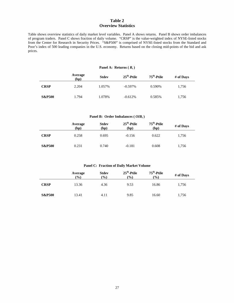
Table 2, Panel A shows overview statistics for the return data. Throughout the paper, we
define “the market” using two groupings. The the first contains all CRSP-NYSE stocks.
The second contains all S&P500-NYSE stocks. Untabulated results show our data contain
an average of 1,557 CRSP-NYSE stocks per day and 413 S&P500-NYSE common stocks per
day.
The full sample of CRSP-NYSE stocks has a slightly higher average return (2.204 basis
points per day) than the S&P500-NYSE stocks (1.794 basis points per day). Otherwise,
returns from the two market aggregations appear similar. Finally, and also not tabulated,
the index of CRSP-NYSE stocks based on daily midquote returns has a 0.944 correlation
with the index based on closing-price returns.
9

3.1 Order Imbalance Data
Our order imbalance data come from the NYSE’s Consolidated Equity Audit Trail (CAUD)
dataset. The data contain information about all executed NYSE trades including transac-
tion: price, number of shares, amount, buyer account type, and seller account type. We
focus on the Program Trader (“PT”) account type. As discussed in the next paragraph, the
NYSE’s definition for PT makes it natural to think of these trades as portfolio trades. To
minimize the influence of index arbitrage activity, we exclude data from the account type
“Program Index Arbitrages Traders”. A stock’s order imbalance (OIB i,t) is defined as dollars
bought minus dollars sold all divided by the market capitalization.
The NYSE defines program trading as the purchase or sale of 15 or more stocks having a
total market value of $1 million or more. With increased automation and the end of fixed
commissions, brokers began offering the ability to execute program trades at very low cost.
PT was closely studied after the 1987 market disruptions. Investors following strategies
related to portfolio insurance sold S&P500 futures as stock prices fell. This price pressure
made futures cheaper than the underlying equities. Index arbitragers, who accounted for
roughly a third of program trades at that time, transmitted this price pressure to the un-
derlying stocks. The magnitude of this price pressure piqued the interest of regulators and
academics in the links between intraday price discovery, volatility in the futures market, and
volatility in the equity market—see Greenwald and Stein (1988). Initial program trading
studies focus on the relationship between program trading, volatility, and futures prices—see
Harris, Sofianos, and Shapiro (1994) and Hasbrouck (1996). In contrast, our data is designed
to filter out the index arbitrage component of program trading and we examine PT’s impact
at interday horizons.
Since 1987 program trading by index traders has increased as the value of exchange-traded
funds and index-linked derivatives has grown by hundreds of billions and trillions of dollars.
Contracts based on the S&P500 Index are the most heavily traded (ETFs, futures, and
options). The advantages of program trading for index traders are its efficiency and low
costs.7 Program trades may be low cost because those trading a basket of securities can signal
they have little or no information about the underlying stocks—Subrahmanyam (1991a).
Table 1, Panel B shows that program traders have been accumulating shares over the sample
7Bloomberg, “Program Trades Dominate NYSE 18 Years After Crash: Taking Stock,” October 19, 2005, quotesthe head of equity trading at the biggest manager of ETFs, Barclays Global Investors, as using program tradingbecause “it increases efficiency and reduces costs.”
10

period. The average daily value is 0.258 basis points per day for the CRSP-NYSE stocks with
a 0.695 standard deviation. Again, we see similar variables with the S&P500-NYSE stocks.
Figure 1 graphs our market-wide OIB measure in units of fraction of market capitalization.
Panel A shows the measure for the sample of CRSP-NYSE stocks. Panel B shows the
measure for the S&P500-NYSE stocks.
[ Insert Figure 1 About Here ]
During our sample period the total market capitalization of NYSE S&P500 stocks is roughly
$8 trillion, making the 0.740 basis point standard deviation of OIB correspond to about
$600 million. Days with imbalances that exceed three basis points of aggregate S&P500
capitalization correspond to order imbalances of approximately $2.5 billion. The volatility
of OIB t appears somewhat higher at the beginning of the sample compared with the end of
the sample.
As an additional test of program traders contemporaneously buying and selling across stocks
in the market index, we conduct a principal component analysis. Calculating principal
components requires that the time series be larger than the cross section, so as in Hasbrouck
and Seppi (2001) we focus on the 28 NYSE-listed stocks in the Dow Jones Industrial Index.
The first four principal components explain 15.15%, 5.54%, 4.87%, and 4.34% of daily OIB i,t
correlation. The first component is both economically and statistically significant indicating
program traders tend to buy and sell stocks in the index at the same time.
Table 2, Panel C shows the program traders’ fraction of daily market volume. The trading
volume of program traders equals the dollar value of their buys plus sells. The program
traders account for an average of 13.36% of market volume. This fraction is similar when
looking only at S&P500 stocks.8
3.2 Correlations of Returns and OIB
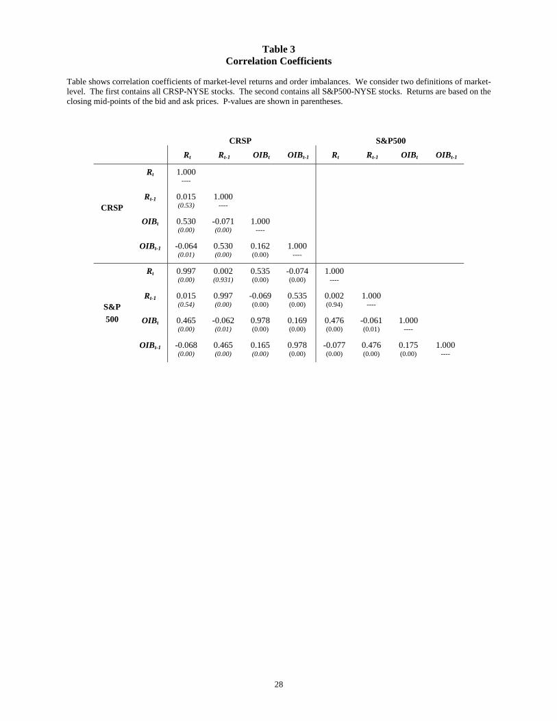
Table 3 reports the correlation of value-weighted market returns and order imbalances for
all CRSP-NYSE stocks as well as only the S&P500-NYSE stocks. The table also includes
8When the NYSE reports program trading as a percentage it typically reports program trading buys plus sellsdivided by total volume. If all trades were program trades, the NYSE would report that 200% of trading volumewas due to program trading. Therefore, we calculate total volume as buy volume plus sell volume, which is twicethe trading volume reported in TAQ or CRSP. Our approach leads to our program trading percentages being half aslarge as those reported by the NYSE.
11
lagged returns and lagged order imbalances.
[ Insert Table 3 About Here ]
When looking at CRSP-NYSE stocks, returns are not autocorrelated. The AR(1) coefficient
is 0.015 with a 0.53 p-value. On the other hand, OIB t has a positive AR(1) coefficient
of 0.162 with a 0.00 p-value. The contemporaneous correlation between Rt and OIB t is
0.530 and significant at all conventional levels. This indicates that PTs contemporaneously
move prices or PTs engage in high-frequency (intraday) positive feedback trading. OIB is
contrarian at a one-day lag with a -0.071 correlation between OIB t and Rt−1. Similar results
hold for the S&P500-NYSE stocks
Most intriguingly, OIB t negatively predicts market returns one day ahead as seen by the
-0.064 correlation between OIB t−1 and Rt. Some evidence of related effects is found in
Chordia, Roll, and Subrahmanyam (2002). Their measure of OIB t constructed using a
trade-signing algorithm does not predict market returns in their entire sample, but does
predict S&P500 returns the following day when OIB t and returns are both very negative on
the same day.
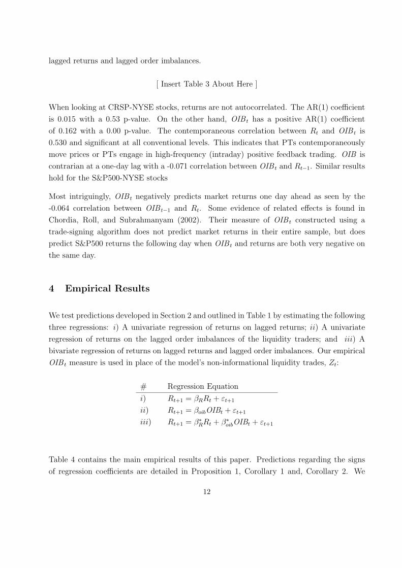
4 Empirical Results
We test predictions developed in Section 2 and outlined in Table 1 by estimating the following
three regressions: i) A univariate regression of returns on lagged returns; ii) A univariate
regression of returns on the lagged order imbalances of the liquidity traders; and iii) A
bivariate regression of returns on lagged returns and lagged order imbalances. Our empirical
OIB t measure is used in place of the model’s non-informational liquidity trades, Zt:
# Regression Equation
i) Rt+1 = βRRt + εt+1
ii) Rt+1 = βoibOIBt + εt+1
iii) Rt+1 = β∗RRt + β∗oibOIBt + εt+1
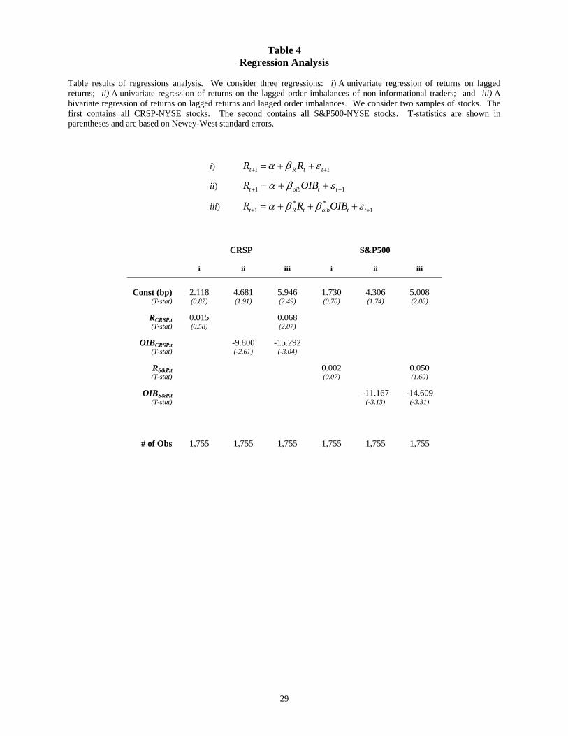
Table 4 contains the main empirical results of this paper. Predictions regarding the signs
of regression coefficients are detailed in Proposition 1, Corollary 1 and, Corollary 2. We
12
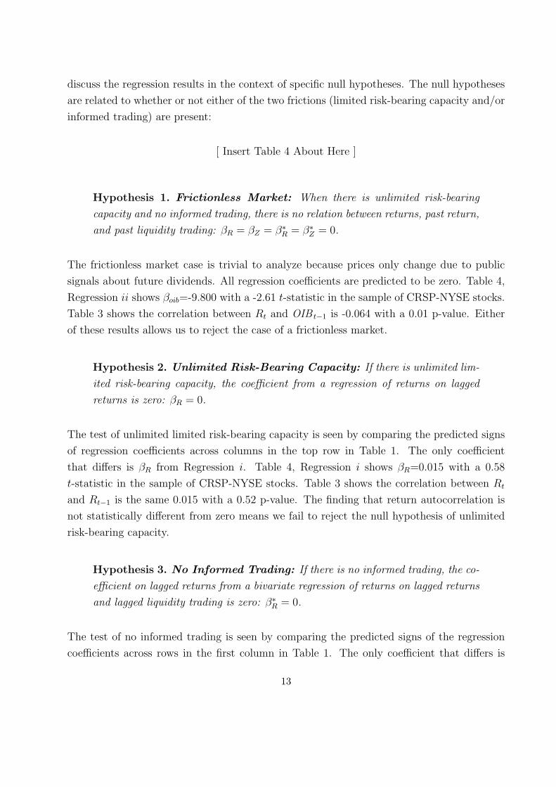
discuss the regression results in the context of specific null hypotheses. The null hypotheses
are related to whether or not either of the two frictions (limited risk-bearing capacity and/or
informed trading) are present:
[ Insert Table 4 About Here ]
Hypothesis 1. Frictionless Market: When there is unlimited risk-bearing
capacity and no informed trading, there is no relation between returns, past return,
and past liquidity trading: βR = βZ = β∗R = β∗Z = 0.
The frictionless market case is trivial to analyze because prices only change due to public
signals about future dividends. All regression coefficients are predicted to be zero. Table 4,
Regression ii shows βoib=-9.800 with a -2.61 t-statistic in the sample of CRSP-NYSE stocks.
Table 3 shows the correlation between Rt and OIB t−1 is -0.064 with a 0.01 p-value. Either
of these results allows us to reject the case of a frictionless market.
Hypothesis 2. Unlimited Risk-Bearing Capacity: If there is unlimited lim-
ited risk-bearing capacity, the coefficient from a regression of returns on lagged
returns is zero: βR = 0.
The test of unlimited limited risk-bearing capacity is seen by comparing the predicted signs
of regression coefficients across columns in the top row in Table 1. The only coefficient
that differs is βR from Regression i. Table 4, Regression i shows βR=0.015 with a 0.58
t-statistic in the sample of CRSP-NYSE stocks. Table 3 shows the correlation between Rt
and Rt−1 is the same 0.015 with a 0.52 p-value. The finding that return autocorrelation is
not statistically different from zero means we fail to reject the null hypothesis of unlimited
risk-bearing capacity.
Hypothesis 3. No Informed Trading: If there is no informed trading, the co-
efficient on lagged returns from a bivariate regression of returns on lagged returns
and lagged liquidity trading is zero: β∗R = 0.
The test of no informed trading is seen by comparing the predicted signs of the regression
coefficients across rows in the first column in Table 1. The only coefficient that differs is
13

the bivariate regression coefficient β∗R. Using CRSP-NYSE stocks, Table 4, Regression iii
estimates β∗R=0.068 with a 2.07 t-statistic. The positive coefficient on returns, β∗R, allows us
to reject the null hypothesis of no informed trading.
Using the CRSP-NYSE stocks, the coefficients in Table 4 Regressions i, ii, and iii are
βR=0.015 with a 0.58 t-statistic; βoib=-9.800 with a -2.61 t-statistic; β∗R=0.068 with a 2.07
t-statistic; and β∗oib=-15.292 with a -3.01 t-statistic. The signs of these regressions coefficients
fit the predictions of Corollary 1: βR =0, βoib <0, β∗R >0, and β∗oib <0. We repeat the three
regressions using S&P500-NYSE stocks and find similar results except that β∗R is positive at
the 11%-level.
Overall, our findings are consistent with the theoretical predictions based on the unlimited
risk-bearing capacity and informed trading case in the upper right quadrant of Table 1
(Corollary 1). Put differently, we find evidence to support there being informed trading at
the market level, but do not find evidence to support limited risk-bearing capacity at the
market level.
4.1 Vector Autoregression Results
Table 3 shows order imbalances are positively autocorrelated and negatively correlated with
lagged returns. To control for these effects, we estimate a vector autoregression using returns
and OIB t. In Equation 2, each of the Φk matrices is dimension two-by-two and has four
coefficients to be estimated. The errors are distributed: εt ∼ N[0,Ω]. The HQIC criteria
indicates we should include four lags such that K=4 and k=1, 2, 3, 4.
Yt = c+ Φ1Yt−1 + Φ2Yt−2 + Φ3Yt−3 + Φ4Yt−4 + εt (2)
Yt =
[OIBtRt
]c =
[αoib
αr
]Φk =
[φk,1,1 φk,1,2
φk,2,1 φk,2,2
]εt =
[εoibt
εrt
]
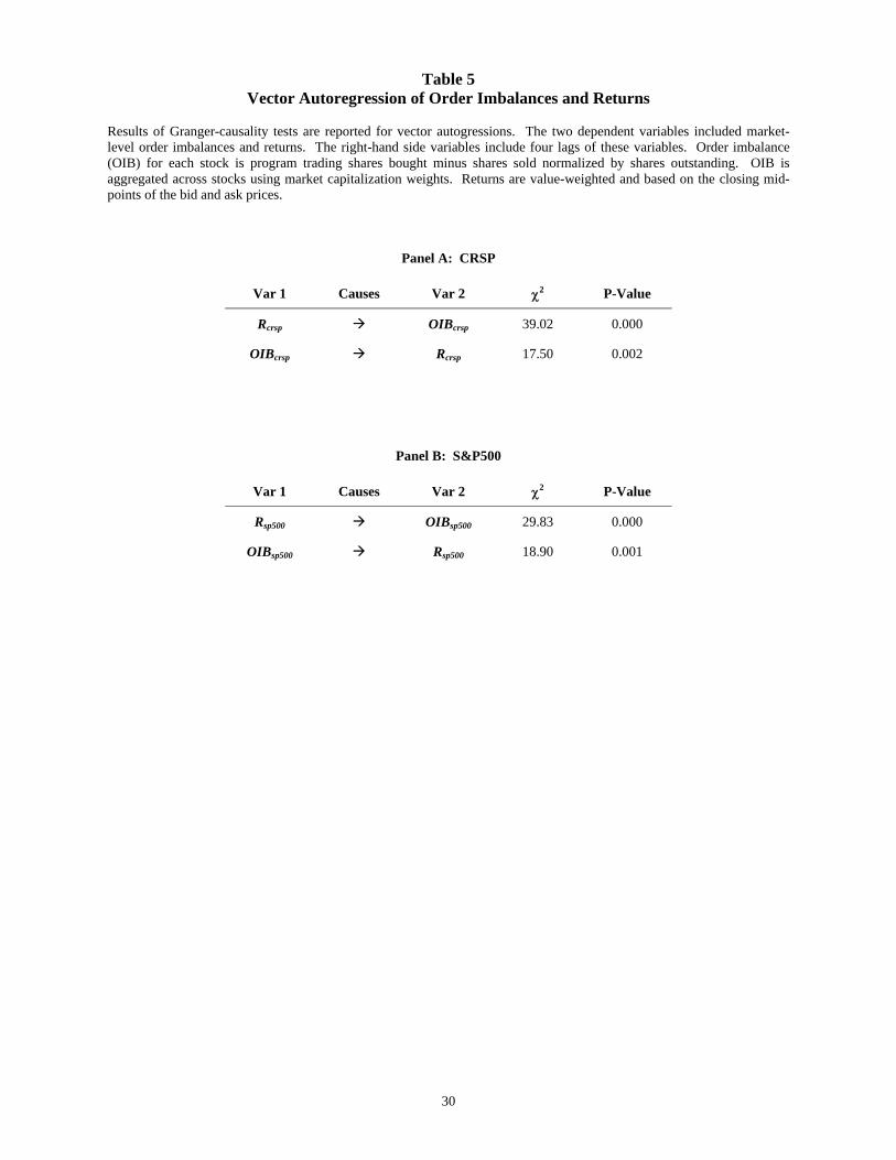
Table 5 reports Granger causality results. We show there exists bidirectional causality be-
tween returns and OIB. Most importantly, we show OIB t Granger causes returns. The
relationship is significant at all conventional levels as the 39.02 χ2 statistic shows. This
along with the coefficients on lagged OIB t shows the predictability of market returns. Also,
we see that returns Granger cause OIB t at all conventional levels of significance due to the
negative feedback trading behavior by the program traders.
14
[ Insert Table 5 About Here ]
A parsimonious way of capturing the net effects of all the coefficients in the VAR is to follow
Hamilton (1994) and form orthogonalized impulse response functions (IRFs). The unit-shock
IRF at horizon t+s is denoted Φs and comes from recursively solving the following: Ψ1 = Φ1
and Ψs = Φ1Ψs−1 + Φ2Ψs−2 + . . . + ΦPΨs−K . The orthogonalized shock is obtained by
factoring the covariance matrix of the error term Ω = PP′ where P is lower diagonal. Denote
the jth column of P as Pj. The IRF, or change to Yt+s in response to an orthogonalized
shock at t=0, is given by ΨsPj.
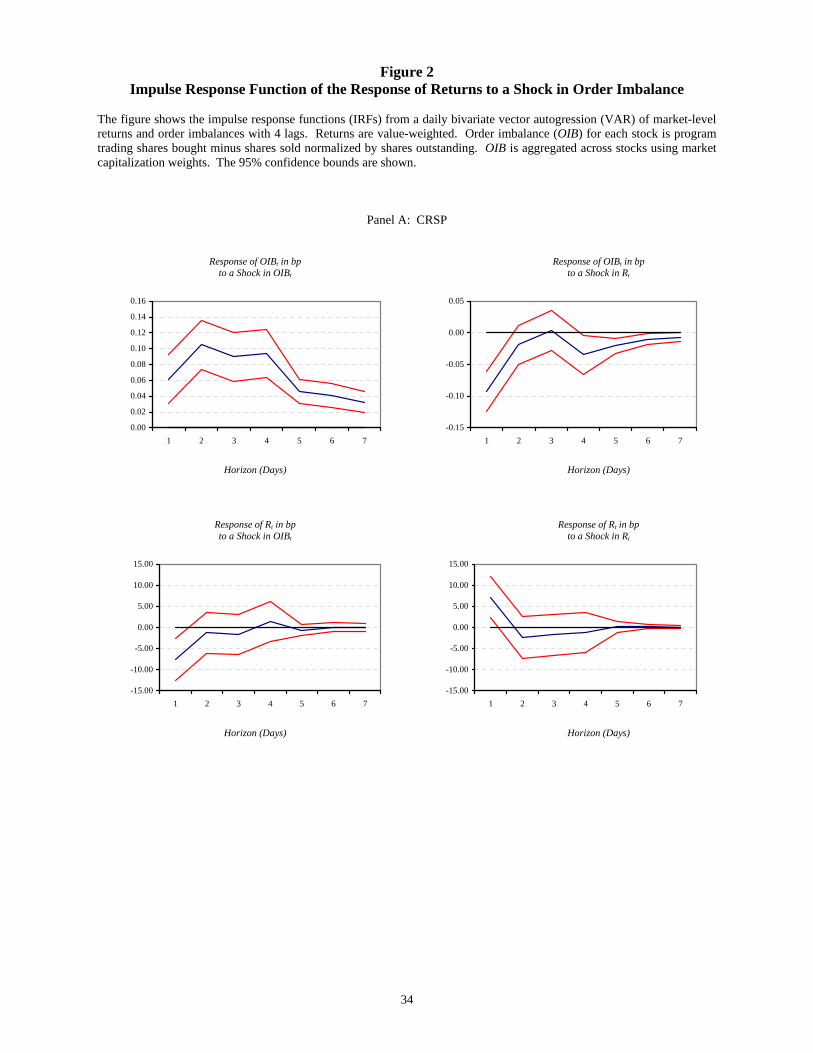
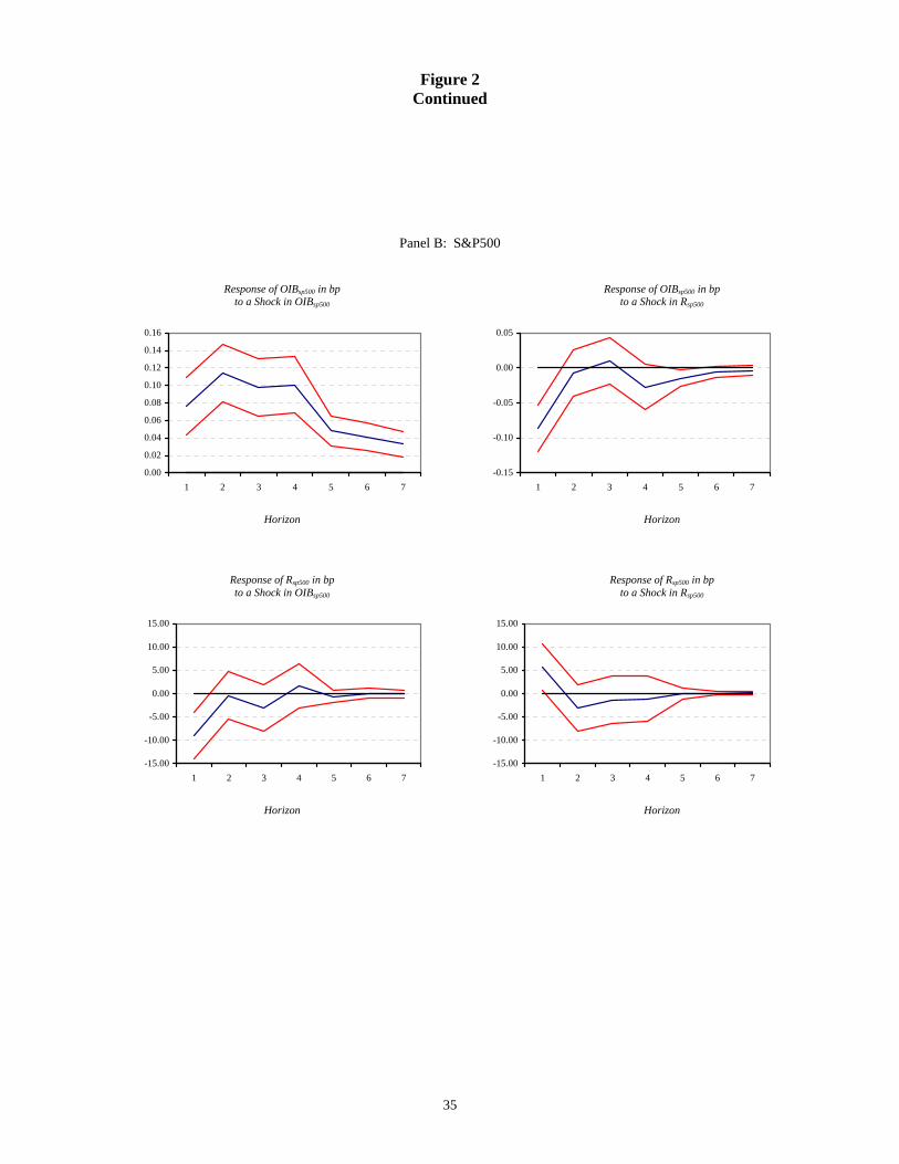
Figure 2, Panel A has four sub-panels. The focus of this paper is the lower-left panel. We
see that a one standard deviation shock to OIB t leads to a -7.52 bp return the following
day. The effect is short-lived and not significant after one day. The VAR results in Figure 2
show that the regression results in Table 4 are robust to a more general specification that
controls for the autocorrelation in order imbalances and the negative correlation between
order imbalances and lagged returns.
[ Insert Figure 2 About Here ]
Figure 2 shows the positive autocorrelation of OIB t in the top-left panel. The top-right
panel gives evidence of the negative feedback trading. A one standard deviation shock to
returns causes a 0.09 bp decrease in OIB t. Figure 2, Panel B shows similar impulse response
functions for the sample of S&P500-NYSE stocks. The conditional autocorrelation is shown
in the lower-right graph. We see that the ability of past return shocks to predict one-day
ahead returns is positive and significant at the 5%-level.
5 Are Program Traders Uninformed?
We calculate the returns and revenues associated with our portfolio trading imbalances. If
OIB t represents non-informational order imbalances, we expect the trades to lose money.
To calculate the returns associated with OIB t, we follow standard calendar-time portfolio
methodology and create separate “buy” and “sell” portfolios. For this paper, we assume a
two day holding period which consists of the intra-day return on t=0, the return on t+1 and
the return on t+2.
15
We begin by calculating the value-weighted average buying price for program traders in
aggregate, for each stock i, on each date t=0. The value-weighted price (VWAP buyi,t=0) is the
dollar value of all shares bought by PT divided by number of shares bought by PT. The
intra-day return on date t=0 is calculated using the closing midquote of bid and ask prices:
1 + Rbuyi,t=0 = Closemidqi,t=0/VWAP buy
i,t=0. To calculate holding period returns on date t+1 and
t+2 we using midquote to midquote returns. Similar expressions hold for stocks sold.
The calendar-time buy portfolio return is the value weighted return of stocks in the portfolio
on a given day. Value-weighting is determined by the number of shares originally bought by
the program traders and the value of these shares. The value of the shares may change with
market conditions but the number of shares does not.
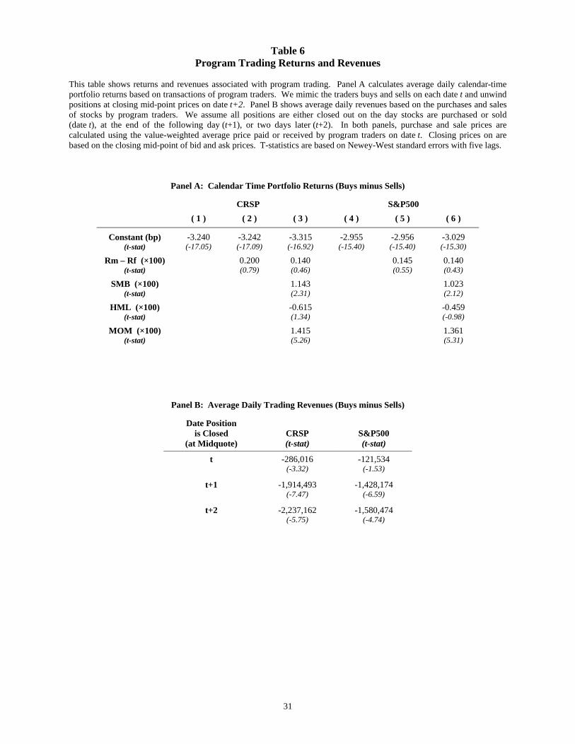
Table 6, Panel A regresses the returns of the value-weighted Buy minus Sell portfolio on a
constant, the market’s excess returns, the Fama-French factors, and the Carhart momentum
factor. We report results for both CRSP-NYSE stocks and for S&P500-NYSE stocks. The
“alpha” or constant in the regression is both econmically and statistically less than zero. For
example, and alpha of -3 basis points (bp) corresponds to a loss of 7.85% per annum. The
reported t-statistics are in the -15 range indicating significance at all conventional levels.
[ Insert Table 6 About Here ]
We also calculate the daily dollar revenues associated with OIB trades. To calculate revenues
we again focus on the amount bought and sold, of each stock, on each day. From the calendar-
time portfolios (above) we know the difference between the value-weighted average buying
price and the closing midquote price. For example, the revenues associated with buying or
selling a given stock on date t and closing out the position on date t+2 are given by:9
Revbuyi,t+2 = Amount($)buyi,t=0 ×[(
1 +Rbuyi,t=0
)·(
1 +Rmidqi,t+1
)·(
1 +Rmidqi,t+2
)− 1]
Revselli,t+2 = Amount($)selli,t=0 ×[(
1 +Rselli,t=0
)·(
1 +Rmidqi,t+1
)·(
1 +Rmidqi,t+2
)− 1]
(3)
Revi,t+2 = Revbuyi,t+2 −Revselli,t+2
We sum revenues across stocks on the same day to form a single time series of revenues.
9This calculation is equivalent to how generally accepted accounting principles have financial firms calculate grosstrading revenues where open positions are marked to a market value (in our case the closing quote midpoint).
16
Results are shown in Table 7, Panel B.
On date t, program traders buy slightly above the closing midquote and sell slightly below
the same value (on average). The results show an average daily revenue of $-286,016 with
a -3.32 t-statistic. Therefore, there is no evidence that program traders make money at
intraday horizons.
Consistent with program trading negatively predicting future market returns, if stocks are
held an additional day or two, mark-to-market losses increase significantly. The average
daily revenue is $-1,914,493 with a -7.47 t-statistic if positions are closed out at the end of
date t+1. The average daily revenue is $-2,237,162 if positions are closed out on date t+2.
Table 7 reports t-statistics based on Newey-West standard errors with five lags. Similar
results hold for the sample of S&P500-NYSE stocks. The results in this section show that
program traders lose money, so it is natural to think of program trading as non-informational.
6 Index Additions
Studies of additions to the the S&P500 Index often cite non-informational traders who trade
all stocks in the S&P500 Index as the explanation for their results. Program trading is by
definition trading in a large basket of stocks and the prior section establishes that program
trading is non-informational liquidity trading. Therefore, program trading order imbalances
provide a natural way to examine if there is a relationship between non-informational traders
and results from studies of changes to the S&P500 Index.
To examine whether program trading changes after a stock joins the S&P500 Index we con-
struct a sample of 90 NYSE-listed additions starting in January 2000 and ending December
2004 (skipping a year at the beginning and end of the same in order to estimate the comove-
ment results described below). Of these, the year 2000 has the most additions (31), while
the year 2003 has the fewest (5). Our events occur on 57 different days. Four days have two
additions, one day has four additions, and one day has five additions.
In results not tabulated we compare our additions to existing event studies. In our sample,
prices jump up 4% on average on the announcement date and then hold steady. This increase
is comparable to Chen, Noronha, and Singal (2004) for their 1989 to 2000 sample period.
Consistent with Hegde and McDermott (2003), we measure an increase in turnover and
decline in spreads around additions. Both are statistically significant. Finally we measure
17
an increase in return comovement that similar to results in Vijh (1994) and Barberis, Shleifer,
and Wurgler (2005).
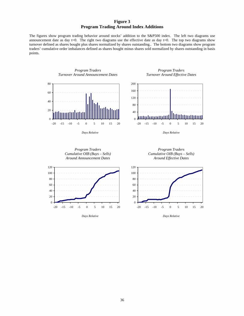
[ Insert Figure 3 About Here ]
The above papers on S&P additions posit that their results are due to a group of traders who
trade all stocks in the S&P500 Index. To link our order imbalance measure to index additions
we first calculate the average level of daily program trading during the t = [−20,+20] event
window. Figure 3 highlights the difference between aligning events by announcement dates
and by effective dates.10 The upper-right graph shows that program traders experience a
sharp increase in turnover on the last day before a stock joins the index. The lower right
graph shows that the increased turnover is due (partially) to program traders accumulating
shares of the added stock. Between t = −20 and t = +20, the program traders acquire
approximate 1.1% of the company’s shares. Table 7, Panel A provides the some of the
numbers behind the Figure 3.
[ Insert Table 7 About Here ]
Vijh (1994) and Barberis, Shleifer, and Wurgler (2005) cite non-informational traders focus-
ing on the S&P500 stocks as being the source of the changes in comovement upon addition
to the index. To test this we first measure the change in OIB i,t comovement from the
[−250,−51] interval to the [+51,+250] interval. We start with a univariate regression to
quantify changes in comovement. Regression (4) is performed separately for each of the
event stocks both before and after the addition. We record the βoibsp500,i and R2 for each
regression before comparing pre- and post-event values. For all comovement regressions,
OIB sp500,t is the market-capitalization weighted average of OIB i,t across all S&P500-NYSE
stocks not including stock i.
OIBi,t = αi + βoibsp500,i (OIBsp500,t) + εi,t. (4)
Table 7, Panel B show that both R2 and βoibsp500 increase after a stock is added to the S&P500
Index. These increases are both statistically significant with 4.03 and 3.86 t-statistics re-
spectively. Both the βoibsp500 and the R2 show near three-fold increases post addition.
10The last date before a stock joins the index is called the “effective date” and is available from Standard andPoor’s website. Each event’s “announcement date” is originally obtained from Jeffrey Wurgler’s website and thenmodified by searching news releases. The average difference between the two dates is 7.03 trading days. The standarddeviation of the difference is 6.79 days.
18
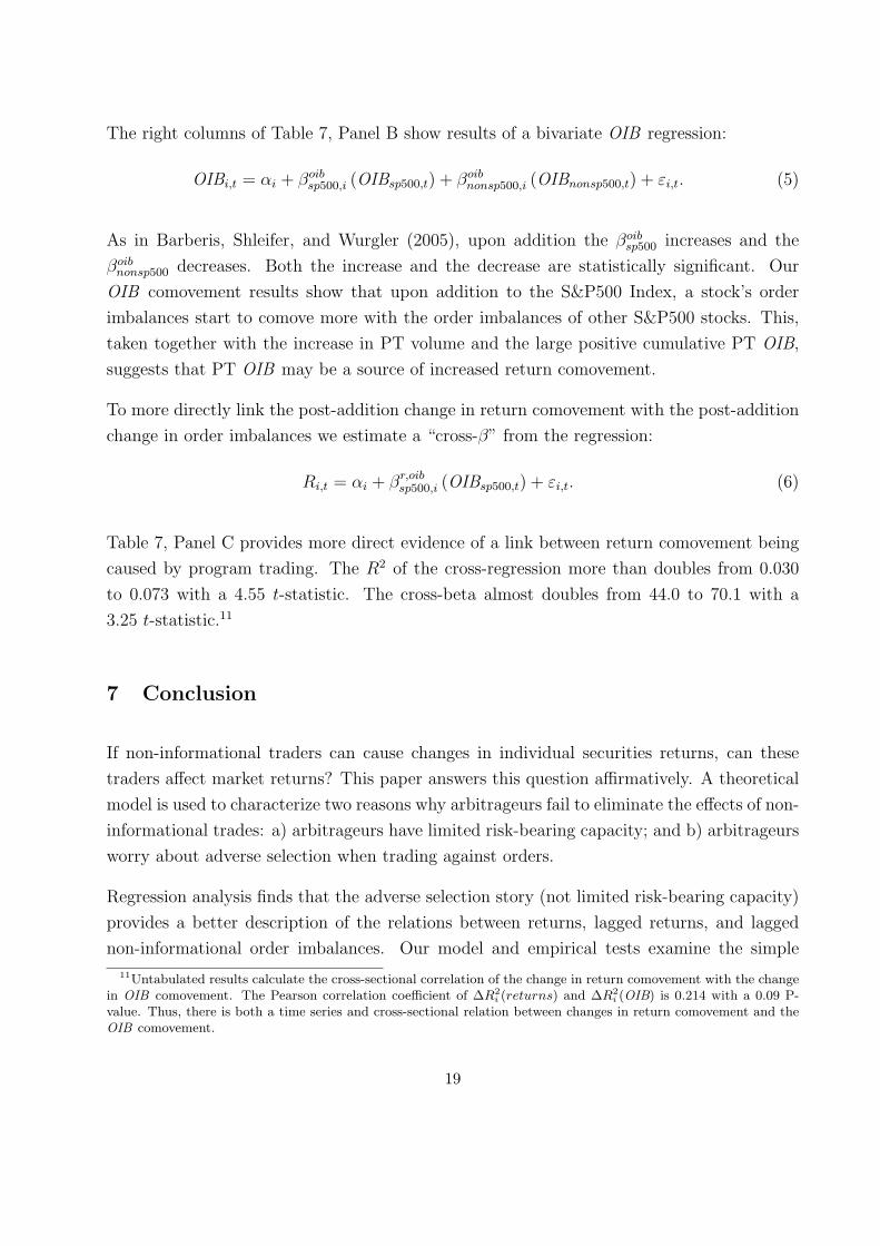
The right columns of Table 7, Panel B show results of a bivariate OIB regression:
OIBi,t = αi + βoibsp500,i (OIBsp500,t) + βoibnonsp500,i (OIBnonsp500,t) + εi,t. (5)
As in Barberis, Shleifer, and Wurgler (2005), upon addition the βoibsp500 increases and the
βoibnonsp500 decreases. Both the increase and the decrease are statistically significant. Our
OIB comovement results show that upon addition to the S&P500 Index, a stock’s order
imbalances start to comove more with the order imbalances of other S&P500 stocks. This,
taken together with the increase in PT volume and the large positive cumulative PT OIB,
suggests that PT OIB may be a source of increased return comovement.
To more directly link the post-addition change in return comovement with the post-addition
change in order imbalances we estimate a “cross-β” from the regression:
Ri,t = αi + βr,oibsp500,i (OIBsp500,t) + εi,t. (6)
Table 7, Panel C provides more direct evidence of a link between return comovement being
caused by program trading. The R2 of the cross-regression more than doubles from 0.030
to 0.073 with a 4.55 t-statistic. The cross-beta almost doubles from 44.0 to 70.1 with a
3.25 t-statistic.11
7 Conclusion
If non-informational traders can cause changes in individual securities returns, can these
traders affect market returns? This paper answers this question affirmatively. A theoretical
model is used to characterize two reasons why arbitrageurs fail to eliminate the effects of non-
informational trades: a) arbitrageurs have limited risk-bearing capacity; and b) arbitrageurs
worry about adverse selection when trading against orders.
Regression analysis finds that the adverse selection story (not limited risk-bearing capacity)
provides a better description of the relations between returns, lagged returns, and lagged
non-informational order imbalances. Our model and empirical tests examine the simple
11Untabulated results calculate the cross-sectional correlation of the change in return comovement with the changein OIB comovement. The Pearson correlation coefficient of ∆R2
i (returns) and ∆R2i (OIB) is 0.214 with a 0.09 P-
value. Thus, there is both a time series and cross-sectional relation between changes in return comovement and theOIB comovement.
19

market-wide arbitrage strategy of market-wide liquidity provision. The lack of evidence
for limited risk-bearing capacity for this strategy suggests that specialization is empirically
important for the Shleifer and Vishny (1997) limits to arbitrage arguments.12
12At least during our sample period in U.S. markets. It is interesting to note that that there is evidence of limitedrisk-bearing capacity beginning with the recent financial crisis: the autocorrelation of daily returns on the S&P500Index becomes significantly negative, close to -0.15 in both 2007 and 2008. This recent evidence on limit-risk bearingcapacity suggests less capital being devoted to market liquidity provision, possibly due to wealth affects.
20

References
[1] Admati, Anat, and Paul Pfleiderer, 1988, A theory of intraday patterns: volume and
price variability, Review of Financial Studies 1, 3-40.
[2] Amihud, Yakov, and Haim Mendelson, 1980, Dealership market: Market making with
inventory, Journal of Financial Economics 8, 31-54.
[3] Andrade, Sandro, Charles Chang, and Mark Seasholes, 2008, Trading imbalances, pre-
dictable reversals, and cross-stock price pressure, Journal of Financial Economics, 88(2)
May, 406-423.
[4] Bessembinder, Hendrik, 2003, Issues in assessing trade execution costs, Journal of Fi-
nancial Markets, Journal of Financial Markets 6, 233-257.
[5] Boehmer, Ekkehart, and Julie Wu, 2008, Order flow and prices, working paper.
[6] Chan, Kalok, Allaudeen Hameed, and Sie Lau, 2003, What if trading location is different
from business location? Evidence from the Jardine Group, Journal of Finance 58, 1221-
1246.
[7] Chen, Honghui, Gregory Noronha, and Vijay Singal, 2004, The price response to S&P
500 index additions and deletions: Evidence of Asymmetry and a new explanation,
Journal of Finance 59, 1901-1929.
[8] Chordia, Tarun, Richard Roll, and Avanidhar Subrahmanyam, 2002, Order imbalance,
liquidity and market returns, Journal of Financial Economics 65, 111-130.
[9] Chordia, Tarun, Richard Roll, and Avanidhar Subrahmanyam, 2008, Liquidity and
market efficiency, Journal of Financial Economics 87, 249-268.
[10] Chordia, Tarun, and Avanidhar Subrahmanyam, 2004, Order imbalances and individual
stock returns: theory and evidence, Journal of Financial Economics 72, 485-518.
[11] Coval, Joshua, and Erik Stafford, 2007, Asset fire sales (and purchases) in equity mar-
kets, Journal of Financial Economics 86, 479-512.
[12] Evans, Martin, and Richard Lyons, 2002, Order flow and exchange rate dynamics,
Journal of Political Economy, 110, 170-180.
[13] Evans, Martin, and Richard Lyons, 2005, A new micro model of exchange rate dynamics,
Working paper.
21
[14] Evans, Martin, and Richard Lyons, 2008, Forecasting exchange rates and fundamentals
with order flow, Working paper.
[15] Froot, Kenneth and Emil Dabora, 1999, How are stock prices affected by the location
of trade? Journal of Financial Economics 53, 189-216.
[16] Greenwald, Bruce and Jeremy Stein, 1988, The task force report: The reasoning behind
the recommendations, Journal of Economic Perspectives 2, 3-23.
[17] Greenwood, Robin, 2005, Short- and long-term demand curves for stocks: Theory and
evidence on the dynamics of arbitrage, Review of Financial Studies 75, 607-649.
[18] Greenwood, Robin, 2008, Excess comovement of stock returns: Evidence from cross-
sectional variation in Nikkei 225 weights, Review of Financial Studies 21, 1153-1186.
[19] Grossman, Sanford, and Merton Miller, 1988, Liquidity and market structure, Journal
of Finance 43, 617-633.
[20] Hamilton, James D., 1994, Time series analysis, Princeton University Press.
[21] Harris, Lawrence, George Sofianos, and James Shapiro, 1994, Program trading and
intraday volatility, Review of Financial Studies 7, 653-685.
[22] Hasbrouck, Joel, 1996, Order characteristics and stock price evolution: an application
to program trading, Journal of Financial Economics 41, 129-149.
[23] Hasbrouck, Joel, and Duane Seppi, 2001, Common factors in prices, order flows, and
liquidity, Journal of Financial Economics 59, 383-411.
[24] Hegde, Shantaram, and John McDermott, 2003, The liquidity effect of revisions to the
S&P 500 index: an empirical analysis, Journal of Financial Markets 6, 413-459.
[25] Hendershott, Terrence, and Mark Seasholes, 2007, Market maker inventories and stock
prices, American Economic Review 97, 210-214.
[26] Ho, Thomas, and Hans Stoll, 1981, Optimal dealer pricing under transactions and return
uncertainty, Journal of Financial Economics 9, 47-73.
[27] Kaniel, Ron, Gideon Saar, and Sheridan Titman, 2008, Individual investor trading and
stock returns Journal of Finance 63, 273-310.
[28] Kyle, Albert, 1985, Continuous auctions and insider trading, Econometrica 53, 1315-
1335.
22

[29] Madhavan, Ananth, and Seymour Smidt, 1993, An analysis of daily changes in specialist
inventories and quotations, Journal of Finance 48, 1595-1628.
[30] Pirinsky, Christo, and Qinghai Wang, 2006, Does corporate headquarters location mat-
ter for stock returns? Journal of Finance 61, 1991-2015.
[31] Shleifer, Andrei, and Robert Vishny, 1997, The limit of arbitrage, Journal of Finance
52, 35-55.
[32] Subrahmanyam, Avanidhar, 1991a, A theory of trading in stock index futures, Review
of Financial Studies 4(1), 17-51.
[33] Subrahmanyam, Avanidhar, 1991b, Risk aversion, market liquidity, and price efficiency,
Review of Financial Studies 4(3), 417-441.
23

Appendix A: Proofs
Proof of Lemma 1: The proof follows from the usual arguments about the properties of normal randomvariables and the market maker’s inference problem. Our set up is similar to Subrahmanyam (1991b). Thetrading intensity variable, t, is the standard Kyle β from a model with noisy signals—see, for example, Admatiand Pfleiderer (1988). Equation (7) below is comparable to Equation (15) from Subrahmanyam (1991b)except we set k = 1 and allow Vδ to have value other than one.
λ = Vδt+ (Am/2)(t2VU + VZ)
t2(Vδ + VU ) + VZ(7)
Where t ≡ 12
Vδλ(Vδ+VU ) . Substituting the expression for t into Equation (7) obtains the expression for λ shown
in Lemma 1.
Proof of Proposition 1: Returns and non-informational order imbalances are:
Rt+1 = s+ δ − (s+ λ (x+ z))
Rt = s+ λ (x+ z)
Zt = z
Using the above expressions and x = 12
(δ+u)Vδλ(Vδ+Vu) , the covariances are:
Cov [Rt+1, Rt] =14
V 2δ
(Vδ + VU )− λ2VZ
Cov [Rt+1, Zt] = −λVZ
Showing that Cov [Rt+1, Rt] < 0 (and therefore βR < 0) is straightforward. We know that the λ is increasingin risk aversion: ∂λ
∂Am> 0. Some algebra shows the standard result that when Am = 0 prices are a martingale:
Cov [Rt+1, Rt] = 0. Thus, when Am > 0 returns are strictly negatively autocorrelated.
Using the above expressions, the variance of returns is:
V ar [Rt] = VS +14
V 2δ
(Vδ + VZ)+ λ2VZ
24

The coefficients the from bivariate regression Rt+1 = β∗RRt + β∗ZZt + εt+1 are:
β∗R =Cov [Rt+1, Zt] · Cov [Zt, Rt]− Cov [Rt+1, Rt] · VZ
(Cov [Zt, Rt])2 − V ar [Rt]VZ
β∗Z =Cov [Rt+1, Rt] · Cov [Zt, Rt]− Cov [Rt+1, Zt] · V ar [Rt]
(Cov [Zt, Rt])2 − V ar [Rt]VZ
Use the covariance and variance terms from above. Also, note that Cov [Rt, Zt] = λVZ . We get:
β∗R =V 2δ
V 2δ + 4VδVS + 4VSVU
β∗Z = −λ (1 + β∗R)
Proofs of the Corollary 1 and Corollary 2 follow from solving for λ under the assumptions VU = ∞ andAm = 0 and substituting into results given in Proposition 1.
25

26
Table 1 Model Predictions
The table outlines the model’s predictions for three regressions: i) A univariate regression of returns on lagged returns; ii) A univariate regression of returns on the lagged order imbalances of the non-informational traders; iii) A bivariate regression of returns on lagged returns and lagged order imbalances. The table presents predictions for when the informed trader has information about future dividends and when the informed trader has information about future dividends has no information about future dividends. The table also presents predictions for when the arbitrageurs have limited risk-bearing capacity and when the arbitrageurs have unlimited risk-bearing capacity. i) 11 ++ += ttRt RR εβ
ii) 11 ++ += ttZt ZR εβ
iii) 1**
1 ++ ++= ttZtRt ZRR εββ
Limited Risk-Bearing Capacity
Unlimited Risk-Bearing Capacity
Informed Trading
Proposition 1 i) βR < 0 ii) βZ < 0 iii) β∗R > 0
β∗Z < 0
Corollary 1 i) βR = 0 ii) βZ < 0 iii) β∗R > 0
β∗Z < 0
No Informed Trading
Corollary 2 i) βR < 0 ii) βZ < 0 iii) β∗R = 0
β∗Z < 0
Frictionless Market i) βR = 0 ii) βZ = 0 iii) β∗R = 0
β∗Z = 0
27
Table 2 Overview Statistics
Table shows overview statistics of daily market level variables. Panel A shows returns. Panel B shows order imbalances of program traders. Panel C shows fraction of daily volume. “CRSP” is the value-weighted index of NYSE-listed stocks from the Center for Research in Security Prices. “S&P500” is comprised of NYSE-listed stocks from the Standard and Poor’s index of 500 leading companies in the U.S. economy. Returns based on the closing mid-points of the bid and ask prices.
Panel A: Returns ( Rt )
Average (bp) Stdev 25th-Ptile 75th-Ptile # of Days
CRSP 2.204 1.057% -0.597% 0.590% 1,756
S&P500 1.794 1.078% -0.612% 0.585% 1,756
Panel B: Order Imbalances ( OIBt )
Average (bp)
Stdev (bp)
25th-Ptile (bp)
75th-Ptile (bp) # of Days
CRSP 0.258 0.695 -0.156 0.622 1,756
S&P500 0.231 0.740 -0.181 0.608 1,756
Panel C: Fraction of Daily Market Volume
Average (%)
Stdev (%)
25th-Ptile (%)
75th-Ptile (%) # of Days
CRSP 13.36 4.36 9.53 16.86 1,756
S&P500 13.41 4.11 9.85 16.60 1,756
28
Table 3 Correlation Coefficients
Table shows correlation coefficients of market-level returns and order imbalances. We consider two definitions of market-level. The first contains all CRSP-NYSE stocks. The second contains all S&P500-NYSE stocks. Returns are based on the closing mid-points of the bid and ask prices. P-values are shown in parentheses. CRSP S&P500
Rt Rt-1 OIBt OIBt-1 Rt Rt-1 OIBt OIBt-1
Rt 1.000 ----
Rt-1 0.015 1.000 CRSP (0.53) ----
OIBt 0.530 -0.071 1.000 (0.00) (0.00) ----
OIBt-1 -0.064 0.530 0.162 1.000 (0.01) (0.00) (0.00) ----
Rt 0.997 0.002 0.535 -0.074 1.000 (0.00) (0.931) (0.00) (0.00) ----
Rt-1 0.015 0.997 -0.069 0.535 0.002 1.000 S&P (0.54) (0.00) (0.00) (0.00) (0.94) ----
500 OIBt 0.465 -0.062 0.978 0.169 0.476 -0.061 1.000 (0.00) (0.01) (0.00) (0.00) (0.00) (0.01) ----
OIBt-1 -0.068 0.465 0.165 0.978 -0.077 0.476 0.175 1.000 (0.00) (0.00) (0.00) (0.00) (0.00) (0.00) (0.00) ----
29
Table 4 Regression Analysis
Table results of regressions analysis. We consider three regressions: i) A univariate regression of returns on lagged returns; ii) A univariate regression of returns on the lagged order imbalances of non-informational traders; and iii) A bivariate regression of returns on lagged returns and lagged order imbalances. We consider two samples of stocks. The first contains all CRSP-NYSE stocks. The second contains all S&P500-NYSE stocks. T-statistics are shown in parentheses and are based on Newey-West standard errors. i) 11 ++ ++= ttRt RR εβα
ii) 11 ++ ++= ttoibt OIBR εβα
iii) 1**
1 ++ +++= ttoibtRt OIBRR εββα CRSP S&P500
i ii iii i ii iii
Const (bp) 2.118 4.681 5.946 1.730 4.306 5.008 (T-stat) (0.87) (1.91) (2.49) (0.70) (1.74) (2.08)
RCRSP,t 0.015 0.068 (T-stat) (0.58) (2.07)
OIBCRSP,t -9.800 -15.292 (T-stat) (-2.61) (-3.04)
RS&P,t 0.002 0.050 (T-stat) (0.07) (1.60)
OIBS&P,t -11.167 -14.609 (T-stat) (-3.13) (-3.31)
# of Obs 1,755 1,755 1,755 1,755 1,755 1,755
30
Table 5 Vector Autoregression of Order Imbalances and Returns
Results of Granger-causality tests are reported for vector autogressions. The two dependent variables included market-level order imbalances and returns. The right-hand side variables include four lags of these variables. Order imbalance (OIB) for each stock is program trading shares bought minus shares sold normalized by shares outstanding. OIB is aggregated across stocks using market capitalization weights. Returns are value-weighted and based on the closing mid-points of the bid and ask prices.
Panel A: CRSP
Var 1 Causes Var 2 χ2 P-Value
Rcrsp OIBcrsp 39.02 0.000
OIBcrsp Rcrsp 17.50 0.002
Panel B: S&P500
Var 1 Causes Var 2 χ2 P-Value
Rsp500 OIBsp500 29.83 0.000
OIBsp500 Rsp500 18.90 0.001
31
Table 6 Program Trading Returns and Revenues
This table shows returns and revenues associated with program trading. Panel A calculates average daily calendar-time portfolio returns based on transactions of program traders. We mimic the traders buys and sells on each date t and unwind positions at closing mid-point prices on date t+2. Panel B shows average daily revenues based on the purchases and sales of stocks by program traders. We assume all positions are either closed out on the day stocks are purchased or sold (date t), at the end of the following day (t+1), or two days later (t+2). In both panels, purchase and sale prices are calculated using the value-weighted average price paid or received by program traders on date t. Closing prices on are based on the closing mid-point of bid and ask prices. T-statistics are based on Newey-West standard errors with five lags.
Panel A: Calendar Time Portfolio Returns (Buys minus Sells)
CRSP S&P500
( 1 ) ( 2 ) ( 3 ) ( 4 ) ( 5 ) ( 6 )
Constant (bp) -3.240 -3.242 -3.315 -2.955 -2.956 -3.029 (t-stat) (-17.05) (-17.09) (-16.92) (-15.40) (-15.40) (-15.30)
Rm – Rf (×100) 0.200 0.140 0.145 0.140 (t-stat) (0.79) (0.46) (0.55) (0.43)
SMB (×100) 1.143 1.023 (t-stat) (2.31) (2.12)
HML (×100) -0.615 -0.459 (t-stat) (1.34) (-0.98)
MOM (×100) 1.415 1.361 (t-stat) (5.26) (5.31)
Panel B: Average Daily Trading Revenues (Buys minus Sells)
Date Position is Closed CRSP S&P500
(at Midquote) (t-stat) (t-stat)
t -286,016 -121,534 (-3.32) (-1.53)
t+1 -1,914,493 -1,428,174 (-7.47) (-6.59)
t+2 -2,237,162 -1,580,474 (-5.75) (-4.74)

32
Table 7 Program Trading Around Index Additions
Panel A shows program trading activity for different time periods around eighty S&P500 Index additions from year 2000 to 2004. For each event, turnover is program trading buy volume plus sell volume normalized by shares outstanding. Order imbalance (OIB) is program trading shares bought minus shares sold normalized by shares outstanding. Panel B reports measures of OIB comovement prior to the addition, days [-250,-51], and following the stock’s addition, days [+51,+250]. Univariate measures come from regressions of each stock’s OIB on the value-weighted OIB of other S&P500 stocks. Bivariate measures come from regressions of each stock’s OIB on the value-weighted OIB of other S&P500 and the value-weighted OIB of other non-S&P500 stocks. Panel C provides measures of cross comovement from regressions of each stock’s returns on the OIB of the value weighted return of other stocks in the S&P500 Index.
Panel A: Turnover and Cumulative OIB of Program Traders (Effective Dates)
Time Window Turnover Cumulative OIB
[-20,-6] 15.96 9.99
[-5,-1] 19.44 10.33
[0,0] 170.74 30.73
[+1,+5] 31.92 30.89
[+6,+20] 21.36 28.92
[-20,+20] 24.08 110.86
Panel B: Order Imbalance Comovement
Univariate Bivariate
Fit( R2 ) βsp500 βsp500 βnonsp500
Pre Event 0.011 0.268 -0.073 1.014 Post Event 0.031 0.818 0.702 0.231 Δ Post-Event 0.020 0.550 0.775 -0.783 (T-Stat of Diff) (4.03) (3.86) (5.51) (-6.08)
Panel C: Cross Comovement of Returns on Order Imbalance
Fit( R2 ) βsp500
Pre Event 0.030 44.0 Post Event 0.073 70.1 Δ Post-Event 0.043 26.1 (T-Stat of Diff) (4.55) (3.25)

33
Figure 1 Market Order Imbalance
The figure shows the aggregate program trading order imbalances for S&P500 stocks over our sample period. Order imbalance for each stock is program trading shares bought minus shares sold normalized by shares outstanding. Values are aggregated across stocks using market capitalization weights. Units shown are in basis points of market capitalization.
Panel A: CRSP
-4.00
-3.00
-2.00
-1.00
0.00
1.00
2.00
3.00
4.00
Jan-
1999
Jul-1
999
Jan-
2000
Jul-2
000
Jan-
2001
Jul-2
001
Jan-
2002
Jul-2
002
Jan-
2003
Jul-2
003
Jan-
2004
Jul-2
004
Jan-
2005
Jul-2
005
Frac
. of M
kt C
ap (i
n bp
)
Panel B: S&P500
-4.00-3.00-2.00-1.000.001.002.003.004.005.00
Jan-
1999
Jul-1
999
Jan-
2000
Jul-2
000
Jan-
2001
Jul-2
001
Jan-
2002
Jul-2
002
Jan-
2003
Jul-2
003
Jan-
2004
Jul-2
004
Jan-
2005
Jul-2
005
Frac
. of M
kt C
ap (i
n bp
)
34
Figure 2 Impulse Response Function of the Response of Returns to a Shock in Order Imbalance
The figure shows the impulse response functions (IRFs) from a daily bivariate vector autogression (VAR) of market-level returns and order imbalances with 4 lags. Returns are value-weighted. Order imbalance (OIB) for each stock is program trading shares bought minus shares sold normalized by shares outstanding. OIB is aggregated across stocks using market capitalization weights. The 95% confidence bounds are shown.
Panel A: CRSP Response of OIBt in bp Response of OIBt in bp to a Shock in OIBt to a Shock in Rt
0.00
0.02
0.04
0.06
0.08
0.10
0.12
0.14
0.16
1 2 3 4 5 6 7
-0.15
-0.10
-0.05
0.00
0.05
1 2 3 4 5 6 7
Horizon (Days) Horizon (Days) Response of Rt in bp Response of Rt in bp to a Shock in OIBt to a Shock in Rt
-15.00
-10.00
-5.00
0.00
5.00
10.00
15.00
1 2 3 4 5 6 7
-15.00
-10.00
-5.00
0.00
5.00
10.00
15.00
1 2 3 4 5 6 7
Horizon (Days) Horizon (Days)
35
Figure 2 Continued
Panel B: S&P500 Response of OIBsp500 in bp Response of OIBsp500 in bp to a Shock in OIBsp500 to a Shock in Rsp500
0.00
0.02
0.04
0.06
0.08
0.10
0.12
0.14
0.16
1 2 3 4 5 6 7
-0.15
-0.10
-0.05
0.00
0.05
1 2 3 4 5 6 7
Horizon Horizon Response of Rsp500 in bp Response of Rsp500 in bp to a Shock in OIBsp500 to a Shock in Rsp500
-15.00
-10.00
-5.00
0.00
5.00
10.00
15.00
1 2 3 4 5 6 7
-15.00
-10.00
-5.00
0.00
5.00
10.00
15.00
1 2 3 4 5 6 7
Horizon Horizon
36
Figure 3 Program Trading Around Index Additions
The figures show program trading behavior around stocks’ addition to the S&P500 index. The left two diagrams use announcement date as day t=0. The right two diagrams use the effective date as day t=0. The top two diagrams show turnover defined as shares bought plus shares normalized by shares outstanding.. The bottom two diagrams show program traders’ cumulative order imbalances defined as shares bought minus shares sold normalized by shares outstanding in basis points. Program Traders Program Traders Turnover Around Announcement Dates Turnover Around Effective Dates
0
20
40
60
80
-20 -15 -10 -5 0 5 10 15 20
0
40
80
120
160
200
-20 -15 -10 -5 0 5 10 15 20
Days Relative Days Relative Program Traders Program Traders Cumulative OIB (Buys – Sells) Cumulative OIB (Buys – Sells) Around Announcement Dates Around Effective Dates
0
20
40
60
80
100
120
-20 -15 -10 -5 0 5 10 15 20
0
20
40
60
80
100
120
-20 -15 -10 -5 0 5 10 15 20
Days Relative Days Relative