INFORMATION THEORY AND DYNAMICAL SYSTEM PREDICTABILITY · INFORMATION THEORY AND DYNAMICAL SYSTEM...
33
INFORMATION THEORY AND DYNAMICAL SYSTEM PREDICTABILITY RICHARD KLEEMAN Abstract. Predicting the future state of a turbulent dynamical system such as the atmosphere has been recognized for several decades to be an essentially statistical undertaking: Uncertainties from a variety of sources are magnified by dynamical mechanisms and given sufficient time, compromise any predic- tion. In the last decade or so this process of uncertainty evolution has been studied using a variety of tools from information theory. These provide both a conceptually general view of the problem as well as a way of probing its non- linearity. Here we review these advances from both a theoretical and practical perspective. Connections with other theoretical areas such as statistical me- chanics are emphasized however the importance of obtaining practical results for prediction also guides the development presented. 1. Introduction Prediction within dynamical systems originated within the modern era in the study of the solar system. The regularity of such a system on time scales of centuries meant that very precise predictions of phenomena such as eclipses are possible at such lead times. On longer times scales of order million or more years, chaotic behavior due to the multi-body gravitational interaction becomes evident (see e.g. [1]) and effects such as planetary collisions or system ejection can occur. Naturally at such leads where chaotic behavior dominates predictions become far less precise. Of course, predictions over such a timescale are only theoretical and not subject to observational verification. In the last century prediction within a greater range of practical dynamical systems has been attempted. Perhaps the best known of these have been turbulent fluids such as the atmosphere and ocean as well as earthquake prediction for which the system can be considered even more non-linear. It is fair to say that considerable progress has been made in the first area; the second area has potential currently limited by a lack of observations while the third area more limited success has been achieved (see e.g. [2]). Predictions made using a dynamical model typically suffer primarily from two deficiencies 1 : Firstly the model used may have certain inadequacies as a represen- tation of reality and secondly initial conditions for a prediction may not be known exactly. Such problems are known as model errors and initial condition errors respectively. Progress can be made in improving predictions either by improving physical depictions within models or by improving the observational network and thereby reducing errors in the initial conditions. There is considerable evidence for the 1 Uncertainty in boundary conditions can sometimes be of importance as well. We omit a discussion of this effect in the present review. 1
Transcript of INFORMATION THEORY AND DYNAMICAL SYSTEM PREDICTABILITY · INFORMATION THEORY AND DYNAMICAL SYSTEM...
INFORMATION THEORY AND DYNAMICAL SYSTEMPREDICTABILITY
RICHARD KLEEMAN
Abstract. Predicting the future state of a turbulent dynamical system suchas the atmosphere has been recognized for several decades to be an essentiallystatistical undertaking: Uncertainties from a variety of sources are magnifiedby dynamical mechanisms and given sufficient time, compromise any predic-tion. In the last decade or so this process of uncertainty evolution has beenstudied using a variety of tools from information theory. These provide both aconceptually general view of the problem as well as a way of probing its non-linearity. Here we review these advances from both a theoretical and practicalperspective. Connections with other theoretical areas such as statistical me-chanics are emphasized however the importance of obtaining practical resultsfor prediction also guides the development presented.
1. Introduction
Prediction within dynamical systems originated within the modern era in thestudy of the solar system. The regularity of such a system on time scales of centuriesmeant that very precise predictions of phenomena such as eclipses are possible atsuch lead times. On longer times scales of order million or more years, chaoticbehavior due to the multi-body gravitational interaction becomes evident (see e.g.[1]) and effects such as planetary collisions or system ejection can occur. Naturallyat such leads where chaotic behavior dominates predictions become far less precise.Of course, predictions over such a timescale are only theoretical and not subject toobservational verification.
In the last century prediction within a greater range of practical dynamicalsystems has been attempted. Perhaps the best known of these have been turbulentfluids such as the atmosphere and ocean as well as earthquake prediction for whichthe system can be considered even more non-linear. It is fair to say that considerableprogress has been made in the first area; the second area has potential currentlylimited by a lack of observations while the third area more limited success has beenachieved (see e.g. [2]).
Predictions made using a dynamical model typically suffer primarily from twodeficiencies1: Firstly the model used may have certain inadequacies as a represen-tation of reality and secondly initial conditions for a prediction may not be knownexactly. Such problems are known as model errors and initial condition errorsrespectively.
Progress can be made in improving predictions either by improving physicaldepictions within models or by improving the observational network and therebyreducing errors in the initial conditions. There is considerable evidence for the
1Uncertainty in boundary conditions can sometimes be of importance as well. We omit adiscussion of this effect in the present review.
1
INFORMATION THEORY AND DYNAMICAL SYSTEM PREDICTABILITY 2
atmosphere however that no practical observational network will ever eliminatesignificant prediction errors due to initial condition errors. Even if one was able todefine such conditions to the round-off accuracy of the computing device deployed,at some practical prediction time even these minute errors would grow sufficientlylarge as to overwhelm the forecast made. Such behavior is of course characteristicof dynamical systems classified loosely as chaotic or turbulent.
In general model errors are almost by definition quite hard to study in a sys-tematic fashion since they are caused by quite diverse factors which are not verywell understood. In fact if they were better understood they would be removedby improving the dynamical model using this knowledge. Thus the issue of modelerror tends primarily to be an engineering rather than a theoretical study. Wetherefore focus our attention here on initial condition errors but it should be bornein mind that model errors can often cause substantial problems for forecasters. Itis interesting that the general public often confuses the two issues and attributeserrors due to initial condition uncertainty to the inadequacy of meteorologists inreducing model errors. Of course meteorologists are not always averse to using thereverse strategy in response.
Inevitable deficiencies in observing networks imply uncertainty about the initialconditions used in predictions which can therefore be considered to be randomvariables. The study of the evolution of such variables thus in a general sense canbe considered to be the study of predictability. Naturally functionals connectedwith uncertainty defined on such variables play an important role in such studies.In the context of atmospheric prediction, most attention has focused on the firsttwo moments of the associated probability functions since often such functions arequasi-normal. Study of the problems from the viewpoint of entropic functionals isthe natural generalization of this which allows for a more general treatment andthis has received considerable attention in the last decade and is the subject of thisreview.
The dynamical systems of practical interest are generally of rather high dimen-sionality and this has posed particular problems for predictability studies. It meansthat study of the evolution of the multivariate probability distribution is generallyimpossible and studies are often confined to Monte Carlo (ensemble) predictions.The size of such ensembles are usually far less than the system dimensionality whichhas led to a wide variety of reduced state space techniques for identifying importanterror growth directions. Related reduced state space methods can also be used totruncate the dynamical system to a stochastically forced low order system. Suchreductions have proved very useful in illuminating dominant dynamical processesand may also be amenable to complete analytical solution.
With regard to predictability studies, the functionals which have been studiedmost are differential entropy, relative entropy and mutual information. The dy-namical evolutions of the first two are of particular interest with the second beingdefined with respect to the time evolving probability distribution and the equilib-rium (climatological) probability distribution of the system. In general these twodistributions converge with time and when they are statistically indistinguishablein some sense (to be made precise below) all predictability has been lost. Indeedan illuminating way to view predictability is as a measure of the disequilibrium ofa statistical system. All this is discussed further in sections 2, 3 and 5 below.
INFORMATION THEORY AND DYNAMICAL SYSTEM PREDICTABILITY 3
The review is structured as follows: The next section is a brief review of themostly well known properties of the relevant entropic functionals to be discussed.Section 3 discusses general entropic evolution equations in dynamical systems forwhich the generic Chapman Kolmogorov equation is relevant. Several of theseresults are not new but all of the material is not widely known outside statisticalphysics. Section 4 discusses the concept of information (uncertainty) flow withina dynamical system and its applications. Section 5 discusses various approachesto the study of predictability using the previous tools and outlines a number ofnew results obtained in the last decade. Finally Section 6 draws some generalconclusions on work to date and potential future directions.
The approach taken in this review is slanted toward the authors and co-workerswork in this area but other perspectives are also outlined and referenced. In generalthe nature of this work is rather eclectic given the attempt to balance the theoreticalwith the practical. It is hoped there will be materials here of interest to a ratherbroad audience. The intention is to connect information theoretic approaches topredictability with the broad area of statistical physics. A different approach tothis subject which emphasizes more geophysical applications may be found in theexcellent review of [3]. We have also chosen in the interests of brevity to omitthe treatment of data assimilation and data filters from an information theoreticperspective but remind the reader that there is significant effort in that area as well(see, for example, [4] and [5]).
2. Relevant information theoretic functionals and their properties
Results quoted without proof may be found in [6]. Consider two vector randomvariables X and Y with associated countable outcome alphabet A and associatedprobability functions p(x) and q(x) with x ∈ A. The entropy or uncertainty isdefined by
H(X) ≡∑x∈A
p(x) log
(1
p(x)
)which is obviously non-negative. The relative entropy between X and Y is
defined by
D(p||q) ≡∑x∈A
p(x) log
(p(x)
q(x)
)This is also non-negative and only vanishes when p = q so can be considered a
“distance” function between functions although it is neither symmetric nor satisfiesthe triangle identity of Euclidean distance2.
If we concatenateX and Y then we can define a joint probability function p(x, y)with associated marginal distributions p(x) and p(y). The mutual information thenmeasures the “distance” between this joint distribution and one for which X andY are independent i.e. p(x, y) = p(x)p(y). Thus we have
I(X;Y ) ≡ D(p(x, y)||p(x)p(y)) =∑
x,y∈Ap(x, y) log
(p(x, y)
p(x)p(y)
)2In the limit that the two probability functions are “close” then indeed it does satisfy these
identities to arbitrary accuracy. This is an indication that the relative entropy induces a metricstructure in the sense of differential geometry on the space of probability densities. Furtherdiscussion can be found in [7].
INFORMATION THEORY AND DYNAMICAL SYSTEM PREDICTABILITY 4
Given its definition, the mutual information represents the degree of dependencybetween different random variables. Finally we can use the joint distribution p(x, y)to define the conditional entropy H(X|Y ) as the expected uncertainty in X giventhat Y is known precisely.
The entropic functionals defined above can be generalized to so called differentialentropic functionals defined on random variables with continuous alphabets. It isinteresting however to attempt to interpret them as limits of their countable analogs.Thus for example the differential entropy h(X) is defined as:
(2.1) h(X) ≡ −ˆS
p(x) log(p(x))dx
where S is the continuous outcome set for X. If we convert this to a Riemannsum we obtain
(2.2) h(X) ∼ −∑i∈Λ
p(x∗i ) log(p(x∗i ))∆ = −∑i∈Λ
Pi logPi + log ∆ = H(X̃) + log ∆
where ∆ is the (assumed constant) volume element for the Riemann sum par-titioning Λ chosen. Clearly as this approaches zero, the second term approaches−∞ and the differential entropy is finite only because H(X̃) diverges to +∞. Thislatter divergence occurs because the larger the size of the index/alphabet set Λ thelarger the entropy since there is increased choice in outcomes. One can overcomethis rather awkward limiting process by restricting attention to entropy differencesof different random variables in which case the log ∆ term cancels.
By contrast the differential relative entropy is a straightforward limit of theordinary relative entropy:
(2.3)D(p||q) ≡
´Sp(x) log(p(x)/q(x))dx ∼
∑i∈Λ p(x
∗i ) log(p(x∗i )/q(x∗i ))∆
= −∑i∈Λ
Pi log(Pi/Qi) = D(P ||Q)
Note the cancellation of ∆ in the third expression here.This cancellation effect is also important to the transformational properties of
the differential functionals. In particular suppose we have the following generalnon-linear change of variables:
y = r(x)
The transformed probability density p′(y) is well known to be given by
(2.4) p′(y) = p(r−1(y))
∣∣∣∣det
{∂r−1(y)
∂y
}∣∣∣∣and the change of variables formula for integration has it that
(2.5) dx = dy
∣∣∣∣det
{∂r−1(y)
∂y
}∣∣∣∣ ≡ dy |det J |
where J is the so-called Jacobian of the transformation. So we haveD(p
′ ||q′) =´S′ p
′(y) log(p
′(y)/q
′(y))dy =
´Sp(x) log((p(x) |det J |) / (q(x) |det J |))dx
= D(p||q)providing the determinant of the transformation does not vanish which is a con-
dition for the non-singularity of the transformation. Notice that this proof does notwork for the differential entropy because of the lack of cancellation. The differenceof the differential entropy of two random variables will be invariant under affine
INFORMATION THEORY AND DYNAMICAL SYSTEM PREDICTABILITY 5
transformations because then det J is constant and the integral of the probabilitydensity is also constant (unity). For an affine transformation of the form
x′ = Ax + c
where the matrix A and vector c are constant one can easily establish in using thesimilar arguments to above that
(2.6) h(AX) = h(X) + log |detA|Notice that this equation also implies that new distributions that are given by
p′(x) = p(x′)
have the same differential entropy providing that the affine transformation is volumepreserving i.e. detA = ±1. Note however that in general D(p′||p) will be non-zero and positive unless the probability distribution has a symmetry under thetransformation.
In addition to the above general transformational invariance and straightfor-ward limiting property, the relative entropy also satisfies an intuitive fine grainingrelationship. Thus if one subdivides a particular partitioning Λ into a finer par-titioning Λ′ then one can easily establish (using the log sum inequality) that therelative entropy defined on the new partition is at least as large as the originalcoarse grained functional. Thus if the limit to the continuous functional is takenis this fine graining fashion then the relative entropy converges monotonically tothe continuous limit. This has the intuitive interpretation that as finer and finerscales are considered, that “differences” in probability functions become larger asfiner structure is used to make the assessment of this “difference”.
3. Time evolution of entropic functionals
We begin our discussion within the context of a general stochastic process. Awell known result from information theory called the generalized second law ofthermodynamics states that under certain conditions the relative entropy is a non-increasing function of time. We formulate this in terms of causality.
Definition 1. Suppose we have two stochastic processes X(t) and Y (t) with t ∈ Rdenoting time and associated probability functions p and q the same outcome sets{x(t)}. We say that the two processes are causally similar if
(3.1) p (x(t)|x(t− a)) = q (x(t)|x(t− a)) ∀x ∀t ∈ R and ∀a > 0
This condition expresses intuitively the notion that the physical system givingrise to the two processes is identical and that precise knowledge of the set of valuesfor outcomes at a particular time are sufficient to determine the future evolutionof probabilities. This is intuitively the case for a closed physical system howevernot the case for an open system since in this second case other apparently externalvariables may influence the dynamical evolution. Note that the condition of proba-bilistic causality (3.1) introduces an arrow in time (via the restriction a > 0). Alsonote that a time-homogeneous Markov process satisfies this condition.
It is now easy to show that the relative entropy of two causally similar processesis non-increasing (the proof can be found in [6]). In some systems referred toas reversible (see below) this functional will actually be conserved while in otherstermed irreversible, it will exhibit a strict decline. Note that this result applies to allcausally similar processes but often one is taken to be the equilibrium process and in
INFORMATION THEORY AND DYNAMICAL SYSTEM PREDICTABILITY 6
irreversible processes the relative entropy then measures the degree of equilibrationof the system.
Consider now a continuous time continuous state Markov process governed by aFokker Planck equation (FPE):
∂tp = −N∑i=1
∂i [Ai(x, t)p] +1
2
N∑i,j=1
∂i∂j
{[B(x, t)Bt(x, t)
]ijp}
(3.2)
Cij ≡[B(x, t)Bt(x, t)
]ij
non− negative definite(3.3)
We can derive a series of interesting results regarding the time evolution ofboth differential entropy and relative entropy. Detailed proofs may be found inthe Appendix. The first result is well known in statistical physics and dynamicalsystems studies (see, for example, [8] and [9]).
Theorem 2. Suppose we have a stochastic process obeying equation (3.2) withB = 0
and associated probability function f then the ordinary (differential) entropy sat-isfies the evolution equation
(3.4) ht =
ˆf∇ �Adx = 〈∇�A〉f
Notice the importance of ∇�A to the entropy evolution. This also measuresthe rate at which an infinitesimal volume element expands or contracts in thedynamical system. When it vanishes the system is sometimes said to satisfy aLiouville condition. Hamiltonian systems which includes many inviscid (frictionless)fluids satisfy such a condition. We shall use equation (3.4) in a central way in thenext section when we consider the concept of information flow.
A particular instructive case when ∇�A < 0 occurs in the case of dissipativesystems. A damped linear system has this quantity as a negative constant. In sucha case the entropy declines since all trajectories end in the same fixed point. In thecase that the system has some stochastic forcing and so the diffusion term in theFokker Planck equation does not vanish then the stochastic forcing generally actsto increase entropy as the following extension shows:
Theorem 3. Suppose we have a general stochastic process with probability functionp governed by a Fokker Planck equation which is restricted by the stochastic forcingcondition
(3.5) ∂iCij = 0
where we are assuming the summation convention. Then the evolution of thedifferential entropy is given by the equation
(3.6) ht = 〈∇ •A〉p +1
2〈Cij∂i (log p) ∂j (log p)〉p
The second term here clearly results in no decline in entropy given that Cij isnon-negative definite.
In the case of a stochastically forced dissipative system it is possible for thesystem to reach an equilibrium where the entropy creation due to the stochasticforcing is balanced by its destruction via the dissipative deterministic dynamics.This balance is an example of a fluctuation dissipation result. A particular case
INFORMATION THEORY AND DYNAMICAL SYSTEM PREDICTABILITY 7
of this theorem with Cij constant was stated in [8] and the two terms on theright hand side of (3.6) were referred to as entropy production and entropy fluxrespectively. Also within this reference is a discussion of the relationship of thistype of entropy evolution equation to others proposed in statistical physics usingLyupanov exponents (e.g. [10]).
In contrast to the evolution of differential entropy, the relative entropy is con-served in all systems even dissipative ones providing B = 0:
Theorem 4. Suppose we have two stochastic processes obeying equation (3.2) whichhave the additional condition that B(x, t) = 0 then the relative entropy of the twoprocesses (if defined) is time invariant.
In many dynamical systems with B = 0 if one calculates the relative entropywith respect to a particular finite partitioning of state space rather than in the limitof infinitesimal partitioning then the conservation property no longer holds and inmany interesting cases it declines with time instead and the system equilibrates.This reflects the fact that as time increases the difference in the distributions tendsto occur on the unresolved scales which are not measured by the second relativeentropy calculation. Such a coarse graining effect is of course the origin of irre-versibility and often the “unresolved” scales are modeled via a stochastic forcing i.e.we set B 6= 0. In such a case we get a strict decline with time of relative entropy.The following result was due originally to [11], the proof here follows [12]
Theorem 5. Suppose we have two distinct3 stochastic processes obeying (3.2) withC= B(x, t)Bt(x, t) positive definite almost everywhere and with associated proba-bility densities f and g then the relative entropy strictly declines and satisfies theevolution equation
(3.7) D(f ||g)t = −〈Cij∂i (log(f/g)) ∂j (log(f/g))〉fThis final theorem shows the central role of stochastic forcing in causing relative
entropy to decline and hence to the modeling of irreversibility. In the context ofstatistical physics, the non-positive term on the right hand side of (3.7) with g setto the equilibrium distribution (invariant measure) forms a part of discussions onnon-equilibrium entropy production (see [8]).
In stochastic modeling of dynamical systems it is common to separate the statespace into fast and slow components and model the former with noise terms anddissipation of the slow modes. Presumably in this case if such a model works wellas a coarse grained model for the total unforced and undissipated system then thelast two theorems imply that there is a “leakage” of relative entropy from the slowto the fast components of the system.
It is an empirical fact that in many physical systems of interest, we find that ifa slow subspace is chosen which represents a large fraction of the variability of thesystem then the subspace relative entropy will always show a monotonic declinewhich is suggestive that stochastic models of this system may work well. In themore general dynamical system context however it is an interesting question underwhat circumstances the fine scales can cause an increase in the relative entropywith respect to the coarse scales. After all the coarse grained system is not closedand so the monotonicity result quoted at the beginning of this section need notnecessarily apply.
3In other words differing on a set of measure greater than zero.
INFORMATION THEORY AND DYNAMICAL SYSTEM PREDICTABILITY 8
It is possible to extend the Fokker Planck equation to include discontinuous jumpprocesses and then this equation becomes the more general (differential) Chapman-Kolmogorov equation. The additional terms are often referred to (on their own)as the master equation. It is then possible by similar arguments to those givenabove to conclude that the jump processes result in an additional strict monotonicdecline in relative entropy. The interested reader is referred to Chapter 3 of [12]for a sketch proof and more information and references.
There is also a well known connection between these results and the classicalkinetic theory of Boltzmann which applies to dilute gases. In the latter case theprobability distribution of molecules in the absence of collisions is controlled by anequation identical to the Fokker Planck equation with B = 0. The molecules them-selves are controlled by a Hamiltonian formulation which means that the probabilityequation can be shown to also satisfy ∇•A = 0. Thus both the entropy and relativeentropy are conserved. Collisions between molecules are modeled probabilisticallyusing a hypothesis known as the Stosszahlansatz or molecular chaos hypothesis.This amounts to the insertion of master equation terms and so the resulting Boltz-mann equation can be viewed as a Chapman Kolmogorov equation. The particularform of the master equation ensures that both relative entropy and differential en-tropy satisfy monotonic declines and increases respectively. This result is knownas Boltzmann’s H-theorem and is the traditional origin of irreversibility in statis-tical mechanics. More detail can be found in standard treatments of statisticalmechanics.
4. Information Flow
4.1. Theory. If we partition a closed dynamical system then an interesting ques-tion arises regarding the evolution of uncertainty within the subsets chosen. Howdoes it depend on the evolution of the other partitions? In general as we saw inthe last section, entropy is not conserved globally unless the Liouville propertyholds, so the flow of uncertainty within a system does not usually follow the stan-dard continuity equation satisfied by quantities such as energy, charge or mass.This concept of uncertainty flow has some important practical applications sinceit is clear that reduction of uncertainty in one partition member at a particulartime may depend importantly on the reduction of uncertainty in another partitionmember at an earlier time. Clearly then understanding the flow of uncertainty ispotentially important to optimizing predictions.
This issue was first addressed by [13] who studied the propagation of perturba-tions in simple non-linear dynamical systems using a ”moving frame” or co-movingLyupanov exponent defined by
λ(v;x1, x2) ≡ limt→∞
1
tln
[∆(v, x1, x2, t)
∆(v, x1, x2, 0)
]where perturbation amplitudes ∆ are defined using an L2 norm on a moving
interval:
∆(v, x1, x2, t) ≡[ˆ x2+vt
x1+vt
|δψ(x, t)|2 dx] 1
2
with respect to small deviations in the system variables ψ(x, t). Maximizationof this with respect to the moving frame velocity v showed the preferred velocityof growing perturbations. Since regular Lyupanov exponents are often related to
INFORMATION THEORY AND DYNAMICAL SYSTEM PREDICTABILITY 9
entropy production it was natural to try to find an information theoretic counter-part for the co-moving exponents. This turned out empirically and in the systemsstudied, to be the time lagged mutual information (TLMI) of random variablesI(X(t1);Y (t2)) where the random variables are located at different spatial loca-tions. Associated with the TLMI is the natural velocity scale
v′ ≡ d(X,Y )
|t2 − t1|where d is the spatial distance between the random variables. The TLMI turned
out to be maximized when this velocity matched that which maximized the co-moving Lyupanov exponent.
In addition to this match of physical propagation scales, mutual information hasan appealing interpretation as the reduction in uncertainty of X(t1) due to perfectknowledge of Y (t2) i.e. roughly speaking, the contribution of uncertainty in theformer due to uncertainty in the latter. This follows from the identity
(4.1) I(X(t1);Y (t2)) = h(X(t1))− h(X(t1)|Y (t2))
This measure of information flow was further verified as physically plausiblein more complex and realistic dynamical systems by [14]. It was however shownto give misleading results in certain pathological situations by [15]. In particularwhen both X and Y are subjected to a synchronized source of uncertainty thenunphysical transfers are possibly indicated by the lagged mutual information. Thisis somewhat analogous to over interpreting a correlation as causative. Note thatthe mutual information reduces to a simple function of correlation in the case thatthe distributions are Gaussian.
[16] suggested a new information theoretic measure of flow which overcame theproblem of lack of causality identified in the earlier study. The situation was con-sidered where each spatial location was a Markov process of order q with time beingdiscretized with an interval of ∆t. Thus the probability function at any particularspatial point depends only on the values at this particular location for the previousq times. In such a situation there can, by construction, be no information flow be-tween spatial points. He then tested the deviation from this null hypothesis usinga conditional relative entropy functional. For an order q = 1 Markov process thistransfer entropy is defined as
T (Y →X, t) ≡ˆ ˆ ˆ
p(x(t+∆t), x(t), y(t)) logp(x(t+ ∆t)|x(t), y(t))
p(x(t+ ∆t)|x(t))dx(t+∆t)dx(t)dy(t)
Conceptually this represents the expected change in the probability function ata particular spatial location due to perfect knowledge of a random variable at an-other location and earlier time beyond which that would result from the perfectknowledge of the first variable at the earlier time. This rather long winded descrip-tion is perhaps better expressed by writing the transfer entropy (TE) in terms ofconditional entropies:
(4.2) T (Y →X, t) = h(X(t+ ∆t)|X(t))− h(X(t+ ∆t)|X(t),Y (t))
These results can be easily generalized to the case q > 1 with the additionalpenalty of further complexity of form.
An important aspect of the above two measures is their practical computability.The TLMI is a bivariate functional while the TE is a functional of order q + 1.
INFORMATION THEORY AND DYNAMICAL SYSTEM PREDICTABILITY 10
Computation of entropic functionals in a practical context generally requires MonteCarlo methods (in the predictability context, the so-called ensemble prediction)and often the choice of a coarse graining or “binning” with respect to randomvariable outcomes. The coarse graining is required in conjunction with MonteCarlo samples to estimate required probability densities. This as usual createsproblems in defining functionals of order greater than perhaps five or so since thereare then for most practical cases, insufficient ensemble members to reliably samplethe required dimensions of the problem. This issue is commonly referred to as the“curse of dimensionality”. The functionals mentioned above can sometimes avoidthis problem because of their low order.
A different approach to this problem was taken in [17] who took as their startingpoint the basic entropy evolution equation (3.4) in the absence of stochastic forcing.To simplify things they considered a two random variable system. In this case it ispossible to calculate the entropy evolution equation for one of the random variablesalone by integrating out the other variable in the (Liouville) evolution equation:
dH1
dt= −
¨p(x1, x2)
[A1
p(x1)
∂p(x1)
∂x1
]dx1dx2
where Ai are the deterministic time tendency components (see equations (3.2)and (3.4)). Now if the random variable X1 was not influenced by the random vari-able X2 then we would expect the entropy of this first variable to evolve accordingto the one dimensional version of (3.4) i.e.
∂H∗1∂t
=
⟨∂A1
∂x1
⟩p
.
The difference between the actual X1 entropy H1 and the idealized isolatedentropyH∗1 can be interpreted as the flow of uncertainty fromX2 toX1 or expresseddifferently as the “information flow”
T2→1 ≡ H1 −H∗1 .
In a number of simple dynamical systems this information flow was computed andwas found to behave qualitatively but not quantitatively like the transfer entropyof Schreiber discussed above. In particular it was observed that in general flow isnot symmetric in both cases i.e.
T2→1 6= T1→2
One would, of course, expect symmetry in the case of the flow of a conservedquantity which is an indication of the peculiarity of uncertainty/information flow.
The approach above was generalized to the case of a finite number of randomvariables in the two papers ([18]) and ([19]). Much work remains to be done in ex-ploring the implications of this approach in dynamical systems of practical interest.A different generalization of the formalism was proposed in ([20]) who consideredthe information flow between two finite dimensional subspaces of random variables.Denoting the two outcome vectors by x and y, these authors considered the (Ito)stochastic system
dx = (F1(x) + F12(x, y))dt
dy = F2(x, y)dt+BdW(4.3)
INFORMATION THEORY AND DYNAMICAL SYSTEM PREDICTABILITY 11
where B is a constant matrix governing the additive stochastic forcing (see (3.2)).The application envisaged by this system is where the x are slow coarse grainedvariables while the y are fast fine grained variables. The information flow Ty→x
then plays the role of the second entropy production term of equation (3.6) since itrepresents uncertainty generation in the coarse grained variables due to the inter-action with fine grained variables. Associated with this system is evidently a fullFokker Planck rather than the simpler Liouville equation however the general ideaof ([17]) of flow between y and x still goes through in a similar manner. In theimportant case that the distribution for x is exponential
p1(x, t) = exp(−φ(x, t))
it is easily derived that the information flow has the simple form
Ty→x = −〈∇x · F12〉p + 〈F12 · ∇xφ〉pand in the case that φ and F12 are polynomials in x this reduces to a matrix
equation in moments of the appropriate exponential distribution family. Such dis-tributions are, of course, widely seen in equilibrium statistical mechanics (Gibbsensembles) or in quasi-equilibrium formulations of non-equilibrium statistical me-chanics ([21]).
In the case that the F1, F12 and F2 satisfy certain natural divergence free condi-tions common in fluid systems, the authors are able to derive an interesting relationbetween the relative entropy rate of change and the information and energy flowswithin the system:
D(p1||p1eq)t = −Ty→x +1
σ2Ey→x
where we are assuming B in (4.3) is diagonal with the white noise forcing com-ponents having constant variance σ2 and p1eq is the coarse grained equilibriumdistribution. This equation is to be compared with (3.7) where the direct sto-chastic representation of the fine grained variables causes the relative entropy todecline.
4.2. Applications. One important practical application of the preceding formaldevelopment occurs in the problem of forecasting within dynamical systems. Inhigh dimensional systems, errors in the initial conditions inevitably occur becausethe observing system typically is only able to partially resolve state space. Morespecifically for geophysical prediction, the high dimensionality is caused by therequirement of adequately resolving the spatial domain of interest and any observingnetwork used to define initial conditions is typically not comprehensive with regardto model resolution.
These errors propagate and magnify as the prediction time increases (see nextsection). One approach to improving predictions is therefore obviously to reduceinitial condition errors. Unfortunately however the very large improvements inobserving platforms required to achieve this for all initial conditions are very ex-pensive. Frequently however predictions in specific areas are regarded as having ahigh utility (for example, a storm forecast over a large city) and the initial condi-tions errors affecting such specific predictions are believed to be confined to veryparticular geographical locations. Given such a scenario, a targeted observationplatform improvement strategy may be a very effective and inexpensive method ofimproving important predictions.
INFORMATION THEORY AND DYNAMICAL SYSTEM PREDICTABILITY 12
For the above strategy to work however the sensitivity of prediction errors toinitial condition errors must be well known. In atmospheric prediction, commonmethods of identifying this sensitivity are via linearization of the atmospheric dy-namical system (see eg. [22]) or by the use of a Kalman filter (see eg. [23]). Suchmethods however make rather restrictive assumptions namely that linear dynamicsare appropriate or that prediction distributions are Gaussian. These are question-able particularly for long range, low skill predictions since the dynamical systemsinvolved are highly non-linear and the typical states therefore turbulent.
The measures of uncertainty/information flow discussed above make none ofthese restrictive assumptions so are obvious candidates for improving this sensitivityidentification. This can be seen directly in the simplest measure, the TLMI, byconsideration of equation (4.1) with t1 set to the prediction time and t2 to theinitial time. The TLMI then tells us how much the prediction random variableX(t1) would have its uncertainty reduced if we could reduce the uncertainty of theinitial condition random variable Y (t2) to zero. This is precisely the sensitivity werequire for targeted initial condition improvement. The fact that the TLMI is abivariate functional also means that Monte Carlo techniques are sufficient for itscalculation.
The feasibility of using this functional in a practical setting was investigated inthe atmospheric case by [24]. The author used a fairly realistic global model ofthe atmosphere. Initial conditions for the model were drawn as sample membersfrom a simple multivariate Gaussian distribution intended to represent errors dueto observing network sparseness. Each sample/ensemble member was integrated foraround a week using the dynamical model and the TLMI calculated for a predictionat a specific location and dynamical variable of interest. In general the functionaltended (in mid-latitudes at least) to peak strongly in small regions to the westof the prediction location. This geographically confined sensitivity lasted for theduration of the ensemble prediction. Two examples at 6 days are shown in Figure4.1a and 4.1b. Calculated here are the TLMI with prediction and initial conditionvariables both the same and respectively temperature and zonal wind. Both randomvariables are at a near surface location as there is little vertical propagation ofuncertainty. The sensitivity is well confined geographically and it is worth observingthat by 6 days an ensemble prediction for the regions displayed typically exhibitsmarked non-linear effects. The TE of order 1 between the prediction time and theinitial conditions was also calculated and found to give similar results except in thevicinity of the location of the particular prediction variable under consideration.Consideration of the right hand side of equation (4.2) shows this result to not besurprising.
The application of TE to non-linear time series such as those useful in biologicalsituations has been considered by [15] who studied the interaction of heart andbreathing rates. He found that unlike the TLMI, the TE exhibited an asymmetrywith the transfer entropy from heart to breathing being generally greater than thatin the reverse direction. This suggested the dominance causally of the heart whichaccords with basic biological understanding. Their results were however somewhatsensitive to the coarse graining chosen to evaluate the various probability densities.This sensitivity was not apparent qualitatively in the predictability applicationsdiscussed earlier given a sufficiently large ensemble.

INFORMATION THEORY AND DYNAMICAL SYSTEM PREDICTABILITY 13
Figure 4.1. The TLMI regions for a six day prediction at thecenter of the diagram (shown as a solid circle). The left panelshows near surface temperature while the right shows zonal wind.Predictions were for the same quantities.
5. Predictability
5.1. Introduction. In seeking to make predictions in any dynamical system onealways needs to deal with uncertainty. This is particularly so if such a system islarge and complex. In general predictions within such systems are usually made bysolving an initial value problem using a set of partial differential equations. Uncer-tainty is introduced since the initial value vector can never be precisely defined andindeed observational limitations mean that this error can be a small but appreciablefraction of the desired accuracy of any practical prediction.
As mentioned earlier, when predictions of the real world are attempted onealso faces an uncertainty associated with its representation by a set of differentialequations. In general, this second kind of uncertainty which is often called modelerror, can only be measured rather indirectly via the careful comparison of modelpredictions to reality and an attempted disentanglement of the two kinds of error.This is a complex undertaking and so here we restrict our attention only to errors ofthe first kind and deal with what is sometimes referred to perfect model predictions.
We also restrict our focus to dynamical systems associated with turbulent fluidssuch as the atmosphere and ocean. Here routine predictions are common andin many situations demonstrably skillful. Additionally the degradation of this skillwith prediction time is particularly evident. Predictions within the solar system aregenerally much more skillful but the degradation of this skill is not as pronouncedon practical time scales (see e.g. [1]). As we shall argue below, the degradationtime scale is closely related to the statistical equilibration time of the dynamicalsystem. For the atmosphere this is of the order of a month or so. In the ocean itcan be two to three orders of magnitude longer than this. In the solar system it isseveral orders of magnitude longer still4 and so cannot be observed.
Given the uncertainty in the initial value vector, a powerful perspective regardingprediction is to regard it fundamentally as a statistical rather than deterministic
4Lyupanov exponents of order 10−6 − 10−7 (years)−1 have been noted in realistic modelintegrations which sets an analogous timescale for loss of predictability in the solar system (see[1]).
INFORMATION THEORY AND DYNAMICAL SYSTEM PREDICTABILITY 14
undertaking. One is interested not just in the prediction itself but also in theassociated uncertainty. Thus from a mathematical viewpoint, prediction is bestconsidered as the study of the temporal evolution of probability distributions asso-ciated with variables of practical interest. Such a probability distribution will bereferred to here as the prediction distribution.
Statistical predictions within such systems are often not considered in isolationbut are evaluated against some reference distribution associated with the knownlong term behavior of the system. This might be considered from a Bayesian per-spective as representing a prior distribution of the system since it gives the statis-tical knowledge of the system prior to any attempted prediction. This referenceor prior distribution will be referred to here as the equilibrium distribution sinceunder an ergodic hypothesis, the longer term statistical behavior of the system canbe considered to also be the equilibrium behavior. In Bayesian terminology theprediction distribution is referred to as the posterior since it is a revised descriptionof the desired prediction variables once initial condition knowledge is taken intoaccount.
Different aspects of the prediction and equilibrium distribution figure in the as-sessment of prediction skill. Indeed a large variety of different statistical functionalshas been developed which are tailored to specific needs in assessing such predic-tions. It is, of course, a subjective decision as to what is and is not important insuch an evaluation and naturally the choice made reflects which particular practicalapplication is required. An excellent discussion of all these statistical issues is tobe found in [25] which is written from the practical perspective.
Given that statistical prediction is essentially concerned with the evolution ofprobability distributions and the assessment of such predictions is made using mea-sures of uncertainty, it is natural to attempt to use information theoretic functionalsin an attempt to develop greater theoretical understanding. In some sense such anapproach seeks to avoid the multitude of statistical measures discussed above andinstead focus on a limited set of measures known to have universal importance inthe study of dynamical systems from a statistical viewpoint. The particular func-tionals chosen to do this often reflect the individual perspective of the theoreticiansand it is important to carefully understand their significance and differences.
5.2. Proposed functionals. To facilitate the discussion we fix notation. Supposewe make a statistical prediction in a particular dynamical system. Associated withevery such prediction is a time dependent random variable Y (t) with t ≥ 0 and thisvariable has a probability density p(y, t) where the state vector for the dynamicalsystem is y. Naturally there is also a large collection of such statistical predictionspossible each with their own particular initial condition random variable. We denotethe random variable associated with the total set of predictions at a particular timeby X(t) with associated density q(y, x, t) where x is some labeling of the differentpredictions. For consistency we have
(5.1) px(y, t) = q(y, x, t).
Note that the particular manner in which a collection of statistical predictionsare assembled remains to be specified. In addition another important task is tospecify what the initial condition distributions are exactly. Clearly that issue isconnected with an assessment of the observational network used to define initialconditions.
INFORMATION THEORY AND DYNAMICAL SYSTEM PREDICTABILITY 15
To the knowledge of this reviewer, the first authors to discuss information the-oretic measures of predictability in the atmospheric or oceanic context were [26]who considered a particular mutual information functional of the random variablesX(0) and X(t). More specifically, they considered a set of statistical predictionswith deterministic initial conditions which had the equilibrium distribution. This isa reasonable assumption because it ensures a representative sample of initial condi-tions. The framework was considered in the specific context of a stochastic climatemodel introduced earlier by the authors. In a stochastic model deterministic ini-tial conditions are meant to reflect a situation where errors in the unresolved finegrained variables of the system are the most important source of initial conditionerrors. In the model considered, the equilibrium distribution is time invariant whichimplies that this is also the distribution of X(t) for all t. As we saw in the previoussection we have the relation
(5.2) I(X(t);X(0)) = H(X(t))−H(X(t)|X(0)).
so the functional proposed measures the expected reduction in the uncertainty ofa random variable given perfect knowledge of it at the initial time. This representstherefore a reasonable assessment of the expected significance of initial conditionsto any prediction. As t → ∞ the second conditional entropy approaches the firstunconditioned entropy since knowledge of the initial conditions does not affectuncertainty of X(t). Thus as the system equilibrates this particular functionalapproaches zero. Note that it represents an average over a representative set ofinitial conditions so does not refer to any one statistical prediction. We shall referto it in this review as the generic utility5.
A few years later a somewhat different approach was suggested by [27] who ratherthan considering a representative set of statistical predictions, considered insteadjust one particular statistical prediction. They then defined a predictability measurewhich was the difference of the differential entropy of the prediction and equilibriumdistributions:
(5.3) R(t) = H(Y (∞))−H(Y (t))
which they call the predictive information6. This has the straightforward interpre-tation as representing the reduction in uncertainty of a prediction variable Y (t)compared to the equilibrium or prior variable Y (∞). This appears to be similarto equation (5.2) conceptually since if the former author’s framework is considered,then H(Y (∞)) = H(X(t)) but remember that (5.3) refers to just one particularstatistical prediction. In the special case that both the prediction and equilibriumdistributions are Gaussian one can derive the equation7
(5.4) R(t) = −1
2log(det(C(t)C−1(∞)
))5The authors referred to it as the transinformation. We adopt the different terminology in
order to contrast it with other proposed functionals (see below).6We shall refer to this functional henceforth with this terminology7We are using the conventional definition of entropy here whereas [27] use one which differs by
a factor of m, the state-space dimension. Shannon’s axioms only define entropy up to an unfixedmultiplicative factor. The result shown here differs therefore from those of the original paper bythis factor. This is done to facilitate clarity within the context of a review.
INFORMATION THEORY AND DYNAMICAL SYSTEM PREDICTABILITY 16
where the matrix C(t) is the covariance matrix for the Gaussian distribution attime t. The matrix C(t)C−1(t = ∞) is easily seen to be non-negative definite as-suming reasonable behavior by the equilibrium covariance. The eigenvectors of thismatrix ordered by their non-negative eigenvalues (from greatest to least) then con-tribute in order to the total predictive information. Thus these vectors are referredto as predictability patterns with the first few such patterns often dominating thetotal predictive information in practical applications. In a loose sense then theseare the predictability analogs of the principal components whose eigenvalues explainvariance contributions rather than predictive information. Note that the principalcomponents are the eigenvectors of C(∞).
Another approach to the single statistical prediction case was put forward by thepresent author in [28] (see also [29]). They proposed that rather than consideringthe difference of uncertainty of the prior and posterior distributions that the totaldiscrepancy of these distributions be measured using the relative entropy functional.The motivation for this comes from Bayesian learning theory (see [30] Chapter 2).Here a prior is replaced after further observational evidence by a posterior andthe discrepancy between the two, as measured by the relative entropy, is taken asthe utility of the learning experiment. Information theory shows that the relativeentropy is the coding error made in assuming that the prior holds when insteadthe posterior describes the random variable of interest. Given this background, therelative entropy can be regarded as a natural measure of the utility of a perfectprediction. We shall refer to this functional as the prediction utility.
These two functionals differ conceptually since one uses the reduction in un-certainty as a measure while the other measures the overall distribution changebetween the prior and posterior. This difference can be seen abstractly as fol-lows: Consider a translation and a rotation of a distribution in state-space then aswe saw in section 2, the difference of the entropy of the original and transformeddistributions is zero but the relative entropy of the two distributions is generallypositive. These issues can be seen explicitly by calculating the relative entropy forthe Gaussian case and comparing it to (5.4):(5.5)D(p(t)||p(∞)) = − 1
2 log(det(C(t)C−1(∞)
))+ 1
2 tr([C(t)− C(∞)]C−1(∞)
)+ 1
2y(t)tC−1(∞)y(t)
where we are assuming for clarity that the mean vector y(∞) = 0. The firstterm on the right here is identical to (5.4) so the difference in the measures comesfrom the second and third terms. The third non-negative definite term arises fromthe distributions having different means which is analogous to the translation effectdiscussed above. The second term is analogous to the rotation effect discussedabove: Suppose hypothetically that the equilibrium Gaussian distribution is intwo dimensions with a diagonal covariance matrix but with variances in the twodirections unequal. Consider hypothetically that the prediction distribution is arotation of this distribution through π/2. Evidently the relative entropy of the twodistributions will not occur through the first or third term in (5.5) since the meanvector is unchanged as is the entropy. Thus the second term must be the onlycontributor to the positive relative entropy.
A very simple concrete example illustrates the differences discussed. Supposethat temperature at a location is being predicted. Further suppose that (realisti-cally) the historical and prediction distributions for temperature are approximately
INFORMATION THEORY AND DYNAMICAL SYSTEM PREDICTABILITY 17
normal. Next suppose that the historical mean temperature is 20◦C with a stan-dard deviation of 5◦C. Finally suppose that the statistical prediction for a week inadvance is 30◦C with a standard deviation of 5◦C. It is clear that the first measurediscussed above would be zero whereas the second would be 2.0 and due only to thethird term in (5.5). Clearly no reduction in uncertainty has occurred as a resultof the prediction but the utility is evident. Obviously this example is somewhatunrealistic in that one would usually expect the prediction standard deviation to beless than 5◦C but nevertheless the utility of a shift in mean is clear and is intuitivelyof a different type to that of reduced uncertainty. Prediction utility of this kind ina practical context is partially measured by the widely used anomaly correlationskill score (see [31]).
The transformational properties for the three functionals above were discussedin section 2: The relative entropy is invariant under a general non-degenerate non-linear transformation of state space. The mutual information, since it is the relativeentropy of two particular distributions, can also be shown to have this property.The difference of differential entropies is invariant under the smaller class of affinetransformations8.
There is an interesting connection between the three proposed functionals thatwas first observed by ([3]): Suppose we take the general stochastic framework as-sumed above (not just the specific model but any stochastic model) and calculatethe second and third functionals and form their expectation with respect to the setof statistical predictions chosen. It is easy to show then that they both result inthe first functional. The proof is found in the appendix. Thus for the particularcase of a stochastic system with deterministic initial conditions, the predictabilityfunctionals averaged over a representative set of predictions both give the sameanswer as the functional originally suggested by [26].
Finally it is conceptually interesting to view predictability as a measure of thestatistical disequilibrium of a dynamical system. Asymptotically as the predictiondistribution approaches the equilibrium distribution (often called the climatology)all measures of predictability proposed above approach zero. The initial conditionsbecome less and less important and the prior distribution is approached meaningthat the act of prediction has resulted in no new knowledge regarding the randomvariables of interest in the system. As we saw in section 3, in a variety of importantstochastic dynamical systems, this disequilibrium is measured conveniently by therelative entropy functional since it is non-negative and exhibits a strict monotonicdecline with time. These properties thus allow it to be used to discuss the gen-eral convergence properties of stochastic systems as discussed for example in [12]section 3.7. As we also saw in section 3 if the system is fully resolved i.e. all finegrained variables are retained, then the relative entropy is conserved. Thus it isfundamentally the coarse graining of the system that is responsible for the irre-versible equilibration and hence loss of predictability. In practical fluid dynamicalsystems this occurs in two different ways: Firstly it is obvious that all spatial scalescannot be resolved in any model and the effects of the fine scales on the resolvedscales need to be included in some way. This is often done using dissipative andstochastic formulations. Secondly in the sense of probability densities, even the re-tained scales can usually never be completely resolved. The corresponding Fokker
8This does not cover all invariant transformations for this case since there are non-affine trans-formations with det J constant.

INFORMATION THEORY AND DYNAMICAL SYSTEM PREDICTABILITY 18
Planck equation is usually not exactly solvable in non-linear systems and numericalsimulations face severe practical issues in high dimensions (the well known curse ofdimensionality). All of this means that in nearly all realistic cases, Monte Carlomethods are the only practical choice and these mean an effective coarse grainingsince there is a limit to the scale at which the probability density is observableusing an ensemble. We discuss these issues further below.
5.3. Applications. A number of dynamical models of increasing complexity havebeen studied using the functionals discussed in the previous subsection. Some ofthese have direct physical relevance but others are included to illustrate variousdynamical effects.
In considering predictability of a dynamical system one is usually interested froma practical perspective in two things:
(1) In a generic sense how does predictability decay in time?(2) How does predictability vary from one prediction to the next?
Phrased more abstractly, what is the generic character of the equilibration andsecondly how does the predictability vary with respect to the initial condition labelx in equation (5.1)?
These issues have been studied from the perspective of information theory in thefollowing types of models.
5.3.1. Multivariate Ornstein Uhlenbeck (OU) stochastic processes. Models of thistype have seen application as simplified representations of general climate variability(e.g. [32]); of the El Nino climate oscillation (e.g. [33], [34] and [35]); of mid-latitudedecadal climate variability (e.g. [36]) and of mid-latitude atmospheric turbulence(e.g. [37]). In the first three cases there is a very natural (and large) timescaleseparation between internal atmospheric turbulent motions and variability that isusually thought of as climatic which inherits a slow timescale from the ocean. In thefourth case the separation is associated with the various parts of the atmosphericturbulence spectrum. In general the first kind of separation is more natural and of agreater magnitude. Such strong separations are of course the physical justificationfor the various stochastic models. Models of this type have been used to carry outskillful real time predictions most particularly in the El Nino case but also in themid-latitude atmospheric case.
A general time dependent OU stochastic process can be shown to have the prop-erty that Gaussian initial condition random variables remain Gaussian as timeevolves. This follows from the fact that Gaussian random variables subjected to alinear transformation remain Gaussian and the general solution for these processes(see equation (4.4.83) from [12]) is a linear combination of the initial conditionrandom variables and Gaussian Wiener random variables. In the time indepen-dent case (the usual climate model) calculation of the covariance matrix (equation(4.4.45) from [12]) shows that it depends only on the initial condition covariancematrix and the prediction time. This implies that different initial conditions withidentical covariance matrices have identical covariance matrices at other times also.Consideration of equation (5.4) and (5.5) then shows that such a set of statisticalpredictions have identical predictive information but may have varying predictionutility depending on the initial condition mean vector. Additionally if the initialconditions have zero covariance i.e. are deterministic and are sampled in a repre-sentative fashion from the equilibrium distribution then the results of 5.2 show that
INFORMATION THEORY AND DYNAMICAL SYSTEM PREDICTABILITY 19
this initial condition invariant predictive information is just the generic utility ofthe set of predictions. In what follows we shall refer to the third term from (5.5)as the Signal since it depends on the first moment of the prediction distributionwhile the first two terms will be referred to as the Dispersion since they depend onthe covariance of the same distribution. Notice that if the signal is averaged over arepresentative set of deterministic initial conditions then it simply becomes minusthe second term because of the discussion at the end of the last subsection. Thusminus the second term is a measure of the average contribution of the signal toprediction utility.
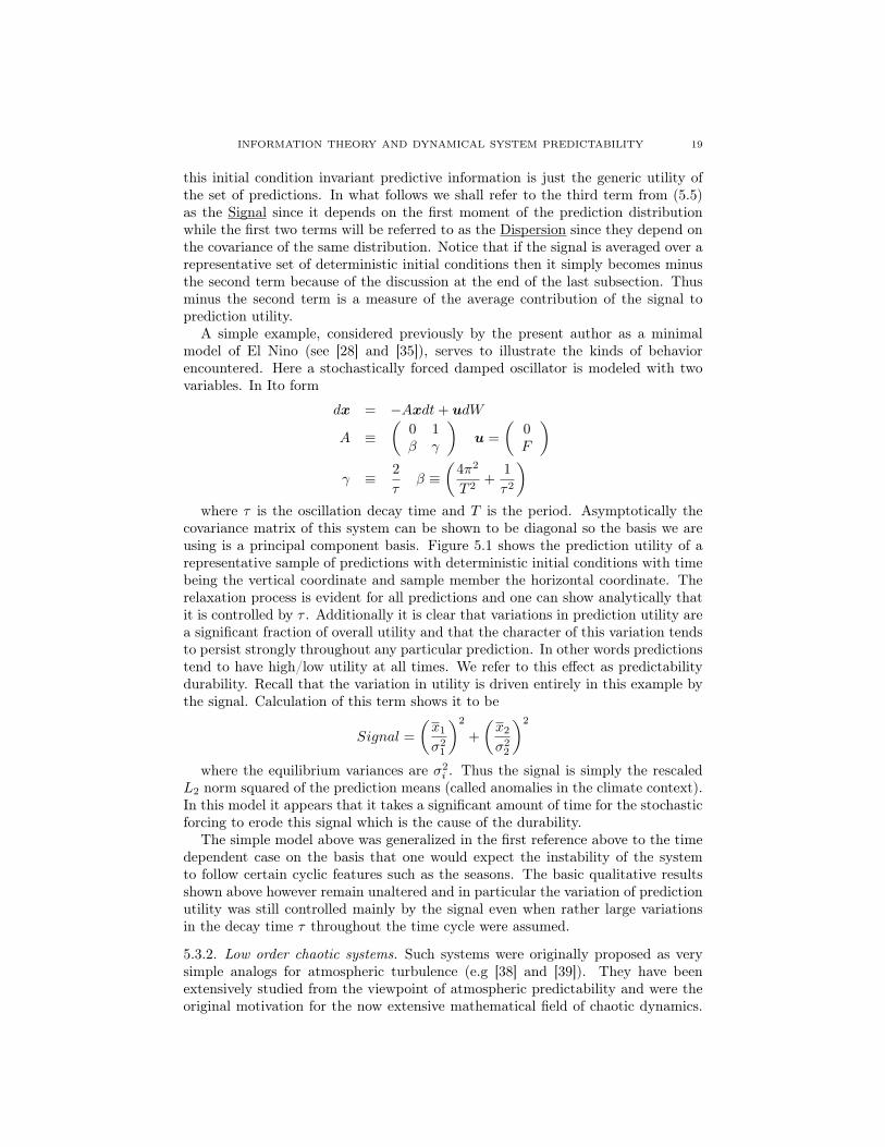
A simple example, considered previously by the present author as a minimalmodel of El Nino (see [28] and [35]), serves to illustrate the kinds of behaviorencountered. Here a stochastically forced damped oscillator is modeled with twovariables. In Ito form
dx = −Axdt+ udW
A ≡(
0 1β γ
)u =
(0F
)γ ≡ 2
τβ ≡
(4π2
T 2+
1
τ2
)where τ is the oscillation decay time and T is the period. Asymptotically the
covariance matrix of this system can be shown to be diagonal so the basis we areusing is a principal component basis. Figure 5.1 shows the prediction utility of arepresentative sample of predictions with deterministic initial conditions with timebeing the vertical coordinate and sample member the horizontal coordinate. Therelaxation process is evident for all predictions and one can show analytically thatit is controlled by τ . Additionally it is clear that variations in prediction utility area significant fraction of overall utility and that the character of this variation tendsto persist strongly throughout any particular prediction. In other words predictionstend to have high/low utility at all times. We refer to this effect as predictabilitydurability. Recall that the variation in utility is driven entirely in this example bythe signal. Calculation of this term shows it to be
Signal =
(x1
σ21
)2
+
(x2
σ22
)2
where the equilibrium variances are σ2i . Thus the signal is simply the rescaled
L2 norm squared of the prediction means (called anomalies in the climate context).In this model it appears that it takes a significant amount of time for the stochasticforcing to erode this signal which is the cause of the durability.
The simple model above was generalized in the first reference above to the timedependent case on the basis that one would expect the instability of the systemto follow certain cyclic features such as the seasons. The basic qualitative resultsshown above however remain unaltered and in particular the variation of predictionutility was still controlled mainly by the signal even when rather large variationsin the decay time τ throughout the time cycle were assumed.
5.3.2. Low order chaotic systems. Such systems were originally proposed as verysimple analogs for atmospheric turbulence (e.g [38] and [39]). They have beenextensively studied from the viewpoint of atmospheric predictability and were theoriginal motivation for the now extensive mathematical field of chaotic dynamics.

INFORMATION THEORY AND DYNAMICAL SYSTEM PREDICTABILITY 20
Figure 5.1. Prediction utility (relative entropy) for a series ofrepresentative initial conditions and at different prediction times.
Here, unlike the previous case, there is no great separation of timescales and thegrowth of small perturbations occurs through non-linear interaction of the degreesof freedom rather than from random forcing from fast neglected modes. Thesesystems are often characterized by an invariant measure that is fractal in character.This implies that the dimension of the space used to calculate probability densitiesis non-integral which means some care needs to be taken in defining appropriateentropic functionals. As noted earlier the non-linearity of the system but alsothe fractal equilibrium strange attractor mean that generally the best practicalapproach is Monte Carlo sampling with an appropriate coarse graining of statespace. One can for example define the entropy of the equilibrium strange attractoras
E = limM99K∞
limr99K0
E(M, r)
E(M, r) ≡ − 1
M
M∑i=1
ln
(Ni(r)
Mrd
)
= − 1
M
M∑i=1
ln
(Ni(r)
M
)+ d ln r ≡ S(M, r) + d ln r(5.6)
where Ni(r) is the number of attractor sample members within a radius r ofthe i’th sample member; d is the so-called fractional information dimension of theattractor andM is the number of sample points. Careful comparison with (2.1) and(2.2) shows this agrees with the usual definition up to a constant which multiplies
INFORMATION THEORY AND DYNAMICAL SYSTEM PREDICTABILITY 21
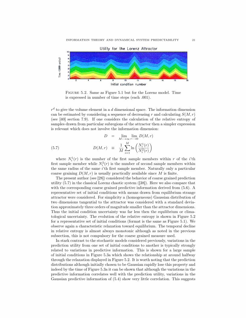
Figure 5.2. Same as Figure 5.1 but for the Lorenz model. Timeis expressed in number of time steps (each .001).
rd to give the volume element in a d dimensional space. The information dimensioncan be estimated by considering a sequence of decreasing r and calculating S(M, r)(see [40] section 7.9). If one considers the calculation of the relative entropy ofsamples drawn from particular subregions of the attractor then a simpler expressionis relevant which does not involve the information dimension:
D = limM99K∞
limr99K0
D(M, r)
D(M, r) ≡ 1
M
M∑i=1
ln
(N1
i (r)
N2i (r)
)(5.7)
where N1i (r) is the number of the first sample members within r of the i’th
first sample member while N2i (r) is the number of second sample members within
the same radius of the same i’th first sample member. Naturally only a particularcoarse graining D(M, r) is usually practically available since M is finite.
The present author (see [28]) considered the behavior of coarse grained predictionutility (5.7) in the classical Lorenz chaotic system ([38]). Here we also compare thatwith the corresponding coarse grained predictive information derived from (5.6). Arepresentative set of initial conditions with means drawn from equilibrium strangeattractor were considered. For simplicity a (homogeneous) Gaussian distribution oftwo dimensions tangential to the attractor was considered with a standard devia-tion approximately three orders of magnitude smaller than the attractor dimensions.Thus the initial condition uncertainty was far less then the equilibrium or clima-tological uncertainty. The evolution of the relative entropy is shown in Figure 5.2for a representative set of initial conditions (format is the same as Figure 5.1). Weobserve again a characteristic relaxation toward equilibrium. The temporal declinein relative entropy is almost always monotonic although as noted in the previoussubsection, this is not compulsory for the coarse grained measure used.
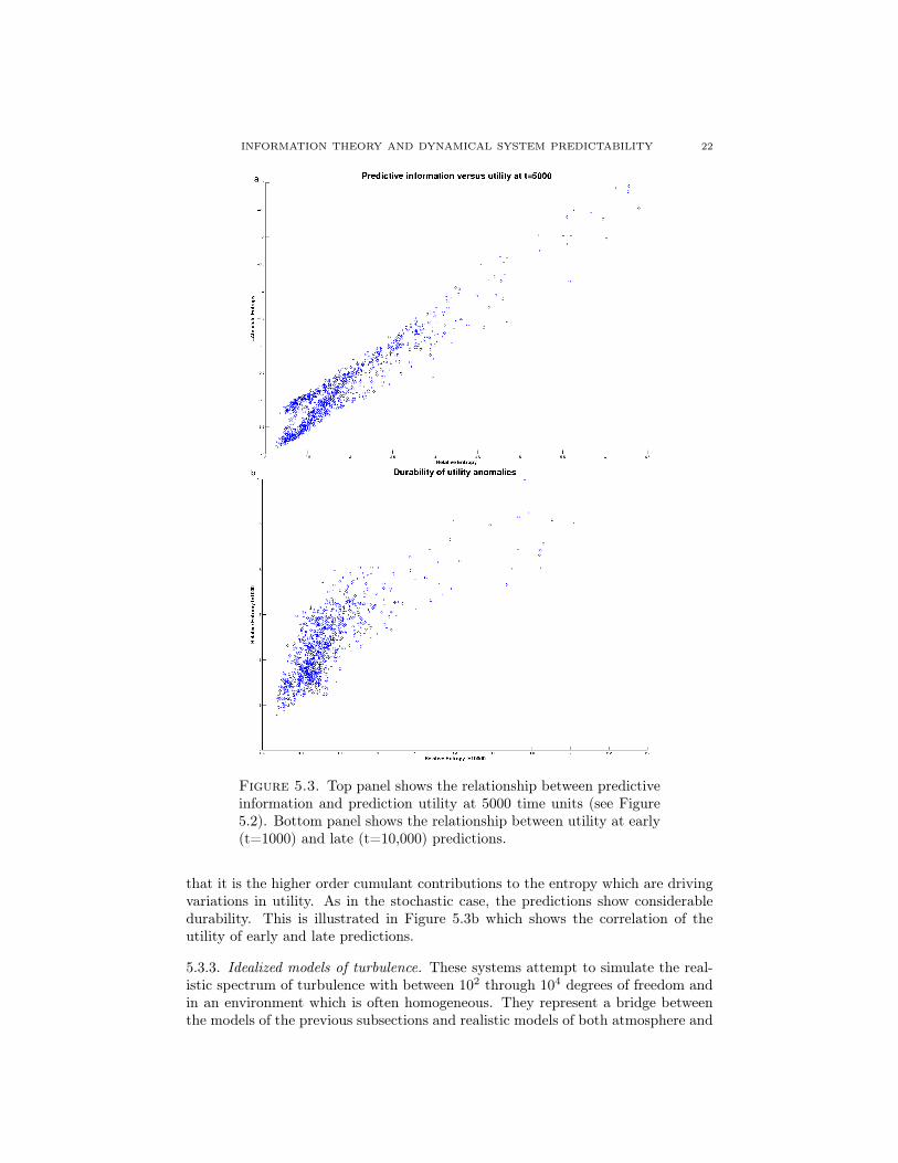
In stark contrast to the stochastic models considered previously, variations in theprediction utility from one set of initial conditions to another is typically stronglyrelated to variations in predictive information. This is shown for a large sampleof initial conditions in Figure 5.3a which shows the relationship at around halfwaythrough the relaxation displayed in Figure 5.2. It is worth noting that the predictiondistributions although initially chosen to be Gaussian rapidly lose this property andindeed by the time of Figure 5.3a it can be shown that although the variations in thepredictive information correlates well with the prediction utility, variations in theGaussian predictive information of (5.4) show very little correlation. This suggests
INFORMATION THEORY AND DYNAMICAL SYSTEM PREDICTABILITY 22
Figure 5.3. Top panel shows the relationship between predictiveinformation and prediction utility at 5000 time units (see Figure5.2). Bottom panel shows the relationship between utility at early(t=1000) and late (t=10,000) predictions.
that it is the higher order cumulant contributions to the entropy which are drivingvariations in utility. As in the stochastic case, the predictions show considerabledurability. This is illustrated in Figure 5.3b which shows the correlation of theutility of early and late predictions.
5.3.3. Idealized models of turbulence. These systems attempt to simulate the real-istic spectrum of turbulence with between 102 through 104 degrees of freedom andin an environment which is often homogeneous. They represent a bridge betweenthe models of the previous subsections and realistic models of both atmosphere and
INFORMATION THEORY AND DYNAMICAL SYSTEM PREDICTABILITY 23
ocean. The nature of the turbulence exhibited means that there is a large range oftimescales present and there are large non-linear transfers of energy between modesoften in the form of a scale cascade. Thus both the effects of the previous two typesof models are typically present.
Calculation of information theoretic functionals for models of this dimension in-volves essential difficulties. As we saw in the simple chaotic model above, the moststraightforward method involves a Monte Carlo method known as a prediction en-semble and some choice of coarse graining to estimate probability densities via apartitioning of state space. When we confront models with significantly higher di-mensions however this problem becomes very acute since the required number ofpartitions increases with the power of the dimension. In order to obtain a statis-tically reliable estimate of density for each partition we require that the ensemblesize be at least the same order as the number of partitions chosen. It is fairly clearthat only approximations to the functionals will be possible in such a situation.
Two approaches have been taken to this approximation problem. The first as-sumes that the ensemble is sufficiently large so that low order statistical momentscan be reliably calculated and then implicitly discards sample information regard-ing higher order moments as not known. One then uses the moment informationas a hard constraint on the hypothetical distribution and derives that distributionusing a maximum entropy hypothesis by deciding that no knowledge is availableregarding the higher order moments. In the case that only second order or lessmoments are available this implies, of course, that the hypothetical distributionis Gaussian. Typically however some higher order moments can also be reliablyestimated from prediction ensembles so a more general methodology is desirable.Under the appropriate circumstances, it is possible to solve for more general dis-tributions using a convex optimization methodology. This was originally suggestedby [41] and was developed extensively with the present application in mind by [42],[43], [44], [45] and [46].
In the latter references moments up to order four were typically retained and sogeneralized skewness and kurtosis statistics were assumed to be reliably estimatedfrom prediction ensembles. An interesting feature of these maximum entropy meth-ods is that as more moments are retained the relative entropy increases. Thus theGaussian relative entropy is bounded above by that derived from the more generaldistributions exhibiting kurtosis and skewness effects. This is analogous with thecoarse to fine graining hierarchy effect noted in the final paragraph of section 2.One feature of many models of turbulence makes this moment maximum entropyapproximation approach attractive: It is frequently observed that the low ordermarginal distributions are quasi Gaussian and so can usually be very well approxi-mated by retaining only the first four moments. Such a situation contrasts stronglywith that noted above in simple chaotic systems where highly non-Gaussian behav-ior is usual.
Another approach to the approximation issue (developed by the present authorin [47]) is to accept that only marginal distributions up to a certain low order aredefinable from a prediction ensemble. One then calculates the average relative en-tropy with respect to all possible marginal distributions and calls the result themarginal relative entropy. As in the maximum entropy case, the marginal rela-tive entropy of a certain order defined in this way strictly bounds from above themarginal relative entropies of lower order. This again is consistent with greater
INFORMATION THEORY AND DYNAMICAL SYSTEM PREDICTABILITY 24
retention of information as higher order marginal distributions are used to discrim-inate between distributions. Note also that at the top of this chain sits the fullrelative entropy.
An interesting aspect of these approximations is the role of the prediction ensem-ble in defining either the moment constraints or the marginal distributions. Somereflection on the matter shows that in fact these objects are subject to sample er-ror and this becomes larger as higher order approximations are considered. Thissuggests that in the first case the constraints assumed in deriving maximum en-tropy distributions should not be imposed as hard constraints but instead be weakconstraints as they should reflect the presence of the sample error. This rathersubtle issue has received little attention to date in the literature in the context ofmaximum entropy (see however [44]). See [47] for an information theoretic analysisfor the simpler marginal distribution estimation case.
Four different turbulence models of varying physical complexity and dimensionhave been analyzed in detail using the above approximation methods:
(1) A truncated version of Burgers equation detailed in [48]. This system is aone dimensional inviscid turbulence model with a set of conserved variableswhich enable a conventional Gibbs Gaussian equilibrium distribution. Pre-dictability issues relevant to the present discussion can be found in [49] and[43].
(2) The one dimensional Lorenz 1996 model of mid-latitude atmospheric turbu-lence detailed in [50]. This model exhibits a variety of different behaviorsdepending on the parameters chosen. For some settings strongly regularwave-like behavior is observed while for others a more irregular patternoccurs with some resemblance to atmospheric turbulence. The most un-stable linear modes of the system tend to have most weight at a particularwavenumber which is consistent with the observed atmosphere. Predictabil-ity issues from the present perspective can be found in [43].
(3) Two dimensional barotropic quasi-geostrophic turbulence detailed in, forexample, [51]. Barotropic models refer to systems with no vertical degreesof freedom. Quasi-geostrophic models are rotating fluids which filter outfast waves (both gravity and sound) in order to focus on low frequencyvariability. The barotropic versions aim at simulating very low frequencyvariability and exclude by design variability associated with mid-latitudestorms/eddies which have a typically shorter timescale. Predictability is-sues are discussed in [45] in the context of a global model with an inhomo-geneous background state.
(4) Baroclinic quasi-geostrophic turbulence as discussed in, for example, [52].This system is similar to the last except simple vertical structure is in-corporated which allows the fluid to draw energy from a vertical meanshear (baroclinic instability). These systems have therefore a representa-tion of higher frequency mid-latitude storms/eddies. This latter variabilityis sometimes considered to be approximately a stochastic forcing of thelow frequency barotropic variability although undoubtedly the turbulencespectrum is more complicated. Predictability issues from the present per-spective were discussed in [53] for a model with an homogeneous back-ground shear. They are discussed from a more conventional predictabilityviewpoint in [54].
INFORMATION THEORY AND DYNAMICAL SYSTEM PREDICTABILITY 25
Generally speaking for all systems the predictability time scale (as measured bythe prediction utility) is related to the equilibration time scale of the turbulencebeing considered. Variations in prediction utility with initial conditions are typi-cally similar to those seen in stochastic or simple chaotic systems. The origin ofthese variations is a rather complex subject and the answers obtained also varysignificantly according to the system examined. In the first subsection above weconsidered the case where both the prediction and equilibrium distributions wereGaussian. This meant that an analytical formula involving the lowest two momentswas possible and we found it convenient conceptually to separate terms into thosedependant on the first and second moments of prediction distribution which wereferred to as the signal and dispersion. It is important to emphasize however thatthis separation does not reflect a decomposition of the utility into the predictiveinformation (the uncertainty reduction of the prediction) and a remainder term.Indeed as we saw above, the second term of equation (5.5) which is included in thedispersion, is not at all related to uncertainty reduction but reflects differences inthe two distributions unrelated to entropy/uncertainty or their means.
When we move to the maximum entropy approximation for prediction utilityand consider moments of higher order it is possible to generalize this separation ofprediction moment contributions to the relative entropy into those dependent onthe prediction mean and those dependent on higher moments9. A comprehensiveand rigorous description of this generalized signal/dispersion decomposition is to befound in [43]. The contribution of these two terms was examined in this referencefor the first two turbulence systems listed above. The dominant contributor tooverall utility variations was found to depend on the parameters chosen for themodel as well as the prediction time chosen. There is also within this referencea discussion of when moments beyond the first two are important to a maximumentropy approximation retaining the first four moments.
When the higher order geostrophic turbulence models are considered (models 3and 4 in the list above), it is usual that a considerable fraction of the equilibriumvariability occurs due only to a relatively small number of modes. Predictabilitystudies have usually focused on the equilibration behavior of such modes.
In the study of a barotropic turbulence model [45] the focus was on the firstfour principal components of the equilibrium distribution. The maximum entropyframework retaining four moments was used and the variability of prediction utilityin terms of the generalized signal and dispersion examined with the conclusion thatdispersion was overwhelmingly responsible for variations.
A baroclinic turbulence model was studied in [53]. The equilibrium turbulencespectrum in such models is well known to be dominated energetically by the largescale vertically uniform (barotropic) modes (see [55]). The predictability studytherefore restricted attention to barotropic modes and the gravest four horizontalFourier modes. The marginal distributions for both prediction and equilibriumdistributions were observed to be quite close to Gaussian so only the first two mo-ments were retained for calculation of entropic functionals by the maximum entropymethod. In addition the marginal distributions with respect to these four dimen-sions was also calculated directly by a rather coarse partitioning. In contrast to
9Strictly speaking there are three contributions. One involves the prediction means; anotherthe higher order prediction moments alone and thirdly a cross term involving both. The authorscited in the text group this latter term with the first and call it the generalized signal.
INFORMATION THEORY AND DYNAMICAL SYSTEM PREDICTABILITY 26
the barotropic model above, variations in prediction utility were overwhelminglyrelated to variations in the (Gaussian) signal. This strong difference in predictabil-ity behavior has yet to be explained. It may be due to the importance in the lattercase of the stochastic like forcing of the low frequency barotropic modes by thehigher frequency baroclinic modes. These are of course absent in the barotropicturbulence case. Thus it may be that barotropic model is more like the low orderchaos case while the baroclinic model is more like the simple stochastic case. Thisis speculation however and deeper investigation is required.
5.3.4. Realistic global primitive equation models. Such models are simplified ver-sions of models used in real time to predict the daily weather. In contrast to mostmodels of the previous subsection, the background for the turbulence is very inho-mogeneous as it depends on geographical features such as topography and the jetstream. The latter is driven by the temperature gradient between the equator andpole and so peaks strongly in mid-latitudes. Compared with the quasi-geostrophicturbulence systems, more modes are generally required to explain the equilibriumvariance: Of order around 100 compared with less than 10 for the homogeneousbaroclinic quasi-geostrophic case. This dynamical situation has tended to limitthe application of the approximation approaches discussed earlier. The only studyconducted to date with such models from an information theoretic perspective wasby the present author in [56]. This used marginal relative entropies on the domi-nant 100 equilibrium modes10 as well as the Gaussian maximum entropy approachdiscussed above. Generally speaking, marginal distributions of dynamical variablestend to be close to Gaussian however this issue remains to be systematically inves-tigated. In the present context it was found that as initial conditions were varied,there was a correlation of order 0.8 between Gaussian estimates of relative entropyand those derived from marginal relative entropies. The latter tended to have ahigher correlation among themselves.
In this system, the equilibration time scale implied by the above estimates ofprediction utility is a strong inverse function of the amount of mean vertical shearpresent in the atmosphere. When this shear is strong as it is during winter itis between 1 and 2 months while for the summer weak shear case it is around 3months. These estimates of predictability are significantly longer than those derivedfrom practical weather prediction where two weeks is generally accepted to be thecurrent predictability limit. This difference may be due to model error of practicalpredictions and/or due to simplifications present in the model studied in [56] whichexcludes important random processes such as moist convection which can providea significant mechanism to reduce predictability.
The variation in prediction utility with respect to a representative set of initialconditions was also studied and the results found were somewhat similar to thosenoted in the baroclinic turbulence model discussed earlier. Overall relative entropyfluctuations (either Gaussian or marginal) were most strongly related to signalrather than dispersion variations. This effect was more pronounced for short rangerather than long range predictions. The dispersion was however also related toutility but at a lower level than signal. Like both the stochastic and simple chaoticmodels discussed earlier, prediction utility variations tended to show durability i.e.
10Practical prediction ensemble sizes restrict marginal relative entropies to order four or less.
INFORMATION THEORY AND DYNAMICAL SYSTEM PREDICTABILITY 27
high utility predictions tended to remain high throughout a prediction and viceversa.
5.3.5. Other recent applications. There have been interesting applications of thefunctionals discussed here to various climate prediction problems. This has beenaided by the fact that to an even greater extent than the turbulence models dis-cussed above, the marginal distributions observed tend to be very close to Gaussian.Indeed it is almost as if a central limit theorem operates in many complex geophys-ical models in such a way that many distributions of dynamical variables of interesttend to be approximately normal.
The El Nino coupled ocean/atmosphere system was considered in depth withrealistic models in [57] and conclusions were broadly in line with the simple sto-chastic models considered earlier. In general the signal rather than dispersion playeda larger role in explaining predictability variation.
The problem of global warming projection was considered from the current per-spective by [58]. They used the relative entropy between the equilibrium distribu-tion of various models and the present observed climate/equilibrium distributionas a measure of the veracity of a particular model. They then found a relationshipbetween this veracity and the amplitude of projected global average warming overthe next century. Models with higher veracity tended to project greater warm-ing. In related work, global warming model errors were analyzed using an array ofempirical information theoretic tools in [59]. This allowed the authors to identifyglobal warming patterns of highest sensitivity.
Part of the issue of long term climate projection concerns its separation into thatdue to ocean initial conditions (natural decadal variability) and that due to changesin forcing due to the radiative effects of greenhouse gases. This issue was addressedusing relative entropy measures of predictability in [60] where it was found that thepredictability switches from the first kind to the second kind at leads of roughly5-10 years.
The predictability of the natural decadal predictability mentioned above wasanalyzed in detail using relative entropy measures in [61]. A focus was on thebehavior of the first few principal components and the authors used the Gaussiansignal/dispersion decomposition to carefully analyze the nature of this predictabilityand the way it transfers between principal components as predictions evolve.
Finally the Gaussian signal/dispersion decomposition of relative entropy hasbeen used to study the nature of the predictability of polar sea ice in a very recentstudy by C. Bitz and coworkers at the University of Washington (private commu-nication to the author).
6. Conclusions and Outlook
Predictability issues in dynamical models are studied very naturally using in-formation theoretic functionals. This follows because such variables are best con-sidered to be random variables and entropic functionals have a very intuitive in-terpretation in terms of uncertainty and as measures of the differences betweendistributions. Adding to this attraction is the fact that these functionals exhibitinvariance under general transformations of the variables describing the dynamicalsystem and that they have deep connections with concepts from statistical physics.Indeed it is argued in this review that the utility of a prediction can be measuredby the degree of statistical disequilibrium within the system. Thus the study of the

INFORMATION THEORY AND DYNAMICAL SYSTEM PREDICTABILITY 28
predictability of a system is equivalent to the study of the nature of its statisticalequilibration.
Application of the concepts considered here has often relied on the fact that therandom variables under study are quasi-Gaussian since this allows application ofanalytical expressions. It should be emphasized however (and we saw this in Section4) that a major attraction of information theory is the ability to go beyond thissituation and consider highly non-linear and non-Gaussian distributions. As we sawin detail in section 5 considerable progress has been made using maximum entropymethods to improve approximate calculation of functionals in high dimensionalsystem. No doubt however more work remains in this challenging area where thecurse of dimensionality always lurks.
The fundamental mechanism that drives equilibration and hence loss of pre-dictability is the dynamical process which leads to statistical irreversibility. This,as we saw in Section 3, is intimately related to the manner in which a systemis coarse grained and fundamental progress in that area will drive a deeper un-derstanding of system predictability. Thus the expectation of the author is thatfurther progress in the area of non-equilibrium statistical mechanics will be of greatbenefit to the study of the basic nature of prediction.
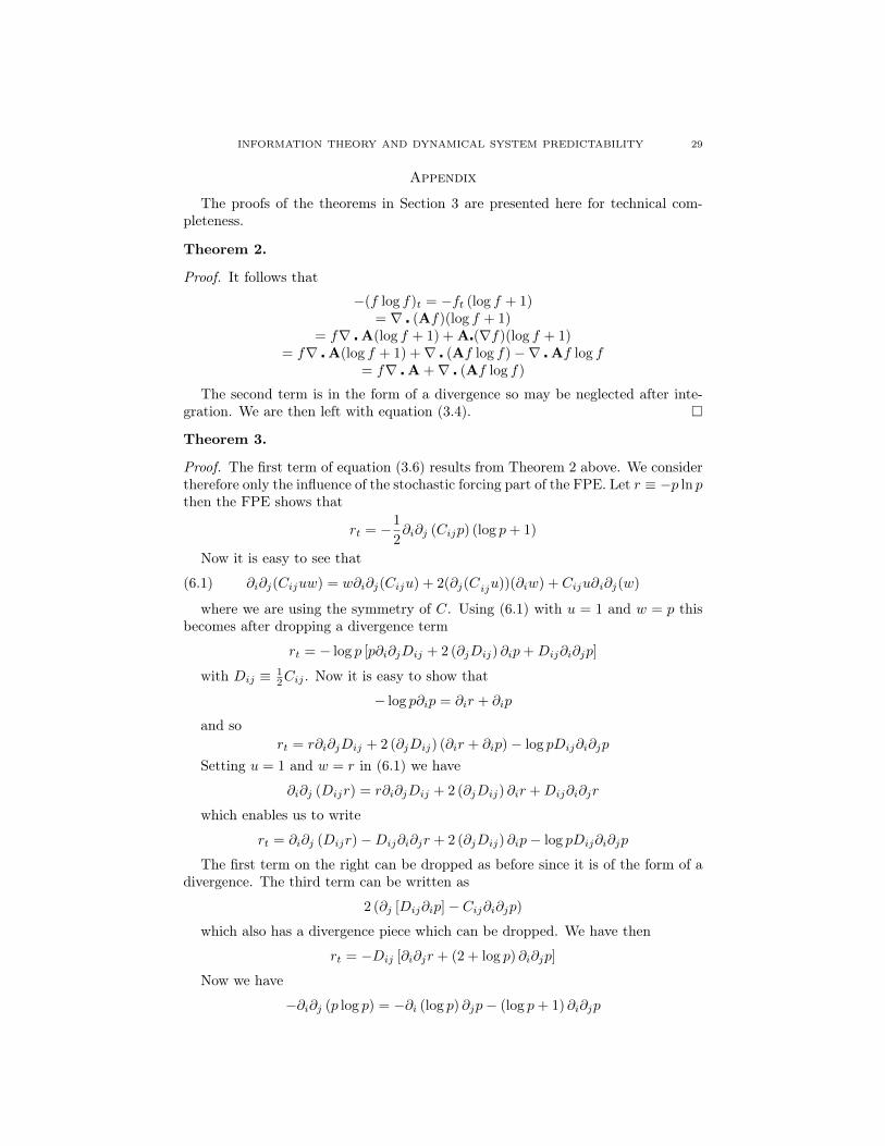
INFORMATION THEORY AND DYNAMICAL SYSTEM PREDICTABILITY 29
Appendix
The proofs of the theorems in Section 3 are presented here for technical com-pleteness.
Theorem 2.
Proof. It follows that
−(f log f)t = −ft (log f + 1)= ∇ � (Af)(log f + 1)
= f∇ �A(log f + 1) + A�(∇f)(log f + 1)= f∇ �A(log f + 1) +∇ � (Af log f)−∇ �Af log f
= f∇ �A +∇ � (Af log f)
The second term is in the form of a divergence so may be neglected after inte-gration. We are then left with equation (3.4). �
Theorem 3.
Proof. The first term of equation (3.6) results from Theorem 2 above. We considertherefore only the influence of the stochastic forcing part of the FPE. Let r ≡ −p ln pthen the FPE shows that
rt = −1
2∂i∂j (Cijp) (log p+ 1)
Now it is easy to see that
(6.1) ∂i∂j(Cijuw) = w∂i∂j(Ciju) + 2(∂j(Ciju))(∂iw) + Ciju∂i∂j(w)
where we are using the symmetry of C. Using (6.1) with u = 1 and w = p thisbecomes after dropping a divergence term
rt = − log p [p∂i∂jDij + 2 (∂jDij) ∂ip+Dij∂i∂jp]
with Dij ≡ 12Cij . Now it is easy to show that
− log p∂ip = ∂ir + ∂ip
and sort = r∂i∂jDij + 2 (∂jDij) (∂ir + ∂ip)− log pDij∂i∂jp
Setting u = 1 and w = r in (6.1) we have
∂i∂j (Dijr) = r∂i∂jDij + 2 (∂jDij) ∂ir +Dij∂i∂jr
which enables us to write
rt = ∂i∂j (Dijr)−Dij∂i∂jr + 2 (∂jDij) ∂ip− log pDij∂i∂jp
The first term on the right can be dropped as before since it is of the form of adivergence. The third term can be written as
2 (∂j [Dij∂ip]− Cij∂i∂jp)
which also has a divergence piece which can be dropped. We have then
rt = −Dij [∂i∂jr + (2 + log p) ∂i∂jp]
Now we have
−∂i∂j (p log p) = −∂i (log p) ∂jp− (log p+ 1) ∂i∂jp
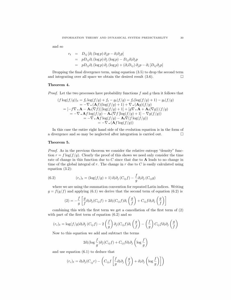
INFORMATION THEORY AND DYNAMICAL SYSTEM PREDICTABILITY 30
and so
rt = Dij [∂i (log p) ∂jp− ∂i∂jp]= pDij∂i (log p) ∂j (log p)−Dij∂i∂jp
= pDij∂i (log p) ∂j (log p) + (∂iDij) ∂jp− ∂i [Dij∂jp]
Dropping the final divergence term, using equation (3.5) to drop the second termand integrating over all space we obtain the desired result (3.6). �
Theorem 4.
Proof. Let the two processes have probability functions f and g then it follows that
(f log(f/g))t = ft log(f/g) + ft − gt(f/g) = ft(log(f/g) + 1)− gt(f/g)= −∇ � (Af)(log(f/g) + 1) +∇ � (Ag)(f/g)
= [−f∇ �A−A�(∇f)] [log(f/g) + 1] + [g∇ �A + A�(∇g)] (f/g)= −∇ �Af log(f/g)−A�(∇f [log(f/g) + 1]−∇g(f/g))
= −∇ �Af log(f/g)−A�∇(f log(f/g))= −∇ � (Af log(f/g))
In this case the entire right hand side of the evolution equation is in the form ofa divergence and so may be neglected after integration is carried out. �
Theorem 5.
Proof. As in the previous theorem we consider the relative entropy “density” func-tion r = f log(f/g). Clearly the proof of this shows we need only consider the timerate of change in this function due to C since that due to A leads to no change intime of the global integral of r. The change in r due to C is easily calculated usingequation (3.2):
(6.2) (rc)t = (log(f/g) + 1) ∂i∂j (Cijf)− f
g∂i∂j (Cijg)
where we are using the summation convention for repeated Latin indices. Writingg = f(g/f) and applying (6.1) we derive that the second term of equation (6.2) is
(2) = −fg
[g
f∂i∂j(Cijf) + 2∂i(Cijf)∂i
(g
f
)+ Cijf∂i∂j
(g
f
)]combining this with the first term we get a cancellation of the first term of (2)
with part of the first term of equation (6.2) and so
(rc)t = log(f/g)∂i∂j (Cijf)− 2
(f
g
)∂j(Cijf)∂i
(g
f
)−(f
g
)Cijf∂i∂j
(g
f
)Now to this equation we add and subtract the terms
2∂i(logf
g)∂j(Cijf) + Cijf∂i∂j
(log
f
g
)and use equation (6.1) to deduce that
(rc)t = ∂i∂j(Cijr)−(Cijf
[f
g∂i∂j
(g
f
)+ ∂i∂j
(log
f
g
)])
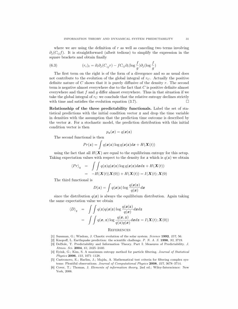
INFORMATION THEORY AND DYNAMICAL SYSTEM PREDICTABILITY 31
where we are using the definition of r as well as canceling two terms involving∂j(Cijf). It is straightforward (albeit tedious) to simplify the expression in thesquare brackets and obtain finally
(6.3) (rc)t = ∂i∂j(Cijr)− fCij∂i(logf
g)∂j(log
f
g)
The first term on the right is of the form of a divergence and so as usual doesnot contribute to the evolution of the global integral of rC . Actually the positivedefinite nature of C shows that it is purely diffusive of the density r. The secondterm is negative almost everywhere due to the fact that C is positive definite almosteverywhere and that f and g differ almost everywhere. Thus in that situation if wetake the global integral of rC we conclude that the relative entropy declines strictlywith time and satisfies the evolution equation (3.7). �
Relationship of the three predictability functionals. Label the set of sta-tistical predictions with the initial condition vector z and drop the time variablein densities with the assumption that the prediction time outcome is described bythe vector x. For a stochastic model, the prediction distribution with this initialcondition vector is then
pz(x) = q(x|z)
The second functional is then
Pr(z) =
ˆq(x|z) log q(x|z)dx +H(X(t))
using the fact that all H(X) are equal to the equilibrium entropy for this setup.Taking expectation values with respect to the density for z which is q(z) we obtain
〈Pr〉q =
ˆ ˆq(z)q(x|z) log q(x|z)dxdz +H(X(t))
= −H(X(t)|X(0)) +H(X(t)) = I(X(t);X(0)
The third functional is
D(z) =
ˆq(x|z) log
q(x|z)
q(x)dx
since the distribution q(x) is always the equilibrium distribution. Again takingthe same expectation value we obtain
〈D〉q =
ˆ ˆq(z)q(x|z) log
q(x|z)
q(x)dxdz
=
ˆ ˆq(x, z) log
q(x, z)
q(z)q(x)dxdz = I(X(t);X(0))
References
[1] Sussman, G.; Wisdom, J. Chaotic evolution of the solar system. Science 1992, 257, 56.[2] Knopoff, L. Earthquake prediction: the scientific challenge. P. N. A. S. 1996, 93, 3719.[3] DelSole, T. Predictability and Information Theory. Part I: Measures of Predictability. J.
Atmos. Sci. 2004, 61, 2425–2440.[4] Eyink, G.; Kim, S. A maximum entropy method for particle filtering. Journal of Statistical
Physics 2006, 123, 1071–1128.[5] Castronovo, E.; Harlim, J.; Majda, A. Mathematical test criteria for filtering complex sys-
tems: Plentiful observations. Journal of Computational Physics 2008, 227, 3678–3714.[6] Cover, T.; Thomas, J. Elements of information theory, 2nd ed.; Wiley-Interscience: New
York, 2006.

INFORMATION THEORY AND DYNAMICAL SYSTEM PREDICTABILITY 32
[7] Amari, S.; Nagaoka, H. Methods of Information Geometry; Translations of MathematicalMonographs, AMS, Oxford University Press, 2000.
[8] Daems, D.; Nicolis, G. Entropy production and phase space volume contraction. Phys. Rev.E 1999, 59, 4000–4006.
[9] Garbaczewski, P. Differential entropy and dynamics of uncertainty. J. Stat. Phys. 2006,123, 315–355.
[10] Ruelle, D. Positivity of entropy production in nonequilibrium statistical mechanics. Journalof Statistical Physics 1996, 85, 1–23.
[11] Lebowitz, J.; Bergmann, P. Irreversible gibbsian ensembles. Annals of Physics 1957, 1, 1–23.[12] Gardiner, C.W. Handbook of Stochastic Methods for Physics, Chemistry and the Natural
Sciences; Vol. 13, Springer Series in Synergetics, Springer, 2004.[13] Kaneko, K. Lyapunov analysis and information flow in coupled map lattices. Physica D 1986,
23, 436.[14] Vastano, J.A.; Swinney, H.L. Information transport in spatiotemporal systems. Phys. Rev.
Lett. 1988, 60, 1773.[15] Schreiber, T. Spatiotemporal structure in coupled map lattices: Two point correlations versus
mutual information. J. Phys. 1990, A23, L393–L398.[16] Schreiber, T. Measuring Information Transfer. Phys. Rev. Lett. 2000, 85, 461–464.[17] Liang, X.S.; Kleeman, R. Information transfer between dynamical system components. Phys.
Rev. Lett. 2005, 95, 244101.[18] Liang, X.S.; Kleeman, R. A rigorous formalism of information transfer between dynamical
system components I. Discrete maps. Physica D. 2007, 231, 1–9.[19] Liang, X.S.; Kleeman, R. A rigorous formalism of information transfer between dynamical
system components II. Continuous flow. Physica D. 2007, 227, 173–182.[20] Majda, A.J.; Harlim, J. Information flow between subspaces of complex dynamical systems.
Proceedings National Academy of Science 2007, 104, 9558–9563.[21] Zubarev, D.; Morozov, V.; Ropke, G. Statistical mechanics of nonequilibrium processes. Vol.
1: Basic concepts, kinetic theory 1996.[22] Palmer, T.N.; Gelaro, R.; Barkmeijer, J.; Buizza, R. Singular vectors, metrics, and adaptive
observations. J. Atmos. Sci. 1998, 55, 633–653.[23] Bishop, C.; Etherton, B.; Majumdar, S. Adaptive sampling with the ensemble transform
Kalman filter. Part I: Theoretical aspects. Mon. Weath. Rev. 2001, 129, 420–436.[24] Kleeman, R. Information flow in ensemble weather predictions. J. Atmos Sci. 2007, 64, 1005–
1016.[25] Jolliffe, I.; Stephenson, D. Forecast verification: a practitioner’s guide in atmospheric science;
Wiley, 2003.[26] Leung, L.Y.; North, G.R. Information Theory and Climate Prediction. J. Clim. 1990, 3, 5–
14.[27] Schneider, T.; Griffies, S. A conceptual framework for predictability studies. J. Clim. 1999,
12, 3133–3155.[28] Kleeman, R. Measuring dynamical prediction utility using relative entropy. J. Atmos. Sci.
2002, 59, 2057–2072.[29] Roulston, M.S.; Smith, L.A. Evaluating Probabilistic Forecasts Using Information Theory.
Mon. Weath. Rev. 2002, 130, 1653–1660.[30] Bernardo, J.; Smith, A. Bayesian Theory; John Wiley and Sons, 1994.[31] Kleeman, R.; Moore, A.M. A new method for determining the reliability of dynamical ENSO
predictions. Mon. Weath. Rev. 1999, 127, 694–705.[32] Hasselmann, K. Stochastic climate models. Part I. Theory. Tellus 1976, 28, 473–485.[33] Kleeman, R.; Power, S. Limits to predictability in a coupled ocean-atmosphere model due to
atmospheric noise. Tellus A 1994, 46, 529–540.[34] Penland, C.; Sardeshmukh, P. The optimal growth of tropical sea surface temperature anom-
alies. J. Clim. 1995, 8, 1999–2024.[35] Kleeman, R. Spectral analysis of multi-dimensional stochastic geophysical models with an
application to decadal ENSO variability. J. Atmos. Sci. 2010. To appear.[36] Saravanan, R.; McWilliams, J. Advective ocean–atmosphere interaction: An analytical sto-
chastic model with implications for decadal variability. Journal of Climate 1998, 11, 165–188.[37] DelSole, T.; Farrel, B.F. A stochastically excited linear system as a model for quasigeostrophic
turbulence: analytic results for one- and two-layer fluids. J. Atmos. Sci. 1995, 52, 2531–2547.

INFORMATION THEORY AND DYNAMICAL SYSTEM PREDICTABILITY 33
[38] Lorenz, E.N. Deterministic non-periodic flows. J. Atmos. Sci. 1963, 20, 130–141.[39] Lorenz, E.N. Irregularity: a fundamental property of the atmosphere. Tellus 1984, 36A, 98–
110.[40] Nayfeh, A.; Balachandran, B. Applied nonlinear dynamics; Vol. 2, Wiley Online Library,
1995. 685 pp.[41] Mead, L.R.; Papanicolaou, N. Maximum entropy in the problem of moments. J. Math. Phys.
1984, 25, 2404–2417.[42] Majda, A.J.; Kleeman, R.; Cai, D. A framework of predictability through relative entropy.
Meth. Appl. Anal. 2002, 9, 425–444.[43] Abramov, R.; Majda, A. Quantifying uncertainty for non-Gaussian ensembles in complex
systems. SIAM Journal on Scientific Computing 2005, 26, 411–447.[44] Haven, K.; Majda, A.; Abramov, R. Quantifying Predictability Through Information Theory:
Small Sample Estimation in a Non-Gaussian Framework. J. Comp. Physics 2004. Submitted.[45] Abramov, R.; Majda, A.; Kleeman, R. Information Theory and Predictability for Low Fre-
quency Variability. J. Atmos Sci 2005, 62, 65–87.[46] Abramov, R. A practical computational framework for the multidimensional moment-
constrained maximum entropy principle. Journal of Computational Physics 2006, 211, 198–209.
[47] Kleeman, R. Statistical predictability in the atmosphere and other dynamical systems. Phys-ica D 2007, 230, 65–71.
[48] Majda, A.J.; Timofeyev, I. Statistical mechanics for truncations of the Burgers-Hopf equation:a model for intrinsic stochastic behavior with scaling. Milan Journal of Mathematics 2002,70(1), 39–96.
[49] Kleeman, R.; Majda, A.J.; Timofeyev, I. Quantifying predictability in a model with statisticalfeatures of the atmosphere. Proc. Nat. Acad. Sci. USA 2002, 99, 15291–15296.
[50] Lorenz, E. Predictability: A problem partly solved. Proc. Seminar on Predictability, 1996,Vol. 1, pp. 1–18.
[51] Selten, F. An efficient description of the dynamics of barotropic flow. J. Atmos. Sci. 1995,52, 915–936.
[52] Salmon, R. Baroclinic instability and geostrophic turbulence. Geophys. Astrophys. Fluid Dyn.1980, 15, 167–211.
[53] Kleeman, R.; Majda, A.J. Predictability in a model of geostrophic turbulence. J. Atmos Sci2005, 62, 2864–2879.
[54] Vallis, G.K. On the predictability of Quasi-Geostrophic Flow: The Effects of Beta and Baro-clinicity. J. Atmos. Sci. 1983, 40, 10–27.
[55] Salmon, R. Lectures on Geophysical Fluid Dynamics; Oxford Univ. Press, New York, 1998.[56] Kleeman, R. Limits, variability and general behaviour of statistical predictability of the mid-
latitude atmosphere. J. Atmos Sci 2008, 65, 263–275.[57] Tang, Y.; Kleeman, R.; Moore, A. Comparison of Information-based Measures of Forecast
Uncertainty in Ensemble ENSO Prediction. J. Clim. 2008, 21, 230–247.[58] Shukla, J.; DelSole, T.; Fennessy, M.; Kinter, J.; Paolino, D. Climate model fidelity and
projections of climate change. Geophys. Res. Lett 2006, 33, L07702.[59] Majda, A.; Gershgorin, B. Quantifying uncertainty in climate change science through empir-
ical information theory. Proceedings of the National Academy of Sciences 2010, 107, 14958.[60] Branstator, G.; Teng, H. Two Limits of Initial-value Decadal Predictability in a CGCM.
Journal of Climate 2010.[61] Teng, H.; Branstator, G. Initial-value predictability of prominent modes of North Pacific
subsurface temperature in a CGCM. Climate Dynamics 2010, pp. 1–22.
Acknowledgements
The author wishes to thank the Isaac Newton Institute at Cambridge Universitywhere this review was written during a visit in August 2010. Stimulating discussionsover the past few years with Tim DelSole, Greg Eyink, Andy Majda, Ilya Timofeyevand Bruce Turkington are gratefully acknowledged. Support from the NationalScience foundation from a variety of grants is also gratefully acknowledged.
Courant Institute of Mathematical Sciences, New York University, New York