Market Competition and Price Discrimination the Case of Ketchup

8/13/2019 Market Competition and Price Discrimination the Case of Ketchup

http://slidepdf.com/reader/full/market-competition-and-price-discrimination-the-case-of-ketchup 1/31

Market Competition and Price Discrimination: The

Case of Ketchup

Congnan Zhany

November 2012

Abstract

In this paper, using a two-way …xed e¤ects approach, I examine the relationship

between market competition and second-degree price discrimination in the ketchup

market. Results show price discrimination increases as market competition intensi-

…es. The results are robust to di¤erent de…nitions of price discrimination and di¤erent

measures of market competition.

Keywords: Price Discrimination, Market Concentration, Ketchup

JEL Classi…cations: L11; L66

I thank Brian McManus, Wally Thurman, Tomislav Vukina and Xiaoyong Zheng for helpful comments

and suggestions. All remaining errors are my own.yDepartment of Economics, North Carolina State University, NCSU Campus Box 8110, Raleigh, NC

27695. Email: [email protected].



1 Introduction

Price discrimination is a practice …rms often use to extract consumer surplus from high-valuation customers. Though its e¤ect on total welfare can be either positive or negative,

it usually bene…ts the producers at the cost of the consumers. Economists have long been

interested in this phenomenon (e.g. chapter 3 of Tirole 1988, Stole 2007). One of the

main issues in this literature is the relationship between market structure and the ability or

the incentives of …rms to practice price discrimination. The conventional wisdom is that a

competitive …rm cannot price discriminate because it is a price taker and a …rm with market

power can price discriminate as long as it can segment consumers.However, both theoretical studies by Katz (1984), Borenstein (1985), Holmes (1989) and

Dana (1998) and empirical studies by Shepard (1991) and Graddy (1995) show that price

discrimination can exist in quite competitive markets. And more recently, Hernandez and

Wiggins (2008), Yang and Ye (2008) and Dai, Liu and Serfes (2010) study second-degree

price discrimination models where the relationship between market competition and price

discrimination is positive and nonlinear, respectively, instead of negative. Finally, McAfee,

Mialon and Mialon (2006) show that the same relationship can be either positive or negativeusing a third-degree price discrimination model. Hernandez (2011) explains the intuition for

why price discrimination may actually increase when …rms face more competition. In his

model, when competition intensi…es, the prices of both low- and high-quality products fall as

…rms have less market power, but the price of a low-quality product decreases proportionately

more than that of a high-quality product, that is, …rms compete more intensively for the low-

valuation customers. This is because in his model, …rms have to concede to high-valuation

consumers higher informational rents when they purchase the high-quality product than when

they purchase the low-quality product (so that they purchase the high-quality product). With

increased competition, …rms worry less about providing additional rents to high-valuation

consumers as the rents they enjoy increase with competition. As a result, they cut price less

for the high quality product.

Because theoretical studies do not produce a clear prediction, the relationship between

1



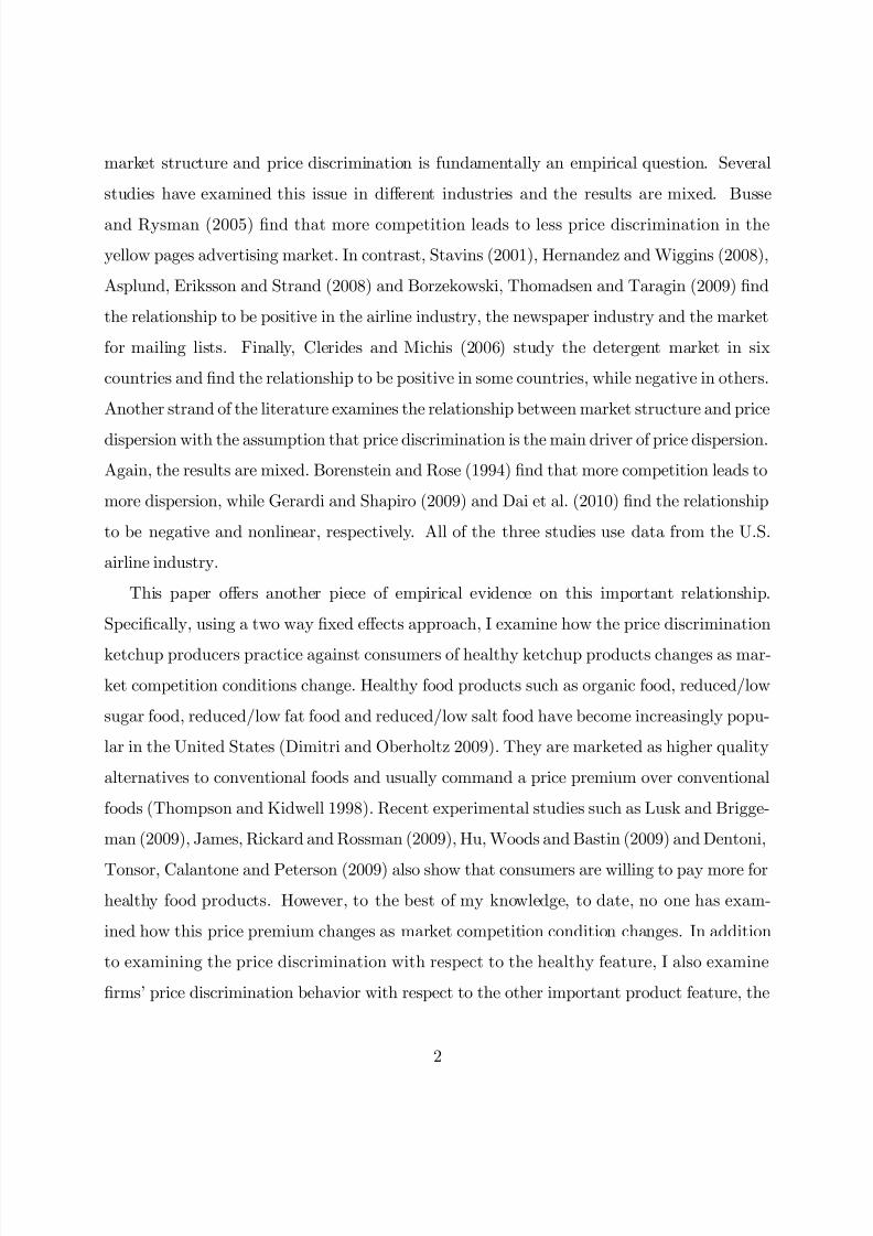
market structure and price discrimination is fundamentally an empirical question. Several

studies have examined this issue in di¤erent industries and the results are mixed. Busse

and Rysman (2005) …nd that more competition leads to less price discrimination in the

yellow pages advertising market. In contrast, Stavins (2001), Hernandez and Wiggins (2008),

Asplund, Eriksson and Strand (2008) and Borzekowski, Thomadsen and Taragin (2009) …nd

the relationship to be positive in the airline industry, the newspaper industry and the market

for mailing lists. Finally, Clerides and Michis (2006) study the detergent market in six

countries and …nd the relationship to be positive in some countries, while negative in others.

Another strand of the literature examines the relationship between market structure and price

dispersion with the assumption that price discrimination is the main driver of price dispersion.

Again, the results are mixed. Borenstein and Rose (1994) …nd that more competition leads to

more dispersion, while Gerardi and Shapiro (2009) and Dai et al. (2010) …nd the relationship

to be negative and nonlinear, respectively. All of the three studies use data from the U.S.

airline industry.

This paper o¤ers another piece of empirical evidence on this important relationship.

Speci…cally, using a two way …xed e¤ects approach, I examine how the price discrimination

ketchup producers practice against consumers of healthy ketchup products changes as mar-

ket competition conditions change. Healthy food products such as organic food, reduced/low

sugar food, reduced/low fat food and reduced/low salt food have become increasingly popu-

lar in the United States (Dimitri and Oberholtz 2009). They are marketed as higher quality

alternatives to conventional foods and usually command a price premium over conventional

foods (Thompson and Kidwell 1998). Recent experimental studies such as Lusk and Brigge-

man (2009), James, Rickard and Rossman (2009), Hu, Woods and Bastin (2009) and Dentoni,

Tonsor, Calantone and Peterson (2009) also show that consumers are willing to pay more for

healthy food products. However, to the best of my knowledge, to date, no one has exam-

ined how this price premium changes as market competition condition changes. In addition

to examining the price discrimination with respect to the healthy feature, I also examine

…rms’ price discrimination behavior with respect to the other important product feature, the

2



package size.

Another contribution of this study comes from the data and the econometric model used.

The dataset used is a panel dataset. This allows me to use a two-way …xed e¤ects approach,

which controls for both the product …xed e¤ects which are invariant across di¤erent markets,

as well as the …rm and market interaction …xed e¤ects, which are invariant across products by

the same …rm in the same market, in the regression analysis.1 Examining price discrimination

empirically has been a di¢cult task because price discrimination is de…ned as price-cost

margins or markups between di¤erent products, while usually only price data are observed.

Therefore, how credible the results of a study are depends on whether the researcher does a

good job of controlling for cost factors in the regression analysis. The two-way …xed e¤ects

approach I use control for unobserved product, …rm and market speci…c cost shifters, in

addition to controlling for the observed ones. Therefore, my study is less likely to su¤er from

the omitted variable bias problem. None of the empirical price discrimination studies cited

above employs such an approach.

The results indicate that price discrimination with respect to both the healthy feature

and package size increases when competition intensi…es in the ketchup market. The results

are robust to di¤erent de…nitions of price discrimination and di¤erent measures of market

competition. This implies that the change in market competition has e¤ects on both price

levels and the relative price structure of high- and low-quality ketchup products. These

results are consistent with the theoretical implications of the Hernandez (2011) model.

The rest of the paper is organized as follow. Section two describes the data, while Section

three details the empirical strategy. Results are presented and discussed in Section four and

the …nal Section concludes.

1 Note that the …rm and market interaction …xed e¤ects are more general than controlling for …rm and

market …xed e¤ects individually.

3



2 Industry and Data

The US ketchup market is selected for analysis because of data availability. Healthy ororganic fresh produce is the top selling category of healthy foods (Dimitri and Oberholtzer

2009). However, brand or …rm level price and sales data for such products are simply not

available. For the ketchup market, on the other hand, brand level price and sales scanner

data are collected by marketing companies and are available to researchers.

Ketchup is a widely used condiment in the US, found in 97% of all kitchens, a showing

matched only by salt, pepper, and sugar (Villas-Boas and Zhao 2005). It is mainly consumed

with hot dogs, French fries, hamburgers, pasta and serves as seasoning when making saucessuch as salsa and other food. Heinz is the leading …rm whose market share remains stable

around 60% in volume in recent years. Hunt’s, a ConAgra Foods brand, is the second largest,

accounting for about 16% of the market. The rest of the market is shared by Del Monte,

private label products, and other local brands.

The business section of the annual reports of Heinz and ConAgra Foods provide a glimpse

of the ketchup business ranging from procurement of inputs to retailing of outputs. Ketchup

recipes are developed in individual company’s research laboratories and experimental kitchens.Then, ingredients are procured, inspected and transported to factories. To hedge against the

spot market price volatility, major ketchup producers usually sign futures contracts with

farmers growing raw materials such as tomatoes, cucumbers and onions. Ingredients such as

sugar and sweeteners (high fructose corn syrup, a major sugar substitute in most of Heinz

and Hunt’s products) are purchased from approved suppliers. In the factory, raw materials

are manufactured into ketchup products using the following sequence of processes: steriliza-

tion, homogenization, chilling, freezing, pickling, drying, freeze drying, baking or extruding,

bottling and labeling. Products are sold through their own sales organizations and through

independent brokers, agents and distributors to chain, wholesale and other retailers. Wal-

Mart is the number one customer of Heinz and ConAgra Foods, representing approximately

11% and 18% of the …rms total sales in 2010.

4



2.1 Raw Data

The data set used in this paper is the Information Resources, Inc. (IRI)’s Marketing Dataset.

The data set provides weekly sales information at the Universal Product Code (UPC) level for

all ketchup products from 1,913 stores, which were randomly selected from 50 Metropolitan

Statistical Areas (MSAs) across the US, for the year 2006. These stores include regional

chain stores, local grocery stores and drug stores such as CVS and Rite aid. The aggregate

sales of raw data represents about 6% of the US ketchup market2.

Each observation in the raw data set summarizes the transactions for one UPC in one

store during one week. In total, there are 1,167,980 such observations. For each observation, I

have information on the number of units sold, total sales revenue and promotion and display

activities. Using the reported information on promotion and display activities, I created

two categorical variables, one for promotion and one for display, to describe the advertising

intensity for each UPC in each store during each week. See Table 1 for detailed de…nitions

of these two variables.

In addition, the raw data set provides product characteristics data on all UPCs. The

reported characteristics include package size (in ounces), sugar content, ‡avor style, brand

name and producer name. Table 2 lists all of the ‡avor styles and sugar content variations

that appear in the raw data set. I de…ne healthy products to be those UPCs with ‡avor

styles of organic, one carb and low carb and/or with sugar content of no sugar, low sugar,

reduced sugar, sugar free, unsweetened, Splenda and low salt. With this criterion, 37 out

of the 668 unique UPCs (including 565 private label UPCs) in the raw data set are healthy

products and together they account for about 7.6% of the 1,167,980 observations in the raw

data set.

2 According to New York Times (1990), US ketchup market is a half billion industry. This is the only …gure

I can …nd about the market size of the US ketchup market. Annual ketchup sales in 2006 were $29.5 million.

5



2.2 Creating Variables

Using the raw data, I created the variables that can be classi…ed into three groups: dependent

variable, competition measure and control variables. They are described in the following

sections below. Regressions include observations from only 8 MSAs because the computation

is intensive and it is very time consuming to work with observations from all 50 MSAs.

The 50 MSAs are grouped into 4 regions according to the US Census Bureau’s Regions and

Divisions Map3. Two MSAs (one big and one small) are selected from each region. Table 3

lists all the MSAs selected.

2.2.1 Dependent Variable

The dependent variable is the average unit price (price per ounce) for a UPC in a market.4

The raw data set reports the number of units sold and sales revenue for each UPC in each

store during each week. Therefore, to obtain the dependent variable, data aggregation is

needed. The procedure used to obtain the dependent variable for one UPC in one market

(a month and MSA combination) is as follows. First, week-store level dollar sales revenue

for the UPC was de‡ated by the regional non-seasonally adjusted yearly CPI for all urban

consumers from BLS so the revenue is in terms of 1982-1984 dollars. Next, the average unit

price for the UPC in each store during each week was calculated by dividing the sales revenue

of the UPC by the corresponding number of units sold (in ounces). Then, I computed the

weighted average of the unit price for the UPC in each store across all weeks in the particular

month. The weight used is qswW P

w=1

qsw

, where q sw is the sales volume (in ounces) of the particular

UPC in store s during week w, and W is the total number of weeks in the particular month.

Finally, using the average unit prices of the UPC in each store during the particular monthfrom the previous step, I computed the weighted average of the unit price for the UPC across

all stores in the particular market (in the particular MSA during the particular month). The

weight used has the same formula as the weight used in the previous step.

3 Available at http://www.census.gov/geo/www/us_regdiv.pdf.4 A market is de…ned as a month and MSA combination throught the entire article.

6



2.2.2 Competition Measure

The key explanatory variable in the regression analysis is the competition measure. I use

the Her…ndahl Hirschman Index (HHI). HHI is a well known measure of market concentra-

tion/competition. It ranges from 1=N to 1, where N is the number of …rms in a market.

When the HHI is smaller than 0.01 for a market, it indicates the market is highly competitive

without dominant players. According to Section 5.3 of the 2010 US Department of Justice

Merger Guidelines, when the HHI is below 0.15, the market is unconcentrated and an HHI

between 0.15 and 0.25 and above 0.25 indicates the market is moderately concentrated and

highly concentrated, respectively.5 The HHI variable was constructed using the formula,

HHI t =N tX

i=1

s2it; (1)

where sit is the market share of …rm i in market t and N t is the number of …rms in market

t. The market share variable sit was calculated as,

sit = q itQt

(2)

where q it is the total sales volume (in ounces) of ketchup products in market t by …rm i and

Qt is the total sales volume in market t by all …rms including the retailers who sell their own

private labels.

2.2.3 Control Variables

Control variables include display level and promotion level. They are product market level

variables. Both of them are likely to in‡uence the price of a UPC in a market. Firms often

o¤er low prices on those products that they are promoting and hence a product with a high

display and/or promotion level often comes with a low price. In the raw data, the display

and promotion information is available for each UPC in each store during each week. In

regressions, I need those variables for each UPC at the market level. Hence, I aggregated

them in the same way as the price variable described above.

5 The 2010 US Department of Justice Merger Guidelines is available at:

http://www.justice.gov/atr/public/guidelines/hmg-2010.html

7



2.3 Summary Statistics

Table 4 reports the summary statistics for the data that will be used in the regression analysis

below. In total, there are 4,725 observations. The unit of observation is one UPC in one

market. Since one market is a month and MSA combination and there are 8 MSAs, I have

96 markets (8*12) in total. In these 8 MSAs, there are 238 unique UPCs, including 70

non-private labels from 28 …rms and 168 private labels from 30 retailers.

Among the 238 UPCs, 15 (9 non-private labels and 6 private labels) are healthy ones

and together they account for 11% of the 4,725 observations. On average, the de‡ated unit

price for a ketchup product is about 4 cents per ounce. The average unit price for a healthy

product is 7.51 cents per ounce, which is 114% higher than the average unit price for a regular

product. As for the market competition measure, the average HHI value is 0.43, indicating

the ketchup market is a fairly concentrated market. This is consistent with the fact that this

industry is dominated by the three main players: Heinz, Hunt’s and Del Monte.

3 Empirical Strategy

The main objective of this paper is to examine how a …rm’s price discrimination strategy with

respect to the healthy feature changes as market competition condition changes. To do so,

I …rst need to de…ne price discrimination. In the literature, there are multiple de…nitions of

price discrimination. Some de…ne price discrimination as di¤erences in price-cost margins

(price cost di¤erences) (e.g. Tirole 1988), while others de…ne it as di¤erences in price-

cost markups (price cost ratio) (e.g. Varian 1989). Clerides (2004) shows that the two

de…nitions are qualitatively di¤erent as the two de…nitions can lead to opposite conclusions

and recommends empirical studies to report results with both measures. The two de…nitions

also have di¤erent implications for empirical speci…cations, to which I now turn.

8



3.1 Di¤erences in Price-Cost Margins

Suppose two products are produced by the same …rm and have exactly the same product

characteristics except one product is healthy and the other one is regular. The two products

are sold in two markets. The two markets are also identical to each other (e.g. relative demand

preference for healthy versus regular products) except that competition is more intense in

one market than the other. Denote the healthy product as product h, the regular product

as product r, the market with less competition as market m (stands for monopoly ) and the

market with more competition as market d (stands for duopoly ). When price discrimination

is de…ned as di¤erences in price-cost margins, the relationship one is interested in testing is

[P m(h) C m(h)] [P m(r) C m(r)] T [P d(h) C d(h)] [P d(r) C d(r)] ; (3)

where P m(h) denotes the price of product h the …rm charges in market m and C m(h) denotes

the marginal cost for the …rm to supply product h to market m. Other price and cost terms

are similarly de…ned. Here, I assume implicitly that supermarkets or retailers play a passive

role in the pricing decision and …rms set retail prices directly. This is equivalent to assuming

that retailing cost and retailers’ mark-up are constant and part of marketing expenses of the

…rm. This assumption is often used in the literature (e.g. Hausman and Leonard 2002; Nevo

2001) on modeling market power or price competition using scanner data.

If I further assume that the cost di¤erences for the …rm to supply healthy and regular

products to di¤erent markets are the same, that is,

C m(h) C m(r) = C d(h) C d(r); (4)

then (3) is reduced to be

[P m(h) P m(r)] T [P d(h) P d(r)] : (5)

The cost for the …rm to supply products to markets mainly consists of three parts: production

cost, transportation cost and marketing cost. Hence, (4) can be re-written as

C pm(h) + C tm(h) + C mm(h) C pm(r) C tm(r) C mm(r)

= C pd(h) + C td(h) + C md (h) C pd(r) C td(r) C md (r); (6)

9



where the superscripts p, t and m denote production cost, transportation cost and marketing

cost, respectively. The production costs for the …rm to supply the same products to markets

with di¤erent competition conditions are the same if the products are produced in the same

manufacturing plant, that is,

C pm(h) = C pd(h) and C pm(r) = C pd(r). (7)

The transportation costs for the …rm to supply di¤erent products to the same market are

the same as the same distance is travelled, that is,

C tm(h) = C tm(r) and C td(h) = C td(r). (8)

With (7) and (8), assumption (6) is reduced to :

C mm(h) C mm (r) = C md (h) C md (r); (9)

that is, the …rm’s marketing cost di¤erences for healthy and regular products in markets with

di¤erent competition conditions are the same.

With these assumptions, testing (3) is reduced to testing (5), which can be conducted by

running the following regression,

price jit = 0 + 1Healthy ji + 2HHI t + 3(Healthy ji HHI t) + " jit; (10)

where price jit is the price of UPC j produced by …rm i in market t. Healthy ji is a dummy

variable indicating whether the product is healthy or not. HHI t is the HHI value for market

t, which describes the competition intensity of the market and " jit is an error term. The

coe¢cient 1 represents the price premium healthy products enjoy over regular products

and 3, the key parameter of interest, tells us how this price premium varies as marketcompetition condition changes.

The observations in the sample, however, are from products that di¤er from one another

in many dimensions other than the healthy feature and from markets that di¤er from one

another in many dimensions other than the competition condition. In this case, more vari-

ables need to be added to the right hand side of (10) to control for such di¤erences so that

10



the resulting estimate for 3 is not confounded by other factors. Therefore, I estimate the

following regression,

price jit = 0 + 1Healthy ji + 2HHI t + 3(Healthy ji HHI t) + 4MarketShareit

+ 5Display jit + 6 promotion jit + 7size ji + 8 (size ji HHI t)

+ ji + vit + " jit: (11)

Here, the market share, display, promotion and size variables control for observed di¤erences

in product characteristics other than the healthy feature. ji controls for the unobserved

di¤erences in product characteristics. vit controls for di¤erences in market conditions other

than the competition condition. The control for di¤erences in market conditions also makes

assumptions (4) and (9) more likely to hold. One factor I don’t have data to control for is

the coupons issued by the …rms. IRI price data does not take into account coupons issued

by …rms. If …rms issue more coupons in a more competitive market to promote its healthy

products than in a market with less competition, but issue similar amount of coupons for

regular products in the two markets, then assumption (9) is likely to be violated.

(11) is essentially a panel data regression model with unobserved UPC and market het-

erogeneity. Following Wooldridge (2002), I use the following dummy variable estimator,

price jit = 0 + 3(Healthy ji HHI t) + 5Display jit + 6 promotion jit

+ 8 (size ji HHI t) + UPCDummy + F irmMarketDummy

+" jit: (12)

Once the UPC dummy is controlled for, Healthy ji, size ji and ji are dropped from the

regression to avoid multicollinearity. For the same reason, once the …rm-market dummy iscontrolled for, HHI t, MarketShareit and vit are dropped from the regression. It is worth

noting that with the dummy variable regression (12), the estimates for the coe¢cients for the

UPC and …rm-market dummy variables are unbiased but inconsistent. However, estimates

for other parameters in the model including the key parameter of interest, 3, remain to be

consistent.

11



3.2 Di¤erences in Price-Cost Markups

When price discrimination is de…ned as di¤erences in price-cost markups, the relationship I

am interested in testing becomesP m(h)C m(h)

P m(r)C m(r)

TP d(h)C d(h)

P d(r)C d(r)

(13)

and assumption (4) becomesC m(h)

C m(r) =

C d(h)

C d(r): (14)

With (14), (13) is reduced to beP m(h)

P m(r) T P d(h)

P d(r); (15)

or equivalently,

[log P m(h) log P m(r)] T [log P d(h) log P d(r)] : (16)

Equation (16) implies that when price discrimination is de…ned as di¤erences in price-cost

markups, the dependent variable used in regression analysis should be the logarithm of price

variable rather than the price variable itself. Therefore, in this case, I estimate the following

regression instead of (12),

log( price jit) = 0 + 3(Healthy ji HHI t) + 5Display jit + 6 promotion jit

+ 8 (size ji HHI t) + UPCDummy + F irmMarketDummy

+" jit: (17)

3.3 Identi…cation

In both (11) and (17), the market competition measure HHI t and the HHI and healthy and

size interaction variables are likely to be endogenous. This is because by de…nition, the HHI

is a function of market shares, including the producer’s own market share in the market. The

producer’s own market share is likely to be endogenous, that is, the producer’s market share

is likely to be correlated with the error term in the regressions. For example, the error term

may capture demand in‡uencing factors (e.g. advertising campaigns) that are important

12



to consumers in the market but are unobserved to the econometrician. These unobserved

demand factors in‡uence both the sales of the product and hence the …rm’s market share

and the price of the product at the same time.

I use the instrumental variable (IV) regression method to correct for the potential endo-

geneity bias. As the source of the endogeneity problem in the regressions is the fact that the

producer’s own market share is endogenous, I construct an IV for this variable …rst and then

use this IV to further construct IVs for the HHI and healthy and size interaction variables

in the regressions. Speci…cally, I use the …rm’s average market share in other MSAs among

50 MSAs in the same month as the instrument for …rm’s own market share in the market

under consideration. A good IV has to satisfy two conditions. First, it needs to be correlated

with the endogenous variable and second, it needs to be uncorrelated with the error term

in the regression. A …rm’s market share in one MSA is likely to be highly correlated with

its average market share in other MSAs in the same month. This is driven by the fact that

if consumers in one market like certain products of a …rm, consumers in other markets are

likely to have the same preference.

Also, the second condition is satis…ed if the unobserved demand factors are MSA speci…c

and are not correlated across di¤erent MSAs. This is because if the unobserved demand

factors are MSA speci…c, then the …rm’s average market share in other MSAs is determined

by unobserved demand factors in other MSAs and hence this variable is uncorrelated with

the unobserved demand factors in this MSA, that is, the error term in the regressions. Of

course, this is an assumption and it is likely to be violated if the …rm launches a national

advertising campaign which involve such as a TV advertising campaign and issuing coupons.

Those activities are not captured by the display and promotion variables in my regressions.

Using the average market share in other MSAs, I then constructed an IV for the HHI

variable, called IV 2, following Borenstein (1989) and Borenstein and Rose(1994), as follows,

IV 2it = ^s2

it +X

j6=i

^s2

jt. (18)

From (1) and (18), it is clear that IV 2it takes the same form as HHI t, with the only di¤erence

13



that sit and s jts are replaced with ^sit and

^s jts.

^sit is the …tted value of the market share variable

obtained from a …rst stage regression. In this …rst stage regression, the …rm’s market share

was regressed on …rm’s average market share in other MSAs, that is, the instrument for the

market share variable, and …rm, month and MSA dummies. ^s jt is constructed as follows,

^s jt = s jt

1 ^sit

1 sit; (19)

such that the adjusted market shares still sum to 1, that is, ^sit+P j6=i

^s jt = 1.6 Since IV 2it takes

the same form as HHI t, IV 2 is correlated with the HHI variable by construction. IV 2 is

uncorrelated with the error term in the regressions as long as the unobserved demand factors

" jit is uncorrelated with ^sit and

^s jts. As

^sit is the predicted value of sit from a regression

of it on the instrumental variable and other control variables, it is uncorrelated with " jit by

construction. " jit being uncorrelated with ^s jts, on the other hand, is an assumption. This

essentially assumes that unobserved demand factors and hence the …rm’s pricing strategies

for its own products in a market do not a¤ect the allocation of consumers it doesn’t get

among its competitors, that is, s jts.

4 Results

Table 5 collects estimation results. The …rst two columns present the results from the price

level regression (12) and the third and fourth columns present the results from the log price

regression (17). All reported standard errors are robust and clustered by …rm-market combi-

nation, which means I allow the errors for observations within the same market by the same

…rm to have arbitrary correlations. Each speci…cation is estimated using both the ordinary

least squares (OLS) approach, which ignores the potential endogeneity bias from the HHI and

healthy and size interaction variables, and the two-stage least squares (2SLS) instrumental

variable approach, which corrects for the potential endogeneity bias. Table 6 reports the …rst

6 Plugging (19) into (18) yields IV 2it = ^s2

it +

HHI ts2

it

(1sit)2 (1

^sit)2, which is the formula used in Borenstein

(1989) and Borenstein and Rose(1994).

14



stage regression results of 2SLS. In addition, in both (12) and (17), I use the UPC dummy

to control for Healthy ji, size ji and ji variables in the regressions, that is,

UPC ji = 1Healthy ji + 7size ji + ji: (20)

Using the estimated coe¢cients for the UPC dummy variables, I also estimate (20). Table

7 reports results from this regression. As discussed above, the estimated coe¢cients for the

UPC dummy variables are inconsistent but unbiased estimates of the UPC …xed e¤ects. As

a result, estimates for 1 and 7 might be biased.

As the results from OLS and 2SLS are quite similar, I focus my discussion on 2SLS

results. In the price level regression, all the coe¢cients are signi…cant at the 1% level. Theresults show that the price for healthy products decreases with market concentration and

the price for products in larger containers increases with market concentration. From Table

7, it is clear that healthy products enjoy a price premium and products in larger containers

are cheaper. Together, these results imply that both the price premium for healthy products

and the discount for products in larger containers decrease with market concentration and

hence I can conclude price discrimination increases with market competition in this market.

This implies that as the market becomes more competitive, both price levels of high- andlow-quality products and the relative price structure of high- to low-quality products change.

This is consistent with the prediction of the Hernandez (2011) model. In terms of magnitude,

the estimated e¤ects are also nontrivial. For example, the price level regression results show

that healthy products enjoy a price premium of 1.68 cents per ounce, which is about 47.86%

of the average unit price for regular products. When the HHI value in the market decreases

by 0.1, the premium increases by about 0.21 cents per ounce, which is about 5.25% of the

di¤erence between the average unit price for healthy products and the average unit price forregular products. The log price regression results are almost identical with the only exception

that the estimate for the coe¢cient on the healthy-HHI interaction variable is statistically

insigni…cant.

Some other results are also worth discussing. First, both the Angrist and Pischke (2009)

and Kleibergen and Paap (2006) tests reject the hypotheses that the IV regression is either

15



unidenti…ed or weakly identi…ed. This indicates that the chosen instruments are highly

correlated with the endogenous variables, satisfying the …rst condition for the instruments

to be good-quality instruments. Second, the adjusted R2 in the main regression is 0.96 for

both the price level regression and the log price regression, indicating I have included the

most important variables a¤ecting ketchup price in my regression analysis. Third, products

on display or being promoted are sold for a lower unit price. This is consistent with our

daily observation that products on promotion and display in supermarkets often come with

a lower price. Finally, comparing the OLS and 2SLS results show that OLS overestimates

the e¤ect of the healthy-HHI variable on price and underestimates the e¤ect of the size-

HHI variable. This indicates the error term is positively correlated with the healthy-HHI

variable and negatively correlated with the size-HHI variable. As both healthy and small

package size products are more expensive, they can be considered as higher quality products.

The results here basically imply the error term is positively correlated with the interaction

variable between an observed quality variable and the HHI variable. Also, by construction,

the error term is uncorrelated with the observed quality variables. These two facts con…rm

HHI is correlated with the error term, which is the reason for the IV regressions.

4.1 Robustness Checks

The analysis so far uses the HHI as the measure for market competition. There are also

other widely used competition measures. One of them is concentration ratio, with top-4 …rm

and top-8 …rm concentration ratios being the most widely used ones. As there are only three

major …rms in the ketchup market, I use the top-2 …rm concentration ratio (s1t + s2t, the

sum of market shares for the top-2 …rms in market t) as an alternative measure for market

competition. The corresponding IV is ^s1t +

^s2t, where

^s1t and

^s2t are available from the

…rst stage regression in the process of creating the IV 2it variable above. Results using this

alternative competition measure are reported in Tables 8–10. Results are identical, both in

terms of statistical signi…cance and the sign of the coe¢cient estimates, to the results in

Tables 5–7, where HHI is used as the competition measure.

16



Also, so far, price discrimination is speci…ed to be a parametric and linear function of

the market competition variable. Recently, Dai, Liu and Serfes (2010) show that market

competition has a non-monotone (non-linear) e¤ect on price dispersion. This result could be

driven by the fact that the e¤ect of market competition on price discrimination is nonlinear.

To consider this possibility, instead of using the HHI variable as a continuous variable, I use

a set of HHI quartile dummy variables to measure market competition. I create 4 dummy

variables, one for each quartile. For each dummy variable, the variable equals 1 if the HHI

value falls into the corresponding quartile. The four quartiles are [0.24, 0.31); [0.31, 0.48);

[0.48, 0.56) and [0.56, 0.72]. The dummy variable for the …rst quartile is omitted to avoid

multicollinearity problem. Correspondingly, I also replace the IV 2it with its quartile dummy

variables. Using quartile dummies can be thought as a less parametric approach to specify

the relationship between price discrimination and market competition.

Results are collected in Tables 8–11. Again, I focus on the 2SLS results. The price

level regression results show that indeed, the relationship between price discrimination and

market competition is nonlinear. For the price discrimination with respect to the healthy

feature, as the HHI in the market increases from the …rst quartile to the fourth quartile,

the price premium …rst decreases for 2.68 cents per ounce, then increases for 2.01 cents per

ounce (2.68-0.67=2.01) and then …nally decreases for another 1.09 cents per ounce (1.76-

0.67=1.09). For the price discrimination with respect to package size, as the HHI in the

market increases from the …rst quartile to the fourth quartile, the price discount …rst decreases

for 0.0004 cents per ounce, then decreases for 0.0159 cents per ounce (0.0163-0.0004=0.0159)

and then …nally increases for another 0.0062 cents per ounce (0.0163-0.0101=0.0062). The

log price regression results show the same pattern. Though results here show the relationship

between price discrimination and market competition is non-monotone, the results also show

that when the HHI in a market increases from the …rst quartile to any of the other three

quartiles, price discrimination is less. This is consistent with my main conclusion, that is,

price discrimination increases when the market competition intensi…es.

17



5 Conclusions

This paper empirically examines the relationship between market competition and a …rm’sprice discrimination strategy in the U.S. ketchup industry. Price discrimination is de…ned in

terms of both the di¤erence in price-cost margins and the di¤erence in price-cost markups.

Competition is measured by the Her…ndahl Hirschman Index (HHI) or top-2 …rm concentra-

tion ratio. After correcting the potential endogeneity bias arising from the market competi-

tion variables, results show that as the market becomes more competitive, price discrimina-

tion with respect to both the healthy feature and package size increases.

Though the results are consistent with the implications of recent theoretical models, itis important to bear in mind that the results were obtained under several assumptions.

One of the assumptions is that …rm’s marketing cost di¤erences for di¤erent products in

markets with di¤erent competition conditions are the same. Though using a two-way …xed

e¤ects approach and controlling for marketing variables like display and promotion make this

assumption more likely to hold, it is still an assumption. With more detailed data on …rm’s

marketing costs of di¤erent products in di¤erent markets, one can relax this assumption

and obtain more precise results on the relationship between price discrimination and marketcompetition condition. This is left for future research.

18



References

[1] Angrist, J. D. and J.-S. Pischke (2009): Mostly Harmless Econometrics: An Empiricist’s Companion . Princeton: Princeton University Press.

[2] Asplund, M., R. Eriksson and N. Strand (2008): “Price Discrimination in Oligopoly:

Evidence from Swedish Newspapers,” Journal of Industrial Economics , 56, 2, 333-346.

[3] Busse, M. and M. Rysman (2005): “Competition and Price Discrimination in Yellow

Pages Advertising,” RAND Journal of Economics , 36, 2, 378-390.

[4] Borenstein, S. (1985): “Price Discrimination in Free-Entry Markets,” RAND Journal of

Economics , 16, 3, 380-397.

[5] Borenstein, S. (1989): “Hubs and High Fares: Dominance and Market Power in the U.S.

Airline Industry,” RAND Journal of Economics , 20, 3, 344-365.

[6] Borenstein, S. and N. L. Rose (1994): “Competition and Price Dispersion in the U.S.

Airline Industry,” Journal of Political Economy , 102, 4, 653-683.

[7] Borzekowski, R., R. Thomadsen and C. Taragin (2009): “Competition and Price Dis-

crimination in the Market for Mailing Lists,” Quantitative Marketing and Economics , 7,

147-179.

[8] Clerides, S. and A. Michis (2006): “Market Concentration and Nonlinear Pricing: Evi-

dence from Detergent Prices in Six Countries,” University of Cyprus Working Paper.

[9] Clerides, S. (2004): “Price Discrimination with Di¤erentiated Products: De…nition and

Identi…cation,” Economic Inquiry , 42, 3, 402-412.

[10] Dai, M., Q. Liu and K. Serfes (2010): “Is the E¤ect of Competition on Price Dispersion

Non-Monotonic? Evidence from the U.S. Airline Industry: The Case of the U.S. Airline

Industry,” Drexel University Working Paper.

19



[11] Dana, J. (1998): “Advance-Purchase Discounts and Price Discrimination in Competitive

Markets,” Journal of Political Economy , 106, 2, 395-422.

[12] Dentoni, D., G. Tonsor, R. Calantone and H. C. Peterson (2009): “The Direct and Indi-

rect E¤ects of ’Locally Grown’ on Consumers Attitudes towards Agri-Food Products,”

Agricultural and Resource Economics Review , 38, 3, 384-396.

[13] Dimitri, C. and L. Oberholtzer (2009): “Marketing U.S. Organic Foods: Recent Trends

From Farms to Consumers,” USDA-ERS Economic Information Bulletin No. 58.

[14] Gerardi, K. S. and A. H. Shapiro (2009): “Does Competition Reduce Price Dispersion?

New Evidence from the Airline Industry,” Journal of Political Economy , 117, 1, 1-37.

[15] Graddy, K. (1995): “Testing for Imperfect Competition at the Fulton Fish Market,”

RAND Journal of Economics , 26, 1, 75-92.

[16] Hausman, J. and G. Leonard (2002): “The Competitive E¤ects of a New Product In-

troduction: A Case Study,” Journal of Industrial Economics , 50, 3, 237-263.

[17] Hernandez, M. A. (2011): “Nonlinear Pricing and Competition Intensity in a Hotelling-type Model with Discrete Product and Consumer Types,” Economics Letters , 110, 174-

177.

[18] Hernandez, M. A. and S. N. Wiggins (2008): “Nonlinear Pricing and Market Concen-

tration in the U.S. Airline Industry,” Texas A & M University Working Paper.

[19] Holmes, T. J. (1989): “The E¤ects of Third-Degree Price Discrimination in Oligopoly,”

American Economic Review , 79, 1, 244-250.

[20] Hu, W., T. Woods and S. Bastin (2009): “Consumer Acceptance and Willingness to

Pay for Blueberry Products with Nonconventional Attributes,” Journal of Agricultural

and Applied Economics , 41, 1, 47-60.

20



[21] James, J., B. Rickard and W. Rossman (2009): “Product Di¤erentiation and Market

Segmentation in Applesauce: Using a Choice Experiment to Assess the Value of Organic,

Local, and Nutrition Attributes,” Agricultural and Resource Economics Review , 38, 3,

357-370.

[22] Katz, M.(1984): “Price Discrimination and Monopolistic Competition,” Econometrica ,

52, 6, 1453-1471.

[23] Kleibergen, F. and R. Paap (2006): “Generalized Reduced Rank Tests Using the Singular

Value Decomposition,” Journal of Econometrics , 133, 97-126.

[24] Lusk, J. L. and B. C. Briggeman (2009): “Food Values,” American Journal of Agricul-

tural Economics , 91, 1, 184-196.

[25] McAfee, R., H. Mialon and S. Mialon (2006): “Does Large Price Discrimination Imply

Great Market Power?,” Economics Letters , 92, 3, 360-367.

[26] New York Times (1990): “For Specialty Ketchups, A Battle With the Giants,” March

3rd, 1990 issue, http://www.nytimes.com/1990/03/03/business/for-specialty-ketchups-

a-battle-with-the-giants.html.

[27] Nevo, A. (2001): “Measuring Market Power in the Ready-to-Eat Cereal Industry,”

Econometrica , 69, 2, 307-342.

[28] Shepard, A. (1991): “Price Discrimination and Retail Con…guration,” Journal of Polit-

ical Economy , 99, 1, 30-53.

[29] Stavins, J. (2001): “Price Discrimination in the Airline Market: The E¤ect of MarketConcentration,” Review of Economics and Statistics , 83, 200-202.

[30] Stole, L. A. (2007): “Price Discrimination and Competition,” in M. Armstrong and

R. H. Porter eds., Handbook of Industrial Organization, Amsterdam: North-Holland,

Volume III, 2221-2299.

21



[31] Thompson, G. and J. Kidwell (1998): “Explaining the Choice of Organic Produce:

Cosmetic Defects, Prices, and Consumer Preferences,” American Journal of Agricultural

Economics , 80, 2, 277-287.

[32] Tirole, J. (1988): The Theory of Industrial Organization . Cambridge, Massachusetts and

London, England: The MIT Press.

[33] US Department of Justice Merger Guidelines (2010):

http://www.justice.gov/atr/public/guidelines/hmg-2010.html

[34] Varian, H. R. (1989): “Price Discrimination,” in R. C. Schmalensee and R. Willig eds.,

Handbook of Industrial Organization , Amsterdam: North-Holland, Volume I, 597-654.

[35] Villas-Boas, J. M. and Y. Zhao (2005): “Retailer, Manufacturers, and Individual Con-

sumers: Modeling the Supply Side in the Ketchup Marketplace,” Journal of Marketing

Research , 42, 1, 83-95.

[36] Wooldridge, J. M. (2002): Econometric Analysis of Cross Section and Panel Data ,The

MIT Press

[37] Yang, H. and L. Ye (2008): “Nonlinear Pricing, Market Coverage and Competition,”

Theoretical Economics , 3, 1, 123-153.

22



23

Table 1: Definitions of Promotion and Display Variables

Values Display Promotion

0 No Display No Promotion1 Minor Display Small advertisement, usually 1 line of text2 Major Display (This includes Medium size advertisement

displaying at lobby and end-aisle)3 NA Large size advertisement

4 NA Issue retailer coupon or rebate Note: The raw data doesn’t provide more detailed information of these definitions. For example, it doesn’t

provide the definition of medium size advertisement.

Table 2: Sugar Content and Flavor Style Variations

Sugar Content Flavor Style 3 GR/4GR No Sugar All Natural From Concentrate One CarbFructose Reduced Sugar Cajun Gourmet Organic

Fruit Sweetened Regular California Style Grade A Fancy PremiumHoney Sweetened Splenda Classic Kosher RegularLow Sugar Sugar Free Country Style Low Carb Rich and Tangy

Natural Sweetened Unsweetened Fancy Southwestern SalsaSouthern Old Fashioned

Note: IRI data set doesn’t provide more specific explanations on terms such as premium, classic and fancy.

Table 3: Lists of MSAs included in Regressions

Northeast South West Midwest

New York, NY Knoxville, TN Los Angeles, CA Chicago, ILPittsfield, MA Washington DC Spokane, WA Eau Claire, WI



24

Table 4: Summary Statistics

Variable Mean Std Min Median Max # of Unique Obs.

Price (cent/oz.) 3.96 2.80 0.56 3.03 25.43 4,725--- Healthy (cent/oz.) 7.51 3.49 1.67 6.95 20.40 532--- Regular (cent/oz.) 3.51 2.35 0.56 2.87 25.43 4,193

Healthy 0.06 0.24 0 0 1 238Size (oz.) 35.06 22.05 5 24 132 238

Competition Measure:HHI 0.43 0.12 0.24 0.45 0.72 96

Control Variables:Display 0.14 0.33 0 0 2.00 4,725Promotion 0.18 0.46 0 0 3.10 4,725

Instrumental Variables:Avg. Market Share (%) 8.29 0.15 0.0005 3.03 59.79 1,157

IV2 0.44 0.11 0.22 0.46 0.71 1,157

Table 5: Regression Results

Dependent Variables

Price Log(price)

Variables OLS 2SLS OLS 2SLS

Healthy* HHI -1.7198*** -2.1028*** -0.0447 -0.0575(0.3771) (0.5736) (0.0272) (0.0413)

Size* HHI 0.0139*** 0.0278*** 0.0007 0.0018***(0.0053) (0.0062) (0.0005) (0.0006)

Display -0.2171*** -0.2238*** -0.0357*** -0.0362***

(0.0343) (0.0347) (0.0041) (0.0041)Promotion -0.2750*** -0.2758*** -0.0458*** -0.0458***(0.0288) (0.0291) (0.0035) (0.0035)

Constant 11.3562*** 11.2685*** 1.0521*** 1.0472***

(0.2348) (0.2351) (0.0117) (0.0120)

OLS/2SLS 2nd

stage Adj.

0.96 0.96 0.96 0.96

Instruments --- Healthy*IV2, Size*IV2 --- Healthy*IV2,Size*IV2

Under identification test Kleibergen-Paap rk

LM statistic

--- 59.86

Chi-sq(1) P-val=0.0000

--- 59.86


Weak identification test

Kleibergen-Paap rkWald F statistic

--- 165.20 --- 165.20

# observations 4,725 Note: Values in parentheses are standard errors, which are robust and clustered by firm-market combination. All

regressions include UPC dummies and market dummies, where market is a month MSA combination. Estimates

marked with ***, ** and * are statistically significant at 1%, 5% and 10% significance levels, respectively.



25

Table 6: First Stage of 2SLS Regression Results

Dependent Variables

Variables Healthy* HHI Size*HHI

Healthy*IV2 1.5002*** -4.3009***(0.0594) (0.5923)

Size*IV2 -0.0006** 1.3343***(0.0003) (0.0735)

Display -0.0032*** 0.0980(0.0011) (0.0997)

Promotion -0.0011* -0.0269(0.0006) (0.0378)

Constant 0.0029 -2.6054***

(0.0063) (0.3322)

Adj. 0.99 0.99

Angrist-Pischkemultivariate F test of

F( 1, 95) = 653.11 F( 1, 95) = 330.11

excluded instruments P-value= 0.0000 P-value= 0.0000

# observations 4,725

Note: Values in parentheses are standard errors, which are robust and clustered by firm-marketcombination. All regressions include UPC dummies and market dummies, where market is a month MSA

combination. Estimates marked with ***, ** and * are statistically significant at 1%, 5% and 10%

significance levels, respectively.

Table 7: UPC Regression Results

Dependent Variables UPC dummy

Coefficients

from OLS

regressions

for price

UPC dummy

Coefficients

from IV

regressions

for price

UPC dummy

Coefficients

from OLS

regressions

for log price

UPC dummy

Coefficients

from IV

regressions

for log price

Healthy 1.5137*** 1.6814*** 0 .0548* 0.0604**(0 .2584) (0.2593) (0 .0294) (0.0294)

Size -0.0277*** -0.0335*** -0.0034*** -0.0039***(0.0026) (0.0026) (.0003) (0.0003)

Constant -1.8972** -1.8157** -0.0367 -0.0307(0 .8307) (0.8336) (0 .0946) (0.0945)

Adj. 0.96 0.95 0.89 0.87# observations 238

Note: Values in parentheses are standard errors. All regressions include firm dummy variables.

Estimates marked with ***, ** and * are statistically significant at 1%, 5% and 10% significance levels,

respectively.



26

Table 8: Robustness Check: Regression Results using index as Competition Measure

Dependent Variables

Price Log(price)

Variables OLS 2SLS OLS 2SLS

Healthy* -1.2490** -1.9899*** 0.0145 -0.0260

(0.5044) (0 .5863) (0.0345) (0.0367)

Size* 0.0275*** 0.0291*** 0.0022*** 0.0022***

(0.0051) (0.0068) (0.0005) (0.0007)Display -0.2155*** -0.2170*** -0.0358*** -0.0359***

(0.0344) (0 .0345) (0.0041) (0.0041)Promotion -0.2718*** -0.2731*** -0.0455*** -0.0456***

(0.0292) (0.0292) (0.0036) (0.0035)Constant 11.2273*** 5.0568*** 1.0436*** 0.6652***

(0.2327) (0.3431) (0.0121) (0.0164)

OLS/2SLS 2nd

stage Adj.

0.96 0.96 0.96 0.96

Instruments --- Healthy*,

Size*

--- Healthy*,

Size*

Under identification test Kleibergen-Paap rk

LM statistic

--- 48.58


--- 48.58


Weak identification test Kleibergen-Paap rkWald F statistic

--- 112.75 --- 112.75


Note: Values in parentheses are standard errors, which are robust and clustered by firm-market

combination. All regressions include UPC dummies and market dummies, where market is a month MSA

combination. Estimates marked with ***, ** and * are statistically significant at 1%, 5% and 10% significancelevels, respectively.



27

Table 9: First Stage of 2SLS Regression Results using index as Competition Measure

Dependent Variables

Variables Healthy* Size*

Healthy*

0.8903*** -1.6633***

(0 .0517) (0 .3580)

Size* 0.0001 0.7833***

(0 .0001) (0.0522)Display 0.0003 0.0935*

(0 .0007) (0 .0501)

Promotion -0.0005 -0.0244(0 .0004) (0 .0430)

Constant -0.0512*** 0.5469

0 .0074 (0 .4265)

Adj. 0.99 0.99

Angrist-Pischke

multivariate F test of

F( 1, 95) = 296.33 F( 1, 95) = 225.74

excluded instruments P-value= 0.0000 P-value= 0.0000


Note: Values in parentheses are standard errors, which are robust and clustered by firm-marketcombination. All regressions include UPC dummies and market dummies, where market is a month MSA

combination. Estimates marked with ***, ** and * are statistically significant at 1%, 5% and 10%

significance levels, respectively.

Table 10: UPC Regression Results using index as Competition Measure

Dependent Variables

UPC dummy

Coefficients

from OLS

regressions for

price

UPC dummy

Coefficients

from IV

regressions for

price

UPC dummy

Coefficients

from OLS

regressions for

log price

UPC dummy

Coefficients

from IV

regressions for

log price

Healthy 1.7324*** 2.3114*** 0.0237 0.0554*(0.2576) (0.2579) (0.0293) (0.0294)

Size -0.0431*** -0.0443*** -0.0048*** -0.0048***(0.0026) (0.0026) (0.0003) (0.0003)

Constant -1.7218** -1.7050** -0.0181 -0.0183(0.8283) (0.8288) (0.0945) (0.0945)

Adj. 0.97 0.94 0.91 0.86

# observations 238

Note: Values in parentheses are standard errors. All regressions include firm dummy variables. Estimates




28

Table 11: Robustness Check: Regression Results using HHI dummy as Competition

Measure

Dependent Variables

Price Log(price)

Variables OLS 2SLS OLS 2SLSHealthy*

HHI_Dummy

0.0204(0 .1041)

-2.6801**(1.1144)

0.0100(0.0069)

-0.1359**(0.0677)

Healthy*HHI_Dummy2

-0.1534(0.1386)

-0.6762(0.5006)

0.0099(0.0092)

0.0058(0.0315)

Healthy*HHI_Dummy3

-0.4944***(0.1193)

-1.7633***(0.4825)

-0.0142*(0.0084)

-0.0811***(0.0302)

Size*HHI1_Dummy1

0.0019(0.0014)

0.0004(0.0064)

0.0002*(0.0001)

0.0007(0.0007)

Size*

HHI_Dummy2

0.0054***

(0.0015)

0.0163***

(0.0037)

0.0004***

(0.0001)

0.0017***

(0.0004)Size*

HHI_Dummy3

0.0046***

(0.0015)

0.0101***

(0.0035)

0.0003*

(0.0002)

0.0011***

(0.0004)Display -0.2176*** -0.2372*** -0.0359*** -0.0378***(0.0340) (0.0355) (0.0041) (0.0041)

Promotion -0.2738*** -0.2822*** -0.0457*** -0.0461***(0.0291) (0.0296) (0.0035) (0.0036)

Constant 5.3583*** 10.8903*** 0.6845*** 1.0349***(0.3357) (0.2745) (0.0156) (0.0166)

OLS/2SLS 2nd

stage Adj.

0.96 0.95 0.96 0.95

Instruments --- Healthy*IV2_Dummy Healthy*IV2_Dummy2Healthy*IV2_Dummy3

Size*IV2_Dummy1Size*IV2_Dummy2

Size*IV2_Dummy3

--- Healthy*IV2_Dummy1Healthy*IV2_Dummy2Healthy*IV2_Dummy3

Size*IV2_Dummy1Size*IV2_Dummy2Size*IV2_Dummy3

Under identification test

Kleibergen-Paap rkLM statistic

--- 8.777Chi-sq(1) P-val= 0.0031

--- 8.777Chi-sq(1) P-val=0.0031

Weak identification testKleibergen-Paap rk

Wald F statistic

--- 1.319 --- 1.319


Note: 1. HHI_Dummy1=1 if HHI [ ); HHI_Dummy2=1 if HHI [ ); HHI_Dummy3=1 if

HHI [ .

2. IV2_Dummy1=1 if IV2 [ ); IV2_Dummy2=1 if IV2 [ ); IV2_Dummy3=1 if HHI[ . Values in parentheses are standard errors, which are robust and clustered by firm-market

combination. All regressions include UPC dummies and market dummies, where market is a month MSA

combination. Estimates marked with ***, ** and * are statistically significant at 1%, 5% and 10% significance

levels, respectively.



29

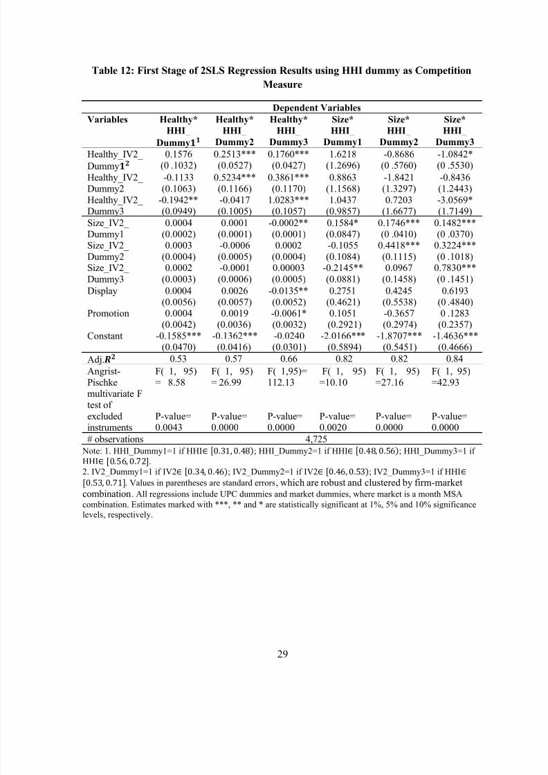
Table 12: First Stage of 2SLS Regression Results using HHI dummy as Competition

Measure

Dependent Variables

Variables Healthy*

HHI_Dummy

Healthy*

HHI_Dummy2

Healthy*

HHI_Dummy3

Size*

HHI_Dummy1

Size*

HHI_Dummy2

Size*

HHI_Dummy3

Healthy_IV2_

Dummy

0.1576(0 .1032)

0.2513***(0.0527)

0.1760***(0.0427)

1.6218(1.2696)

-0.8686(0 .5760)

-1.0842*(0 .5530)

Healthy_IV2_Dummy2

-0.1133(0.1063)

0.5234***(0.1166)

0.3861***(0.1170)

0.8863(1.1568)

-1.8421(1.3297)

-0.8436(1.2443)

Healthy_IV2_Dummy3

-0.1942**(0.0949)

-0.0417(0.1005)

1.0283***(0.1057)

1.0437(0.9857)

0.7203(1.6677)

-3.0569*(1.7149)

Size_IV2_Dummy1

0.0004(0.0002)

0.0001(0.0001)

-0.0002**(0.0001)

0.1584*(0.0847)

0.1746***(0 .0410)

0.1482***(0 .0370)

Size_IV2_

Dummy2

0.0003

(0.0004)

-0.0006

(0.0005)

0.0002

(0.0004)

-0.1055

(0.1084)

0.4418***

(0.1115)

0.3224***

(0 .1018)

Size_IV2_Dummy3 0.0002(0.0003) -0.0001(0.0006) 0.00003(0.0005) -0.2145**(0.0881) 0.0967(0.1458) 0.7830***(0 .1451)

Display 0.0004 0.0026 -0.0135** 0.2751 0.4245 0.6193(0.0056) (0.0057) (0.0052) (0.4621) (0.5538) (0 .4840)

Promotion 0.0004 0.0019 -0.0061* 0.1051 -0.3657 0 .1283(0.0042) (0.0036) (0.0032) (0.2921) (0.2974) (0.2357)

Constant -0.1585*** -0.1362*** -0.0240 -2.0166*** -1.8707*** -1.4636***(0.0470) (0.0416) (0.0301) (0.5894) (0.5451) (0.4666)

Adj. 0.53 0.57 0.66 0.82 0.82 0.84

Angrist-Pischkemultivariate F

test of

F( 1, 95)= 8.58

F( 1, 95)= 26.99

F( 1,95)=112.13

F( 1, 95)=10.10

F( 1, 95)=27.16

F( 1, 95)=42.93

excludedinstruments

P-value=0.0043

P-value=0.0000

P-value=0.0000

P-value=0.0020

P-value=0.0000

P-value=0.0000


Note: 1. HHI_Dummy1=1 if HHI [ ); HHI_Dummy2=1 if HHI [ ); HHI_Dummy3=1 if

HHI [ .2. IV2_Dummy1=1 if IV2 [ ); IV2_Dummy2=1 if IV2 [ ); IV2_Dummy3=1 if HHI

[ . Values in parentheses are standard errors, which are robust and clustered by firm-marketcombination. All regressions include UPC dummies and market dummies, where market is a month MSA

combination. Estimates marked with ***, ** and * are statistically significant at 1%, 5% and 10% significance

levels, respectively.



Table 13: UPC Regression Results using HHI dummy as Competition Measure

Dependent Variables

UPC dummy

Coefficients

from OLS

regressions for

price

UPC dummy

Coefficients

from IV

regressions for

price

UPC dummy

Coefficients

from OLS

regressions for

log price

UPC dummy

Coefficients

from IV

regressions for

log price

Healthy 0.9452*** 2.0217*** 0.0355 0.0878***(0.2587) (0.2600) (0.0294) (0.0294)

Size -0.0246*** -0.0279*** -0.0033*** -0.0039***(0.0026) (0.0027) (0.0003) (0.0003)

Constant -1.9470** -2.0010** -0.0382 -0.0378

(0.8315) (0. 8356) (0.0947) (0.0946)

Adj. 0.93 0.96 0.82 0.89

# observations 238

Note: Values in parentheses are standard errors. All regressions include firm dummy variables. Estimates


Market Competition and Price Discrimination the Case of Ketchup

Documents

Transcript of Market Competition and Price Discrimination the Case of Ketchup