Contents lists available at ScienceDirect

Marine Pollution Bulletin

journal homepage: www.elsevier.com/locate/marpolbul

Baseline

Remote sensing and water quality indicators in the Korean West coast:Spatio-temporal structures of MODIS-derived chlorophyll-a and totalsuspended solids

Hae-Cheol Kima, Seunghyun Sonb, Yong Hoon Kimc, Jong Seong Khimd, Jungho Name,Won Keun Change, Jung-Ho Leef, Chang-Hee Leeg,⁎, Jongseong Ryuf,⁎⁎

a I.M. Systems Group at NOAA/NWS/NCEP, Rockville, MD, USAb CIRA at NOAA/NESDIS/STAR, Fort Collins, CO, USAc Department of Earth and Space Sciences, West Chester University of Pennsylvania, West Chester, PA, USAd School of Earth and Environmental Sciences & Research Institute of Oceanography, Seoul National University, Seoul, Republic of Koreae Korea Maritime Institute, Pusan, Republic of Koreaf Department of Marine Biotechnology, Anyang University, Ganghwa-gun, Incheon, Republic of Koreag Department of Environmental Engineering and Energy, Myongji University, Yongin, Republic of Korea

A R T I C L E I N F O

Keywords:Chlorophyll-aSuspended solidsSurface temperatureRemote sensingYellow Sea

A B S T R A C T

The Yellow Sea is a shallow marginal sea with a large tidal range. In this study, ten areas located along thewestern coast of the Korean Peninsula are investigated with respect to remotely sensed water quality indicatorsderived from NASA MODIS aboard of the satellite Aqua. We found that there was a strong seasonal trend withspatial heterogeneity. In specific, a strong six-month phase-lag was found between chlorophyll-a and totalsuspended solid owing to their inversed seasonality, which could be explained by different dynamics and en-vironmental settings. Chlorophyll-a concentration seemed to be dominantly influenced by temperature, whiletotal suspended solid was largely governed by local tidal forcing and bottom topography. This study demon-strated the potential and applicability of satellite products in coastal management, and highlighted find thatremote-sensing would be a promising tool in resolving orthogonality of large spatio-temporal scale variabilitieswhen combining with proper time series analyses.

Coastal environments throughout the world are now experiencingunprecedented anthropogenic eutrophication, hypoxia and harmfulalgal blooms due to increased human activities and subsequently in-creased nutrient loadings (Anderson et al., 2002; Diaz and Rosenberg,2008). Because of their significant role in human well-being relyingupon them, deterioration of water quality indicators (e.g., water tem-perature, dissolved oxygen, chlorophyll, inorganic nutrients, heavymetals, total suspended solid) can be potentially catastrophic formarine ecosystems as species are threatened by conditions which are nolonger suitable for their survival (Bierman et al., 2011). As a result,monitoring changes in spatio-temporal patterns of water quality (WQ)in both terrestrial and marine ecosystems, and interpretation of theimplications have been important across disciplines these days, such asenvironmental/marine sciences and socio-economics. However, it isinherently difficult to properly address varying spatial and temporalscales of WQ for application to coastal marine waters monitoring and

assessment (Bierman et al., 2011).Recently, the application of satellite and airborne remote sensing

imagery to collect WQ information has become more frequent (Goetzet al., 2008). Remotely sensed datasets are generally more compre-hensive than those directly measured in situ in that they provide greaterspatial coverage with finer resolution and often increased temporalfrequency and resolution. This makes remote-sensing approach a richsource of data. However, the large amount of data also embeds chal-lenges for the extraction of meaningful information of WQ parameters.Remotely-sensed sea surface temperature (SST) is one of the most im-portant oceanic and atmospheric variables which has been widely usedin a variety of researches to develop an understanding of ocean dy-namics, as well as physical and biogeochemical processes in the upperocean (Park et al., 2015). For example, the year-to-year variations ofSST in the Yellow Sea (YS) may significantly affect the Korean, Chineseand Japanese climate, and thus it is important to examine the

http://dx.doi.org/10.1016/j.marpolbul.2017.05.026Received 11 December 2016; Received in revised form 9 May 2017; Accepted 11 May 2017

⁎ Correspondence to: C.H. Lee, Department of Environmental Engineering and Energy, Myongji University, Yongin, Gyeonggi-do 449-728, Republic of Korea.⁎⁎ Correspondence to: J. Ryu, Department of Marine Biotechnology, Anyang University, Ganghwa, Incheon 417-833, Republic of Korea.E-mail addresses: changhee@mju.ac.kr (C.-H. Lee), jsryu@anyang.ac.kr (J. Ryu).

Marine Pollution Bulletin 121 (2017) 425–434

Available online 20 June 20170025-326X/ © 2017 Elsevier Ltd. All rights reserved.

MARK

characteristic variability of SST, which may help assess the climatevariability and its down-scaled impacts over the YS and adjacentcountries (Yeh and Kim, 2010).

The global distribution of chlorophyll-a (Chl-a), the direct proxy forphytoplankton biomass (Cullen, 1982), shows Chl-a rich regions locatedalong the coasts and continental shelves, mostly because of a strongnutrient supply from continents. The visualization of satellite images isthe primary technique used to identify their presence, in particularwhen phytoplankton blooms occur as a regular event in a specific oceanregion (Srokosz and Quartly, 2013), or in regions where they are notusually expected such as oligotrophic gyres in North Pacific (Wilson,2003; Wilson et al., 2008). During the last decade, there has been anincrease in peer-reviewed publications on the study of algal bloomsusing ocean color satellite data (Blondeau-Patissier et al., 2014). Algalblooms in coastal ocean regions have mainly been the primary focus ofthose studies mostly because of the direct connectivity between landand coastal waters (Gazeau et al., 2004). Additionally, the second andthird generation development of satellite ocean color sensors allowedmore accurate retrieval of phytoplankton proxies in coastal waters(Shen et al., 2012).

Recent reviews on satellite ocean color remote sensing have re-ported on the scientific advances, societal benefits (IOCCG, 2008) andapplications to coastal ecosystem management (Kratzer et al., 2014;Klemas, 2011), including fisheries (Wilson, 2011) and harmful algalblooms detection (Shen et al., 2012). These ocean color datasets allowfor the derivation of ecological baselines which can then be used todetect and anticipate changes in the ocean systems' dynamics (Siegelet al., 2013; Wong et al., 2009; Smetacek and Cloern, 2008). Archivedearth observation data can be used in hindsight to assess prevailingbloom conditions and to identify biological and physical parametersthat triggered or terminated an algal event (Kahru et al., 1993).

In coastal waters, total suspended solid (TSS) can be an importantfactor controlling biological processes (Doxaran et al., 2003) and itsdistribution and variations can be strongly influenced by tides and riverdischarge (Stumpf and Pennock, 1989; Son et al., 2014; Kim et al.,2014). TSS is also important in light penetration and water movementsin the coastal waters (Son et al., 2014). Thus, accurate estimation of TSSis critical to understand the thermal structure of upper water columnsand physical processes (Lewis et al., 1990; Morel and Antoine, 1994;Sathyendranath et al., 1991) as well as biological processes (e.g.,phytoplankton photosynthesis) in the ocean euphotic zone (Platt et al.,1988; Sathyendranath et al., 1989).

There have been extensive studies on spatial and temporal dis-tribution of SST, Chl-a, and TSS both in the offshore and coastal regionsof the YS (Park and Oh, 2000; Xie et al., 2002; Ahn et al., 2004; Chuet al., 2005; Yeh and Kim, 2010; Wei et al., 2010; Lee et al., 2013; Sonet al., 2014; Park et al., 2015;). None of the studies, however, attempt toaddress these three components combined with respect to the inter-active dynamics between them, and few studies have compared WQdata derived from satellite with in situ monitoring data. The researchobjectives of this paper include: 1) examining spatial and temporalvariability of SST, Chl-a and TSS in the YS; 2) ground-truthing of sa-tellite data based on long-term monitoring data in situ, 3) presentingapplicability of satellite-based SST, Chl-a and TSS data with better de-scriptions of spatio-temporal patterns over larger areas of the YS to WQmanagement.

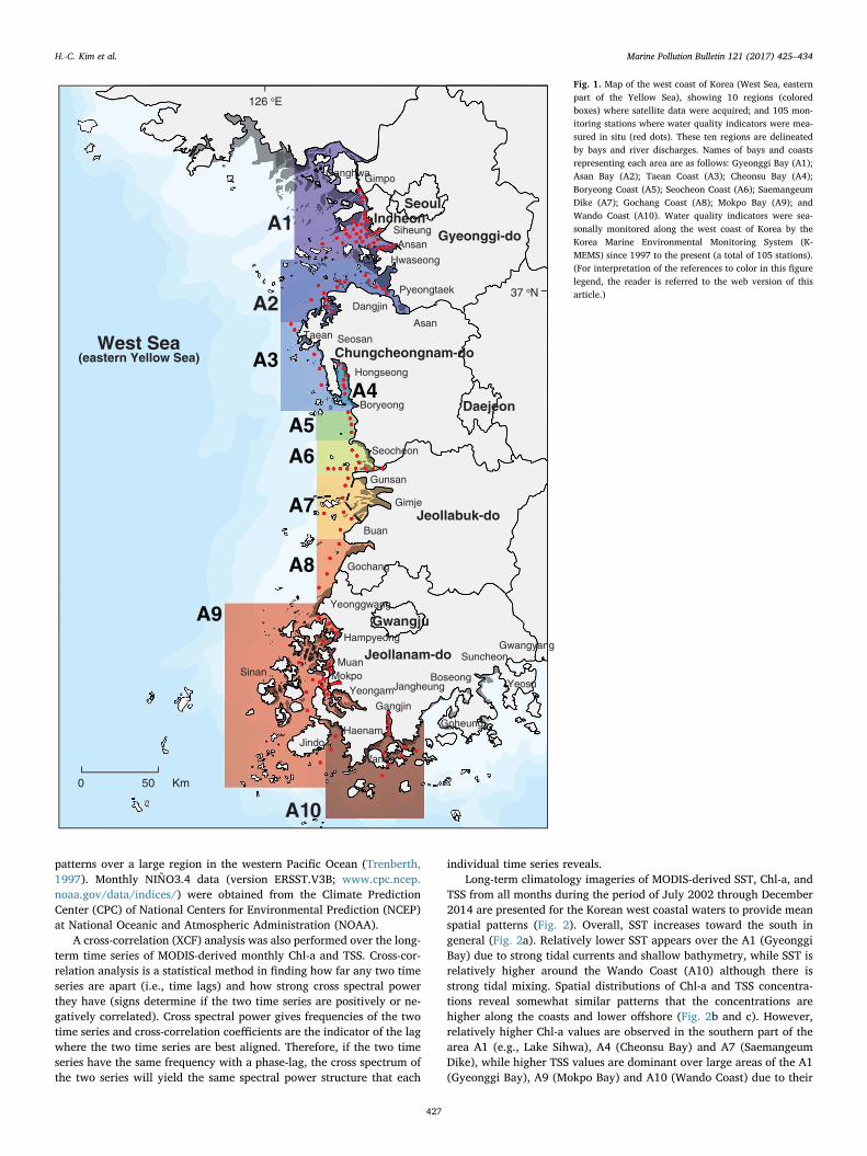
The Yellow Sea (YS) is a marginal sea with shallow depth (c.a. 44 m;Wei et al., 2010) and large tidal range reaching up to 10 m (Choi andKim, 2006). In the present study, 10 regions in Korean west coast(KWC), where satellite data were acquired, are delineated by bays andriver discharges as follows (Fig. 1): Gyeonggi Bay (A1); Asan Bay (A2);Taean Coast (A3); Cheonsu Bay (A4); Boryeong Coast (A5); SeocheonCoast (A6); Saemangeum Dike (A7); Gochang Coast (A8); Mokpo Bay(A9); and Wando Coast (A10). Geographical coordinates of delineatedboundaries of each are listed in Table S1.

To provide spatial distribution and temporal trends of WQ in the

study area, SST, Chl-a, TSS of surface waters were analyzed based onthe in situ data provided by Marine Environmental Monitoring Systemof Korea (K-MEMS). As for the purpose of regional comparison, 10 re-gions are allocated along KWC (Fig. 1). Han River estuary was set as anorthern limit and Wando Coast as a southern limit of the boundary. K-MEMS has been seasonally monitoring SST, Chl-a and TSS at a total of105 stations in the study area since 1997 to the present.

The ocean color and sea surface temperature data from the NASAModerate Resolution Imaging Spectroradiometer (MODIS) on the sa-tellite Aqua are available from the NASA's Ocean Color website (http://oceancolor.gsfc.nasa.gov/) supported by the Ocean Biology ProcessingGroup (OBPG) at NASA's Goddard Space Flight Center. MODIS-AquaLevel-2 daily ocean color products such as Chl-a and remote sensingreflectance (Rrs) at various wavelengths (Rrs(λ)), and day time SSTcovering the KWC waters (Fig. 1) were obtained from the NASA oceancolor website for the period of July 2002 to December 2014. TheMODIS-Aqua level-2 ocean color data were derived using the standardatmospheric correction algorithm with the near infrared (NIR) radiancecorrections (Bailey et al., 2010; Stumpf et al., 2003). The MODIS Chl-adata are derived using the NASA standard ocean color chlorophyll al-gorithm for MODIS (OC3M) (O'Reilly et al., 2000). The day time MODISSST product from the NASA OBPG are derived using the long-wave SSTalgorithm with MODIS bands at 11 and 12 μm (Minnett et al., 2004).More information about the MODIS-Aqua Level-2 data can be found atthe OBPG website (http://oceancolor.gsfc.nasa.gov/WIKI/OCReproc2013(2e)0MA.html). Those Level-2 data were remapped toa standard Mercator projection at 1 × 1 km spatial resolution for thestudy area.

The regional TSS model (Siswanto et al., 2011; Son et al., 2014)using Rrs at 3 wavelengths (488, 547, and 667 nm) were applied to theremapped daily MODIS-Aqua data to generate TSS maps in KWC asfollows:

= + ⋅ + − ⋅Log TSS R R RR

( ) 0.649 25.623 [ (555) (670)] 0.646 (490)(555)rs rs

rs

rs

(1)

Monthly and climatology monthly composite SST, Chl-a, and TSSimages were generated using the daily MODIS-derived products tocharacterize spatial and temporal variation of SST, Chl-a, and TSS in theYellow and East China Seas. Time series of a long-term climatology(mean distribution of all months from July 2002 to December 2014)and monthly climatological images (12-year mean for each month) ofSST, Chl-a and TSS from the MODIS-Aqua data were generated for the10 study regions (Fig. 1 and Table S1).

In this study, authors used MODIS-derived data set from the 10regions to decompose into principal components to examine spatio-temporal structure of Chl-a and TSS. In general, empirical orthogonalfunction (EOF) is used to analyze spatial structure by decomposing ofspatial multivariate data. EOF analysis is a principal component ana-lysis (PCA) applied to a group of time series over a certain spatial range,such as multiple points or 2-D field data sets. A new time series of co-herent variations (a.k.a., scores) was created from original time seriesand eigenvectors of covariance matrix (a.k.a., loadings) from EOFanalysis. The time series of coherent variation for the major principalcomponent (PC1 or EOF mode 1 explaining temporal pattern) was thenfiltered removing seasonality in order to focus on inter-annual varia-bility and was compared using cross-spectral analysis to compute lagsbetween the two time series.

After seasonality removed, filtered time series of coherent variation(i.e., scores) for the major principal component (PC1 or EOF mode 1)from Chl-a time series was compared against NIÑO3.4, which is a re-presentative climate index for one of El Niño Southern Oscillation(ENSO) indices. The NIÑO3.4 is defined by mean SST over the region of5° S–5° N and 170° W–120° W. It has been reported that this is a regionof great climate variability in ENSO time scale and has proximity to thearea where there is important effect in shifted SST on the precipitation

H.-C. Kim et al. Marine Pollution Bulletin 121 (2017) 425–434

426

patterns over a large region in the western Pacific Ocean (Trenberth,1997). Monthly NIÑO3.4 data (version ERSST.V3B; www.cpc.ncep.noaa.gov/data/indices/) were obtained from the Climate PredictionCenter (CPC) of National Centers for Environmental Prediction (NCEP)at National Oceanic and Atmospheric Administration (NOAA).

A cross-correlation (XCF) analysis was also performed over the long-term time series of MODIS-derived monthly Chl-a and TSS. Cross-cor-relation analysis is a statistical method in finding how far any two timeseries are apart (i.e., time lags) and how strong cross spectral powerthey have (signs determine if the two time series are positively or ne-gatively correlated). Cross spectral power gives frequencies of the twotime series and cross-correlation coefficients are the indicator of the lagwhere the two time series are best aligned. Therefore, if the two timeseries have the same frequency with a phase-lag, the cross spectrum ofthe two series will yield the same spectral power structure that each

individual time series reveals.Long-term climatology imageries of MODIS-derived SST, Chl-a, and

TSS from all months during the period of July 2002 through December2014 are presented for the Korean west coastal waters to provide meanspatial patterns (Fig. 2). Overall, SST increases toward the south ingeneral (Fig. 2a). Relatively lower SST appears over the A1 (GyeonggiBay) due to strong tidal currents and shallow bathymetry, while SST isrelatively higher around the Wando Coast (A10) although there isstrong tidal mixing. Spatial distributions of Chl-a and TSS concentra-tions reveal somewhat similar patterns that the concentrations arehigher along the coasts and lower offshore (Fig. 2b and c). However,relatively higher Chl-a values are observed in the southern part of thearea A1 (e.g., Lake Sihwa), A4 (Cheonsu Bay) and A7 (SaemangeumDike), while higher TSS values are dominant over large areas of the A1(Gyeonggi Bay), A9 (Mokpo Bay) and A10 (Wando Coast) due to their

A10

A2

A9

A3

A7

A6

A1

A5

Seoul

Gyeonggi-do

Chungcheongnam-do

Jeollabuk-do

Jeollanam-do

Gwangju

Incheon

Daejeon

Gimpo

SiheungAnsan

Hwaseong

Pyeongtaek

Asan

Dangjin

SeosanTaean

Hongseong

Boryeong

Seocheon

Gunsan

Gimje

Buan

Gochang

Yeonggwang

Hampyeong

MuanSinan

JindoHaenam

Yeongam

Gangjin

JangheungBoseong

Goheung

Suncheon

Yeosu

Gwangyang

Wando

Mokpo

West Sea(eastern Yellow Sea)

0 50 Km

126 oE

37 oN

Ganghwa

A8

A4

Fig. 1. Map of the west coast of Korea (West Sea, easternpart of the Yellow Sea), showing 10 regions (coloredboxes) where satellite data were acquired; and 105 mon-itoring stations where water quality indicators were mea-sured in situ (red dots). These ten regions are delineatedby bays and river discharges. Names of bays and coastsrepresenting each area are as follows: Gyeonggi Bay (A1);Asan Bay (A2); Taean Coast (A3); Cheonsu Bay (A4);Boryeong Coast (A5); Seocheon Coast (A6); SaemangeumDike (A7); Gochang Coast (A8); Mokpo Bay (A9); andWando Coast (A10). Water quality indicators were sea-sonally monitored along the west coast of Korea by theKorea Marine Environmental Monitoring System (K-MEMS) since 1997 to the present (a total of 105 stations).(For interpretation of the references to color in this figurelegend, the reader is referred to the web version of thisarticle.)

H.-C. Kim et al. Marine Pollution Bulletin 121 (2017) 425–434

427

local characteristics, such as shallow bathymetry and strong tidalmixing.

Monthly climatological (2002−2012) images of MODIS-derivedSST, Chl-a, and TSS for the KWC are derived (Fig. 3). In general, spatialdistributions of the climatological monthly SST, Chl-a, and TSS imagesare similar to that from the climatology images from July 2002 toDecember 2014 shown in Fig. 2, and there are strong seasonal vari-abilities over the entire study areas.

The MODIS-derived SST images show that SST is lower in thecoastal waters (lowest in Gyeonggi Bay) while SST is higher offshorewaters and southern YS over all months (Fig. 3a). The lower SST alongthe coasts, especially in Gyeonggi (A1) and Wando Coast (A10) area, iscaused by strong vertical mixing due to the tidal currents and shallowbathymetry. Lower SST appears in winter months (with lowest inFebruary with mean SST by about 2 °C in A1) and higher SST in summermonths (highest in August with mean SST by about 28 °C in the entireKWC).

Monthly climatology of the MODIS imageries provides that Chl-aconcentrations are higher onshore of the KWC and lower in the middleand south offshore of the YS in most of months (Fig. 3b). However, inthe middle of the YS, Chl-a concentrations are higher in spring months(March to May) and autumn (November to December). The highest Chl-

a values in April would be related to spring phytoplankton bloom in themiddle of the YS. The lowest Chl-a values appear during the summermonths in the middle of YS. However, relatively higher Chl-a con-centrations are shown in summer season along the KWC (e.g., highestSST values in August from A4 and A7).

General spatial distributions of the MODIS-derived monthly TSSreveal similar patterns to those long-term climatological TSS from 2002to 2014, showing higher TSS along the KWC (especially, in A1 ofGyeonggi Bay and A10 of Wando Coast area) and lower in offshore(minimum in the middle of the YS) (Fig. 3c). The TSS values are highestin winter (December to March) and lowest in summer months (July toAugust) in all regions. The maximum TSS values are shown in A1(Gyeonggi Bay) and A10 (Wando Coast) region (about 10–12 mg L−1

on average) in the winter months. The ribbon-shaped features are al-ways shown in A1 over all months, which is attributed to the tidalasymmetry effect (Jay and Musiak, 1994) because Gyeonggi Bay isunder estuarine regime where fresh- and salt-water mixing occurs moreactively than other 9 regions (Son et al., 2014).

This section describes the temporal variability of SST, Chl-a, andTSS in each region for the past 10 years (2004–2014), by analyzingboth satellite-derived and in situ observation data. Fig. 4a shows thetime series of SST in 10 regions. Red circles represent the data

SST)c(a-lhC)b(TSS)a(

SSTa-lhCTSS (°C) (µg chl-a / l)

0 8.0 16.0 24.0 32.0 0.1 1.0 10.0 64.0 0.05 0.10 1.00 10.00 25.00

(mg / l)

Fig. 2. MODIS-derived long-term climatology images in the west coast of Korea (July 2002-Dec 2014). (a) sea surface temperature (SST), (b) chlorophyll-a (Chl-a), and (c) totalsuspended solids (TSS) of surface waters.

H.-C. Kim et al. Marine Pollution Bulletin 121 (2017) 425–434

428

seasonally observed in situ observed, while the blue lines are for theMODIS-derived monthly SST. The most striking feature is the seasonalvariability of SST, whereby warm during summer and cold duringwinter. In general, MODIS-derived SST matches very well with theobservation data particularly in northern regions (e.g., A1–A6). In thesouthern areas (e.g., A7–A10), the MODIS-derived values tend toslightly overestimate the SST especially during winter, but the dis-crepancies are not noticeable.

Time-series of Chl-a for each region is plotted in Fig. 4b. Whencompared to SST, one can note that the discrepancy between the ob-servation and MODIS-derived Chl-a concentrations which are two orthree times larger in magnitude than the in situ measurements. Overall,the observation data range 0 to 5 μg L−1 for most periods other thansome spikes. Those spikes occur early spring (February or March) in A1and A2, which thought to represent early-spring blooming in the coastalareas (Fig. 4a and b). Some exceptional cases of these spikes occurringduring summer months in A3–A8 can be found in both observation andMODIS-derived data during 2005–2007 (Fig. 4b). Chl-a concentrationin A4 (Cheonsu Bay) shows the highest values out of all 10 regions,which are consistent in both observation and MODIS-derived data.Some of spikes are coherent among regions, but hard to find the trendin spatial coherency. MODIS-derived data overestimate in situ Chl-aexcept for regions of A9 and A10.

Fig. 4c depicts the temporal variability of TSS in 10 regions. Similarto the case of Chl-a, there exists discrepancy between in situ measure-ments and MODIS-derived TSS. In general, the MODIS-derived TSS issmaller than the in situ measurements with little exception, contrary toChl-a cases.

An empirical orthogonal function (EOF) analysis (a.k.a., principalcomponent analysis: PCA) is applied to the long-term time series of

MODIS-derived monthly Chl-a and TSS data from 10 regions (Figs. 5, 6and 7). As mentioned earlier, a PCA is a statistical tool to decomposemultiple variables into principal components having orthogonality, andthese components can be ranked with respect to its contribution thatcan explain variances of the time series. Eigenvectors of the co-variancematrix from the MODIS-derived Chl-a and TSS at 10 regions are plottedin 2-dimensional X–Y space with X being PC1 and Y being PC2 (Fig. 5aand b), respectively. Variance explained by 10 PCs for the same timeseries data sets are also presented.

It is noteworthy that loadings from both Chl-a and TSS times seriesare located on the positive axis of PC1 (upper right and lower rightquadrant) which represents temporal structure (Fig. 5a and b). Thisindicates that all 10 regions have similar and strong seasonal patterns ofChl-a and TSS and their variances can be significantly explained by PC1(47.3% and 74.6%, respectively). However, PC2, representing spatialstructure, reveals somewhat different features than PC1 has shown.Loadings from each region are clustered into two groups along the PC2axis (see colored circles grouping 10 regions into two in Fig. 5a and b).Bays from the northern part of the YS (A1 and A2) are grouped togetherwith those from the south (A9 and A10) in the positive axis of the PC2(upper right quadrant) for Chl-a (Fig. 5a) and negative axis of the PC2(lower right quadrant) for TSS time series (Fig. 5b), respectively. Thisindicates that Chl-a and TSS behaviors in the north (A1 and A2) andsouth (A9 and A10) are different from the rest regions (A3–A7, e.g.,Saemangeum Dike and Cheonsu Bay). This synoptic heterogeneity waspreviously described in the monthly climatological characteristics.

To determine time lags between the two time series, a cross-corre-lation function (XCF) is applied to the long-term time series of MODIS-derived monthly Chl-a and TSS. Fig. 6 presents PC1 (EOF mode 1) fromChl-a time series overlaid by that from the TSS time series. It was found

Jan

(a)SST

SST

(b)Chl-a

Chl-a

(c)TSS

TSS

Feb Mar Apr May Jun Jul Aug Sep Oct Nov Dec

0 8.0 16.0 24.0 32.0

(°C)

64.010.01.00.1

(µg chl-a / l)

25.0010.001.000.100.05

(mg / l)

Fig. 3. MODIS-derived monthly climatological images in the west coast of Korea (12-year mean for each month, July 2002-Dec 2014). (a) sea surface temperature (SST), (b) chlorophyll-a(Chl-a), and (c) total suspended solids (TSS) of surface waters.

H.-C. Kim et al. Marine Pollution Bulletin 121 (2017) 425–434

429

that there is a strongly negative correlation in the PC1 (EOF mode 1)from the two time series (Fig. 6a). This was statistically supported bystrongly negative cross spectral power at the frequency of 1 year(Fig. 6b) indicating that both Chl-a and TSS time series have 1-yearfrequency but their peaks are negatively correlated. The coherence ofthe 1-year frequency is about 0.85 which was found to be statisticallysignificant (p < 0.05) within 95% confidence level (Fig. 6c). In thisXCF analysis, even if not statistically significant, it was found that thereis a 6-month phase-lag between the two PC1 of Chl-a and TSS timeseries data and the correlation coefficient of this phase-shift is 51%(Fig. 6d). This negative correlation between the two properties was alsoshown in the PCA data structure in Fig. 5. One can note that these twogroups (north and south regions vs. middle regions) reveal inversedrelationship between the Chl-a and TSS time series. For example, thoseregions with positive PC2 (upper right quadrant) of Chl-a are located inthe negative side of PC2 (lower right quadrant) in TSS, and on thecontrary, those regions with negative PC2 (lower right quadrant) ofChl-a are located in the positive side of PC2 (upper right quadrant) inTSS. This finding is an interesting feature and will be discussed later.

It is noted that the MODIS-derived Chl-a concentrations would beoverestimated in the coastal waters due to non-algal components suchas colored dissolved organic matters (CDOM) and suspended sediments(SS) since the Chl-a algorithm (OC3) for the MODIS data works well forthe clear open ocean waters. The YS belongs to the marginal seas with“Case 2” optical complexities although central area of the YS is char-acterized as “Case 1” water during the summer months (Yoo and Park,1998), which was also confirmed by the present study (Fig. 3b). This“Case 2” water characteristics may be due to the large volume of

freshwater discharge from Yangtze and Han Rivers (Shen et al., 1998;Lee et al., 2013), and to strong tidal mixing and shallow bathymetry incoastal regions of the YS (Ahn et al., 2004). It is also due, in part, to thebifurcation of the Kuroshio Current and its complicated physicalproperties transporting suspended materials into the YS (Lie et al.,1998, 2001; Tseng et al., 2000; Lie and Cho, 2002; Ichikawa andBeardsley, 2002; Chu et al., 2005).

Despite the fact that TSS adds optical complexities to ocean colorretrieval (Chl-a) and that both Chl-a and TSS concentrations are, ingeneral, found to be high along the KWC, there are some spatial pat-terns that can distinguish Chl-a departure from TSS images in the KWC.While TSS is significantly higher in the A9 (Mokpo Bay) and A10(Wando Coast), Chl-a is relatively lower than other KWC regions byexamining seasonal Chl-a climatology patterns (Fig. 3b). In specific, thisdecoupling was pronounced during the plant growing season (April andMay). Region A9 and A10 show low Chl-a concentration even whenthere are offshore (middle of the YS) blooms occur in April (Fig. 3b),and TSS climatology still reveals higher concentration during the samemonths in those regions (Fig. 3c).

On the contrary, regions located in the middle part of the KWC (e.g.,A3–A6), Chl-a concentrations are relatively higher during April throughSeptember (see Fig. 3b), but TSS values are relatively lower comparedto adjacent regions (e.g., A1, A2, A9 and A10) for the same months(Fig. 3c). The same feature was found in in situ measurements collectedfrom A4–A6 regions during 2005–2007 (Fig. 4b). This indicates thatdespite the algorithmic limitation of “Case 1” ocean color product whenapplied to “Case 2” waters, the spatial distribution of MODIS-derivedChl-a in the KWC gives synoptic information about regional trends and

A1

A2

A3

A4

A5

A6

A7

A8

A9

SST)c(a-lhC)b(TSS)a(

A10

Fig. 4. Eleven-year time series data sets of (a) sea surface temperature (SST), (b) chlorophyll-a (Chl-a), and (c) total suspended solids (TSS) in 10 regions (A1–A10). Solid red lines withsquare symbols represent quarterly in situ measurements from K-MEMS stations, and solid blue lines represent MODIS-derived monthly data. (For interpretation of the references to colorin this figure legend, the reader is referred to the web version of this article.)

H.-C. Kim et al. Marine Pollution Bulletin 121 (2017) 425–434

430

patterns over larger areas and longer time periods, without necessarilyhaving too much bias due to coastal TSS. However, authors shouldpoint out that it is not clear whether discrepancies between satellite-derived data and in situ measurements are due to optical algorithms inthe turbid waters or due to mismatches of sampling period (monthlyand quarterly) and spatial averaging. Until this question is resolved,

these apparent differences will limit the quantitative usefulness of thisapproach to informing ecosystem managers. Continued efforts ofcoastal optical calibration/validation surveys are necessary in order tomore accurately and quantitatively partition each water quality con-stituents (e.g., Chl-a, TSS, CDOM) from the optically complex coastalwaters.

(d)(c)

(b)(a)Fig. 5. Biplots of MODIS-derived (a) chlorophyll-a (Chl-a) and (b) total suspended solids (TSS) from 10 regions.Circles represent two groups of regions revealing spatialheterogeneity along the principal component (PC) 2 axis.Variance explained by 10 PCs are presented for (c) Chl-aand (d) TSS. PC1 and 2 represent temporal and spatialdecomposition of the original time series data. Thestrongest explanation power that PC 1 has is 47.3% (Chl-a) and 74.6% (TSS).

Fig. 6. Time series analysis of chlorophyll-a (Chl-a) andtotal suspended solids (TSS) derived monthly from MODIS(July 2002–Dec 2014). (a) Principal component 1 (EOFmode 1) of Chl-a time series overlaid by that of TSS timeseries. (b) Cross spectral power, (c) coherence and (d) crosscorrelation coefficients for time lags are presented.Horizontal dashed lines in grey and black color in (c) and(d) represent upper (95%) and lower (90%) limits of con-fidence interval, respectively. The vertical dashed line in(d) represents the point where the two time series have nophase-shift (zero phase-shift).

H.-C. Kim et al. Marine Pollution Bulletin 121 (2017) 425–434

431

As previously described, the MODIS-derived TSS show strong sea-sonality of higher values during winter and lower values duringsummer. However, this seasonality pattern is not clear in the in situmeasurements from K-MEMS (Fig. 4c). This could be attributed to thespatial heterogeneity of TSS, where high concentration of sediment mayoccur as patchy and point observation data may not be representativefor the region. It is hard to find correlation among regions, which in-dicates that the processes controlling TSS could be local rather thanregional. TSS is strongly affected by resuspension and physical pro-cesses, such as wind-induced winnowing, tidal currents and bottomtopography, which makes it difficult to accurately estimate TSS con-centration remotely from the space (Kang et al., 2009; Choi et al.,2012). In addition, increased human activities, such as coastal landcover/land use changes and coastal engineering projects, add morecomplexities in the coastal physical processes and dynamics of waterquality indicators (Choi et al., 2012; Jung and Kim, 2005). Recently,there have been studies on diurnal features of TSS changes in the KWS,YS and East China Sea using Geostationary Ocean Color Imager (GOCI)sensor (Kim et al., 2014; Son et al., 2014) to investigate physics-induced(mostly, tides and topography) hour-to-hour variations of TSS. How-ever, it should be noted that neither MODIS-derived TSS nor K-MEMS insitu measurements in this study reflect high temporal frequency (hourlytime scale) signatures. Thus, satellite-derived TSS data and resultspresented here are more suitable for analyzing the regional andmonthly climatological characteristics of suspended sediment dis-tribution in the KWS. Son et al. (2014) investigated temporal variationsin TSS concentration in the turbid coastal waters (including GyeonggiBay and Wando Coast), and also suggested that the satellite approachescan be applicable to synoptic studies of sediment dynamics in theseareas influenced by strong tidal current.

Fig. 5 reveals that almost all the PC1's from the MODIS-derived Chl-a and TSS at the study regions (except for A9) in the KWC are located onthe positive side of PC1 axis, which implies that all the regions havevery similar temporal structure, while there exists spatial heterogeneityin the two time series indicated by two clusters along the PC2 axis.Although having almost the same temporal structure mentioned above,

it is notable that the distribution of Chl-a along the PC1 shows a morewidely spread pattern than that of TSS which has a more or less nar-rowly aligned pattern along the PC1. In fact, biplot structure of TSSresembles that of SST (not shown in Fig. 5), which indicates that TSSconcentration is more or like a quasi-conservative tracer (i.e., de-pending on seasonality); whereas, Chl-a shows a non-conservativeproperty having intrinsic biological processes governing local growthand loss of phytoplankton biomass. Besides differences in the intrinsicrate, another possible explanation may include resuspension-inducedTSS dynamics. Wynne et al. (2006) reported that inorganic sedimentcontributes up to 94% of total resuspended materials in the Texascoasts, while resuspended benthic algae is 6%. This may indirectlyexplain why TSS, as a quasi-conservative tracer, strongly influenced byphysical processes revealed similar structure to SST in eigenvectors ofcovariance matrices (i.e., loadings).

Then what caused spatial heterogeneity in both Chl-a and TSS timeseries? Choi et al. (2003) found that relatively low primary productionis found near Gyeonggi Bay (A1) and the southwestern KWC (A9 andA10), while central waters of the YS is productive during the fieldcampaign in 1997 (February, April, August, October and December). Inaddition, high Chl-a concentration was found near the Taean coastalarea (A3) and Cheonsu Bay (A4) where there was tidal front extendedfrom the offshore (Choi, 1987; Seung et al., 1990; Choi et al., 1995).Similar spatial pattern was found in the monthly climatology of MODIS-derived Chl-a as previously mentioned (Fig. 3b). In general, chlorophylldynamics in the coastal zones is influenced by temperature for growth,nutrients loadings, species composition (size fraction) of phyto-plankton, light condition, and mixing/stratification. The YS and KWChave many complexities with respect to land-sea hydrology, tidal in-fluences, seasonal bottom cold water mass and current features asso-ciated with Kuroshio bifurcations (Lie, 1986; Choi, 1987; Seung et al.,1990; Choi et al., 1995).

Tidal currents-induced resuspension and transport are dominatingprocesses in TSS dynamics (Lee et al., 2013; Son et al., 2014). Diurnal(hour-to-hour) variations in TSS assessed with GOCI clearly demon-strated that TSS dynamics in Gyeonggi Bay (near A1 and A2) and

Fig. 7. Time series analysis of monthly chlorophyll-a (Chl-a) derived from MODIS (July 2002–Dec 2014). (a) Principalcomponent 1 (EOF mode 1) of Chl-a time series overlaid byNIÑO3.4 index. Positive index represents warm years whenEl Niño mode happens and negative index represents coldyears when La Niña mode happens. (b) Cross spectralpower, (c) coherence and (d) cross correlation coefficientsfor time lags are presented. Horizontal dashed lines in greyand black color in (c) and (d) represent upper (95%) andlower (90%) limits of confidence interval, respectively. Thevertical dashed line in (d) represents the point where thetwo time series have no phase-shift (zero phase-shift).

H.-C. Kim et al. Marine Pollution Bulletin 121 (2017) 425–434

432

Wando Coast (near A9 and A10) is strongly influenced by tidal currents,e.g., tidal asymmetry effect in stratification (see the discussion in Sonet al., 2014), while other middle regions of the KWC (e.g., Taean Coast,Cheonsu Bay, Saemangeum Dike) do not seem to have as strong tidaleffects as Gyeonggi Bay and Wando Coast have because tidal influenceand topographical settings are different.

Although minor discrepancies exist between the two PC1's fromMODIS-derived Chl-a and TSS, both time series are found to have strongcross spectral power at the frequency of 1 year (Fig. 6b), which impliesthat there is a strong seasonality in both properties. Interestingly, thephase between the two is 6 months apart (Fig. 6a and d). This strongnegative cross correlation is presumed to be largely due to strong sea-sonal variabilities that YS environmental factors have. Son et al. (2014)reported that the sediment dynamics of the YS and East China Sea ischaracterized with strong seasonality, showing highest in winter andlowest in summer months. This seasonal pattern is related to manyfactors that also affect SST in the region, such as monsoon, advection,vertical mixing and bottom topography (Furey and Bower, 2005; Xieet al., 2002). In specific, basin scale atmospheric pressure system (i.e.,monsoon) and the bathymetry effects play a critical role in creatingthese seasonal trends because these two factors will change features ofwind-induced mixing (waves and surface currents), resuspension, andthus, TSS dynamics, consequently. Likewise, overall chlorophyll dy-namics in the coastal zones is strongly influenced by optimal tem-perature, nutrients and light availability for photosynthesis. Althoughcomplicated oceanographic conditions exist, phytoplankton growthgenerally occurs during spring, summer and fall season in the YS andKWC regions (Choi, 1987; Lie, 1986; Seung et al., 1990; Choi et al.,1995). Therefore, authors speculate that 6-month phase-lag betweenMODIS-derived Chl-a and TSS is largely due to strong inversed sea-sonality caused by different sets of drivers both properties have. It is notclear whether there is a certain connection in ecosystem dynamics be-tween the two properties.

So far, there have been few studies between year-to-year variationsof SST in the YS with basin-scale changes, such as linking to ENSO (Parkand Oh, 2000; Wu et al., 2005), although some researchers focused onlong-term warming trends of SST related to atmospheric patterns (Yehand Kim, 2010; Park et al., 2015). It has been believed that there is arather distinct teleconnection between changes in winter SST in the YSand ENSO. The present study found that there was a significant positivecross-correlation between the PC1 of SST measurements from K-MEMSand NIÑO3.4 index (not shown). Interestingly, the teleconnection of thePC1 from the Chl-a time series with NIÑO3.4 differed from the aboveSST case. Fig. 7 presents PC1 (EOF mode 1) from chlorophyll time seriesoverlaid by NIÑO3.4 index that is a representative climate index forENSO. Positive index represents warmer than normal (El Niño mode)and negative index represents colder than normal (La Niña mode), re-spectively. Although not significant, it is notable that there is slightnegative cross-correlation between the PC1 coefficients and NIÑO3.4(Fig. 7d), which was also found in K-MEMS measurements with dif-ferent time-lags (not shown). Authors speculate that this negative re-lationship may be related to ENSO-induced changes in terrestrial set-tings (e.g., quality and quantity of riverine discharges), changes in far-field physical processes (e.g., mixing patterns in the offshore of the YSand Kuroshio bifurcations, possibly), and/or changes in phytoplanktonphysiological responses or community structures. It certainly requiresfurther investigation in the future.

There are many eutrophication assessment frameworks: MarineStrategy Framework Directive in European Commission; AustralianNational Water Quality Management Strategy; Oslo Paris (OSPAR)Commission Common Procedure; Water Framework Directive (WFD) inEuropean Union; French Research Institute for Exploration of the Sea(IFREMER) method; Helsinki Commission (HELCOM) EutrophicationAssessment Tool; USA the National Coastal Assessment and NationalAquatic Resource Assessment (Park et al., 2010; Devlin et al., 2011;Ferreira et al., 2010; Dekker and Hestir, 2012). However, few

management decisions are made based on satellite-derived products(Schaeffer et al., 2013).

Good ecosystem-based coastal managements always require com-prehensive and quality-assured data and this requirement cannot befulfilled by only spatio-temporally limited, cost and labor intensive insitu monitoring data (Bierman et al., 2011). Remote sensing can pro-vide information embedding various spatio-temporal scales and com-plex dynamics of coastal processes (Schaeffer et al., 2013; Kratzer et al.,2014). For example, remote-sensing technique successfully monitoredtoxic cyanobacterial blooms in the Baltic Sea (Kahru et al., 2007;Kononen and Leppänen, 1997), Great Lakes and the eastern USA(Lunetta et al., 2015). Although this kind of success stories encouragesmanagement level to incorporate remotely sensing tool as a componentof integrated coastal zone management, it should be kept in mind thatsatellite technique cannot solve all the problems managers and policymakers may have, and that there are technical and logistic limitationsto be resolved (e.g, product accuracy, data continuity, programmaticsupport and cost issues discussed in Schaeffer et al., 2013).

In conclusion, MODIS-derived water quality indicators from theKorean west coast waters indicate that: 1) there is a strong seasonalityin decomposed principal components of SST, Chl-a and TSS time serieswith spatial heterogeneity between the north-south group (GyeonggiBay, Mokpo Bay, Wando Coast) and mid-coast group (Cheonsu Bay,Boryeong Coast, Saemangeum Dike); 2) there is a six-month phase-lagbetween Chl-a and TSS due to strongly inversed seasonality bothproperties have, which can be explained by different dynamics betweenthe two. Chl-a in the coastal zones is influenced by temperature forgrowth, while TSS is strongly influenced by tidal forcings and bottomtopography; 3) Chl-a may possibly be tele-connected with ENSO eventsnegatively. Remote-sensing technique can provide quantitative andsupplemental information and serve as an important decision sup-porting tool in coastal management.

Acknowledgements

This study was supported by the projects entitled “Integratedmanagement of marine environment and ecosystems aroundSaemangeum” (Grant No. 20140257) given to JR, JSK and JN and“Development of integrated estuarine management system” (Grant No.20140431) given to CHL, JR and JSK , both funded by the Ministry ofOceans and Fisheries, Republic of Korea.

Appendix A. Supplementary data

Supplementary data to this article can be found online at http://dx.doi.org/10.1016/j.marpolbul.2017.05.026.

References

Ahn, Y., Shanmugam, P., Gallegos, S., 2004. Evolution of suspended sediment patterns inthe East China and Yellow Seas. J. Korean Soc. Oceanogr. 39, 26–34.

Anderson, D.M., Glibert, P.M., Burkholder, J.M., 2002. Harmful algal blooms and eu-trophication: nutrient sources, composition, and consequences. Estuaries 25,704–726.

Bailey, S.W., Franz, B.A., Werdell, P.J., 2010. Estimation of near-infrared water-leavingreflectance for satellite ocean color data processing. Opt. Express 18, 7521–7527.

Bierman, P., Lewis, M., Ostendorf, B., Tanner, J., 2011. A review of methods for analysingspatial and temporal patterns in coastal water quality. Ecol. Indic. 11, 103–114.

Blondeau-Patissier, D., Gower, J.F., Dekker, A.G., Phinn, S.R., Brando, V.E., 2014. A re-view of ocean color remote sensing methods and statistical techniques for the de-tection, mapping and analysis of phytoplankton blooms in coastal and open oceans.Prog. Oceanogr. 123, 123–144.

Choi, J.-K., 1987. Influence of the shallow sea front off Kyeonggi Bay on primary pro-ductivity and community structure of phytoplankton. KOSEF Rep. 70 (in Korean).

Choi, K., Kim, S.-P., 2006. Late quaternary evolution of macrotidal Kimpo tidal flat,Kyonggi Bay, west coast of Korea. Mar. Geol. 232, 17–34.

Choi, J.-K., Noh, J.-H., Shin, K.-S., Hong, K.-H., 1995. The early autumn distribution ofchlorophyll-a and primary productivity in the Yellow Sea, 1992. The Yellow Sea 1,68–80.

Choi, J.-K., Noh, J.-H., Cho, S., 2003. Temporal and spatial variation of primary pro-duction in the Yellow Sea. Proc. Yellow Sea Int. Symp., Ansan South Korea 103–115.

H.-C. Kim et al. Marine Pollution Bulletin 121 (2017) 425–434

433

Choi, J.K., Park, Y.J., Ahn, J.H., Lim, H.S., Eom, J., Ryu, J.H., 2012. GOCI, the world'sfirst geostationary ocean color observation satellite, for the monitoring of temporalvariability in coastal water turbidity. J. Geophys. Res. Oceans 117.

Chu, P., Yuchun, C., Kuninaka, A., 2005. Seasonal variability of the Yellow Sea/EastChina Sea surface fluxes and thermohaline structure. Adv. Atmos. Sci. 22, 1–20.

Cullen, J.J., 1982. The deep chlorophyll maximum: comparing vertical profiles ofchlorophyll a. Can. J. Fish. Aquat. Sci. 39, 791–803.

Dekker, A., Hestir, E., 2012. Evaluating the Feasibility of Systematic Inland Water QualityMonitoring With Satellite Remote Sensing. Commonwealth Scientific and IndustrialResearch Organization (CSIRO), Canberra, Australia.

Devlin, M., Bricker, S., Painting, S., 2011. Comparison of five methods for assessing im-pacts of nutrient enrichment using estuarine case studies. Biogeochemistry 106,177–205.

Diaz, R.J., Rosenberg, R., 2008. Spreading dead zones and consequences for marineecosystems. Science 321, 926–929.

Doxaran, D., Froidefond, J.-M., Castaing, P., 2003. Remote-sensing reflectance of turbidsediment-dominated waters. Reduction of sediment type variations and changingillumination conditions effects by use of reflectance ratios. Appl. Opt. 42, 2623–2634.

Ferreira, J.G., Andersen, J., Borja, A., Bricker, S., Camp, J., Cardoso da Silva, M., Garcés,E., Heiskanen, A., Humborg, C., Ignatiades, L., 2010. Marine strategy frameworkdirective–task group 5 report eutrophication. EUR 24338, 49.

Furey, H.H., Bower, A.S., 2005. Synoptic temperature structure of the East China andsoutheastern Japan/East Seas. Deep-Sea. Res. PT. II. 52, 1421–1442.

Gazeau, F., Smith, S.V., Gentili, B., Frankignoulle, M., Gattuso, J.-P., 2004. The Europeancoastal zone: characterization and first assessment of ecosystem metabolism. Estuar.Coast. Shelf. S. 60, 673–694.

Goetz, S., Gardiner, N., Viers, J., 2008. Monitoring freshwater, estuarine and near-shorebenthic ecosystems with multi-sensor remote sensing: an introduction to the specialissue. Remote Sens. Environ. 112, 3993–3995.

Ichikawa, H., Beardsley, R.C., 2002. The current system in the Yellow and East Chinaseas. J. Oceanogr. 58, 77–92.

IOCCG, 2008. Why ocean colour? The societal benefits of ocean-colour technology. In:Platt, T. (Ed.), Reports of the International Ocean-Colour Coordinating Group.Bedford Institute, Dartmouth (Nova Scotia, Ca.).

Jay, D.A., Musiak, J.D., 1994. Particle trapping in estuarine tidal flows. J. Geophys. Res.Oceans 99, 20445–20461.

Jung, T.-S., Kim, S.-G., 2005. Monitoring system of coastal environment changes due tothe construction on the sea. J. Korean Soc. Mar. Environ. Energy 8, 53–59.

Kahru, M., Lepppaenen, J.-M., Rud, O., 1993. Cyanobacterial blooms heating of the seasurface. Mar. Ecol. Prog. Ser. 101, 1–7.

Kahru, M., Savchuk, O., Elmgren, R., 2007. Satellite measurements of cyanobacterialbloom frequency in the Baltic Sea: interannual and spatial variability. Mar. Ecol.Prog. Ser. 343, 15–23.

Kang, J.W., Moon, S.-R., Park, S.-J., Lee, K.-H., 2009. Analyzing sea level rise and tidecharacteristics change driven by coastal construction at Mokpo coastal zone in Korea.Ocean Eng. 36, 415–425.

Kim, Y.H., Im, J., Ha, H.K., Choi, J.-K., Ha, S., 2014. Machine learning approaches tocoastal water quality monitoring using GOCI satellite data. Gisci. Remote Sen. 51,158–174.

Klemas, V., 2011. Remote sensing techniques for studying coastal ecosystems: an over-view. J. Coast. Res. 27, 2–17.

Kononen, K., Leppänen, J., 1997. Patchiness, Scales and Controlling Mechanisms ofCyanobacterial Blooms in the Baltic Sea: Application of a Multiscale ResearchStrategy. Monitoring Algal Blooms: New Techniques for Detecting Large-scaleEnvironmental Change. Springer-Verlag, Heidelberg New York: Berlin, pp. 63–84.

Kratzer, S., Harvey, E.T., Philipson, P., 2014. The use of ocean color remote sensing inintegrated coastal zone management—a case study from Himmerfjärden, Sweden.Mar. Policy 43, 29–39.

Lee, H.J., Park, J.Y., Lee, S.H., Lee, J.M., Kim, T.K., 2013. Suspended sediment transportin a rock-bound, macrotidal estuary: Han estuary, Eastern Yellow Sea. J Coastal Res.29, 358–371.

Lewis, M.R., Carr, M.-E., Feldman, G.C., Esaias, W., McClain, C., 1990. Influence of pe-netrating solar radiation on the heat budget of the equatorial Pacific Ocean. Nature347, 543–545.

Lie, H.-J., 1986. Summertime hydrographic features in the southeastern Hwanghae. Prog.Oceanogr. 17, 229–242.

Lie, H.J., Cho, C.H., 2002. Recent advances in understanding the circulation and hy-drography of the East China Sea. Fish. Oceanogr. 11, 318–328.

Lie, H.J., Cho, C.H., Lee, J.H., Niiler, P., Hu, J.H., 1998. Separation of the Kuroshio waterand its penetration onto the continental shelf west of Kyushu. J. Geophys. Res.Oceans 103, 2963–2976.

Lie, H.J., Cho, C.H., Lee, J.H., Lee, S., Tang, Y., Zou, E., 2001. Does the Yellow Sea warmcurrent really exist as a persistent mean flow? J. Geophys. Res. Oceans 106,22199–22210.

Lunetta, R.S., Schaeffer, B.A., Stumpf, R.P., Keith, D., Jacobs, S.A., Murphy, M.S., 2015.Evaluation of cyanobacteria cell count detection derived from MERIS imagery acrossthe eastern USA. Remote Sens. Environ. 157, 24–34.

Minnett, P.J., Brown, O.B., Evans, R.H., Key, E.L., Kearns, E.J., Kilpatrick, K., Kumar, A.,Maillet, K.A., Szczodrak, G., 2004. Sea-surface temperature measurements from the

Moderate-Resolution Imaging Spectroradiometer (MODIS) on aqua and terra. In:Geoscience and Remote Sensing Symposium, 2004. IGARSS'04. Proceedings. 2004IEEE International. IEEE, pp. 4576–4579.

Morel, A., Antoine, D., 1994. Heating rate within the upper ocean in relation to its bio-optical state. J. Phys. Oceanogr. 24, 1652–1665.

O'Reilly, J.E., Maritorena, S., O'Brien, M., Siegel, D., Toole, D., Menzies, D., Smith, R.,Mueller, J., Mitchell, B.G., Kahru, M., 2000. SeaWiFS postlaunch calibration andvalidation analyses, part 3. NASA Tech. Memo 206892, 3–8.

Park, W.-S., Oh, I.S., 2000. Interannual and interdecadal variations of sea surface tem-perature in the East Asian marginal seas. Prog. Oceanogr. 47, 191–204.

Park, Y.-J., Ruddick, K., Lacroix, G., 2010. Detection of algal blooms in European watersbased on satellite chlorophyll data from MERIS and MODIS. Int. J. Remote Sens. 31,6567–6583.

Park, K.-A., Lee, E.-Y., Chang, E., Hong, S., 2015. Spatial and temporal variability of seasurface temperature and warming trends in the Yellow Sea. J. Mar. Syst. 143, 24–38.

Platt, T., Sathyendranath, S., Caverhill, C.M., Lewis, M.R., 1988. Ocean primary pro-duction and available light: further algorithms for remote sensing. Deep-Sea Res. 35,855–879.

Sathyendranath, S., Platt, T., Caverhill, C.M., Warnock, R.E., Lewis, M.R., 1989. Remotesensing of oceanic primary production: computations using a spectral model. Deep-Sea Res. 36, 431–453.

Sathyendranath, S., Gouveia, A.D., Shetye, S.R., Ravindran, P., Platt, T., 1991. Biologicalcontrol of surface temperature in the Arabian Sea. Nature 349, 54–56.

Schaeffer, B.A., Schaeffer, K.G., Keith, D., Lunetta, R.S., Conmy, R., Gould, R.W., 2013.Barriers to adopting satellite remote sensing for water quality management. Int. J.Remote Sens. 34, 7534–7544.

Seung, Y., Chung, J., Park, Y., 1990. Oceanographic studies related to the tidal front in themid-Yellow Sea off Korea: physical aspects. J. Oceanol. Soc. Korea 25, 83–95.

Shen, H., Zhang, C., Xiao, C., Zhu, J., 1998. Change of the discharge and sediment flux toestuary in Changjiang River. In: Hong, G.H., Zhang, J., Park, B.K. (Eds.), Health of theYellow Sea. Earth Love, Seoul, Korea, pp. 129–148.

Shen, L., Xu, H., Guo, X., 2012. Satellite remote sensing of harmful algal blooms (HABs)and a potential synthesized framework. Sensors 12, 7778–7803.

Siegel, D.A., Behrenfeld, M.J., Maritorena, S., McClain, C.R., Antoine, D., Bailey, S.W.,Bontempi, P.S., Boss, E.S., Dierssen, H.M., Doney, S.C., 2013. Regional to global as-sessments of phytoplankton dynamics from the SeaWiFS mission. Remote Sens.Environ. 135, 77–91.

Siswanto, E., Tang, J., Yamaguchi, H., Ahn, Y.-H., Ishizaka, J., Yoo, S., Kim, S.-W.,Kiyomoto, Y., Yamada, K., Chiang, C., 2011. Empirical ocean-color algorithms toretrieve chlorophyll-a, total suspended matter, and colored dissolved organic matterabsorption coefficient in the Yellow and East China seas. J. Oceanogr. 67, 627–650.

Smetacek, V., Cloern, J.E., 2008. On phytoplankton trends. Science 319, 1346–1348.Son, S., Kim, Y.H., Kwon, J.-I., Kim, H.-C., Park, K.-S., 2014. Characterization of spatial

and temporal variation of suspended sediments in the Yellow and East China seasusing satellite ocean color data. GISci. Remote Sen. 51, 212–226.

Srokosz, M., Quartly, G., 2013. The Madagascar bloom: a serendipitous study. J. Geophys.Res. Oceans 118, 14–25.

Stumpf, R.P., Pennock, J.R., 1989. Calibration of a general optical equation for remotesensing of suspended sediments in a moderately turbid estuary. J. Geophys. Res.Oceans 94, 14363–14371.

Stumpf, R., Arnone, R., Gould, R., Martinolich, P., Ransibrahmanakul, V., 2003. A par-tially coupled ocean-atmosphere model for retrieval of water-leaving radiance fromSeaWiFS in coastal waters. NASA Tech. Memo 206892, 51–59.

Trenberth, K.E., 1997. The definition of El Niño. B. Am. Meteorl. Soc. 78, 2771.Tseng, C., Lin, C., Chen, S., Shyu, C., 2000. Temporal and spatial variations of sea surface

temperature in the East China Sea. Cont. Shelf Res. 20, 373–387.Wei, H., Shi, J., Lu, Y., Peng, Y., 2010. Interannual and long-term hydrographic changes

in the Yellow Sea during 1977–1998. Deep-Sea. Res. PT. II. 57, 1025–1034.Wilson, C., 2003. Late summer chlorophyll blooms in the oligotrophic North Pacific

subtropical gyre. Geophys. Res. Lett. 30.Wilson, C., 2011. The rocky road from research to operations for satellite ocean-colour

data in fishery management. ICES J. Mar. Sci. 68, 677–686.Wilson, C., Villareal, T.A., Maximenko, N., Bograd, S.J., Montoya, J.P., Schoenbaechler,

C.A., 2008. Biological and physical forcings of late summer chlorophyll blooms at30 N in the oligotrophic Pacific. J. Mar. Syst. 69, 164–176.

Wong, K.T., Lee, J.H., Harrison, P.J., 2009. Forecasting of environmental risk maps ofcoastal algal blooms. Harmful Algae 8, 407–420.

Wu, D.-X., Li, Q., Lin, X.-P., Bao, X.-W., 2005. The characteristics of the Bohai Sea SSTanomaly interannual variability during 1990–1999. J. Ocean Univ. Qingdao 2, 000.

Wynne, T.T., Stumpf, R.P., Richardson, A.G., 2006. Discerning resuspended chlorophyllconcentrations from ocean color satellite imagery. Cont. Shelf Res. 26, 2583–2597.

Xie, S.P., Hafner, J., Tanimoto, Y., Liu, W.T., Tokinaga, H., Xu, H., 2002. Bathymetriceffect on the winter sea surface temperature and climate of the Yellow and East Chinaseas. Geophys. Res. Lett. 29.

Yeh, S.-W., Kim, C.-H., 2010. Recent warming in the Yellow/East China Sea during winterand the associated atmospheric circulation. Cont. Shelf Res. 30, 1428–1434.

Yoo, S., Park, J., 1998. Bio-optical properties in the Yellow Sea. Korean J. Remote Sens.14, 285–294.

H.-C. Kim et al. Marine Pollution Bulletin 121 (2017) 425–434

434