MAE4700/5700 Finite Element Analysis for Mechanical...
31
1 MAE 4700 – FE Analysis for Mechanical & Aerospace Design N. Zabaras (11/05/2009) MAE4700/5700 Finite Element Analysis for Mechanical and Aerospace Design Cornell University, Fall 2009 Nicholas Zabaras Materials Process Design and Control Laboratory Sibley School of Mechanical and Aerospace Engineering 101 Rhodes Hall Cornell University Ithaca, NY 14853-3801
Transcript of MAE4700/5700 Finite Element Analysis for Mechanical...
1MAE 4700 – FE Analysis for Mechanical & Aerospace DesignN. Zabaras (11/05/2009)
MAE4700/5700Finite Element Analysis for
Mechanical and Aerospace Design
Cornell University, Fall 2009
Nicholas ZabarasMaterials Process Design and Control Laboratory
Sibley School of Mechanical and Aerospace Engineering101 Rhodes Hall
Cornell UniversityIthaca, NY 14853-3801

2MAE 4700 – FE Analysis for Mechanical & Aerospace DesignN. Zabaras (11/05/2009)
Remaining topics for the class• In the remaining ~6 lectures, we will cover a random
collection of topics that you can further explore on your own. They include (not necessarily in this order):– Finite elements in 3D (solid elements)– Transient problems, Dynamics– Non-linear problems (material and geometric non-linearities)– Advection-diffusion, Fluid Mechanics– Optimization and Design
• These presentations will not be an overview of these subject areas. We will rather discuss and solve some simple problems that bring up these topics and the need for further studies in FEM.
3MAE 4700 – FE Analysis for Mechanical & Aerospace DesignN. Zabaras (11/05/2009)
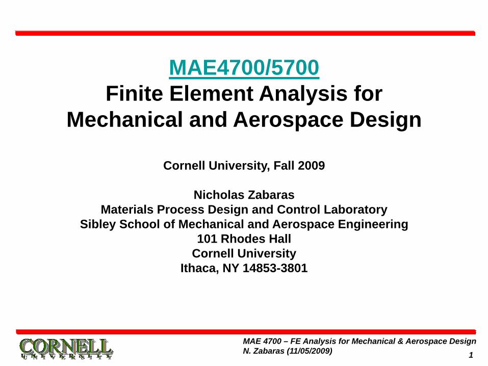
• Extension to 3D is very easy. For example, the equilibrium equations take the form:
• The traction/stress relation is now:
Elastic deformations in 3D
0 0 0
0, : 0 0 0
0 0 0
xx
yy
zzT TS S
xy
xz
yz
x y z
b where andy x z
z x y
⎡ ⎤∂ ∂ ∂⎡ ⎤ ⎢ ⎥⎢ ⎥∂ ∂ ∂ ⎢ ⎥⎢ ⎥ ⎢ ⎥∂ ∂ ∂⎢ ⎥ ⎢ ⎥∇ + = ∇ = =⎢ ⎥∂ ∂ ∂ ⎢ ⎥⎢ ⎥ ⎢ ⎥∂ ∂ ∂⎢ ⎥ ⎢ ⎥⎢ ⎥∂ ∂ ∂⎣ ⎦ ⎢ ⎥⎣ ⎦
σσ
σσ σ
σ
σσ
xx xy xzx x
y xy yy yz y
z xz yz zz z
t nt t n
t n
⎡ ⎤⎡ ⎤ ⎡ ⎤⎢ ⎥⎢ ⎥ ⎢ ⎥= = ⎢ ⎥⎢ ⎥ ⎢ ⎥⎢ ⎥⎢ ⎥ ⎢ ⎥⎣ ⎦ ⎣ ⎦⎣ ⎦
σ σ σ
σ σ σ
σ σ σ

4MAE 4700 – FE Analysis for Mechanical & Aerospace DesignN. Zabaras (11/05/2009)
• The strain/displacement relation is simply:
• The isotropic Hooke’s law takes the form:
Elastic deformations in 3D0 0
0 0
0 0,
0
0
0
xx
yyx
zzy S
xyz
xz
yz
x
y
uz u u where
uy x
z x
z y
∂⎡ ⎤⎢ ⎥∂⎢ ⎥∂⎢ ⎥ ⎡ ⎤⎢ ⎥∂ ⎢ ⎥⎢ ⎥∂ ⎢ ⎥⎢ ⎥ ⎡ ⎤ ⎢ ⎥∂⎢ ⎥ ⎢ ⎥ ⎢ ⎥= = ∇ =⎢ ⎥ ⎢ ⎥∂ ∂ ⎢ ⎥⎢ ⎥ ⎢ ⎥⎣ ⎦ ⎢ ⎥∂ ∂⎢ ⎥ ⎢ ⎥⎢ ⎥∂ ∂ ⎢ ⎥⎣ ⎦⎢ ⎥∂ ∂⎢ ⎥
∂ ∂⎢ ⎥⎢ ⎥∂ ∂⎣ ⎦
εε
εε ε
γ
γγ
1 0 0 01 0 0 0
1 0 0 01 20 0 0 0 0
2(1 )(1 2 )1 20 0 0 0 0
21 20 0 0 0 0
2
ED
−⎡ ⎤⎢ ⎥−⎢ ⎥
−⎢ ⎥⎢ ⎥−⎢ ⎥= ⎢ ⎥+ −⎢ ⎥−⎢ ⎥⎢ ⎥
−⎢ ⎥⎢ ⎥⎣ ⎦
υ υ υυ υ υυ υ υ
υ
υ υυ
υ
D=σ ε

5MAE 4700 – FE Analysis for Mechanical & Aerospace DesignN. Zabaras (11/05/2009)
Standard 3D solid element geometries
Tetrahedron (tet) Pentahedron (wedge) Hexahedron (brick)
These are element geometries with corner nodes only
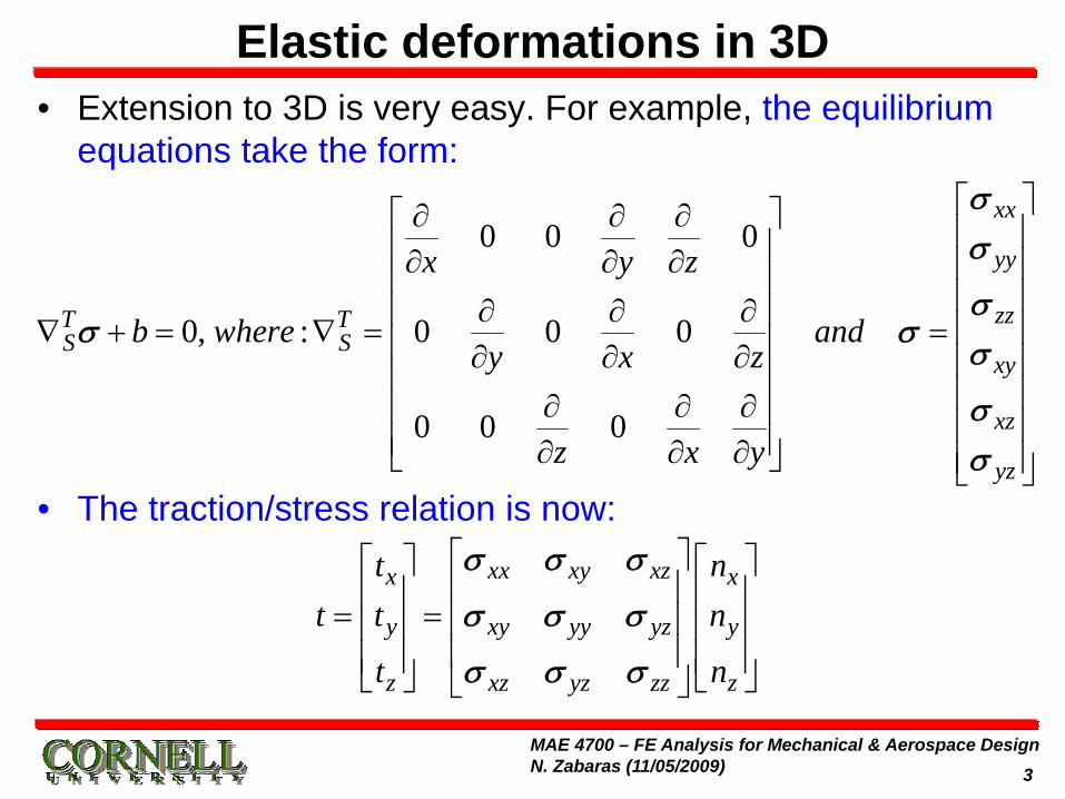
6MAE 4700 – FE Analysis for Mechanical & Aerospace DesignN. Zabaras (11/05/2009)
Solid elements with midpoints

7MAE 4700 – FE Analysis for Mechanical & Aerospace DesignN. Zabaras (11/05/2009)
3D Finite Elements: Hexahedral elements• This is an 8-node element. The shape functions are
constructed by tensor product of 1D linear shape functions.
( ) ( )1 2
( ) ( )3 4
( ) ( )5 6
( ) ( )7 8
1 1(1 )(1 )(1 ), (1 )(1 )(1 )8 81 1(1 )(1 )(1 ), (1 )(1 )(1 )8 81 1(1 )(1 )(1 ), (1 )(1 )(1 )8 81 1(1 )(1 )(1 ), (1 )(1 )(1 )8 8
e e
e e
e e
e e
N N
N N
N N
N N
= − − − = + − −
= + + − = − + −
= − − + = + − +
= + + + = − + +
ξ η ζ ξ η ζ
ξ η ζ ξ η ζ
ξ η ζ ξ η ζ
ξ η ζ ξ η ζ
( )
:1 (1 )(1 )(1 ), 1,...,88
( , , ) :
ei i ii
i i i
or in compact format
N i
master coordinates of node i
= + + + =ξξ ηη ζζ
ξ η ζ
ζ
8MAE 4700 – FE Analysis for Mechanical & Aerospace DesignN. Zabaras (11/05/2009)
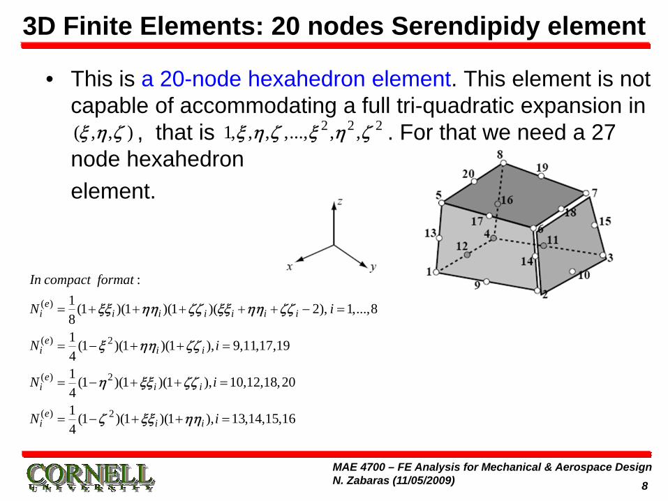
• This is a 20-node hexahedron element. This element is not capable of accommodating a full tri-quadratic expansion in
, that is . For that we need a 27 node hexahedron element.
3D Finite Elements: 20 nodes Serendipidy element
2 2 21, , , ,..., , ,ξ η ζ ξ η ζ( , , )ξ η ζ
( )
( ) 2
( ) 2
( ) 2
:1 (1 )(1 )(1 )( 2), 1,...,881 (1 )(1 )(1 ), 9,11,17,1941 (1 )(1 )(1 ), 10,12,18,2041 (1 )(1 )(1 ), 13,14,15,164
ei i i i i ii
ei ii
ei ii
ei ii
In compact format
N i
N i
N i
N i
= + + + + + − =
= − + + =
= − + + =
= − + + =
ξξ ηη ζζ ξξ ηη ζζ
ξ ηη ζζ
η ξξ ζζ
ζ ξξ ηη

9MAE 4700 – FE Analysis for Mechanical & Aerospace DesignN. Zabaras (11/05/2009)
3D Finite Elements: 27 node Hexahedron
• A 27-node hexahedron can be constructed by adding 7 more nodes:6 one each face center and 1 interior node at the hexahedron center.
• In elasticity application such an element has 27×3=81 degrees of freedom!
10MAE 4700 – FE Analysis for Mechanical & Aerospace DesignN. Zabaras (11/05/2009)
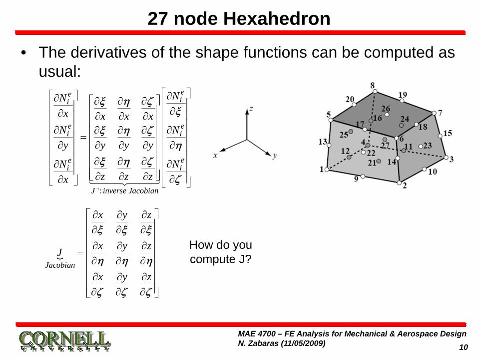
27 node Hexahedron
• The derivatives of the shape functions can be computed as usual:
1:
eeii
e ei i
eeii
J inverse Jacobian
NNx x x x
N Ny y y y
NNz z zx
−
⎡ ⎤∂⎡ ⎤∂ ∂ ∂ ∂⎡ ⎤ ⎢ ⎥⎢ ⎥ ∂⎢ ⎥∂ ⎢ ⎥∂ ∂ ∂⎢ ⎥ ⎢ ⎥ ⎢ ⎥⎢ ⎥∂ ∂∂ ∂ ∂⎢ ⎥ ⎢ ⎥=⎢ ⎥ ⎢ ⎥∂ ∂ ∂ ∂ ∂⎢ ⎥⎢ ⎥ ⎢ ⎥ ⎢ ⎥⎢ ⎥ ∂ ∂ ∂ ∂∂ ⎢ ⎥ ⎢ ⎥⎢ ⎥ ⎢ ⎥⎣ ⎦∂ ∂ ∂ ⎢ ⎥∂∂⎣ ⎦ ⎣ ⎦
ξ η ζξ
ξ η ζη
ξ η ζ
ζ
Jacobian
x y z
x y zJ
x y z
∂ ∂ ∂⎡ ⎤⎢ ⎥∂ ∂ ∂⎢ ⎥∂ ∂ ∂⎢ ⎥= ⎢ ⎥∂ ∂ ∂
⎢ ⎥∂ ∂ ∂⎢ ⎥
⎢ ⎥∂ ∂ ∂⎣ ⎦
ξ ξ ξ
η η η
ζ ζ ζ
How do youcompute J?

11MAE 4700 – FE Analysis for Mechanical & Aerospace DesignN. Zabaras (11/05/2009)
27 node Hexahedron
• The Jacobian can be computed using the isoparametric map:
Gauss integration using a tensor product of 1D integration rules will finally give:
e e ei i i i i i
i i i
e e ei i i i i i
i i i
Jacobiane e e
i i i i i ii i i
e e ei i i
i i ii i i
e e ei i i
i i ii i i
ei
i ii
x N y N z N
x N y N z NJ
x N y N z N
N N Nx y z
N N Nx y z
N Nx y
∑ ∑ ∑
∑ ∑ ∑
∑ ∑ ∑
∑ ∑ ∑
∑ ∑ ∑
∑
⎡ ⎤∂ ∂ ∂⎢ ⎥⎢ ⎥∂ ∂ ∂⎢ ⎥∂ ∂ ∂⎢ ⎥⎢ ⎥= =⎢ ⎥∂ ∂ ∂⎢ ⎥∂ ∂ ∂⎢ ⎥⎢ ⎥
∂ ∂ ∂⎢ ⎥⎣ ⎦
∂ ∂ ∂∂ ∂ ∂
∂ ∂ ∂=
∂ ∂ ∂
∂ ∂∂
ξ ξ ξ
η η η
ζ ζ ζ
ξ ξ ξ
η η η
ζ
e ei i
ii i
Nz∑ ∑
⎡ ⎤⎢ ⎥⎢ ⎥⎢ ⎥⎢ ⎥⎢ ⎥⎢ ⎥∂⎢ ⎥⎢ ⎥∂ ∂⎣ ⎦ζ ζ
( )( , , )1 1 1| |
TGauss Gauss Gauss
i j k
N N Ne e e ei j k
i j kK WW W B D B J
= = =∑ ∑ ∑=
ξ η ζ

12MAE 4700 – FE Analysis for Mechanical & Aerospace DesignN. Zabaras (11/05/2009)
• This is not used in deformation problems (poor performance).
• We use natural coordinates as for the 3 node triangular element.
• The volume of the tetrahedron is given as:
• For V>0, the nodes need to be numbered properly:– For any face, the corners are numbered in a counterclockwise sense when
looking at the face from the excluded corner.
The linear tetrahedron
1 2 3 4
1 2 3 4
1 2 3 4
1 1 1 11 det6
x x x xV
y y y yz z z z
⎡ ⎤⎢ ⎥⎢ ⎥=⎢ ⎥⎢ ⎥⎣ ⎦
Phase 123 seen fromnode 4

13MAE 4700 – FE Analysis for Mechanical & Aerospace DesignN. Zabaras (11/05/2009)
• The four coordinates are relatedas
• Each is 1 at node iand zero at the remaining nodes andvaries linearly as we transverse the distance from the corner i to the face.
• These coordinates can be easily computed in terms of x,y,z as follows:
Linear tetrahedron:tetrahedral coordinates
1 2 3 4 1+ + + =ζ ζ ζ ζ
1
1 2 3 4 2
1 2 3 4 3
1 2 3 4 4
1 1 1 11x x x xxy y y yyz z z zz
⎡ ⎤ ⎡ ⎤⎡ ⎤⎢ ⎥ ⎢ ⎥⎢ ⎥⎢ ⎥ ⎢ ⎥⎢ ⎥ = ⇒⎢ ⎥ ⎢ ⎥⎢ ⎥⎢ ⎥ ⎢ ⎥⎢ ⎥
⎣ ⎦ ⎣ ⎦⎣ ⎦
ζζζζ
1 1 1 1 1
2 2 2 2 2
3 3 3 3 3
4 4 4 4 4
6 161666
V a b cV a b c xV a b c yVV a b c z
⎡ ⎤ ⎡ ⎤ ⎡ ⎤⎢ ⎥ ⎢ ⎥ ⎢ ⎥⎢ ⎥ ⎢ ⎥ ⎢ ⎥=⎢ ⎥ ⎢ ⎥ ⎢ ⎥⎢ ⎥ ⎢ ⎥ ⎢ ⎥
⎣ ⎦⎣ ⎦ ⎣ ⎦
ζζζζ
iζ
1 2 43 3 42 4 32
1 2 43 3 42 4 32
1 2 43 3 42 4 32, .: ,ij i j ij i j
a y z y z y zb x z x z x zc x y x y x y etcwhere z z z y y y
= − +
= − + −
= − +
= − = −

14MAE 4700 – FE Analysis for Mechanical & Aerospace DesignN. Zabaras (11/05/2009)
• From the above expression, note that:
• Thus differentiation with respect to x,y,z can proceed as:
Linear tetrahedron:computing derivatives
, ,6 6 6
i i i i i ia b cx V y V z V
∂ ∂ ∂= = =
∂ ∂ ∂ζ ζ ζ
1 1 1 1 1
2 2 2 2 2
3 3 3 3 3
4 4 4 4 4
6 161666
V a b cV a b c xV a b c yVV a b c z
⎡ ⎤ ⎡ ⎤ ⎡ ⎤⎢ ⎥ ⎢ ⎥ ⎢ ⎥⎢ ⎥ ⎢ ⎥ ⎢ ⎥=⎢ ⎥ ⎢ ⎥ ⎢ ⎥⎢ ⎥ ⎢ ⎥ ⎢ ⎥
⎣ ⎦⎣ ⎦ ⎣ ⎦
ζζζζ
31 2 4
1 2 3 4
31 2 4
1 2 3 4, .
6 6 6 6
x x x x xaa a a etc
V V V V
∂∂ ∂ ∂∂ ∂ ∂ ∂ ∂= + + + =
∂ ∂ ∂ ∂ ∂ ∂ ∂ ∂ ∂
∂ ∂ ∂ ∂= + + +∂ ∂ ∂ ∂
ζζ ζ ζζ ζ ζ ζ
ζ ζ ζ ζ

15MAE 4700 – FE Analysis for Mechanical & Aerospace DesignN. Zabaras (11/05/2009)
• Recall that the strains are computed as:
• The displacements are approximated as:
Linear tetrahedron: Constant strain0 0
0 0
0 0,
0
0
0
xx
yyx
zzy S
xyz
xz
yz
x
y
uz u u where
uy x
z x
z y
∂⎡ ⎤⎢ ⎥∂⎢ ⎥
∂⎢ ⎥ ⎡ ⎤⎢ ⎥∂ ⎢ ⎥⎢ ⎥∂ ⎢ ⎥⎢ ⎥ ⎡ ⎤ ⎢ ⎥∂⎢ ⎥ ⎢ ⎥ ⎢ ⎥= = ∇ =⎢ ⎥ ⎢ ⎥∂ ∂ ⎢ ⎥⎢ ⎥ ⎢ ⎥⎣ ⎦ ⎢ ⎥∂ ∂⎢ ⎥ ⎢ ⎥⎢ ⎥∂ ∂ ⎢ ⎥⎣ ⎦⎢ ⎥∂ ∂⎢ ⎥
∂ ∂⎢ ⎥⎢ ⎥∂ ∂⎣ ⎦
εε
εε ε
γ
γγ
1
1
1
2
1 2 3 4
1 2 3 4
1 2 3 4
4
4
4
...0 0 0 0 0 0 0 0
..0 0 0 0 0 0 0 00 0 0 0 0 0 0 0
x
y
z
x
x
y
z
x
y
z
uu
uu
uu
u
uu
u
⎡ ⎤⎢ ⎥⎢ ⎥⎢ ⎥⎢ ⎥⎢ ⎥⎢ ⎥
⎡ ⎤ ⎢ ⎥⎡ ⎤⎢ ⎥ ⎢ ⎥⎢ ⎥=⎢ ⎥ ⎢ ⎥⎢ ⎥⎢ ⎥ ⎢ ⎥⎢ ⎥⎣ ⎦⎣ ⎦ ⎢ ⎥
⎢ ⎥⎢ ⎥⎢ ⎥⎢ ⎥⎢ ⎥⎢ ⎥⎣ ⎦
ζ ζ ζ ζζ ζ ζ ζ
ζ ζ ζ ζ

16MAE 4700 – FE Analysis for Mechanical & Aerospace DesignN. Zabaras (11/05/2009)
• Thus the B matrix is:
Linear tetrahedron: Constant strain
1 2 3 4
1 2 3 4
1 2 3 4
1 2 3 4
1 2 3 4
1 2 3 4
1 1 2 2 3 3 4
0 0
0 0
0 0 0 0 0 0 0 00 00 0 0 0 0 0 0 0
0 0 0 0 0 0 0 0 0
0
0
0 0 0 0 0 0 0 00 0 0 0 0 0 0 00 0 0 0 0 0 0 01
0 0 06
x
y
zB
y x
z x
z ya a a a
b b b bc c c c
b a b a b a bV
∂⎡ ⎤⎢ ⎥∂⎢ ⎥
∂⎢ ⎥⎢ ⎥∂⎢ ⎥∂⎢ ⎥ ⎡ ⎤
∂⎢ ⎥ ⎢ ⎥= =⎢ ⎥ ⎢ ⎥∂ ∂⎢ ⎥ ⎢ ⎥⎣ ⎦∂ ∂⎢ ⎥⎢ ⎥∂ ∂⎢ ⎥∂ ∂⎢ ⎥
∂ ∂⎢ ⎥⎢ ⎥∂ ∂⎣ ⎦
=
ζ ζ ζ ζζ ζ ζ ζ
ζ ζ ζ ζ
4
1 1 2 2 3 3 4 4
1 1 2 2 3 3 4 4
.0
0 0 0 00 0 0 0
consta
c a c a c a c ac b c b c b c b
⎡ ⎤⎢ ⎥⎢ ⎥⎢ ⎥
=⎢ ⎥⎢ ⎥⎢ ⎥⎢ ⎥⎣ ⎦

17MAE 4700 – FE Analysis for Mechanical & Aerospace DesignN. Zabaras (11/05/2009)
• For calculating volume integrals, the following rule is very useful:
• For example, for constant body forces, you will need integrals of the form:
Linear tetrahedron: Constant strain
1 3 42! ! ! ! 6 , , , , int
( 3)!e
ji k l i j k ld V i j k l non negative egersi j k lΩ
∫ Ω = = −+ + + +
ζ ζ ζ ζ
1! 16 6(4)! 1234 4e
mVd V V
Ω∫ Ω = = =ζ

18MAE 4700 – FE Analysis for Mechanical & Aerospace DesignN. Zabaras (11/05/2009)
Quadratic tetrahedron
• The shape functions are written in terms of natural coordinates as:
( ) ( )1 1 2 21 2
( ) ( )3 3 4 43 4
( ) ( )1 2 2 35 6
( ) ( )3 1 1 47 8
( ) ( )2 4 3 49 10
:
(2 1), (2 1)
(2 1), (2 1)
4 , 4
4 , 4
4 , 4
e e
e e
e e
e e
e e
In compact format
N N
N N
N N
N N
N N
= − = −
= − = −
= =
= =
= =
ζ ζ ζ ζ
ζ ζ ζ ζ
ζ ζ ζ ζ
ζ ζ ζ ζ
ζ ζ ζ ζ

19MAE 4700 – FE Analysis for Mechanical & Aerospace DesignN. Zabaras (11/05/2009)
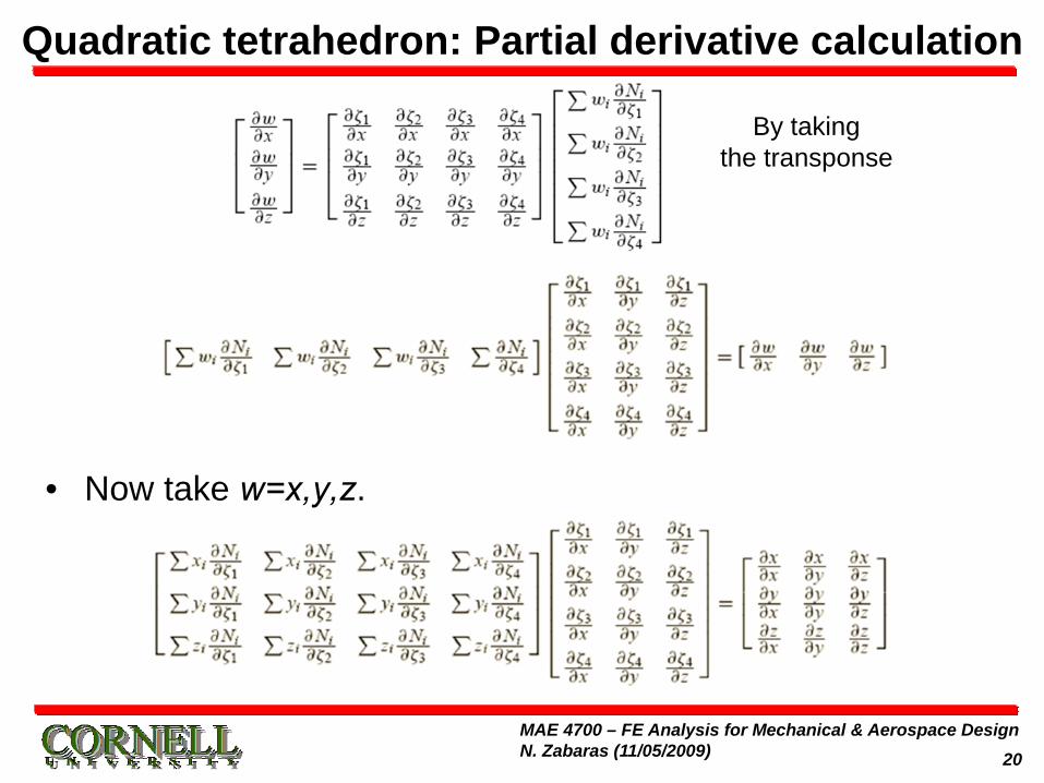
Quadratic tetrahedron: Partial derivative calculation
• Consider the interpolation of any arbitrary function w.
• The partial derivatives are computed as:
20MAE 4700 – FE Analysis for Mechanical & Aerospace DesignN. Zabaras (11/05/2009)
Quadratic tetrahedron: Partial derivative calculation
• Now take w=x,y,z.
By takingthe transponse
21MAE 4700 – FE Analysis for Mechanical & Aerospace DesignN. Zabaras (11/05/2009)
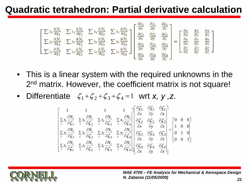
Quadratic tetrahedron: Partial derivative calculation
• This is a linear system with the required unknowns in the 2nd matrix. However, the coefficient matrix is not square!
• Differentiate wrt x, y ,z.1 2 3 4 1+ + + =ζ ζ ζ ζ
1 1 1
2 2 21 2 3 4
3 3 31 2 3 4
4 41 2 3 4
1 1 1 1
i i i ii i i i
i i i i
i i i ii i i i
i i i i
i i i ii i i i
i i i i
x y zN N N Nx x x x
x y zN N N Ny y y y
x y zN N N Nz z z z
x
∑ ∑ ∑ ∑
∑ ∑ ∑ ∑
∑ ∑ ∑ ∑
∂ ∂ ∂⎡ ⎤
∂ ∂ ∂⎢ ⎥∂ ∂ ∂ ∂⎢ ⎥ ∂ ∂ ∂∂ ∂ ∂ ∂⎢ ⎥
∂ ∂ ∂⎢ ⎥∂ ∂ ∂ ∂⎢ ⎥ ∂ ∂ ∂∂ ∂ ∂ ∂⎢ ⎥ ∂ ∂ ∂⎢ ⎥∂ ∂ ∂ ∂⎢ ⎥ ∂ ∂∂ ∂ ∂ ∂⎢ ⎥⎣ ⎦ ∂ ∂
ζ ζ ζ
ζ ζ ζζ ζ ζ ζ
ζ ζ ζζ ζ ζ ζ
ζ ζζ ζ ζ ζ 4
0 0 01 0 00 1 00 0 1
y z
⎡ ⎤⎢ ⎥⎢ ⎥
⎡ ⎤⎢ ⎥⎢ ⎥⎢ ⎥⎢ ⎥⎢ ⎥ =⎢ ⎥⎢ ⎥⎢ ⎥⎢ ⎥ ⎣ ⎦⎢ ⎥
∂⎢ ⎥⎢ ⎥∂⎣ ⎦
ζ

22MAE 4700 – FE Analysis for Mechanical & Aerospace DesignN. Zabaras (11/05/2009)
Quadratic tetrahedron: Partial derivative calculation
• Once you solve these system of linear equations for the derivatives on the 2nd matrix, you can then compute the partial derivatives of w from an earlier equation as follows:
1 1 1
2 2 21 2 3 4
3 3 31 2 3 4
4 41 2 3 4
1 1 1 1
i i i ii i i i
i i i i
i i i ii i i i
i i i i
i i i ii i i i
i i i i
x y zN N N Nx x x x
x y zN N N Ny y y y
x y zN N N Nz z z z
x
∑ ∑ ∑ ∑
∑ ∑ ∑ ∑
∑ ∑ ∑ ∑
∂ ∂ ∂⎡ ⎤
∂ ∂ ∂⎢ ⎥∂ ∂ ∂ ∂⎢ ⎥ ∂ ∂ ∂∂ ∂ ∂ ∂⎢ ⎥
∂ ∂ ∂⎢ ⎥∂ ∂ ∂ ∂⎢ ⎥ ∂ ∂ ∂∂ ∂ ∂ ∂⎢ ⎥ ∂ ∂ ∂⎢ ⎥∂ ∂ ∂ ∂⎢ ⎥ ∂ ∂∂ ∂ ∂ ∂⎢ ⎥⎣ ⎦ ∂ ∂
ζ ζ ζ
ζ ζ ζζ ζ ζ ζ
ζ ζ ζζ ζ ζ ζ
ζ ζζ ζ ζ ζ 4
0 0 01 0 00 1 00 0 1
y z
⎡ ⎤⎢ ⎥⎢ ⎥
⎡ ⎤⎢ ⎥⎢ ⎥⎢ ⎥⎢ ⎥⎢ ⎥ =⎢ ⎥⎢ ⎥⎢ ⎥⎢ ⎥ ⎣ ⎦⎢ ⎥
∂⎢ ⎥⎢ ⎥∂⎣ ⎦
ζ

23MAE 4700 – FE Analysis for Mechanical & Aerospace DesignN. Zabaras (11/05/2009)
Quadratic tetrahedron: Partial derivative calculation
• For transforming integration from to
you can show that
1 2 3 4ed Jd d d dΩ = ζ ζ ζ ζ
edΩ 1 2 3 4d d d dζ ζ ζ ζ
1 2 3 4
1 2 3 4
1 2 3 4
1 1 1 1
1 det6
i i i ii i i i
i i i i
i i i ii i i i
i i i i
i i i ii i i i
i i i i
N N N Nx x x x
J N N N Ny y y y
N N N Nz z z z
∑ ∑ ∑ ∑
∑ ∑ ∑ ∑
∑ ∑ ∑ ∑
⎡ ⎤⎢ ⎥∂ ∂ ∂ ∂⎢ ⎥
∂ ∂ ∂ ∂⎢ ⎥⎢ ⎥= ∂ ∂ ∂ ∂⎢ ⎥
∂ ∂ ∂ ∂⎢ ⎥⎢ ⎥∂ ∂ ∂ ∂⎢ ⎥
∂ ∂ ∂ ∂⎢ ⎥⎣ ⎦
ζ ζ ζ ζ
ζ ζ ζ ζ
ζ ζ ζ ζ
24MAE 4700 – FE Analysis for Mechanical & Aerospace DesignN. Zabaras (11/05/2009)
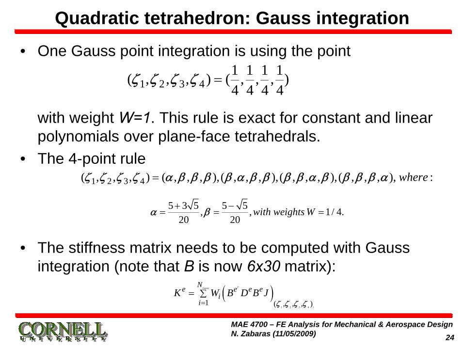
Quadratic tetrahedron: Gauss integration
• One Gauss point integration is using the point
with weight W=1. This rule is exact for constant and linear polynomials over plane-face tetrahedrals.
• The 4-point rule
• The stiffness matrix needs to be computed with Gauss integration (note that B is now 6x30 matrix):
5 3 5 5 5, , 1/ 4.20 20
with weights W+ −= = =α β
1 2 3 41 1 1 1( , , , ) ( , , , )4 4 4 4
=ζ ζ ζ ζ
1 2 3 4( , , , ) ( , , , ), ( , , , ), ( , , , ), ( , , , ), :where=ζ ζ ζ ζ α β β β β α β β β β α β β β β α
( )1 2 3 4
1 ( , , , )
TGauss
i
Ne e e ei
iK W B D B J
=∑=
ζ ζ ζ ζ
25MAE 4700 – FE Analysis for Mechanical & Aerospace DesignN. Zabaras (11/05/2009)
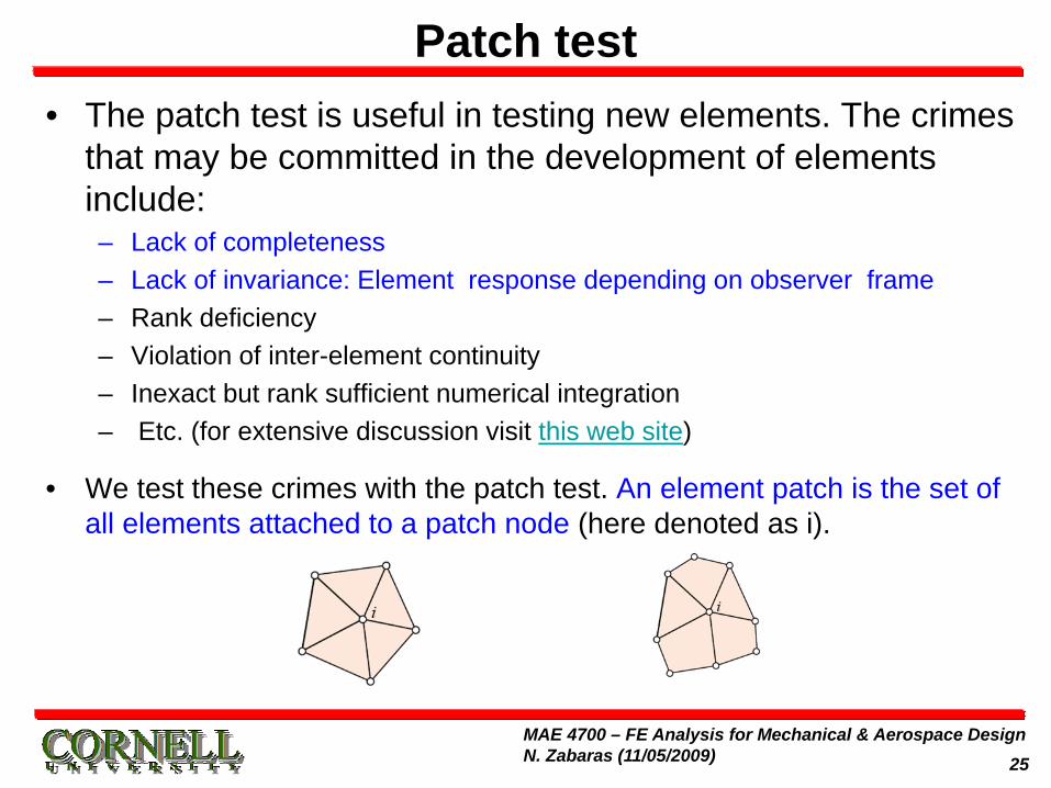
• The patch test is useful in testing new elements. The crimes that may be committed in the development of elements include:– Lack of completeness– Lack of invariance: Element response depending on observer frame– Rank deficiency– Violation of inter-element continuity– Inexact but rank sufficient numerical integration– Etc. (for extensive discussion visit this web site)
• We test these crimes with the patch test. An element patch is the set of all elements attached to a patch node (here denoted as i).
Patch test
26MAE 4700 – FE Analysis for Mechanical & Aerospace DesignN. Zabaras (11/05/2009)
• A good finite element must solve simple problems exactly whether individually, or as component of arbitrary patches.
• To create simple problems, think of a mesh refinement process. For example, at the limit of refinement, the stress/strain states are uniform within each element.
• The patch test has two dual forms:
– Displacement Patch Test : applies boundary displacements to patch and verifies that the patch response reproduces exactly rigid body modes and constant strain states.
– Force Patch Test: applies boundary forces to patch and verifies that the patch response reproduces exactly constant stress states.
– There are also mixed patch tests that incorporate both force and displacement BCs.
Patch test

27MAE 4700 – FE Analysis for Mechanical & Aerospace DesignN. Zabaras (11/05/2009)
• Pick a patch. At the external nodes of the patch apply rigid body motion as prescribed displacements. Set forces at interior DOFs to zero.
• Solve for the displacement components of the interior nodes. These should agree with the value of the displacement field at that node.
• Recover the strain field over the elements: all components should vanish identically at any point.
Displacement Patch Test: translation in x-direction

28MAE 4700 – FE Analysis for Mechanical & Aerospace DesignN. Zabaras (11/05/2009)
• We apply a constant-strain-mode ux = x and uy = 0 at the external nodes of the patch. This gives exx = ∂ux/∂x = 1, others zero. We set the forces at the internal nodes to zero.
• We solve for the displacements of interior nodes. They should agree with the value of the displacement field at that node.
• We need to also recover the strain field over the elements: all components should vanish except exx = 1 at any point.
• If the displacement/strain states are reproduced correctly, the patch test is passed.
Displacement Patch Test: constant exx

29MAE 4700 – FE Analysis for Mechanical & Aerospace DesignN. Zabaras (11/05/2009)
• We consider a patch test with uniform stress σxx = 1, others zero. On the boundary of the patch we apply a uniform traction tx = σxx. Convert this to nodal forces using a consistent force lumping approach. Forces at interior DOFs should be zero.
• We need to apply a minimal number of displacement BC to eliminate rigid body motions.
• Solve for displacements, strains & stresses over the elements. The computed stresses should recover exactly the test state.
• If all test states are reproduced, the test is passed.
A force patch test: σxx=1

30MAE 4700 – FE Analysis for Mechanical & Aerospace DesignN. Zabaras (11/05/2009)
• You already have noticed from the computer assignments that the stresses are always computed at the Gauss points.
• Calculation of the derivatives of the basis functions (thus of strains and stresses) at the Gauss points is optimal (see Hughes for more details).
• How do we compute nodal stresses from the values of the stresses at the Gauss points? – We use a global least squares approach.
• Let us work with a particular stress component σ. We would like to compute the nodal strsses σi from the Gauss stress σG (known only at the Gauss points of each element).
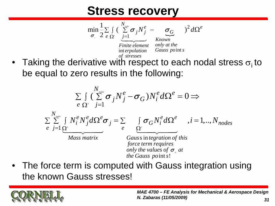
Stress recovery
2
1
intint
1min ( )2
nodes
ei
N e ej j G
e j Knownonly at theFinite elementGauss po serpolation
of stresses
N d=Ω
∑ ∑∫ − Ωσ
σ σ
31MAE 4700 – FE Analysis for Mechanical & Aerospace DesignN. Zabaras (11/05/2009)
• Taking the derivative with respect to each nodal stress σi to be equal to zero results in the following:
• The force term is computed with Gauss integration using the known Gauss stresses!
Stress recovery2
1
intint
1min ( )2
nodes
ei
N e ej j G
e j Knownonly at theFinite elementGauss po serpolation
of stresses
N d=Ω
∑ ∑∫ − Ωσ
σ σ
1( ) 0
nodes
e
N e e ej j G i
e jN N d
=Ω∑ ∑∫ − Ω = ⇒σ σ
1
s in
int !
, 1,..,nodes
e e
G
N e e e e ei j j G i nodes
e j e
Mass matrix Gaus tegration of thisforce term requiresonly the values of atthe Gauss po s
N N d N d i N= Ω Ω
∑ ∑ ∑∫ ∫Ω = Ω =
σ
σ σ