1

Module 10a: Storm

Sewer

Design

Bob Pitt

University of Alabama

and

Shirley Clark

Penn State –Harrisburg

A trailer is trapped under a bridge

by floodwaters, Houston, TX.

Photo by Mary Grove.

Major floods are dramatic

and water flow routes m

ust

be recognized when m

inor

drainage systems fail.

These types of events are

not directly addressed by

typical storm

drainage

systems (the m

inor

systems).

A sheriff's car is not able to escape rising floodwaters.

Photo by Cindy Cruz.

Siren lights on this submerged firetruckare still flashing on the East Loop at I-10.

Photo by Paul Carrizales.

2

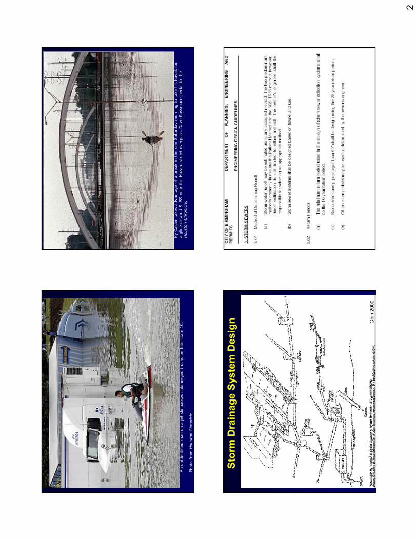
An unidentified man on a jet ski passes submerged trucks on Interstate 10.

Photo from Houston Chronicle.

KyCalder takes advantage of a break in the rain Saturday morning to take his kayak for

a glide down U.S. 59 near the Hazard street overpass. Dave Rossmanspecial to the

Houston Chronicle.

Storm

Drainage System Design Chin 2000

3

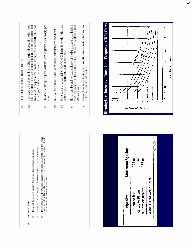
Chin 2000

Bir

min

gham

Inte

nsi

ty -

Dura

tion -

Fre

quen

cy (

IDF

) C

urv

e

4

Pipe AB: inlet tc= 6 min; i = 7.4 in/hr; Q = CiA

= (0.3)(7.4 in/hr)(3.1 acres) = 6.9 cfs

Determ

ine “10-yr”

(10% probability of being exceeded in any one year)

flows at inlets to pipes:

Pipe BC: inlet tc= 8 min vs. 6 +0.6 m

in, use 8 min; i = 6.6 in/hr;

Q= [(3.1ac)(0.3)+(2.8ac)(0.4)] 6.6 in/hr = 13.5 cfs

Pipe CD: inlet tc= 5 min vs. 6 + 0.6 + 0.5 vs. 8 + 0.5, use 8.5 min; i = 6.3 in/hr;

Q = [(3.1ac)(0.3)+(2.8ac)(0.4)+(2.1ac)(0.35)] 6.3 in/hr = 17.5 cfs

The travel times in the pipes can only be calculated after the pipe sizes are selected

and the velocities at the design flows are determ

ined.

Basic Application of Rational Form

ula:

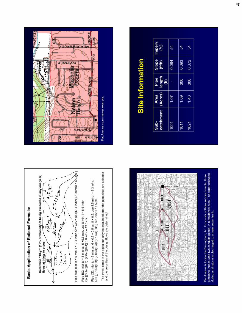
Pat Avenue storm

sewer example.

Pat Avenue is located in Birmingham, AL. It consists of three subcatchments, three

junctions (nodes) and two conduits (pipes) in a residential area. The water collected

during a rainstorm

is discharged to a m

ain sewer trunk.

1000

1001

Site Inform

ation

54

0.072

300

1.43

1021

54

0.093

300

1.09

1011

54

0.084

-1.07

1001

Imperv.

(%)

Slope

(ft/ft)

Pipe

length

(ft)

Area

(Acres)

Sub-

catchment

5

Runoff Coefficients for the Rational Form

ula for Different

Hydrologic Soil Groups (A, B, C, D) and Slope Ranges

(from McCuen, Hydrologic Analysis and Design. Prentice-Hall, Inc. 1998)

0.46

0.35

0.31

0.40

0.32

0.28

0.34

0.28

0.2

0.29

0.26

0.22

0.35

0.29

0.24

0.31

0.25

0.20

0.26

0.21

0.17

0.22

0.19

0.14

Residential

Lot, 1 acre

0.90

0.89

0.89

0.90

0.89

0.89

0.89

0.89

0.89

0.89

0.88

0.88

0.72

0.72

0.72

0.72

0.72

0.72

0.72

0.72

0.71

0.72

0.71

0.71

Commer-

cial

0.48

0.38

0.34

0.42

0.35

0.31

0.36

0.32

0.28

0.32

0.29

0.25

0.37

0.30

0.26

0.32

0.27

0.22

0.28

0.23

0.19

0.24

0.20

0.16

Residential

Lot, ½

acre

0.50

0.40

0.36

0.45

0.38

0.33

0.39

0.35

0.30

0.35

0.32

0.28

0.39

0.32

0.28

0.34

0.29

0.25

0.30

0.26

0.22

0.26

0.23

0.19

Residential

Lot, ⅓

acre

0.52

0.42

0.38

0.47

0.40

0.36

0.42

0.37

0.33

0.37

0.34

0.30

0.40

0.34

0.30

0.36

0.31

0.27

0.33

0.29

0.24

0.29

0.26

0.22

Residential

Lot, ¼

acre

0.54

0.45

0.41

0.49

0.42

0.38

0.44

0.39

0.35

0.40

0.37

0.33b

0.42

0.36

0.33

0.38

0.33

0.30

0.35

0.30

0.27

0.31

0.28

0.25a

Residential

Lot, ⅛

acre

6% +

2–6%

0–

2%

6%+

2–6%

0–

2%

6%+

2–6%

0–

2%

6%+

2–6%

0–

2%

DC

BA

Land Use

aRunoff coefficients for storm

recurrence intervals less than 25years.

bRunoff coefficients for storm

recurrence intervals of 25 years or longer.

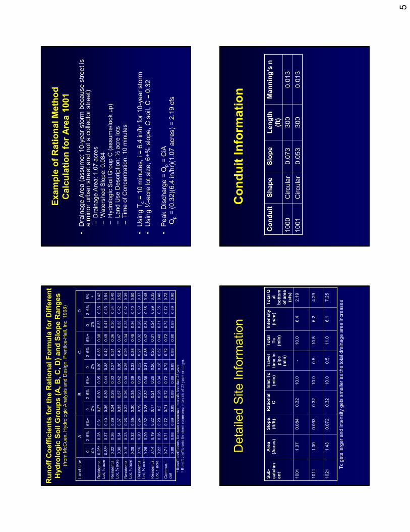
Example of Rational Method

Calculation for Area 1001

•Drainage Area (assume: 10-year storm

because street is

a m

inor urban street and not a collector street)

–Drainage Area: 1.07 acres

–Watershed Slope: 0.084

–Hydrologic Soil Group C (assume/look up)

–Land Use Description: ½acre lots

–Time of Concentration: 10 m

inutes

•Using T

c= 10 m

inutes, i = 6.4 in/hr for 10-year storm

•Using ½-acre lot size, 6+% slope, C soil, C = 0.32

•Peak Discharge = Q

p= CiA

Qp= (0.32)(6.4 in/hr)(1.07 acres) = 2.19 cfs

Detailed Site Inform

ation

11.0

10.5

10.0

Total

Tc

(min)

0.5

0.5-

Travel

time in

pipe

(min)

0.32

0.32

0.32

Rational

C

7.25

6.1

10.0

0.072

1.43

1021

4.29

6.2

10.0

0.093

1.09

1011

2.19

6.4

10.0

0.084

1.07

1001

Total Q

at

bottom

of area

(cfs)

Intensity

(in/hr)

Inlet Tc

(min)

Slope

(ft/ft)

Area

(Acres)

Sub-

catchm

ent

Tcgets larger and intensity gets smaller as the total drainage area increases

Conduit Inform

ation

0.013

300

0.053

Circular

1001

0.013

300

0.073

Circular

1000

Manning’s n

Length

(ft)

Slope

Shape

Conduit

6

Manning’s Equation

Diameter of a

Pipe Flowing

Full Using

Manning’s

Equation for

Flow

DSnQ

DSnQ

D

S

nQ

DD

S

nQ

DD

S

nQ

SD

Dn

Q

=

==

=

=

=

8/3

2/

1

3/

5

3/

8

2/

1

3/5

3/

2

3/

8

2/

1

3/

2

2

2/

1

3/

2

2

2/

1

2/

1

3/

2

2

49

.1

449

.1

4

449

.1

4

449

.1

4

44

49

.1

44

49

.1 ππππ

π

π

These equations are for US

Customary units! Use cfs for Q, and

ft for D.

Without the 1.49 in the denominator

of the last expression, SI units can

be used: m

3/sec for Q and m for D.

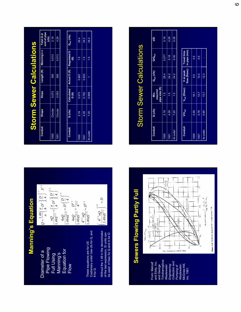
Storm

Sewer Calculations

4.29

0.013

300

0.053

Circular

1001

2.19

0.013

300

0.073

Circular

1000

Total Q at

end of pipe

(cfs)

Manning’s n

Length (ft)

Slope

Shape

Conduit

24.2

1.5

10.958

7.25

At outlet

24.2

1.5

0.833

0.792

4.29

1001

28.4

1.5

0.667

0.573

2.19

1000

Qfull(cfs)

Regulated D

(ft)

Actual D (ft)

Calculated

D (ft)

Q (cfs)

Conduit

Sewers Flowing Partly Full

From: Metcalf

and Eddy, Inc.

and George

Tchobanoglous.

Wastewater

Engineering:

Collection and

Pumping of

Wastewater.

McGraw-Hill,

Inc. 1981.

Storm

Sewer Calculations

0.38

0.30

24.2

1.5

7.25

At outlet

0.29

0.18

24.2

1.5

4.29

1001

0.19

0.077

28.4

1.5

2.19

1000

d/D

Q/Q

full

Qfull(cfs)

Min.

required

pipe size (ft)

Q (cfs)

Conduit

12.3

10.4

9.5

V at peak

flow (ft/sec)

-13.7

0.90

At outlet

0.5

13.7

0.76

1001

0.5

16.1

0.59

1000

Travel time

in pipe (min)

Vfull(ft/sec)

V/V

full

Conduit

7

Pipe Sizes

•Minimum size 12 -18 inches

•In m

any locations, the m

inimum size of a

storm

sewer pipe is regulated

Velocities

•Minimum velocity of 2.0 ft/sec (0.6 m/sec)

with flow at ½

full or full depth

•Maximum average velocities of 10-12

ft/sec (2.5-3.0 m/sec) at design depth of

flow

•Minimum and m

aximum velocities m

ay be

specified in state and local standards

Slopes

•Sewers with flat slopes may be required to avoid

excessive excavation where surface slopes are

flat or the changes in elevation are small.

•In such cases, the sewer sizes and slopes

should be designed so that the velocity of flow

will increase progressively, or at least will be

steady throughout the length of the sewer.

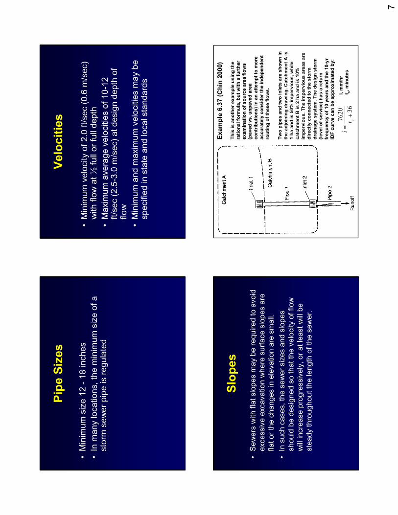
Example 6.37 (Chin 2000)

This is another example using the

rational form

ula, but with a further

examination of source area flows

(paved vs. unpaved area

contributions) in an attempt to m

ore

accurately consider the independent

routing of these flows.

Two pipes and two inlets are shown in

the adjoining drawing. Catchment A is

1 ha and is 50% impervious, while

catchment B is 2 ha and is 10%

impervious. The impervious areas are

directly connected to the storm

drainage system. The design storm

(level of service) has a return

frequency of 10 years and the 10-yr

IDF curve can be approxim

ated by:

i, m

m/hr

t c, minutes

36

7620

+=

cti

8

Basic watershed data:

The effective rainfall rate (i e) is as follows, using the IDF curve equation and

the rational form

ula:

36

7620

+=

=c

et

CCi

iwhere C is the runoff coefficient. The tim

e of

concentration can be estimated using the

following equation:

()

3.0 0

4.0

6.0

99

.6

SinL

te

c=

Where n is the M

anning’s roughness factor for

sheetflow conditions, L is the flow length (m)

and S

ois the slope of the watershed, as

presented in the above data table.

These equations are solved sim

ultaneously to obtain the following tim

e of

concentration values for each watershed subarea:

Flows at Inlet 1 and Pipe 1:

Pipe 1 only receives runoff from inlet 1, contributed by catchment A. When

the entire catchment A is contributing flow, the tim

e of concentration is 46

minutes (the tim

e needed for both the pervious and impervious areas to be

fully contributing). The average rainfall rate corresponding to this tim

e of

concentration is therefore 92.9 m

m/hr (or 2.58 x 10-5m/sec). The area-

weighted runoff coefficient is:

()

()

55

.0

2.0

5.0

9.0

5.0

=+

=C

Since the area of the catchment is 1 ha (10,000 m

2), the peak runoff rate,

Qp, can be calculated using the rational form

ula as:

()(

)()

sm

ms

mx

iAC

Qp

/142

.0

000

,10

/10

58

.2

55

.0

32

5=

==

−

However, the impervious area should be examined alone, as it may

produce a greater peak flow rate than the whole averaged area. This

recognizes the separate routing of flows from these greatly different

subareas. The tim

e of concentration of the impervious area in catchment A

is 11 m

inutes, and the corresponding rainfall rate averaged for that

duration is 162 m

m/hr (4.5 x 10-5m/sec). The impervious area runoff

coefficient is 0.9 and the area is 0.5 ha (5,000 m

2). Therefore, the peak

runoff rate, Q

p, can be calculated as:

()(

)()

sm

ms

mx

iAC

Qp

/203

.0

000

,5

/10

50

.4

9.0

32

5=

==

−

This calculated peak runoff rate for the impervious areas alone is therefore

greater than the peak runoff rate calculated for the whole catchment

averaged conditions, and is therefore controlling. The flow to be handled in

Pipe 1 is therefore 0.203 m

3/sec.

Flows at Inlet 2:

When the entire catchment B is contributing flow, the inlet timeof

concentration is 71 m

inutes. The corresponding averaged rainfallrate for

this duration is 71.2 m

m/hr (1.98 x 10-5m/sec) and the area-w

eighted runoff

coefficient is:

()

()

27

.02.0

9.09.0

1.0=

+=

C

The catchment B area is 2 ha (20,000 m

2) and the peak runoff rate is therefore:

()(

)()

sm

ms

mx

iAC

Qp

/107

.0

000

,20

/10

98

.1

27

.0

32

5=

==

−

The impervious area alone has a tim

e of concentration of 12 m

inutes, and

the corresponding averaged rainfall rate for that period is 159 m

m/hr (4.41 x

10-5m/sec). The impervious area runoff coefficient is 0.9 and the area is 0.2

ha (2,000 m

2). The peak runoff rate just from the impervious area component

of catchment B is therefore:

() (

)()

sm

ms

mx

iAC

Qp

/079

.0

000

,2

/10

41

.4

9.0

32

5=

==

−

In this case, the peak flow is greater when the whole catchment conditions

are averaged, and the peak flow at inlet 2 is therefore 0.107 m

3/sec.

9

Flow in Pipe 2:

The peak flow for pipe 2 m

ust consider several alternatives. Thefirst case

considers the entire 3 ha (30,000 m

2) area of catchments A plus B averaged

together (a common way of applying the rational form

ula, as previously

illustrated). The tim

e of concentration for catchment A contributions is the

inlet time of concentration of 46 m

in., plus the travel time of the flow in pipe

1, here assumed to be 2 m

in. This potential time of travel path therefore totals

48 m

inutes. This is compared to the inlet time of concentration of catchment

B which is 71 m

in. The 71 m

in. pathway is therefore the longest and is the

time of concentration. The corresponding rainfall rate averaged for this

period is 71.2 m

m/hr (1.98 x 10-5m/sec). The area-w

eighted runoff coefficient

is therefore:

()(

)(

)()

[]

36

.0

2.0

8.1

5.0

9.0

2.0

5.0

31=

++

+=

C

and the peak runoff rate is calculated as:

()(

)()

sm

ms

mx

iAC

Qp

/214

.0

000

,30

/10

98

.1

36

.0

32

5=

==

−

Considering the impervious areas of catchments A and B alone, the area

is 0.7 ha (7,000 m

2) and the tim

e of concentration is 13 m

in. (the 11 m

in.

time of conc. for the impervious areas in catchment A plus the 2min.

travel time in Pipe 1 vs. the 12 m

in. time of concentration for the

impervious areas in catchment B). The corresponding rainfall rate

averaged for this tim

e is 156 m

m/hr (4.32 x 10-5m/sec), the runoff

coefficient is 0.9, and the rational form

ula provides the peak runoff rate:

() (

)()

sm

ms

mx

iAC

Qp

/272

.0

000

,7

/10

32

.4

9.0

32

5=

==

−

Therefore, the peak flows using the impervious areas alone are

controlling for Pipe 2.

In reality, it is likely that the m

ost critical condition would be

associated with a combination of conditions, possibly using the

impervious area data from catchment A and the entire area from

catchment B. It is not easy to tell unless a complete hydrograph

routing m

ethod that examines the separate subareas is used, suchas

WinTR-55 for the m

ajor drainage areas (or surface drainage), or

SWMM5 for any condition. Recall that with W

inTR-55, it is necessary

to separate subcatchments that differ by a CN of 5, or greater, in each

subwatershed.

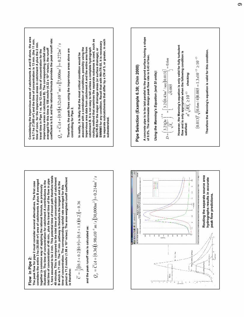
Routing the separate source area

hydrographs results in accurate

peak flow predictions.

Pipe Selection (Example 6.38; Chin 2000)

A concrete pipe is to be laid parallel to the ground surface having a slope

of 0.5%. The storm

water design peak flow rate is 0.43 m

3/sec.

Using the Manning’s Equation (and SI units):

()(

)m

m

SQn

Do

6.0

005

.0

013

.0

sec

/43

.0

21

.3

21

.3

38/

3

=

=

= However, the M

anning’s equation is only valid for fully turbulent

flow and is only appropriate when the following condition is

satisfied:

13

610−

≥o

RS

n

()

()

13

13

610

10

3.1

005

.0

4/6.

0013

.0

−−

≥=

xm

checking:

Therefore the M

anning’s equation is valid for this condition.

10

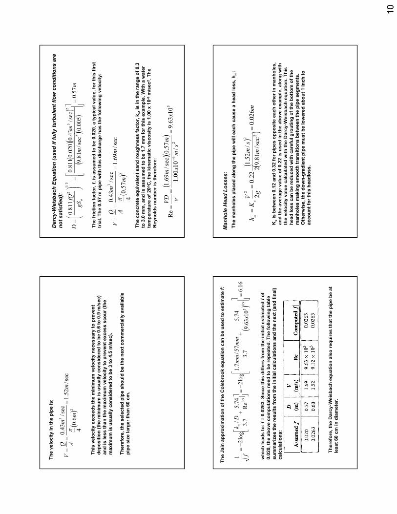
The velocity in the pipe is:

()

sec

/52

.1

6.0

4

sec

/43

.0

2

3

m

m

m

AQV

==

=π

This velocity exceeds the m

inim

um velocity necessary to prevent

deposition (the m

inim

um is usually considered to be 0.6 to 0.9 m

/sec)

and is less than the m

axim

um velocity to prevent excess scour (the

maxim

um is usually considered to be 3 to 4.5 m

/sec).

Therefore, the selected pipe should be the next commercially available

pipe size larger than 60 cm.

Darcy-Weisbach Equation (used if fully turbulent flow conditions are

not satisfied):

()(

)(

)()

mm

m

gS

fQD

o

57

.0

005

.0

sec

/81

.9

sec

/43

.0

020

.0

811

.0

811

.0

2

23

5/1

2

=

=

=

The friction factor, f, is assumed to be 0.020, a typical value, for this first

trial. The 0.57 m

pipe with this discharge has the following velocity:

()

sec

/69

.1

57

.0

4

sec

/43

.0

2

3

m

m

m

AQV

==

=π

The concrete equivalent sand roughness factor, k

s, is in the range of 0.3

to 3.0 m

m, and is assumed to be 1.7 m

m for this example. With a water

temperature of 20oC, the kinematic viscosity is 1.00 x 10-6m/sec2. The

Reynolds number is therefore:

()(

)5

26

10

63

.9

/10

00

.1

57

.0

sec

/69

.1

Re

xs

mx

mm

VD

==

=−

ν

The Jain approxim

ation of the Colebrook equation can be used to estimate f:

()

16

.6

10

63

.9

74

.5

7.3

57

/7.

1log

2Re74

.5

7.3

/log

21

9.0

59.

0=

+

−=

+−

=x

mm

mm

Dk

f

s

which leads to: f= 0.0263. Since this differs from the initial estimated fof

0.020, the above computations need to be repeated. The followingtable

summarizes the results from the initial calculations and the next (and final)

calculations:

Therefore, the Darcy-W

eisbach equation also requires that the pipe be at

least 60 cm in diameter.

Manhole Head Losses:

The m

anholes placed along the pipe will each cause a head loss, hm:

()

()

mm

sm

g

VK

hc

m026

.0

sec

/81

.9

2

/52

.1

22

.0

22

22

==

=

Kcis betw

een 0.12 and 0.32 for pipes opposite each other in m

anholes,

and the average value of 0.22 is used in the above example, along with

the velocity value calculated with the Darcy-W

eisbach equation. This

head loss can be reduced with careful grouting of the bottom of the

manholes m

aking smooth transitions betw

een the pipe segments.

Otherw

ise, the down-gradient pipe m

ust be lowered about 1 inch to

account for this headloss.

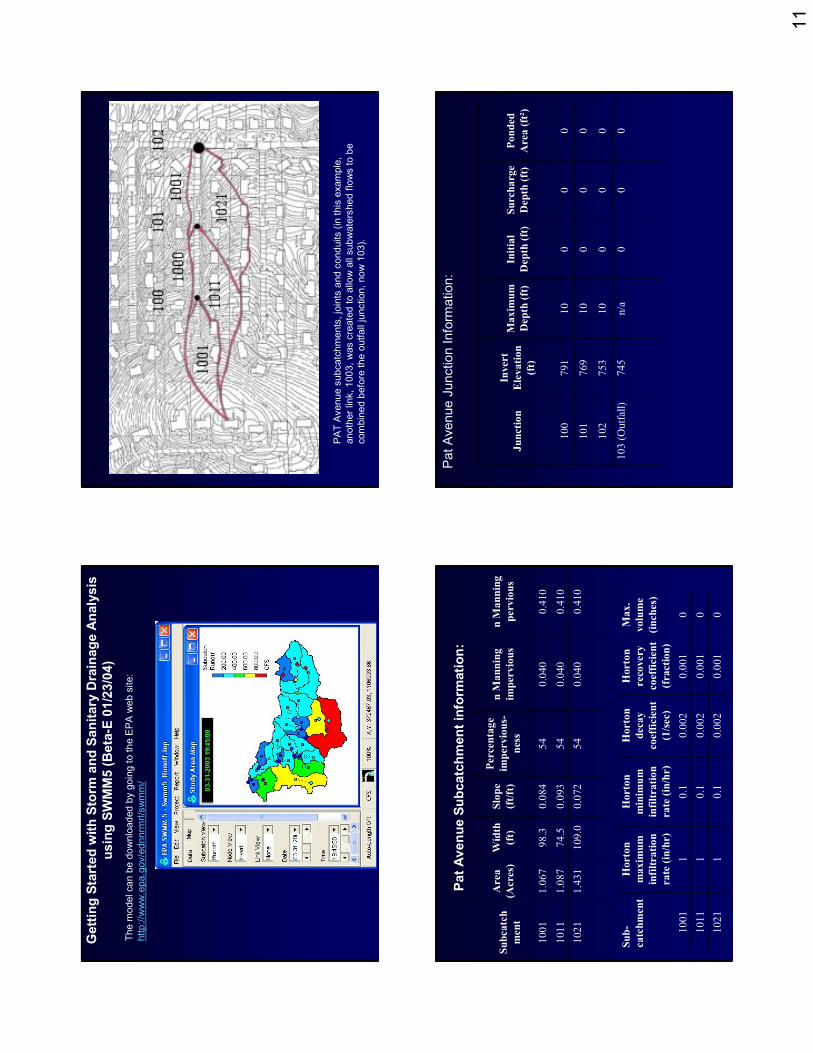
11

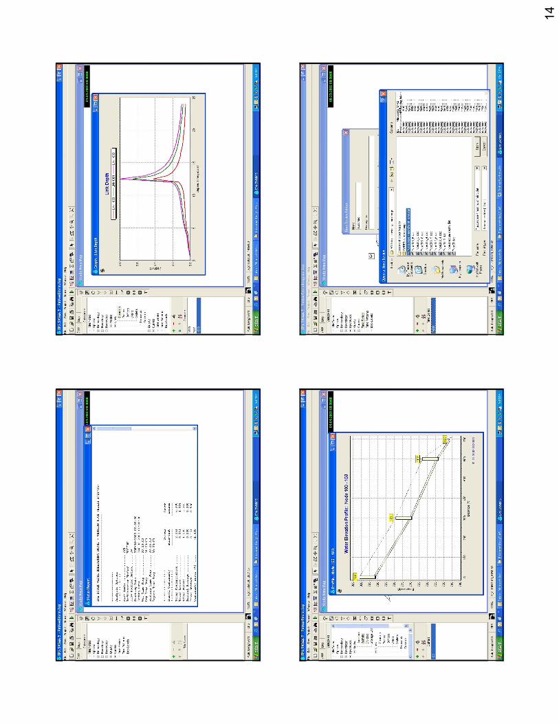
Getting Started with Storm

and Sanitary Drainage Analysis

using SWMM5 (Beta-E 01/23/04)

The model can be downloaded by going to the EPA web site:

http://www.epa.gov/ednnrm

rl/swmm/

PAT Avenue subcatchments, joints and conduits (in this example,

another link, 1003, was created to allow all subwatershed flows to be

combined before the outfall junction, now 103).

Pat Avenue Subcatchment inform

ation:

0.410

0.040

54

0.072

109.0

1.431

1021

0.410

0.040

54

0.093

74.5

1.087

1011

0.410

0.040

54

0.084

98.3

1.067

1001

n M

annin

g

pervio

us

n M

annin

g

impervio

us

Perce

nta

ge

impervio

us-

ness

Slo

pe

(ft/

ft)

Wid

th

(ft)

Area

(Acre

s)Subcatc

h

ment

00.001

0.002

0.1

11021

00.001

0.002

0.1

11011

00.001

0.002

0.1

11001

Max.

volu

me

(inches)

Horto

n

reco

very

coef

ficie

nt

(fracti

on)

Horto

n

decay

coef

ficie

nt

(1/s

ec)

Horto

n

min

imum

infi

ltrati

on

rate

(in

/hr)

Horto

n

maxim

um

infi

ltrati

on

rate

(in

/hr)

Sub-

catc

hm

ent

Pat Avenue Junction Inform

ation:

00

0n/a

745

103 (Outfall)

00

010

753

102

00

010

769

101

00

010

791

100

Ponded

Area (

ft²)

Surcharge

Depth

(ft

)

Init

ial

Depth

(ft

)

Maxim

um

Depth

(ft

)

Invert

Ele

vati

on

(ft)

Juncti

on

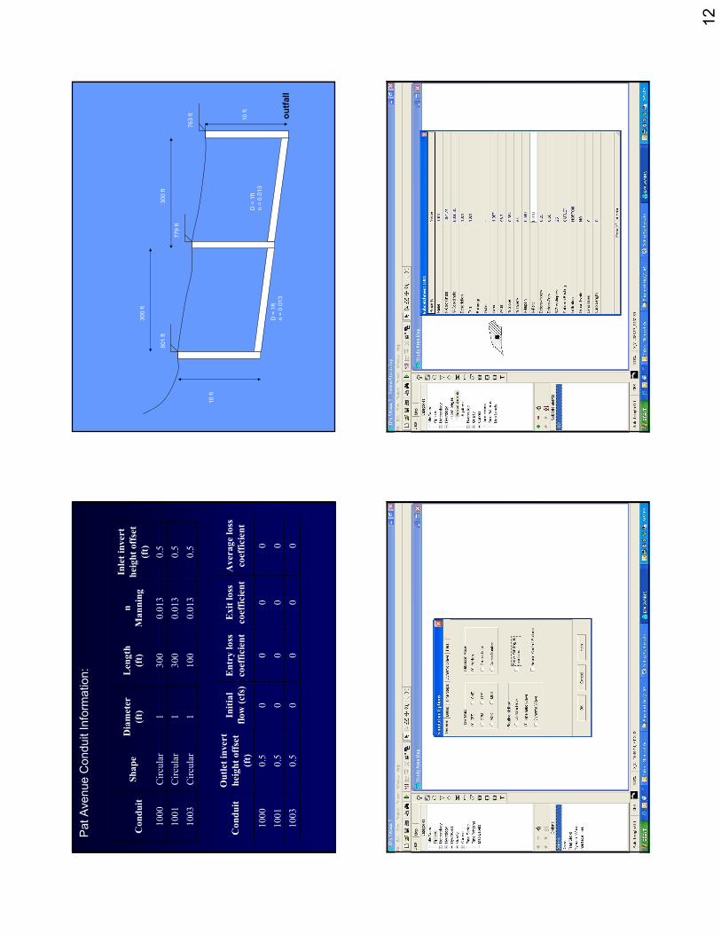
12

Pat Avenue Conduit Inform

ation:

0.5

0.013

100

1Circular

1003

0.5

0.013

300

1Circular

1001

0.5

0.013

300

1Circular

1000

Inle

t in

vert

heig

ht

off

set

(ft)

n

Mannin

g

Length

(ft)

Dia

mete

r

(ft)

Shape

Conduit

00

00

0.5

1003

00

00

0.5

1001

00

00

0.5

1000

Average loss

coef

ficie

nt

Exit

loss

coef

ficie

nt

Entr

y loss

coef

ficie

nt

Init

ial

flow

(cf

s)

Outl

et

invert

heig

ht

off

set

(ft)

Conduit

801 ft

779 ft

763 ft

10 ft

10 ft

300 ft

300 ft

D = 1ft

n = 0.013

D = 1ft

n = 0.013

outfall

13

14

15

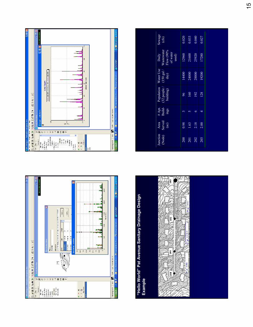
“Hello W

orld”Pat Avenue Sanitary Drainage Design

Example

0.027

17280

19200

128

42.00

203

0.040

25920

28800

192

62.18

202

0.033

21600

24000

160

51.63

201

0.020

12960

14400

96

30.98

200

Sew

age

(cfs)

Daily

Wastewater

Flow (90%

of water

used)

Water Use

(150 gal /

day)

Population

(32 people /

building)

# Apt.

Build-

ings

Area

Served

(ac)

Junction

(Node)

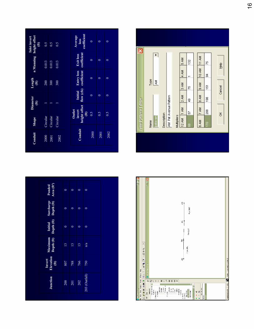
16

00

0n/a

750

203 (Outfall)

00

013

766

202

00

013

788

201

00

013

807

200

Ponded

Area (

ft²)

Surcharge

Depth

(ft

)

Init

ial

Depth

(ft

)

Maxim

um

Depth

(ft

)

Invert

Ele

vati

on

(ft)

Juncti

on

0.5

0.013

300

1Circular

2002

0.5

0.013

300

1Circular

2001

0.5

0.013

200

1Circular

2000

Inle

t in

vert

heig

ht

off

set

(ft)

n M

annin

gL

ength

(ft)

Dia

mete

r

(ft)

Shape

Conduit

00

00

0.5

2002

00

00

0.5

2001

00

00

0.5

2000

Average

loss

coef

ficie

nt

Exit

loss

coef

ficie

nt

Entr

y loss

coef

ficie

nt

Init

ial

flow

(cf

s)

Outl

et

invert

heig

ht

off

set

(ft)

Conduit

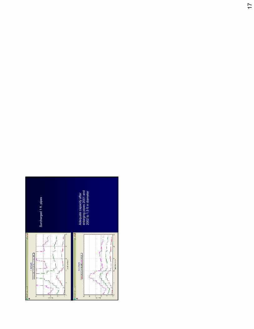
17

Surcharged 1 ft. pipes

Adequate capacity after

enlarging pipes 2001 and

2002 to 1.5 ft in diameter