SEDIMENT TRANSPORT MODEL FOR STORM SEWER...

47

RiscuRi şi catastRofe, an Xv, vol. 19, nR. 2/2016

SEDIMENT TRANSPORT MODEL FOR STORM SEWER NETWORKS TOWARDS THE

OPERATIONAL RISKS

I. RÁTKY1, M. KNOLMÁR2

AbSTRACT.- Sediment Transport Model For Storm Sewer Networks To wards the Operational Risks.Sediment transport in sewer networks can be crit-ical in economical and safety point of view. To improve the operation of the sewer networks we are presenting a model, which is capable of numerical simulations of the sediment transport in storm water network. The developed model is calculating the change of the particle distribution of the sediment fractions including the ef-fects of settling and mixing up processes. The results of the model calculations in a simplified network are also presented. We are also planning to apply the developed sediment transport module by coupling to a hydrodynamic simulation for practical tasks supporting the design and operation of sewers networks.

Key-words: sediment transport, storm water network, hydrodynamic simulation, sewer design and operation

1. INTRODUCTION

It is hard to state whether the demand for sustainable development including the environmental protection forces the technical development or on the contrary, the state of the development e.g. the information technology dictates the demand for the sustainment. The question is similar to the chicken or the egg causality. Instead of theories, there is a wide agreement, that the state of the development in the science and technology is attaching to the social demand i.e. the sustainable development, they are catalysing each other. The engineers should “just” use their scientific and technical knowledges for serving the social demands. They should also show how to apply the already developed technical possibilities for the satisfaction of the social demands. Theoretical and computer technical knowledge proved useful on other fields are applicable for storm sewers design in order to improve the operation of the sewer networks in economical and safety point of view. Our special target was to develop a model, which is capable of numerical simulations of the sediment transport in storm water network and presenting the results of the model calculations in a simplified network.

1 Budapest University of Technology and Economics, Hungary, E-mail: [email protected] [email protected]

48

I. Rátky, M. knolMáR

Our long scale target is to build and present the practical application of the developed sediment module into a computer program supporting the designing and operational tasks. An author of this article preparing his PhD thesis (Knolmár 2011) had already made the first steps toward this goal.

The cited thesis presented a general overview of the international and Hungarian publications regarding the current scope. We are only summarizing here the important features of the most popular program packages calculating the sediment transport of the storm sewers closely related to our developments (Knolmár 2011):

• The SWMM (Storm Water Management Model) hydrologic-hydrau-lic-water quality simulation model is a worldwide used program developed by the US EPA. The early versions from 1973 (Extended Transport Block - EXTRAN) (Roesner et al. 1992) were including calculations for suspended solid sediment trans-port, but this versions were not available for public access. The program has been un-der a continuous revision and development, but the developer stopped the sediment transport development. Later the EPA completely excluded the sediment transport module from the program (Fan et al. 2003). In the newer versions of SWMM (Ross-man 2010) the sediment transport is still not included and the development of EPA is not aiming this area.

• In the Danish developed DHI Mouse sewer simulation program, the user can select the most applicable sediment transport model from the built-in ones for the current conditions. The user can form the models flexible by the parameter set-ting. The calculation of different morphological changes like sedimentation, erosion, dunes are selectable. The effect of the bottom changes on the sediment transport and the adhesive processes can be included. However, the user interface and the user manual are not supporting sufficiently the parameter settings of the transport models. The good knowledge about the original models is necessary for the built-in models. The Mike Urban program (DHI 2009) operating on GIS structures proved a bit uneasy, overcomplicated during intensive usage. Besides the advantages given by the GIS structures, this program is showing the typical disadvantages of the closed-source commercial software products.

• In the InfoWorks CS hydrodynamic simulation package (Wallingford 2010) developed by the Wallingford Software UK company it is possible to select from several sediment transport model. The morphological changes are included, but some important parameters and initial conditions are not possible to set by the user demands (Mannina et al. 2012).

• The US developed XP Software XPSWMM package is including several new functions compared to the original SWMM and these are available through its modern user interface. The sediment transport calculation is a simplified solution, there is no distinction between the suspended and bed load forms, morphological changes are not included, but there are fractions of particles.

49

Sediment tranSport model For Storm Sewer networkS towardS the operational riSkS

The most of the above listed models are commercial products, the rest are research and development tools. The acquisition costs of the commercial programs are usually high. The supporting services like upgrade, consultancy are usually not free. The drivers of development and upgrade are often commercial considerations instead of the technical demands. The user is at the mercy of the developing company. The source code is not open, the calculation algorithms are usually unknown and not variable (black box).

This short and schematic review of the models is showing that it is a promising task to start a development from an existing open source hydrodynamic program and to expand its capabilities with morphological computations fitted to the local demands like data availability, designing and operational rules.

2. MODEL bUILDING ASPECTS AND APPROXIMATIONS

In order to calculate the routing of the solid materials getting into the sewer network with acceptable accuracy we should try to understand the hydraulic and sediment transport processes like settling, mixing up and flushing out.

The mathematical description of the phenomena is approximated first with a one-dimensional (1D) model. Only after the understanding of the phenomena can we decide about the applicability of the 1D model. It is impossible to review all known and general demands on the mathematical and numerical models e.g. to provide a solution supporting design and operation, giving acceptable accuracy and hardware demand. We highlight only three quite important model-building criteria here:

i. simplicity of the modelii. availability of necessary data

iii. calibration possibilities, the availability of required measured data

Selecting 1D model is satisfying the first criterion. However there could be different approximations like several calculation segments inside the conduit section (i.e. the branch between two junctions) or to take the conduit section as one calculation segment. If we characterize the sediment by just one or two quantities like one concentration or one particle diameter inside the calculation segment, then the calculation is 1D in point of view of the sediment. If there are different typical particle diameters for the bed load and for the suspended load and both of them have variable particle size fractions, then that is not a typical 1D-calculation method of sediment transport.

Fluid flow with solid transport in closed or open channels (free water surface i.e. not under pressure) is only slightly differing from the open channel river flow processes regarding their basics. Presently, in the point of view of the model building the most important differences are:

50


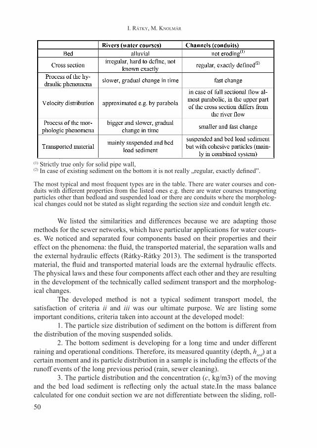
(1) Strictly true only for solid pipe wall, (2) In case of existing sediment on the bottom it is not really „regular, exactly defined”.

The most typical and most frequent types are in the table. There are water courses and con-duits with different properties from the listed ones e.g. there are water courses transporting particles other than bedload and suspended load or there are conduits where the morpholog-ical changes could not be stated as slight regarding the section size and conduit length etc.

We listed the similarities and differences because we are adapting those methods for the sewer networks, which have particular applications for water cours-es. We noticed and separated four components based on their properties and their effect on the phenomena: the fluid, the transported material, the separation walls and the external hydraulic effects (Rátky-Rátky 2013). The sediment is the transported material, the fluid and transported material loads are the external hydraulic effects. The physical laws and these four components affect each other and they are resulting in the development of the technically called sediment transport and the morpholog-ical changes.

The developed method is not a typical sediment transport model, the satisfaction of criteria ii and iii was our ultimate purpose. We are listing some important conditions, criteria taken into account at the developed model:

1. The particle size distribution of sediment on the bottom is different from the distribution of the moving suspended solids.

2. The bottom sediment is developing for a long time and under different raining and operational conditions. Therefore, its measured quantity (depth, hsed) at a certain moment and its particle distribution in a sample is including the effects of the runoff events of the long previous period (rain, sewer cleaning).

3. The particle distribution and the concentration (c, kg/m3) of the moving and the bed load sediment is reflecting only the actual state.In the mass balance calculated for one conduit section we are not differentiate between the sliding, roll-

51


ing, jumping particles on the bottom and the suspended solids moving continuously above them. We are assuming that both types are “going” to the next calculation seg-ment in one dt time step, i.e. the time and conduit length are enough for the settling and for the total mixing up.

4. It is hard to imagine that the model can be calibrated based on the infre-quently taken samples. There are several problems:

- The past runoff and operational conditions are not known, nor the hy-draulic load on selected conduit sections, Qi(t) and cu(t)

- Similar problem is originating from the knowledge of the temporal change of the cumulatively settled sediment hsed,i(t), (cm) or Mb,i(t), (kg), its concen-tration, cb(t), its density ρw, (kg/m3) and its particle distribution.

- Even if the values of Qi(t) are known, but the past quantities of cu(t), hsed,i(t), Mu(t) and the particle distribution are not measured continuously, therefore these parameters can be calculated (estimated) by the model for the whole system (when this model is not yet calibrated).

5. Neither the external hydraulic effects nor the data resulting from them are available now at the frequency and accuracy satisfying the calibration demand of the model.

6. The problems described in point 5 and 6 should not result in neglect of the concentration and particle distribution differences of the transported and settled sediment, because probably it is not possible to calibrate them in the model. The inclusion of existing real parameters in the processes and their differences even with estimated values are giving certainly better result than without them. It is also high-lighting the importance of the improvement of the model accuracy and its calibration.

3. DATA REQUIREMENTS OF THE CALCULATIONS

3.1. Geometrical DataDi – main geometric parameter of the conduit section (i), in general the

diameter, (Conduit section: the length of conduit having identical main geometric size

or conduit between two manholes or inflow-outflow structure),Li – length of conduit section,dxi – section length of calculation, can be determined by the average (min or

max) flow velocities developing during the whole calculation time interval.ho,i – the sediment depth on the bottom at the start of calculation, (Maximum of the settled sediment depth).

3.2. Hydraulic Dataλi – pipe friction parameter of conduit section (equivalent friction parameter), Initial conditions:

52


Qo,i – initial flows at the start of the calculation, constant for a conduit section, variable at section borders, but always increasing downwards (not calculating with surface floods now).

Upper and lateral boundary conditions:Qi(t) – flows loading the system, variable for conduit sections and in time

– increasing downwards. Lower boundary conditions: As everywhere, at the lowest calculation segment we are assuming a

convective fluid mass transport, therefore additional flow and water depth/head values are not necessary to define.

3.3. Sediment and Morphologic Data:ρd and ρw, (kg/m3) – density of dry sediment and density of sediment under

water (w). Initial conditions: For each conduit section (i):– concentration of the suspended solid (co,i, kg/m3), (in all points of all con-

duit sections of the given system at the first moment of the calculation), – the particle size distribution of the suspended solid, (d1,t-p1,t d2,t-p2,t, …

,dn,t-pn,t)t=0,– the initial depth of the settled sediment on the bottom (ho,i), from which

the settled volume can be calculated for each segment in case of known section sizes and densities, Mb,i (kg),

– the particle size distribution of the settled sediment on the bottom, (d1,b-p1,b, d2,b-p2,b,…,dn,b-pn,b)t=0.

Now and also below the lower index t is abbreviation for transported ma-terial and lower index b is for the material on the bottom, the lower index i for the calculation segment, the lower index j is for the actual fraction.

Upper boundary conditions:– The concentration of the suspended solid (co,i, kg/m3) loading the system,

changing in time (suspended solid concentration of the flow reaching the upper con-duit section), cub(t).

– The particle size distribution of the arriving sediment (d1,ub-p1,fh d2,ub-p2,ub, … , dn,ub-pn,ub)t=0→T. It is constant in the current development level of the model.

Lower boundary condition: – Assuming that the dispersive transport is negligible at the lowest conduit

segment (as everywhere) compared to the convective one, lower boundary condition is not necessary to give for sediment.

53


4. ALGORITHMIC STEPS OF THE MORPHOLOGICALCALCULATION

4.1. Determination of the Segment LengthThe length of the calculation segments (dxi) for the assumed convective

water and mass transport are determined based on the flow velocities (vi) developing in the conduit sections and the calculation time steps (dt). We can calculate the velocities for the conduit sections from the given upper and lateral flow loads and the geometric data. The calculation of dxi was done at the time of t = 0, this time during the calculation of velocities (vi) there was zero settled sediment assumed. We could calculate the velocities (vi) and the calculation lengths (dxi) of a segment from the minimum, average or the maximum flow in the model during the whole calculation time interval. One conduit section is usually divided into several dx. Then all calculations are regarding for the dx segment length.

We execute the sediment transport calculations – settling and mixing up – separately for the typical particle distribution fraction diameters dj,t and dj,b for the transported and for the settled sediment on the bottom. We assumed that these two processes are not influencing each other. For each particle diameter, we calculate the mass as settling or mixing up. The result is showing, that the transported or settled mass on the bottom belonging to a given particle diameter is increasing or decreasing depending on the type of the resulting process (settling or mixing up). After the calculations for all the dj the new particle distribution is determined based on the plus/minus mass change for each dj.

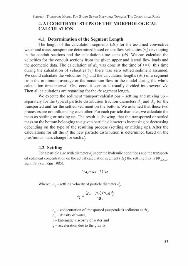
4.2. SettlingFor a particle size with diameter dj under the hydraulic conditions and the transport-

ed sediment concentration on the actual calculation segment (dxi) the settling flux is (Φdj,down, kg/m2/s) (van Rijn 1985):

Where: ωj – settling velocity of particle diameter dj,

ci,t – concentration of transported (suspended) sediment at dxi, ρw – density of water, ν – kinematic viscosity of water and g – acceleration due to the gravity.

54


The settled sediment mass in the dxi calculation segment, having diameter fraction dj, during time interval dt is:

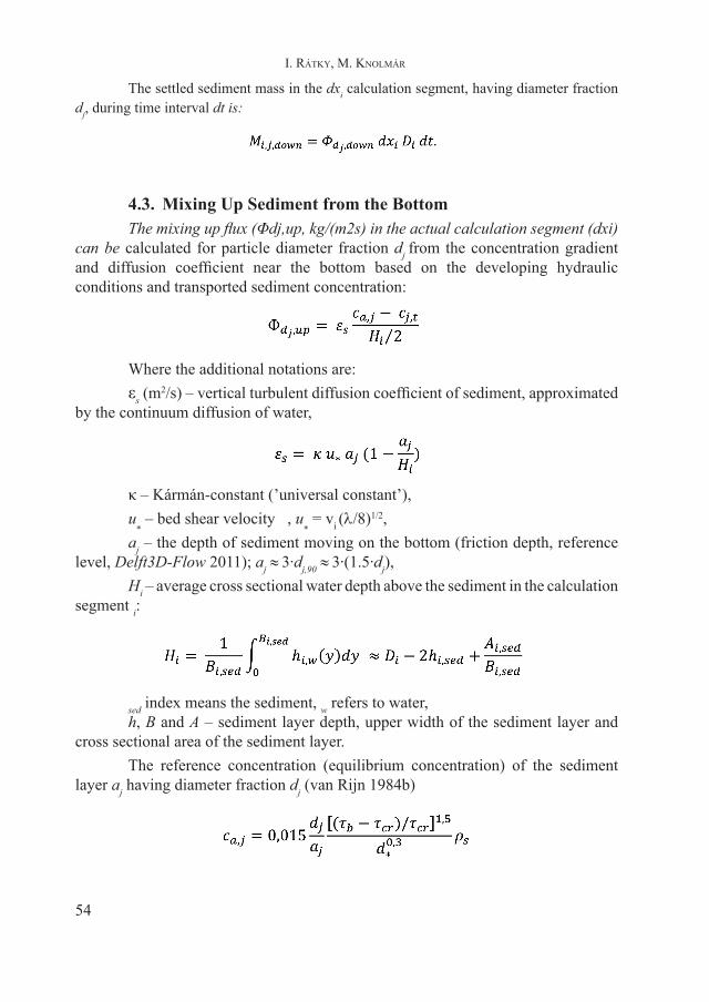
4.3. Mixing Up Sediment from the bottomThe mixing up flux (Φdj,up, kg/(m2s) in the actual calculation segment (dxi)

can be calculated for particle diameter fraction dj from the concentration gradient and diffusion coefficient near the bottom based on the developing hydraulic conditions and transported sediment concentration:

Where the additional notations are:εs (m

2/s) – vertical turbulent diffusion coefficient of sediment, approximated by the continuum diffusion of water,

κ – Kármán-constant (’universal constant’),u

* – bed shear velocity , u

* = vi (λ/8)1/2,

aj – the depth of sediment moving on the bottom (friction depth, reference level, Delft3D-Flow 2011); aj ≈ 3∙dj,90 ≈ 3∙(1.5∙dj),

Hi – average cross sectional water depth above the sediment in the calculation segment i:

sed index means the sediment, w refers to water, h, B and A – sediment layer depth, upper width of the sediment layer and

cross sectional area of the sediment layer. The reference concentration (equilibrium concentration) of the sediment

layer aj having diameter fraction dj (van Rijn 1984b)

55


where:τ

b – bed shear stress of bottom, τ

b = ρw∙u

*2,

τcr – critical bed shear stress, using the analytical approximation of the

transport stage parameter (analytical form of the Shields-curve, van Rijn 1984a, DHI 2008), now in case of d* ≤ 4:

d* – dimensionless particle diameter

∆ = ρs/ρw-1.

The mixed up sediment mass in the dxi calculation segment, having diameter fraction dj, during time interval dt is:

4.4. Calculation of morphologic changeBoth of the Mi,j,down and Mi,j,up were so far potential settling down or mixing

up mass. Nevertheless, it is not sure that the mass in the segment dxi (coming from the upper segment) is containing as much mass from the fraction of dj as calculated (Mi,j,down). It is also not sure that there is as much mass on the bottom from the fraction of dj as should be mixed up based on the calculated Mi,j,up. That is why these calculated masses are potential. In short: the settling mass of any fraction is limited by the suspended mass in the segment, and the mixing up mass is limited by the sediment on the bottom. Regarding these limitations and assuming these processes as independent from each other, we can determine the effective settling and mixing up mass for each fraction. The result of these two processes – calculating by fractions and regarding their sign expressing the direction of the movement – can be mixing up, settling or balance (when the potential mixing is exactly equal to the settling). The sediment on the bottom and the transported (suspended) total mass can be determined regarding the described possibilities and executing the sum for each fraction. The transported and settled sediment concentration, the settled sediment volume and the sediment depth (hi,sed) can be calculated for the segment dxi and for the moment t+dt based on the total mass change during one time interval (dt). Based

56


on the resulting mass for each fraction the distribution of the transported (dj,t–pj,t) and settled sediment (dj,b –pj,b) can be determined for the moment t+dt too.

Summarized: For the calculation segment dxi for an event after a dt time step (t+dt) transporting Qi flow, there are available the following quantities:

Concentration of the suspended sediment ci,t, mass flow (ci,t∙Qi), particle distribution of the transported sediment (dj,t–pj,t), depth (hi,sed), volume, total mass (Mb) and particle distribution of the sediment on the bottom (dj,b–pj,b).

Based on the sediment volume on the bottom we can calculate the flow velocity vi, which is determining hydraulic conditions of the settling and mixing up for the next dt time interval.

5. DEMONSTRATION OF OPERAbILITy OF THE ALGORITHM

Our long term target is to build the developed algorithm into such a software like SWMM or EPANET, which can calculate the hydraulic processes existing in any type (combined or separated, gravitational or pressurized) of sewer system. As we emphasized previously „Modelling of the sediment transport can significantly help to select the optimal operational intervention in case of the extension or reconstruction of the existing sewer networks.” (Knolmár 2011). Building the sediment transport module into an existing hydraulic program still means a quite hard work, therefore before that kind of development, it is worth trying the operation of the model in a simple network. In this section, we demonstrate the operation of a pressurized conduit system consisting of some short sections without loops and dividers.

5.1. Geometric Data and Constant Parameters of the Sediment Load

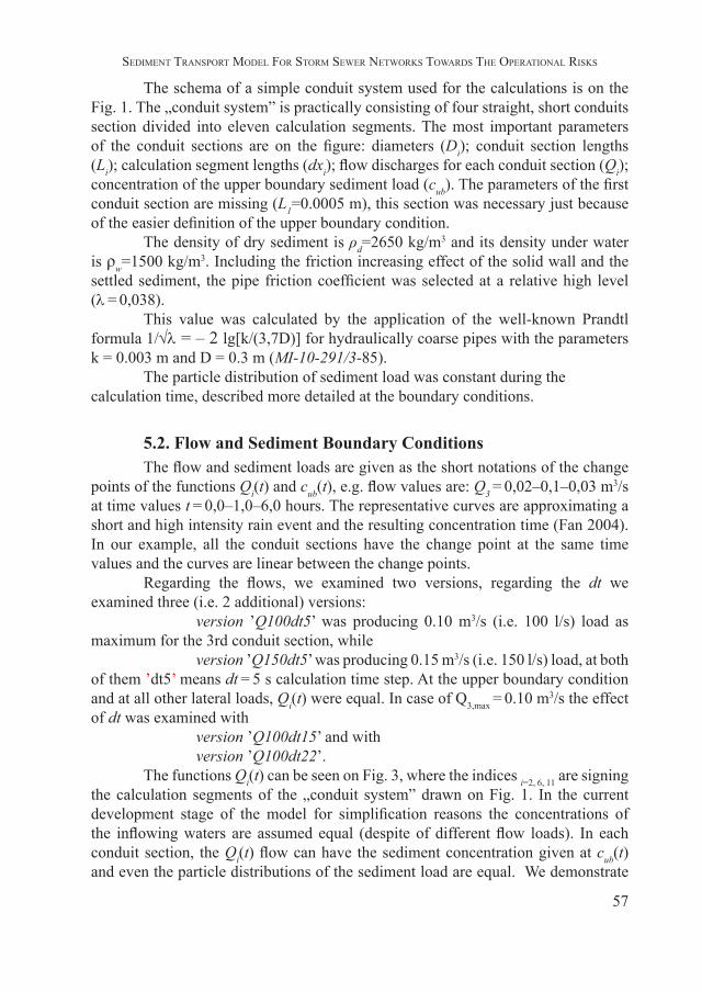
Figure 1. The schema of the “conduite system” applied for the calculation

57


The schema of a simple conduit system used for the calculations is on the Fig. 1. The „conduit system” is practically consisting of four straight, short conduits section divided into eleven calculation segments. The most important parameters of the conduit sections are on the figure: diameters (Di); conduit section lengths (Li); calculation segment lengths (dxi); flow discharges for each conduit section (Qi); concentration of the upper boundary sediment load (cub). The parameters of the first conduit section are missing (L1=0.0005 m), this section was necessary just because of the easier definition of the upper boundary condition.

The density of dry sediment is ρd=2650 kg/m3 and its density under water is ρw=1500 kg/m3. Including the friction increasing effect of the solid wall and the settled sediment, the pipe friction coefficient was selected at a relative high level (λ = 0,038).

This value was calculated by the application of the well-known Prandtl formula 1/√λ = – 2 lg[k/(3,7D)] for hydraulically coarse pipes with the parameters k = 0.003 m and D = 0.3 m (MI-10-291/3-85).

The particle distribution of sediment load was constant during the calculation time, described more detailed at the boundary conditions.

5.2. Flow and Sediment boundary ConditionsThe flow and sediment loads are given as the short notations of the change

points of the functions Qi(t) and cub(t), e.g. flow values are: Q3 = 0,02–0,1–0,03 m3/s at time values t = 0,0–1,0–6,0 hours. The representative curves are approximating a short and high intensity rain event and the resulting concentration time (Fan 2004). In our example, all the conduit sections have the change point at the same time values and the curves are linear between the change points.

Regarding the flows, we examined two versions, regarding the dt we examined three (i.e. 2 additional) versions:

version ’Q100dt5’ was producing 0.10 m3/s (i.e. 100 l/s) load as maximum for the 3rd conduit section, while

version ’Q150dt5’ was producing 0.15 m3/s (i.e. 150 l/s) load, at both of them ’dt5’ means dt = 5 s calculation time step. At the upper boundary condition and at all other lateral loads, Qi(t) were equal. In case of Q3,max = 0.10 m3/s the effect of dt was examined with

version ’Q100dt15’ and with version ’Q100dt22’.The functions Qi(t) can be seen on Fig. 3, where the indices i=2, 6, 11 are signing

the calculation segments of the „conduit system” drawn on Fig. 1. In the current development stage of the model for simplification reasons the concentrations of the inflowing waters are assumed equal (despite of different flow loads). In each conduit section, the Qi(t) flow can have the sediment concentration given at cub(t) and even the particle distributions of the sediment load are equal. We demonstrate

58


the sediment inflow at the upper and lateral boundaries on Fig. 6 with notation po in histogram form.

5.3. Initial Conditions of Flow and Sediment The starting point of the Qi(t) boundary conditions is defining the initial

flow distribution (base flows are Qi,t=0=10, 20 and 30 l/s). Initially each calculation segment assumed without any sediment at equal sediment depth (hsed,i = 0.00005 m was assumed avoiding the division by zero). The small base flow (e.g. dry weather flow) is „bringing” the constant concentration (cub) with the given particle distribution (Fig. 6).

Practically we applied the same method for the conduit system as in case of open surface flow called „cold start”. Even in case of long term, constant flow load (e.g. dry weather base flow) is impossible, that in morphologic point of view strictly permanent sediment load state is developing. However, very possible that a well designed and built combined system can transport the arriving sewage base flow without any significant settling. The assumption is, that besides the permanent (in time) initial settling of the sediment it is also evenly distributed along the section at a minimum value (hsed,i = 0.00005 m). Initially – before the first time-step – we are assuming water with zero concentration. Because of the convective transport principle, this assumption is not resulting error in the calculation.

5.4. Calculation Results and Their EvaluationWe executed the calculations in the conduit system described above with

the defined initial, upper and lateral boundary conditions. We examined a 7-hour long event period.

We could not calibrate the model because of the above-mentioned reasons. Evaluating the results, we could base on our experiences so far and on our technical sense. We could analyse trends and relative values. However important to emphasize that the model is showing quite small, less than 1% mass balance error. (∆M = ∑M out + ∑M settl.inside end + ∑M susp.inside end - ∑M in - ∑M settl.start - ∑M susp.start).

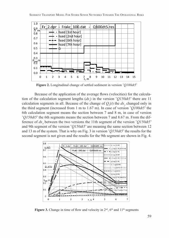
The longitudinal distribution of the settled sediment in the version ’Q100dt5’ at different moments can be seen on the Fig. 2. We drew also the diameters on the figure in order to see the ratios (now the calculated parameters are only for the 2nd-4th conduit sections, as done also later). The figure shows that the biggest settlement (hsed ≈ 22 cm) is in the first segment of the third conduit section (the first part of the pipe is filled almost half!). Between 6th and 7th hours, there is only a small difference, which is predictable from the Qi(t) curves.

The change in time of the flow (e.g. Q_6.seg[Q100]), the cross sectional average velocity (v_6.seg[Q100] [D=0,55]) and the depth of the settled sediment (h_6.seg[Q100]) in the 2nd, 6th and 11th calculation segments are given on the Fig. 3 and 4.

59


Figure 2. Longitudinal change of settled sediment in version ’Q100dt5’

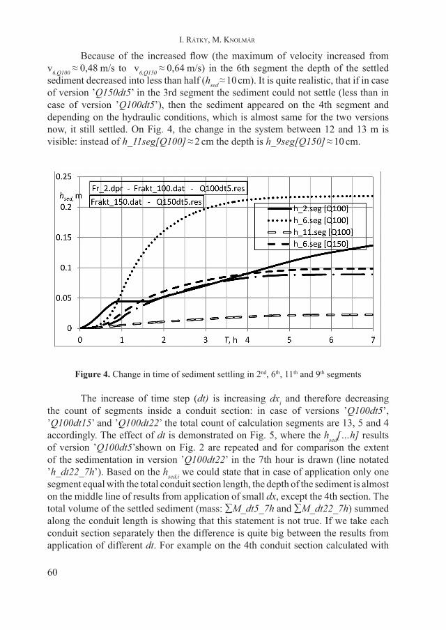
Because of the application of the average flows (velocities) for the calcula-tion of the calculation segment lengths (dxi) in the version ’Q150dt5’ there are 11 calculation segments in all. Because of the change of Q3(t) the dx3 changed only in the third segment (increased from 1 m to 1.67 m). In case of version ’Q100dt5’ the 6th calculation segment means the section between 7 and 8 m, in case of version ’Q150dt5’ the 6th segments means the section between 7 and 8.67 m. From the dif-ference of dx3 between the two versions the 11th segment of the version ’Q150dt5’ and 9th segment of the version ’Q150dt5’ are meaning the same section between 12 and 13 m of the system. That is why on Fig. 3 in version ’Q150dt5’ the results for the second segment is not given and the results for the 9th segment are shown in Fig. 4.

Figure 3. Change in time of flow and velocity in 2nd, 6th and 11th segments

60


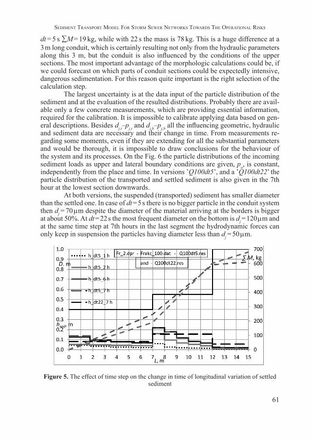
Because of the increased flow (the maximum of velocity increased from v6,Q100 ≈ 0,48 m/s to v6,Q150 ≈ 0,64 m/s) in the 6th segment the depth of the settled sediment decreased into less than half (hsed ≈ 10 cm). It is quite realistic, that if in case of version ’Q150dt5’ in the 3rd segment the sediment could not settle (less than in case of version ’Q100dt5’), then the sediment appeared on the 4th segment and depending on the hydraulic conditions, which is almost same for the two versions now, it still settled. On Fig. 4, the change in the system between 12 and 13 m is visible: instead of h_11seg[Q100] ≈ 2 cm the depth is h_9seg[Q150] ≈ 10 cm.

Figure 4. Change in time of sediment settling in 2nd, 6th, 11th and 9th segments

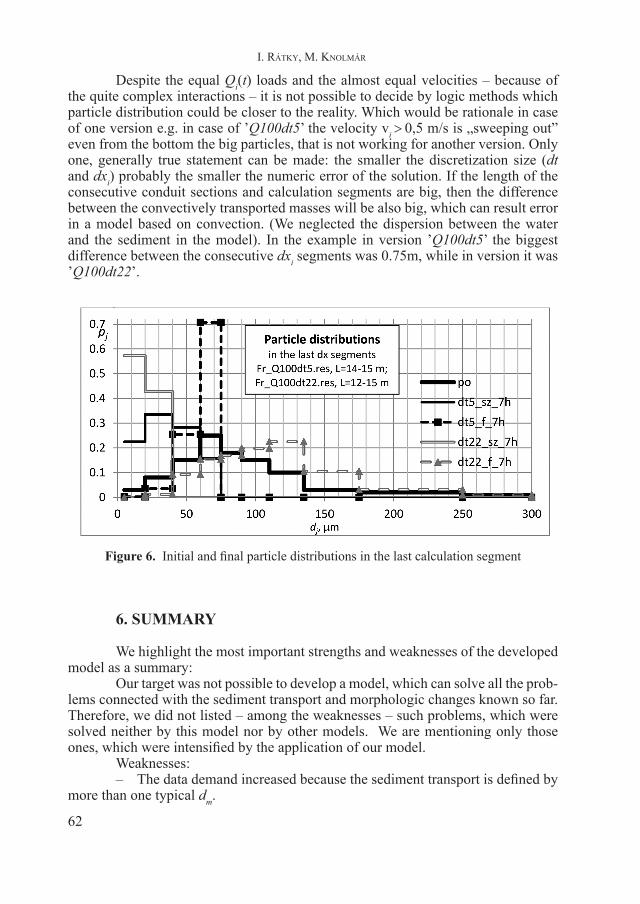
The increase of time step (dt) is increasing dxi and therefore decreasing the count of segments inside a conduit section: in case of versions ’Q100dt5’, ’Q100dt15’ and ’Q100dt22’ the total count of calculation segments are 13, 5 and 4 accordingly. The effect of dt is demonstrated on Fig. 5, where the hsed[…h] results of version ’Q100dt5’shown on Fig. 2 are repeated and for comparison the extent of the sedimentation in version ’Q100dt22’ in the 7th hour is drawn (line notated ’h_dt22_7h’). Based on the hsed,i we could state that in case of application only one segment equal with the total conduit section length, the depth of the sediment is almost on the middle line of results from application of small dx, except the 4th section. The total volume of the settled sediment (mass: ∑M_dt5_7h and ∑M_dt22_7h) summed along the conduit length is showing that this statement is not true. If we take each conduit section separately then the difference is quite big between the results from application of different dt. For example on the 4th conduit section calculated with

61


dt = 5 s ∑M = 19 kg, while with 22 s the mass is 78 kg. This is a huge difference at a 3 m long conduit, which is certainly resulting not only from the hydraulic parameters along this 3 m, but the conduit is also influenced by the conditions of the upper sections. The most important advantage of the morphologic calculations could be, if we could forecast on which parts of conduit sections could be expectedly intensive, dangerous sedimentation. For this reason quite important is the right selection of the calculation step.

The largest uncertainty is at the data input of the particle distribution of the sediment and at the evaluation of the resulted distributions. Probably there are avail-able only a few concrete measurements, which are providing essential information, required for the calibration. It is impossible to calibrate applying data based on gen-eral descriptions. Besides dj,t–pj,t and dj,b–pj,b all the influencing geometric, hydraulic and sediment data are necessary and their change in time. From measurements re-garding some moments, even if they are extending for all the substantial parameters and would be thorough, it is impossible to draw conclusions for the behaviour of the system and its processes. On the Fig. 6 the particle distributions of the incoming sediment loads as upper and lateral boundary conditions are given, po, is constant, independently from the place and time. In versions ’Q100dt5’, and a ’Q100dt22’ the particle distribution of the transported and settled sediment is also given in the 7th hour at the lowest section downwards.

At both versions, the suspended (transported) sediment has smaller diameter than the settled one. In case of dt = 5 s there is no bigger particle in the conduit system then dj = 70 µm despite the diameter of the material arriving at the borders is bigger at about 50%. At dt = 22 s the most frequent diameter on the bottom is dj = 120 µm and at the same time step at 7th hours in the last segment the hydrodynamic forces can only keep in suspension the particles having diameter less than dj = 50 µm.

Figure 5. The effect of time step on the change in time of longitudinal variation of settled sediment

62


Despite the equal Qi(t) loads and the almost equal velocities – because of the quite complex interactions – it is not possible to decide by logic methods which particle distribution could be closer to the reality. Which would be rationale in case of one version e.g. in case of ’Q100dt5’ the velocity vi > 0,5 m/s is „sweeping out” even from the bottom the big particles, that is not working for another version. Only one, generally true statement can be made: the smaller the discretization size (dt and dxi) probably the smaller the numeric error of the solution. If the length of the consecutive conduit sections and calculation segments are big, then the difference between the convectively transported masses will be also big, which can result error in a model based on convection. (We neglected the dispersion between the water and the sediment in the model). In the example in version ’Q100dt5’ the biggest difference between the consecutive dxi segments was 0.75m, while in version it was ’Q100dt22’.

Figure 6. Initial and final particle distributions in the last calculation segment

6. SUMMARy

We highlight the most important strengths and weaknesses of the developed model as a summary:

Our target was not possible to develop a model, which can solve all the prob-lems connected with the sediment transport and morphologic changes known so far. Therefore, we did not listed – among the weaknesses – such problems, which were solved neither by this model nor by other models. We are mentioning only those ones, which were intensified by the application of our model.

Weaknesses:– The data demand increased because the sediment transport is defined by

more than one typical dm.

63


– The calculation became more complicated.– The calibration became also more complicated and it needs more data. – We assumed each fraction to move separately, settling and mixing up

to process independently, without interactions to each other. Shading and cohesion effects are not including in the model. We mentioned them here as weakness points because a model applying and calibrating only for one dm can approximatively cal-culate with these effects.

Strengths:– The mixed particle structure i.e. particle diameter distribution (dj,t–p,j,t

and dj,f–pj,b) existing in the real sediment is included in the calculation of the sedi-ment transport (settling and mixing up).

– In a real conduit under transient and not permanent conditions, both set-tling and mixing-up processes are existing at the same time. Regarding these pro-cesses the model is calculating the morphologic change in a conduit section based on time step dt.

The most published models are assuming through a critical state (τcr or vcr) at the same time ether settling or mixing up state. And if this state is determined based on a typical dm parameter, then e.g. in case of a calculated settling state it is also assumed that even the smallest diameter of the mixed particle distribution is also settling, which is obviously not corresponding to the real situation.

The frame of this study did not allow executing a detailed sensitivity analysis for the data and the assumed parameters. The sensitivity analysis is worth performing before the build of the morphologic model into the hydraulic software system (SWMM or EPANET).

We should repeat because of its importance: the proper calibration of the model would be necessary; the quality of the calibration is significantly determined by the possibilities of the local measurements, the accuracy of the observations. Based on the available information, we tried to consider them during the model construction. The elaboration of all the small details is a future task.

REFERENCES

1. Danish Hydraulic Institute (DHI) (2008), MOUSE Pollution Transport, Reference Manual.

2. Danish Hydraulic Institute (DHI) (2009), Mike Urban Model Manager, User Guide.3. Delft3D-Flow (2011): User Manual, Simulation of multi-dimensional hydrodynam-

ic flows and transport phenomena, including sediments Version 3.15.4. Fan, C.Y.-Field, R.-Lai,F. (2003), Sewer-Sediment Control: Overview of an EPA

Wet-Weather Flow Research Program, U.S. Environmental Protection Agency. 5. Fan, C.Y. (2004): Sewer Sediment and Control, A Management Practices Reference

Guide, EPA/600/R-04/0596. Knolmár, M. (2011), Számítógéppel segített csatornatervezés (Computer Aided

sewer design) c. doktori (PhD) értekezés. BMGE Vízi Közmű és Környezetmérnöki Tanszék, Budapest.

64


7. Mannina, G.-Schellart, A.N.A.-Tait, S.-Viviani, G. (2012), Uncertainty in sew-er sediment deposit modelling: Detailed vs simplified modelling approaches, Physics and Chemistry of the Earth, Parts A/B/C 42-44:11-20.

8. MI-10-291/3-85 (1985), Műszaki hidraulika. Csővezetékek és csőhálózatok vízszállító képessége, Műszaki Irányelvek, OVH.

9. Rátky, I.-Rátky, É. (2013), Görgetett hordalék térfogatáram felső-dunai mérések alapján. MHT XXXI. Országos Vándorgyűlés Gödöllő 2013. július.

10. Roesner, L.A.-Aldrich, J.A.-Dickinson, R.E. (1992), Storm-Water Management Model User’s Manual Version 4: Extran Addendum, U.S. Environmental Protection Agency.

11. Rossman, L.A. (2010), Storm Water Management Model, User’s Manual, Version 5.0, U.S. Environmental Protection Agency.

12. Wallingford (2010), InfoWorks SD, Technical Review.13. van Rijn, L.C. (1984a), Sediment Transport, Part I: Bed Load Transport, Journal of

Hydraulic Engineering, Vol. 110, No. 10., pp. 1431-1456. 14. van Rijn L.C. (1984b), Sediment Transport, Part II: Suspended Load Transport,

Journal of Hydraulic Engineering, Vol. 110, No. 11. pp. 1613-1641.15. van Rijn L.C. (1985): Invited Lecture Euromech 192, Munich

SEDIMENT TRANSPORT MODEL FOR STORM SEWER...

Documents

Transcript of SEDIMENT TRANSPORT MODEL FOR STORM SEWER...